Volume 5 • Issue 6 • 1000204J Civil Environ EngISSN: 2165-784X JCEE, an open access journal

Jour

nal o

f Civi

l & Environmental Engineering

ISSN: 2165-784X

Journal of Civil & Environmental Engineering

Dang and Park, J Civil Environ Eng 2015, 5:6 DOI: 10.4172/2165-784X.1000204

Research Article Open Access

Numerical Simulation of Bed Level Variation in Open Channels Under Steady Flow ConditionsTruong AN Dang1* and Sang Deog Park2

1Sustainable Management of Natural Resources and Environment Research Group, Faculty of Environment and Labour Safety, Ton Duc Thang University, Ho Chi Minh City, Vietnam2Department of Civil Engineering, Prof. of Gangneung -Wonju National University/ South Korea

AbstractBed load transport is an important process in maintaining balance and stabilising channel geometry for restoring

the form and function of river ecosystems. The amount and spatial distribution of bed load sediment particles contribute significantly to riverbed level changes. The prediction of bed load sediment transport evolution is an important aspect of catchment planning. This work can be effectively supported through numerical simulation by detailed analyses of flow components and sediment transport inside watersheds. The purpose of this research is to develop a two-dimensional depth-averaged numerical model for flow and sediment transport using eight bed load transport equations to predict the time variation of bed deformation in steep slope, torrents and mountain river areas. The two-dimensional depth-averaged shallow water equations, along with the sediment continuity equation, are solved by using the Marker and Cell explicit scheme. Applying the eight bed load transport formulas to both ADM and MLSHM experimental flumes. After we will choice to the most appropriate formula to simulate the bed load transport rate and bed elevation change in the Yang yang mountains river in South Korea. The differences found between the measured experimental data and the numerical simulation for both flow and the time variations of bed deformation showed that the numerical model used in this research is useful for the analysis and prediction of riverbed level variations.

*Corresponding author: Truong An Dang, Sustainable Management of Natural Resources and Environment Research Group, Faculty of Environment and Labour Safety, Ton Duc Thang University, Ho Chi Minh City, Vietnam, Tel: (84-8) 37755055; E-mail: dangtruongan@tdt.edu.vn

Received November 14, 2015; Accepted December 02, 2015; Published December 12, 2015

Citation: Dang TAN, Park SD (2015) Numerical Simulation of Bed Level Variation in Open Channels Under Steady Flow Conditions. J Civil Environ Eng 5: 204. doi:10.4172/2165-784X.1000204

Copyright: © 2015 Dang TAN, et al. This is an open-access article distributed under the terms of the Creative Commons Attribution License, which permits unrestricted use, distribution, and reproduction in any medium, provided the original author and source are credited.

Keywords: Bed load transport; Bed level variation; Depth-averagedflow

IntroductionBed load transport is the physical process of shaping riverbeds and

affects both the form and function of many hydraulic structures in river ecosystems. Estimating the bed load transport rate is very important for realistic computations of variations in the riverbed topography. However, measuring the bed load transport rate is extremely difficult and very expensive [1-5]. Therefore, a process-based sediment dynamic modelling approach provides a wide range of options for evaluating the suitability of bed load transport equations in various conditions [6-10]. Thus far, most of the bed load transport equations have been conducted based only on limited laboratory scale experiments for the specific conditions in which they were developed or field conditions [11-20]. For this reason, some limitations to the universal application still exist. Therefore, experimental applications of existing bed load equations and their adaptability to different conditions can contribute valuable understanding for determining their optimal uses in specific cases and for different applications such as the accurate simulation of the bed load transport rate in rivers [21-29]. Gomez and Church [10] and Yang and Huang [29] investigated different bed load equations using measured data. They concluded that none of the equations could be universally accepted but also indicated that calibration would increase the predictive capability of each respective formula [16,18,24,27]. The aim of this study is to find a bed load transport formula that is suitable for bed load transport rate computation in steep slope areas, torrents and mountain river areas. This study uses different bed load transport formulas to estimate the rate of bed load sediment transport in open channels, to simulate riverbed level variations in a wide range of practical shallow open channel situations and to identify the optimum bed load transport formula to improve the accuracy and applicability of the calculation. This paper describes different bed load equations and their various parameters through their application to the experimental data. The relative performances of riverbed level simulations using different bed load equations are also presented in this paper [16-18,24]. In predicting the evolution process of riverbed elevation variations, numerical models have become popular because they can more

accurately simulate the hydrodynamic processes in rivers and are also less costly than other methods. Flexibility in designing for different plans, the ability to simulate river bed variations under large scale and long-term conditions, and providing a large quantity of useful information are a few of the reasons that numerical modelling is good choice for research. Currently, numerical modelling is widely used for all types of natural river flow and sediment transport problems [6,8,10,28,29] modelling is widely used for all types of natural river flow and sediment transport problems [6,8,10,28,29]. With advances in information technology, computational power is continuously increasing, so more sophisticated models are being developed in one-dimension (1D) and two-dimension (2D) problems and can even be extended to three dimensions (3D). 1D numerical modelling is the simplest mode of flow and sediment transport modelling because it involves equations only in one direction. It is also easy to simulate and calibrate quickly on computers. Many 1D models for simulating bed load sediment transport processes have been developed recently, such as the Mobed model by Krishnappan; Ialluvial model by Karim and Kennedy, Charima model by Holly; and 3ST1D model by Papanicolaou. Most of the 1D models that are presented here can predict water surface elevation and bed-elevation variations. However, 1D modelling cannot be implemented in cases where the longitudinal or vertical distributions of flow and suspended materials are also important. In many practical application problems, the river flows are very complex, and the assumptions of 1D flow may not be valid. Hydraulic engineers often

Volume 5 • Issue 6 • 1000204J Civil Environ EngISSN: 2165-784X JCEE, an open access journal

Citation: Dang TAN, Park SD (2015) Numerical Simulation of Bed Level Variation in Open Channels Under Steady Flow Conditions. J Civil Environ Eng 5: 204. doi:10.4172/2165-784X.1000204

Page 2 of 8

select 2D depth-averaged models in practice because of their efficiency and reasonable accuracy. A number of 2D numerical models have been developed for computing flow velocity and bed deformation in alluvial channels. Most of these models were developed to solve a specific type of sediment problem. The 2D models most can be vertically integrated and widely employed in engineering practice, such as the Seratra-2D model by Onishi and Wise; Sutrench-2D model by van Rijn and Tan; TABS-2 model by Thomas and McAnally; Mobed2 model by Spasojevic and Holly; ADCIRC model by Luettich; MIKE 21 model by Danish Hydraulic Institute; Unibest-TC model by Bosboom; FAST2D model by Minh Duc; FLUVIAL 12 model by Chang; Delft 2D model by Walstra; and the CCHE2D model by Jia and Wang. Application of the 2D models is more complicated than the 1D model, but is still simpler than the 3D models. 2D models are more popular models than other 3D models, but they are still able to provide sufficient quantities of information for project requirements and optimising resources. 3D models provide more information because they include the space of all (x, y, z) directions. They are usually applied in conditions where the flow is stratified turbulent flow, such as the Ecomsed model by Blumberg and Mellor; RMA10 model by King; EFDC3D model by Hamrick; CH3D-SED model by Spasojevic and Holly; MIKE3 model by the Danish Hydraulic Institute; FAST3D model by Landsberg; Delft 3D model by Delft Hydraulics; and the Telemac-3D model by Hervouet and Bates. However, they are very complicated and consume many resources in implementation. 3D models should be applied if very detailed distributions of desired quantity need to be simulated and flow characteristics are important in all directions. Each model (1D, 2D or 3D) is only applied for specific purposes; for example, the 1D TUFLOW model was developed for determining flow patterns in coastal waters, estuaries, rivers and floodplains; the 2D MIKE 21 Flow Model was developed to simulate hydraulic and environmental phenomena in lakes, estuaries, bays, coastal areas and seas; and the Delft-3D model was developed for simulations of flows, sediment transports, waves, water quality, morphological developments and ecology. Therefore, a numerical model cannot be appropriately applied to calculate all of these cases [6,7,11,13,17,20,26,28]. The purpose of this research is to develop a 2D depth-averaged numerical model to simulate flow velocity and sediment transport in steep slope river areas, torrents and mountain river areas. We used the Cartesian coordinate system to apply in this model. The numerical solution is implemented on a staggered grid, and the time step is set as an expression that only depends on the grid spacing and the velocity components in the x-and y-directions. This procedure allows the coupling of variables and consequently improves the stability constraints. A commonly used staggered grid will be used as a prototype for investigating numerical solutions. Because it is apparent that two super-imposed grids are involved, they will be identified as primary and secondary grids. For the numerical solution procedure, the explicit Marker and Cell method is used to solve the 2D shallow water system of equations and the sediment continuity equation. First order approximation was used for the temporal derivative, and second order central difference approximations were used for space discretisation. The time step is limited by the Courant Friedrichs Lewy (CFL) stability condition. The approach is used with an iterative method in this research. The method is implemented by a computer source code and is written in the structured Fortran 90 programming language. Finally, the model is compared to the experimental data of the aggradation depths measured by Soni and the Large Scale Hydraulic Models (LSHM) of the University of Calabria, Italy to verify its applicability [17,19,21,22,28].

Numerical MethodGoverning equations

Most open channel flow models are relatively shallow water problems, so the effect of the vertical motion of the flow velocity is usually ignored. By assuming hydrostatic pressure distribution and neglecting wind shear and Coriolis acceleration, the depth-averaged 2D Navier-Stokes equations system are expressed in Cartesian coordinates in the following form [1,3,7,13,17,20]:

x yh (q ) (q ) 0t x y

∂ ∂ ∂+ + =

∂ ∂ ∂ (1)

( )2

x yxx ox fx

q qq h(q ) ( ) ( ) gh gh S -St x h y h x∂ ∂ ∂ ∂

+ + = − +∂ ∂ ∂ ∂

(2)

( )2

x y yy oy fy

q q q h(q ) ( ) ( ) gh gh S -St x h y h y∂ ∂ ∂ ∂

+ + = − +∂ ∂ ∂ ∂

(3)

where t is the time; h is the water depth; qx=uh and qy=vh are the discharge intensities on a unit area in the x and y directions, respectively; u and v are the averaged components of the velocity components in the x-and y-directions, respectively; g is the acceleration of gravity; n is Manning’s roughness coefficient; Sox and Soy are the bed slopes of the channel in the x and y directions, respectively; and Sfx and Sfy are the friction slopes in the x and y directions, respectively, which can be computed as follows:

2 2 2x x y

fx 43

n q q qS

h

+= (4)

2 2 2y x y

fy 43

n q q qS

h

+= (5)

ox oyz zS ; Sx y∂ ∂

= − = −∂ ∂ (6)

The above equations (1) through (3) were used to apply to the numerical scheme on a staggered grid, where an explicit difference formulation first-order approximation was used for the temporal derivative (∆t) and second-order central difference approximations were used for space discretisation (∆x, ∆y). The magnitude of the time step is almost the same explicit difference scheme as the Mac Cormack, Lax-Wendroff and Marker and Cell scheme is governed by the CFL stability condition. In this study, the time step is calculated based on the grid spacing (∆x, ∆y) and the velocity components in the x-and y-directions [3-5,19-22,28,30,31].

( )( )2 2

2 2 2 2

x ytu v gh x y

∆ ∆∆ = α

+ + ∆ +∆ (7)

where ∆t is the time increment (sec); ∆x, ∆y are the grid spacings in x, y directions, respectively;

u, v are the averaged components of the flow velocity in the x, y directions, respectively;

h is the water depth; α is the coefficient (α ≤1)

g is the acceleration of the gravity

Sediment transport equations

By considering only the bed load transport and neglecting particle sorting in a uniform sediment, the two-dimensional sediment continuity equation may be written as [6,14-16,28].

byb bxqZ q1 0

t 1 p x y∂ ∂ ∂

+ + = ∂ − ∂ ∂ (8)

Volume 5 • Issue 6 • 1000204J Civil Environ EngISSN: 2165-784X JCEE, an open access journal

Citation: Dang TAN, Park SD (2015) Numerical Simulation of Bed Level Variation in Open Channels Under Steady Flow Conditions. J Civil Environ Eng 5: 204. doi:10.4172/2165-784X.1000204

Page 3 of 8

Where Zb is the local bed elevation; p is the porosity of the bed

material; ∂Zb is the change in the local bed level during the time interval ∂t; and qbx, qby are the x, y components of the bed load transport per unit width.

The dominant physical variables of the bed load transport processes are usually water discharge, average flow velocity, energy slope, and shear stress at the channel bottom [2,6,8,15,25,30]. Bed load transport equations have generally been developed based on the solutions of shallow water equations, and then the equations were calibrated to differing degrees to suit site-specific conditions. In this study, eight widely used bed load transport equations (Table 1), were reviewed and incorporated into the process based sediment dynamic model to estimate bed load transport rates and river bed level variations [2,6,8,10,11,15,25,28,29]. In the above formulas, qb is the bed load transport; q is water discharge; S is the bottom slope; D50 is the particle diameter; τ is the bed shear stress; τc is the critical shear stress; γs, γ are the specific weights of sediment and water, respectively; τc

*

is the dimensionless critical stress; and g is gravitational acceleration. In the Meyer-Peter equation, the constants 17 and 0.4 are valid only for sand with a specific gravity of 2.65. The Meyer-Peter formula can only be applied to coarse materials with particle sizes greater than 3 mm. For mixtures of non-uniform materials, D50 should be replaced by D35 [2,14,24,25,29,30]. In the Engelund and Fredsoe equation, τc

*=0.05; τ* is the dimensionless Shields stress. In the Madsen equation, FM =9.5 for saltating sand grains in water. In the Bagnold’s formula, τc

*is the dimensionless critical stress for incipient motion (=0.05) for D50 of a uniform material ranging in size from 0.3 mm to 7.0 mm [2,6,8,11,14,15,24,25,29,30].

Discretisation of governing equations

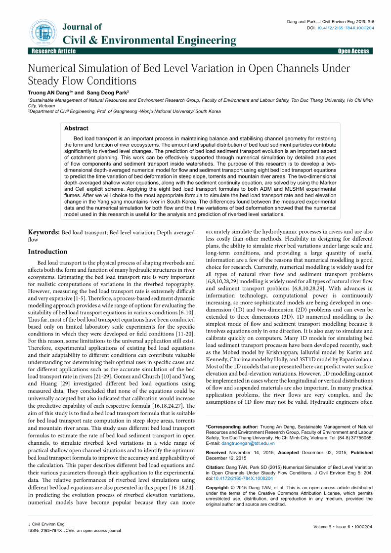
The governing equations are solved on a staggered grid. In the research domain, the water depth (h) is defined on the primary grid centre (i, j), whereas the velocity components (u, v) are defined on the cell faces of the secondary grid (i+1/2, j+1/2) (Figure 1). More precisely, the u-component of the velocity is assigned to the one-half grid line in the x-direction. The v-component of the velocity is defined in a similar fashion on the one-half grid line in the y-direction [11,13,14,21].

Equation (1) is applied at grid point (i, j), yielding the following finite difference equation:

( ) ( ) ( ) ( )1 1 1 12 2 2 2

T 1 T 1T 1 T 1T 1 Ti,j i,j x x y yi ,j i ,j i,j i,j

t tH H q q q qx y

+ ++ +++ − + −

∆ ∆ = − − − − ∆ ∆ (9)

The x-momentum equation is applied on the secondary grid at grid point (i+1/2, j):

( ) ( ) ( ) ( )

73

2 2 T TT 1 T T T T T1 1 1 11 1 1 I 1,J I,J I 1,J I,J I ,J I ,JI ,J I ,J I ,J 2 2 2 21 12 2 2 I ,J I ,J

2 2

T T 2 T T 21 I 1,J I,J 1 1 1I ,J I ,J I ,J I ,J2 2 2 2

t t 1 t 1P P H H H P P g PQ PQx x H y H

tg H Z Z tgn H P (P )x

−

++ + + + + −+ + +

+ +

++ + + +

∆ ∆ ∆ = − − + − − − ∆ ∆ ∆

∆ − − −∆ ∆

T 2 T1I,J2

(Q )+

+

(10)

Finally, we obtain the finite difference equation of the x-momentum equation:

2 2

T 1 T 2 T 2 T T T T T1 1 I 1,J I,J 3 1 1 1I ,J I ,J I ,J I ,J I ,J I ,J

12 2 2 2 2 2I ,J2

T T T T1 1 1 1I ,J I ,J 1 I,J I 1,J

1 2 2 2 2I ,J2

g t 1 t 1P P (H ) (H ) P P P P2 x 4 x H

1 t 1 P P Q Q4 y H

++

+ + + + + −+

+ + + + + ++

∆ ∆ = − − + + − + ∆ ∆

∆− + + ∆

73

T T T T1 1 1 1I ,J I ,J-1 I,J- I 1,J-

1 2 2 2 2I ,J2

T T 2 T T 2 T 2 T1 I 1,J I,J 1 1 1 1I ,J I ,J I ,J I ,J I,J2 2 2 2 2

1 t 1 P P Q Q4 y H

tg H Z Z tgn H P (P ) (Q )x

−

+ + ++

++ + + + +

∆+ + + ∆

∆ − − −∆ + ∆

(11)

Similarly, the y-component of the momentum equation is applied at grid point (i, j+1/2), yielding the following finite difference equation:

( ) ( ) ( ) ( )2 2T TT 1 T T T1 1 1 11 1 I,J 1 I,JT TI ,J I- ,JI,J I,J 2 2 2 21 12 2 I,J I,J

2 2

T T T T T T1 I,J 1 I,J 1 I,J 1 I,JI,J I,J2 2

73

2 T T 21 1I,J I,J I2 2

t 1 t 1Q Q PQ PQ Q Qx h y H

t tg H H H g H Z Zy y

gn t H Q (P )

+++ + ++ +

+ +

+ ++ +

−

+ + +

∆ ∆ = − − − − ∆ ∆

∆ ∆ − − − − ∆ ∆

− ∆

T 2 T1 1,J I,J2 2

(Q )+

+

(12)

Finally, we obtain the finite difference equation of the y-momentum equation:

T 1 T T T T T1 1 1 1 1 1I,J I,J I ,J I ,J 1 I,J I 1,J

12 2 2 2 2 2I,J2

T T T T1 1 1 1I- ,J I ,J 1 I,J I 1,J

1 2 2 2 2I,J2

T3T I,J I

1 2I,J2

1 t 1Q Q P P Q Q4 x H

1 t 1 P P Q Q4 x H

1 t 1 Q Q4 y H

+

+ + + + + + + ++

− + + − ++

++

∆= − + + ∆

∆+ + + ∆

∆− +

∆

2 2

T T T T T T1 1 1 1 I,J 1 I,J,J I,J I,J I,J2 2 2 2

73

T T T 2 T T 2 T 2 T1 I,J 1 I,J 1 1 1 1I,J I,J I,J I ,J I,J2 2 2 2 2

tQ Q g H H Hy

tg H Z Z gn t H Q (P ) (Q )y

++ + − +

−

++ + + + +

∆ − + − − ∆

∆ − − − ∆ + ∆

(13)

Observe that the discharge components are specified at the (n+1) time step in equation (7). However, this poses no difficulty because

Figure 1: Staggered grid with boundary cells.

Author(s) Bed Load Formulas

Duboys ( )b c34

50

0.173qD

= τ τ− τ

Shields ( )b s c

s 50

q -10

qS Dγ τ τ=

γ γ − γ

Schoklitsch ( )3

23

27

6

50b c c

0.6Dq 2500S q q qS

= − =

Bagnold ( )[ ]*c

**c

*b ττττ17q −−=

Engelund and Fredsoe ( ) ( ) ( )1 1

2 2* * * *b c cq 18.74 0.7 = τ − τ τ − τ

Madsen ( )*

c*2

1*c

21*

Mb τττ0.7τFq −

−=

Nielsen ( )*c

*21*

b τττ12q −=

Cheng (2002)3* 2

b 3* 2

0.05q 13 exp -

= τ τ

Table 1: List of selected bed load equations used in this research.

Volume 5 • Issue 6 • 1000204J Civil Environ EngISSN: 2165-784X JCEE, an open access journal

Citation: Dang TAN, Park SD (2015) Numerical Simulation of Bed Level Variation in Open Channels Under Steady Flow Conditions. J Civil Environ Eng 5: 204. doi:10.4172/2165-784X.1000204

Page 4 of 8

the momentum equations (10) and (12) in the x and y directions are solved first to provide PI+1/2,J and QI, J+1/2, the values of the discharge components at the (n+1) time step. The water depth at the (n+1) time step in equation (7) is then solved. Equation (7) is solved iteratively to determine the value of Hi, j at time step (n+1) over the entire domain. Subsequently, equations (10) and (12) are used to compute the velocity components or discharge components at time step (n+1) over the entire domain [12,17,19-21,28] .

Boundary conditions

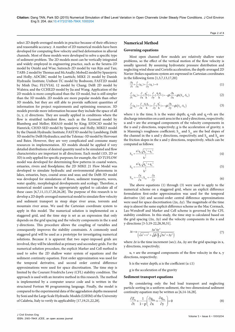
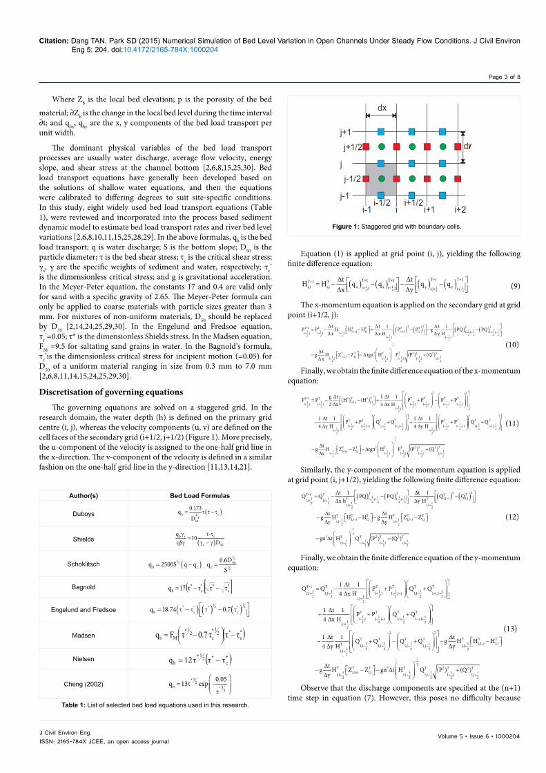
The physical boundaries of a specified domain upon which the boundary conditions are imposed include the following types: upstream, downstream, and solid boundaries. Two boundary conditions are usually required at an upstream boundary. The y-component of the velocity may be set at zero or may be determined by setting the velocity gradient dv/dx to zero [9,12,14,17,20]. If one uses a first-order approximation, v1,j = v2,j, an approximation of a higher order can be used, such as the following formula: v1,j = 2v2,j – v3,j. In this study, the water depth (h) and the x-component of the flow velocity were provided in the form of a time series hydrograph. The v-component of the flow velocity was set to zero. At the downstream boundary, the values of the velocity components and the water depth are typically not known. Therefore, for most applications, Neumann-type boundary conditions are imposed. A zero value for the velocity gradient may be appropriate for the downstream boundary. At a solid boundary, there is no relative motion between the solid boundary and the fluid boundary. However, the Marker and Cell method used in this study requires some values for the velocity components outside the calculation domain. These values are essentially obtained by extrapolation of the interior points or, equivalently, by approximation of the derivatives at the solid boundary. An assumed solid boundary is aligned along j=1/2, and an inflow boundary is aligned along i=1/2 (Figure 2). The no-slip condition is imposed. Therefore, v1,1/2 = v2,1/2=…= 0. Similarly, u3/2,1/2 = 0, from which u3/2, 1/2 is approximated by u3/2,1/2=1/2(u3/2,0 + u3/2,1) = 0 or u3/2,0 = -u3/2,1. The values of the velocity components at the solid boundary are set to zero [12,20-22]. The steps in the process for solving the flow and bed load sediment equations are listed below and are illustrated in Figure 3.

Step 1: Initialize all the variables. This step usually corresponds to a time level of T0. At this step the values of the water depth as well as flow field within computational domain and boundaries are specifically established. It is supposed that the velocity components and water depth are known at a given time T0, and that the boundary conditions for the velocity components and water depth are also given.

Step 2: The partial differential equations (21) (22), and (23) for the flow, and for the sediment continuity equation (24) are solved with

the finite difference code. The discretized equations are obtained for the shallow water and sediment continuity equations by the staggered numerical grid. An initial and boundary conditions used to solve the momentum equations (22), (23) and then the continuity equation (21) the values of u, v, and h at the new time level T+1 are determined at every interior node (I = 2,...,N). The values of the dependent variables u, v at the boundary nodes 1 and N+1 are determined by using the boundary conditions. The values of the dependent variables that are not specified through boundary conditions can be determined by extrapolation of the interior points or equivalently by approximation of the derivatives at the fictitious boundary points. We then obtain the corrected water depth and (u, v) velocity components at every interior node in the computational domain.

Step 3: The velocity components calculation at time step T=T0+ΔT until a converged solution is obtained. At this step, convergence criteria must be checked because the scheme used in this research is iterative scheme. Then, update the velocity components and water depth with their corresponding values.

Step 4: Use the water depth and velocity components to calculate dimensionless particle diameter; dimensionless Shields tress; dimensionless critical Shields tress; critical shear tress; boundary shear stress, etc. Where dimensionless particle diameter is calculated. The program provides the selection of the following empirical formulas for shear stress: USWES formula; Krey formula; Chang formula, and Sakai formula.

Step 5: Use the calculated parameters from Step 4 to take into one of the equations such as DuBoy; Cheng; Shield; Madsen; Engelund & Fredsoe; Nielsen; Bagnold; Schoklitsch to calculate the bed load transport rate. The program provides the selection of the following nine bed load formulas.

Step 6: Calculate the erosion and deposition by using the sediment continuity equation (4.15) to determine the bed level variation and update the new water depth if the channel bed is changed.

Step 7: Return to Step 2 and repeat the preceding calculation until the specified final time level. If a steady state solution is required, a specified convergence criterion must be satisfied.

Step 8: The last step in the calculation process involves store and

Figure 2: Illustration of specification of the boundary conditions on a staggered grid.

Figure 3: Flow chart for numerical simulation model.

Volume 5 • Issue 6 • 1000204J Civil Environ EngISSN: 2165-784X JCEE, an open access journal

Citation: Dang TAN, Park SD (2015) Numerical Simulation of Bed Level Variation in Open Channels Under Steady Flow Conditions. J Civil Environ Eng 5: 204. doi:10.4172/2165-784X.1000204

Page 5 of 8

update variables at each time step and moving to the next time step and repeat Step 2 to Step 7.

Application of model testing, verification and discussion

To investigate the applicability of the numerical model developed in this research, two sets of bed topography evolution measurements were used from the experimental flumes. The first set was obtained from the Aggradation Depths Measurements (ADM) (Figure 4), obtained by Soni (1981a) in a laboratory flume with a rectangular cross section. The second set was obtained at the Large Scale Hydraulic Model (LSHM) at the University of Calabria, Italy (Figure 5) [2,3,18]. The parameters for these tests are as follows: discharge Q; flume length and width L, B; water depth H; the porosity p; bed channel slope S; median particle diameter D50. Both experiments used sediment with a specific gravity of 2.65, and the other values are given in Table 2 [2,3,18]. In this research, the expression for calculating the mean absolute error (MAE) (the flow velocity form is presented in equation (14)) was selected to determine the error between the calculated results and the measured data so that the mean absolute percentage error between calculated results and measured data is minimised. The mean absolute percentage error is defined as follows:

Measured Value Calculated Value

Measured Value

U U100MAEN U

−= ∑ (14)

Where UMeasured Value is the measured velocity;

UCalculated Value is the calculated velocity; and

N is the total number of samples.

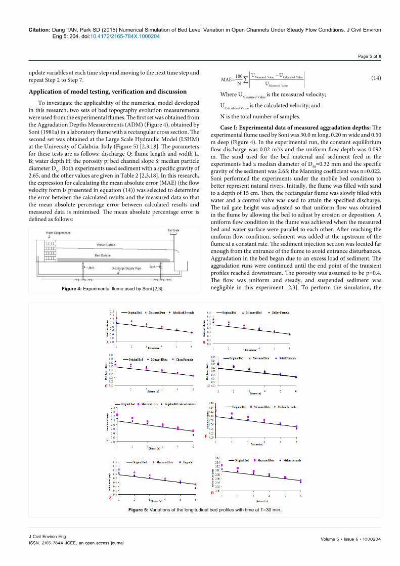
Case I: Experimental data of measured aggradation depths: The experimental flume used by Soni was 30.0 m long, 0.20 m wide and 0.50 m deep (Figure 4). In the experimental run, the constant equilibrium flow discharge was 0.02 m3/s and the uniform flow depth was 0.092 m. The sand used for the bed material and sediment feed in the experiments had a median diameter of D50=0.32 mm and the specific gravity of the sediment was 2.65; the Manning coefficient was n=0.022. Soni performed the experiments under the mobile bed condition to better represent natural rivers. Initially, the flume was filled with sand to a depth of 15 cm. Then, the rectangular flume was slowly filled with water and a control valve was used to attain the specified discharge. The tail gate height was adjusted so that uniform flow was obtained in the flume by allowing the bed to adjust by erosion or deposition. A uniform flow condition in the flume was achieved when the measured bed and water surface were parallel to each other. After reaching the uniform flow condition, sediment was added at the upstream of the flume at a constant rate. The sediment injection section was located far enough from the entrance of the flume to avoid entrance disturbances. Aggradation in the bed began due to an excess load of sediment. The aggradation runs were continued until the end point of the transient profiles reached downstream. The porosity was assumed to be p=0.4. The flow was uniform and steady, and suspended sediment was negligible in this experiment [2,3]. To perform the simulation, the

Figure 4: Experimental flume used by Soni [2,3].

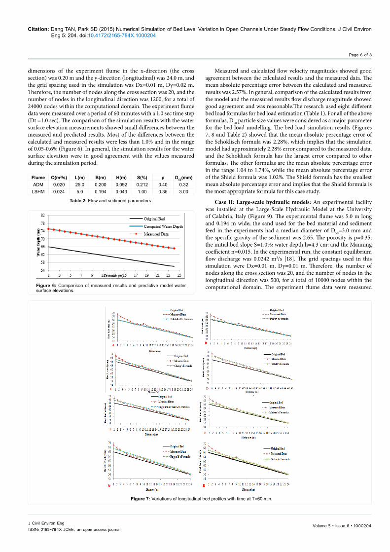
Figure 5: Variations of the longitudinal bed profiles with time at T=30 min.

Volume 5 • Issue 6 • 1000204J Civil Environ EngISSN: 2165-784X JCEE, an open access journal

Citation: Dang TAN, Park SD (2015) Numerical Simulation of Bed Level Variation in Open Channels Under Steady Flow Conditions. J Civil Environ Eng 5: 204. doi:10.4172/2165-784X.1000204

Page 6 of 8

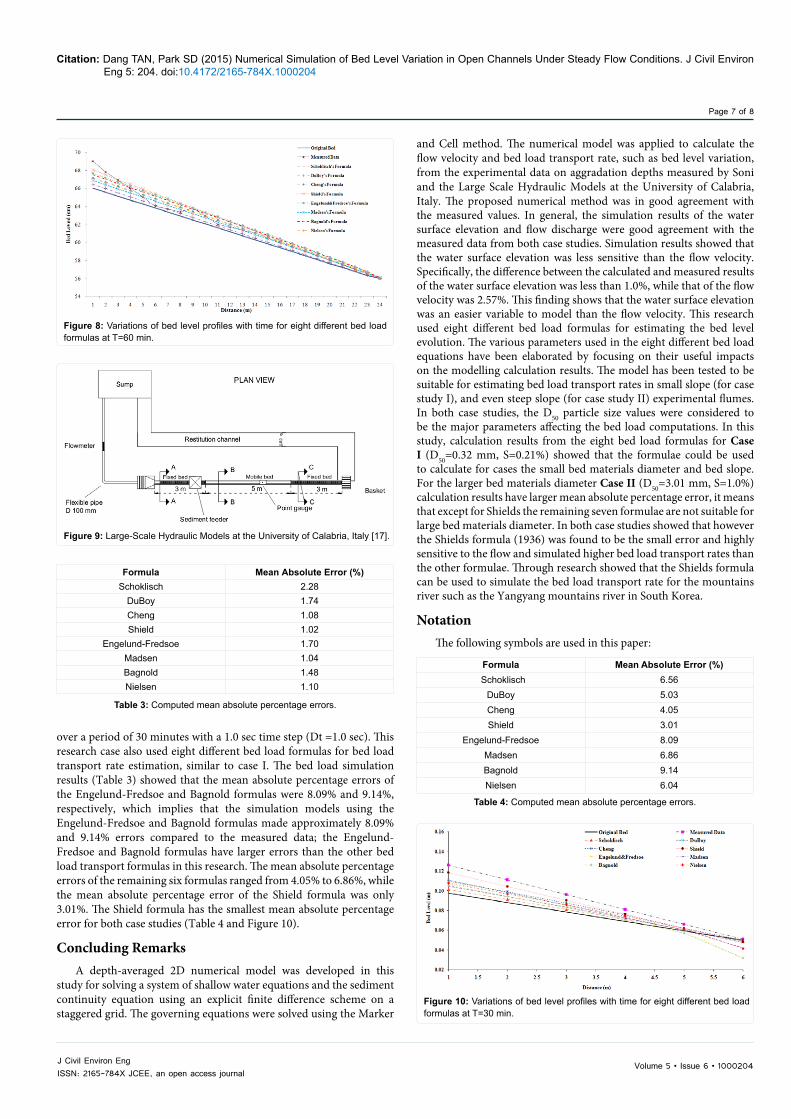
dimensions of the experiment flume in the x-direction (the cross section) was 0.20 m and the y-direction (longitudinal) was 24.0 m, and the grid spacing used in the simulation was Dx=0.01 m, Dy=0.02 m. Therefore, the number of nodes along the cross section was 20, and the number of nodes in the longitudinal direction was 1200, for a total of 24000 nodes within the computational domain. The experiment flume data were measured over a period of 60 minutes with a 1.0 sec time step (Dt =1.0 sec). The comparison of the simulation results with the water surface elevation measurements showed small differences between the measured and predicted results. Most of the differences between the calculated and measured results were less than 1.0% and in the range of 0.05-0.6% (Figure 6). In general, the simulation results for the water surface elevation were in good agreement with the values measured during the simulation period.

Figure 6: Comparison of measured results and predictive model water surface elevations.

Flume Q(m3/s) L(m) B(m) H(m) S(%) p D50(mm)ADM 0.020 25.0 0.200 0.092 0.212 0.40 0.32

LSHM 0.024 5.0 0.194 0.043 1.00 0.35 3.00

Table 2: Flow and sediment parameters.

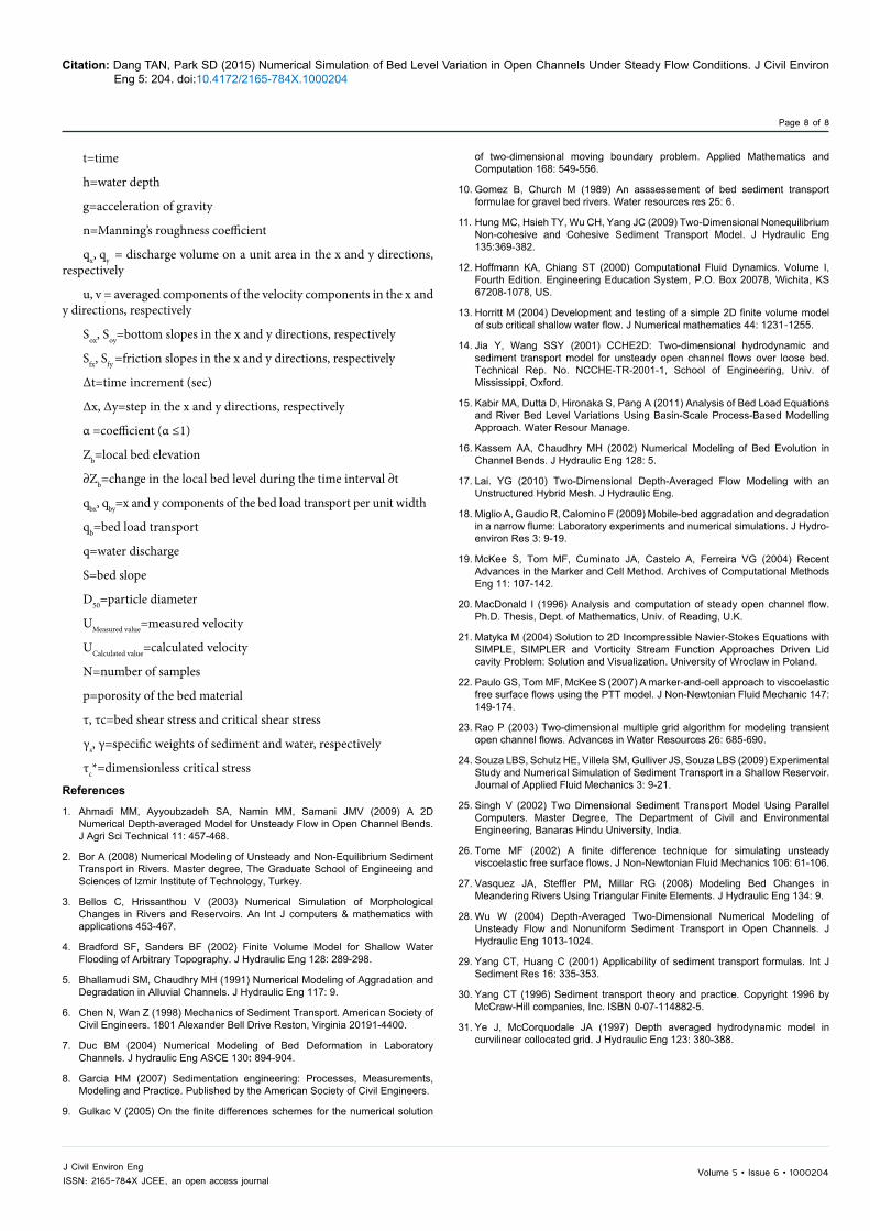
Measured and calculated flow velocity magnitudes showed good agreement between the calculated results and the measured data. The mean absolute percentage error between the calculated and measured results was 2.57%. In general, comparison of the calculated results from the model and the measured results flow discharge magnitude showed good agreement and was reasonable.The research used eight different bed load formulas for bed load estimation (Table 1). For all of the above formulas, D50 particle size values were considered as a major parameter for the bed load modelling. The bed load simulation results (Figures 7, 8 and Table 2) showed that the mean absolute percentage error of the Schoklisch formula was 2.28%, which implies that the simulation model had approximately 2.28% error compared to the measured data, and the Schoklisch formula has the largest error compared to other formulas. The other formulas are the mean absolute percentage error in the range 1.04 to 1.74%, while the mean absolute percentage error of the Shield formula was 1.02%. The Shield formula has the smallest mean absolute percentage error and implies that the Shield formula is the most appropriate formula for this case study.

Case II: Large-scale hydraulic models: An experimental facility was installed at the Large-Scale Hydraulic Model at the University of Calabria, Italy (Figure 9). The experimental flume was 5.0 m long and 0.194 m wide; the sand used for the bed material and sediment feed in the experiments had a median diameter of D50=3.0 mm and the specific gravity of the sediment was 2.65. The porosity is p=0.35; the initial bed slope S=1.0%; water depth h=4.3 cm; and the Manning coefficient n=0.015. In the experimental run, the constant equilibrium flow discharge was 0.0242 m3/s [18]. The grid spacings used in this simulation were Dx=0.01 m, Dy=0.01 m. Therefore, the number of nodes along the cross section was 20, and the number of nodes in the longitudinal direction was 500, for a total of 10000 nodes within the computational domain. The experiment flume data were measured

Figure 7: Variations of longitudinal bed profiles with time at T=60 min.

Volume 5 • Issue 6 • 1000204J Civil Environ EngISSN: 2165-784X JCEE, an open access journal

Citation: Dang TAN, Park SD (2015) Numerical Simulation of Bed Level Variation in Open Channels Under Steady Flow Conditions. J Civil Environ Eng 5: 204. doi:10.4172/2165-784X.1000204

Page 7 of 8

over a period of 30 minutes with a 1.0 sec time step (Dt =1.0 sec). This research case also used eight different bed load formulas for bed load transport rate estimation, similar to case I. The bed load simulation results (Table 3) showed that the mean absolute percentage errors of the Engelund-Fredsoe and Bagnold formulas were 8.09% and 9.14%, respectively, which implies that the simulation models using the Engelund-Fredsoe and Bagnold formulas made approximately 8.09% and 9.14% errors compared to the measured data; the Engelund-Fredsoe and Bagnold formulas have larger errors than the other bed load transport formulas in this research. The mean absolute percentage errors of the remaining six formulas ranged from 4.05% to 6.86%, while the mean absolute percentage error of the Shield formula was only 3.01%. The Shield formula has the smallest mean absolute percentage error for both case studies (Table 4 and Figure 10).

Concluding Remarks A depth-averaged 2D numerical model was developed in this

study for solving a system of shallow water equations and the sediment continuity equation using an explicit finite difference scheme on a staggered grid. The governing equations were solved using the Marker

and Cell method. The numerical model was applied to calculate the flow velocity and bed load transport rate, such as bed level variation, from the experimental data on aggradation depths measured by Soni and the Large Scale Hydraulic Models at the University of Calabria, Italy. The proposed numerical method was in good agreement with the measured values. In general, the simulation results of the water surface elevation and flow discharge were good agreement with the measured data from both case studies. Simulation results showed that the water surface elevation was less sensitive than the flow velocity. Specifically, the difference between the calculated and measured results of the water surface elevation was less than 1.0%, while that of the flow velocity was 2.57%. This finding shows that the water surface elevation was an easier variable to model than the flow velocity. This research used eight different bed load formulas for estimating the bed level evolution. The various parameters used in the eight different bed load equations have been elaborated by focusing on their useful impacts on the modelling calculation results. The model has been tested to be suitable for estimating bed load transport rates in small slope (for case study I), and even steep slope (for case study II) experimental flumes. In both case studies, the D50 particle size values were considered to be the major parameters affecting the bed load computations. In this study, calculation results from the eight bed load formulas for Case I (D50=0.32 mm, S=0.21%) showed that the formulae could be used to calculate for cases the small bed materials diameter and bed slope. For the larger bed materials diameter Case II (D50=3.01 mm, S=1.0%) calculation results have larger mean absolute percentage error, it means that except for Shields the remaining seven formulae are not suitable for large bed materials diameter. In both case studies showed that however the Shields formula (1936) was found to be the small error and highly sensitive to the flow and simulated higher bed load transport rates than the other formulae. Through research showed that the Shields formula can be used to simulate the bed load transport rate for the mountains river such as the Yangyang mountains river in South Korea.

NotationThe following symbols are used in this paper:

Figure 8: Variations of bed level profiles with time for eight different bed load formulas at T=60 min.

Figure 9: Large-Scale Hydraulic Models at the University of Calabria, Italy [17].

Figure 10: Variations of bed level profiles with time for eight different bed load formulas at T=30 min.

Formula Mean Absolute Error (%)Schoklisch 2.28

DuBoy 1.74Cheng 1.08Shield 1.02

Engelund-Fredsoe 1.70Madsen 1.04Bagnold 1.48Nielsen 1.10

Table 3: Computed mean absolute percentage errors.

Formula Mean Absolute Error (%)Schoklisch 6.56

DuBoy 5.03Cheng 4.05Shield 3.01

Engelund-Fredsoe 8.09Madsen 6.86Bagnold 9.14Nielsen 6.04

Table 4: Computed mean absolute percentage errors.

Volume 5 • Issue 6 • 1000204J Civil Environ EngISSN: 2165-784X JCEE, an open access journal

Citation: Dang TAN, Park SD (2015) Numerical Simulation of Bed Level Variation in Open Channels Under Steady Flow Conditions. J Civil Environ Eng 5: 204. doi:10.4172/2165-784X.1000204

Page 8 of 8

t=time

h=water depth

g=acceleration of gravity

n=Manning’s roughness coefficient

qx, qy = discharge volume on a unit area in the x and y directions, respectively

u, v = averaged components of the velocity components in the x and y directions, respectively

Sox, Soy=bottom slopes in the x and y directions, respectively

Sfx, Sfy =friction slopes in the x and y directions, respectively

∆t=time increment (sec)

∆x, ∆y=step in the x and y directions, respectively

α =coefficient (α ≤1)

Zb=local bed elevation

∂Zb=change in the local bed level during the time interval ∂t

qbx, qby=x and y components of the bed load transport per unit width

qb=bed load transport

q=water discharge

S=bed slope

D50=particle diameter

UMeasured value=measured velocity

UCalculated value=calculated velocity

N=number of samples

p=porosity of the bed material

τ, τc=bed shear stress and critical shear stress

γs, γ=specific weights of sediment and water, respectively

τc*=dimensionless critical stress

References

1. Ahmadi MM, Ayyoubzadeh SA, Namin MM, Samani JMV (2009) A 2D Numerical Depth-averaged Model for Unsteady Flow in Open Channel Bends. J Agri Sci Technical 11: 457-468.

2. Bor A (2008) Numerical Modeling of Unsteady and Non-Equilibrium Sediment Transport in Rivers. Master degree, The Graduate School of Engineeing and Sciences of Izmir Institute of Technology, Turkey.

3. Bellos C, Hrissanthou V (2003) Numerical Simulation of Morphological Changes in Rivers and Reservoirs. An Int J computers & mathematics withapplications 453-467.

4. Bradford SF, Sanders BF (2002) Finite Volume Model for Shallow Water Flooding of Arbitrary Topography. J Hydraulic Eng 128: 289-298.

5. Bhallamudi SM, Chaudhry MH (1991) Numerical Modeling of Aggradation and Degradation in Alluvial Channels. J Hydraulic Eng 117: 9.

6. Chen N, Wan Z (1998) Mechanics of Sediment Transport. American Society of Civil Engineers. 1801 Alexander Bell Drive Reston, Virginia 20191-4400.

7. Duc BM (2004) Numerical Modeling of Bed Deformation in Laboratory Channels. J hydraulic Eng ASCE 130: 894-904.

8. Garcia HM (2007) Sedimentation engineering: Processes, Measurements, Modeling and Practice. Published by the American Society of Civil Engineers.

9. Gulkac V (2005) On the finite differences schemes for the numerical solution

of two-dimensional moving boundary problem. Applied Mathematics and Computation 168: 549-556.

10. Gomez B, Church M (1989) An asssessement of bed sediment transport formulae for gravel bed rivers. Water resources res 25: 6.

11. Hung MC, Hsieh TY, Wu CH, Yang JC (2009) Two-Dimensional Nonequilibrium Non-cohesive and Cohesive Sediment Transport Model. J Hydraulic Eng 135:369-382.

12. Hoffmann KA, Chiang ST (2000) Computational Fluid Dynamics. Volume I, Fourth Edition. Engineering Education System, P.O. Box 20078, Wichita, KS 67208-1078, US.

13. Horritt M (2004) Development and testing of a simple 2D finite volume model of sub critical shallow water flow. J Numerical mathematics 44: 1231-1255.

14. Jia Y, Wang SSY (2001) CCHE2D: Two-dimensional hydrodynamic and sediment transport model for unsteady open channel flows over loose bed. Technical Rep. No. NCCHE-TR-2001-1, School of Engineering, Univ. of Mississippi, Oxford.

15. Kabir MA, Dutta D, Hironaka S, Pang A (2011) Analysis of Bed Load Equations and River Bed Level Variations Using Basin-Scale Process-Based Modelling Approach. Water Resour Manage.

16. Kassem AA, Chaudhry MH (2002) Numerical Modeling of Bed Evolution in Channel Bends. J Hydraulic Eng 128: 5.

17. Lai. YG (2010) Two-Dimensional Depth-Averaged Flow Modeling with an Unstructured Hybrid Mesh. J Hydraulic Eng.

18. Miglio A, Gaudio R, Calomino F (2009) Mobile-bed aggradation and degradation in a narrow flume: Laboratory experiments and numerical simulations. J Hydro-environ Res 3: 9-19.

19. McKee S, Tom MF, Cuminato JA, Castelo A, Ferreira VG (2004) Recent Advances in the Marker and Cell Method. Archives of Computational Methods Eng 11: 107-142.

20. MacDonald I (1996) Analysis and computation of steady open channel flow. Ph.D. Thesis, Dept. of Mathematics, Univ. of Reading, U.K.

21. Matyka M (2004) Solution to 2D Incompressible Navier-Stokes Equations with SIMPLE, SIMPLER and Vorticity Stream Function Approaches Driven Lid cavity Problem: Solution and Visualization. University of Wroclaw in Poland.

22. Paulo GS, Tom MF, McKee S (2007) A marker-and-cell approach to viscoelastic free surface flows using the PTT model. J Non-Newtonian Fluid Mechanic 147: 149-174.

23. Rao P (2003) Two-dimensional multiple grid algorithm for modeling transient open channel flows. Advances in Water Resources 26: 685-690.

24. Souza LBS, Schulz HE, Villela SM, Gulliver JS, Souza LBS (2009) Experimental Study and Numerical Simulation of Sediment Transport in a Shallow Reservoir. Journal of Applied Fluid Mechanics 3: 9-21.

25. Singh V (2002) Two Dimensional Sediment Transport Model Using Parallel Computers. Master Degree, The Department of Civil and Environmental Engineering, Banaras Hindu University, India.

26. Tome MF (2002) A finite difference technique for simulating unsteady viscoelastic free surface flows. J Non-Newtonian Fluid Mechanics 106: 61-106.

27. Vasquez JA, Steffler PM, Millar RG (2008) Modeling Bed Changes in Meandering Rivers Using Triangular Finite Elements. J Hydraulic Eng 134: 9.

28. Wu W (2004) Depth-Averaged Two-Dimensional Numerical Modeling of Unsteady Flow and Nonuniform Sediment Transport in Open Channels. J Hydraulic Eng 1013-1024.

29. Yang CT, Huang C (2001) Applicability of sediment transport formulas. Int J Sediment Res 16: 335-353.

30. Yang CT (1996) Sediment transport theory and practice. Copyright 1996 by McCraw-Hill companies, Inc. ISBN 0-07-114882-5.

31. Ye J, McCorquodale JA (1997) Depth averaged hydrodynamic model in curvilinear collocated grid. J Hydraulic Eng 123: 380-388.