E cient Search for wTo-Dimensional Rank-1 Lattices with ... · E cient Search for wTo-Dimensional Rank-1 Lattices with Applications in Graphics Sabrina Dammertz 1, Holger Dammertz

E�cient Search for Two-Dimensional Rank-1

Lattices with Applications in Graphics

Sabrina Dammertz1, Holger Dammertz1, and Alexander Keller2

1 Institute of Media Informatics, Ulm University, Germany{sabrina, holger}[email protected]

2 mental images GmbH, Berlin, [email protected]

Summary. Selecting rank-1 lattices with respect to maximized mutual minimumdistance has been shown to be very useful for image representation and synthesisin computer graphics. While algorithms using rank-1 lattices are very simple ande�cient, the selection of their generator vectors often has to resort to exhaustivecomputer searches, which is prohibitively slow. For the two-dimensional setting, weintroduce an e�cient approximate search algorithm and transfer the principle to thesearch for maximum minimum distance rank-1 lattice sequences. We then extendthe search for rank-1 lattices to approximate a given spectrum and present newalgorithms for anti-aliasing and texture representation in computer graphics.

1 Introduction

Due to their algorithmic e�ciency, rank-1 lattices [17, 20] and rank-1 latticesequences [9, 10] are very interesting objects for computer graphics [3, 4]: Then points xi of an s-dimensional rank-1 lattice

Ln,g :={xi :=

i

ng mod 1 : i = 0, . . . , n− 1

}⊂ [0, 1)s (1)

are generated by a suitable vector g ∈ Ns. Rank-1 lattices Ln,a in Korobovform [20] use generator vectors of the restricted form g = (1, a, a2, . . . , as−1).

Using a van der Corput sequence (radical inverse) Φb in base b [17] insteadof the fraction i

n extends rank-1 lattices to rank-1 lattice sequences

LΦbg := {xi := Φb(i) · g mod 1 : i ∈ N0} ⊂ [0, 1)s (2)

in the sense that for any m ∈ N0 the �rst bm points x0, . . . ,xbm−1 are a rank-1lattice Lbm,g [10]. Thereby the van der Corput sequence Φb mirrors the b-aryrepresentation of an integer i at the decimal point

2 Sabrina Dammertz, Holger Dammertz, and Alexander Keller

Φb(i) : N0 −→ Q ∩ [0, 1)

i =∞∑

j=0

aj(i)bl 7−→∞∑

j=0

aj(i)b−j−1, (3)

where aj(i) denotes the j-th digit of the integer i represented in base b.In [4] we investigated the concept of maximized minimum distance (MMD)

rank-1 lattices with applications to image synthesis and representation. Sincelattices are closed under addition and subtraction, the minimum distance

dmin(Ln,g) := min0<i<n‖xi‖ (4)

of a rank-1 lattice Ln,g is determined by the minimum norm of the latticepoints themselves. In this paper we use the L2-norm on the unit torus unlessnoted otherwise.

Algorithms for computing the shortest vector in a general lattice have beendeveloped in [5, 7, 12] and e�cient implementations exist even for higher di-mensions [14]. Specializing the setting to rank-1 lattices in two dimensionsallows one to take simpler approaches, as for example the Gaussian basisreduction [11, 18]. This basis reduction is a simple algorithm to e�ciently de-termine a lattice basis where the �rst basis vector is the shortest vector in thelattice and thus yields its minimum distance. In two dimensions, this algorithmcomputes a Minkowski-reduced basis and has a computational complexity ofO(log n) which is su�cient for our application [11].

The problem of constructing lattices with longest possible shortest nonzerovectors for a given lattice density is connected to the problem of �nding thedensest packing of spheres which has been studied for a long time [1, 16, 19].Computer searches for good lattices based on the lengths of shortest nonzerovectors have been reported in [13, 15] for example. They focus on the duallattice, though, and use either exhaustive or random searches, the latter ofwhich poses the problem of deciding how much time to spend on the searchprocess. Due to the low-dimensional structure of many graphics applications,we will consider only s = 2 dimensions henceforth. However, the number ofpotential generator vectors for the number n of points required in graphicsapplications is so large that a naïve search algorithm for MMD rank-1 latticesas well as tables become prohibitive in time and space. For image storage orsampling it is not uncommon have n > 40002.

We present e�cient approximate search algorithms for MMD rank-1 lat-tices and sequences, and introduce a method that searches rank-1 lattices tobetter represent and integrate functions with an anisotropic Fourier spectrum.The �ndings result in new algorithms for anti-aliasing and texture represen-tation [3], i.e. numerical integration and function approximation.

Search for Two-Dimensional Rank-1 Lattices 3

2 E�cient Search by Restricting the Search Space

There exists a construction for MMD rank-1 lattices [2], where the generatorvector g and the number of lattice points n are described by the sequence ofconvergents of the continued fraction equal to

√3. However, the number n of

points of this construction increases very fast, reducing their applicability inpractical applications. For other n the generator vector has to be determinedby computer search. The naïve algorithm enumerates all possible generatorvectors in order to �nd MMD lattices. Already for only s = 2 dimensions,scanning O((n−1)2) candidates becomes prohibitive for large n as used in ourapplications. Restricting the search space to lattices in Korobov form (i.e. g =(1, a)), the minimum distance can be determined e�ciently, as described in[12]. However, not all MMD rank-1 lattices can be represented in Korobov form[4]. For example the MMD rank-1 lattice for n = 56 points has the generatorvector g = (4, 7). In the following we examine a restriction of the search spacefor which the e�cient search algorithm resembles rasterization algorithms asused in computer graphics. This search is not restricted to Korobov latticesand we show that it can �nd MMD rank-1 lattices that cannot be representedin Korobov form. This allows a much more �exible use of rank-1 lattices.

2.1 Approximate Search for MMD Rank-1 Lattices

In order to enable an accelerated search for MMD rank-1 lattices we restrictthe search space to a small subset of all possible lattice generator vectors.We base our restriction on two observations: First, for any lattice there ismore than one generator vector for the identical lattice. For example if thenumber n of lattice points is prime, all lattice points scaled by n are generatorvectors and thus the shortest vector is generator vector, too. For arbitrary n wenoticed that it is still often the case that the shortest vector is also a generatorvector. The second observation is, that the largest possible minimum distancel would result from a point set, whose triangulation consists of only equilateraltriangles [1] (analogue to hexagonal lattices). This distance is an upper boundon the maximized minimum distance that can only be approximated by rank-1 lattices. Equating the area A = 1

n of the basis cell of a rank-1 lattice andtwice the area of such an equilateral triangle of side length l yields

A =1n

= 2(

12· l · h

), h = l ·

√3

2⇐⇒ l =

√2

n ·√

3. (5)

With the assumption that the generator vector is also the shortest vector itwould su�ce to search the integer generator vector only within a circle of theradius n · l. However as noted above this is not always the case. Experimentsshowed that using a slightly larger upper bound allows one to �nd betterlattices. To perform the approximate search we restrict the search space forthe generator vectors g to a ring around the origin with inner radius r and


nl

k

R r

Fig. 1. Idea of the restricted searchspace.

-180

-160

-140

-120

-100

-80

-60

-40

-20

0

20

0 1000 2000 3000 4000 5000 6000 7000 8000 9000 10000

n l -

||g||

n

Fig. 2. Di�erence n · l − |g| of the max-imally possible length l scaled by n andthe shortest generator vector of the ex-haustive search for n = 4, . . . , 10000.

outer radius R, where r = n · l − k2 < n · l < n · l + k

2 = R and k is a selectedpositive integer (see Figure 1).

By rasterizing this ring on the integer lattice Z2 using e�cient algorithmsfrom computer graphics [8], all potential generator vectors are enumerated.However, due to symmetry only one eighth of the ring needs to be rasterized(see Figure 3). Fixing the ring width k independent of n, the rasterization runsin O(n · l) = O(

√n) time. The approximate search then runs in O(

√n log n)

time, where the minimum distances are computed using the Gaussian basisreduction.

Restriction of the Search Space

We computed the di�erence n · l− ‖g‖ for n = 4, . . . , 10000, where ‖g‖ is thelength of the shortest generator vectors found by the exhaustive search. Gen-erator vectors are integer vectors and therefore l has to be scaled by n. Notethat when the generator vector of the MMD lattice is not the shortest vectorthe di�erence can be negative. The graph in Figure 2 justi�es the approachto restrict the search space to a ring of a �xed width. Due to the complexityof the exhaustive search, the range of n > 10000 has been investigated forrandom samples only. An empirically chosen value of k = 6 has proven to bea reasonable ring width as described now.

Numerical Evidence

For n = 4, . . . , 10000 and k = 6 we now compare the approximate rasterizationsearch to the exact exhaustive search. In 99.1% (i.e. 9908 out of 9997 cases),the approximate algorithm �nds the optimal generator vector with respect tomaximized minimum distance. The percentage of lattices for which a generator


vector coincides with a shortest vector equals 71% (7098 cases), whereas in28.1% (2810 cases) a generator vector producing a lattice with maximumpossible minimum distance is determined inside the ring with width k evenif the generator vector is not the shortest vector. Otherwise the new searchalgorithm yields a maximized minimum distance that is never worse than 90%of the optimum.

The restricted search always yields the correct results for n being prime.We showed above that it is likely to also �nd generator vectors for MMDrank-1 lattices for arbitrary n. Additionally if the best lattice is not found, atleast an acceptable one is found (i.e. one with a minimum distance not worsethan 90% of the optimum). Examples for the di�erent cases are visualizedin Figure 3. The search space is depicted by the light gray squares, whichrepresent the rasterized region of a ring with radius n · l and width k = 6.Due to a very simple rasterization algorithm the rasterized region is slightlylarger than required. The light gray circle is of radius n · l, while the blackcircle's radius is the maximized minimum distance MMDe determined by theexhaustive search. The set of generator vectors which result from this exhaus-tive search algorithm and lie in the displayed range are plotted using hollowdots. The solid dots belong to the lattice generated by the displayed vector asone element of the generator vectors resulting from the approximate searchwith maximized minimum distance MMDr.

In order to show the improvements of our new algorithm we comparethe best lattice found in Korobov form with minimum distance (MMDk)and the resulting maximized minimum distance using the approximate search(MMDr). In Figure 4 the ratio MMDk/MMDr for n = 4, . . . , 10000 is plotted.As is apparent from the graph the new search yields nearly optimal resultswith respect to the search criterion and delivers better results than the Ko-robov form in most cases. More precisely MMDr ≥ MMDk in 99.1% of thecases, of which for 6.2% we have MMDr > MMDk, if the MMD rank-1 lattice

(a) L127,(12,1) (b) L134,(12,5) (c) L210,(14,9)

Fig. 3. Illustration of the rasterization search. (a) n = 127, MMDr = MMDe.The generator vector g = (12, 1) is a shortest vector in the lattice. (b) n = 134,MMDr = MMDe. g = (12, 5) does not correspond to a shortest vector. (c) n = 210,MMDr < MMDe.


cannot be represented in Korobov form, and MMDr = MMDk in 92.9% of thecases.

0.9 0.92 0.94 0.96 0.98

1 1.02

0 20000 40000 60000 80000 100000 120000

MM

D(k

) / M

MD

(r)

n

Fig. 4. Ratio MMDk/MMDr for n ∈ [4, 131072).

2.2 Search for MMD Rank-1 Lattice Sequences

Using a �xed n for the number of lattice points is often insu�cient for graphicsapplications. For example hierarchical representations of images or progres-sive sampling need a varying number of sample points. Lattice sequences canprovide this functionality and we examine two approaches in this section howto construct rank-1 lattice sequences with MMD property.

As de�ned in Section 1, a rank-1 lattice sequence LΦbg contains a sequence

of rank-1 lattices Lbm,g for m ∈ N0. We search for rank-1 lattice sequenceswith maximized minimum distance in the sense that the weighted sum

mmax∑m=mmin

(dmin(Lbm,g))2bm (6)

is maximized. Scaling the squared minimum distance by bm assigns equalimportance to all lattices of the sequence since the area of a basis cell is 1

bm .

Lattice Sequences based on an Initial MMD Rank-1 Lattice

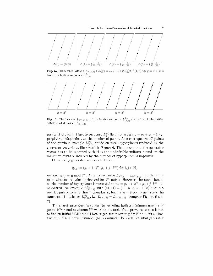
One way of constructing a MMD rank-1 lattice sequence is by taking a gen-erator vector g of a MMD rank-1 lattice Lbm,g and using it in Equation (2).For q ∈ N0 and a �xed m, each set of points {xq·bm , . . . , x(q+1)bm−1} ⊂ LΦb

g

is a copy of Lbm,g shifted by ∆(q) := Φb(q)b−mg [10]. The minimum distance

of all copies is identical, as dmin is shift invariant. For the example of LΦ2(1,3)

this structural property [9] is depicted in Figure 5. We now consider a two-dimensional generator vector g = (g1, g2) with gcd(n, g1, g2) = 1. Then all


∆(0) = (0, 0) ∆(1) = ( 116

, 316

) ∆(2) = ( 132

, 332

) ∆(3) = ( 332

, 932

)

Fig. 5. The shifted lattices L8,(1,3)+∆(q) = L8,(1,3)+Φ2(q)2−3(1, 3) for q = 0, 1, 2, 3

from the lattice sequence LΦ2(1,3).

n = 23 n = 24 n = 25 n = 26

Fig. 6. The lattices L2m,(1,3) of the lattice sequence LΦ2(1,3) started with the initial

MMD rank-1 lattice L8,(1,3).

points of the rank-1 lattice sequence LΦbg lie on at most nh = g1 + g2 − 1 hy-

perplanes, independent on the number of points. As a consequence, all pointsof the previous example LΦ2

(1,3) reside on three hyperplanes (induced by the

generator vector), as illustrated in Figure 6. This means that the generatorvector has to be modi�ed such that the undesirable uniform bound on theminimum distance induced by the number of hyperplanes is improved.

Considering generator vectors of the form

gi,j := (g1 + i · bm, g2 + j · bm) for i, j ∈ N0,

we have gi,j ≡ g mod bm. As a consequence Lbm,g = Lbm,gi,j, i.e. the mini-

mum distance remains unchanged for bm points. However, the upper boundon the number of hyperplanes is increased to nh = g1 + i · bm + g2 + j · bm− 1,as desired. For example LΦ2

(41,11) with (41, 11) = (1 + 5 · 8, 3 + 1 · 8) does notrestrict points to only three hyperplanes, but for n = 8 points generates thesame rank-1 lattice as LΦ2

(1,3), i.e. L8,(1,3) = L8,(41,11) (compare Figures 6 and

7).The search procedure is started by selecting both a minimum number of

points bmmin and maximum bmmax . First a search of the previous section is runto �nd an initial MMD rank-1 lattice generator vector g for bmmin points. Thenthe sum of minimum distances (6) is evaluated for each potential generator


d(3) = 8 = 8 d(4) = 10 < 16 d(5) = 26 < 32 d(6) = 58 < 65

d(7) = 74 < 137 d(8) = 250 < 277 d(9) = 362 < 580 d(10) = 362 < 1160

Fig. 7. Searching an MMD rank-1 lattice sequence for the initial lattice L23,(1,3)

(see Figure 6) and mmax = 7, yields LΦ2(41,11) with g5,1 = (1 + 5 · 23, 3 + 1 · 23) =

(41, 11). The gray lines show all possible hyperplanes. For each lattice of the rank-1lattice sequence we compare its minimum distance d(m) := dmin(Lbm,g)2bm to themaximum minimum distance that can be obtained by a single MMD rank-1 lattice.

vector gi,j in order to �nd the maximum, where the search range is determinedby

g1 + i · bmmin ≤ bmmax ⇒ i ≤ bmmax − g1

bmmin< bmmax−mmin and

g2 + j · bmmin ≤ bmmax ⇒ j ≤ bmmax − g2

bmmin< bmmax−mmin .

Due to symmetry, an obvious optimization is to bound the range of j bybmmax−mmin − i. Again, minimum distances are computed using the Gaussianbasis reduction. An example result of the search is illustrated in Figure 7,where minimum distances obtained by the rank-1 lattice sequence are com-pared to the distances that can be obtained by rank-1 lattices alone.

Approximate Search by Restricting the Search Space

In the second approach the search is not based on an initial MMD rank-1lattice. Instead we choose mmin = 1 and �x a value for mmax, looking for agenerator vector that maximizes Equation (6).

In order to accelerate the search process, the search space can be re-stricted using the same strategy as in the rasterization search algorithm for


d(1) = 2 = 2 d(2) = 5 < 9 d(3) = 26 = 26 d(4) = 65 < 85

d(5) = 113 < 261 d(6) = 701 < 810 d(7) = 2117 < 2522

Fig. 8. LΦ3(47,19) in base b = 3. For each lattice of the rank-1 lattice sequence we

compare its minimum distance d(m) := dmin(Lbm,g)2bm to the maximum minimumdistance that can be obtained by a single MMD rank-1 lattice.

rank-1 lattices (see Section 2.1). Then the search space is the union of therestricted search spaces for Lbm,g, 1 < m ≤ mmax. In experiments, the re-stricted search achieved the same results as the exhaustive computer searchfor nmax := bmmax ≤ 256 and b = 2, 3, 4, simultaneously reducing the run-timefrom O(n2

max log nmax) to O(√

nmax log nmax).We compare the two search approaches presented in this section by sum-

ming the minimum distances of the �rst bm points of each sequence

7∑m=2

d(m) =7∑

m=2

dmin(Lbm,g)2bm.

Although the second approach is more general than the �rst one, the latticesproduced by the sequence might not necessarily have the maximal possibleminimum distance for the corresponding n = bm points, which is assured atleast for the initial lattice in the �rst approach. Figure 8 shows the resultinglattice sequence for b = 3 and mmax = 7, while Table 1 shows the results ofthe numerical comparison. By de�nition for m = 2 the lattice of the sequenceLΦ3

(82,129) represents an MMD rank-1 lattice, whereas for m = 3 the rank-1

lattice of the sequence LΦ3(47,19) achieves the largest possible minimum distance

as well.


m d(m) �rst approach d(m) second approach

2 9 5

3 25 26

4 34 65

5 229 113

6 745 701

7 1033 2117

Σ 2075 3027

Table 1. Comparing the lattice sequences LΦ3(82,129) and LΦ3

(47,19) with respect tothe minimum distance of the �rst bm points of the lattice sequence for b = 3 and2 ≤ m ≤ 7. The initial MMD rank-1 lattice for LΦ3

(82,129) is given by L32,(1,3).

3 Search of Anisotropic Rank-1 Lattices to Approximate

Spectra

In many graphics applications the image functions exhibit a strong anisotropicbehavior in their Fourier spectrum. By constructing rank-1 lattices withknowledge of these functions the image quality can be improved. The Fouriertransform of the Shah function

XLn,g(x) :=∑p∈Zs

δ(x−B · p)

over the lattice Ln,g with basis B, where δ(x) is Dirac's delta function, yieldsanother Shah function over its dual lattice L⊥n,g [6]. This means that we candescribe the spectrum Sn,g of Ln,g by the fundamental Voronoi cell of thedual lattice L⊥n,g.We characterize the shape of this cell by two parameters,namely by its orientation −→ω L and by its width wL, which are computed bymeans of the basis B⊥ of L⊥n,g. Given a lattice basis B = (b1b2)t, where t

means transposed, the dual basis can be easily determined by B⊥ = (B−1)t.In order to assure that B⊥ spans the Delaunay triangulation and thus theVoronoi diagram, the dual basis has to be reduced, for example using theGaussian basis reduction. Let

v :={

b⊥1 + b⊥2 if b⊥1 · b⊥2 < 0b⊥2 − b⊥1 otherwise

be the diagonal of the basis cell spanned by b⊥1 and b⊥2 , such that v and b⊥1 orv and b⊥2 form a valid basis of the dual lattice as well. Then we approximatethe orientation of the fundamental Voronoi cell by

−→ω L := b⊥2 + v ={

2 · b⊥2 + b⊥1 if b⊥1 · b⊥2 < 02 · b⊥2 − b⊥1 otherwise.

(7)

The width wL of Sn,g is de�ned as the length of the shortest basis vectornormalized by the hexagonal bound l, i.e.


wL =||b⊥1 ||l · n

. (8)

Note that l · n also represents an upper bound on the maximized minimumdistance of the dual lattice, as the length of shortest vector in L⊥n,g correspondsto the length of the shortest vector in Ln,g scaled by n [4].

The spectrum Td,w, according to which we want to search the rank-1 lat-tice, is speci�ed by its main direction, i.e. orientation, d ∈ R2 and its widthw. The two-dimensional vector d and the scalar w are passed as an inputparameter to the lattice search by an application. The width w takes valuesin the range of [0, 1] and represents the measure of desired anisotropy. Themost anisotropic spectrum is denoted by w = 0, whereas w = 1 representsthe isotropic one. Note that we have to allow gi = 0, i = 1, 2 for the genera-tor vector in order to be able to approximate spectra aligned to axes of theCartesian coordinate system.

For n ∈ N the search algorithm steps through all distinct lattices. Thiscan be realized for example by using an n×n array, where the generator vec-tors of identical lattices are marked. Given any g ∈ [0, n)2, the set of vectorsyielding identical lattices is {k · g mod n : gcd(n, k) = 1, k = 1, . . . , n − 1}.After computing a Minkowski-reduced basis of the dual lattice, the orienta-tion and width of the fundamental Voronoi cell are determined according toEquations (7) and (8). Then the lattices are sorted with respect to |wL − w|.For the smallest di�erence we choose the lattice, whose orientation −→ω L bestapproximates the main direction d of Td,w. Thereby the similarity

sim =d · −→ω L

‖d‖ · ‖−→ω L‖

between those two vectors is measured by calculating the cosine of the anglebetween −→ω L and d. Figure 9 shows an example for anisotropic rank-1 latticeshaving n = 56 points, where the spectrum is speci�ed by d = (cos α, sinα)with α = 303◦ and the width varies from 0.1 to 1.0 in steps of 0.1. Using theGaussian basis reduction for the lattice basis search, the algorithm runs inO(n2 log n) time.

4 Weighted Norms

So far we considered rank-1 lattices only on the unit square. However, graphicsapplications often require arbitrary rectangular regions. Just selecting a corre-sponding region of the lattice de�ned in the entire real space and scaling it tothe unit square is not an option as this would destroy for example the neededperiodicity and complicate address computations in image applications. Wenow show how to extend our approximate search for isotropic and anisotropicrank-1 lattices to such regions.


b⊥1

−→ω

d

wL = 0.1, g = (27, 2)

b⊥1

−→ω

d

wL = 0.3, g = (13, 2)

b⊥1

−→ωd

wL = 0.5, g = (13, 1)

b⊥1

−→ωd

wL = 0.7, g = (8, 7)

b⊥1

−→ω

d

wL = 0.9, g = (5, 7)

b⊥1

−→ωd

wL = 1.0, g = (7, 4)

Fig. 9. Resulting spectra for a �xed direction d = (cos 303◦, sin 303◦) and widthvarying from 0.1 to 1.0.

Fig. 10. Searching on a rectangular domain. Left: MMD rank-1 lattice L512,(4,45)

in a domain of width-to-height ratio x : y = 4 : 1 in world coordinates. Right: Thesame lattice in the scaled basis with x : y = 1 : 1. The search region becomes anellipse.

All that needs to be done is considering the weighted norm ||Brxi|| in thede�nition of the minimum distance in Equation (4) instead of the Euclideannorm where Br describes the transformation of the unit square to the desiredregion. Note that as before the distance to the origin has to be computed withrespect to the unit torus.

Approximate Search for MMD rank-1 lattices

For the special case of scaled rectangular domains, i.e. Br = (br1b

r2) =

((x, 0)t(0, y)t), the rasterization search can be adapted easily. Therefore thelattice basis B has to be transformed into world coordinates before computing


its determinant, i.e. area A. For the �weighted� lattice basis Bw = Br ·B thearea of the basis cell is

A = |det Bw| = |det Br| · |det B| = x · yn

⇒ l =

√2 · x · yn ·√

3

in analogy to Equation (5).Since we perform the rasterization directly in the sheared basis, the short-

est vectors lie within an ellipse (see Figure 10). Its axes ax = ((n · l)/x, 0)t

and ay = (0, (n · l)/y)t result from transforming the circle axes ((n · l), 0)t and(0, (n · l))t into the sheared basis Br of the actual region.

As the rasterization runs in less than O(||ax||+ ||ay||), with ||ax||, ||ay|| ∈O(√

n), we still have a run-time complexity of O(√

n). Finally the Gaussianbasis reduction needs to be adapted to weighted norms in order to computethe minimum distance. For that purpose the only modi�cation consists inweighting the initial basis before performing the reduction steps. Thereforethe search algorithm maintains a run-time complexity of O(

√n log n).

Anisotropic Rank-1 Lattices

Using the algorithm from Section 3 with weighted norms only requires totransform the desired main direction d ∈ R2 into the sheared basis Br of thedesired domain.

5 Applications in Computer Graphics

The search algorithms from Section 2.1 allow one to �nd suitable generatorvectors for the graphics applications introduced in [3, 4] much faster. Here,we introduce two new applications of anisotropic rank-1 lattices.

5.1 Anti-Aliasing by Anisotropic Rank-1 Lattices

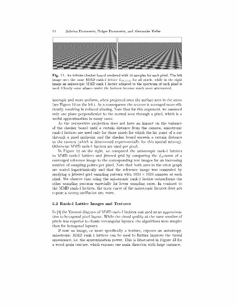
In graphics applications rank-1 lattices can be used to integrate the imagefunction over the pixels. By adapting the quadrature rule to the Fourier spec-trum of the image function in a way that more of the important frequenciesare captured, aliasing artifacts can be reduced. The improved anti-aliasing isillustrated by a comparison in Figure 11.

Given the algorithm from Section 3, an anisotropic MMD rank-1 latticeis speci�ed by the main direction d and the width w. We globally assumemaximum anisotropy by �xing w = 0. The main direction d is determinedby projecting the normal of the �rst object intersected by a ray through thecenter of a pixel onto the image plane and normalizing the resulting vector.This way the samples from the anisotropic rank-1 lattice in the pixel become


Fig. 11. An in�nite checker board rendered with 16 samples for each pixel. The leftimage uses the same MMD rank-1 lattice L16,(1,4) for all pixels, while in the rightimage an anisotropic MMD rank-1 lattice adapted to the spectrum of each pixel isused. Clearly some aliases under the horizon become much more attenuated.

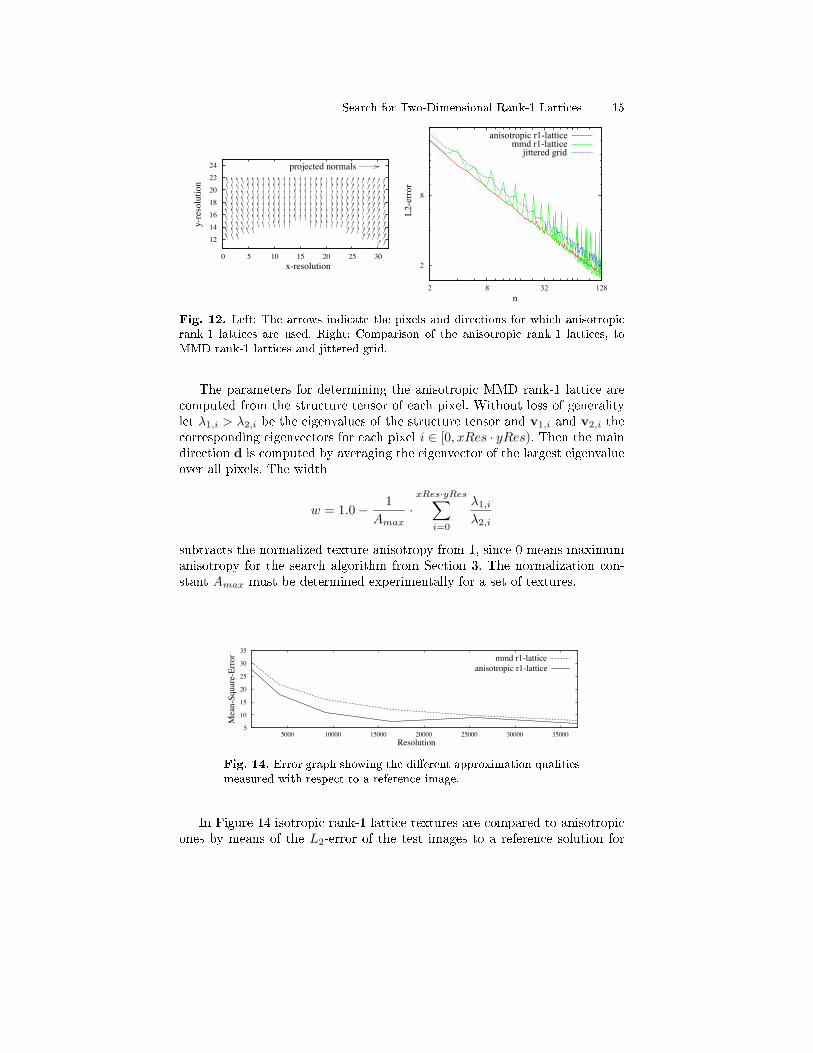
isotropic and more uniform, when projected onto the surface seen in the scene(see Figure 12 on the left). As a consequence the texture is averaged more e�-ciently, resulting in reduced aliasing. Note that for this argument, we assumedonly one plane perpendicular to the normal seen through a pixel, which is auseful approximation in many cases.

As the perspective projection does not have an impact on the varianceof the checker board until a certain distance from the camera, anisotropicrank-1 lattices are used only for those pixels for which the hit point of a raythrough a pixel midpoint and the checker board exceeds a certain distanceto the camera (which is determined experimentally for this special setting).Otherwise MMD rank-1 lattices are used per pixel.

In Figure 12 on the right, we compared the anisotropic rank-1 latticesto MMD rank-1 lattices and jittered grid by computing the L2-norm of aconverged reference image to the corresponding test images for an increasingnumber of sampling points per pixel. Note that both axes in the error graphare scaled logarithmically and that the reference image was computed byapplying a jittered grid sampling pattern with 1024 × 1024 samples at eachpixel. We observe that using the anisotropic rank-1 lattice outperforms theother sampling patterns especially for lower sampling rates. In contrast tothe MMD rank-1 lattices, the error curve of the anisotropic lattices does notexpose a strong oscillation any more.

5.2 Rank-1 Lattice Images and Textures

In [4] the Voronoi diagram of MMD rank-1 lattices was used as an approxima-tion to hexagonal pixel layout. While the visual quality at the same number ofpixels was superior to classic rectangular layouts, the algorithms were simplerthan for hexagonal layouts.

If now an image, or more speci�cally a texture, exposes an anisotropy,anisotropic MMD rank-1 lattices can be used to further improve the visualappearance, i.e. the approximation power. This is illustrated in Figure 13 fora wood grain texture, which exposes one main direction with large variance.


12 14 16 18 20 22 24

0 5 10 15 20 25 30

y-re

solu

tion

x-resolution

projected normals

2

8

2 8 32 128

L2-

erro

r

n

anisotropic r1-latticemmd r1-lattice

jittered grid

Fig. 12. Left: The arrows indicate the pixels and directions for which anisotropicrank-1 lattices are used. Right: Comparison of the anisotropic rank-1 lattices, toMMD rank-1 lattices and jittered grid.

The parameters for determining the anisotropic MMD rank-1 lattice arecomputed from the structure tensor of each pixel. Without loss of generalitylet λ1,i > λ2,i be the eigenvalues of the structure tensor and v1,i and v2,i thecorresponding eigenvectors for each pixel i ∈ [0, xRes · yRes). Then the maindirection d is computed by averaging the eigenvector of the largest eigenvalueover all pixels. The width

w = 1.0− 1Amax

·xRes·yRes∑

i=0

λ1,i

λ2,i

subtracts the normalized texture anisotropy from 1, since 0 means maximumanisotropy for the search algorithm from Section 3. The normalization con-stant Amax must be determined experimentally for a set of textures.

5

10

15

20

25

30

35

5000 10000 15000 20000 25000 30000 35000

Mea

n-Sq

uare

-Err

or

Resolution

mmd r1-latticeanisotropic r1-lattice

Fig. 14. Error graph showing the di�erent approximation qualitiesmeasured with respect to a reference image.

In Figure 14 isotropic rank-1 lattice textures are compared to anisotropicones by means of the L2-error of the test images to a reference solution for


Fig. 13. Magni�cations of the highlighted squares in the texture on the left repre-sented on the regular grid, MMD rank-1 lattice, and anisotropic rank-1 lattice by16384 pixels each. Note that for the anisotropic rank-1 lattice the mean square error(MSE) to the high resolution reference on the right is about half of the regular andMMD rank-1 lattice.

an increasing number of lattice points for the source image of Figure 13. Ascan be seen from the error graph, the anisotropic rank-1 lattice textures aresuperior, as they are able to capture even small details, which are lost in theisotropic case.

6 Conclusions

We introduced algorithms that e�ciently search for generator vectors of rank-1lattices and sequences with important new applications in computer graphics.Useful results were obtained for both image synthesis and representation.Future research will concentrate on applications of rank-1 lattice sequencesand the fast search of generator vectors for the anisotropic case.

Acknowledgement. The authors would like to thank mental images GmbH for sup-port and funding of this research.

References

1. Conway, J., Sloane, N., Bannai, E.: Sphere-packings, Lattices, and Groups.Springer-Verlag New York, Inc. (1987)

2. Cools, R., Reztsov, A.: Di�erent quality indexes for lattice rules. Journal ofComplexity 13(2), 235�258 (1997)

3. Dammertz, H., Keller, A., Dammertz, S.: Simulation on rank-1 lattices. In:A. Keller, S. Heinrich, H. Niederreiter (eds.) Monte Carlo and Quasi-MonteCarlo Methods 2006, pp. 205�216. Springer (2008)


4. Dammertz, S., Keller, A.: Image synthesis by rank-1 lattices. In: A. Keller,S. Heinrich, H. Niederreiter (eds.) Monte Carlo and Quasi-Monte Carlo Methods2006, pp. 217�236. Springer (2008)

5. Dieter, U.: How to Calculate Shortest Vectors in a Lattice. Math. Comp.29(131), 827�833 (1975)

6. Entezari, A., Dyer, R., Möller, T.: From sphere packing to the theory of optimallattice sampling. In: T. Möller, B. Hamann, R. Russell (eds.) MathematicalFoundations of Scienti�c Visualization, Computer Graphics, and Massive DataExploration. Springer (2009)

7. Fincke, U., Pohst, M.: Improved Methods for Calculating Vectors of ShortLength in a Lattice, Including a Complexity Analysis. Math. Comp. 44, 463�471(1985)

8. Foley, J., van Dam, A., Feiner, S., Hughes, J.: Computer Graphics, Principlesand Practice, 2nd Edition in C. Addison-Wesley (1996)

9. Hickernell, F., Hong, H.: Computing multivariate normal probabilities usingrank-1 lattice sequences. In: G. Golub, S. Lui, F. Luk, R. Plemmons (eds.)Proceedings of the Workshop on Scienti�c Computing (Hong Kong), pp. 209�215. Springer (1997)

10. Hickernell, F., Hong, H., L'Ecuyer, P., Lemieux, C.: Extensible lattice sequencesfor quasi-Monte Carlo quadrature. SIAM J. Sci. Comput. 22, 1117�1138 (2001)

11. Kannan, R.: Algorithmic Geometry of Numbers. Annual Reviews in ComputerScience 2, 231�267 (1987)

12. Knuth, D.: The Art of Computer Programming Vol. 2: Seminumerical Algo-rithms. Addison Wesley (1981)

13. L'Ecuyer, P.: Tables of Linear Congruential Generators of Di�erent Sizes andGood Lattice Structure. Math. Comput. 68(225), 249�260 (1999)

14. L'Ecuyer, P., Couture, R.: An Implementation of the Lattice and Spectral Testsfor Multiple Recursive Linear Random Number Generators. INFORMS Journalon Computing 9(2), 206�217 (1997)

15. L'Ecuyer, P., Lemieux, C.: Variance Reduction via Lattice Rules. Manage. Sci.46(9), 1214�1235 (2000)

16. Martinet, J.: Perfect Lattices in Euclidean Spaces. Springer-Verlag (2003)17. Niederreiter, H.: Random Number Generation and Quasi-Monte Carlo Methods.

SIAM, Philadelphia (1992)18. Rote, G.: Finding a Shortest Vector in a Two-Dimensional Lattice Modulo m.

Theoretical Computer Science 172(1�2), 303�308 (1997)19. Siegel, C.: Lectures on Geometry of Numbers. Springer-Verlag (1989)20. Sloan, I., Joe, S.: Lattice Methods for Multiple Integration. Clarendon Press,

Oxford (1994)

Documents

E cient Search for wTo-Dimensional Rank-1 Lattices with ... · E cient Search for wTo-Dimensional Rank-1 Lattices with Applications in Graphics Sabrina Dammertz 1, Holger Dammertz