Efficient Production and Factor Allocation -

Economic Planning and the Price Systems :

Analytic Production Possibility Curves, Transformation

Functions, Pareto Efficient Factor Allocations, Revenue

Functions, General Equilibrium and Comparative Costs

Bjarne S. Jensena,1, Jacopo Zottib , Jens Martin Jensenc

aSociology, Environmental, and Business Economics, University of Southern Denmark

bDepartment of Political and Social Sciences, University of Trieste, Italy

cMartin Pointing Devices, Virum, Denmark

Abstract

Reviewing aspects of Transformation Functions, Production Possibility Cur-ves, and Factor Contract Curves, this paper presents explicit (parametric)Transformation Functions. Moreover, analytic production possibility graphsare provided for implicit transformation functions. Hence Production Pos-sibility Frontiers are now analytically stated for any Cobb-Douglas sector(CD) technology parameters and any factor endowments of labor and capital.’Core theorems’ of international trade are unified, extended, illustrated byanalytic (parametric) representation of all Pareto efficient factor allocations.The theorems from analytic transformation and dual revenue functions arecompared with general equilibrium solutions of autarky and comparative cost(trade pattern predictions) for two trading economies with any CD sectortechnologies, consumer preferences and endowments of labor and capital.

Keywords:Technology, Allocation, Pareto Efficiency, General Equilibrium, TradeJEL Classification: B21, D24, D51, D61, F11, O41

1Corresponding author, email: bsj@sam.sdu.dkSEBE, University of Southern Denmark,Niels Bohrs Alle 9, 6700 Esbjerg, Denmark.

Preprint submitted to ?? June 14, 2018

2

1. Introduction

Production possibility frontiers (PPF) show alternative combinations ofoutputs that can be obtained, when the given endowments are allocated ef-ficiently. Two-dimensional diagrams of concave PPF curves prevail in manyfields of economic analysis. The PPF curves are obtained from transfor-mation functions that reflect technology assumptions and the endowments.Despite numerous applications of PPC curves, we have so far in the literaturenever seen an explicit transformation function. Our purpose is to close thegap by showing explicit Transformation Functions - rigorously derived fromthe Pareto efficiency conditions in factor space and output space.

The ”production indifference, transformation” curve was originated byLeontief, when in production (output) diagrams, he replaced the assumptionof ”constant opportunity cost” with a ”production curve concave toward theaxes”, Leontief (1933, p.405). However, the concave PPF curve is a ”top of alarge iceberg”, representing the result of complicated economic processes andrelations, by which given endowments are optimally allocated between sectorsin accordance with marginal productivity conditions that ensure maximumof one output for any preassigned amounts of the second output. Stolperand Samuelson (1941, p.68) established the connection between optimal fac-tor allocations, factor contract curves (FFC), and maximal output curves(PPC). Cf. ”contract curve, utility indifference curves touch” (Edgeworth1881, p.36), Black (1957), Hsiao (1971, p.920). Computer programs hasbeen set up to chart transformation curves for some of our CD parameters,Johnson (1966, p.693); adopting a factor endowment ratio of unity impliesserious loss of generality for shapes of PPF curves, demonstrated in Fig. 5.

Our main results are stated in Lemma 1-2, giving explicit parametricFactor Contract Curves (FCC) and Factor Allocation Curves, andTheorem 1-2, with analytic Production Possibility Curves, (PPC), andparametric Transformation Functions with solutions seen in Fig. 1-7.

With our Lemmas and Theorems, FCC and PPC curves can be generatedfor any CD parameters and factor endowments that may be used to studyspecific parameter impacts on autarky and international economic equilibria.

We proceed axiomatically in exposition and sections. Section 2 givesthe general framework of endowments and technology of autarky economies;Pareto efficiency conditions establish FCC and FAC curves in factor space.Section 3 links FCC with PCC in analytic forms. Section 4 gives explicittransformation functions and duals. Section 5 shows general equilibrium.

3

2. Endowments, Sector Allocations, Technologies, and Efficiency

2.1. Two-Sector, Two-Factor, Two-Country Framework

There are two countries in the world, A and B. These countries mayproduce two consumer goods (sectors), i = 1, 2, which are fully homogeneousthroughout the world. In both sectors, they are using two primary productionfactors, labour and capital. Labour endowment in country J = A,B is LJ ,while capital endowment is KJ ; its factor proportion (endowment ratio) is,kJ = KJ/LJ . It is generally assumed that both factors are fully employed :

K1J +K2J = KJ , L1J + L2J = LJ ; kiJ ≡ KiJ/LiJ , i = 1, 2 (1)

kJ = KJ/LJ = λL1Jk1J + λL2J

k2J ; k2J = [kJ − λL1Jk1J ]/[1− λL1J

], J = A,B (2)

λL1J≡ L1J/LJ = [kJ − k2J ]/[k1J − k2J ] , λL2J

= 1−λL1J; i = 1, 2 , J = A,B (3)

λK1J≡ K1J/KJ = [k1J/kJ ]λL1J

, λK2J= 1− λK1J

; i = 1, 2 , J = A,B (4)

where λLiJ , λKiJ , are the shares -fractions - of labour (capital) in country Jallocated to sector (i); kiJ is the capital-labour ratio of sector (i), country J .Diversification, production of both goods, is equivalent the inequalities,

0 < λL1J< 1 : k1J > kJ > k2J or k1J < kJ < k2J , J = A,B (5)

Technology exhibits constant returns to scale in both countries, J = A,B. Forsector, i = 1, 2, and standard Cobb-Douglas (CD) parameter specifications,

YiJ = FiJ(LiJ ,KiJ) = γiJL1−aiJiJ KaiJ

iJ = LJλLiJyiJ ; yiJ = γiJkaiJiJ , i = 1, 2 (6)

YiJ : non-joint product of sector (i) in country J - with sector average laborproductivity, yiJ ≡ YiJ/LiJ , capital-labor ratio, kiJ ≡ KiJ/LiJ , the capitalintensity parameter : aiJ , 0 < aiJ < 1, and 1− aiJ is the labour intensity.

Sector (industry) technologies for YiJ with σi =∞ , i = 1, 2, are :

YiJ = FiJ(LiJ ,KiJ) = γiJ [(1− aiJ)LiJ + aiJKiJ ] = LJλLiJyiJ ; i = 1, 2 (7)

The construction of the production possibilities frontier (PPF boundary)from the resource endowments above and the technological opportunities of-fered by two industry production functions is one main objective. The fron-tier is obtained by using the Pareto efficiency principle (society unanimouslyprefers more of any good, if no amounts of other goods are diminished). Theexistence and concavity conditions for PPF boundary curves are well-known.

The basic problem: Can a PPF curve of Pareto efficient values (Y1J , Y2J),be given by one algebraic equation for an explicit transformation function ?

4

2.2. Pareto Economic Efficiency in Production of Any Factor EndowmentsFor country J , the production possibility frontier (PPF) is defined as a

locus of points in output space, (Y1J , Y2J), which are Pareto optimal : for anyY1J , the maximum Y2J obtained by any given endowments, (LJ , KJ), viceversa. The locus (PPF) is typically described by transformation functions

in implicit, TJ or explicit functional form TJ , Samuelson (1983,p.230), Hicks(1946,p.319), Silberberg & Suen (2001,p.541), Mass-Colell et al. (1995.p.128),

TJ(Y1J , Y2J ; LJ ,KJ) = 0 ⇔ Y2J = TJ(Y1J ; LJ ,KJ) ; Y2J = TJ(Y1J ; LJ ,KJ) (8)

Differentiable transformation functions (8) imply standard efficiency condi-

tions. Discussion of Transformation Functions, TJ or TJ has been confined toessential marginal (derivative) properties in qualitative form. One goal is toobtain quantitative explicit (parametric) expressions of TJ(Y1J ;LJ , KJ), i.e.,besides LJ , KJ to see TJ (8) specified completely by technology parameters :

γiJ , aiJ , i = 1, 2, (6). We shall see graphs in analytic form of : TJ , TJ , (8).Apart from the concavity and homogeneity (degree one) properties

of transformation functions, (8), the actual shape of the PPF point set(Y1J , Y2J), were puzzling in many numerical simulations with graphics, John-son (1966), Scarth and Warne (1973). Our analytic expressions of the CDPPF graph, Y2J = TJ(Y1J ;LJ , KJ) resolve the fundamental questions involved.

The efficient factor allocation of labor and capital between the two sectorsimposes a common marginal rate of factor substitution, (MRS ), of labor andcapital (the ratio of marginal productivities of labor and capital) with (6):

dK1J

dL1J=∂F1J/∂L1J

∂F1J/∂K1J=

1− a1Ja1J

k1J =1− a2Ja2J

k2J =∂F2J/∂L2J

∂F2J/∂K2J=dK2J

dL2J(9)

An alternative, equivalent efficiency condition to (9) in finding the maximumpoints (frontier) of outputs is to impose a common marginal rate of transfor-mation (MRT) of outputs (ratio of marginal products) for both factors:

dY2JdY1J

=∂F2J/∂K2J

∂F1J/∂K1J=γ2Jγ1J

a2Ja1J

ka2J−12J

ka1J−11J

=γ2Jγ1J

1− a2J1− a1J

ka2J2J

ka1J1J

=∂F2J/∂L2J

∂F1J/∂L1J=dY2JdY1J

(10)From (9), we get, 0 < aiJ < 1 , i = 1, 2 ; AJ > 0 ; a1J ≷ a2J : AJ ≷ 1

k1J

k2J

=a1J (1− a2J)

a2J (1− a1J)= AJ ; AJ−1 =

a1J − a2J

a2J (1− a1J); 1−AJ =

a2J − a1J

a2J (1− a1J)(11)

MRT requirement (10) gives the same fundamental equation (11); but MRTare affected by γiJ . Pareto efficient k1J , k2J change, but maintain a propor-tionality relation, AJ - hence both rise or fall together to keep proportionality.

5

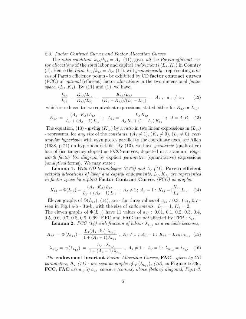
2.3. Factor Contract Curves and Factor Allocation CurvesThe ratio condition, k1J/k2J = AJ , (11), gives all the Pareto efficient sec-

tor allocations of the total labor and capital endowments (LJ , KJ) in Country(J). Hence the ratio, k1J/k2J = AJ , (11), will geometrically - representing a lo-cus of Pareto efficiency points - be exhibited by CD factor contract curves(FCC) of optimal (efficient) factor allocations in the two-dimensional factorspace, (LJ , KJ). By (11) and (1), we have,

k1J

k2J

=K1J/L1J

K2J/L2J

=K1J/L1J

(KJ −K1J)/(LJ − L1J)= AJ , a1J 6= a2J (12)

which is reduced to two equivalent expressions, stated either for K1J or L1J :

K1J =(AJ ·KJ)L1J

LJ + (AJ − 1)L1J

; L1J =LJ K1J

AJ KJ + (1−AJ)K1J

; J = A,B (13)

The equation, (13) - giving (K1J) by a ratio in two linear expressions in (L1J)- represents, for any size of the constants, (AJ 6= 1), (KJ 6= 0), (LJ 6= 0), rect-angular hyperbolas with asymptotes parallel to the coordinate axes, see Allen(1938, p.74) on hyperbola details. By (13), we have geometric (qualitative)loci of (iso-tangency slopes) as FCC-curves, depicted in a standard Edge-worth factor box diagram by explicit parametric (quantitative) expressions(analytical forms). We may state :

Lemma 1. With CD technologies (6-62) and AJ (11), Pareto efficientsectoral allocations of labor and capital endowments, LJ , KJ, are representedin factor space by explicit Factor Contract Curves (FCC) as graphs:

K1J = Φ(L1J) =(AJ ·KJ)L1J

LJ + (AJ − 1)L1J

, AJ 6= 1 ; AJ = 1 : K1J = [KJ

LJ]L1J (14)

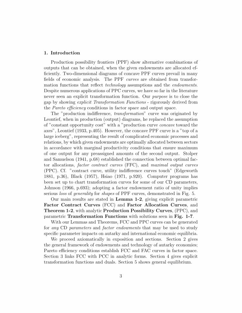
Eleven graphs of Φ(L1J), (14), are - for three values of a1J : 0.3 , 0.5 , 0.7 -seen in Fig.1 a-b - 3 a-b, with the size of endowments: LJ = 1, KJ = 2.The eleven graphs of Φ(L1J) have 11 values of a2J : 0.01, 0.1, 0.2, 0.3, 0.4,0.5, 0.6, 0.7, 0.8, 0.9, 0.99. FFC and FAC are not affected by TFP : γiJ .

Lemma 2. FCC (14) with fraction of labour λL1Jas a variable becomes,

K1J = Φ (λL1J) =

LJ(AJ · kJ) λL1J

1 + (AJ − 1)λL1J

, AJ 6= 1 ; AJ = 1 : K1J = LJ kJλL1J(15)

λK1J= ϕ (λL1J

) =AJ · λL1J

1 + (AJ − 1)λL1J

, AJ 6= 1 ; AJ = 1 : λK1J= λL1J

(16)

The endowment invariant Factor Allocation Curves, FAC - given by CDparameters, AJ (11) - are seen as graphs of ϕ (λL1J

), (16), in Figure 1c-3c.FCC, FAC are a1J ≷ a2J concave (convex) above (below) diagonal, Fig.1-3.

6

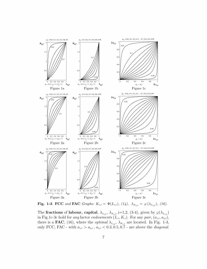
Figure 1a Figure 1b Figure 1c

Figure 2a Figure 2b Figure 2c

Figure 3a Figure 3b Figure 3c

Fig. 1-3. FCC and FAC Graphs: K1J = Φ(L1J), (14), λK1J= ϕ (λL1J

), (16).

The fractions of labour, capital, λLiJ , λKiJ , i=1,2, (3-4), given by ϕ(λL1J)

in Fig.1c-3c hold for any factor endowments (LJ , KJ). For any pair, (a1J , a2J),there is a FAC, (16), where the optimal λLiJ , λKiJ are located. In Fig. 1-3,only FCC, FAC - with a1J > a2J , a2J < 0.3, 0.5, 0.7 - are above the diagonal.

7

3. Factor Contract Curves and Production Possibility Curves

Lemma 1 gave Pareto efficient (LiJ , KiJ). By formula (14), (2), cf. (11),Lemma 3. Pareto efficient capital-labor ratios with λL1J

as variable are:

k1J =AJ · kJ

1 + (AJ − 1)λL1J

; k2J =kJ

1 + (AJ − 1)λL1J

; AJ = 1 : kiJ = kJ (17)

Theorem 1A. The allocation fraction of labour - λL1J- used as a single

(”parameter”, auxiliary) variable, 0 ≤ λL1J≤ 1, along any FCC curve, give

by (17) the Pareto efficient values of other variables, (15-16), (9-10), (6):

dKiJ

dLiJ= − 1− a2J

a2Jk2J = − 1− a2J

a2J

kJ1 + (AJ − 1)λL1J

; i = 1, 2 (18)

The equation (18) gives the MRS of labor and capital - slope at common tangencypoints of the sector isoquants - along the FCC curves (14) in (LJ ,KJ), Fig.1-3.

dY2JdY1J

= −γ2Jγ1J

a2Ja1J

ka2J−12J

ka1J−11J

= −γ2Jγ1J

a2Ja1J

A1−a1JJ

[ kJ1 + (AJ − 1)λL1J

]a2J−a1J (19)

The equation (19) gives the MRT of the outputs - the tangent slopes alongplanar production possibility curves, PPC, in the commodity space (Y1J , Y2J).The analytic production possibility arcs (oriented curves), 0 ≤ λL1J

≤ 1, ofPPC are, (17), (6), represented (”parametric”) by two functions/equations:

Y1J = LJ γ1J λL1J

[ AJ kJ1 + (AJ − 1)λL1J

]a1J ≡ LJ h1(λL1J; kJ) (20)

Y2J = LJ γ2J (1− λL1J)[ kJ1 + (AJ − 1)λL1J

]a2J ≡ LJ h2(λL1J; kJ) (21)

E (Y2J , Y1J) =dY2JdY1J

Y1JY2J

= − a2Ja1J

AJ

λL1J

1− λL1J

= − 1− a2J1− a1J

λL1J

1− λL1J

(22)

Generally - for any technology parameters : γiJ , aiJ , i = 1, 2, (6), and anyendowments, LJ , KJ - equations (20-21) link by λL1J

via Lemma 3, (17), allPareto efficient (optimal) factor allocations in factor space (LJ , KJ) - alongany factor contract curve, e.g., the particular FCC curves , as well theparametrically shifting FCC curves in Figures 1-3 - to their correspondingmaximum points (frontier) in the output space (Y1J ,Y2J). The set ofthe ordered numbers (Y1J , Y2J) given by (20-21), 0 ≤ λL1J

≤ 1, is theproduction possibility curve (PPC) in output space, Figures 4-6.

Thus, (20-21), 0 ≤ λL1J≤ 1 , do represent the graph of TJ (8), for the

production possibility curve (PPC) in output space. This PPC (produc-tion frontier, Cobb-Douglas envelope ) has an elasticity (22) that is changingalong PPC - but (22) is endowment invariant; MRT is constant for rays.

8

Along the concave (convex) curves, FCC, FAC, Fig.1-3 , a1J ≷ a2J ,with k1J ≷ k2J , λK1J

≷ λK2J, λL1J

≶ λL2J, above (below) the diagonal, the

common MRS (18) is numerically falling (rising) : declining (rising) from[(1 − a2J)/a2J ] kJ to [(1 − a1J)/a1J ] kJ - cf. (26-27) below. Along any FCC,FAC, λK1J

, λL1Jare both increasing.

Theorem 1B. Along any FCC, common MRS = ωJ (18),(9),(3),(11) give,

ωJ =∂F1J/∂L1J

∂F1J/∂K1J=

∂F2J/∂L2J

∂F2J/∂K2J=

1− a2Ja2J

kJ1 + (AJ − 1)λL1J

, J = A,B (23)

kiJ = kiJ(ωJ) =aiJ

1− aiJωJ , i = 1, 2 , J = A,B (24)

λL1J(ωJ ; kJ) =

kJ/k2J(ωJ)− 1

k1J(ωJ)/k2J(ωJ)− 1=

(1− a1J)(1− a2J)

a1J − a2JkJωJ− 1

AJ − 1(25)

For a given endowment ratio (kJ) - upper boundary (ωJ), lower boundary(ωJ) - of the common ωJ along any FCC are evidently given by (24) as,

a1J > a2J : ωJ =1− a1J

a1J

kJ 5 ωJ(kJ) 51− a2J

a2J

kJ = ωJ (26)

a1J < a2J : ωJ =1− a2J

a2J

kJ 5 ωJ(kJ) 51− a1J

a1J

kJ = ωJ (27)

Along any PPC, common MRT = pJ (19) is related to MRS (23) by (24):

MRT = pJ =γ2Jγ1J

a2Ja1J

ka2J−12J

ka1J−11J

=γ2J

γ1J

· aa2J2J (1− a2J)1−a2J

aa1J1J (1− a1J)1−a1J· ωa2J−a1JJ (28)

≡ γ2J

γ1J

AJ ωa2J−a1JJ ≡ φJ(ωJ) ; E (MRT,MRS ) = a2J − a1J (29)

HenceωJ = φ−1J (pJ) : λL1J

(pJ ; kJ) =[1− a1J ][1− a2J ]

a1J − a2J

[γ1J pJγ2J AJ

] 1a2J−a1J

kJ−1

AJ − 1(30)

For a given endowment ratio (kJ) - upper boundary (pJ), lower boundary(p

J) - of the common pJ along any PCC are by (26-29) derived to become:

pJ

=γ2J

γ1J

AJ

[1− a2J

a2J

kJ

]a2J−a1J5 pJ(kJ) 5

γ2J

γ1J

AJ

[1− a1J

a1J

kJ

]a2J−a1J= pJ (31)

pJ

and p J are slopes of PPC at endpoints with output Y1J = 0 and Y2J = 0.The MRT- MRS correspondence (29) applies to any PCC in Fig. 4-6.The relations with Pareto efficiency - kiJ = kiJ(ωJ), (24), and pJ = φJ(ωJ),(29) - are explicitly (parametric) exhibited for, a1J ≷ a2J, in Fig. 7a - 7b.Along any PPC from Y1J = 0 to Y2J = 0, slope (19): MRT= pJ= φJ(ωJ),(29), is always - a1J ≷ a2J - monotonic increasing - which is shown graph-ically by Pareto efficient factor reallocation from A to B in Fig. 7a - 7b.

9

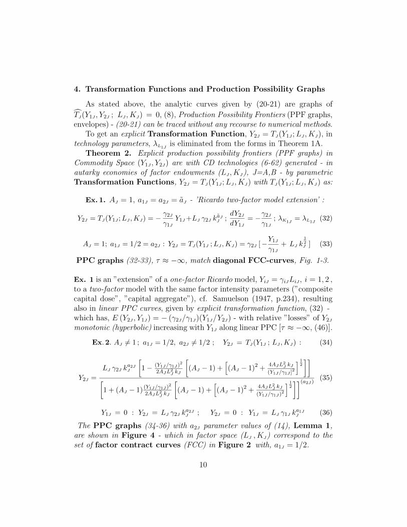
4. Transformation Functions and Production Possibility Graphs

As stated above, the analytic curves given by (20-21) are graphs of

TJ(Y1J , Y2J ; LJ , KJ) = 0, (8), Production Possibility Frontiers (PPF graphs,envelopes) - (20-21) can be traced without any recourse to numerical methods.

To get an explicit Transformation Function, Y2J = TJ(Y1J ;LJ , KJ), intechnology parameters, λL1J

is eliminated from the forms in Theorem 1A.Theorem 2. Explicit production possibility frontiers (PPF graphs) in

Commodity Space (Y1J , Y2J) are with CD technologies (6-62) generated - inautarky economies of factor endowments (LJ , KJ), J=A,B - by parametricTransformation Functions, Y2J = TJ(Y1J ;LJ , KJ) with TJ(Y1J ;LJ , KJ) as:

Ex. 1. AJ = 1, a1J = a2J = aJ - ’Ricardo two-factor model extension’ :

Y2J = TJ(Y1J ;LJ ,KJ) = − γ2Jγ1J

Y1J+LJ γ2J kaJJ ;

dY2JdY1J

= −γ2Jγ1J

; λK1J= λL1J

(32)

AJ = 1; a1J = 1/2 = a2J : Y2J = TJ(Y1J ;LJ ,KJ) = γ2J [−Y1Jγ1J

+ LJ k12J ] (33)

PPC graphs (32-33), τ ≈ −∞, match diagonal FCC-curves, Fig. 1-3.

Ex. 1 is an ”extension” of a one-factor Ricardo model, YiJ = γiJLiJ , i = 1, 2 ,to a two-factor model with the same factor intensity parameters (”compositecapital dose”, ”capital aggregate”), cf. Samuelson (1947, p.234), resultingalso in linear PPC curves, given by explicit transformation function, (32) -which has, E (Y2J , Y1J) = − (γ2J/γ1J)(Y1J/Y2J) - with relative ”losses” of Y2Jmonotonic (hyperbolic) increasing with Y1J along linear PPC [τ ≈ −∞, (46)].

Ex.2. AJ 6= 1 ; a1J = 1/2, a2J 6= 1/2 ; Y2J = TJ(Y1J ; LJ ,KJ) : (34)

Y2J =

LJ γ2J ka2JJ

[1− (Y1J/γ1J )

2

2AJL2J kJ

[(AJ − 1) +

[(AJ − 1)2 +

4AJL2J kJ

(Y1J/γ1J ]2

] 12

]][1 + (AJ − 1) (Y1J/γ1J )

2

2AJL2J kJ

[(AJ − 1) +

[(AJ − 1)2 +

4AJL2J kJ

(Y1J/γ1J )2

] 12

]](a2J ) (35)

Y1J = 0 : Y2J = LJ γ2J ka2JJ ; Y2J = 0 : Y1J = LJ γ1J k

a1JJ (36)

The PPC graphs (34-36) with a2J parameter values of (14), Lemma 1,are shown in Figure 4 - which in factor space (LJ , KJ) correspond to theset of factor contract curves (FCC) in Figure 2 with, a1J = 1/2.

10

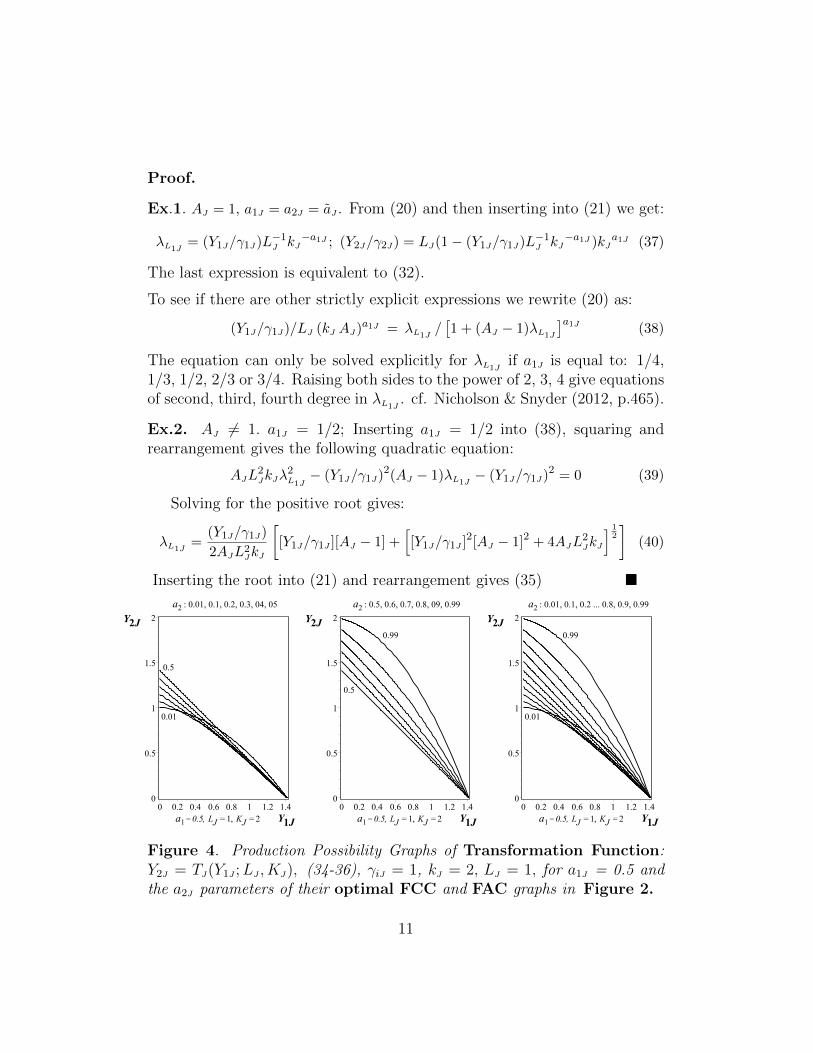
Proof.

Ex.1. AJ = 1, a1J = a2J = aJ . From (20) and then inserting into (21) we get:

λL1J= (Y1J/γ1J)L−1J kJ

−a1J ; (Y2J/γ2J) = LJ(1− (Y1J/γ1J)L−1J kJ−a1J )kJ

a1J (37)

The last expression is equivalent to (32).

To see if there are other strictly explicit expressions we rewrite (20) as:

(Y1J/γ1J)/LJ (kJ AJ)a1J = λL1J/[1 + (AJ − 1)λL1J

]a1J (38)

The equation can only be solved explicitly for λL1Jif a1J is equal to: 1/4,

1/3, 1/2, 2/3 or 3/4. Raising both sides to the power of 2, 3, 4 give equationsof second, third, fourth degree in λL1J

. cf. Nicholson & Snyder (2012, p.465).

Ex.2. AJ 6= 1. a1J = 1/2; Inserting a1J = 1/2 into (38), squaring andrearrangement gives the following quadratic equation:

AJL2JkJλ

2L1J− (Y1J/γ1J)2(AJ − 1)λL1J

− (Y1J/γ1J)2 = 0 (39)

Solving for the positive root gives:

λL1J=

(Y1J/γ1J)

2AJL2JkJ

[[Y1J/γ1J ][AJ − 1] +

[[Y1J/γ1J ]2[AJ − 1]2 + 4AJL

2JkJ

] 12

](40)

Inserting the root into (21) and rearrangement gives (35) �

Figure 4. Production Possibility Graphs of Transformation Function:Y2J = TJ(Y1J ;LJ , KJ), (34-36), γiJ = 1, kJ = 2, LJ = 1, for a1J = 0.5 andthe a2J parameters of their optimal FCC and FAC graphs in Figure 2.

11

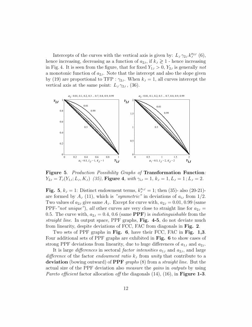
Intercepts of the curves with the vertical axis is given by: LJ γ2J ka2JJ (6),

hence increasing, decreasing as a function of a2J , if kJ ≷ 1 - hence increasingin Fig. 4. It is seen from the figure, that for fixed Y1J > 0, Y2J is generally nota monotonic function of a2J . Note that the intercept and also the slope givenby (19) are proportional to TFP : γ2J . When kJ = 1, all curves intercept thevertical axis at the same point: LJ γ2J , (36).

Figure 5. Production Possibility Graphs of Transformation Function:Y2J = TJ(Y1J ;LJ , KJ) (35), Figure 4, with γiJ = 1, kJ = 1, LJ = 1 ;LJ = 2.

Fig. 5, kJ = 1: Distinct endowment terms, kaiJJ = 1; then (35)- also (20-21)-are formed by AJ (11), which is ”symmetric” in deviations of aiJ from 1/2.Two values of a2J give same AJ . Except for curve with, a2J = 0.01, 0.99 (samePPF-”not unique”), all other curves are very close to straight line for a2J =0.5. The curve with, a2J = 0.4, 0.6 (same PPF) is indistinguishable from thestraight line. In output space, PPF graphs, Fig. 4-5, do not deviate muchfrom linearity, despite deviations of FCC, FAC from diagonals in Fig. 2.

Two sets of PPF graphs in Fig. 6, have their FCC, FAC in Fig. 1,3.Four additional sets of PPF graphs are exhibited in Fig. 6 to show cases ofstrong PPF deviations from linearity, due to huge differences of a1J and a2J .

It is large differences in sectoral factor intensities a1J and a2J , and largedifference of the factor endowment ratio kJ from unity that contribute to adeviation (bowing outward) of PPF graphs (8) from a straight line. But theactual size of the PPF deviation also measure the gains in outputs by usingPareto efficient factor allocation off the diagonals (14), (16), in Figure 1-3.

12

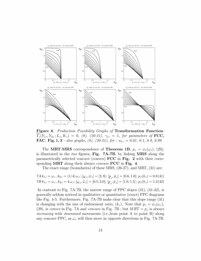
Figure 6. Production Possibility Graphs of Transformation Function:TJ(Y1J , Y2J ;LJ , KJ) = 0, (8), (20-21), γiJ = 1, for parameters of FCC,FAC, Fig. 1, 3 - also graphs, (8), (20-21), for : a1J = 0.01, 0.1, 0.9, 0.99.

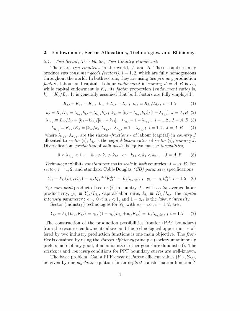
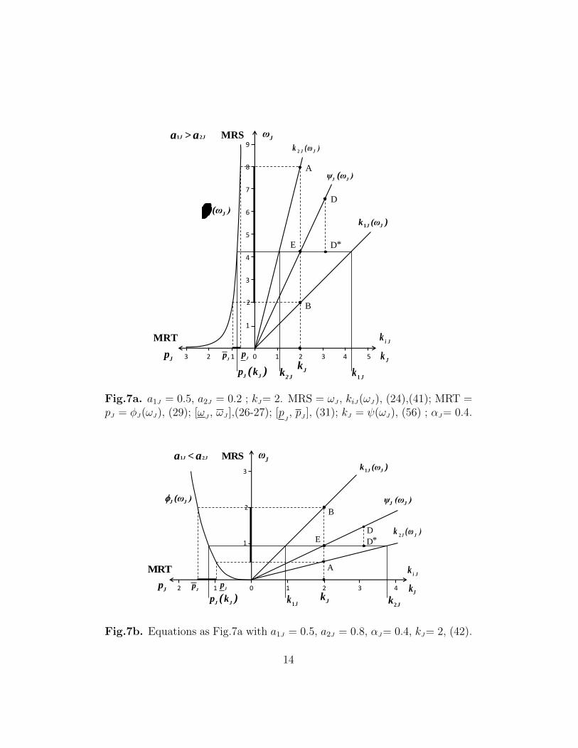
The MRT-MRS correspondence of Theorem 1B, pJ = φJ(ωJ), (29),is illustrated in the two figures, Fig. 7A-7B, by linking MRS along theparametrically selected concave (convex) FCC in Fig. 2 with their corre-sponding MRT along their always concave PCC in Fig. 4.

The exact range (boundaries) of these MRS, (26-27), and MRT, (31) are:

7Ak1J = ωJ , k2J = (1/4)ωJ ; [ωJ , ωJ ] = [2, 8]; [pJ, pJ ] = [0.6, 1.0]; pJ(kJ) = 0.8(41)

7B k1J = ωJ , k2J = 4ωJ ; [ωJ , ωJ ] = [0.5, 2.0]; [pJ, pJ ] = [1.0, 1.5] ; pJ(kJ) = 1.2(42)

In contrast to Fig. 7A-7B, the narrow range of PPC slopes (31), (41-42), isgenerally seldom noticed in qualitative or quantitative (exact) PPC diagramslike Fig. 4-5. Furthermore, Fig. 7A-7B make clear that this slope range (31)is changing with the size of endowment ratio, (kJ). Note that pJ = φJ(ωJ),(29), is convex in Fig. 7A and concave in Fig. 7B ; but MRT = pJ is alwaysincreasing with downward movements (i.e.,from point A to point B) alongany concave PPC, as ωJ will then move in opposite directions in Fig. 7A-7B.

13

5 4 3 2

9

8

7

6

4

3

2

1

5

1 1 3 2 0

Jω

2 J Jk (ω )

J Jψ ω )(

1J Jk (ω )

1 JkJ

k2 J

k

Jp

Jp

J Jp k( )

J J(ω )

MRT

Jp

i Jk

Jk

MRS

A

B

1 2J J>a a

E

D

*D

Fig.7a. a1J = 0.5, a2J = 0.2 ; kJ= 2. MRS = ωJ , kiJ(ωJ), (24),(41); MRT =pJ = φJ(ωJ), (29); [ωJ , ωJ ],(26-27); [p

J, pJ ], (31); kJ = ψ(ωJ), (56) ; αJ= 0.4.

1

2

3

3 2 1 0 1 2 4

1J Jk (ω )

2 J Jk (ω )

J Jψ (ω )

JωMRS

i Jk

Jk

MRT

Jp

J J(ω )

2Jk1 J

k Jk

B

A

Jp J

p

J Jp k( )

1 2J J<a a

ED

*D

Fig.7b. Equations as Fig.7a with a1J = 0.5, a2J = 0.8, αJ= 0.4, kJ= 2, (42).

14

4.1. Production Possibility Curves and the Elasticity of TransformationBesides our E (Y2J , Y1J), (22), it has been proposed to measure intrinsic

properties and the ”basic ’shape’ of the frontier of production possibilities bythe elasticity of transformation between products 1 and 2 - - The elasticity(τ) measures the responsiveness of the product ratio (”mix”) to changes inthe marginal rate of transformation”, Powell and Gruen (1968, p.315) :τ = E(Y2J/Y1J ,MRT ) = E(Y2J/Y1J , dY2J/dY1J).

The general analytic - algebraic expression for the substitution elasticityσ(k) of linear homogeneous production functions, Y = F (L,K) = Lf(k),Y/L = y = f(k) is the same as the transformation elasticity expression oftransformation functions for PPC curves, i.e., σ(k) for concave monotonicincreasing y = f(k) has the same formula as, τ(Y1J) for concave monotonicdecreasing, Y2J = TJ(Y1J) ≡ TJ(Y1J ;LJ , KJ) , 0 < Y1J < T−1J (Y2J = 0) :

Y2J = TJ(Y1J) ; T ′J = dY2J/dY1J < 0 , T ′′J = d 2Y2J/dY21J < 0 ; J = A,B (43)

Like, σ(k) > 0, the elasticity, τ(Y1J) < 0, can be stated, see Hicks (1932,pp.117-119, 242-245), cf. Arrow et al. (1961, p.230), Jensen (2017, p.65), as

E (Y2JY1J

,dY2JdY1J

) = E (TJ(Y1J)

Y1J, T ′J) ≡ τ(Y1J) = − [TJ − T ′J · Y1J ]T ′J

TJ · Y1J · T ′′J< 0 (44)

τ(Y1J) = τ : Y2J = TJ(Y1J) = γJ

[(1−bJ)−bJY

τ−1τ

1J

] ττ−1

, 0 < bJ < 1, γJ > 0 (45)

where τ(Y1J) = τ , is the special class of CET (Constant Elasticity of Trans-formation) curves that are obtained by integrating the second-order differen-tial equation, (44), and reparametrization/normalization of integration con-stants, cf. Arrow et al. (1961), Klump and Grandville (2000), Jensen (2017,p.76)- or (45) may be expressed more ’symmetrically’ as, C > 0, 0 < B <∞:

Yτ−1τ

2J = C−BYτ−1τ

1J ≥ 0 ;dY2JdY1J

= −B[Y2JY1J

] 1τ

; E (Y2J , Y1J) = −B[Y2JY1J

] 1+ττ

(46)

Y 22J +BY 2

1J = C, E (Y2J , Y1J) = −B ; Y 22J +Y 2

1J = C ; Y2J = [LJKJ−Y 21J ]

12 (47)

Unit elasticity, τ = −1, (47), gives positive orthants of ellipses and circles.CET curves (45-47) have horizontal/vertical tangents at axis intercepts, (46).

The PPC (19-22) do not have horizontal/vertical tangents at end (axis)points - and hence are not CET curves, but VET (Variable Elasticity ofTransformation) curves, i.e., cf, (44), (20) : τ(Y1J) = τ [h1 (λL1J

;LJ , KJ) ]will not turn out constant, but vary along PPC with λL1J

, similarly as theelasticity (22). Thus, PPC (frontier, envelope) curves derived with our twonon-joint product CD technologies (σ = 1) are VET transformation curves.

15

As a possible example of explicit transformation function, TJ(Y1J ;LJ , KJ),(production possibility frontier) graphs, Samuelson (1966, p. 34) examined

the positive orthant circle, (47) : Y2J = [LJKJ − Y 21J ]

12 - which satisfies

the required properties of concavity and homogeneity of first degree in thevariables (LJ , KJ , Y1J), and it had also twice continuously differentiability. Hehad verified that two countries, J = A,B, with common (identical) technologybehind transformation functions (PPF) as (47) would not have FPE (equalfactor prices by free trade). Concave PPF curves were essential elements inhis famous FPE theorem, Samuelson (1948, p.172), where two productionfunctions were assumed behind each country PPF curve, i.e, tacitly adopting(ruling out) non-joint production (sector outputs) in both countries.

So could (47) be obtained from two non-joint production functions ?and/or is joint production indeed behind the concave homogenous PPF (47)?There are several versions (characterizations) of the restrictions on a coun-try‘s transformation function (PPF) which are necessary conditions to satisfy,if the underlying technology is one of non-joint production. The simplestconditions relate to the rank of a singular, negative semi-definte Hessianmatrix of second-order partial derivatives of proposed (relevant) functionsTJ(Y1J ;LJ , KJ) to be: number of production factors - 1, i.e., here rank : 1 ;cf. Samuelson (1966, p.39), Burmeister & Turnovsky (1971, p.104).

To test for and identify uniquely two non-joint production functions be-hind, Y2J = TJ(Y1J ;LJ , KJ) = [LJKJ−Y 2

1J ]12 , (47), we are allowed to use the

same functional form of such non-joint functions F ∗iJ to test if they generatea transformation function T ∗J of the same functional form as TJ , (47) - whichevidently here suggests trying the CD functions, Samuelson (1966, p.38):

Y1J = F ∗1J = L121JK

121J , Y2J = F ∗2J = L

122JK

122J , K1J+K2J = KJ , L1J+L2J = LJ (48)

The maximal transformation function T ∗J then came from solving the con-strained maximum output problem (48) - this solution T ∗J is (33) in Ex. 1:

Y2J = T ∗J (Y1J ;LJ ,KJ) = [LJKJ ]12 − Y1J ; T ∗J (Y1J ;LJ ,KJ) < [LJKJ−Y 2

1J ]12 (49)

The Hessian matrix of T ∗J (49) has rank = 1 and is negative semi-definete, andhence it involves no joint production of its two outputs. The Hessian matrixof TJ (47) is singular, but has rank = 2 - so TJ (47) does intrinsically involvejoint production. TJ is everywhere larger than T ∗J , (49), and Samuelsoninterprets here TJ , e.g., as involving intermediate goods that can next be”cracked to make alternative amounts of good Y1J and Y2J as crude oil iscracked to variable proportions of gasoline and kerosene.”

16

Thus, apart from the ”Ricardo extension” of linear PPF, (33), (48-49),Samuelson (1966, p.35) indeed wished : ”I could write down an analyticexpression for TJ which comes definitely from a technology which involvesno joint production. But also, even though modern and older economistsspend most of their time in talking about the case where joint productionis not permitted, I do know an analytic expression for only one non-trivialcase, that in which one good uses but one the factors”. As far as we know theliterature, there is still not anywhere for the beloved 2-factor 2-good case givenany analytic expression for the PPF with non-joint production underlyingthe transformation function, Y2J = TJ(Y1J ;LJ , KJ). However, our reader hasseen such analytic and explicit TJ in Theorem 2, (34-36), that admittinglyeven with CD technology is an intricate nonlinear formula.

Incidentally, note that TFP parameters - γiJ - appear in many (all) termstogether with the outputs in (35). Evidently, if the intensity parameters arethe same, distinct γiJ are crucially important for a unique non-joint produc-tion behind T ∗J , i.e., γiJ = 1 or γiJ = γJ , are not admissible in (48-49), whennon-joint production is to be excluded - as it was by our distinct γiJ in (33).Burmeister & Turnovsky (1971, p.100) raise a non-joint problem with T ∗J :Y2J = T ∗J (Y1J ;LJ , KJ) = L1−aJ

J K aJJ − Y1J as PPF for an economy producing

Y1J and Y2J non-jointly, which here also require distinct γiJ as shown in (32).The two-good case, Samuelson (1966, p.35), with one sector (good) (Y1J)

only using one factor (e.g., Labor, L1J) has - with constant returns to scaletechnologies and CD - an analytic PPF of Y2J = TJ(Y1J ;LJ , KJ) simply as :

Y1J = γ1JL1J ; Y2J = γ2J(LJ − Y1J/γ1J)1−a2JKa2JJ ≡ TJ(Y1J ;LJ ,KJ) (50)

If two CD sectors (6) use specific capital and labor as a common factor, then

Y2J = γ2J

[LJ −

[Y1J/γ1J

Ka1J1J

] 11−a1J

]1−a2JKa2J

2J ≡ TJ(Y1J ;LJ , K1J , K2J) (51)

i.e., PPF is given by just inserting (using) a single constraint, L2J = LJ−L1J .The graphics of (51) is seen in standard texts, e.g., Caves et al (2002, p.105),Sodersten & Reed (1994, p.31). The procedure (51)to get an explicit PPFcan be extended to many goods using one common primary factor. Moreover,as shown by Kemp et al (1985, p.376), a similar procedure for a smooth PPF(51) can be extended to N goods and M primary factors, if one good (Y2) isproduced with a smooth production function (using all M primary factors),and if all other N-1 goods are produced with fixed-coefficient technologies.

17

The extreme simplicity of this result and its proof was obtained by notingthat if all coefficients of production are fixed for all goods (sectors) but one,no optimization - as neither in (51) - is needed to get an explicit PPF function.

In the special CET class (45-47) of Transformation functions, we had :

TJ(Y1J , Y2J ; LJ ,KJ) = GJ(Y1J , Y2J) − C = Y2J + TJ(Y1J)− C = 0 (52)

where C = (LJ , KJ) was only one (composite) endowment (input). As wesaw, (48-49), the PPF (52) assumed or had the possibility of joint production(outputs). The function GJ(Y1J , Y2J) can be extended to a joint - productioneconomy of many final goods, GJ(Y1J , Y2J , . ., YNJ) ; GJ is called a Factor Re-quirement Function, Diewert (1974, p.119), which gives the minimal amountof single input (composite, λKiJ = λLiJ ) C needed to produce the outputs.Besides CET, (46), GJ of one input-multiple outputs have functional formsnot to be pursued here. Instead, we must now return to the actual VETproperties of explicit two-factor transformation functions of non-joint outputsY2J = TJ(Y1J ;LJ , KJ) that Samuelson (1966) wished to see, viz. (34-36).

4.2. Variable Transformation Elasticities - Non-Joint Production Technology

18

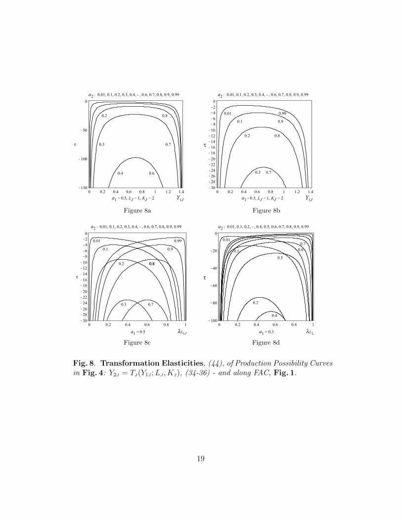
Figure 8a Figure 8b

Figure 8c Figure 8d

Fig. 8. Transformation Elasticities, (44), of Production Possibility Curvesin Fig. 4: Y2J = TJ(Y1J ;LJ , KJ), (34-36) - and along FAC, Fig. 1.

19

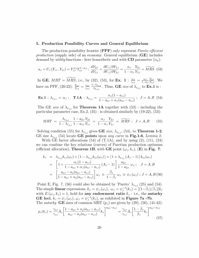
5. Production Possibility Curves and General Equilibrium

The production possibility frontier (PPF) only represent Pareto efficientproduction (supply side) of an economy. General equilibrium (GE) includesdemand by utility functions - here homothetic and with CD parameter (αJ):

uJ = UJ (Y1J , Y2J) = Y αJ1J Y

1−αJ2J ;

dY2JdY1J

=∂UJ/∂Y1J∂UJ/∂Y2J

=αJ

1− αJY2JY1J

= MRS (53)

In GE, MRT = MRS, i.e., by (32), (53), for Ex. 1 : γ2Jγ1J

= αJ1−αJ

Y2JY1J

. We

have on PPF, (20-22): Y2JY1J

= γ2Jγ1J

1−λL1J

λL1J

. Thus, GE size of λL1Jto Ex.1 is :

Ex.1 : λL1J= αJ ; T.1A : λL1J

=αJ(1− a1J)

1− a2J + αJ(a2J − a1J); J = A,B (54)

The GE size of λL1Jfor Theorem 1A together with (53) - including the

particular parameter case, Ex.2, (35) - is obtained similarly by (19-22), (53):

MRT =λL1J

1− λL1J

1− a2J1− a1J

Y2JY1J

=αJ

1− αJY2JY1J

= MRS ; J = A,B (55)

Solving condition (55) for λL1Jgives GE size, λL1J

, (54), to Theorem 1-2.GE size λL1J

(54) locate GE points upon any curve in Fig.1-6, Lemma 2.With GE factor allocations (54) of (T.1A), and by using (2), (11), (24)

we can combine the key relations (curves) of Paretian production optimum(efficient allocation), Theorem 1B, with GE point (ωJ , kJ), (E) in Fig. 7:

kJ = λL1Jk1J(ωJ) + [ 1− λL1J

k2J(ωJ) ] = [ 1 + λL1J(AJ − 1) ] k2J(ωJ)

=

[1 +

αJ(1− a1J)

1− a2J + αJ(a2J − a1J)(AJ − 1)

]a2J

1− a2JωJ ; J = A,B

=

[a2J − αj(a2J − a1J)

1− a2J + αj(a2J − a1J)

]ωJ ≡

βJ1− βJ

ωJ ≡ ψJ (ωJ) ; J = A,B (56)

Point E, Fig. 7, (56) could also be obtained by ’Pareto’ λL1J(25) and (54).

The simple linear expressions, kJ = ψJ (ωJ), ωJ = ψ−1J (kJ) = [(1−βJ)/βJ)]kJwith E (ωJ , kJ) = 1, hold for any endowment ratio kJ : i.e., the autarkyGE loci, kJ = ψJ (ωJ), ωJ = ψ−1J (kJ), as exhibited in Figure 7a -7b.The autarky GE sizes of common MRT (pJ) are given by (29), (56), (41-42):

pJ(kJ) =γ2J

γ1J

AJ

[1− a2J + αj(a2J − a1J)

a2J − αj(a2J − a1J)kJ

]a2J−a1J=γ2J

γ1J

AJ

[1− βJβJ

kJ

]a2J−a1J(57)

20

The GE size of λL1Jwas given in (54) - restated together with λK1J

(16) as,

λL1J=

1− a1J

(1− a2J)/αJ + a2J − a1J

; λK1J=

a1J

a2J/αJ + a1J − a2J

; J = A,B (58)

which are seen to be constant and endowment (kJ) invariant; moreover, alarger consumer preference (53) for good 1 (αJ) will by (58) imply largerfractions of both λL1J

and λK1J, whatever the sizes of a1J and a2J are.

The factor shares (relative remunerations, factor imputations) of laborand capital, δLJ , δKJ , in Pareto efficient production follow from (23) as :

δLJδKJ

=∂FiJ/∂LiJ∂FiJ/∂KiJ

· LJKJ

=MRS

KJ/LJ=

ωJkJ

=1− a2Ja2J

1

1 + (AJ − 1)λL1J

(59)

δLJ =1− a2J

1 + a2J (AJ − 1)λL1J

, δKJ = 1− δLJ ; J = A,B (60)

e.g. factor shares δLJ - for a given kJ - follow ωJ from A to B, in Fig. 7a-7b.The GE size of δLJ , δKJ , are obtained from (60), (58), and (11), and become:

δLJ = 1− a2J + αj(a2J − a1J) , δKJ = a2J − αj(a2J − a1J) = βJ ; J = A,B (61)

which are constant and endowment (kJ) invariant in CD GE economies.

5.1. Dual Money Cost Functions, Factor Prices and Commodity Prices

Standard dual minimal sector cost functions CiJ , and the unit costs ciJ ,of FiJ (6) are [wiJ , riJ are money factor prices of labor, capital ] in sector (i ):

CiJ(wiJ , riJ , YiJ) =1

γiJ

[wiJ

1− aiJ

]1−aiJ[ riJaiJ

]aiJYiJ ; PiJ = ciJ =

CiJYiJ

; i = 1, 2 (62)

Pareto efficiency comes now by free factor mobility and uniform factor prices,

MRS = ωJ = wJ/rJ ≡ wiJ/riJ , i = 1, 2 ; MRT = pJ ≡ P1J/P2J (63)

The relative commodity prices (unit costs), derived from (62-63), become :

pJ =P1J

P2J

=c1J (ωJ)

c2J (ωJ)=

γ2J

γ1J

· aa2J2J (1− a2J)

1−a2J

aa1J1J (1− a1J)1−a1J · ω

a2J−a1JJ ≡ pJ(ωJ) (64)

i.e., the relative prices, pJ(ωJ) ≡ γ2Jγ1J

AJ ωa2J−a1JJ ≡ φJ(ωJ), as MRT in (29),

and Fig. 7a - 7b. Also pJ(ωJ), (64), is endowment invariant; pJ like ωJ in

21

(64) may seem to range from zero to infinity ; but the relevant intervals forrelative factor prices ωJ and relative commodity prices pJ in (64) are restrictedby given endowment ratios kJ as described by (26-27), (31) of Theorem 1Bthat were never zero or infinity like the tangent slopes of CET curves (45-47).The sectoral capital-labor ratios kiJ(ωJ) belonging to (64) may be derived byapplying Shephard’s Lemma to (62), which will give kiJ(ωJ), (24) - that willalso again give the autarky GE loci, kJ = ψJ (ωJ), ωJ = ψ−1J (kJ), as in (56).The Walrasian GE factor endowment - factor price locus, k = Ψ(ω), has itsbackground in growth theory, cf. Uzawa (1961, p.43), Jensen (2003, p.64).

The panels of Figure 7a - 7b summarize the four-way connections be-tween goods prices, factor prices, sector factor ratios and endowment ratios- a diagram, which except for the GE locus, was introduced by Samuelson2

(1949, p.188), and is now familiar in texts at all levels. But their displayedgraphics of curves are only qualitative and often incoherent (especially, theleft panel cannot have straight lines). Fig. 7A-7B are rigorously extended toCES sector technologies in Jensen (2003, p.61); Kawano et al. (2017, p.992).

5.2. Pareto Efficient Allocations, Revenue Functions, General Equilibrium

The explicit Transformation Function, Y2J = TJ(Y1J ;LJ , KJ), or analytic

Production Possibility Frontier, TJ(Y1J , Y2J ; LJ , KJ) = 0, give a RevenueFunction, YJ = RJ (P1J , P2J , LJ , KJ), Feenstra (2004, p.6), Samuelson (1953-1954, p.10), (Maximum Value-Added = Gross National Product = YJ) :

YJ = RJ(P1J , P2J , LJ ,KJ) = maxY1J ,Y2J

{P1JY1J +P2JY2J}, s.t. TJ(Y1J , Y2J ;LJ ,KJ) = 0

(65)

with Y1J , Y2J in (65) being the explicit or the implicit function solutions

from: TJ(Y1J , Y2J ;LJ , KJ) = 0, in Theorems 1-2.

2He used, Li/Ki = 1/ki, on the right horizontal axis; hence in Fig. 7A-7B, the rays(24) would then be two rectangular hyperbolas: ωi = [(1−ai)/ai]/ki. It is more convenientwith the curves ωi(ki) always to originate from: (0, 0); it also applies to: k = Ψ(ω), (56).

22

With exogenous prices (P1J , P2J) and endowments (LJ , KJ), the maximizedmonetary value of outputs, YJ (65) is analytically obtained by (20-21), (30),

YJ ≡ P1JY1J + P2J Y1J ; YJ = wJLJ + rJKJ ; J = A,B (66)

= P1J LJ h1(λL1J(pJ ; kJ) ; kJ) + P2J LJ h2(λL1J

(pJ ; kJ) ; kJ) (67)

= P1J LJ γ1J λL1J(pJ ; kJ)

[ AJ kJ1 + (AJ − 1)λL1J

(pJ ; kJ)

]a1J +

P2J LJ γ2J [1− λL1J(pJ ; kJ) ]

[ kJ1 + (AJ − 1)λL1J

(pJ ; kJ)

]a2J (68)

≡ RJ (P1J , P2J , LJ ,KJ) ≡ P2J RJ (pJ , LJ ,KJ) ≡ P2J LJ RJ (pJ , kJ) (69)

i.e., RJ is a concave function (cone), (68), in the factor endowments (LJ , KJ),and a linear homogeneous convex function in (P1J , P2J).

Maximizing GNP, (65), the Pareto efficient economy (66-69) produceswith relative price, −pJ = −P1J/P2J = dY2J/dY1J , (19) - hence with (22):

E (Y2J , Y1J) = −P1JY1JP2JY2J

= − s1J1− s1J

= −1− a2J1− a1J

λL1J(pJ ; kJ)

1− λL1J(pJ ; kJ)

(70)

where, P1JY1J/P2JY2J = s1J/(1 − s1J), with s1J = P1JY1J/YJ as GNP finalexpenditure share of good 1, (65). Solving (70) for λL1J

(pJ ; kJ) gives, cf. (58),

λL1J(pJ ; kJ) =

1− a1J

[1− a2J ]/s1J + a2J − a1J

; s1J =[1− a1J ]λL1J

(pJ ; kJ)

1− a1J + [a1J − a2J ]λL1J(pJ ; kJ)

(71)

The MRT procedure (70-71) satisfies GE condition (54-55), if s1J = αj.GNP factor shares of labor, capital, δLJ , δKJ follow from (61) - with s1J :

δLJ = 1− a2J + (a2J − a1J)s1J , δKJ = a2J − (a2J − a1J)s1J ; J = A,B (72)

where the sectoral cost shares of labour and capital with (62-63) are :

εLiJ =wJ LiJCiJ

= 1− aiJ , εKiJ =rJ KiJ

CiJ= aiJ ; i = 1, 2 , J = A,B (73)

Later, we need another simple GNP expression involving δLJ , cf. (71-72) :

δLJ/s1J = (1− a2J)/s1J + a2J − a1J = (1− a1J)/λL1J(pJ ; kJ) ; J = A,B (74)

The explicit (parametric) Revenue Function (65-69) represents the dual(money cost, price) monetary version of the Pareto efficient allocations de-scribed by the analytic Transformation Functions in Theorem 1A-1B

23

and Figure 7a-7b - a unifying analytic framework for the Stolper-Samuelsonand Rybczynski theorems and their reciprocity (”symmetry”) relation.

E (MRT,MRS ) = E(pJ , ωJ) = E[P1J

P2J

,wJrJ

]= a2J − a1J (75)

By the standard elasticity rules, Allen (1938, pp.252), we get from (80) :

E(P1J , wJ) = a2J − a1J = −E(P1J , rJ) = E(P1J , 1/rJ) (76)

E(P2J , wJ) = a1J − a2J = −E(P2J , rJ) = E(P2J , 1/rJ) (77)

The inverse (reciprocals) of (76-77) give the Stolper-Samulson elasticities :

∂wJ∂P1J

P1J

wJ= ES(wJ , P1J) =

1

a2J − a1J

= ES(rJ , P2J) =∂rJ∂P2J

P2J

rJ(78)

∂wJ∂P2J

P2J

wJ= ES(wJ , P2J) =

1

a1J − a2J

= ES(rJ , P1J) =∂rJ∂P1J

P1J

rJ(79)

Dixit & Norman only inequalities forThey are larger than one and are positive or negative endowment invariantStolper comparative statics is vertical movements in Figure 7a-7b and

Rybszinki to horizontal

ER(Y1J , LJ) ≡ ∂Y1J∂LJ

LJY1J⇔ [

∂Y1J∂LJ

=∂wJ∂P1J

]⇔ ∂wJ∂P1J

P1J

wJ

wJP1J

LJY1J≡ ES(wJ , P1J)

δLJs1J

≡ ES(wJ , P1J)1− a1J

λL1J(pJ ; kJ)

≡ 1− a2J

(a2J − a1J)s1J+ 1 (80)

ER(Y2J , LJ) ≡ ES(wJ , P2J)1− a1J

λL1J(pJ ; kJ)

≡ 1− a1J

(a1J − a2J)s2J+ 1 (81)

ER(Y1J ,KJ) ≡ ES(rJ , P1J)1− a1J

λL1J(pJ ; kJ)

≡ a2J

(a1J − a2J)s1J+ 1 (82)

ER(Y2J ,KJ) ≡ ES(rJ , P2J)1− a1J

λL1J(pJ ; kJ)

≡ a1J

(a2J − a1J)s2J+ 1 (83)

The Stolper-Samuelson theorem established comparative static implica-tions of MRT- MRS correspondence : pJ= φJ(ωJ), (29), (64), Figure 7a-7b- showing conclusively that depending on technology parameters the real fac-tor reward (and factor share) (58) of one factor will fall (rise) with changesin MRT = pJ (commodity prices) - quantitatively expressed by, cf. (29)

24

Final CommentTheorem 1B supplemented the space coordinates representations of FCC/PCCin Lemma 1/Theorem 1 by using their ’tangential’ coordinates to carry thelink (interactions) between optimal changes of variables in factor and outputspace. Theorem 1B equations are suitable for generating comparative staticimplications and general equilibrium solutions of endowment variations (kJ).

By not only codifying past aspects of transformation functions, Paretoefficient allocations, extended with closed parametric form solutions, we lookforward to research generalized to other technologies (CES), with conjecturesto verify (correct) in micro, general equilibrium, trade and welfare economics.

25

6. References

Allen, R.G.D., 1938. Mathematical Analysis for Economists. Macmillan,London.

Arrow, Kenneth J., Chenery, Hollis B., Minhas, Bagicha S. and Solow,Robert M., 1961. Capital-Labor Substitution and Economic Efficiency, Re-view of Economics and Statistics , 43, 225-50.

Black, J., 1957. A Formal Proof of the Concavity of the ProductionPossibility Function, Economic Journal 67, 133-135.

Burmeister, Edwin and Turnovsky, Stephen J., (1971). The Degree ofJoint Production. International Economic Review, 12, 99-105.

Courant, R., 1937, 1988. Differential and Integral Calculus, Volume 1.Wiley Classics Library Edition, Interscience Publishers.

Edgeworth, Francis Y., 1881, 2003. Mathematical Psychics and FurtherPapers on Political Economy. P. Newman (ed.), Oxford University Press.

Deardorff, Alan V., 2006. Terms of Trade, Glossary of InternationalEconomics. World Scientific, Singapore.

Deardorff, A.V. and Stern, R.N., 1994. The Stolper-Samuelson Theorem:A Golden Jubilee. The University of Michigan Press, Ann Arbor.

Dixit, Avinash K. and Norman, Victor, 1980. Theory of InternationalTrade. Cambridge University Press.

Feenstra, Robert C., 2004. Advanced International Trade. PrincetonUniversity Press.

Haberler, Gottfried. 1936. The Theory of International Trade. W. Hodgeand Comp., London.

Hicks, John R., 1932, 1948. The Theory of Wages , Macmillan, London.Hsiao, Frank S.T. 1971. The Contract Curve and the Production Possi-

bility Curve. Journal of Political Economy, 79, 919–923.Jensen, Bjarne S., 2003. Walrasian General Equilibrium Allocations and

Dynamics in Two-Sector Growth Models. German Economic Review , 4, 53-87.

Jensen, Bjarne S., 2017. von Thunen : Capital, Production Functions,Marginal Productivity Wages and the Natural Wage. German EconomicReview , 18, 51-80.

Johnson, Harry G., 1966. Factor Market Distortions and the Shape ofthe Transformation Curve. Econometrica, 34, 686-698.

Kawano, Hidetaka, Ohta, Hiroshi, Jensen, Bjarne S. and Hwang, AmyR., 2017. Production, Distribution, and Trade: General Equilibrium with

26

One Single Cobb-Douglas Parameter. Modern Economy , 8, 970-993.Leontief, Wasily W., 1933. The Use of Indifference Curves in the Analysis

of Foreign Trade. Quarterly Journal of Economics , 47, 493-503.Klump, Rainer and de La Grandville, Olivier, 2000. Economic Growth

and the Elasticity of Substitution: Two Theorems and Some Suggestions.American Economic Review, 90, 282-291.

Lerner, A. P., 1933. Notes on Elasticity of Substitution - The Diagram-matical Representation. Review of Economic Studies, 1, 68-71.

Mass-Colell, Andreu, Whinston, Michael D., Green, Jerry R., 1995. Mi-croeconomic Theory, Oxford University Press.

Nicholson, Walter and Snyder, Christopher, 2012. Microeconomic The-ory, 11. ed., South-Western, Mason, OH, USA.

Rybczynski, T.M. 1955. Factor Endowments and Relative CommodityPrices. Economica, 22, 336-341.

Powell, Alan A. and Gruen, F.H.G., 1968. The Constant Elasticity ofTransformation Production Frontier and the Linear Supply System. Inter-national Economic Review, 9, 315-328.

Samuelson, Paul A., 1947, 1983. Foundations of Economic Analysis, En-larged Edition. Harvard University Press, Cambridge, Mass.

Samuelson, Paul A. (1948). International Trade and The Equalisation ofFactor Price. Economic Journal, 58, 163-184.

Samuelson, Paul A. (1949). International Factor Price Equalisation OnceAgain. Economic Journal, 59, 181–197.

Samuelson, Paul A. (1966). The Fundamental Singularity Theorem forNon-Joint Production. International Economic Review, 7, 34-41.

Samuelson, Paul A., 1972. Maximum Principles in Analytical Economics.American Economic Review , 62, 249-262.

Scarth, W.M. and R.D. Warne, R.D., 1973. The Elasticity of Substitutionand the Shape of the Transformation Curve. Economica, 40, 299–304.

Silberberg, Eugene, 1974. A Revision of Comparative Statics Methodo-logy in Economics. Journal of Economic Theory, 7, 159-172.

Silberberg, Eugene and Suen, Wing, 2001. The Structure of Economics,A Mathematical Analysis, 3. edition. Irwin McGraw-Hill, Boston.

Stolper, Wolfgang F. and Samuelson, Paul A., 1941. Protection and RealWages. Review of Economic Studies, 9, 58-73.

Suen, Wing, Silberberg, Eugene and Tseng, Paul, 2000. The LeChatelierPrinciple : The long and Short of It. Economic Theory, 16, 471-476.

27