Embed Size (px)
Citation preview
Distribution Category:Mathematics and Computer
Science (UC-405)
ANL--87-26-Vol.2
DE89 006399
ARGONNE NATIONAL LABORATORY9700 South Cass Avenue
Argonne, Illinois 60439-4801
PROCEEDINGS OF THE FOCUSED RESEARCH PROGRAM ONSPECTRAL THEORY AND BOUNDARY VALUE PROBLEMS
VOL. 2: SINGULAR DIFFERENTIAL EQUATIONS
,c c o
r. .. :'0 3 0 0c
0 - O 'a-v> 0
c E coEo '
p c
QCi1C uC C.
p O> * C '
C'. Q 0 e. $
0 A . C u
0 C2 C C 0 tiC..0~CF
:E _
Hans G. Kaper, Man Kam Kwong, and Anton Zettl, organizers
Gail W. Pieper, technical editor
Mathematics and Computer Science Division
September 1988
This work was supported in part by the Applied Mathematical Sciences subprogram of theOffice of Energy Research, U. S. Department of Energy, under Contract W-31-1((9-Eng-38.

A major purpose of the Techni-cal Information Center is to providethe broadest dissemination possi-ble of information contained inDOE's Research and DevelopmentReports to business, industry, theacademic community, and federal,state and local governments.
Although a small portion of thisreport is not reproducible, it isbeing made available to expeditethe availability of information on theresearch discussed herein.
Contents
Preface ....................................................................................................................................... viiList of Participants and Visitors .................................................................................................. ixSchedule of Talks ........................................................................................................................ xi
Asymptotics of an Eigcnvalue Problem Involving an Interior Singularity - F. V. AtkinsonAbstract ............................................................................................................................
1. Introduction ........................................................................................................... 12. Regularization Techniques......................................................................... ... 23. The First-Order System.............................................................................................34. Interface Conditions...................................................................................................45. The M odified Prufer Substitution..............................................................................66. The Main Result........................................................................................................77. A First Integration ..................................................................................................... 98. Proof of Theorem 1 ............................................................................................. 119. Proof of Theorem 2.................................................................................................13
10. The Case q(x) = -I/x..............................................................................................1411. The Cases q(x) = 11, C .............................................................................. 1612. Approximation of Potentials ................................................................................... 16Acknowledgments .......................................................................................................... 17References ...................................................................................................................... 17
Estimation of the Titchmarsh-Weyl Function m(A) in a Case with an Oscillating LeadingCoefficient - F. V. Atkinson
Abstract .......................................................................................................................... 191. Introduction ............................................................................................................. 192. The M ain kesult.................................................................................................. 223. A Preliminary Bound...............................................................................................234. A Scaled Riccati Equation.......................................................................................275. The Limiting Riccati Equation ................................................................................ 306. A Result of Everitt-Halvorsen Type........................................................................337. Bessel Functions - 1................................................................................................348. Bessel Examples - 2................................................................................................369. The Intermediate Case.............................................................................................38
References......................................................................................................................41
On the Order of Magnitude of Titchmarsh-Weyl Functions - F. V. AtkinsonAbstract .......................................................................................................................... 45
1. Introduction ............................................................................................................. 452. Lemmas on Riccati Equations ................................................................................. 473. The Case of a Dirac System....................................................................................494. Bounds for the Dirac Case ...................................................................................... 515. Discussion and an Example....................................................................................526. The Sturm-Liouville Case: A Preliminary Estimate ................................................ 537. The Sturm-Liouville Case: Two-sided Bounds ....................................................... 558. Sturm-Liouville Examples ....................................................................................... 579. A Special Example .................................................................................................. 5810. Asymptotics for Small A.........................................................................................62Acknowledgments .......................................................................................................... 63References ...................................................................................................................... 64
I, iii
Regularization of a Sturm-Liouville Problem with an Interior Singularity Using Quasi-Derivatives - F. V. Atkinson, W. N. Everitt, and A. Zettl
Abstract .......................................................................................................................... 671. Introduction ......................................................................................................... 672. Definition of the Operator S....................................................................................693. Regularization of the Singularity ............................................................................. 734. Numerical Results....................................................................................................755. The Interval (-o,oo).................................................................................................76
Acknowledgments .......................................................................................................... 77References ...................................................................................................................... 77
Asymptotics of the Titchmarsh-Weyl m-Coefficient for Nonintegrable Potentials - F. V. Atkin-son and C. T. Fulton
Abstract .......................................................................................................................... 791. Introduction ......................................................................................................... 792. Transformation to a Regular Sturm-Liouville Problem ........................................... 883. The Main Result......................................................................................................934. Proof of Theor m 2.................................................................................................955. Examples ................................................................................................................. 976. An Independent Check: q(x) = -&/x........................................................................99
References....................................................................................................................102
A Note on the Titchmarsh-Weyl m-Function - C. BennewitzAbstract ........................................................................................................................ 105
1. Introduction............................................................................................................1052. The Series .............................................................................................................. 1063. The m-function ...................................................................................................... 109
References .................................................................................................................... 111
Spectral Analysis of a Fourth-Order Singular Differential Operator - Hans G. Kaper andBernd Schultze
A bstract ....................................................................................................................... 1131. Introduction............................................................................................................1132. Definitions and Basic Properties............................................................................1143. Essential Spectrum.................................................................................................1154. Discrete Spectrum..................................................................................................1195. Conclusions ........................................................................................................... 122
References .................................................................................................................... 123
Singular Self-Adjoint Sturm-Liouville Problems, I: A Simple Approach to the Problem withSingular Endpoints - A. M. Krall and A. Zettl
Abstract ........................................................................................................................ 1251. Introduction............................................................................................................1252. Singular Boundary Conditions...............................................................................1273. Proofs and the Bridge to the Operator Theoretic Characterization ...................... 131
References .................................................................................................................... 137
Singular Self-Adjoint Sturm-Liouville Problems, II: Interior Singular Points - A. M. Krall andA. Zettl
Abstract ........................................................................................................................ 1391. Introduction............................................................................................................1392. Green's Formulas .................................................................................................. 1413. General Boundary Conditions................................................................................1434. Restrictions of LM, Self-Adjointness ..................................................................... 1445. Exam ples ............................................................................................................... 146
References .................................................................................................................... 148
iv
A Constructive Lemma for the Deficiency Index Problem - J. W. NeubergerAbstract ........................................................................................................................ 149
1. Introduction............................................................................... ...... 1492. Notation ................................................................................................................. 1493. Indication of Proof of Lemma...............................................................................1504. Applications...........................................................................................................1525. Computer Code......................................................................................................152
References .................................................................................................................... 152
Spectral Properties of Not Necessarily Self-Adjoint Linear Differential Operators - BerndSchultze
Abstract .................................................................................................................... 1531. Special Expressions ............................................................................................... 1542. Perturbations of Special Expressions................................................................ 1563. Results ................................................................................................................... 1574. The Casea> p . . . . . . . . .. . ... ... .. .. . . . . . . . . . . . . . . . . . . . . 161
Refer nces.. ............................................................ ............................................ 164
Analysis of the Asymptotic Behavior of the Linearized Stagnation Flow Equation of theKuramoto-Sivashinsky Type - E. Socolovsky and G. K. Leaf
Abstract ........................................................................................................................ 1671. Asymptotic Approximation Using Laplace Contour Integrals...............................168
1.1 Introduction .................................................................................................... 1681.2 Laplace Contour Solutions ............................................................................. 1681.3 Steepest Descent Method................................................................................1701.4 Asymptotic Approximation with Steepest Descent ........................................ 1731.5 Steepest Descent Paths ................................................................................... 1751.6 Fourth Contour and Solution..........................................................................1781.7 Summary ........................................................................................................ 181
2. Application of the WKB Method .......................................................................... 182References .................................................................................................................... 191
K'
Preface
This is the second volume of a series of reports containing the proceedings of theFocused Research Program on "Spectral Theory and Boundary Value Problems,"which was held at Argonne National Laboratory (luring the period 1986-1987. Theprogram was organized by the Mathematics and Computer Science (MCS) Division aspart of its activities in applied analysis. Members of the organizing committee were F.V. Atkinson, H. G. Kapcr (chairman), M. K. Kwong, A. M. Krall, and A. Zettl.
The objective of the program was to provide an opportunity for research and exchangeof views, problems, and ideas in three main areas of investigation: (I) the theory ofsingular Sturm-Liouville equations, (2) the asymptotic analysis of the Titchmarsh-Weylm()-coefficient, and (3) the qualitative theory of nonlinear differential equations. Theprogram had five full-time participants, who were joined by five more participants forperiods of several months. Twenty-four mathematicians from the United States,Canada, and Europe visited for shorter periods for seminars and technical discussions.These proceedings are the permanent record of the research stimulated by the year-longprogram.
The MCS Division generously supported the activities of the Focused Research Pro-gram. A grant for the visitors program was provided by the Argonne UniversitiesAssociation Trust Fund.
Following this preface is a list of all participants and visitors with their currentaffiliations and addresses. Also included is a schedule of the talks presented as part ofthe research program. We express our gratitude to our colleagues and especially tothose who contributed manuscripts to the proceedings.
Hans G. KaperMan Kam Kwong
Anton Zettl
' VII
Argonne National LaboratoryMathematics and Computer Science Division
1986-87 Focused Research Program"Spectral Theory and Boundary Value Problems"
Participants
Part-timeFull-time
F. V. AtkinsonDepartment of MathematicsUniversity of TorontoToronto M5S 1AI, OntarioCanadaOctober 1986 - July 1987
Hans G. KaperMathematics and Computer Science Div.Argonne National Laboratory9700 South Cass AvenueArgonne, IL 60439-4844September 1986 - September 1987
Allan M. KrallDepartment of MathematicsPennsylvania State University215 McAllister BuildingUniversity Park, PA 16802September 1986 - May 1987
Man Kam KwongMathematics and Computer Science DivisionArgonne National LaboratoryArgonne, IL 60439 4844September 1986 - September 1987
Anton ZettiDepartment of Mathematical SciencesNorthern Illinois UniversityDeKalb, IL 60115September 1986 - June 1987
W. AllegrettoDepartment of MathematicsUniversity of AlbertaEdmonton, Alberta T6G 2G ICanadaDates of visit: April 28-30, 1987
Paul B. BaleyNumerical Mathematics DivisionSandia National LaboratoriesAlbuquerque, NM 87185Dates of visit: April 20-24, 1987
Alfonso CastroDepartment of MathematicsNorth Texas State UniversityDenton, TX 76203-5116May - July 1987
C. Y. ChanDepartment of MathematicsUniversity of Southwestern LouisianaLafayette, LA 70504-1010May - July 1987
Charles T. FultonDepartment of Applied MathematicsFlorida Institute of TechnologyMelbourne, FL 32901April - June 1987
Marc GarbeyDepartment of MathematicsU. de ValenciennesLe Mont Houy59326 ValenciennesFranceJune - July 1987
Eduardo SocolovskyDepartment of MathematicsUnivenity of PittsburghPittsburgh, PA 15260June - September 1987
Visitors
Chr. BennewitzDepartment of MathematicsUniversity of UppsalaSwedenDates of visit: March 17-31, 1987
H. BenzingerDepartment of MathematicsUniversity of Illinois273 Altgeld HallUrbana, IL 61801Dates of visit: March 16-17, 1987
,
R. C. BrownMathematics DepartmentUniversity of AlabamaTuscaoosa, AL 35487-1416Dates of visit: April 13-18, 1987
S. ChenDepartment of MathematicsShandong UniversityJinan, ShandongPeople's Republic of ChinaDates of visit: March 17-20, 1987
P. Concus50A-2129Lawrence Berkeley LaboratoryBerkeley, CA 94720Dates of visit: January 30-31, 1987
L. ErbeDepartment of MathematicsUniversity of AlbertaEdmonton, Alberta T6G 2G 1CanadaDates of visit: April 27-30, 1987
W. N. EverttDepartment of MathematicsThe University of BirminghamP. O. Box 363Birmingham B15 2TTUnited KingdomDates of visit: April 16-30, 1987
J. GoldsteinDepartment of MathematicsTulan' UniversityNew Orleans, LA 70118Dates of visit: May 13-14, 1987
G. HalvorsenInstitute for Energy TechnologyDepartment KRS, Box 402007 KjellerNorwayDates of visit: May 18-26, 1987
B. J. HarrisDept. of Mathematical SciencesNorthern Illinois UniversityDeKalb, IL 60115-2888Dates of visit: June-August, 1987
D. HintonDepartment o MathematicsUniversity of TennesseeKnoxville, TN 37996-1300Dates of visit: April 13-18, 1987
V. JurdJevkUniversity of TorontoToronto, Ontario MSS 1A1CanadaDate of visit: July 30, 1987
A. B. MingarellDepartment of MathematicsUniversity of Ottawa585 King EdwardOttawa KIN 6N5CanadaDates of visit: 3/1-7, 4/27-30, 5/22-23, 1987
J. NeubergerDepartment of MathematicsNorth Texas State UniversityP. O. Box 5116Denton, TX 76203-5116Dates of visit: April 1-4, 1987
S. PruessMathematics DepartmentColorado School of MinesGolden, CO 80401Dates of visit: June 15-19, 1987
T. ReadDepartment of MathematicsWestern Washington UniversityBellingham, Washington 98225Dates of visit: April 13-18, 1987
J. RidenhourDepartment of MathematicsUtah State UniversityLogan, UT 84322Dates of visit: May 13-20, 1987
Bernd SchultzeUniversitaet Gesmathochschule EssenFachbereich 6, MathematikPostfach 103 7644300 Essen 1West GermanyDates of visit: May 31-June 8, 1987
G. SellInst. for Mathematics and Its ApplicationsUniversity of Minnesota206 Church StreetMinneapolis, MN 55455Date of visit: April 23, 1987
J. SerrinDepartment of MathematicsUniversity of Minnesota206 Church StreetMinneapolis, MN 55455Date of visit: June 18, 1987
J. K. ShawDepartment of MathematicsVirginia Polytechnic Institute
and State UniversityBlacksburg, VA 24061Dates of visit: April 13-18, 1987
x
Argonne Natie'?'i LaboratoryMathematics and Computer Science Division
1986-87 Focused Research Program"Spectral Theory and Boundary Value Problems"
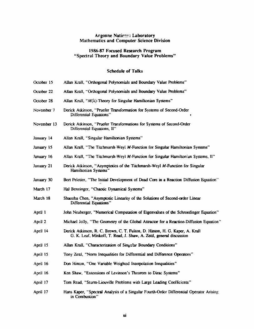
Schedule of Talks
October 15
October 22
October 28
November 7
November 13
January 14
January 15
January 16
January 21
January 30
March 17
March 18
April 1
April 2
April 14
April 15
April 15
April 16
April 16
April 17
April 17
Allan Krall, "Orthogonal Polynomials and Boundary Value Problems"
Allan Krall, "Orthogonal Polynomials and Boundary Value Problems"
Allan Krall, "M(X)-Theory for Singular Hamiltonian Systems"
Derick Atkinson, "Pruefer Transformation for Systems of Second-OrderDifferential Equations" "
Derick Atkinson, "Pruefer Transformations for Systems of Second-OrderDifferential Equations, II"
Allan Krall, "Singular Hamiltonian Systems"
Allan Krall, "The Titchmarsh-Weyl M-Function for Singular Hamiltonian Systems"
Allan Krall, "The Titchmarsh-Weyl M-Function for Singular Hamilton in Systems, II"
Derick Atkinson, "Asymptotics of the Titchmarsh-Weyl M-Function for SingularHamiltonian Systems"
Bert Peletier, "The Initial Development of Dead Core in a Reaction Diffusion Equation"
Hal Benzinger, "Chaotic Dynamical Systems"
Shaozhu Chen, "Asymptotic Linearity of the Solutions of Second-order LinearDifferential Equations"
John Neuberger, "Numerical Computation of Eigenvalues of the Schroedinger Equation"
Michael Jolly, "The Geometry of the Global Attractor for a Reaction-Diffusion Equation"
Derick Atkinson, R. C. Brown, C. T. Fulton, D. Hinton, H. G. Kaper, A. KrallG. K. Leaf, Minkoff, T. Read, J. Shaw, A. ZettI, general discussion
Allan Krall, "Characterization of Singular Boundary Conditions"
Tony Zettl, "Norm Inequalities for Differential and Difference Operators"
Don Hinton, "One Variable Weighted Interpolation Inequalities"
Ken Shaw, "Extensions of Levinson's Theorem to Dirac Systems"
Tom Read, "Sturm-Liouville Problems with Large Leading Coefficients"
Hans Kaper, "Spectral Analysis of a Singular Fourth-Order Differential Operator Arisingin Combustion"
xi
April 20 Paul Bailey, "Computation of Eigenvalues and Eigenfunctions of Sturm-Liouvillc Equationsusing SLIEICN"
April 21 Paul Bailey, "Computation of Eigenvalues and Eigenfunctions of Sturm-1 iouvil!c Equation;using SLEIGN, 11"
April 22 Norrie Everitt, "The Laplace Tidal Wave Equation"
April 23 George Sell, "The Principle of Spatial Averaging and Inertial Manifolds"
April 23 Paul Bailey, "Computation of Eigenvalues and Eigenfunctions of Sturm-Liouville Equationsusing SLEIGN, III"
April 28 Lynn Erbe, "Oscillation Theory for Systems of Second-Order Differential Equations"
April 29 Walter Allegretto, "Spectral Analysis of Second-Order Boundary Problems withIndefinite Weight Functions"
April 30 Charles Fulton, "Asymptotics of m(X) for Singular Potentials"
May 14 Jerry Goldstein, "Recent Developments in Thomas-Fermi Theory"
May 15 Charles Fulton, "Singular Hamiltonian Systems"
May 18 Jerry Ridenhour, "Zeros of Solutions of n-th Order Differential Equations"
May 20 Charles Fulton, "The Bessel-squared Operator in the lim-2, lim-3, and lim-4 Cases"
May 21 Gotskalk Halvorsen, "Oscillation Results for Second-Order Equations"
May 22 Derick Atkinson, "Estimation of m(X) in a Case with an Oscillating Leading Coefficient"
May 27 Hans Kaper, "A Non-oscillation Theorem for an Emden-Fowler Equation"
June 1 C. Y. Chan, "A Generalization of the Thomas-Fermi Equation"
June 3 Bernd Schultze, "Spectral Properties of Nonselfadjoint Differential Operators"
June 5 Alfonso Castro, "Superlinear Boundary Value Problems"
June 9 Man Kam Kwong, "Concavity of Solutions of Certain Emden-Fowler Equations"
June 15 Charles Fulton, "Convergence of Spectral Functions"
June 16 Bernie Matkowsky, "Introduction to Bifurcation Theory"
June 18 James Serrin, "Asymptotics of the Emden-Fowler Equation"
June 19 Steve Pruess, "SPDNSF: A Code to Compute the SPectral DeNSity Function"
June 25 Bernie Matkowsky, "Stability Analysis and Bifurcation Theory"
July 17 Marc Garbey, "A Quasilinear Prabolic-hyperbolic Singular Perturbation Problem"
July 30 Val Jurdjevic, "Differential Equations of Control Theory"
July 31 Bernie Harris, "Asymptotics of the Titchmarsh-Weyi m(X)-coefficient"
xii
ASYMPTOTICS OF AN EIGENVALUE PROBLEMINVOLVING AN INTERIOR SINGULARITY
F. V. Atkinson*Department of Mathematics
University of TorontoToronto M5S lAl, Ontario
Canada
Abstract
A regularization method is presented for obtaining asymptotic estimates ofeigenvalues of Sturm-Liouville problems with non-integrable potentials.
1. Introduction
For some time there has been interest in spectral problems for equations such as
-y"+Cx-y= ky, 0<x<-b, (1.1)
in the situation when the "singular potential" Cx-k is not integrable at the origin. A recent
paper [Atkinson and Fulton 19841 was devoted to the asymptotics of eigenvalues for a class of
such equations, including (1.1) in the range 1 S k < 2 as special cases; a sequel [Atkinson and
Fulton 1987] will examine the asymptotic; of the Titchmarsh-Weyl function in such situations.
More recently still, attention has been given to certain similar equations in which the singular-
ity occurs in the interior of the interval rather than at an endpoint. A case in point is given by
-y"-y/x=Xky, a x b, wherea<O<b. (1.2)
The aim of this paper is to use a modification of the techniques of [Atkinson and Fulton 1984]
to develop the asymptotics of eigenvalues of similar equations to (1.2), usually with Dirichlet
boundary conditions.
The functional analysis underlying (1.2) has been brought out in recent papers by Everitt,
Gunson, and Zettl [1987], Everitt and Zettl [1986,1987], Gunson [1987], and Zettl [1968] in
connection with a theory of spectral resolutions in direct sum spaces with interface conditions.
A quite distinct approach to (1.2) is given by a perturbation technique, in which the singular
potential - l/x is replaced by an integrable and indeed smooth approximation, such as
- x/(x2 + E2), (1.3)
for small e > 0; here we refer again to the work of the above authors.
Senior Mathematician Emeritus at the Mathematics and Computer Science Division, Argonne National La-boratory, 10/1/86 to 7/17/87.
1
Yet another device is to replace - 1/x by a complex approximation
- 1/(x + iE), (1.4)
again for small e > 0; here the approximating potential is again smooth, but no longer real-
valued, so that the spectrum may cease to be real. The use of this latter method in a paper by
Boyd [1981] has been seminal in this connection. Since our approach here is distinct from the
above three, we must refer to the cited papers for further discussion of these methods.
Sections 2 to 5 of this paper are devoted to transforming the problem to a regular form,
and to general discussion. The estimations of eigenvalues that form the main results are given
in Section 6, for a general class of potentials, with proofs in Sections 7 to 9. The example
(1.2) in the special case a = -1, b = 1 is discussed in Section 10, other examples being noted
in the following section. Finally, in Section 12, we indicate how approximation procedures
such as the use of (1.3) can be considered from the present point of view.
2. Regularization Techniques
We shall be concerned with an equation
- y" + g(x)y = Xy , x E [a,b] \(0} ,-x>< a 50< b <oo , (2.1)
where q is real and in L[a,0) + L(0,b], but may not be integrable rear x = 0. The case
a = 0, b > 0 was considered in [Atkinson and Fulton 1984] and, while formally covered here
(as is the ordinary nonsingular case), is not our main topic.
The procedure adopted in [Atkinson and Fulton 19841 for the latter one-sided problem
over (0,b] was to make a change of dependent variable
z = y/u (2.2)
for some positive and suitably smooth u, to obtain a new equation
- (u2 z')' + q*z = Xu2z , (2.3)
also of Sturm-Liouville type; here
q* = u(qu-u") . (2.4)
In the cases of interest, the coefficient u2 of z' in (2.3) is continuous and has a positive lower
bound, and so meets the generally accepted requirements for the "regular" case in Sturm-
Liouville theory. The singularity of q in (2.1) at x = 0 may still manifest itself in (2.3) in the
failure of u(x) to be continuously differentiable at x = 0; however, with the advent of "quasi-
derivatives", this failure need not exclude (2.4) from the regular category.
It is, of course, still necessary to consider whether the new "potential" q* was integrable,
unlike the old one. In [Atkinson and Fulton 1984], the basic idea was to choose u to be a
2
solution of (2.1) with X = 0 such that u(x) -+ 1 as x -4+0, provided of course that such a
solution exists; this makes q* = 0. In view of the possibility that such a solution might notremain positive over the whole interval (0,b], the choice 3f u could be modified over a sub-
interval [b'b]; we refer to [Atkinson and Fulton 1984, p. 55] for discussion and details.
From a theoretical standpoint, regularization provides a basis for extending the standard
results of Stu',mian theory to equations with an interior singularity, in particular the reality and
discreteness of the spectrum, together with oscillation and expansion theorems. Here the focus
will be on regularization as a route to workable asymptotics, and even numerical estimates.
The functions used for the regularization will be specified explicitly, rather than as solutions of
a differential equation.
We shall "regularize" an associated first-order Prifer differential equation rather than a
Sturm-Liouville type equation (2.3).
3. The First-Order System
For some real differentiable functionf on [a,0) u (0,] to be specified, we define
YI= YY2 = y' + yf, (3.1)
where y is a solution of (2.1). We then find that y,y2 satisfy the first-order system
= -fy + y2 (3.2)
Y2'Y=i(f' +q-f 2 -A)+fy 2 . (3.3)
For "regularity" we need that
fJE L(a,b) , (3.4)
f' + q -f 2 E L(ab) . (3.5)
We can then see (3.2)-(3.3) as a unified system over the whole interval [ab].
Various transformations are possible. We can of course trace our steps from (3.1)-(3.3)
to the original differential equation over the punctured interval with singularity. However, we
can also derive a regular Sturm-Liouville problem over the whole interval, subject to (3.4)-
(3.5). We define
F(x) = exp -ofJt)dt , Y(x) = y, (x)/F(x) , (3.6)
and then find that Y satisfies the non-singular Sturm-Liouville equation
-(F 2 Y')'+F2 (f''+q-f2)Y=XF2Y. (3.7)
3
The system can also be put in "canonical" or "Hariltonian" or again accommodated within
the general theory of regular quasi-differential expressions; a similar construction with the latter
interpretation has in fact been given in recent work of Everitt and Zettl [1987].
While these transformations are important in establishing the theoretical background, we
shall in fact work directly from (3.1)-(3.3).
We can ensure (3.4)-(3.5) in a simple, though slightly restrictive way, by defining f so
that
f -q , x E [ab]\{0) (3.8)
and postulating that
f 2 E L(ab) . (3.9)
As it happens, the asymptotic calculations will require that
f 3 e L(ab) . (3.10)
This will be applicable in particular in the cases
q(x)=Clxrk, 1<_k<4/3. (3.11)
We remark that the above constructions can be carried through in simpler situations such
as
(i) the case when the singularity occurs at an endpoint,
(ii) the case when the potential q is integrable at the singularity, and, of course,
(iii) the case when q is smooth in [a,b].
Thus our estimates can be seen as extensions of those for the regular case.
4. Interface Conditions
The interpretation of (3.1)-(3.3) as a single system over the whole interval over [a,b]
requires, of course, that y1,y2 should be continuous at x = 0. In the case of y, this means for
(2.1) that y is continuous, that is to say,
y(-0) = y(+0) , (4.1)
a natural (though not inevitable) requirement. The continuity of y2 means that
lim (y'(x) + y(x)f(x)) = lim (y'(x) + y(x)ffx)). (4.2)
Here it should be mentioned that the choice off to satisfy (3.8) involves the choice of two con-
stants of integration, one for each of [a,0), (0,b]. This choice must be expected to affect the
estimates for eigenvalues, though only in lower order terms.
4
We examine the second interface condition (4.2) in the case of main interest, (1.2) when
q(x) = -1/x . (4.3)
We take first the simple choice
ftx)=logIxI, a5x<0, O<x5b. (4.4)
Equivalently to (4.2), we have for small x * 0 that
y'(x) + y(x)loglx = y2(0) + o(1) , (4.5)
and here y(x) = y(O) + o(1). Hence
y'(x) = - y(0)logxl + o(loglxl) , (4.6)
and so
y(x) = y(O) + O(xloglxl) , (4.7)
whence
y'(x) + y(x)loglx = y'(x) + y(0)loglxil + o(1) . (4.8)
It then follows that the second interface condition (4.2) admits the interpretation
y'(E) - y'(-e) - 0 (4.9)
as E -+ +0. Except when y(O) = 0, both y'(e),y'(-e) will be unbounded, in view of (4.6).
A similar discussion has been given by Everitt and Zettl [19871.
More generally, we could have chosen
ftx)=loglx+C1 , a5x<0, ffx)=loglxl+C2 , O<x5b (4.10)
for any constants C1,C2. In this case (4.9) must be replaced by
y'(E) - y'(-E) + (C2 - C1)y(0) -+ 0 (4.11)
as E -+ +0.
In the case
q(x) = 1/IxI , (4.12)
we could take
fx) = - sgn x logLxid, (4.13)
which would lead to, in place of (4.9),
y'(E)-- y'(-E) - 2y(0)log E -+ 0 (4.14)
as E -+0.
5
The argument leading to (4.9) as a replacement for (4.2) extends to the situation that q(x)
is an odd function and f(x) an even function, with the property that
f(x)I f Idt -+0 (4.15)
as x -+ 0.
5. The Modified Prufer Substitution
We work directly from the system (3.2-3), with the choice (3.8) for f, rather than from
the regularized Sturm-Liouville equation (3.7); we recall that implicit in the choice of f lies, in
the singular case, a choice of two constants of integration. The system then takes the form
Y'= -fy + y2 , (5.1)
y2' = - (f2+ X)yi +fy2 (5.2)
For any nontrivial solution and any k > 0, we can define a function 4(x), to within additive
multiples of it, by
tan$ = kYI/y2 (5.3)
so that zeros of yi (or y) correspond to roots of $= 0 (mod. n). The differential equation
satisfied by $ is found to be
$' = k cos 2 $ + (1/k)(f 2+X)sin 2 $ -f sin 2n. (5.4)
This shows that $ is increasing as a function of x when it is a multiple of it, and also that it is
nondecreasing as a function of A for fixed x. Thus eigenvalues AX, n = 0,1,..., of the Dirichet
problem over (a,b) will be characterized by
$(a,X,) = 0 , 4$(b,,.) = (n+1)ni. (5.5)
For asymptotic purposes, and positive X, we take k = A in the above, and define
0 = 0(x,) according to
tanG = XAy/y2 , (5.6)
except at zeros of y2. A similar, though distinct, substitution was used in [Atkinson and Fulton
1984, p. 56]. We find, as the differential equation for 0,
0' = X" -f sin 20 + X- f 2 sin20 . (5.7)
The positive eigenvalues of the Dirichlet problem, for example, will be characterized by (5.5),
applied to 0(x,), that is to say,
0(a,XA) = 0 , 0(b,A,) = (n+1)n. (5.8)
6
In the case of the Neumann problem, the determining equation for positive eigenvalues
will be
0(a,X.) = ir/2 , 0(b,X.) = n(n + 1/2) . (5.8)
6. The Main Result
It follows easily from (5.8) and (3.9)-(3.10) that large positive eigenvalues of either the
Dirichlet or the Neumann problems over (a,b) will satisfy
= (n+1)n/(b-a) + 0(); (6.1)
this of course leads to an error 0(n) in the estimate of X,,. Here we find a two-stage improve-
ment, leading first to an error 0(n-1) in the estimate of A,, and the second to an error o(n ),the latter subject to a mild additional hypothesis. These lead to errors 0(1), o(1), respectively,
in the estimates for A,,.
We first collect our hypotheses, which are as follows:
(i) q is real and in L(a,0) + L(0,b) (i.e., the restrictions of q to the subintervals (a,0), (0,b) lie
in the respective L-spaces)
(ii) f is real,
f' = q (6.2)
a.e. in (a,0) u (0,b), and
f 3 E L(a,b) (6.3)
(iii) as x -* 0 we have
x(x) -+ 0 , (6.4)
(iv) we have
Iq(x)I {Jf(t)ldt + ff2(t)dt} E L(a,b) . (6.5)
We remark that it follows from (6.3) that
'ff2 E L(a,b) . (6.6)
In the case
q = Cx-k, (6.7)
the above conditions are satisfied i;
7
0 < k < 4/3.
As another type of example we cite
q(x) = x-2sinx-2 . (6.9)
Higher approximations to eigenvalues commonly involve a sort of Fourier coefficient of
the "potential". In our case we need to introduce, for A.> 0, the functions
h1() = Jq(x) sin 2xX Adx , (6.10)
b
h2() = Jq(x)(l - cos 2xX)ix. (6.11)
The above conditions, with (6.4) in particular, ensure that these integrals exist. In the case
q(x) = Clx they are known special functions, essentially sine and cosine integrals.
We formulate the basic result in terms of the change of the Prufer angle 0(x) = 0(x,1)
over (a,b) for large A.> 0. This can subsequently be translated into the behavior of eigen-
values in various circumstances.
THEOREM 1. As A -+ oo, we have
0(b) - 0(a) - (b-a)kA = - '7~(t(x){sin20(x) - sin20(0))] (6.12)
- (1/2)1-{sin 20(0)h 1(A) + cos 20(0)h 2(A)} + 0(1-).
For an improved error-bound, we need hypotheses involving integrals similar to those on
the right of (6.10)-(6.11). We define
p(.) = suplfq(t) sin 2tAkdtI + suplJoq(t)(1 - cos 2x")dt| , (6.13)
with "sup" over (a,b). We introduce for large 7L> 0 the interval
J(X) = (a,b)\(-A ), (6.14)
and require that, as A -+ oo,
p(L))Iqldt = o(0 A) ,(6.15)
191(1 + V)dt = o(') . (6.16)
For example, in the case (6.7) with k = 1, we have (cf. (10.6), (11.4))
p(X) = 0(logX)
for large 7, and so (6.15) holds, as does (6.16). If k > I we have
S
(6.8)
p() = 0(X(k-Y2) ,
and the left of (6.15) is 0(k~1), so that (6.15) holds when k < 3/2, as does (6.16).
We have then the following theorem.
THEOREM 2. With the additional hypotheses (6.15)-(6.16), we have that (6.12) holds, with the
error term replaced by o(G47).
We discuss briefly the application of these results to the estimation of eigenvalues. This
may be a two-stage process. In the first stage 0(a), 0(b) are equated to specific values, typi-
cally specified multiples of it, and (6.12) or its analog with a reduced error term is used as an
approximate equation to determine X. Here one notes that the right-hand sides involve the
unspecified quantity 0(0), but only in lower order terms, so that X is still determined to a cer-
tain degree of accuracy. In the second stage we apply (6.12) or a weaker result, over the inter-
val (a,0) with the value of X obtained from the first stage, to get an approximate value for 0(0),
namely, 0(a) - aX', which can then be inserted in the lower order terms in (6.12) when taken
over (a,b). We carry out this "bootstrap" process in some specific cases in Section 10.
7. A First Integration
We now investigate (5.7) as X -+ oo, and need two lemmas.
LEMMA I. Let x1 , x2 satisfy
a 5 x1 < x2 5 b , (7.1)
and also
x2 -x 1 5 SX- (7.2)
for some fixed 5 > 0. Then
0(x 2) - 0(x 1) = (x2 - x1)X" + o(l). (7.3)
Integration of (5.7) yields
10(x2) - 0(x1) - (X-i~u 5 I f sin 20 dxl + ~"Jf 2 dx . (7.4)
Here the first term on the right is o(l) since f E L(a,b) and since x2 - x1 = o(1). The last term
on the right is o(l) since f e L2(a,b) and since )~ = o(l). This proves Lemma 1.
LEMMA 2. The result of Lemma I holds without the hypothesis (7.2).
We write p. = c/(2X 1h). By (7.4), we need to show that
9
Jfsin 20dx=o(1). (7.5)
By Lemma 1, it will be sufficient to show this for the case that
x+ps b , x2 - x 1 I. (7.6)
We write
1= L fsin 20 dx, I' = f sin 20 dx.
Since f E L(a,b) and .t = o(l), we have
I - 1' = o(1) . (7.7)
We plan to prove that
1+1' = o(1), (7.8)
so that (7.7)-(7.8) will prove L.:mma 2.
Now
I + I' = o(1) + J {fix) sin 20(x) +f(x+ ) sin 20(x+))}dx
= o(l) + J f(x){sin 20(x) + sin 20(x+))dx (7.9)
x
+ Jsin 20(x+ ){(f(x+ ) - fx))}dx.
Here the last term is o(1) since
J ix+ ) -fx)ldx = 0(1)
this being so since f e L(a,b). Also
sin 20(x+ ) + sin 20(x) = 2 sin (0(x+s) + 0(x)) cos (0(x+ ) - 0(x))
and here 0(x+ ) - 0(x) = c/2 + o(l), by Lemma 1. This shows that the remaining term on the
right of (7.9) is also o(l). This proves (7.8), and so Lemma 2.
We need later the properties stated in Lemma 3.
LEMMA 3. As A -+ oo,
J2cos 20 dx = o(1) , ff2cos 40dx = o(l) . (7.10)
These are proved in the same way as (7.5).
As a preliminary result on eigenvalues we have the following.
LEMMA 4. For large n the eigenvalue A,, of the Dirichlet problem given by (2.1), the
10
boundary conditions
y(a) = y(b) =0, (7.11)
and the interface conditions of Section 4 satisfy
(n+1)it = (b-a)CA + o(l) . (7.12)
This follows from Lemma 2. In this paper the eigenvalues are denoted
(-oo<) o<X1 < < --. (7.13)
8. Proof of Theorem 1
We now improve the result of Lemma 2, with a view to reducing the error to O(X~A).
We write the result of integrating (5.7) in the form
0(b) - 0(a) - (b-a)A"= -11 + 12, (8.1)
whereb
11=J fsin 20 dx, (8.2)
b
'2 ;=A hJaf2 sin20 dx . (8.3)
The term '2 is easily dealt with. Using (7.10) we haveb
'2 = (1/2)A_- f2 dx + o(k7'n). (8.4)
We pass to the term I. We write (5.7) in the form
1 = 0'x-' + ?- 'f sin 20 - ?-If 2 sin20 (8.5)
and so, inserting this factor under the integral sign, get
11=111 + 12 -113, (8.6)
where
111= ?- bf0'sin20dx, (8.7)
b
'12 = X_"faf2sin2 0 dx , (8.8)
b
li3 = -J f 3sin2 0 sin 20 dx. (8.9)
Here, by (7.10),
'12 = (1/2)X-Af 2dx + o('4) , (8.10)
and
11
X13 =0(-).
Hence, using (8.4) and (8.10), we get
0(b) - 0(a) - (f-a)l/J = - 1I + o07w ). (8.12)
To estimate the term 11, we integrate by parts. If f is continuous at 0, and so if
q e L(a,b), this takes the simple formb
111 = A-'f sin20]J + ~'jq sin2 0 dx , (8.13)
since f' = -q. In the general singular case this will not be admissible, and we replace (8.13)
by
111 = ?~"(f(sin 2 0(x) - sin2 0(0))]a + X~1f q{sin20(x) - sin20(0))dx (8.14)
=f1l1 + 1112
Before proceeding, we remark that in this partial integration we have assumed that the
integrated term fsin20(x) - sin20(0)) is continuous at 0. In fact, it tends to 0 as x - 0. To
verify this, we note that, by (5.7),
10(x) - 0(0)1 5 Ikuxl + Ifldtl + 1AJff2dtI , (8.15)
so that
If(sin 20(x) - sin2 0(0)I 5 lxf4(x)I + fix)4f dtI + X-"Ifx)Jf2dtI . (8.16)
The hypotheses of Section 5 ensure that the terms on the right all tend to 0 as x -4 0.
The term 1111 already appears in the main result of Theorem 1 and needs no further dis-
cussion at this point. It remains to approximate to '112. We do this in two stages. In the first
stage we obtain an error term O(A-n).
We need to replace 0(x) in the integrand in 1112 by 0(0) + x1, estimating the resulting
error. Let us write
b
14 = 112 - /Jq{(sin 2(0(0) + x ) - sin20(0)}dx . (8.17)a
In a similar way to (8.15), we have from (5.7) that
10(x) - 0(0) - xX'I s I jidtI + 7AIf2dtI . (8.18)
Hence
lgi1 k"lq(x){I f dtI + 7~4i ff2dtlx = 0(-u) . (8.19)
We note now that
12
(8.11)
sin2 (0(O) + xX') - sin 20(0) = (1/2) cos 20(0)(1 - cos 2xk"I)
+ (1/2) sin 20(0) sin 2x".
This shows that
1112 = (1/2) sin 20(0)h1 (7) + (1/2) cos 20(0)h2 (X) + 0(,-) . (8.21)
Collecting these results, we have
0(b) - 0(a) - (b-a)X" = - 7~"[f((sin2 0(x) - sin2 0(0))] (8.22)
- (1/2)~"(h1(X)sin 20(0) + h2 (X)cos 20(0)) + 0(- ) .
This is the result of Theorem 1. We sharpen this to the result of Theorem 2 in the next sec-
tion.
9. Proof of Theorem 2
It is a question of replacing by o(X-1) the error term 0(k7A) in (8.22), which arose from
the term 14 in (8.17). We have in fact
1141 5 ~ih 5 , (9.1)
whereb
I = Jq((sin2(0(O)+xX") -sin20(x))Idx .(9.2)
It will be sufficient to show that
15 = o(1) (9.3)
as 1 -+ o.
We break up the range of integration (a,b) in 15 into the three intervals (a, -~'),
(- -, ~") and (X"I, b). We denote the contributions of these intervals by 1s, i52, and 153
and need to show that each of these is o(1).
In the case of '52 this is covered by the argument of (8.17)-(8.19). We find that
1/'52 5 11 lq(x)I 1IJfidA| + J-l Jf 2 dtI dx , (9.4)
which is o(l) since the x-integrand is in L(a,b) by (6.5).
We take next the case of 153; discussion of 151 is similar and will be omitted. We need a
different estimation from that of (8.18), and for this purpose use (8.22), with the interval (a,b)
replaced by (0,x). The error estimate 0 ( 7l") in (8.22) remains valid. In the terms involving
h1(X), h2(X) the integrals defining these functions have to be taken over (0,x) instead of over
13
(8.20)
(a,b). However, thesc terms will for the present purpose be treated as error terms. With the
definition (6.13), we have
10(x) - 0(0) - x01 = 0{ A (if(x)l + p(A) + 1) . (9.6)
We note also thatb
11531 < J1 1 q(x)II0(x) - 0(0) - xA Idx. (9.7)
The result of Theorem 2 now follows on combining (9.6)-(9.7) with the extra hypotheses
(6.15)-(6.16).
10. The Case q(x) = -1/x
We derive in detail the asymptotic formula for X, for the case
-y" -y/x=Xky, y(-1)=0, y(1)=0, (10.1)
which has several simplifying features. Here we can take
Ax) = logxi , (10.2)
so that
f(1) =f-1) = 0 . (10.3)
We recall that the interface conditions are
Y(-E) - y(E) -+ 0 , y'(-E) - y'(E) -+ 0 (10.4)
as E -+ +0, where y(O) will exist, but y'(0) generally not. We denote the eigenvalues in
ascending order by X,,, n = 0,1,.... Then beyond some n-value X,, will be characterized by
0(-1) = 0, 0(1) = (n+1)n . (10.5)
The functions (6.10)-(6.11) take the form
h1(k) = -J fsin 2xkludx/x = - n + 0(X-4) , (10.6)
h 2(k) = -J_1(1 - cos 2x )dx/x = 0 , (10.7)
this being generally true when q(x) is an odd function and the interval has the form (-a,a).
We find that p(X) = 0(log) as A -* oo and that the left of (6.15) and of (6.16) is 0(log2X).
Theorem 2 now gives
(n+)i = 2A; + (r/2)A;"sin 20(0) + o(A~")). (10.8)
At this point we meet a problem discussed at the end of Section 6, namely, that 0(0) is not
specified. Since the error in (10.8) is o(Q~I), it is necessary only to determine 0(0) with an
14
o(l) error. We have from (10.8) that
= (n+l )n/2 + 0(n') . (10.9)
In place of Theorems I and 2, we can now employ the simpler Lemma 2 over the interval
(-1,0) to get
0(0) - 0(-1) = (n+1)m/2 + o(1), (10.10)
and so in fact
sin 20(0) = o(1) . (10.11)
Hence in this case all the correction terms disappear, and we get now from Theorem 2 that
(n+l) = 2A + o(n'), (10.12)
or
= (n+1)272/4 + o(1) . (10.13)
We next look briefly at the effect of certain variations in the setting of these eigenvalue
problems. Still with (10.1), we can modify (10.2) as in (4.10), with the second of the interface
conditions (10.4) being replaced by (4.11).
The effect on Theorem I or 2 is that the integrated term
- '[ f1(x)(sin2 0(x) - sin20(0))].1 (10.14)
is no longer zero, but has the value
XN'(C2 -C1)sin2 0(0) . (10.15)
The approximation (10.10) is still available, and so we get after some calculation
(n+1)n = 2A + (2/((n+1)n))(C 2-C 1)sin 2((n+1)n/2) + o(n-') , (10.16)
whence, in place of (10.13), we have
Xn = (n+1)2 n2/4 + 4(C2 -C2 )sin2 ((n+1)7/2) + o(1) . (10.1.7)
The second term on the right alternates between 0 and some constant.
In the above, the functions h1(A), h2(A) ended up not appearing in the asymptotic formula
for X.. This situation is liable to alter if, for example, we use the mixed boundary conditions
y(-1)=0, y'(l)=0, (10.18)
since then (10.11) will fail, or again if we replace (-1,1) by an unbalanced interval (a,b), with
b+a * 0, since then (10.7) may fail; the unbalanced case incudes the one-sided case a = 0
[Atkinson and Fulton 1984]. We omit the details.
15
11. The Cases q(x) = 1/Ixi, Clxlk
We give brief comments only. For the case
- y"+y/1xi = y , y(-1) =y(1) = 0, (11.1)
we can take
fix) = - sgn x logxlI, (11.2)
and the second of (10.4) is to be replaced by
y'(E) - y'(-e) - 2y(O) logE -+ 0 (11.3)
as E -+ +0. This time h1 (A) = 0, while
h2(X) = 2f(1 - 2x ')dx/x = 2(log(2X" ) + y) + O(A-') . (11.4)
We also have (10.10), so that
cos20(0)=- 1 + o(1), sin 20(0) = o(1) . (11.5)
We thus get
(n+1)n = 2X; + A;"{log(2kX) + y) + o(4'A). (11.6)
As is to be expected, this has affinities with formulae obtained in [Atkinson and Fulton 1984,
pp. 65-66] for the one-sided problem for this symmetric potential.
Similar calculations are possible in the case (6.7), subject to 1 < k < 4/3, leading to
expressions in terms of F-functions. Again, reference is made to the results for the one-sided
case in [Atkinson and Fulton 1984, pp. 65-66].
12. Approximation of Potentials
We refer here to the device of approximating to a singular potential q(x) by another,
q1(x), which is in L(a,b), and possibly also smooth. The relevant case, referred to in Section 1,is that of
q(x) = -1/x, x E [-1,1]\ (0} , ql(x) = -x/(x2+E2) , x E [-1,1] (12.1)
for small e > 0 (see [Everitt, Gunson, and Zettl 1987], and particularly [Gunson 1987' for a
discussion of the associated perturbation theory). Repeating the construction of Sections 3-5 in
the two cases, we define
f(x) = loglxlI, f1(x) = (1/2)log(x2 +e2).(12.2)
These lead to two first-order systems of the form (5.1)-(5.2), and two Priifer-type equations,
for functions 01(x,), 0 2(x,A.), namely,
16
e' = AM -f sin 20 + X-'f2 sin (1
and
61' = = 7-fl sin 291 + XA-f 2sin81. .(12.4)
To justify approximation between the two sets of equations, the key properties are that
Jy'-f1 ldt -4 0 , (12.5)
22dt-+ 0 (12.6)
as E -+ 0. In fact, in the case (12.2), these integral are of order O(E flog Ei) and O(E log2),
respectively. Thus, if we fix
ol(-,1) = 0 , 01 (-1,A) = 0 (12.7)
say, a Gronwall-type argument shows that
10 1(1,X) - O(1,A)I < {f fi-fid + X Ifi2_f2Idtexp 2J' fdt + A f f2dt . (12.8)
Hence, if A has a positive lower bound,
8 1 (1,X) - 9(1,A) = 0{E log El + EX-og 2 E) . (12.9)
We can then show that there holds an approximation between the respective positive eigen-
values as E -+ 0.
Acknowledgments
This paper owes its origin in part to a lecture given at Argonne National Laboratory by
Professor W. N. Everitt. Appreciation is expressed for the opportunity to see pre-publication
copies of his work with Professors Gunson and Zeatl. Valuable comments were received from
Professors Everitt and Fulton. Dr. H. G. Kaper, and Professor Zettl.
References
F. V. Atkinson and C. T. Fulton 1984. "Asymptotics of eigenvalues for problems on a finiteinterval with one limit-circle singularity, I," Proc. Roy. Soc. Edinburgh 99A, 51-70.
F. V. Atkinson and C. T. Fulton 1987. "Asymptotics of the Titchmarsh-Weyl m-coefficientfor non-integrable potentials," Proc. 1986-87 Focused Research Program on "SpectralTheory and Boundary Value Problems," ANL-87-26, Vol. 2, Hans G. Kaper, Man KamKworng, and Anton Zettl (eds.), Argonne National Laboratory, Argonne, Illinois.
17
(12.3)
J. P. Boyd 1981. "Sturm-Liouville eigenproblems with an interior pole," J. Math. Physics22(8), 1575-1590.
W. N. Everitt, J. Gunson, and A. Zettl 1987. "Some comments on Sturm-Liouville eigenvalueproblems with interior singularities," preprint.
W. N. Everitt and A. Zettl 1986. "Sturm-Liouville differential operators in direct sum
spaces," Rocky Mt. J. Math. 16, 497-516.
W. N. Everitt and A. Zettl 1987. Notes in preparation, private communication.
J. Gunson 1987. "Perturbation theory for a Sturm-Liouville problem with an interior singular-ity," preprint.
A. Zettl 1968. "Adjoint and self-adjoint boundary value problems with interface conditions,"SIAM J. Appl. Math. 16, 851-859.
18
ESTIMATION OF THE TITCHMARSH-WEYL FUNCTION m(k)IN A CASE WITH AN OSCILLATING LEADING COEFFICIENT
F. V. Atkinson*Department of Mathematics
University of TorontoToronto M5S lA1, Ontario
Canada
Abstract
The paper determines the asymptotic form of the Titchmarsh-Weyl coefficientin the case that the leading coefficient of the differential operator is allowed tooscillate, only the weight-function being required to be positive. Thehypotheses call for integral conditions on the coefficients, rather than the morespecial pointwise type.
1. Introduction
There has been much interest recently in developing the spectral theory of the Sturm-
Liouville equation
- (py')' + qy = kwy , O x<:b oo, (1.1)
when w(x) is, as usual, positive, but p(x) need not have fixed sign. In such a case the spec-
trum, while real, may be unbounded in both directions. However, quantitative information is
scarce, and one route to the investigation of the spectrum is offered by the Titchmarsh-Weyl
function m(X); we refer to [Atkinson 1981 and Bennewitz 1988] for general discussion and
further references on this function. In a recent paper [Atkinson 1988], improving results of
[Atkinson 1984], the order of magnitude of m(k) was determined, subject only to very general
restrictions on p, q, and w. The results covered, in addition to cases of a standard nature, the
example
(y'cosec x')'+Xy=0, 0<x<oo . (1.2)
Here the coefficient of y' changes sign in every neighborhood of the initial point x = 0. It was
shown that as Ill -+4oo with k confined to a sector
0< e : arg A5 - E, (1.3)
we have
Senior Mathematician Emeritus at the Mathematics and Computer Science Division, Argonne National La-boratory, October 1, 1986 - July 17, 1987.
19
m(k) = O(IXI-2 3) ,
this being in fact the precise order of magnitude; here the m(A) concerned is, as usual, that
associated with Neumann initial conditions.
The aim of this paper is to develop asymptotic formulae covering such cases. For the
preceding example we find that
m(X) ~- -2 3 exp(5ni/6)f(5/6) / f(7/6)72-116 . (1.5)
The method follows in part that of [Atkinson 1988], where the order of magnitude of
m(X) was determined. Recalling the main result of [Atkinson 1988, esp. Section 7], for the
general case of (1.1), we define
r(x) = 1/p(x) (1.6)
and make the standard assumptions that
w>0, (1.7)
w,r,q e L(0,b') for all b' e (0,b) . (1.8)
With the notation
r(x) = r(t)dt , (1.9)
we define the expressions
x x
1 1 (x) =1w dt, 1 2(x) = wrfdt. (1.10)
One needs the restriction on q that
{IqrIdt}Ii(x) = o(1 2(x)) (1.11)
as x -+ 0; however, it does not seem that this is a severe restriction. For some fixed E > 0 and
large A. we determine c(A) = c(IXI) so that
I J21/(c)/ 2 (c) = E. (1.12)
The result then says that m(A) is precisely of the order
IAI/ 2(c) = E/{lI11 2(c)) . (1.13)
The expressions 11,12 play a basic role in the more special result to be proved in this
paper. We assume first of all the power-type behavior
20
(1.4)
11 (x) ~ Kjxa , (1.14)
1 2(x) ~ K 2x , (1.15)
as x -+ 0; here K 1, K2, a, and 13are all positive, and $ > a. In accordance with (1.11) we
assume also
x
qIqrildt = o{x }a} . (1.16)
As is easily verified, these assumptions so far lead in (1.10) to a choice
c(A) - const. IXI-2(am) , (1.17)
and so to an estimate
m(X) = O(IXI(a-/(a+P)) , (1.18)
as IXl -* 0 subject to (1.3). Here the term "m(X)" is interpreted in a generic sense, discussed
in the next section.
Our problem is to determine the missing constant factor on the right, showing of course
that this factor is determinate.
To the preceding hypotheses we must add a similar one concerning a further integral,
namely that
x
13(x) = Iwridt = (K 3 + o(1))x(ag/ 2 . (1.19)
It will be convenient to write (1.14),(1.15),(1.19) also in the alternative forms
x
(w(t) - Lya-1)dt = o(xa) , (1.20)
(w(t)r1(t) - L2 t ')dt = o(x), (1.21)
I(wr1 (t) - Lt(aY2 I-)dt = o(x(a+ 2) , (1.22)
as x -+ 0. Here, of course, L1 = Ka, L2 = K2$, 1L3 = K3(a+ )/2. We must have
(L3 )2 L1 L2 . (1.23)
21
2. The Main Result
We first recall the Riccati approach to the definition of m(k), which formed the basis of
[Atkinson 1984]. One defines the "Weyl disc" D(X,X), which may be done by means of a
boundary value problem for a certain Riccati equation. For any A with ImX > 0 and any
X E (O,b) we define D(X,X) as the set of complex m such that the solution of
v(0) = m, v'=- r - (kw -q)v2 , (2.1-2)
exists on [OX] and satisfies
Imv(x)>0, 0<x!5 X. (2.3)
The relation of this to other equivalent definitions of D(X,X) was discussed in [Atkinson 1984].
By m(A) we may understand a function analytic in the upper half-plane ImX > 0 such that
M(k) E D(X,X) for all X e (O,b).
The existence of at least one such m(X) is standard, and its uniqueness does not concern
us. What we shall do is establish estimates similar to (1.5) for a general m E D(X,X), where
X E (0,b) is allowed to vary with A and indeed to tend to 0 for large X. This will be
sufficient, in view of the evident nesting property of the Weyl discs. A similar approach was
used in [Atkinson 1982 and 1984].
We remark that the differential equation (2.2) is satisfied by
v =-y(py)
where y is a solution of (1.1).
We will study (2.2) in a transformed version. Letting
V = v + r1 , (2.4)
we have
V=-(w - q)(V - r) 2 . (2.5)
Choosing as a dependent variable
U=- 1/V, (2.6)
we find that
U' = - (.w - q)(l + r, U) 2. (2.7)
Since V(0) = v(0) and r1 is real, we could equally define D(X,X) as the set of V(0) such that the
solution of (2.5) exists on [OX] and satisfies
ImV(x) >0, 0 5 x:5 X. (2.8)
Likewise, if V(0) e D(X,X) and U is related to V by (2.6), then U satisfies (2.7) and also
22
ImU(x)0, O x X.
Our main result, when expressed in general form, is given in the following theorem.
THEOREM 1. Let the sequence { X), n = 1,2,..., satisfy
IXnI -+ -0 , arg, E [e, i7-E] , argXn -+ 4yi, (2.10)
and for fixed X E (0,b) let {m,}) be a sequence of points of the respective Weyl discs D(X,Xn).
Then the sequence
Ikn(ayp+a)m ,n = 1,2,... , (2.11)
tends to a limit M such that the solution of
Y(0) = M , Y'() = -eW{(L2 1 - 2L(l 2 Xa+-yY + L 1 a-y2 } , (2.12)
exists on [0,oo) and satisfies
ImY()0, 0!5O !5oo. (2.13)
We know from [Atkinson 1982 and 1984] (see (1.17),(1.18) above) that the sequence
(2.11) is bounded, and incidentally also bounded from zero. This implies that any sequence
(2.11) will have a convergent subsequence. We prove in Sections 3-5 that in this case the
limit M will have the property (2.12),(2.13).
To complete the proof, one needs to show that the set of M described by (2.12),(2.13)
consists of a single point. This can be seen either as a problem of limit-point, limit-circle type
or as a problem in "special functions." Ideally, one would wish to evaluate this unique M
explicitly. We do this in certain cases in Sections 6-7.
3. A Preliminary Bound
We need to apply a scaling followed by a limiting process to (2.5), and for this purpose
we need a bound on solutions, similar to (1.17) but holding over an interval. This scaling will
involve the quantities
T = I'-'a , =I(- +) ; (3.1)
we note the relations
Ikta== 1/4i, I J = . (3.2)
We wish to show, roughly speaking, that V(x) = 0() on intervals on which x is 0(T); here V(x)
is to satisfy (2.5),(2.8) with fixed X, and X is large and, as we assume throughout, subject to
(1.3) with fixed e. We rely on the basic theory of the Titchmarsh-Weyl coefficient for the
23
(2.9)
existence of V(x). The argument will be given in terms of U as given by (2.6). It depends on
the following result from Atkinson [1988] which we quote without proof as Lemma 1.
LEMMA 1. Let U(x), a x c, satisfy
U'=-A-BU-CU2 , ImU(c)0, (3.3)
where A(x),B(x),C(x) e L(a,c). Write
C x
Ao = JIA(t)Idt, A 1(x) = JA(t)dt,a a
(3.4)
and likewise for B(x),C(x). Then
IU(a)I ImA 1(c) - A 0(4Bo + 16AoCo) ,
Il/U(a)I ImC1(c) - Co(4Bo + 16AoCo)
(3.5)
(3.6)
This is, except as regards notation, Lemma 1 of Atkinson [1988]. We apply this to (2.7)
to obtain Lemma 2.
LEMMA 2. For E E (0, n/2), R > 1, there are numbers D = D(E) > 0, A = A(R,E) such that if
0Sp R, IXI A,
then
IU(pt) (D/)/(I + p .
In the application of Lemma l to (2.7) we have
A = (Xw - q) , B = 2(kw - q)r1 , C = (Xw - q)ri .
C
A2 = Ikifw dxa
ImA 1(c) = A 2 sine .
Simplifying (3.5), we seek to arrange that
C
AO = iw - qldx (3/2)A2a
and also that
24
We write
(3.7)
(3.8)
so that
(3.9)
(3.10)
(3.11)
(3.12)
AOC0 < 2 10 sin2c . (3.13)
The Schwarz inequality then shows that B0 5 24(AOCO) < 2-4 sin c, and so we deduce from
(3.5) that
IU(a)I (1/4)A 2 sin e . (3.14)
We take in Lemma 1
a=pt, c=p'c+yt, (3.15)
where y = y(p) is given by
y=8 if 05p<_1, (3.16)
y = Sp1-(a+pY2) if p > 1 , (3.17)
and S = 8(c) E (0,1) is to be determined so as to ensure (3.12),(3.13).
To prove (3.12), it will be sufficient to show that
A 2 -+*00 (3.18)
as IXJ -+ oo, for any fixed 5 > 0. We have
A2 = IXJ{I1(pt + yr) - !1(pt)) (3.19)
= IXIK 1ta{(p + y)a - pa + o((p + y)a))
= II(f-Y(+a)K 1 ((p + y) - pa) + o((p + y)a))
Here the o-term is o(1) as IXI -+ o. Thus, if
Ei=min((p+S)apa}, 05p51, (3.20)
where y(p) is as in (3.16),(3.17), we have
A2 (1/2) ~1K1E1 , 0 5 p 5 1 , (3.21)
for large X. For l p 5 R, we have
((p + y)a - pa)} ay min(pa~1, (p + S)a-1) Z (1/2)aypa-1
= (1/2)aySp(a"- 2 .
In this case we get from (3.19), for large A,
A2 (/4) -Kiay8p(a-f2 . (3.22)
From (3.21),(3.22) we get (3.18) and so (3.12).
So far the choice of S E (0,1) has been immaterial. We now choose S so as to ensure
(3.13). We need first an upper estimate for A0 , which may be obtained from one for A2, in
25
view of (3.12). We have, for large ?,
Ao 5 2 ~1K ((p + Y)« _ p«} .(3.23)
We consider next
CO = IXI(/ 2(pt + yO) - 12(PT)) + { IqrIclx}. (3.24)
Here the first term on the right has the form
IXIK2 t0{(p + y) - pa + o((p + y)a)} (3.25)
= IXI(a-Y/a+P)K 2((P + y) - pa + o((p + Y)a))
The last term in (3.24) is, by (1.16), of order
o((pt + yr)"' 2 ) = o(II(-P~(Va)(p + Y)-an)). (3.26)
Hence, for large X,
CO S2 2 ((p+y)I -pf) . (3.27)
We thus have
AOC0 K1 K24(p) , (3.28)
where
4(p) = 4((p + Y)« _ p«}(P + Y)' - pP} . (3.29)
To ensure (3.13), we have to choose S> 0 so that
K1K24(p) 2- 10sin2 E , 0 5 p R . (3.30)
For the interval 0 p 5 1, in which -(p) = S, this is possible on the basis of continuity, and
(3.30) will hold in some range 0 < S < So. For the interval [1,R] we use the fact that
(p + y)a _- l ay max(pa-1, (p + y)-1)} < a (2p)-' , (3.31)
and likewise for the last factor in (3.29). Thus, for p 1,
4(p) aP2(2p)«+- 2 = ap 22a+-2, (3.32)
so that (3.30) will hold for 1 5 p 5 R in some range [0,51]. We then get the result on taking
S = min(So,S1). This completes the proof of Lemma 2.
Applying the result in reciprocal form to V(x), we have the following lemma.
LEMMA 3. Under the conditions of Lemma 2 we have
26
IV(pt)I D-i (1 + p-a) (3
We remark that the term in reflects the order of magnitude of the Titchmarsh-Weyl
function, while the term in p corresponds to the term r1 in (2.4).
4. A Scaled Riccati Equation
We use the quantities T, of (3.1),(3.2) to form a scaled version of (2.5). We replace the
dependent and independent variables V,x of (2.5) by new variables defined by
W = V/ , (4.1)
4 = x/t . (4.2)
Making the change of variables (4.1),(4.2) in (2.5), we get the new Riccati equation
dW/dt = - (t/)kw - q)rj + 2t(Xw - q)Wr1 - tp(kw - q)W2 . (4.3)
We are now concerned with a solution of this equation such that, by (2.8),
ImW( ) 20 , 0 5 %5X/T . (4.4)
We translate Lemma 3 to this situation as the following lemma.
LEMMA 4. For any e E (0, n/2), R > 1, there exists A = A(R,e) such that
I W(t)I <_ D~1(1 + -N),0:5 5 R , IJ R , (4.5)
where D depends only on E.
We now wish to carry out a limiting process for this situation. We suppose that X -+ 00
through a sequence (?,}, always subject to (1.3). We denote by (m}J a corresponding
sequence of points of the Weyl discs D(X,A.), where X E (0,b) is fixed; in other words, (2.1)-
(2.3) hold with v(0) = m~ and X = X,,, n = 1,2,.... In terms of the transformed variable
V = v + r1, this means that the sohition of (2.5) with V(0) = m, A. = An, satisfies (2.8).
From this we pass to the scaled equations. Modifying (3.1),(3.2), we put
T~ = IXI' a+, = =IA~I(a-P+ . (4.6-7)
We confine attention to n so large that t~a < X. For each such X. we get a function W(t),
0 < _ a, satisfying the initial-value problem
W~(0) = m~,/ ~, (4.8)
27
(3.33)
W~' = - (1,/p)(Xnw - q)ri + 2t1,(X,w - q)r1W,( )
- 1, ,(knw - q)WA .
Here
W. = WA() , W = w(x) = w(1,4) ,
and similarly for q and r. By Lemma 4, we shall have, for large n,
NWt)l :5 D-'(1 + ( -a) , 0:5 p:5 R .
It is convenient to eliminate the middle term on the right of (4.9). We write
Xn(t) = W,(t)exp(-G,(t)) ,
where
GA() = I2 (,w(trij) -
Then (4.9) yields
where
X,' = -fm - haXm:,
fn(t) = exp(ii, - G-(t))(T./ .)(Xnw(TA)
h.(t) = exp(i,9 - G -
We wish to show that the sequence (X,) is compact in C[O,R] and, for this purpose,
study the limiting behavior of the functions G, jf., and h~ as n -+ ao. We prove first the fol-
lowing lemma.
LEMMA 5. We have
(4.18)
as n -+ oo.
We note that (4.13) may be written
G,() = 2(kw(t) - q(t))r1 (t)dt , (4.19)
so that
28
(4.9)
(4.10)
(4.11)
(4.12)
(4.13)
(4.14)
(4.15)
(4.16)
Gn(u) = 2k, wrdt + o(1)
= 2113(1, )(agn{ 1 + o(1)) + o(1) (4.20)
by (1.19). If we write
1V~= arg X,, (4.21)
this yields
Gn(u) = 2K3exp(i O)(a + o(1) , 0 5 t 5 R , (4.22)
and this proves (4.18).
In conjunction with (4.11) this proves that the sequence (X} is bounded.
Next we prove the following lemma.
LEMMA 6. The functions
IfIdg , (4.23)
lhldl, (4.24)
0 < 4 5 R, n = 1,2,..., are equi-continuous and uniformly bounded.
In view of (4.22), it is sufficient to prove the corresponding propositions when the
exponential factors in (4.15),(4.16) are omitted. Thus, in the case (4.23), it is sufficient to
prove the equi-continuity and uniform boundedness of the sequence of functions
|(Tn/ n)( nw( n1) - q( 1.))rlirl)Ida , n = 1,2,... , (4.25)
that is to say,
(1/p,)(k.w(t) - q(t))rf(t)Idt , n = 1,2,... . (4.26)
Here we claim that
'TR
(1/ n) Iqrjldt = o(l) (4.27)
as n -+ oo. This follows from (1.16),(4.6),(4.7). We can thus omit the term involving q(t) in
29
determining the equi-continuity of (4.26). We are left to consider the sequence
(kn/ .1 wr dt = K2tO(l + o(1)) , n = 1,2,... , (4.28)
by (1.15). This sequence is clearly equi-continuous on [0,R] and uniformly bounded. The
case of (4.24) is similar. This proves Lemma 6.
We can thus conclude that the sequence {X,(t)} is uniformly bounded, equi-continuous,
and uniformly of bounded variation. It must in particular contain a uniformly convergent
subsequence. To simplify the notation, we assume that the original sequence converges uni-
formly to a limit X( ), continuous and of bounded variation on [0,R].
5. The Limiting Riccati Equation
We show now that this uniform limit X() satisfies a differential equation of Riccati type.
We determine functions f(t), h() in L(0,R) such that
max I(f(nr) -ff)}dl -+0, (5.1)
max I(hn(T) - h(1))dr -+0, (5.2)(0,R)
as n -* o. We then claim that
X'()= -() - h()X 2() , 0 < R, (5.3)
almost everywhere. We prove this in the usual manner by a limiting transition from the
corresponding integrated versions, namely from
Xn() = X(0) - ,(1)d11 - Jh(1)X2(T1)dr (5.4)
to
X() = X(0) - I1)dll - Ih(11)X2(T)dTl. (5.5)
Justification of this limiting transition is immediate, except in the case of the last terms on the
right of (5.4),(5.5).
To deal with this, we write Hn( ) = hn(r1)d11, H() = Ih()d1, so that, by (5.2),
30
H,(E) -+ H() , (5.6)
uniformly on [0,R]. Then, by partial integration.
Jh.(1)X()df = H( )i() - [H()2X('l)X'(l)drl. (5.7)
Here we can make the limiting transition (5.6), using the facts that
R
X(t) = 0(1) , IX'( )Id = 0(1) ,
by (4.11),(4.12), (4.14), (4.18), and Lemma 6. Hence we derive from (5.7) that, as n -+ o,
h.,()X',(1d= H(4)X() - tH(n)2X,(I)X,'(n)drl + o(1) . (5.8)
Reversing the partial integration, we get
thn(T)Xi(Ti)dai = h(n)X ()dr+ o(1) . (5.9)
Since X, -+ X uniformly, we may make this limiting transition on the right, and this completes
the justification of (5.5). We then get (5.3), almost everywhere, by differentiation.
We next specify f,h. We write
G( ) = lim G,() = 2K3e"a' (5.10)A-4
and claim that
ff()= expiy - G(&))L2 ', (5.11)
h(t) = exp{iW + G( )L 1 - (5.12)
satisfy (5.1),(5.2). It will be sufficient to do this in the case of (5.1),(5.11), the other being
similar.
We have to show that
texp(iy - G(1)}L 2 dr - (r)d1 = o(1) (5.13)
as n -o c, uniformly in [0,R]. It is easily seen from (4.19),(4.20) that (5.10) holds uniformly
on [0,R], and so, using the boundedness of the integrals (4.23) and also (4.27), we can replace
(5.13) by
31
Jexp{-G(r1)}L1-idi - exp{-G(T1)}I.tR/Iw(T1)ri(tT)dn = o(1) . (5.14)
In the second integral we use the device (already used previously) of integration by parts, and
approximation, followed by a reverse partial integration.
This second integral may be written
Tip exp{-G(t/T,)}w(t)ri(t)dt ,
and so, with the notation (1.10), equals
texp{-G( )}l 2 ('t) - T [exp{-G(t/t,)}]'12(t)dt , (5.15)
and here we use (1.15) to get
't; exp{G(E)}K2(I)- t [exp(-(t/T~)}]'K 2 dt + o(1) . (5.16)
This error-estimate is clearly justified in the case of the first terms in (5.15),(5.16), since G()
is bounded, for fixed R. In the case of the second term, in which (') indicates d/dt, we note
that
[exp{-G(/t)}]' = O(1/T)
and are led again to an error o(1). Reversing the partial integration in (5.16), we get that
-$ exp(-G(t/t,.)w(t)r(t)dt = Tf exp{-(t/rt.)}L2 a'~dt + o(1) ,
and here the second integral is the same as the first term in (5.14). This proves (5.13) and
completes the discussion of (5.1); the case of (5.2) is, as noted, similar.
This proves that X() satisfies (5.3), or explicitly
X'( ) = - exp(iy)[exp(-G())L ' + exp(G( ))L1 -'X2(E)] . (5.17)
Finally, we reverse, in limiting form, the transformation (4.12), putting
Y(t) = exp(G( ))X( ) , (5.18)
and this leads to the differential equation in (2.12). Since
Y(a)R=limW,(y , atrWy(l)ae0i, 0<F:ao5 R.,
and R may be arbitrarily large, we derive also (2.13).
32
This completes the proof of Theorem 1, except for the proof of the uniqueness of M as
determined by (2.12),(2.13). We pass to examples in which this problem is avoided by a
direct determination of M.
6. A Result of Everitt-Halvorsen Type
Everitt and Halvorsen [1978] derived an asymptotic formula for m(X) in the case that
p(x),w(x) in (1.1) tend to positive constants as x -* 0 in an integral rather than in the stronger
pointwise sense. We get a result of this nature from Theorem 1 on taking in (1.20)-(1.22):
a=1, $=3, L=L1L2. (6.1)
Making the standard assumptions (1.7),(1.8), we have, for the situation (2.10), the following
theorem.
THEOREM 2. For some L > 0, k > 0 let
{w(t) - L}dt = o(x) , (6.2)
(w(t)rl(t) - Lkt)dt = o(x2) , (6.3)
X
1(w(t)rj(t) - Lk2t2)dt = o(x3) , (6.4)
X
IqrdIdt = o(x) , (6.5)
as n -+ 0. Then, as X -+s0 subject to (1.3),
m(k)~ i4(k/L)N4X, (6.6)
where 4X has its value in the upper half-plane.
In this case (2.12)-(2.13) become
Y(0) = M , Y() = -e'WL(Y() - k) 2 , ImY() 0 (6.7)
for all > 0. If we write Z() = Y() - k, this becomes
Z(0) = M , Z'() = - k - e"LZ2() , ImZ() ? 0 . (6.8)
The differential equation in (6.7) has the constant solutions
33
Z(t) = e "6.9)(k/L) ,
Z() = -e1(->'~U(k/L) , (6.10)
and all nonconstant solutions tend to the same limit as in the second case. Thus the first (con-
stant) solution is the only one with ImZ( ) > 0 on [0,oo). Hence M has the value in (5.8).
This gives (6.6).
We note that the present version of the result does not take absolute values under the
integral sign in (6.2). Moreover, it is not required that r(x) (or p(x)) be essentially positive.
Indeed, r(x) only appears by way of its integral r1(x). We could allow r(x) to be "wildly oscil-
lating," taking for example
w(x) = 1 , r(x) = 1 + x2 sin(x3 ) , (6.11)
so that r1(x) = x + 0(x).
7. Bessel Examples - 1
We extend the last example by taking
a>0, =a+2v, v>0, L=L1L2 . (7.1)
Again assuming (1.7),(1.8), we have the following theorem.
THEOREM 3. For some L > 0, k > 0, let
x
{w(t) - La-1)dt = o(xa), (7.2)
x{w(t)r1(t) - Ikta+v-')dt = o(xac*v) , (7.3)
{w(t)ri(t) - L..2t+ 2v-1)dt = o(xa+2v) , (7.4)
Iqr Idt = o(xv) . (7.5)
Then, as X -+ oo subject to (1.3),
mhe(Le-i)-1(kv)"(a+v)1-2x r(1x)/r(x) (7.6)
where
34
(6.9)
ic = a/(a + v). (
The situation (7.2)-(7.5) is realized by taking
w(x) = Lxa-1 , ri(x) = kxv , q(x) = 0 , (7.8-9)
so that r(x) = kvxv-1 , p(x) = X 1-v/(kv), and the equation in question is
-(xl-vy')' = kLvxa-ly . (7.10)
For this case, as was shown by Everitt and Zettl [1978], the right of (7.6) gives an exact
expression for m(k). Appeal to this special case thus provides the most expeditious proof of
Theorem 3.
Related work, mostly with r1(x) = x, is due to Halvorsen [1983] and Kaper and Kwong
[1987].
It is, of course, possible to treat the problem wihtout relying on [Everitt and Zettl 1978],
and since the method applies also to some cases not covered by [Everitt and Zetti 1978], we
offer a brief sketch of it. The calculations are similar at a number of points to those of [Everitt
and Zettl 1978] but appear to be distinct.
The differential equation of (6.7) is now generalized to
Y' = -eC'a-1L(Y - k v) 2 , (7.11)
and so, with Z = Y - k,
Z'"= -eina-1LZ2 _ kvtv-1 .(7.12)
To solve this explicitly, we put
Z = e'W 1-"L-1S'(t)/S(t) , (7.13)
which yields the linear equation
S" + (1 - a)~jS' + kvLei(a+v- 2 S = 0 . (7.14)
This has the general solution
S() = tj' 2CK(C) , (7.15)
where
= 2eW/V 2 (kvL)(a+vy2(a + v)~1 , (7.16)
and CK denotes a Bessel function of order x, the latter being as in (7.7); we cite [Abramowitz
and Stegun 1968, p. 362] and [Watson 1944, p. 96 ff].
Thus we can give a fundamental pair of solutions of (7.14) in terms of Hankel functions
by
35
(7.7)
S(t) = t 2H() , j = 1,2 . (7.17)
It turns out that we must select S1(t).
Presenting the argument in summary only, we note that
Re(i() -+ -oo as - (7.18)
so that S1(t) is exponentially small and S2(4) exponentially large as ( -4 00, and the latter will
predominate in a linear combination of the two, if it is present. Also for -n < arg z < it, we
have
(H K kz))'/Hxlk(z) -+ i , (Hih2(z))'/H U2(z) -+ -i (7.19)
as z -+ oo.
We proceed to the calculation of Z(0); for brevity, we write H in place of HK). We have
from (7.13),(7.15) that
Z( ) = e 'W4~- L-{ (c/(2) + ('(4)H'(()/H(()} . (7.20)
Here, by (7.16), C'( ) = eiW'I(kvL)(a+vy2-1, and
H(C) = - i cosec(Kn)((,/2)x/F(1-x) - e'"li(/2)K/f(x+1) + O((2-) , (7.21)
for small (,> 0 (see [Abramowitz and Stegun 1968] and [Watson 1944]). Here we note that
0 < x < 1. We deduce after some calculation that
H'(c)/H(() = - 'c/( - xe~"''(/2)2K- F(1-)/F(K+1)(1 + o(l)) . (7.22)
On substituting in (7.20) the terms a/(2t), - K/( cancel, as do the powers of t in the
remainder, and we get in the limit as t -4 0,
Z(0) = e-I'L~1 (e'W/(kvL)} (-Ke~1"'}
x (ei'/(kvL)(a+v)-I}2x- (r(1-x)/F(x+1)} . (7.23)
After rearrangement and incorporation of the scaling factor in IXI we obtain (7.6).
8. Bessel Examples - 2
We pass from the case L3= LL2 in (1.20)-(1.22) to the opposite extreme, namely, the
case L3 = 0. Our assumptions are now
(w(t) - Li"'-)dt = o(xa) , (8.1)
36
x
I(w(t)ri(t) - L2 tM"')dt = o(x) , (8.2)
Iwri (t)dt = o(x(a+ )/2) , (8.3)
as x -+ 0, where L1 > 0, L2 > 0, p > a > 0. Restrictions on q(x), when it is present, remain as
in (1.16).
A case in point is given by (1.2), where w(x) = 1, L1 = a = 1, and r(x) = sin(1/x). This
leads to
x
r1(x) = sin t~dt = xcos x 1 + 2x3 sin x- +... , (8.4)
and, after some calculation,
x
r (t)dt = x/10 + O(x6) (8.5)
for small x. Thus in (8.2) we have L2 = 1/2, a = 5. We can then check that
rl(t)dt = O(x4 ) = o(x3 ) , (8.6)
in verification of (8.3).
The problem (2.12),(2.13) now takes the form
Y(0) = M , Y'() =-eff(L2 N + Lta-1Y2 ) , ImY() 0 , (8.7)
on [O,oo). Much as previously we use the substitution
Y(t) = e-'y 1-aLS'()/S(t ) (8.8)
and now get
t2S" + (1 - a)ES' + e'WL1L2a*PS = 0 . (8.9)
Solutions of (8.9) are given in terms of cylinder functions by
S( ) = ta"2 C,(c) , (8.10)
where now
= 2e1 (L 1L2)j(a /(a +p)-1 , xC = a/(a + p). (8.11)
Again, we must choose the Hankel function of the first kind in order to satisfy the condition
ImY(t) 0. We write H(C) in place of
37
(8.12)
Then
Y(O) = e 'WL1llim 1 -[W/(2 ) + ('(4)H'(()/H(t)] - (8.13)
Using standard results for Bessel functions [Abramowitz and Stegun 1968, Watson 1944],
we have
H(C) = const. ~"{ 1 - e-'"(C/2)2 'T(1-K)/F(1+K) + O(2-")) , (8.14)
along with a similar differentiated result, and this yields
H'()/H(C) = - K/( - e~"((/2)2x-ir(1-K)/F(K) + o(C2K-1) (8.15)
as C - 0. Substituting this in (8.13), we find that the terms a/(2t), i/( cancel, as do the
powers of E in the next term. Noting that
-'(t) = el 1(L1 L4) (a+P2-1 , (8.16)
we get
Y(O) = e 'WL (e5'1(L1L2))
x e (-x)eiTI(LiL2)/(a + p)) 2x-1 r(1 - x)/F(x) . (8.17)
Hence, with the conditions (8.1)-(8.3) and with K = a/(a+), we have the following theorem.
THEOREM 4. As X -+*o subject to (1.3),
m ~- 2x-e(-Kry)"Li(a+p)1~2Kf(1-K)/r(K) . (8.18)
9. The Intermediate Case
It remains to discuss the situation (1.20),(1.22) when
0 < L2 < L1L 2 . (9.1)
This leads to functions of Kummer or confluent hypergeometric type.
It is convenient to define L4 > 0 by
L = L1L2 -L3j. (9.2)
We write v = (p-a)/2. The basic Riccati equation (2.12) may now be rewritten in the form
Y" = - eiwta-ILi((Y - tvL3,L1)2 + ("L4/L) 2 } , (9.3)
and a preliminary conclusion on asymptotic behavior may be derived.
38
If we write Y( ) = 4(V, we have from (9.3) that
$' + v4/E = - eiw+v- 1L 1 {L14) - L3 + iL4) (L14) - L3 + iL 4) . (9.4)
From this it is easily shown that as t -+ 0o, 4() must tend to one of the values (L3 iL 4 )/L1 .
Since we require that ImY(t) 0, we must have
Y() ~ (L3 + iL 4)Lylrv . (9.5)
We now transform (9.3) to the Kummer form with the aid of the substitution
Z(t) = Y() - Lj1 (L3 + iL 4) v , (9.6)
which yields
-eta~L 1ZfZ + 2iLyIL4 v} - vLl'(L3 + iL 4 )v-I (9.7)
Once more we linearize by putting
Z(t) = e iWLI t ~aS'(t)/S(t) (9.8)
and after rearrangement, get that S satisfies
2-2a-2vS," + (1 - a)1- 2a- 2vS' + 2i e'WL4,t-''S'
+ v e (L3 + iL4)-a~ -S = 0 . (9.9)
With the change of independent variable ( = L+v/(a + v), we can replace (9.9) by
d2S/d( 2 + (Kc( + 2i e 4'L 4)dS/dc + K e"W(L3 + iL4)S/ = 0 , (9.10)
where K = v/(a + v); this is essentially a case of Kummer's equation [Abramowitz and Stegun
1968, pp. 504-505]. We recall the definition of the function
U(a,b,z) = {F(a)) -Iez?P-1(1 + t)"--dt , (9.11)
where Re(a) > 0, Re(z) > 0, which satisfies
U" + (b/z - 1)U' - (a/z)U = 0 . (9.12)
Thus if we set
a(() = U(a,b,k() , (9.13)
we obtain
d2a/d( 2 + (b/c - k)da/dc - kaa/( = 0 . (9.14)
Identifying (9.14) with (9.10), we have
39
b= )c, k=-2iL4 e"' , ka= - e+(L3 +IL 4 ) ,
so that
a = c/2 - i iL 3 /(2L4 ) . (9.16)
We thus obtain from (9.13) a solution S(() of (9.11). We have to show that this is a correct
solution for our purpose.
We note first from (9.15),(9.16) that Re(k) > 0, Re(a) > 0, so that the integral in (9.10)
defining U(a,b,k() converges at both ends of the interval. We show next that the choice
S() = U(a,b,k() = {F(a)}~e 1 gle-1(1 + t) t ''dt (9.17)
leads in (9.8) to Z( ) -+ 0 as -+ oo, in accordance with (9.5),(9.6). For large ( we have
from (9.17) by a change of variable that
U(a,b,k() = (F(a)}- 1 (- eksa-1(1 + s/t)"'ds , (9.18)
from which, and from the differentiated version, we deduce that
a'(()Ia() - a/C (9.19)
as -+ o', in accordance with [Abramowitz and Stegun 1968, 13.5.2]. We deduce on substitu-
tion in (9.8) that (9.17) leads to
Z(t) = O' (-)= -a) ,
so that Z(t) -+ 0 as - oo, as asserted.
For the calculation of Y(0) we have to consider the limiting transition C -+ 0, or -+ 0.
We have first
S(0) = U(a,b,0) = (F(a)}~1et- 1(1 + t)-~1dt
= F(1-b)/t(l+a-b) . (9.20)
(See [Abramowitz and Stegun 1968, p. 508, 13.5.10].) To estimate a'( ) for small ( > 0, we
differentiate (9.17) to get
40
(9.15)
'(C)= -k(F(a))-e-hlr(1 + t)b-(2dt)
= -(k/F(a))(~b e-kasa(s + ()"-Ids - k(k)-bF(b)/F(a).
Hence
( a(C)/a(C) -+-k 1 -b1(b)F(1 + a - b)/[1(a)1(1-b)] = kl-bKo ,
say, as -+ 0, and so
S'(b)/S( )~ "' -V*-1d60/4 ~^ ~1+vlbkl~bK
_ qa+v-1 a+V(av )- v/(a+v)kl-bKo = -- a~1(a+v)v/(a+v)kl~bK 0 .
Hence
Y(O) = Z(O) = -e- VL-1(a+v)v(a+v)(-2iL4eW)i-bKo.
We sum up our result for this "intermediate case" in the following theorem.
THEOREM 5. Let, as x -* 0, (1.20)-(1.22) hold, where L1, L2 , L3 , and L4 > 0 satisfy
(9.1),(9.2). Then as ? -+ oo, subject to (1.3) for some E > 0, we have
2 iL4 i U+o)b b F1 +a-b)L, 4L1 L4L4X J [(a) [(1-b)
where
b= - a, = b(L4-i3).+a 2L4
References
M. Abramowitz and I.tions, New York.
F. V. Atkinson 1981.345-356.
A. Stegun 1968. Handbook of Mathematical Functions, Dover Publica-
"On the location of Weyl circles," Proc. Roy. Soc. Edinburgh 88A,
F. V. Atkinson 1982. "On the asymptotic behaviour of the Titchmarsh-Weyl m-coefficient andthe spectral function for scalar second-order differential expressions," Lecture Notes inMathematics, Vol. 964, Springer-Verlag, Berlin, pp. 1-27.
41
(9.22)
(9.23)
(9.24)
(9.21)
F. V. Atkinson 1984. "On bounds for Titchmarsh-Weyl m-coefficients and for spectral func-tions for second-order differential operators," Proc. Roy. Soc. Edinburgh 97A, 1-7.
F. V. Atkinson 1985. "Some further estimates for the Titchmarsh-Weyl m-coefficient," pre-print.
F. V. Atkinson 1988. "On the order of magnitude of Tichmarsh-Weyl functions," Differentialand Integral Equations 1, 79-96.
F. V. Atkinson and C. T. Fulton 1988. "Asymptotics of the Titchmarsh-Weyl m-coefficientfor non-integrable potentials," Proc. 1986-87 Focused Research Program on "SpectralTheory and Boundary Value Problems," ANL-87-26, Vol. 2, Hans G. Kaper, Man KamKwong, and Anton Zettl (eds.), Argonne National Laboratory, Argonne, Illinois.
C. Bennewitz 1987. "Spectral asymptotics for Sturm-Liouville equations," preprint.
C. Bennewitz 1988. "A note on the Titchmarsh-Weyl function," Proc. 1986-87 FocusedResearch Program on "Spectral Theory and Boundary Value Problems," ANL-87-26, Vol.2, Hans G. Kaper, Man Kam Kwong, and Anton Zettl (eds.), Argonne National Labora-tory, Argonne, Illinois.
C. Bennewitz and W. N. Everitt 1980. "Some remarks on the Titchmarsh-Weyl m-coefficient," in Tribute to Ae Pleijel, University of Uppsala, Uppsala, Sweden, pp. 49-108.
W. N. Everitt 1972. "On a property of the m-coefficient of a second-order linear differentialequation," J. London. Math. Soc. 4 (2), 443-457.
W. N. Everitt and S. G. Halvorsen 1978. "On the asymptotic form of the Titchmarsh-Weylm-coefficient," Applicable Analysis 8, 153-169.
W. N. Everitt and A. Zettl 1978. "On a class of integral inequalities," J. London Math. Soc.17 (2), 291-303.
S. G. Halvorsen 1983. "Asymptotics of te Titchmarsh-Weyl m-coefficient, a Bessel-approximate case," North Holland Mathematics Studies 92, Proc. Conf. on DifferentialEquations, Birmingham, Alabama, pp. 271-278.
B. J. Harris 1983. "On the Titchmarsh-Weyl m-function," Proc. Roy. Soc. Edinburgh 95A,223-237.
B. J. Harris 1984. "The asymptotic form of the Titchmarsh-Weyl rn-function," J. LondonMath. Soc. 30 (2), 110-118.
B. J. Hams 1985a. "The asymptotic form of the spectral functions associated with a class ofSturm-Liouville equations," Proc. Roy. Soc. Edinburgh 100A, 343-360.
42
B. J. Harris 1985b. "The asymptotic form of the Titchmarsh-Weyl function associated with aDirac system," J. London Math. Soc. 31 (2), 321-330.
B. J. Harris 1986a. "The asymptotic form of the Titchmarsh-Weyl m-function for second-order linear differential equations with analytic coefficients," J. Diff. Equations 65, 219-234.
B. J. Harris 1986b. "The asymptotic form of the Titchmarsh-Weyl m-function associated witha second-order differential equation with locally integrable coefficient," Proc. Roy. Soc.Edinburgh 102A, 243-251.
B. J. Harris 1986c. "A property of the asymptotic series for a class of Titchmarsh-Weyl m-functions," Proc. Roy. Soc. Edinburgh 102A, 253-257.
B. J. Hams 1987. "An exact method for the calculation of certain Titchmarsh-Weyl m-coefficients," Proc. Roy. Soc. Edinburgh 106A, 137-142.
E. Hille 1963. "Green's transforms and singular boundary value problems," J. Math. Pures.Apple. 42 (9), 331-349.
D. B. Hinton and J. K. Shaw 1981. "On Titchmarsh-Weyl m(?.) functions for linear Hamil-tonian systems," J. Diff. Equations 40, 315-342.
H. G. Kaper and M. K. Kwong 1986. "Asymptotics of the Titchmarsh-Weyl m-coefficient forintegrable potentials," Proc. Roy. Soc. Edinburgh 103A, 347-358.
H. G. Kaper and M. K. Kwong 1987. "Asymptotics of the Titchmarsh-Weyl m-coefficient forintegrable potentials, II," Lecture Notes in Mathematics, Vol. 1285, Springer-Verlag, Ber-lin, pp. 222-229.
0
A. Pleijel 1963. "On a theorem by P. Malliavin," Israel J. Math 1, 166-168.
E. C. Titchmarsh 1962. Eigenfunction Expansions Associated with Second Order DifferentialEquations, Vol. I, 2nd ed., Oxford University Press.
G. N. Watson 1944. Theory of Bessel Functions, Cambridge.
H. Weyl 1910. "Ueber gewohnliche Differentialgleichungen mit Singularitlten und diezugehorigen Entwicklungen willkirlicher Funktionen," Math. Ann. 68, 220-269.
E. T. Whittaker and G. N. Watson 1935. A Course of Modern Analysis, 4th ed., Cambridge.
43
ON THE ORDER OF MAGNITUDE OF TITCHMARSH-WEYL FUNCTIONS
F. V. Atkinson*Department of Mathematics
University of TorontoToronto M5S IAI, Ontario
Canada
Abstract
Upper and lower bounds are obtained for the absolute values of a family ofTitchmarsh-Weyl m-coefficients, thereby determining their order of magnitude;only minimal restrictions on the second order differential operator are imposed.The method also yields the asymptotic behavior in a certain exceptional case.Dirac systems are also considered.
1. Introduction
Recent progress in the spectral theory of the second order operator
-(py')'+qy=Xwy, -oo<a x<b< o , (1.1)
focusing on t e twin concepts of a spectral function and an m-coefficient, has dealt largely with
asymptotic approximation to these entities, naturally with correspondingly special hypotheses
on the coefficients in the differential operator. In the case of the m-coefficient the topic stems
from the original order result of Hille [1963] and asymptotic formula of Everitt [1972]. In one
direction these have led the way to asymptotic series for the case p = w = I (see, e.g., [Harris
1985b, 1986a, 1986b; Kaper and Kwong 1986, 1987]). Another type of development has been
to extend the Everitt formula [Everitt 1972] to more general circumstances [Atkinson 1981,
1982; Everitt and Halvorsen 1978].
The thrust in this paper is in a third direction. We aim to extend the Hille [1963] order-
of-magnitude i2, appropriately modified, to the most general case of (1.1), imposing only
the standard requirements for the "right-definite" case. We do not assume any specific asymp-
totic form for p, q and w as x -* a and do not in particular require p to be positive. We are
interested in obtaining results of the form
C1 (WAD)< Im S C2yl(IAl) (1.2-3)
as -+ in a sector
*
Senior Mathematician Emeritus at the Mathematics and Computer Science Division, Argonne National La-boratory, 10/1/86 to 7/17/87.
i4/ 45
E <argXA i -E,
for fixed E with 0 < e < w/2. Here m may stand for the Titchmarsh-Weyl function m(A), if
unique, or generally for all m in a certain region D(XA), the "Weyl disc," to be defined later,
and i(l) is a function to be specified.
Order-of-magnitude results for the Titchmarsh-Weyl function can be applied to obtain
similar results for the spectral function; the parallel argument for asymptotic behavior has been
given in [Atkinson 1982, Harris 1985a, and Pleijel 19631. They can also serve as an inter-
mediate step in the proof of asymptotic formulae, when available.
The present paper completes to a large degree an earlier paper [Atkinson 19841, in which
upper bounds of the form (1.3) were obtained, along with corresponding upper bounds for the
spectral function. These upper bounds for Imd could be verified as giving the correct order of
magnitude in explicitly soluble cases of standard type, for example in which a = 0, q = 0, and
p,w are powers of x (see [Atkinson 1984, p. 6]). It tuns out that the upper bounds referred to,
while valid, sometimes give an overestimate; an example involves the "rapidly oscillating"
choice
p(x) =lI/sin x-1 with a = 0, q = 0, w = 1, (1.5)
which will be considered in more detail elsewhere with a view to asymptotic behavior.
The results of this paper can be obtained in more than one way, and indeed have been so
obtained. In an earlier version of the paper, written during a visit to the University of Birm-
ingham, England, in 1985, we employed what may be termed the circle geometry method used
earlier in [Atkinson 19811; this consists of estimating points in the "Weyl disc" by estimating
a sample point in the disc and also estimating the diameter of the disc. Here we employ an
entirely different method, based on the interpretation of the m-coefficient in terms of Riccati
equations with solutions lying in the upper half-plane. This interpretation appears suitable for
extensions to "half-linear" equations.
A general survey of the theory of the Titchmarsh-Weyl rn-coefficient, covering develop-
ments up to the late 1970s, is given in [Bennewitz and Everitt 1980]. A substantial update of
this survey is in preparation. An important memoir of Bennewitz [1987] provides a detailed
account of new developments in the theory, both as regards order-of-magnitude aspects and
also as regards asymptotic behavior, and is not confined to the right-definite case.
We pass to a brief review of the contents of individual sections of the paper.
We begin in Section 2 with an apparently unrelated topic, that of estimates for solutions
of scalar Riccati equation. The connection with the present topic lies in the characterization
used here for elements of the Weyl disc D(XA), that it consists of numbers m such that the
solution of the initial-value problem
46
(1.4)
v' = - p~1 - (Xw-q)v 2 , v(a) = m ,
satisfies Im v(X) z 0. We discuss in Section 3 the relation between this and more conventional
definitions, in the more general case of a Dirac or two-dimensional system; Sections 4 and 5
are devoted to such systems. In Section 6 we give a preliminary upper bound for the Sturm-
Liouville case, effective, roughly speaking, in cases of standard type. The general result for
the Sturn-Liouville case is given in Section 7, with examples in the following section. In Sec-tion 9 we deal with a special case, which is remarkable in that the present methods yield an
asymptotic formula for the Titchmarsh-Weyl coefficient, and not merely order-of-magnitude
results. In Section 10 we discuss, in the setting of two examples, analogous arguments for
asymptotics as X -40.
2. Lemmas on Riccati Equations
We obtain necessary conditions on v(a) in order that the equation
v'(x) = - a(x) - $(x)v(x) - 'y(x)v2(x) , a =<x 5 c , (2.1)
should have a solution satisfying
Im v(c) -0 . (2.2)
Here a, 0, and y are in L(a,b) and in general are complex-valued. We write
ao = Jiaqf i dt , a1 (x) = a(t) dt , (2.3)
and define similarly N, yo, 0 1(x), y1 (x). We have then the following lemma.
LEMMA 1. Under the above conditions,
Iv(a)t Im a1 (c) - ao(40o + 16aoYo) , (2.4)
Il/v(a)I Im y1(c) - Yo( 4 Po + 16aoyo) . (2.5)
It will be sufficient to prove (2.4) only; we can then deduce (2.5) by applying (2.4) to the
differential equation satisfied by v* = -1/v.
Passing over trivial cases, we assume that
ao>0, 4$0o+16aoto<1, Iv(a)I< ao, (2.6-8)
since the right of (2.4) does not exceed
ao(l - 4$o - 16a o) <-ao . (2.9)
We first establish an upper bound for Iv(x)I. We claim that
47
(1.6)
Iv(x)I < 4aO , a 5 x <_c . (2.10)
In the contrary event, there would be an x1 e (a,c] such that
Iv(x1)I = 4aO,
Iv(x)I < 4ao for a 5 x < x1 . (2.11)
We would then have
Iv(x1) - v(a)l > 3aO
while, by integration of (2.1) and use of (2.11), we would also have
Iv(x) - v(a)I 5 ao + 4@OaOy+ 16y 0a$ <_2aO ,
by (2.7). This gives a contradiction, and so proves (2.10).
We next integrate (2.1) over (a,c), and write the result in the form
v(a) = v(c) + ac(c) + J(Pv + yv 2 ) dx .
Here we take imaginary parts, note that Im v(c) z 0, and use'(2.10). We get
Im v(a) > Im a1 (c) - 4a j3 0 - 16y 0a .
Since Iv(a)I -Im v(a), this proves (2.4).
In the event that a(x) is real-valued, but not 'y(x), so that only (2.5) is informative, a
transformation is useful. We give the details in the case that $(x) = 0, which is relevant to the
Sturm-Liouville application. We thus take it that v is a solution of
v' =-a-yv 2 , nImv(x) 0, a5x c, (2.12)
with
Imca(x)E0,Im')(x) 0, a 5x5c. (2.13)
We write
V(x) = v(x) + ac(x) , (2.14)
so that
v+=-- (V - a)2(2.15)
and also
V(a) = v(a) , Im V(x) z 0 , a <_x <_c . (2.16)
By applying Lemma 1 to (2.15) we get the following lemma.
LEMMA 2. Defining L 0 by
48
L2 = yof ly i dx , (2.17)
let L 1. Then
Iv(a)I ImJY x dx - 24 LJIy' I dx , (2.18)
I1/v(a)I Im y1(c) - 24 Ly0 . (2.19)
The result (2.4) applied to (2.15) yields after necessary substitutions that2
IV(a)I ImJ yai dx - 8f I'yai dx JI'axi dx - 16 yo{Ja'yati },
which leads to (2.18) on using the Schwarz inequality and the fact that L 1. The proof of
(2.19) is similar.
3. The Case of a Dirac System
We are now concerned with a two-dimensional system
Jy'=(CA+B)y, a x<b, (3.1)
where
0 -1
J = 1 0 y = col(Yi,y2) , (3.2)
and A = (aPx)), B = (b,(x)), ij = 1,2. We assume
(i) A(x), B(x) are hermitian,
(ii) aid, b8, are in L1ic[a,b),
(iii) A(x) 0, fA(t)dt>0 for a<x<b.
We define a pair of solutions col(0 1,02) and col( 1 , 2) by the initial data
01 = 1 , 02=0, "1 =0, *2=1 (3.3)
when x = a; dependence on A is to be understood. This corresponds to the choice a = 0 in
(3.3) of [Everitt, Hinton, and Shaw 1983]. We then form the solution col(y1 ,y 2) of (3.1) given
by
y=0;j+ m4);, j =1,2 , (3.4)
where the parameter m is independent of x. As is easily verified,
y2(x)yI(x) - y2(x)y1(x) = (m-m) - (A-A')f yAy dt:, (3.5)
where * indicates the complex conjugate when applied to scalars, and the hermitian conjugate
49
when applied to vectors or matrices.
We now list for comparison various definitions of the "Weyl disc" D(X,X), associated
with any X E (a,b) and any ? with Im X > 0; this will be a set of complex numbers m having
various equivalent properties. By YiY2 we denote the solutions given by (3.3)-(3.4); depen-
dence on A is again to be understood.
DEFINITION 1. The set of m such that
Y2(X)Y*(X) - y(X)y1(X) 0 . (3.6)
DEFINITION 2. The set of m such that either yi(X) = 0 or
Im {y 2(X)1y 2(X)) 0 . (3.7)
DEFINITION 3. The set of m such that
Im m z Im xfy*Ay dt. (3.8)
DEFINITION 4. The image of the lower halfplane Im X : 0 under the map
x :-* = - (02(X) + x01(X)) / (42 (X) + x$1(X)) . (3.9)
DEFINITION 5. The set of m such that the Riccati equation
v' = - [I v](AA+B)[I] (3.10)
with initial condition
v(a) = m (3.11)
exists over [a,c) and satisfies
Imv(x)0, for a5x<c. (3.12)
This last definition may be modified by replacing (3.12) equivalently by
Im v(c) 0 . (3.12')
The first four of these definitions are linked in a well-known manner with the identity
(3.5). The last, less standard definition arises from the differential equation (3.10) satisfied by
v(x) = y2 (x)/y 1 (x) . (3.13)
Explicitly, this has the form (2.1) with
a = Aa11 + b11 , (3.14)
$ = A(a 12 + a2 1 ) + (b12 + b21) , (3.15)
50
y = Xa22+ b22 .
Any of these definitions of the Weyl disc D(X,X) can also serve as a basis for defining a
Titchmarsh-Weyl function m(X), namely, as a function holomorphic in the upper half-plane
Im X > 0 and lying in D(XA) for all X E (a,b). For the order of magnitude of such a function,
whether unique or not, it will be sufficient to estimate elements of D(X,) when X = X(A) -+ a
in a controlled manner as IXI -+ oo.
4. Bounds for the Dirac Case
We confine attention to the situation that X becomes unbounded in a sector bounded away
from the real axis, i.e., so that
E arg X S 1 - E, (4.1)
for some fixed E in (0, n/2). In addition to the general hypotheses of Section 3, we assume
that, as x -* a,
{fIb i iI dt3fYa22 dt = o {jaiidt3, (4.2)
{1b221 dt faii dt = o {fan dt . (4.3)
We note that the hypotheses on A,B, apart from A(x) > 0, and their hermitian character, are of
the integral rather than the pointwise type.
For large X, satisfying (4.1), we suppose c = c(Q) E (a,b), K = K(X) > 0 determined sub-
ject to
K := IX1 2 {Jaii dt}{ a22 dt} 2-10 sin2e , (4.4)
say. The integrals in (4.4) will be positive, in view of (iii) of Section 3. Plainly, we shall
have
c=c(II)-+a as IM -+oo. (4.5)
Thus, for any fixed X e (a,b), we shall have that a < c(X) < X, so that D(X,X) will be a subset
of D(c,X), for sufficiently large X.
We prove now the following theorem.
THEOREM 1. Under the above assumptions, for sufficiently large X satisfying (4.1), any
m E D(c,X) will satisfy
51
(3.16)
C
Iml (1/2)(sin E)IXJJ a 1 dt (4.6)
l/mi (1/2)(sin E)RAlf a22 d . (4.7)
For the proof, we apply Lemma 1 to (2.1), with coefficients given by (3.14)-(3.16). By
(3.14), we have
a1(c) = ?fal, dt+ Jb11 dt , (4.8)
and so, by (4.2) and (4.4),
la 1(c)l ~ 0la -~ IAIf all dt. (4.9)
Similarly, we have
ly 1(c)l ~-Iyol-~ I fa2 2 dt. (4.10)
Hence, as IXI -+ oo,
adYo -+ K . (4.11)
We must also estimate the term Po appearing in (2.4). By (3.14), (ii) of Section 3, and
(4.5) we have
o = IMtf ai2 + a211dt + o(1) . (4.12)
Since A 0, we have
Ia12 + a2112 2a11 a2 2 , (4.13)
and so
$o 2K' + o(1). (4.14)
Thus from (2.4) we deduce that
ml IXI a11 dt {sin e - (1+o(1)X8K"h+16K+o(1))) . (4.15)
Since K is to satisfy (4.4), this proves (4.6). The proof of (4.7) is similar.
5. Discussion and an Example
We remark first that the upper and lower bounds for Iml given by (4.6)-(4.7) will agree as
to order of magnitude if K(A) is fixed, or more generally if
0 < K1 K(A) K 2 (5.1)
for some fixed K 1,K2 . In that case (4.6) will give the true order of the general m e D(c,X),
and so of the general m e D(X,X), provided that X is so large that c(X) 5 X.
52
The upper bound imposed on K() in (4.4) is chosen for definiteness and also to ensure
the applicability of Lemma 1, and the consequential numerical factors in (4.6)-(4.7) are in no
way optimal. In fact, in determining the order of m e D(X,X) for fixed X e (a,b), the choice
of K1,K2 in (5.1) will play no role. For suppose that c1 (A),c2(A) are such that
IX2iaii d:] [ra22 dt = K , j = 1,2 , (5.2)
where 0 < K1 <K2. It then follows that c1(X) < c2(?) and that
Jaii dt a dt (K2/K1 )J a1 dt. (5.3)
Thus the bounds for m e D(c,(X),A), j = 1,2 agree as to order, and so give the exact order for
m e D(x,X) for fixed X e (a,b).
As an illustration of Theorem I we take the Dirac case in which a1 1(x), a22(x) behave in
an integral sense as powers of (x-a). We assume that
Ci(x-a)"Q) fa,1(t) dt <- Cj2(x-a)"0) , (5.4)
for j = 1,2, x in a neighborhood of a, and positive constants n(f),C,1 ,Cj2. The requirements
(4.2)-(4.3) take the form
fib1 I dt = o((x-a)') , fIb22I dt = o((x-a)-) , (5.5)
where a = (n(1)-n(2))/2. We then find that m is precisely of order IAit as A -+ oo in a sector
away from the real axis, where
t = (-n(1) + n(2)) / (n(1) + n(2)) . (5.6)
If n(1) = n(2), this means that Iml is bounded above and also bounded from 0 for such X. This
is consistent with results of Everitt, Hinton, and Shaw [1983], in which m(A) was shown to
tend to a constant limit in the case when a12 = a21 = 0 and a1 1 ,a22 tend to positive constants in
a certain integral sense as x -+ a. Hams [1985b] has developed an asymptotic series for a
similar situation.
6. The Sturm-Liouville Case: A Preliminary Estimate
In essence, we get this case by taking all = 0 in (3.1); since A 0, this implies that
a12 = a21 = 0. This leads to the system
y1' = (Aa22 + b21 )y1 + b22Y2 , (6.1)
Y2' = - b1 y1 - b12y 2 . (6.2)
It will be sufficient to study this in the special situation that
53
b 12 =b21 =0;
the general case of (6.1)-(6.2) can be reduced to this by a change of dependent variables, in
which we set
y = yiexp-f b21 dt Ay2 = y2ex { b12 dtl. (6.4)
The full version of (6.1)-(6.2), without assuming (6.3), corresponds to a generalized formula-
tion of Sturm-Liouville theory, involving complex-valued coefficients, referred to in [Ben-
newitz and Everitt 1980].
In terms of the more usual notation for Sturm-Liouville theory, we are concerned with an
equation of the form
-(pf')'+qf=X.wf, a &x<b. (6.5)
Here we make the usual assumptions that p,q,w are real-valued, w z 0, with
l/p, q, w E L[a,b') for every b' E (a,b) , (6.6)
and that
fwdt > 0, fip~1dt > 0, for a< x <b . (6.7)
It is not assumed that p z0.To identify this with (6.1)-(6.3), we set
Yi=-Pf',2 =f ,(6.8)
and then have
y 1' = (w - q)y2 , Y2' = -P 1Y1 . (6.9)
We therefore take in (5.1)-(5.2)
a22 =w, b22=-q, b11 =p'1 . (6.10)
The differential equation (3.10) takes the form
v' = - p~1 - (Xw--q)v2 , (6.11)
where
V= y2/Y1 = -fl(pf') . (6.12)
For a preliminary result we apply Lemma I to (6.12), where now
a = p~, =0 , y= w- q .(6.13)
Since a is real, only (2.5) will be informative, and this shows that for any c E (a,b) we have
54
(6.3)
ll/ml Im XJ w dt - 16f Iw-q dt}J p~Il dt (6.14)
for any m e D(c,X). We then choose c so that
Ifw dtJ lp~I'dt = 32- 1sin E (6.15)
and get the following theorem.
THEOREM 2. With the above determination of c, we have for large X subject to (4.1) that any
m e D(cA) satisfies
ml 5 2 cosecE l lJw dt} (6.16)
A similar result was obtained in [Atkinson 1984]. While this upper bound gives the true
order of magnitude in the more obvious cases, it turns out to give an overestimate in certain
cases of oscillating p(x). A case in point is given by (1.5), which is covered more effectively
by our next theorem and will be examined in detail at the end of Section 8.
7. The Sturm-Liouville Case: Two-sided Bounds
We now prove a more complete result, and for this purpose we apply Lemma 2 to the
situation (6.11)-(6.13). We write now
a1(x) = r1(x) := p-'dt, 'yx) = Xw(x) - q(x), (7.1-2)
and, for some c e (a,b) to be determined,
Yo = J lw-ql dt , ' 1(x) = f(xw-q) dt . (7.3)
We write, following (2.17),
L2 = Jlw-qi dt Jlkw-qiri dt , (7.4)
Provided that 0 5 L 5 1, and restricting X as usual by (4.1), it will follow from (2.18)-(2.19)
that any m E D(c,X) will satisfy
ml > lI sin e fwrf dt - 24Llkw-qljrid:, (7.5)
li/ml ?IiX sineJ w dt - 24L law-ql dt . (7.6)
To derive from (7.5)-(7.6) a complete determination of the order of magnitude of m in the
Sturm-Liouville case we have to supplement (6.6)-(6.7) with a further positivity requirement
involving w and p (via r1), namely,
55
f wr dt > 0 , for x e (a,b), (7.7)
together with a restriction on q, namely,
{Iqri dt}{ w dt = o{ wr dt (7.8)
as x -4 a. In particular, (7.8) will hold if
fwdtsupr= Of wr dt}. (7.9)a [a~x L
Indeed, it seems difficult to construct examples in which (7.8) is not satisfied.
With the above assumptions, including (6.6)-(6.7), (7.7)-(7.8) and (4.1) we have
THEOREM 3. Let X e (a,b) be fixed, and for large X let c E (a,b) be determined subject to
IXJ2J w dt wri dt 2-12 sin2E . (7.10)
Then any m e D(X,X) satisfies, for sufficiently large X,
Im > (1/2)IAI sin e jiwri dt, (7.11)
I1/mi> (/2)IXI sin e Jfwdt . (7.12)
It will clearly be sufficient to prove (7.11)-(7.12) with c() chosen as large as possible, so
that equality holds in (7.10). We have again c(A) -+ a as IXI -+ oo, so that c(X) e (a,X) for
large X. We shall have also
Ixf w dt -+ 0, (7.13)
so that
j'ikw-ql dt ~ IXJ w dt, (7.14)
and also, by (7.8) and (7.10) with equality,
w-qir dt ~Ixif wri dt .
Hence
Jikw-qi dt Ji w-qlri dt -3 2~ 2 sin 2 e.
Hence, by (7.4),
L -+ 2-sin E.
We now deduce the required results (7.11)-(7.12) from (7.5)-(7.6).
56
8. Sturm-Liouville Examples
In these examples we take a = 0. We suppose first that p,w have power-type behavior as
x -> 0; it will be sufficient that this be in an integral, and not necessarily in a pointwise sense.
Specifically, let us assume that
C1 1x"1 w dt C12x"(1 , (8.1)
C21x"* IO) r 1(x) C22x"(2) (8.2)
for small x > 0. Here the Cy, n(1), n(2) are positive constants. The requirement (7.8) for q is
now equivalent to
fIqIt2(2)dt = ox" ) (8.3)
as x -+ 0, which is certainly satisfied if, as we assume, Iql is integrable at x = 0. We then find
from (7.6) that c(A) is of order
1-1/( "(} "( ) (8.4)
and so that m is exactly of the order of
I-" I"1)+"2) . (8.5)
Thus, if
w=p= 1, (8.6)
we have n(1) = n(2) = 1, and so m is of order
11-9 ,(8.7)
as is known from the original result of Hille [1963].
We can also use Theorem 2 for the same example (8.1)-(8.2). If p > 0, then
rl = flp'Idt, (8.8)
and we derive from (6.15) a function c(X) with the same order of magnitude (8.4), and the
same estimate (8.5) as an upper bound for the order of magnitude of m. We do not impose the
hypothesis (7.5) on q, but do not get any lower bound for Iml.
An example in which Theorem 3 yields a more accurate result than Theorem 2 is given
by taking
p=cosecx-, w=1, q=0, O<x<oo. (8.9)
Here (8.8) is of order x as x -+ 0, just as in the case (8.6), and we end up with the same upper
estimate (8.7) for the order of magnitude of m. Using Theorem 3, however, we have
57
r1(x) = xcos x~1+ 0(x3) ,
and so
wridt -x/10. (8.10)
Used in (7.5), this leads to c(X) of order Ixr"3, and so to
m = 0(I;r213) , (8.11)
with a corresponding estimate for 1/m. Theorem 2 in this case would give
m = 0(IX-11 2 ) . (8.12)
9. A Special Example
We show here that for the case
p-=1 , q =0 , w =1/{x log2x} , 0< x<1, (9.1)
a development of the above methods yields the asymptotic behavior of m, rather than just its
order of magnitude. The relevant feature of this case is that the weight-function is concen-
trated near the initial point. The result can be extended to some other weight functions of this
nature, and indeed with other choices of p,q. Here we prefer to give a sharpened version of
the result for the special case (9.1), which we cite as Theorem 4.
THEOREM 4. For fixed X e (0,1) and X subject to (4.1), any m e D(X,) satisfies, as 1Xi -+ 0,
m = - X-1 {log IJ - 2 log log IXI) + O{ IrIlog log logIAi) . (9.2)
It turns out to oe convenient to prove the equivalent result for -1/m, namely, that
-1/m = X{log 1XI - 2 log log 1XI(1I + (log log log II)/log I } . (9.3)
We apply Theorem 3 (or Lemma 2) to the differential equations
v' = - I - Xv2/{x log2x) , (9.4)
V'=-A/{xlog2x) -V 2 . (9.5)
Their relationship to the problem at hand is that the solution of (9.4) with v(0) = m e D(X,k)
must satisfy Im v(X) 0, and likewise the solution of (9.5) with V(0) = -1/m must satisfy
Im V(X) 0; we have necessarily also that Im v(x) 0, Im V() 0 for 0 x X. Here
X e (0,1) will be fixed throughout our discussion, as will E in (4.1). We define a function
C(X) with the properties that C(A) > 0, C(X) -+ 0 as XI -+ , so that C(X) < X for large X.
We will therefore have Im v(C(X)) 0, Im V(C(X)) 0. We choose
58
C(X) = K log2lIX/ (ICI log log i6} ,)
where
K = 2-16 sin2. (9.7)
We integrate (9.5) over (0, C(,)) and write the result in the formC(A)
V(0) = - /log C(X) + V(C(X)) + V2 dt. (9.8)
Here the first term on the right has the form given by the right of (9.3), so that we need to
show that the last two terms in (9.8) can be accommodated within the error bound in (9.3).
Specifically, we must show that, writing p for IPd,
V(C(A)) = 0 (p log log log p/(log 2 p)) , (9.9)
and alsoc()
V 2dt = 0(p log log log p/(log 2p)) . (9.10)
We first find a bound for V(0). We apply Theorem 3 with a = 0 and p,q,w as in (9.1) and
use (7.11) to get an upper bound for Il/ml = IV(0)I. In (7.10) we replace c by
c1() = 2-7(sin2E)p~'(log p)3/ 2 , (9.11)
always for large p. We find that, as IM -+ o,
1WiJ w dt ~ p/log p , (9.12)
while
IXf wr~idt = I f 0l 1t dt/log2 t (9.13)
2'11c /log2c1 - 2-15(sin2)p-'log p
It follows from (9.12)-(9.13) that (7.10) is satisfied for large A, so that from (7.11) we can
deduce that, again for large A,
IV(0)l < 21 7 sin 3e p/log p . (9.14)
This establishes the order result implicit in (9.1)-(9.2).
We claim next that a similar bound holds over (0, 1/p), or that
IV(x)I < 219sin-3E p/log p , 0 x S 1/p (9.15)
for large X. While this can be proved in the same way as (9.14), it can also be proved by the
argument of Lemma 2; see (2.10). We denote by x1 a supposed first value in (O,p) for which
equality holds in (9.15) and integrate (9.6) over (0,x1), using (9.15) over (Ox1), and derive a
contradiction. We omit the details.
59
(9.6)
We deduce that1p
LV 2dt = 0p/log 2p) , (9.16)
in partial verification of (9.10).
To complete the proof we need to estimate
V(x) , 1/p <_x s C(A) . (9.17)
We write
a = p-'logp (9.18)
and claim that
V(x) = (a-'log(a/x)) (9.19)
in this interval,as p -+ oo.
We apply Theorem 3 once more, this time with
a=x, c=y=K'a(log(a/x))-. (9.20)
Checking the condition (7.10), we have
J'wdt = 1 / Rog xiJ- 1 / Rog yi = log(y/x) / {Bog xIflog y) . (9.21)
Since
l/p x 5 K(log2 p) / (p log log p) , (9.22)
we have
Bog xi-~ log p (9.23)
as p 40. Also
log y = log a - (112)log(a/x) + (1/2)log K, (9.24)
and here
log a = 2 log log p - log p , (9.25)
while, by (9.22),
KT'log log p a/x log2p , (9.26)
so that
log(a/x) = O(log log p) . (9.27)
Hence
Dog y1 - log p . (9.28)
60
We have also that
logly/xi = log(a/x) - (1/2) log log (a/x) + (1/2)log K , (9.29)
and so have from (9.21) that
!w dt - log(a/x)/log2p . (9.30)
Passing to the next factor in (7.10), we have now ri(t) = t-x, and so
J wridt < J dt/(log2t) (9.31)
x <y2 /(2 log2y) ~ Ka2/{2 log(a/x)log 2p)
~-K{log 2p}/{2 p2 log(a/x))
by (9.20), (9.28). Combining this with (9.30) we have, for large X, that
IaPl~ w dtf wridt 5 (1 /2)K(l+o(l ))
and by the choice (9.7) of K this shows that (7.10) holds for large 7.
We deduce from (7.11) that
V(x) = 1/i pf wridt , (9.32)
so that we now need a lower bound for
wrjdt = f((t-x)2/(t log2t)}dt . (9.33)
We start by noting that, by (9.20),
y/x = (ai/x) / log(a/x) -+
as p - o, by (9.26). Thus, for large X, we can bound (9.33) from below by taking the
integral over (2x,y) instead of over (xy). Using the bounds
IlogtI>IlogxI, t-x t/2, (t-x)2 t & t/4,
for t 2x, and the bound y > 4x for large A, we get as a lower bound for (9.33)
(y2-(2x)2)/(8 log2x) -9y2/(8 log2p) = K log2p/(8 p2 log(a/x))
Hence
1 / wridt}= 0(a~, log (a/x)).
Using this in (9.32), we get the required result (9.19).
61
We can now prove (9.9)-(9.10). In the case of (9.9) we have
a/C(A) = K-' log log p ,
so that (9.19) yields
V(C(X)) = 0{(p/log2p)log (KT1 log log p)}j
which is equivalent to the required result.
In proving (9.10) we take account of (9.16), and so need to show that
C(X)
J V2(t)dt = 0(p (log p)~1 log log log p} . (9.34)1/p
Using (9.19), we have that the left of (9.34) is of orderC(y p
-r log2 (a/t)dt = fa- 1J1 )log 2 u du ,
and here the integral on the right is o(1), the limits of integration being
1/(pa) = 1/log 2p , C(X)/p = K/log log p,
both of which are o(1) as p - o. We deduce that
C(X)
J V2()dt = o(p/log 2p)1/p
which proves (9.34), and so completes the proof of Theorem 4.
10. Asymptotics for Small X
The procedure in the foregoing was to make X tend to oo in specific numerical inequali-
ties governing elements of a Weyl disc D(X,X) for the Sturm-Liouville equation (1.1). In par-
ticular, this yielded order-of-magnitude results independent of the potential q, subject to rather
general restrictions on the latter. In the situation that q = 0, it appears informative to consider
also asymptotics as X -+ 0.
The results are of a different nature. In the case X -+ oo, we estimated elements of
D(X,X) for any fixed X by estimating D(c(X),X), where c(X) -+ a as X -> oo. This gave esti-
mates for m e D(X,X) dependent, as X -+ co, on the behavior of the coefficients only in the
neighborhood of the initial point x = a, as it were the germs of these coefficients. In the case
X -+ 0, the present method calls for a c(k) which may tend to the upper end x = b, so that the
result will apply to elements of D(b,), the intersection of all the D(X,X), in particular of
course to the unique m(X) in the limit-point case.
Since the details vary more than in the previous situation, we confine the discussion here
to two examples already considered. We take first the case (8.9) of rapidly oscillating p(x).
62
As is easily verified, the equation in question, explicitly
(y'/sinx-1)'+Ay=0, O x<oo, (10.1)
is in the limit-point case as x -+ 00, so that for ImA > 0 there will be a unique m(A). In apply-
ing Theorem 3, we now have
r1(x) = sin r'dt - log x ,
so that for (7.10) we may choose c = c(A) such that
(c log c)2 ~ K(E)/X12
where K(E) > 0; as before we restrict A. to a sector (4.1). This gives
c(A) -- K'(E)/(al Ilogil) .
We then deduce from (7.11)-(7.12) that m(X) is precisely of order Ilog IJ I, as A -+ 0 in a sec-
tor (4.1).
We take next the case (9.1). This equation is also limit-point at the upper end, in this
case x = 1, and we will now have c(X) -+ 1 as A -+ 0 in a sector (4.1). We have
Jwdx= 1/log cl- 11(1-c),
f wridx = f(x/log2 x)dx-~ 11(1-c) ,
and so now need that
1X/(1-c)2 ~-K(e)
and can take equality here. The conclusion is then that m(X) remains bounded, and bounded
from zero, as A -+ 0 in (4.1).
Acknowledgments
An earlier version of this paper was completed in 1985 during a period as visitor to the
Department of Mathematics, University of Birmingham, England; we are grateful for the hospi-
tality of the Department and of Professor W. N. Everitt, and for the support of the Science and
Engineering Research Council (U.K.). The present version, which uses quite different reason-
ing, was written during a visit to the Mathematics and Computer Science Division, Argonne
National Laboratory (host Dr. H. G. Kaper). Many helpful discussions were held with Dr. C.
Benncwitz (Uppsala), Professor Everitt, and Dr. Kaper, who provided comments on earlier ver-
sions of this paper. We are grateful for the opportunity to see pre-publication copies of exten-
sive work of Dr. Bennewitz. Appreciation is also expressed for the continuing support of the
National Sciences and Engineering Research Council of Canada, under Grant #A-3979.
63
References
F. V. Atkinson 1981. "On the location of the Weyl circles," Proc. Roy. Soc. Edinburgh A 88,345-356.
F. V. Atkinson 1982. "On the asymptotic behaviour of the Titchmarsh-Weyl m-coefficient andthe spectral function for scalar second-order differential expressions," Lecture Notes inMathematics, Vol. 964, Springer-Verlag, Berlin, pp. 1-27.
F. V. Atkinson 1984. "On bounds for Titchmarsh-Weyl m-coefficients and for spectral func-tions for second-order differential operators," Proc. Roy. Soc. Edinburgh 97A, 1-7.
F. V. Atkinson, C. Bennewitz, W. N. Everitt, and D. Race 1987. "The Titchmarsh-Weyl m-coefficient" (in preparation, updated version of [Bennewitz and Everitt 1980]).
F. V. Atkinson and C. T. Fulton 1988. "Asymptotics of the Titchmarsh-Weyl m-coefficientfor non-integrable potentials," Proc. 1986-87 Focused Research Program on "SpectralTheory and Boundary Value Problems," ANL-87-26, Vol. 2, Hans G. Kaper, Man KamKwong, and Anton Zettl (eds.), Argonne National Laboratory, Argonne, Illinois.
C. Bennewitz 1987. "Spectral asymptotics for Sturm-Liouville equations," in preparation.
C. Bennewitz 1988. "A note on the Titchmarsh-Weyl function," Proc. 1986-87 FocusedResearch Program on "Spectral Theory and Boundary Value Problems," ANL-87-26, Vol.2, Hans G. Kaper, Man Kam Kwong, and Anton Zettl (eds.), Argonne National Labora-tory, Argonne, Illinois.
C. Bennewitz and W. N. Everitt 1980. "Some remarks on the Titchmarsh-Weyl m-coefficient," in Tribute to Ake Pleijel, University of Uppsala, Sweden, pp. 49-108.
W. N. Everitt 1972. "On a property of the m-coefficient of a second-order linear differentialequation," J. London Math. Soc. (2), 4, 443-457.
W. N. Everitt and S. G. Halvorsen 1978. "On the asymptotic form of the Titchmarsh-Weylm-coefficient," Applicable Anal. 8, 153-169.
W. N. Everitt, D. B. Hinton, and J. K. Shaw 1983. "The asymptotic form of the Titchmarsh-Weyl coefficient for Dirac systems," J. London Math. Soc. (2), 27, 465-476.
W. N. Everitt and A. Zettl 1978. "On a class of integral inequalities," J. London Math. Soc.(2), 17, 291-303.
S. G. Halvorsen 1983. "Asymptotics of the Titchmarsh-Weyl m-coefficient," Proc. Conf. onDifferential Equations, Birmingham, Alabama.
B. J. Hams 1983. "On the Titchmarsh-Weyl m-function," Proc. Roy. Soc. Edinburgh A 95,223-237.
64
B. J. Harris 1984. "The asymptotic form of the Titchmarsh-Weyl m-function," J. LondonMath. Soc. (2), 30, 110-118.
B. J. Harris 1985. "The asymptotic form of the spectral functions associated with a class ofSturm-Liouville equations," Proc. Roy. Soc. Edinburgh 100A, 343-360.
B. J. Harris 1986a. "The asymptotic form of the Titchmarsh-Weyl rn-function for second-order linear differential equations with analytic coefficients," J. Diff. Equations 65, 219-234.
B. J. Harris 1986b. "The asymptotic form of the Titchmarsh-Weyl m-function associated witha second-order differential equation with locally integrable coefficient," Proc. Roy. Soc.Edinburgh 102A, 243-252.
B. J. Harris 1986c. "A property of the asymptotic series for a class of Titchmarsh-Weyl m-functions," Proc. Roy. Soc. Edinburgh 102A, 253-257.
B. J. Harris 1987. "An exact method for the calculation of certain Titchmarsh-Weyl m-coefficients," Proc. Roy. Soc. Edinburgh 106A, 137-142.
E. Hille 1963. "Green's transforms and singular boundary value problems," J. Math. Pures.Appl. (9), 42, 331-349.
D. B. Hinton and J. K. Shaw 1981. "On Titchmarsh-Weyl m() functions for linear Hamil-tonian systems," J. Diff. Equations 40, 315-342.
H. G. Kaper and M. K. Kwong 1986. "Asymptotics of the Titchmarsh-Weyl m-coefficient forintegrable potentials," Proc. Roy. Soc. Edinburgh 103A, 347-358.
H. G. Kaper and M. K. Kwong 1987. "Asymptotics of the Titchmarsh-Weyl m-coefficient forintegrable potentials, II," Lecture Notes in Mathematics, Vol. 1285, Springer-Verlag, Ber-lin, pp. 222-229.
A . Pleijel 1963. "On a theorem by P. Malliavin," Israel J. Math. 1, 166-168.
E. C. Titchmarsh 1962. Eigenfunction Expansions Associated with Second Order Differential
Equations, Vol. 1, 2nd ed., Oxford University Press.
H. Weyl 1910. "Ueber gewohnliche Differentialgleichungen mit Singularititen und diezugehorigen Entwicklungen willkurlicher Funktionen," Math. Ann. 68, 220-269.
65
REGULARIZATION OF A STURM-LIOUVILLE PROBLEMWITH AN INTERIOR SINGULARITY USING QUASI-DERIVATIVES
F. V. Atkinson*Department of Mathematics
University of TorontoToronto M5S 1A1, Ontario
Canada
W. N. EverittDepartment of Mathematics
The University of BirminghamP.O. Box 363
Birmingham B15 2TTUnited Kingdom
A. ZettrDepartment of Mathematical Sciences
Northern Illinois UniversityDeKalb, IL 60115
Abstract
A Sturm-Liouville problem with an interior singularity is studied. This prob-lem arose in the study of the eddy motion of the atmosphere about zonallyaveraged winds. Of the infinitely many self-adjoint operators that can be asso-ciated with this problem, one is singled out in a natural way. It may have phy-sical significance.
1. Introduction
We consider the problem of finding solutions of
1-y"(x) - -y(x) = y(x) (x e [a,b])
x
y(a) = 0 = y(b) (1.1)
where the endpoints of the compact interval [a,b] satisfy
-. r<a<0<b<oo.
The Sturm-Liouville (S-L) eigenvalue problem (1.1) has a singularity at the point 0, an interior
point of the interval [a,b]. For this reason the established methods for dealing with regular S-L
Senior Mathematician Emeritus at the Mathematics and Computer Science Division, Argonne National Laborato-ry, October 1, 1986 - July 17, 1987.
Participant in Faculty Research Leave at Argonne program, Mathematics and Computer Science Division, Ar-gonne National Laboratory, September 1986 - June 1987.
C 67
problems do not apply to (1.1). In particular, solutions y of the equation in (1.1) cannot, in
general, be continued through the singular point 0 such that y and y' are continuous there. In
fact, for some solution y, y "blows up" logarithmically at 0 [Everitt, Gunson, and Zettl 1987,
Section 4].
In [Everitt and Zettl 1986] the authors developed a framework in which self-adjoint
operators can be associated with S-L problems with interior singularities in a direct sum Hil-
bert space. Everitt, Gunson, and Zettl applied this theory to problem (1.1) and found that an
infinite number of self-adjoint operators can be associated with (1.1) in the Hilbert space
H = L2(a,0) @ L2(0,b). These are distinguished entirely by matching conditions from the left
and right at the singular point 0, that is, by singular interface conditions at 0. In [Everitt, Gun-
son, and Zettl 1987] one special such operator T is singled out. It is determined by the singu-
lar interface conditions
limy(x)=0= limy(x)x-+0- x->0+
and
lim y'(x) & lim y(x)X-)0- x--0+
both exist and are finite (but not necessarily equal).
Everitt, Gunson, and Zettl [1987] have shown that all elements y in the domain of this
distinguished operator T have finite energy in the sense that both of the following integrals are
convergent:
b b
fly'(x)I 2dx < < , J Iy(x)I2dx < Ca a
Gunson [1987] uses a different approach. He studies (1.1) as a limit of regular S-L problems.
(Boyd [1981] used a similar approach but in a mathematically nonrigorous and unclear
manner.) In particular, Gunson shows, using perturbation theory of sesquilinear forms, that the
self-adjoint operators S(e) determined by the regular S-L problems
-y(x) + qE(x)y(x) = Xy(x) , x in [a,b] (1.2)
y(a) = 0 = y(b)
with
qj(x) =x~E
are norm resolvent convergent to a self-adjoint operator S. (Note that S(E) for each E> 0 is
uniquely determined as a self-adjoint operator in L 2 (a,b) since the S-L problem (1.2) is regu-
lar.)
68
Our aim in this paper is twofold: (i) we construct the operator S obtained by Gunson
using the direct sum space theory of Everitt and Zettl [1986], and (ii) we show that S can alsobe obtained by regularizing the equation (1.1) at the point 0 using general quasi-derivatives dis-
cussed in [Everitt and Zettl 1979]. The latter approach shows that S has certain regularity pro-
perties not possessed by the other self-adjoint operators associated with (1.1) in the manner of
[Everitt and Zettl 1986]. Among these properties is the fact that, even though S is determined
by a singular interface interaction at 0, it has finite energy in a certain suitable sense. Thus it
may well be that S gives the most physically meaningful interpretation of problem (1.1).Moreover, the regularized form of (1.1) lends itself to numerical computation of the eigen-
values and gives a natural characterization of the only direct sum operator that preserves con-
tinuity through the singular point at 0.
The content of the remaining sections of this paper is as follows. The operator S is
defined in Section 2; also in this section we show that S is self-adjoint by the direct sum
method. Section 3 contains the regularization of (1.1) and the corresponding characterization
of S. Section 4 contains some numerical results. Finally, in Section 5 we give a brief discus-sion of the whole line version of (1.1) and make a few comments.
2. Definition of the Operator S
The domain of S is the linear manifold D(S) defined by
D(S) = (f [a,0)u(O,b] -+ C: f, f ' e AC,1 [a,0)uACi (O,b], f, f " + -f EL2 [a,0)uL2 (O,b] ,x
fla) = 0 =f(b) , limf(x) = limfix)x-+0- x-0+
where both limits exist and are finite and
lim(f '(E) - f '(-E)) = 0) . (2.1)E-+0
The operator S is defined by
1(SD(x) = -f "(x) - -1(x) , (x e [a,0)u(0,b]) , f e D(S) . (2.2)
x
THEOREM 1. The operator S is self-adjoint in L 2 (a,b), has discrete spectrum, and is bounded
below. Furthermore, S has finite energy in the sense that
b
f '(x) +1(x)loglxlI2 - (logx) 2f(x)I2 } dx < oo (2.3)a
for alif in D(S).
69
Proof. The self-adjointness of S was established by Gunson [1987]. He showed that S is the
limit, in the sense of norm resolvent convergence, of the unique self-adjoint realization S(e) of
the regular S-L problem (1.2) as E -+ 0. In this section we show that the self-adjointness of S
follows from the direct sum method of [Everitt and Zettl 1986]. Another proof of the self-
adjointness of S will be given in Section 3, where the rest of Theorem 1 will also be proven.
To prove the self-adjointness of S, we show that it is one of the self-adjoint operators
associated with the differential expression
1My = -y" - -y on [a,0)u(0,b] (2.4)x
in the direct sum Hilbert space H = L2 [a,0) @ L2 (O,b]. These are characterized in Theorem 3.3
of [Everitt and Zettl 1986]. In [Everitt, Gunson, and Zettl 1987], it is shown that the
differential expression M is in the limit-circle (or LC case) at 0-- in L2 [a,O) and is in the LC
case at 0+ in L2 (0,b]. Since M is regular at a and at b, we have, in the notation and terminol-ogy of [Everitt and Zettl 1986], that the deficiency index d of M in H is d = 4. Thus, accord-ing to Theorem 3.3 of [Everitt and Zettl 1986], we have to determine four boundary condition
vectors yl, j = 1,2,3,4 in order to generate S. Let j= (y ,y1j), j = 1,2,3,4, where
-(x)= (x-a)r((a-x)/a), x E [a,0); Vi(x) = 0, x e (0,b]
yN 2(x) = xr(x/a), x E [a,0); 144(x) = xr(xb), x e (0,b]
3-(x) = (xlog(-x)-x-1)r(x/a), x e [a,0);
S3(x) = (xlog(x)-x-1)r(x/b), x e (O,b]
i4(x) = 0, x e [a,0); 'A(x) = (x-b)r((b-x)/b), xe (0,b]
and the cutoff function r is defined by
1 for x e [0, 1/4]
r(x) = 16 - (x - 1/4)4 (x - 3/4)4 for x E [1/4, 3/4] . (2.5)
Ofor x E [3/4, 1]
Note that r e C2 [0,1] and r'(x) < 0 for x in (1/4, 3/4). By a straightforward computation,
omitted here, it may be shown that y'j, j= 1,2,3,4, satisfy the conditions of Theorem 3.3 of
[Everitt and Zettl 1986]. Hence, again using the notation of [Everitt and Zettl 1986], the linear
manifold D(S1) in H given by
D(S1 ) = (fe D: [f, j] = 0, j=1,2,3,4)
is the domain of a self-adjoint realization S of M in H. It remains to show that D(S1 ) = D(S).
Using the notation f= (f~, f) for the elements f of D - the maximal domain of M in
70
H - we see that
[fi 1 ] = 0 reduces to f-(a) = 0
and
[f, y4] = 0 reduces to f(b) = 0 .
A direct calculation yields that
f, y2] = lim (f~(x)-f-'(x)x) - im (f (x)-f'(x)x) =f(0-) -f(0+) . (2.6)x-+0+ x-*0+
Thus [f, f2] = 0 is equivalent to the "interface" condition f~(0-) =f(0+), that is, to the con-
dition that f is continuous at 0. Similarly,
[f,W3] = f-,i](0-) - [f,](0+)
= urn (f~(x)log(-x) -f~'(x)(xlog(-x)-x-1)) (2.7)
- lim (f*(x)log(x) - f'(x)(xlog(x)-x-1)) .x-+0+
Now from Lemma 2.2 of [Everitt, Gunson, and Zettl 1987] we have that limf-(x) andx-+0-
limf(x) both exist and are finite (but may not be equal) and
f~'(x) = O(Ilog(W)I) as x -+ 0- ,
f'(x) = O(Ilog(IxI)I) as x -+ 0+ .
Hence
limf~'(x)xlog(-x) = 0 = lirf'(x)x
and similarly for the corresponding terms involving f+. Thus (2.7) reduces to
[f, y3] = lim (f~(x)log(-x) +f'(x)) - lim (f}(x)log(x) +f'(x)) , (2.8)x-.0- x-+0+
and both these limits exist and are finite.
To set a further simplification of (2.8), we observe that it follows from the finite
existence of the limit of f~ at 0- and from the order estimate of f~' that
0
f~(x) -f~(0-) = - f-'(t)dt = O(xlog(LxI)I) as x -* 0- . (2.9)
Similarly,
71
x
f(x) - f(0+)= )f'(t)dt = O(xlog(x)I) as x -+ 0+ . (2.10)
Thus we set
nim (f-(x)-f(0-))log(-x) = 0 (2.11)
and
lim (f (x)-f (0))log(x) = 0 . (2.12)x-+0+
Using (2.11) and (2.12) in (2.8), we have
[f, "3 = Xrn (f~(0-)log(-x) +f'(x)) (2.13)
- lim (f '(0+)log(x) + f'(x))
with, again, both limits existing and being finite.
Now we consider two cases.
Case 1. If f(0+) = 0, then, from (2.6), f~(0-) = 0 and [f, y ] = limf -'(x) - limt'(x) with- x-+0- x-+0+
both limits finite. In this case [f,y3] = 0 is equivalent to f' being continuous at 0. (Here
f = f- on [a,0) and f=f} on (0,b].)
Case 2. If f(0+) # 0, then f-(0-) =f+(0+) * 0 from (2.6). In this case from (2.13) we have
f+'(x) ~ -f+(0+)logx as x -+ 0+
and
f -'(x)~ -f-(0-)log(-x) as x -+ 0- .
Then the boundary condition [f, 3] = 0 together with the boundary condition [f, i 2] = 0 is
equivalent to the following interface conditions at the singular point 0:
(a) f~(0-) =f+(0+) with both limits finite
(b) lim (f+'(E) - f~'(-E)) = 0 .
These are the conditions of Gunson defining D(S). Hence D(S) = D(S1 ), and the operator S in
L2(a,b) can be identified with the operator S1 in L 2(a,0) L2 (0,b). More precisely, S and S
are unitarily equivalent.
Note that there are two general cases:
72
(i) f+(0+) =f~(0-) = 0 and limf+'(e) = lim f'(-e) and these limits are finite.
(ii) fA(0+) =f-(0-) 0 but finite
and
lim (f*'(E) - f~'(-e)) = 0
but
f+'(E) ~ -f-(0+)log(E), f~'(-e) ~--f~(0-)log(-e) as E -+ 0.
REMARK. The operator S in L 2(a,b) depends in an essential way on interactions through the
singular point at 0. The projection of S in L2(a,0) or L2(0,b) is not self-adjoint. This is in
contrast with the operator T which is also a realization of the S-L problem (1.1) constructed in[Everitt, Gunson, and Zettl 1987].
3. Regularization of the Singularity
In this section we study problem (1.1) by reformulating it as a regular problem. Ourmethod is based on the use of general quasi-derivatives discussed in [Everitt and Zettl 1979].
Let
-logxl 11
A = -log2W lo10gw
and note that A E L[a,b] in the sense that each component of A has this property. We also
observe that, in the notation of [Everitt and Zettl 1979], A e Z2 [a,b], and so the theory of
quasi-derivatives and quasi-differential equations of [Everitt and Zettl 1979] can be applied toA. These are
y[I = y , y = y' + (logxl)y
YA = (y' + (loglxi)y)' - loglxI(y' + (logLxI)y) + (log 2IxI)y
= y" + -y + y'logtxl - y'loglxI - ylog 2lxl + ylog 2Wxlx
= y" + --y , x E [a,0)u(0,b]x
Thus problem (1.1) can be reformulated as
y2l = ky a.e. on [a,b](3.])
y(a) =0= y(b).
Problem (3.1) is a regular boundary value problem on the compact interval [a,b] with no
73
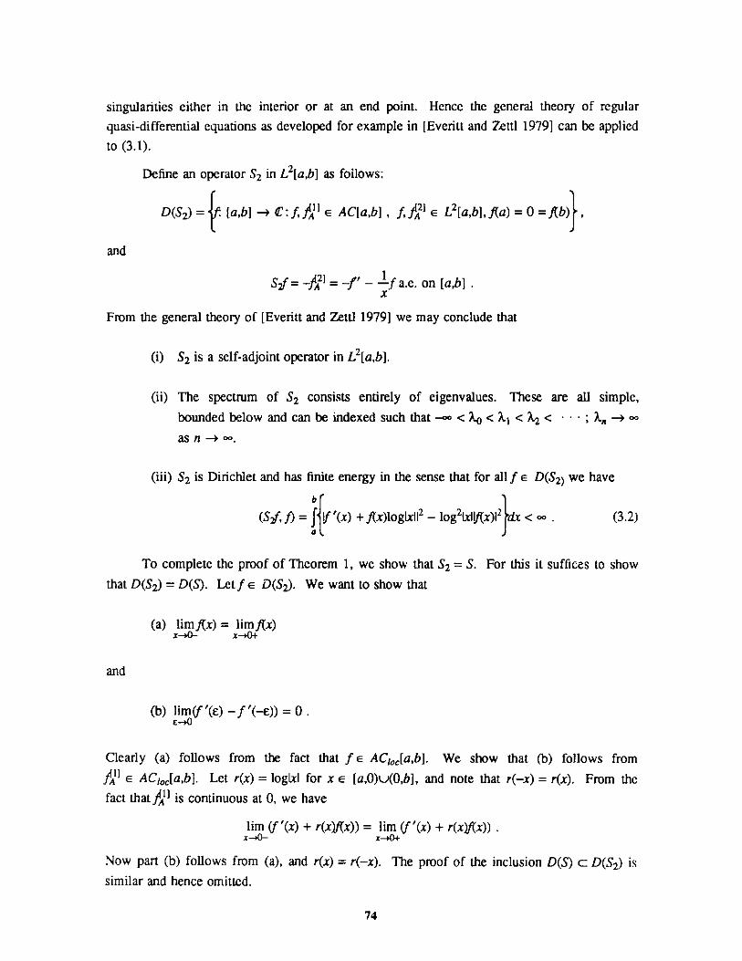
singularities either in the interior or at an end point. Hence the general theory of regularquasi-differential equations as developed for example in [Everitt and Zettl 1979] can be appliedto (3.1).
Define an operator S2 in L2 [a,b] as follows:
D(S 2)={. [a,b] - C: f,Jfl E AC[a,b] , f, E L2[a,b],If(a) = 0 =f(b)},
and
S2f_= -j1 =-f' - -f a.e. on [a,b] .x
From the general theory of [Everitt and Zettl 1979] we may conclude that
(i) S2 is a self-adjoint operator in L 2 [a,b].
(ii) The spectrum of S2 consists entirely of eigenvalues. These are all simple,
bounded below and can be indexed such that - <X0 < X< < -2--"; X,, -+ cas n -+ oo.
(iii) S2 is Dirichlet and has finite energy in the sense that for allf e D(S2) we have
(S 2f, f) = f{!f'(x) + f(x)loglxlI 2 - log2lx2I(x)}dx< . (3.2)
To complete the proof of Theorem 1, we show that S2 = S. For this it suffices to show
that D(S2 ) = D(S). Let f e D(S2 ). We want to show that
(a) limffx) = limf(x)X-+,&- x-+#
and
(b) im(f '(e) - f '(-E)) = 0 .
Clearly (a) follows from the fact that f E AC 1,0 [a,b]. We show that (b) follows fromf e AC10 [a,b]. Let r(x) = loglxI for x e [a,0)u(0,b], and note that r(-x) = r(x). From the
fact that fi is continuous at 0, we have
lim (f '(x) + r(x)ftx)) = lim (f '(x) + r(x)f(x)) .X-+0- x-+0+
Now part (b) follows from (a), and r(x) = r(-x). The proof of the inclusion D(S) c D(S2 ) is
similar and hence omitted.
74
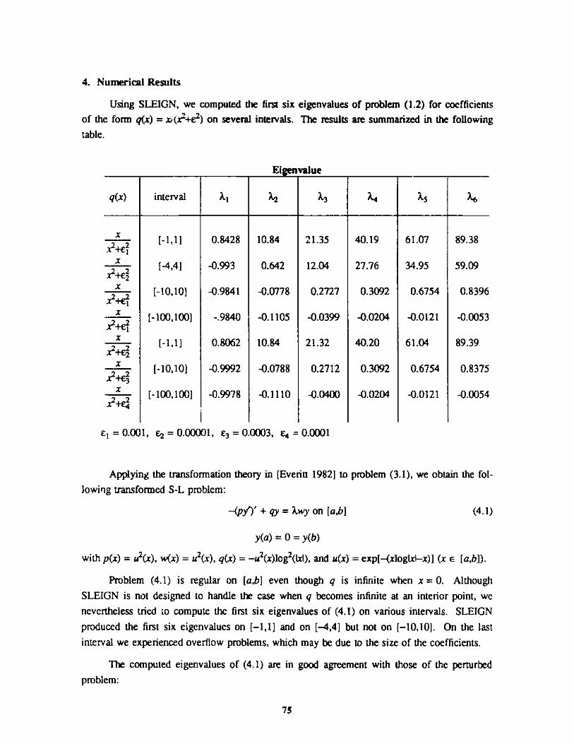
4. Numerical Results
Using SLEIGN, we computed the first six eigenvalues of problem (1.2) for coefficientsof the form q(x) = x(x2+e2) on several intervals. The results are summarized in the following
table.
Eigenvalue
q(x) interval A )2X3)4 X
x
x
x2+e2x
x
x2+E?
x
x
x
[-II,1]
[-4,4]
[-10,10]
[-100,100]
[-1,1]
[-10,10]
[-100,100]
0.8428
-0.993
-0.9841
-.9840
0.8062
-0.9992
-0.9978
10.84
0.642
-0.0778
-0.1105
10.84
-0.0788
-0.1110
21.35
12.04
0.2727
-0.0399
21.32
0.2712
-0.0400
40.19
27.76
0.3092
-0.0204
40.20
0.3092
-0.0204
61.07
34.95
0.6754
-0.0121
61.04
0.6754
-0.0121
89.38
59.09
0.8396
-0.0053
89.39
0.8375
-0.0054
E 1 = 0.001, E2 = 0.00001, 3 = 0.0003, E4 = 0.0001
Applying the transformation theory in [Everitt 1982] to
lowing transformed S-L problem:
-(py')' + qy = Xwy on [a,b]
problem (3.1), we obtain the fol-
(4.1)
y(a) = 0 = y(b)
with p(x) = u2 (x), w(x) = u2(x), q(x) = -u 2(x)log2 (Ixl), and u(x) = exp[-(xloglx--x)] (x e [a,b]).
Problem (4.1) is regular on [a,b] even though q is infinite when x = 0. Although
SLEIGN is not designed to handle the case when q becomes infinite at an interior point, we
nevertheless tried to compute the first six eigenvalues of (4.1) on various intervals. SLEIGN
produced the first six eigenvalues on [-1,1] and on [-4,4] but not on [-10,10]. On the last
interval we experienced overflow problems, which may be due to the size of the coefficients.
The computed eigenvalues of (4.1) are in good agreement with those of the perturbed
problem:
75
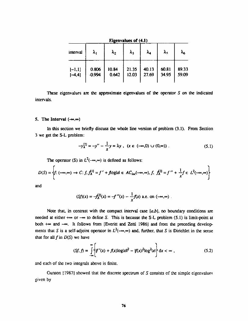
Eigenvalues of (4.1)
interval 7l 2 A 3 4j j___
[-1,1] 0.806 10.84 21.35 40.13 60.81 89.33[-4,4] -0.994 0.642 12.03 27.69 34.95 59.09
These eigenvalues are the approximate eigenvalues of the operator S on the indicated
intervals.
5. The Interval (-oo,oo)
In this section we briefly discuss the whole line version of problem (3.1). From Section
3 we get the S-L problem:
-y12 = -y - y=y, (x e (-oo,0) (0,oo)) . (5.1)x
The operator (S) in L2(-oooo) is defined as follows:
D(S) = (-oo,oo) -4 C:f/, =f' +floglxW e AC,(-co,oo),f, f9 =f" + f Le ox
and
(Sf)(x) = -I2](x) =-f "(x) - 1(x) a.e. on (-oo,oo).
Note that, in contrast with the compact interval case [a,b], no boundary conditions are
needed at either +0 or -m to define S. This is because the S-L problem (5.1) is limit-point at
both +co and -m. It follows from [Everitt and Zettl 1986] and from the preceding develop-
ments that S is a self-adjoint operator in L2(-oo,oo) and, further, that S is Dirichlet in the sense
that for all fin D(S) we have
(Sf, f) = 1{f'(x) +f(x)loglxl 2 - it(x)12log2Wdx < , (5.2)
and each of the two integrals above is finite.
Gunson [1987] showed that the discrete spectrum of S consists of the simple eigenvalues
given by
76
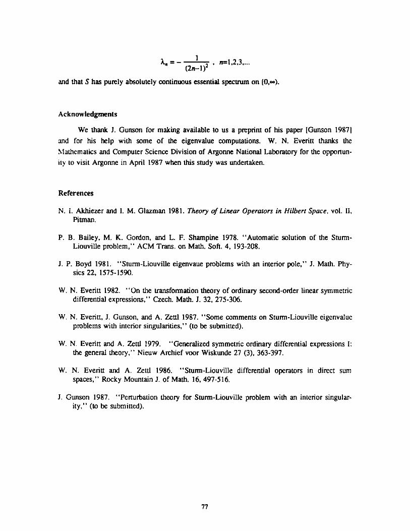
k.= - 1 =,,,.
(2n-1) 2
and that S has purely absolutely continuous essential spectrum on [0,mc).
Acknowledgments
We thank J. Gunson for making available to us a preprint of his paper [Gunson 19871
and for his help with some of the eigenvalue computations. W. N. Everitt thanks the
Mathematics and Computer Science Division of Argonne National Laboratory for the opportun-
ity to visit Argonne in April 1987 when this study was undertaken.
References
N. I. Akhiezer and I. M. Glazman 1981. Theory of Linear Operators in Hilbert Space, vol. II,Pitman.
P. B. Bailey, M. K. Gordon, and L. F. Shampine 1978. "Automatic solution of the Sturm-Liouville problem," ACM Trans. on Math. Soft. 4, 193-208.
J. P. Boyd 1981. "Sturm-Liouville eigenvaue problems with an interior pole," J. Math. Phy-sics 22, 1575-1590.
W. N. Everitt 1982. "On the transformation theory of ordinary second-order linear symmetricdifferential expressions," Czech. Math. J. 32, 275-306.
W. N. Everitt, J. Gunson, and A. Zeal 1987. "Some comments on Sturm-Liouville eigenvalueproblems with interior singularities," (to be submitted).
W. N. Everitt and A. Zettl 1979. "Generalized symmetric ordinary differential expressions I:the general theory," Nieuw Archief voor Wiskunde 27 (3), 363-397.
W. N. Everitt and A. Zettl 1986. "Sturm-Liouville differential operators in direct sumspaces," Rocky Mountain J. of Math. 16, 497-516.
J. Gunson 1987. "Perturbation theory for Sturm-Liouville problem with an interior singular-ity," (to be submitted).
77
ASYMPTOTICS OF THE TITCHMARSH-WEYLm-COEFFICIEN f FOR NONINTEGRABLE POTENTIALS
F. V. Atkinson'Department of Mathematics
University of TorontoToronto, Ontario M5S IAl, Canada
C. T. FultontDepartment of Applied Mathematics
Florida Institute of TechnologyMelbourne, Florida 32901
Abstract
Asymptotic formulae for the Titchmarsh-Weyl m-coefficient on rays in thecomplex ?-plane for the equation -y" + qy = Xy when the potential is limit cir-cle and nonoscillatory at x = 0 are obtained under assumptions slightly moregeneral than xq(x) e L1 (0,c). The behavior of q at the right endpoint is arbi-trary and may fall in either the limit point or limit circle case. A method ofregularization of the equation is given that can be made to depend either on asolution of the equation for X = 0 or more directly on an approximation to thesolution in terms of q. This enables equivalent definitions of the m-coefficientto be given for the singular Sturm-Liouville problem associated with a singularlimit circle boundary condition, and its associated regular Sturm-Liouville prob-lem. As a consequence, it becomes possible to apply asymptotic resultsobtained by Atkinson [1981] for the regular problem in order to give asymp-totic results for the singular problem. Potentials of the form q(x) = Cx',1 j< 2, are included. In the case j = 1 an independent calculation of thelimit point m-coefficient over the range (0,oo) relying on Whittaker functionsverifies the main result.
1. Introduction
The Titchmarsh-Weyl m-coefficient occupies, together with the spectral function, a central
place in the theory of the differential equation
y"+(A--q)y=0, O<x<oo, (1.1)
and of generalizations such as
y" + (Xw-q)y =0, (1.2)
Senior Mathematician Emeritus at the Mathematics and Computer Science Division, Argonne National Lab-oratory, October 1, 1986 to July 17, 1987.
tParticipantin Faculty Research Leave at Argonne Program, Mathematics and Computer Science Division,
Argonne National Laboratory, April-June 1987.
79
(py')' + (Xw-q)y = 0.
A survey of developments in the area up to 1980 may be found in [Everit and Bennewitz
19801; an updated version is in preparation. Our concern here is with the asymptotics of this
function which have, on the mathematical side, provided a method of estimating the spectral
density, as in the classical work of Titchmarsh [19621, and numerous more recent investiga-
tions [Atkinson 1982; Harris, 1985; Hinton and Shaw 1984 and 19861. Estimations of this
function have recently proved of relevance in certain problems of chemical physics [Hehen-
berger, Froelich, and Brandas 1976; Hehenberger, Laskowski, and Brandas 1976].
These asymptotics have been highly developed for the case of (1.1) with q absolutely
integrable near x = 0, so that
qE L1 (0,c), 0<c<o. (1.4)
The leading term in the approximation was obtained by Everitt [19721 (also for certain cases of
(1.3) with w(x) = 1). A further term in the approximation was obtained by Atkinson [19811.
The topic has been substantially developed in a recent series of papers by Harris [1984, 1985,
1986a, 1986b, 1986c], in which higher-order approximations are found, depending on the
degree of regularity of q. Simplified proofs of the results in [Atkinson 1981; Hams 19841
have recently been given by Kaper and Kwong [1986]. The case of (1.2) or (1.3), with a non-
constant weight-function tending to 1 as x - 0 has been dealt with, so far as the leading term
is concerned, by Everitt and Halvorsen [19781; a further term was obtained in [Atkinson 19811.
The case in which w(x) behaves as xa, a > -1, has been treated recently by Halvorsen [19841.
The leading term for the case of (1.1) when the boundary condition involves linear dependence
on ? has been obtained by Fulton [1981].
In this paper we develop the asymptotics of the m-coefficient for (1.1) when q is permit-
ted to have a nonintegrable singularity at x = 0 of the form
q(x)=Cx-, 15j<2. (1.5)
Such potentials are of interest in quantum scattering theory; cf. [Newton 1966; Schechter
1981]. Atkinson and Fulton [1984] have obtained asymptotics of eigenvalues of (1.1) over the
finite interval [0,b] under hypotheses that included the case (1.5). As for the asymptotics of
m(X) a partial move was given in [Atkinson 1982, Section 3.2] in which nonabsolute integra-
bility of q near x = 0 was permitted. The case (1.5) has the features of being limit circle and
nonoscillatory at x = 0. On the other hand, the potential is singular in that solutions of (1.1)
need not have finite derivatives at x = 0. For this reason it becomes necessary for the
definition of solutions that become involved in the definition of the m-coefficient to have
recourse to "boundary values" [Dunford and Schwartz 1963, p. 12971 at the limit circle end-
point or to rely on a regularizing transformation as in [Atkinson and Fulton 1984].
80
(1l.3 )
The various approaches to defining the m-coefficient and the matter of its dependence on
the choice of "boundary values" or regularizing function will be discussed in Section 2. The
main result will be given in Sections 3 and 4. In Section 5 we apply our result for the m-
asymptotics to the cases (1.5), and in Section 6 we give an independent verification based on
the use of Whittaker functions for the Coulomb case, j = 1.
In this paper we allow a slightly larger class of admissible potentials than in [Atkinson
and Fulton 1984]. For arbitrary c > 0 we put
C
q1 (x) = -J'q(t)dt (1.6)X
q2 (x) = gi(t)dt , (1.7)
and make the following basic assumptions for potentials q which are continuous in (0,oo):
q2(x) exists at least as an improper Riemann Integral (1.8)
and
tqi(t) E L1(0,c) (1.9a)
for some c > 0, or, equivalently,
C
5q(s)ds E L (0,c) . (1.9b)
The equivalence of these assumptions is readily established by an integration by parts which
gives
C C C C-X
JJqi(s)dsdt = (t-x)qi(t)dt = Jsq(s+x)ds.X c x S=O
By letting x -+ 0 and using suitable Lebesgue convergence theorems, it follows that (1.9a)
implies (1.9b) and vice versa and, moreover, that
C
limxfq (t)dt = 0 . (1.10)x-+0 x
The assumptions (1.8),(1.9) are sufficient to guarantee that (1.1) satisfies the following property
that we shall term "Property B," for which the value of A e (-oooo) is immaterial. We ask
that
u"-q(x)u=0,0<x<oo, (1.11)
should have a solution u(x) such that
81
limu(x) = I (1.12)X-+0
In fact, we have the following generalization of Lemma 1 of [Atkinson and Fulton 1984]:
LEMMA 1.
(i) Let (1.8),(1.9) hold. Then Property B holds. Also, under the assumption (1.8), the
requirement (1.9) is necessary for Property B. Moreover, for any solution u satisfying (1.12),
we have
u(x) = exp(q2 (x)) + 0 [g j(s)ds dt (1.13)
and
u'(x) = q1(x)exp(q2 (x)) + O0 gj(s)ds + Iqi(x) fgi(s)ds dt (1.14)
for any c > 0.(ii) In the special case of
q(x) e L1 (0,c) , (1.15)
for some c > 0, the solution u satisfying (1.12) can be selected in a unique way to give the fol-
lowing improved error bounds:
u(x) = exp(q2 (x)) + 0[I[ qi(s)ds dt = I + q2 (x) + 0 x q (s)ds (1.16)
and
u'(x) = q1(x) + 0 [q(s)ds 1 + xIlq(x) . (1.17)
Proof of (i). Modifying the method of [Atkinson and Fulton 1984], we choose a solution U of
(1.11) defined by the initial conditions
U(S) = I , U'(S) = q1 () , (1.18)
and show that if 8 > 0 is small enough, then U(x) tends to a positive limit U(O) as x -+ 0.
Making the change of variable
V(x) = U(x)exp(-q2(x)) (1.19)
in (1.11), we obtain
82
(exp(2q 2)V(x))' + qgexp(2q2)V(x) = 0 ,
and upon integration using (1.18),
8
V(x) = exp(-2q2(x))Jexp(2q2 (t))qi(t)V(t)dt . (1.21)X
Here the exponential terms are bounded for S E (0,c), so there exists a bound of the form
8
IV(t)l S Kgf(s)IV(s)Ids . (1.22)
Integrating over [x,S], S < c, and using an integration by parts on the righthand side gives
8
xIV(x)-V(8) S K f(t-x)q(t)V(t)dt (1.23)
8
a<_ K ftq (t) V(t) dt .
By the Gronwall inequality we therefore have fur all x e [0,6]
IV(x)I V(8)exp K tqt)dt . (1.24)
Hence if S is chosen so small that
K tg1(t)dt < '/ , (1.25)
we have from (1.22),(1.23) that
V(8)(1 - '/ed) IV(x)I e V(S) (1.26)
for all x e [0,8], where V(S) = exp(-q2 (8)). This shows that V(x) is bounded from below and
also from above in (0,8). It also follows by integration of (1.22) that V(x) is of bounded varia-
tion over (0,S) and that V(x) therefore tends to a limit V(0) as x -+ 0, which must be positive
by (1.22). It then follows that U(x) tends to a positive limit U(0) as x -+ 0, so we have
proved the sufficiency of the criteria (1.9) for the existence of u(x); we have only to put
u(x) = U(x)/U(0) . (1.27)
To prove (1.13), we take S fixed as above and integate (1.21) over [0,x] to obtain
V(x) = U(0) +0 gj(s)ds dt . (1.28)
83
(1.20)
Since
u(x) = U(x)/U(0) = V(x)exp(q 2(x))/U(0) ,
the result (1.13) follows immediately. We remark that an integration by parts making use of
(1.10) can be used to write the error term in the alternative form
fq(s)ds dt = tq (t)dt + x q (t)dt . (1.29)
To obtain (1.14), we observe from (1.19) that
U'(x) = exp(q2 (x))V'(x) + q1(x)U(x) . (1.30)
The first term gives rise to the first error term in (1.14) because of (1.22), and substitution of
the result for U(x) from (1.28) in the second term gives the other terms in (1.14).
To prove the necessity of the condition (1.9), we suppose q2(x) exists in (1.7) and let u(x)
be a solution of (1.11) which satisfies (1.12). Defining W(x) by
W(x) = exp(-q2 (x))u(x) , (1.31)
we find by integrating (1.20) over [x,c] that
C
W'(x) = exp(-2q2 (x) + 2q2 (c))W'(c) + exp(-2q2 (x))fqt(0exp(q2 (t))u(t)dtX
- q (t)dt, (1.32)X
C
as x -+ 0. If q (t) e L1(0,c) we have (1.9), so we assume that fq (t)dt -+ 0 as x -+ 0.X
Integrating (1.32) over [x,c] gives
C C
W(x) J Jfq(s)dsdt. (1.33)
Hence if (1.9b) were false, it follows that W(x) -+ oo as x -+ 0, which contradicts (1.31) (since
u(x) -+ 1 by assumption).
Proof of (ii). The proof of part (ii) is easier since (1.20) is regular at x = 0 and the basic solu-
tion may therefore be defined by the initial data V(0) = 1, V'(0) = 0; the integrations
corresponding to (1.21),(1.22),(1.23) may then be done over [0,x], and the result follows
without the need for a Gronwall argument.
84
It follows from Lemma 1 that (1.11) is nonoscillatory at x = 0 under the basic assump-
tions (1.8),(1.9). Since it is also limit. circle at x = 0, it follows that (1.1) is nonoscillatory for
all real X. Lemma 1 represents r specialization of a standard theorem on principal and
nonprincipal solutions at nonoscillatory endpoints; cf. [Hartman 1964, p. 355]. Letting u be
any nonprincipal solution satisfying (1.12), we define a linearly independent solution by
x
v(x) = u(x) 2Ldt . (1.34)1u2(t)
Since by (1.12) u(x) = 1 + o(l), it follows by putting this in (1.34) that
v(x) = x + o(x) , as x -40 . (1.35)
The solution v(x) is the principal solution which is unique up to a constant multiple; moreover,
the normalization (1.35) arising from (1.12) and (1.34) fixes the arbitrary constant, so that
(1.34) gives a uniquely defined principal solution. On the other hand, the nonprincipal solution
in (1.13) is not unique because it contains an error term big enough to include the principal
solution.
For the purpose of introducing a parametrization of the m-coefficients associated with
different limit circle boundary conditions at x = 0, it will be helpful to introduce a canonical
choice of the nonprincipal solution. This can be done as follows: from (1.13) and (1.35) it
follows that any nonprincipal solution satisfying (1.12) may be written in the general form
u(x) = 1 + intermediate + a + lower order,(1.36)order terms terms
where the constant a represents a measure of the linear dependence of u on v. Accordingly, a
natural choice of nonprincipal solution can be obtained by requiring that a = 0 in the represen-
tation (1.36). This uniquely fixes the choice of nonprincipal solution, since it fixes the depen-
dence of u on v. Henceforth we let u(x) denote this canonical choice of nonprincipal solution.
With this choice, the family of all nonprincipal solutions of (1.11) which satisfy (1.12) may be
parametrized in the form
u(x) = u(x) + (cot a)v(x) , a e (0,i) . (1.37)
Under the restrictive assumption (1.15), we can make use of (1.16) and (1.17) in (1.34)
to get an improvement over (1.35). This gives the following lemma.
LEMMA 2. Assume that (1.15) holds. Then for the principal solution defined by (1.34) we
have
85
v(x) = x + xq2(x) - 2 q2 dt + 0 x2[I (s)s] (1.38)
and
x
v'(x) = 1 + xq1 (x) - q2(x) - 2g(x) q2(t)dt
x
+ O x (s)ds 1 + x gl(x) . (1.39)
REMARK 1.1. The proofs of Lemmas 1 and 2 do not depend in any essential way on the
choice of X = 0. Principal and nonprincipal solutions satisfying (1.12) and (1.35) (and there-
fore a canonical nonprincipal solution with a = 0 in (1.36)) necessarily exist for all real values
of X, and Lemmas 1 and 2 remain in force under the replacement q - q-, X e (-o,oo), in
(1.11) and in the basic definitions (1.6),(1.7). The basic assumptions (1.8),(1.9) remain the
same.
The basic assumptions (1.3),(1.4) of [Atkinson and Fulton 1984] imply the conditions
(1.8),(1.9) (and, in particular, the absolute integrability of the integral (1.7) defining q2(x)), but
not vice versa. The present assumptions (1.8),(1.9) cover certain "wildly oscillating" poten-
tials such as
q(x) = x"sin(x"'), with m> n-2, (1.40)
or
q(x) = x-2lnx sin(x-) , (1.41)
which do not satisfy the assumptions of [Atkinson and Fulton 1984]. Similarly, the limit rela-
tion (1.5) of [Atkinson and Fulton 1984] implies (1.10) but not vice versa. However, we have
the following lemma which provides ai analogue for (1.5) of [Atkinson and Fulton 1984]; this
covers certain oscillatory potentials such as (1.40),(1.41).
LEMMA 3. Let (1.8),(1.9) hold, and in addition suppose that
C
lim Jtq(t)dt, c > 0 , (1.42)E-+E
exists as an improper Riemann Integral. Then
f(x) = xq1 (x) -+ 0 as x ->0 . (1.43)
Proof An integration by parts gives
86
q2(y) - q 2 (x) = q1(t)dt = fty) - fx) - ftq()dt.X x
Letting x -+ 0 gives
lim [(x) + ft(t)dt] =fly) - q2 (y) . (1.44)x-0 x
The existence of the limit in (1.42) thus implies the existence of
L h:=j x) (1.45)
and vice versa. Moreover (1.42) and (1.44) imply
L =fly) - q2(y) - Jtq(t)dt (1.46)
for all y > 0. To show that L = 0, we observe that L is independent of the choice of the upper
limit c in the definition (1.6) of q1(x). Given e > 0, we choose 5 > 0 small enough so that
1q2(5)I + tq(t)d] < e.
Then, letting q1(x) be defined by
q1(x) = -Jq(t)dt ,
we have f(S) = 0, so that with y = 8 in (1.46) we get
ILI = q2() + Itq(t)d] < e.
q.e.d.
REMARK 1.2. If (1.8),(1.9) and (1.42) hold, then it follows from (1.14) and Lemma 3 that
C
xu'(x) = xq(x)(l+o(1)) + O x qs)ds (1.47)
so that we also have xu' -+ 0 as x -+ 0.
REMARK 1.3. There is an analogue of Lemma 1(i) that was not stated in [Atkinson and Fulton
1984]. Specifically, if q(x) is of fixed sign in a neighborhood of x = 0, then (1.3) or (1.10) of
87
[Atkinson and Fulton 1984] are necessary and sufficient conditions for "Property A" of
[Atkinson and Fulton 1984].
2. Transformation to a Regular Sturm-Liouville Problem
We associate with the singular equation (1.1) a limit circle boundary condition at x = 0 of
the form
B(y,u) = 0 , (2.1)
where
B(fu) = limW,(fu) = lim(fu'-fu) (2.2)x-.0 x-+0
is a "boundary value" for (1.1) at x = 0. In particular, if u is taken as the solution (1.37) of
(1.11), then as in [Atkinson and Fulton 1984], the class of all admissible boundary conditions
at x = 0 may be parametrized in the form
sin a B(y,u,) + cos a B(y,v) = 0, a E [0,n) . (2.3)
Probably the simplest approach to the asymptotics of the m-coefficient is to make a
change of variable in (1.1) which brings the equation into the form of a regular Sturm-Liouville problem, and the singular boundary condition into a standard regular boundary condi-
tion. This method of attack is a relatively recent phenomenon; in [Atkinson and Fulton 1984]
we used a regularizing transformation that depended on a solution of (1.11) in a neighborhood
of zero to study the asymptotics of eigenvalues of (1.1),(2.3), and Kaper, Kwong, and Zettl
[1984] used a regularizing transformation for certain limit-circle problems that depended
directly on the coefficient functions of the singular Sturm-Liouville problem. The changes of
variable have to be carefully chosen so as not to alter the spectral quantities under investiga-
tion. In this paper we adopt a hybrid procedure in which the method of regularization may
depend either on a solution of (1.11) or more directly on the potential q.
Similarly to [Atkinson and Fulton 1984] we make the change of variables
x
t = u ds , Y(t) = y(x)/u(x) (2.4)u2(s)
under which (1.1) transforms to
d Y + [Xu t(x) - u3(x)(q(x)u(x) - u"(x))]Y = 0 . (2.5)dt2
Here x = x(t) is the inverse of the function defined in (2.4). In the case that u is taken as a
solution of (1.11), this reduces to
88
d 2Y--- + u(x)Y= 0. (2.6)dt 2
On the other hand, if we allow u(x) to be any positive function such that
limu(x) = 1 (2.7)x-O
and
u" - qu e L1(0,c) (2.8)
for some c > 0, then the new equation (2.5) is regular at x = 0 and falls in the case (1.2) with
w(x) -* 1 as x -+ 0 and q satisfying (1.4). Accordingly, the leading term in the expansion of
the m-coefficient associated with (2.5) is available from [Everitt and Halvorsen 1978] and
[Atkinson 1981]. Moreover, we shall be able to apply the results of Atkinson [1981] without
essential change to obtain a second order term.
The change of dependent variable in (2.4) requires that u be positive over the range
where (2.5) is to be used. We may, for example, take u to be a solution of (1.11) satisfying
(1.12) which is positive in a neighborhood of x = 0 and let it be continued so as to be positive
over (0,oo) as in [Atkinson and Fulton 1984], or we may take u to be an "approximate" solu-
tion that satisfies (2.8). In either event, the behavior of u away from x = 0 will be immaterial
for our purposes since the m-asymptotics will be determined solely by the behavior of u in a
neighborhood of x = 0. An "approximate" solution suitable for use in (2.4) is suggested by
Lemma 1, namely,
u(x) = exp(q2(x)) . (2.9)
In this case we have
u" - qu = q(x)exp(q 2(x)) , (2.10)
so that the requirement (2.8) holds only under the restrictive assumption (1.15). For the case
(1.5), this supplies a regularizing function u valid for the range 1 j < 3/2.
LEMMA 4. Let u be a nonprincipal solution of (1.11) satisfying (1.12) or a regularizing func-
tion satisfying (2.7),(2.8).
(i) Then the boundary condition (2.1) transforms under the change of variable (2.4) to the
Neumann boundary condition
Y'(0) = 0 . (2.11)
(ii) Let v be the principal solution (1.34) of (1.11). Then the Friedrichs boundary condition at
x = 0 for (1.1) may be written as
B(y,v) = y(0) = 0 , (2.12)
89
and it transforms under (2.4) (when u is a nonprincipal solution) to the Dirichlet boundary
condition
Y(0) = 0 . (2.13)
(iii) Let (1.15) hold. Assume that the constant c in (1.6) is chosen so that q2(x) has no term of
order ax (and hence that (1.16) is the canonical nonprincipal solution). If
u = I + q2(x) + (cot a)x , a E (0,n) , (2.14)
is used in (2.4), then the boundary condition (2.1) is equivalent to (2.3), i.e.,
sin a B(y,1+q2) + cos c B(y,x) = sin a B(y,uc) + cos a B(y,v) (2.15)
for all solutions y of (1.1).
Proof of (i) and (ii). By (2.4) we 'lave the relations
Y(t) = y(x)/u(x) , Y(t) = u(x)y'(x) - u'(x)y(x) (2.16)
relating solutions of (2.5) or (2.6) to those of (1.1). If we let t -* 0, it follows that
Y(0) = y(0) and Y'(0) = B(y,u) , (2.17)
where B(y,u) is the u-dependent Wronskian limit in (2.2). The existence of this limit for all
solutions y of (1.1) can be inferred from the fact that all solutions of (2.5) or (2.6) are continu-
ous and have continuous derivatives at t = 0. Similarly, existence of the limit y(x) -+ y(O) for
all solutions of (1.1) follows by letting t -+ 0 in the rirst part of (2.16). In the case when u is
not a solution of (1.11) it should be checked that the Wronskian limit in (2.2) does in fact exist
for all f in the domain of a suitable maximal operator, so that (2.1) is a "boundary value" for
(1.1) in the sense of Dunford and Schwartz [1963, p. 1302, Theorem 271. For the sake of
argument we suppose that x = o is limit point and let D,D denote the domains of the maximal
operators associated with (1.1) and (2.5), respectively. It is readily verified that the same
change of variables (2.4) used to bring (1.1) into the regularized form (2.5) defines a one-to-
one mapping of y e D onto Y E D. Accordingly, (2.16),(2.17) hold for y E D and Y e D.
It follows that the Wronskian limit in the second part of (2.17) exists for al! y e D and is
therefore a boundary value for (1.1); similarly, since all elements of D are continuous at t = 0,
it follows from the first part of (2.17) that all elements of D are also continuous at t = 0 and
that B1(y) = y(O) is a boundary value for (1.1). Accordingly, B1(y) = y(O) and the Wronskian
limit -B(y,u) are the "boundary values" for the singular equation (1.1) which are transformed
under the change of variable (2.4) to the boundary values Y(0) and Y'(0), respectively, of the
regular equation (2.5) or (2.6). It remains to prove (2.12). Under the hypothesis of Lemma 3
it follows by differentiating (1.34) and using (1.47) that the principal solution satisfies
90
By the A-dependent analogue of Lemma 3 it follows that xy'(x,X) -* 0 as x -+ 0 for any
nonprincipal solution of (1.1) for X real. Hence
B(y,v) = limyv' = y(O) (2.19)x-+O
for all solutions of (1.1), so the boundary value, B(y) = y(0), is identified as the Wronskian
limit with the principal solution. Putting (1.34) in (2.19) and using (1.12) and (1.47), we see
that (2.19) reduces to Rellich's characterization of the Friedrichs boundary condition; cf. [Rel-
lich 1951, pp. 354-3551. q.e.d.
Proof of (iii). The regularizing function (2.14) is constructed from the leading terms in (1.16)
and (1.38). The proof of (2.15) makes use of Lemma 1(ii), Lemma 2, and their A-dependent
analogues.
Note: For arbitrary choices of u satisfying (2.7),(2.8), it does not appear possible to give a
natural parametrization of the boundary ccadition (2.1).
We now describe the manner in which the m-coefficient associated with (1.1) and the
singular boundary condition (2.1) remains invariant under the change of variables (2.4).
To define the m-coefficient associated with (2.5) and the Neumann boundary condition
(2.11), we let 0 and 8 be defined for all A E C (C = complex numbers) as solutions of (2.5)
by the initial data
(0,X) = -1 , 0'(0,A) = 0 , 9(0,A) = 0 , 0'(0,x) = 1 , (2.20)
and put
M7,,(k ; ) = - '' .(2.21 )- )(T,) - EI'(T,X)
This m-coefficient depends on the choice of u in (2.4). Using the terminology of [Atkinson
1981], we let, for any nonreal A = k2, the circle that is the image of the real 4-axis under the
mapping (2.21) be denoted by C(T,k) and the corresponding disk that it encloses by D(T,k).
Although the practice is not widespread in the literature, it is possible to introduce an m-
coefficient associated with the singular equation (1.1) and the singular boundary condition (2.1)
by making use of the two singular "boundary values" in (2.17). A general approach of this
type for two singular endpoints with the left endpoint being L.C. was taken in [Fulton 19801.
Following that method, we define solutions $ and 0 of (1.1) for all A E C by the initial data
(singular "end conditions" in the terminology of [Fulton 1977 and 19801),
91
v'(0) = I . (2.18)
$(OX) = I , B($(,X),u) = 0 , 0(0,?) = 0 , B(0(-,X),u) = -l ,2
and put
mxyAQt) = -0(X,?) - k0'(XX)(
$(Xx) - $'(X, ) J(2.23)Let, for nonreal X = k2, c(X,k) denote the circle that is the image of the real t-axis under
(2.23) and d~(X,k) the disk it bounds. If one wishes, one can develop the eigenfunction expan-
sion theory associated with (1.1),(2.1) and a singular right endpoint (of L.P. or L.C. type) by
following the analysis of Chapters 2 and 3 of Titchmarsh's book [Titchmarsh 1962] with the
4)- and 0-functions and the lb-function replaced throughout by the corresponding 4)- and 0-
functions and mx-function defined in (2.22),(2.23). Our aim here, however, is to treat the regu-
larized equation (2.5) directly and translate results back to the singular equation. To this end
we prove the following lemma.
LEMMA 5. Let r be a solution of (1.11) satisfying (1.12), or a regularizing function satisfying
(2.7),(2.8). Then the real t-axis maps onto the same circle under the linear fractional map-
pings (2.21) and (2.23), where T and X are related by (2.4); that is, for fixed u we have for all
X with ImK # 0
C=c~ and D=d. (2.24)
Proof. Comparing (2.22) and (2.20), we see that the solutions 4),0 are related to (D,e by
$x,x) = u(x)0D(t,X) , 0(x,) = u(x)0(t,) , (2.25)
that is, by the change of variable (2.4). Substituting this into (2.21) and making use of the
second relation in (2.16), we find that the m-coefficients are related by
Mrs(.;t) = mx,(K;() , (2.26)
where
x
T = 2( ds , (2.27)
and the 1-1 correspondence between t E (-oo,oo) and E (-oo,oo) is given by
((4) = tu2 (X) / (1 + tu(X)u'(X)) . (2.28)
q.e.d.
92
(2.22)
3. The Main Result
The main idea is to apply a suitably adapted version of Theorem 3 of [Atkinson 19811 to
the regularized equation (2.5) to obtain asymptotic results for the m-coefficient (2.21) associ-
ated with (2.5) and the Neumann boundary condition (2.11). To the order of accuracy we shall
obtain, the asymptotics will be the same regardless of whether we consider a Sturm-Liouville
problem over a finite interval or over a singular interval; moreover, the behavior of q(x) at -c
may be completely arbitrary, falling in either the limit point or limit circle case. Since the cir-
cles Cu(T,k) and c(X,k) under the mappings (2.21) and (2.23) are identical, it follows that
asymptotic results for the regular equation will be valid also for the singular equation (1.1).
In this section we allow the regularizing function u(x) to be either a solution of (1.11) or
a function satisfying (2.7),(2.8). In Section 5 we address the matter of applying the asymptotic
results to some examples. We write the regularized equation (2.5) in the form
d2 Y/dt2 + ( - Q(t)Y) = 0 , (3.1)
where
Q(t) := k2(l - u4(x)) + u3 (x){q(x)u(x) - u"(x)) , (3.2)
and let n 1 = 71(T), 712 = 112() be defined by
T1 (T)= sup ew-r)Q(t)d (3.3)
T
312 (T)= esu rQ(t)d". (3.4)
We quote Theorem I of [Atkinson 1981] in the context of (3.1) and (2.20).
THEOREM 1. Let k = = a+ip, a > 0, where the branch is taken on the positive real X-axis.
Let T E (0,oo) be such that the following assumptions hold:
alePT> 251kl , (3.5)
11 1(T),11 2(T) < (1/8)min(cxl,$) , (3.6)
0<cE argX5n-e,or +e argX52n-E, (3.7)
Then every m e D.(T,k) satisfies, as IkI -+ o in the sectors defined by (3.7),
93
T
m - ilk - 1I/k e2aQ(t)dt = O(12(7)IkV3 ) + O(Ikrle-aT) . (3.8)
Note: Because the sectors (3.7) map onto sectors in the k-plane that are bounded away from
the real and imaginary k-axes, it follows that in these sectors Iki, 3 and lal tend to oo at the
same rate.
Since the leading term in Q(t) is of order k2 as k -+ o, it will not be possible to satisfy
the aSsumption (3.6) with a fixed value of T > 0. We therefore follow a procedure similar to
the proof of Theorem 3 of [Atkinson 1981] by making T = Tg -* 0 as $ -+ 00. However, we
adapt the analysis to the special c4-.. of (3.2). To ensure that the assumption (3.5) holds, we
require that pT -4 -o. For convenience we also let -XP~ T be the corresponding x-value from
(2.4), i.e.,
xp
T = L(l/u2(s))ds . (3.9)
We define
0(x) := sup lu(s)-Il . (3.10)osrs
We may use Theorem I to prove the following theorem.
THEOREM 2. Let Tp,Xg satisfy the requirements
T -,Xp -0 (3.11)
-T4, Xp -+ . (3.12)
Assurme u(x) is a regularizing function satisfying (2.7),(2.8). Then every m e d(Xp,k) satisfies,
as ikl -+00 in the sectors (3.7),
C Tg
m - i/k + 4te2"(u(x)-l)dx = 0 Ikr2 e2'lq(x)u(x)-u"(x)ldt (3.13)
xft x
+ 0 |kr2o(Xg) Iqu-u"ldx + ikr3 qu-u"dx
+ O(IkrF' 2(Xp)) + O(Iklre*)
Here c E (0,oo) is any fixed constant.
94
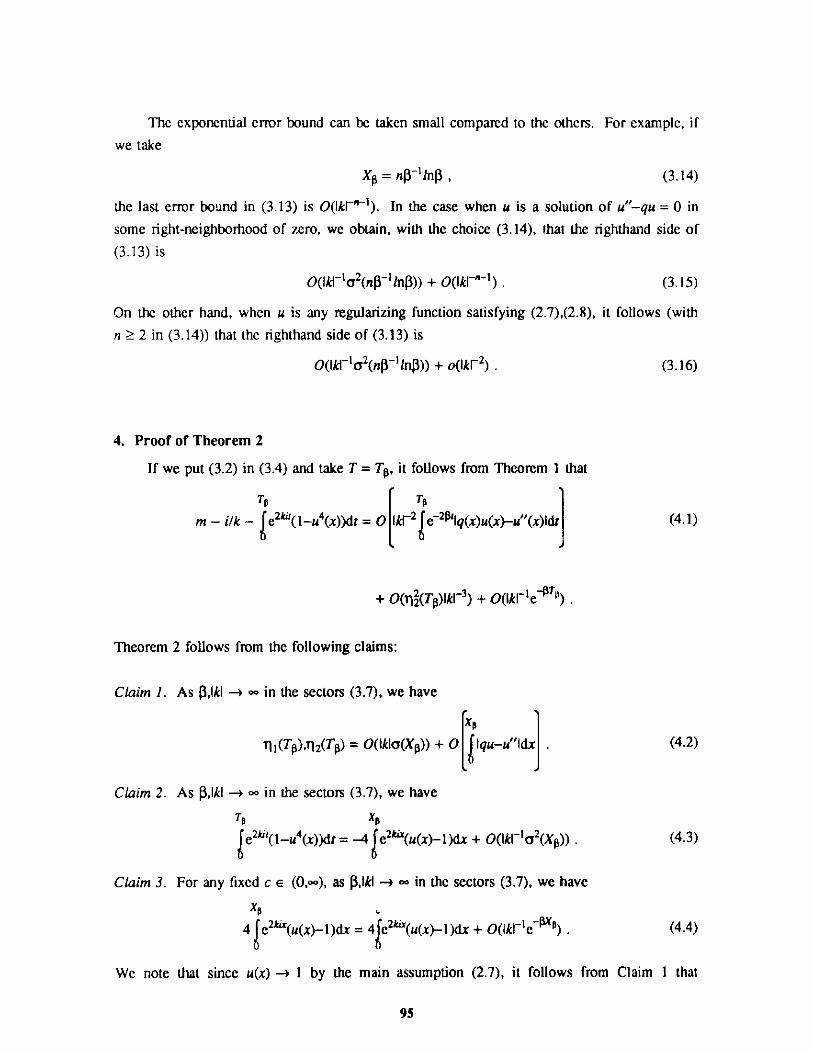
The exponential error bound can be taken small compared to the others. For example, if
we take
Xp = n@~'ln$ , (3.14)
the last error bound in (3.13) is O(Ikr"-1). In the case when u is a solution of u"-qu = 0 in
some right-neighborhood of zero, we obtain, with the choice (3.14), that the righthand side of
(3.13) is
O(IkF'a2(n4-'ln )) + O(Ik"~) . (3.15)
On the other hand, when u is any regularizing function satisfying (2.7),(2.8), it follows (with
n 2 in (3.14)) that the righthand side of (3.13) is
O(Ik-'a2(n$~'lnp)) + o(Ikr 2) . (3.16)
4. Proof of Theorem 2
If we put (3.2) in (3.4) and take T = T, it follows from Theorem 1 that
m - i/k - e 2s'( 1-u4 (x))dt = 01 IkW2 e~20hq(x)u(x) -u"(x)dt (4.1)
+ O(1(T)IkV3) + O(Ikr1e T )
Theorem 2 follows from the following claims:
Claim 1. As $,IkI -a 00 in the sectors (3.7), we have
x
rll(Tp),l2(Tp) = O(kla(Xp)) + 0 Iqu-u"Idx . (4.2)
Claim 2. As ,kl -+ o in the sectors (3.7), we have
e2 '(1-u4(x))dt = -4 e2 (u(x)_1)dx + O(Ikr'a 2(Xp)) . (4.3)
Claim 3. For any fixed c e (0,00), as $,Wlk -+ oo in the sectors (3.7), we have
x0
4 e2ki(u(x)-1)dx = 4Ie2 (u(x)-1)dx + 0(Ik'e0) . (4.4)
We note that since u(x) -+ I by the main assumption (2.7), it follows from Claim I that
95
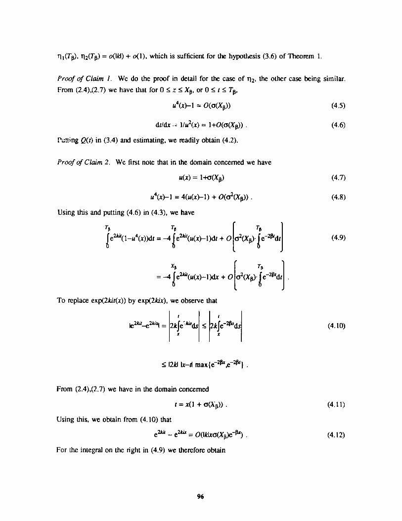
1i(TO), rl2(TT) = o(IkI)+ o(1), which is sufficient for the hypothesis (3.6) of Theorem 1.
Proof of Claim 1. We do the proof in detail for the case of 11 2, the other case being similar.
From (2.4),(2.7) we have that for 0 5 x _X p, or 0 t <-T,
u4(x)-1 = O(a(Xp)) (4.5)
dt/dx .= 1/u2(x) = 1+O(a(X)) . (4.6)
Putting Q(t) in (3.4) and estimating, we readily obtain (4.2).
Proof of Claim 2. We first note that in the domain concerned we have
u(x) = 1+o(Xp) (4.7)
u(x)-I = 4(u(x)-l) + O(&(Xp)) . (4.8)
Using this and putting (4.6) in (4.3), we have
T T T
e-4 pe4(x))dt = -41e"(u(x)-1)dt + T a2(Xp)- e-'dt (4.9)
= -4 e'"(u(x)-1)dx + 0 a2(Xp)-1e2pdt
To replace exp(2kit(x)) by exp(2kix), we observe that
I I
Ie2 '- eaI = 2ke-'ds < 2ke-2 ds (4.10)x x
12k1 x-ti max(e-2 x,e-')
From (2.4),(2.7) we have in the domain concerned
t = x(1 + a(Xp)) . (4.11)
Using this, we obtain from (4.10) that
ea' - e2a' = O(Ikxa(X)e~O") . (4.12)
For the integral on the right in (4.9) we therefore obtain
96
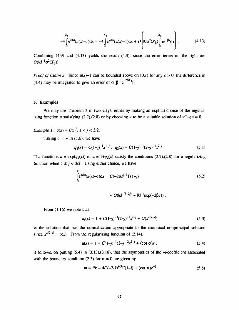
xa x0 x
-4e 2 '(u(x)-1)dx = -4 Ie"(u(x)-1)dx + 0 Ikl02(XP) Ixe~xdxJ. (4.13)
Combining (4.9) and (4.13) yields the result (4.3), since the error terms on the right are
O(Ikr~'o2(Xo)).
Proof of Claim 3. Since u(x)-1 can be bounded above on [O,c] for any c > 0, the difference in
(4.4) may be integrated to give an error of O($~'e~2 a).
5. Examples
We may use Theorem 2 in two ways, either by making an explicit choice of the regular-
izing function u satisfying (2.7),(2.8) or by choosing u to be a suitable solution of u"-qu = 0.
Example. q(x) = Cx~3, 1 < j < 3/2.
Taking c = oo in (1.6), we have
q1(x) = C(1-j)~'x'' , q2 (x) = C(1-j)~'(2JT)-x2-J . (5.1)
The functions u = exp(q2 (x)) or u = 1+q2 (x) satisfy the conditions (2.7),(2.8) for a regularizing
function when 1 -j < 3/2. Using either choice, we have
e2 (u(x)-1)dx = C(-2ikr3 (1-j) (5.2)
+ O(IkV-<- 2') + Ik'exp(-2 c))
From (1.16) we note that
ue(x) = I + C(1-j)-'(2-J'x2-+ O(x 2 2 -)) (5.3)
is the solution that has the normalization appropriate to the canonical nonprincipal solution
since x2 2 -)= o(x). From the regularizing function of (2.14),
u(x) = I + C(1-j)-'(2-j)-2i2-' + (cot a)x , (5.4)
it follows, on putting (5.4) in (3.13),(3.16), that the asymptotics of the m-coefficient associated
with the boundary condition (2.3) for a * 0 are given by
m = i/k - 4C(-2ikY 3F(l-j) + (cot a)k~2 (5.6)
97
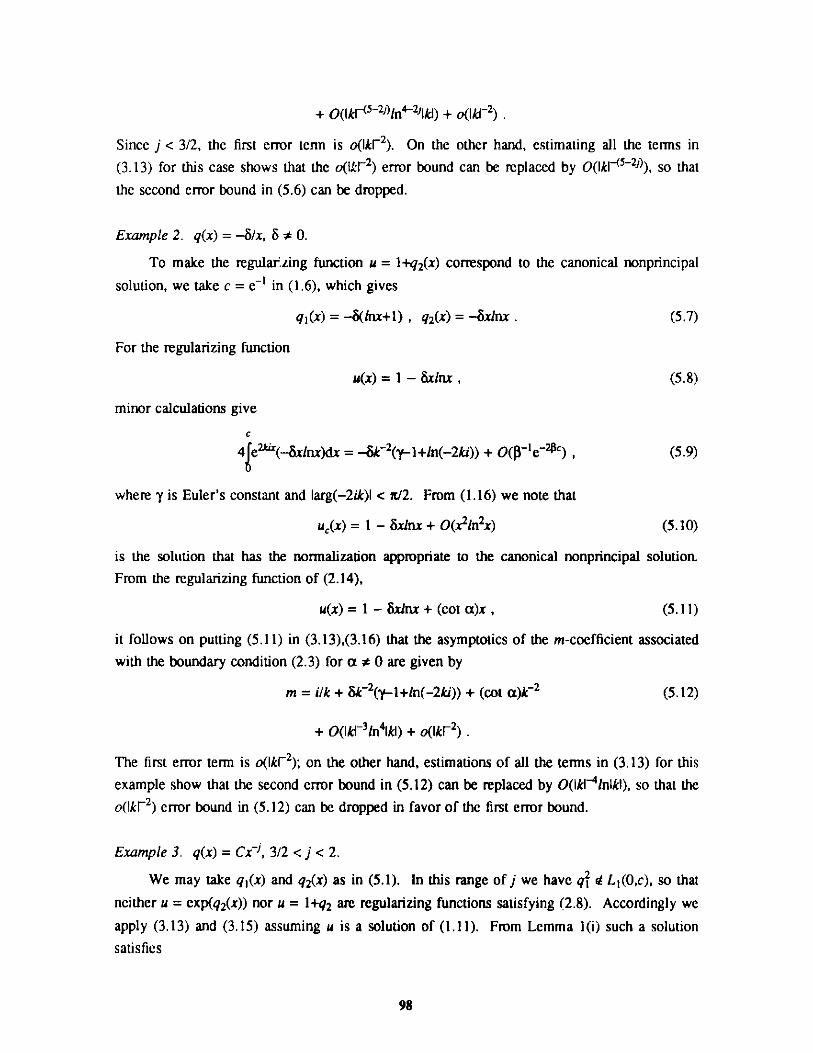
+ O(Ikr 5-2>ln4 -2jIkI) + o(IkF 2)
Since j< 3/2, the first error term is o(Ikr2). On the other hand, estimating all the terms in
(3.13) for this case shows that the o(Ikr 2) error bound can be replaced by O(Ik 5 2f>), so that
the second error bound in (5.6) can be dropped.
Example 2. q(x) = -6/x, S 0.
To make the regular.zing function u = 1+q2(x) correspond to the canonical nonprincipal
solution, we take c = e-1 in (1.6), which gives
q1 (x) = -5(Inx+l), q2 (x) = -xdnx . (5.7)
For the regularizing function
u(x) = 1 - xlnx , (5.8)
minor calculations give
C
4Ie2"(-xlnx)dx = -. k 2(t-1+ln(-2ki)) + O(~le2c) , (5.9)
where y is Euler's constant and Iarg(-2ik)I < i/2. From (1.16) we note that
uj(x) = I - 8xlnx + O(x2ln2x) (5.10)
is the solution that has the normalization appropriate to the canonical nonprincipal solution.
From the regularizing function of (2.14),
u(x) = 1 - 6xlnx + (cot a)x , (5.11)
it follows on putting (5.11) in (3.13),(3.16) that the asymptotics of the m-coefficient associated
with the boundary condition (2.3) for a * 0 are given by
m = i/k + Sk-2 ('?-l+In(-2ki)) + (cot a)k-2 (5.12)
+ O(IkF3ln4 \k) + o(Ikr 2).
The first error term is o(Ikr 2); on the other hand, estimations of all the terms in (3.13) for this
example show that the second error bound in (5.12) can be replaced by O(Ik 4I1nikI), so that the
o(Ikr2) error bound in (5.12) can be dropped in favor of the first error bound.
Example 3. q(x) = Cxf, 3/2 < j < 2.
We may take q 1(x) and q2(x) as in (5.1). In this range of j we have q 4 L1 (0,c), so that
neither u = exp(q2(x)) nor u = 1+q2 are regularizing functions satisfying (2.8). Accordingly we
apply (3.13) and (3.15) assuming u is a solution of (1.11). From Lemma 1(i) such a solution
satisfies
98
u(x) = 1 + C(1-j)~'(2-j)~'x2-j + (O(x51-
so we again obtain (5.5). If we use the choice Xp in (3.14) with n = 2, the second error term
in (3.15) is O(1kr) which is dominated by the first term, so that (3.13),(3.15) give
m = ilk - C(-2ik)Y3 (1-j) + O(Ik--I< 2J)n'-2JIkI) . (5.14)
Since 5-2j E (1,2), it is not possible to reduce the error term in (5.14) to o(Ikr 2). Accord-
ingly, Theorem 2 is not sharp enough, in this case, to allow the asymptotics of the m-
coefficient to reflect the dependence of m on the boundary condition (2.3).
In each of the above examples we noted that the dominant error term in the m-
asymptotics was the first team in (3.15),(3.16). To get more terms in the m-asymptotics, as
well as higher-order error bounds, therefore requires that a better estimate for the first error
term in (3.8) be obtained, although the estimation of 92 (TT) in (4.2) seems to be optimal. To
this end, an alternative iterative approach along the lines of Hams [1984 and 1986] can be
expected to provide a suitable replacement for Theorem 2, which would yield refinements to
(3.13), (3.15), and (3.16). At the same time, improvements for the higher order terms in (3.13)
require that more terms in the expansions (1.13) and (1.16) of Lemma I be obtained and that a
less restrictive definition of a(x) be employed so that the higher order error terms can be
exploited. Further work along these lines is in progress.
6. An Independent Check: q(x) = -&/x
In the case of Example 2, solutions of the equation
y"8+ A+ -Y=0',S>0, (6.1)
are available for all values of A in terms of confluent hypergeometric functions, or Whittaker
functions. For A = 0, solutions are available in terms of Bessel functions of order 1, and it fol-
lows from [Atkinson and Fulton 1984, p. 68, eqs. (8.2)-(8.3)] that the canonical nonprincipal
solution is
ue(x) = - 2[ iY 1(4x)] + 8[2y4nS--1 ](2 4 J(4 X)) (6.2)2 28
= I - Sxlnx + 8Ylnx + O(x2) ,2
and the principal solution satisfying (1.38) is
v(x) = !1F7&x J()K47& = x - x2 + 0(x). (6.3)28 2
For complex A we put k = K with branch on the positive real A-axis and make the change of
99
(5.13)
variable
t=-2ixk, k=4X , (6.4)
which transforms (6.1) into the Whittaker equation
y" + - + y=0, "_= .(6.5)4 t 2k
Since k = a+i$ with $ > 0, the solution of (6.5) that is exponentially small, and therefore
square integrable at oo, is
W, 4(-2ixk) = ed(-2ixk)4[l + O(-)] . (6.6)
The principal solution of Lemma 2 for E E (-<o,oo) is
v(x,) k'(-2ixk) = x - x2 + - X x3 + O(x) , (6.7)2ik 2 12 3
which is also entire in A for fixed x. The relation connecting W,'(t) to solutions near zero
[I6rgens and Rellich 1976, p. 160] gives as x -+ 0,
W 4j(-2xk) = r1(6.8)F(1-4)
+ (2ixk) [In(-2ixk) + [yV(1-&()--(1)-V(2)] _ 1 + O(x2lnx)
= [ 1 - &xlnx + a(X)x + O(x2lnx)],F(1-)
where
a(A) := ik - 6[ln(-2ik) + y14i(-) + 2y - 1] , (6.9)
W(z) :1T(Z)
F(z)
and y = Euler's constant. It follows from (6.7),(6.8) that the canonical nonprincipal solution is
u (xA) = F(1 )W',(-2ixk) - a(X) 1 - '2ik (6.10)
22
= I I- xInx + S x2. a+ O(x2).2
Owing to the availability of the special functions involved, the formulas (6.7),(6.10) hold for
complex A as well as real X. For the derivatives of the above solutions we have
100
u'c(x,X) = -S(lnx+1) + s2xlnx + 0(x)
and
v'(x,X) = 1 - &t + - 21 x2 + O(x 3) (6.12)4
which hold for all A. E C. We therefore have the following limiting Wronskian relations for
all X E C:
B(u(,X),u,) = 0 , B(u(-,1.),v) = u(0,A) = 1 (6.13)
B(v(-,X),ue) = -1 , B(v(-,A),v) = v(0,A) = 0 . (6.14)
These conditions can be viewed as "end conditions" for the definition of u(xA) and v(x,X) at
the limit circle endpoint as in [Fulton 1977, p. 56], and it therefore follows that uj(x,X) and
v(x,X) are entire in A for all x E (0,oo).
Taking u = u(x) in the initial data (2.22) and comparing with (6.13),(6.14), we find that
6(x,X) = v(x,) , 4(x,1) = -u,(x,) . (6.15)
The limit point m(A)-function associated with (6.1) and a = 2 in the boundary condition (2.3)2
can be 'ound from the relation
O(x,X) + m(A)(x,X) = (const)Wk, (-2ixk) (6.16)
which gives
= - - . (6.17)a(X)
Making use of the MacLaurin expansion of the psi function [Magnus, Oberhettinger, and
Soni 1966, p. 15], we obtain from (6.17) the following asymptotic expansion valid in the sec-
tors of (3.7)
mC(A) = ik~1 + &k-2 [y-1+ln(-2ik)] (6.18)
iS2k-3 In2(-2ik) + 2(y-1)ln(-2ik) + (2)+ (-1)22
+ 0(Ikf4ln3Iki) .
Here ((n) is the Riemann-zeta function. Comparing with (5.12), we see that this example
shows that the dominant error term arising from Theorem 2 (the first term in (3.15),(3.16)) is
not sharp.
101
(6.11)
REMARK 6.1. For (6.1) x = 0 is a regular singular point and the normalization for the canoni-
cal nonprincipal solution coincides with a similar normalization of the logarithmic Frobenius
solution used by Jorgens and Rellich [1976, p. 147, Satz 1]. The above solutions, u(x,k) and
v(x,X), are, in fact, the logarithmic and nonlogarithmic Frobenius solutions employed for this
problem by Jorgens and Rellich, and the result (6.17) is obtained making use of Rellich's
notion of "Anfangszahlen" (instead of Dunford and Schwartz's "boundary values"), in a
manner similar to the above; cf. [Jorgens and Rellich 1976, pp. 214-215, 219-221].
References
F. V. Atkinson 1981. "On the location of the Weyl circles," Proc. Roy. Soc. Edinburgh 88A,345-356.
F. V. Atkinson 1982. "On the asymptotic behavior of the Titchmarsh-Weyl m-coefficient andthe spectral function for scalar second-order differential expressions," Lecture Notes inMathematics, Vol. 964, Springer-Verlag, Berlin, pp. 1-27.
F. V. Atkinson and C. T. Fulton 1984. "Asymptotics of Sturm-Liouville eigenvalues for prob-lems on a finite interval with one limit-circle singularity, I," Proc. Roy. Soc. Edinburgh99A, 51-70.
N. Dunford and J. T. Schwartz 1963. Linear Operators, II, Interscience, New York.
W. N. Everitt 1972. "On a property of the m-coefficient of a second-order linear differential
equation," J. London Math. Soc. 4, 443-457.
W. N. Everitt and C. Bennewitz 1980. "Some remarks on the Titchmarsh-Weyl m-coefficient," in A Tribute to Ake Pleijel, Uppsala Universiteit, Uppsala, pp. 49-108.
W. N. Everitt and S. G. Halvorsen 1978. "On the asymptotic form of the Titchmarsh-Weylm-coefficient," Applicable Anal. 8, 153-169.
C. T. Fulton 1977. "Parametrizations of Titchmarsh's m(X)-functions in the limit-circle case,"Trans. Amer. Math. Soc. 229, 51-63.
C. T. Fulton 1980. "Singular eigenvalue problems with eigenvalue parameter contained in theboundary conditions," Proc. Roy. Soc. Edinburgh 87A, 1-34.
C. T. Fulton 1981. "Asymptotics of the m-coefficient for eigenvalue problems with eigen-
parameter in the boundary conditions," Bull. London Math. Soc. 13, 547-556.
S. G. Halvorsen 1984. "Asymptotics of the Titchmarsh-Weyl m-function: A Bessel-approximative case," Proc. International Conference on Differential Equations, Birming-ham, Alabama, Elsevier Science Publishers B.V., North-Holland, pp. 271-277.
B. J. Harris 1984. "The asymptotic form of the Titchmarsh-Weyl m-function," J. LondonMath. Soc. 30 (2), 110-118.
102
B. J. Harris 1985. "The asymptotic form of the spectral functions associated with a class ofSturm-Liouville equations," Proc. Roy. Soc. Edinburgh 100A, 343-360.
B. J. Harris 1986a. "The asymptotic form of the Titchmarsh-Weyl m-function associated witha second order differential equation with locally integrable coefficient," Proc. Roy. Soc.Edinburgh 102A, 243-251.
B. J. Harris 1986b. "The asymptotic form of the Titchmarsh-Weyl rn-coefficient for secondorder linear differential equations with analytic coefficient," J. Diff. Equations 65, 219-234.
B. J. Harris !S6c. "A property of the asymptotic series for a class of Titchmarsh-Weyl m-functions," Proc. Roy. Soc. Edinburgh 102A, 253-257.
P. Hartman 1964. Ordinary Differential Equations, Wiley, New York.
M. Hehenberger, P. Froelich, and E. Brandas 1976. "Weyl's theory applied to predissociationby rotation, II: Determination of resonances and complex eigenvalues: Application toHgH," J. Chem. Phys. 65, 4571-4574.
M. Hehenberger, B. Laskowski, and E. Brandas 1976. "Weyl's theory applied to predissocia-tion by rotation, I: Mercury hydride," J. Chem. Phys. 65, 4559-4570.
D. Hinton and J. K. Shaw 1984. "Some extensions of results of Titchmarsh on Dirac sys-tems," Proc. 1984 Workshop, Spectral theory of Sturm-Liouville differential operators,ANL-84-73, Argonne National Labor4 ory, eds. H. G. taper and A. Zettl.
D. Hinton and J. K. Shaw 1986. "Absolutely continuous spectra of second. order differentialoperators with short and long range potentials," SIAM J. Math. Anal. 17, 182-196.
K. J6rgenc and F. Rellich 1976. Eigenwerttheorie gewohnlicher Differential-gleichungen,Springer-Vfrig, Berlin.
H. G. Kaper and M. K. Ks'ong 1986. "Asymptotics of the Titchmarsh-Weyl m-coefficient forintegrable potentials," Proc. Roy. Soc. Edinburgh 103A, 347-358.
H. G. Kaper, M. K. Kwong, and A. Zettl 1984. "Regularizing transformations for certainsingular Sturm-Liouville boundary value problems," SIAM J. Math. Anal. 15, 957-963.
W. Magnus, F. Oberhettinger, and R. P. Soni 1966. Formulas and Theorems for the SpecialFunctions of Mathematical Physics, 3rd ed., Springer-Verlag, New York.
R. G. Newton 1966. Scattering Theory of Waves and Particles, McGraw-Hill, New York.
F. Rellich 1951. "Halbbeschrakte gew6hnliche Differentialoperatoren zweiter Ordnung,"Math. Ann. 122, 343-368.
M. Schechter 1981. Operator Methods in Quantum Mechanics, North Holland, New York.
E. C. Titchmarsh 1962. Eigenfunction Expansions Associated with Second Order DifferentialEquations, 1, 2nd ed., Clarendon, Oxford.
103
A NOTE ON THE TITCHMARSH-WEYL m-FUNCTION*
C. BennewitzDepartment of Mathematics
University of UppsalaThunbergsvigen 3
S-752 38 Uppsala, Sweden
Abstract
This paper gives a series expansion for the Titchmarsh-Weyl m-functionexactly valid when the basic interval is a halfline and the potential is integra-ble. In other cases the expansion is valid with exponentially small error forlarge X and also has the properties of an asymptotic series.
1. Introduction
In the last decade or so, a number of papers have appeared that deal with the asymptotic
behavior of the Titchmarsh-Weyl m-function. In this note we shall unify and make some
refinements to recent results by Kaper and Kwong [1986, 1987], as well as to a recent result
by Harris [1988]. For further references to the rather extensive literature in this field (includ-
ing the fundamental paper [Atkinson 1981] and several earlier papers by Harris), we refer to
these papers. In [Harris 1987, Kaper and Kwong 1986 and 1987] the equation considered is
-u" + qu = Au on [a,b) . (1)
A basic assumption is that q is locally integrable in [a,b), i.e., integrable in every compact sub-
set of [a,b). Under certain additional assumptions Harris obtains a convergent series represent-
ing the m-function exactly if b = -o and with an exponentially small error as A -+ O in non-
real sectors in other cases. On the other hand, Kaper and Kwong show that with no assump-
tions besides the local integrability of q, the same series is an asymptotic series for m(A) as
-* oc in non-real sectors, i.e., sectors not intersecting the real axis. We shall show that the
series is in fact convergent for large IXl assuming only that q is locally integrable; at the same
time, we shall simplify the proof of Kaper and Kwong somewhat. We shall also show that the
series is an asymptotic series in regions that are larger than non-real sectors. This may be used
to obtain asymptotic results for the spectral function, as in Atkinson [1982], to which we refer
for details.
In Section I we deal with the special case of the half-line and consider essentially the
same series also considered in [Harris 1988, Kaper and Kwong 1986 and 1987] for which we
give various estimates under integrability conditions on the potential q which are standard in
scattering theory. In Section 2 we show that the series actually represents the m-function in
the special case and use this to give approximations of m(A) in the general case with
*This paper was written with partial support from the Swedish Science Research Council.
/ O 105
exponentially small error for large IXI outside a region containing the real line which is
exponentially narrow to the left and similar to a parabola to the right.
2. The Series
In this section we shall assume that the interval under consideration is [O,oo) and that
q e L 1(0,oo). We define
q1 (x,X) = f exp{-2,'f@t - x)}q(t)dtx
qJ+1(x,X) = fexpf-2X -2 J q(y,X)dy}(q,(t,X)) 2 dt (2)x x n=1
for j= 1,2,....
Throughout this paper 4 denotes the principal branch of the root. It follows that Rem- 0 so
that q 1 is well defined for all X and x z 0. The following lemma is a slight refinement f
[Kaper and Kwong 1987, Lemma 4] and is in fact essentially the Riemann-Lebesgue lemma.
LEMMA 1. If q e L'(0,oo), then qj(x,X) -+ 0 uniformly in x as X -+ 0.
Proof. Given e > 0, we may choose a step-function f with finitely many, say N, steps so that
I q - f < E. We may therefore split [x,oo) into at most N intervals A so that f is constant in
each, say f= a1 in A1. Since Rem -z 0, we obtain
Iq1(x,A)I e + If exp(-2' (t - x))f(t)dii
-E + | cjfexp{-2 (t -x))dtl
N
E + c1)/4_kI.J=1
This proves the lemma.
REMARK. If q belongs to some Holder class, is of bounded variation or in Ck for some k > 0,
the rate of decay may be estimated. If q is bounded variation, then g(x,X) = O(IW'A) uni-
formly in x, if q is absolutely continuous or better than g(x,A) = q(x)/(2 + o(XF- ). This
106
follows from integration by parts.
Now put a(x,X) = suplgI1(t,A)I. Thus, Lemma 1 says that a(x,A), which decreases with
x, tends to 0 as X -+ oo. It is clear that a(x,X) -+0 uniformly in ? as x -+o.
LEMMA 2. If (1 + .)q(t) E L1 (0,oo). then so is a(-,X). Furthermore, a(-,A) -+ 0 in the L1 -sense
as A - oo.
Proof. a(x,X) J Iql and JoJIql = q(t)dt by the Fubini theorem. Since a(x,X) -+ 0 point-
wise as X -+oo and is dominated by the integrable function JfxIql, the lemma follows.
We now set b(x,k) = J a(tX)dt whenever a(-,A) e Ll(x,oo) so that b is positive and
decreases with x whenever it is defined. Under the assumptions of Lemma 2, it follows that
b(xA) -+O0 asa,-+oo as well as uniformly in ? as x -+ oo. We are now ready to bring q/ for
j > I into the discussion.
LEMMA 3. If q e L1 (0,oo) and
(i) if a(x,? )I < RemX 1/3, then
rrIqx(x,X)l Re ax,) I for j= 1,2,---
RePM
(ii) If a(-,k) e L1 (0,oo) and b(x,A) 1/6, then
lq(x,A)l a(x,A)(3b(x,?))2)-' for j= 1,2,.... (3)
Proof. For j = 1, the claim is obvious in both cases. Now assume that (i) has been estab-
lished forj < n. Then
Iq,(x,X)I < Jexp{-2Re4~X(t - x) + 2J Iq(s,A)lds ) lq- 1(t,X)I 2dtx xpl
< (ReL-~) 2 a(x)Rem-J
x fexp { -2Re4-X(t - x) + 2J Iq(s,)lds )dt .x xp=l
But
Iq,(s,))lds (t - x)Re'-fii -Ata(x,A)] --1 Re\-~2(t - x) .x f=t-i R2
107
Hence,
Iq (x,X)I < (Re -i) 2 ax, 1) exp(-Re4-i(t - x))d: = Re'~E a(x,X)L)Re-i2J Re-1J
Similarly, suppose (ii) to be true for j< n. Then
l,.( x < n-t
Iq (x, )I _ a(x,X)(3b(x, ,))2 - exp t 2 f Iq(s,? )ds) Iq,_i,i) dt .
x x j-1
But
Iq,(s,)Ids 1(3b(x, ))'' .xj-1 fi=t
Since e213 < 3, we get
Iq(x, )I 5 3a(xA)(3b(x,))2~2 - 'JIq,_,1 ,X)Idt 5 a(x,X)(3b(x,)))r - 1
This completes the proof.
It follows from Lemma 1 that the condition a(x,k)/Re-~ < 1/3 is satisfied outside any
parabolic region containing the positive real half-axis if IMJ is sufficiently large provided only
q e L'(0,oo). If q is of bounded variation, the condition is satisfied outside a sufficiently wide
half-strip containing R+ for large IXI. Similarly, if (1 + t)q(t) E L1 (0,o), then by Lemma 2 the
condition b(x,)) < 1/6 is satisfied for sufficiently large IXI. According to Lemma 3, the series
Yqj(c,X) converges uniformly in (x,) in the domains appropriate to the cases (i) and (ii). For
fixed x it can also be considered an asymptotic series for large I, the remainder after n terms
being less than }Re (a(xA)/Re4 X)2" and 2a(x,X)(3b(x,X)) 2 -1, respectively. It is also clear2
by these estimates that the series tends to 0 uniformly in A as x -+ oo, for A in the appropriate
domain depending on whether we are considering case (i) or (ii) of Lemma 3.
REMARK. Integrating by parts in (2) (i.e., integrating exp(-2Re 4-(t - x)) and differentiating
the rest), one may also show that in the case (ii) holds
[2JlqlIIq,(x,X)I 5 a(x,X)
for sufficiently large IlJ which, for non-smooth q, often is a better estimate than (3).
108
3. The m-function
We shall consider here only m-functions belonging to the Dirichet boundary condition at
the initial point 0. For other boundary conditions at 0, there are elementary formulas express-
ing the corresponding m-functions in terms of the Dirichet m-function; see, e.g., [Kaper and
Kwong 1987]. Accordingly, let 0,4 be solutions of (1) satisfying initial conditions
J0(0,X)=1 (0,X)=00'(0,x,)=0 '(,.)=
and consider a solution y(,1) = 0(x,X) + m(k)4(x,X), where m(k) is to be chosen so that '
satisfies a symmetric boundary condition at b. For the meaning of this in the case when b is a
singular point of (1) we refer to standard treatises, e.g., [Titchmarsh 1962]. In any case this
will require that y t EL2(0,b) and in the case that b is a singular point of "limit point" type,
this condition determines m and y uniquely. In particular, this is the case if the interval is
[0,oo) and q e L1(0,oo), as is well known. Using this, we may easily prove the following
theorem.
THEOREM 1. If q E L'(0,oo), the unique m-function of (1) on the interval [0,oo) is given by
m(?) = -(4 + q1(0,{)) for ? in the regions described in Lemma 3; that is, if in factj=1
(1 + t)q(t) E L1(0,oo), then the formula is true for IkJ sufficiently large, otherwise outside any
parabolic region containing R+ if IX\ is sufficiently large.
Proof Put m(x,X) = -(' + q(x,)). Sincej=1
q1(x,) = 21q1(x,)) - q(x)dx
+q(x,) = 2x + ,x1(x,7) + (q..(x,))2 for j > 1R=1
the estimates of Lemma 3 show that the series may be differentiated term by term and that in
fact m(x,X) satisfies the Riccati equation
dxrnm(xx.) = q(x) -X - (rn(x,.)) 2 .
Put N(xA) = exp{Im(tX)dt}. Then 4(0,A) = 1 and yi satisfies (), as is easily verified. Furth-
ermore, an integration by parts, using (1), shows that
109
X
I2 -=Im(m(o,)) _ Im(m(xA))) 2Im(X) Im(X)
Since m(xX) = - 4 i for large x and Im(-4 1 ) > 0 for non-real X, it is therefore clear that 'yIm(X )
is the unique solution of (1) in 13(0,oo) with q(OA) = 1. Hence m(X) = y(OA) = m(OX)which was to be proved.
The result of Theorem 1 can be used to obtain accurate approximations for large IXI of
the m-function in the general case as follows. Consider the general case of (1) with basic
interval [0,b) for arbitrary b > 0, and let 0 < c < b. Then by the nesting property of the Weyl
circles m(A) belongs to the disk in the complex m-plane determined by
C
10+ m41 2 I(4)
Now put 4(x) = q(x) for 0 < x < c and 4(x) = 0 for x > c and consider the corresponding m-
function m~ for the interval [0,oo). Clearly, (1 + t)q(t) E L1 (0,oo) so that
~n(X) = -(4 + 4,(0,X)) for IJ sufficiently large, with obvious notation. The function m~.i
belongs to the disk (4) for the same reason that m does. Hence
IM(X) + + /(OA)l S D(X) ,Fi1
where D(X) is the diameter of the disk (4). The following lemma is due to Kaper and Kwong
[1986, Lemma 1] (a similar result is implicit in the work of Atkinson [1981]).
LEMMA 4. D(A) 32 exp-2cReI) if Rem is sufficiently large.IImI i
For the proof we refer to [Kaper and Kwong 1986] although the actual statement of the
lemma is somewhat less specific there. There is also a minor mistake in [Kaper and Kwong
1986] (specifically, (17) holds only for x (1n2)/a), but this does not affect the result. Simple
calculations using the estimate of Lemma 4 show that -('- + X?,(OA)) is an asymptotic.i
series for m(X) as a -+ oc for any domain for which 4Re ln(Re) = o(IlmaJ) for Red, large andIImXI exp(2c(f(-Red) - -Re)) for -Rex large. Here f is any positive function such that
ln(x) = o(ffx)) as x -+ oo.
110
References
F. V. Atkinson 1982. "On the asymptotic behaviour of the Titchmarsh-Weyl m-coefficient andthe spectral function for scalar second-order differential expressions," Lecture Notes inMathematics, Vol. 949, Springer-Verlag, Berlin, pp. 1-27.
F. V. Atkinson 1981. "On the location of the Weyl circles," Proc. Roy. Soc. Edinburgh 88A:345-356.
B. J. Harris 1988. "An exact method for the calculation of certain Titchmarsh-Weyl m-coefficients," Proc. Roy. Soc. Edinburgh (to appear).
H. G. Kaper and M. K. Kwong 1986. "Asymptotics of the Titchmarsh-Weyl m-coefficient forintegrable potentials," Proc. Roy. Soc. Edinburgh 103A, 347-358.
H. G. Kaper and M. K. Kwong 1987. "Asymptotics of the Titchmarsh-Weyl m-coefficientsfor integrable potentials, II" Lecture Notes in Mathematics, Vol. 1285, Springer-Verlag,Berlin, pp. 222-229.
E. C. Titchmarsh 1952. "Eigenfunction expansions associated with second-order differentialequations, Part I." 2nd ed., Oxford University Press.
111
SPECTRAL ANALYSIS OF A FOURTH-ORDER SINGULAR DIFFERENTIAL OPERATOR
Hans G. KaperMathematics and Computer Science Division
Argonne National LaboratoryArgonne, Illinois 60349-4844
Bernd SchultzeDepartment of Mathematics
University of EssenD-4300 Essen, West Germany
Abstract
This article is concerned with the spectral properties of the fourth-orderdifferential expression ty = 4y(4) + y" + a(xy)' in the complex Hilbert spaceL2 (R). Here, a is a positive parameter. The expression arises in combustiontheory in the linear stability analysis of a premixed flame in stagnation-pointflow [cf. Sivashinsky, Law, and Joulin, Combustion Science and Technology28 (1982), 155-159]. The expression t generates a singular differential opera-tor T in L2 (R). It is shown that this operator has an essential spectrum and atmost countably many eigenvalues. The eigenvalues occur in complex conju-gate pairs and may accumulate near the essential spectrum. The spectrum isbounded on the right by the line Re?. = 9a18. It is confined to the right half ofthe complex plane if a 1/20.
1. Introduction
Sivashinsky, Law, and Joulin [1982] present a mathematical model of stagnation-point
flow combustion, where a premixed flame is stabilized in a combustible gas mixture flowing
towards a flat plate. The configuration is two-dimensional Cartesian, the relevant coordinates
being x and y. The plate is located in the plane y = 0. The flow, which is symmetric around
x = 0, is coming in from the positive y-direction. At any point (x, y) E (- 0, oo) x (0, o), the
flow velocity is given by the vector v = a(x, - y), where a > 0; a may be interpreted as a
measure of the Reynolds number. Thus, as the flow approaches the plate, the streamlines bend
outward away from the y-axis to become tangential at the plate. Under appropriate cir-
cumstances, a flame is stabilized parallel to the plate at some finite distance away from it. The
flame is not necessarily planar, it may develop a spatial structure, which may evolve with time.
Assuming that the position of the flame above the plate is described by a function
y = $(x, t), Sivashinsky, Law, and Joulin derived the following nonlinear fourth-order
differential equation for $:
// . 113
r+4$;xx + $2 - -2)2 +a(x$) = 0, - oo< x< oo, t >0. (1)2
Our intention is to study the bifurcation of solutions of (1) from the trivial solution, using a as
the bifurcation parameter. In this article we take the first step towards this goal and invesigaic
the linearized equation
04, .+ Q + a(x4)x =0, - oc< x <oo, t >0. (2)
In particular, we are interested in the asymptotic behavior (as t -+ oo) of separable solutions of
(2). Separable solutions are given by 4(x, t) = y(x)e~', where e C and y is a solution of the
equation
ty = 4y)+y"+a(xy)'=Ay. (3)
In Section 2, we define the framework for a spectral analysis of the expression r and establish
some basic properties. In particular, we show that r gives rise to a unique singular differential
operator T in the Hilbert space L2(R). In Section 3, we show that T has an essential spectrum
Oe(T) = (X E C : Red = a/2). In Section 4, we investigate the discrete spectrum of T. We
show that the eigenvalues are confined to the right half-plane {X e C: Rex > 0) if a > 1/20.
We summarrize our conclusions in Section 5.
2. Definitions and Basic Properties
Let L2(R) be the complex Hilbert space of all (equivalence classes of) functions that are
defined and square integrable on the real axis R. The inner product (- , - ) and the norm II I-t|in L2(R) are defined in the usual way. Let t be the linear fourth-order differential expression
ty = 4y(4) + y" + a(xy)'. (4)
We consider r in the space L2(R). The expression r is not formally selfadjoint; its Lagrange-
adjoint is r*,
T*y = 4y(4) + y" - axy' . (5)
Let T0(T) and T1(t) be the minimal and maximal operator, respectively, generated by r in
L2(R).
THEOREM 1. T0 (T) = T1(t).
Proof. A straightforward calculation gives
T*Ty = 16y8 + 8y(6) + (1 + 20a)y(4) - ((a2x2 - 3a)y')'. (6)
Applying the criteria of Schultze [1983, 1985], we see that the restriction of T*u to the interval
114
[0, oo) is limit-point The same conclusion holds for the restriction of r*t to the interval
(- oo, 0]. (Note that (6) is invariant under the transformation x -+ - x.) Therefore, by
Kodaira's formula (cf. Dunford and Schwartz [1963, Section XIII.2.26]), def (t*t) = 0.
Because range Ti(t*t + 1) is closed, def (tt) = nul T(t*t + 1). The last quantity can be
estimated: nul T1(tt*t + 1) nul (TI(t')TI(t) + I). Furthermore, TI(t*) = To'(t), where '
denotes the Hilbert space adjoint (cf. Goldberg [1966, Theorem VI.2.3]), so
0 ? nul (To'(t)T1(t) + I). But nul (To'(t)T1 (t) + I) is obviously nonnegative, so it must be the
case that nul (To'(t)T1(t) + I) = 0. Hence,
dim ( domain T1(r) / domain To(t) ) = 0; (7)
cf. Race [1985, Theorem 3.4], as generalized by Frentzen [1987]. U
Theorem 1 implies that To(t) does not have a proper extension in L2(R). Hence, '
defines a unique differential operator in 13(R), which we denote by T.
The quantity in the left member of (7) is twice the mean deficiency index d() of t.
Since 2d(t - X) = nul T1(t* - X) + nul T1(t - A) (cf. Kauffman, Read, and Zettl [1977,
Theorem 11.4.2]), (7) implies that nul Ti(T* - X)=nul T1(r - A) = 0 for all A. e C for which
range (Al - T) is closed.
Remark 1. If one considers r as the generator of a differential operator in the space L2 (R),
then T1(t) is a proper extension of To(t), with d(t) = 2. On each connected component of the
essential resolvent set one can define a maximal extension Tmu, such that To(t) c Tmaxc T1(t).
3. Essential Spectrum
In this section, we determine the essential spectrum a,(T) of T,
ae(T)= (Xe C : rangeJ(Al -T) is not closed}. (8)
We prove the following theorem.
THEOREM 2. (,(T) = (X E C : Rel = a/2}.
Proof. In the proof of the theorem we will make repeated use of two properties of the essen-
tial spectrum. First, the essential spectrum is decomposed by a reduction of the operator (cf.
Dunford and Schwartz [1963, Theorem XIII.7.4]). Second, the essential spectrum does not
change if the operator is subject to a finite-dimensional extension.
115
We begin by observing that t is invariant under the transformation x -+ - x. Hence, it
suffices to consider the restriction to of r to the semi-infinite interval [0, oo). The maximal
operator T1(to) generated by to is at most a finite-dimensional extension of the minimal opera-
tor To(to). Therefore,
ae(T) = a,(To(to)), to = ti[o0 ). (9)
We can go further. If a is any positive number, the restriction of to to [0, a) does not contri-
bute to the essential spectrum. Hence, if a > 0 is fixed, then
ae(To(to)) = a,(To(ta)), ta = t&lla,..). (10)
We now follow the general ideas of Schultze [1987a].
Let the differential expressions s and v be defined by
y = 4y(4) + a(xy)f, vy = y". (11)
Formally, we have t = p.+ v. If a and va are the restrictions of p and v to [a, oo), then
ta = a + va. We claim that the restriction of va to domain To(pa) is relatively compact with
respect to T0 (P.a). The claim will follow from the following lemma.
LEMMA 1. If a is sufficiently large positive, then there are positive constants co, -"-"-", C4,
such that
I Ipf 112 c41f (4) 112 + c3 f x21 If(3) 12 + c2 Jx4 3 If" 12 + c1 fx
2 If' 12 + col f1 2 (12)
for allf E domain To(pa)
Proof. With p.given by (11), we have p*y = 4y(4) - cuy', so *py = 16y(') + 20ay(4)
- a2 (x2y')'. Considering C'((a, oo)) as a subspace of 13(R), we have II if 1|2 = (p.I fI) for all
f e Co"((a, oo)). Hence, upon integration by parts,
II pfIl2 = 16 Ilf(4) 112 + 20a |f " 112 + a2 J2If' '2, f E Co"((a, oo)). (13)
According to Schultze [1985, Corollary 4.7, or 1987b, Corollary 4.4], if a is sufficiently large
positive, then there exists a constant C, which depends on a but not on f, such that
J x21 If(3) 12 + Jx4 13 1f " 12 s C(IIf (4) 12 + J2f' 12), f e C ((a, oo)). (14)
Therefore, by increasing a if necessary and taking e such that 0 < e < min (16, a2), we can
certainly achieve the inequality
116
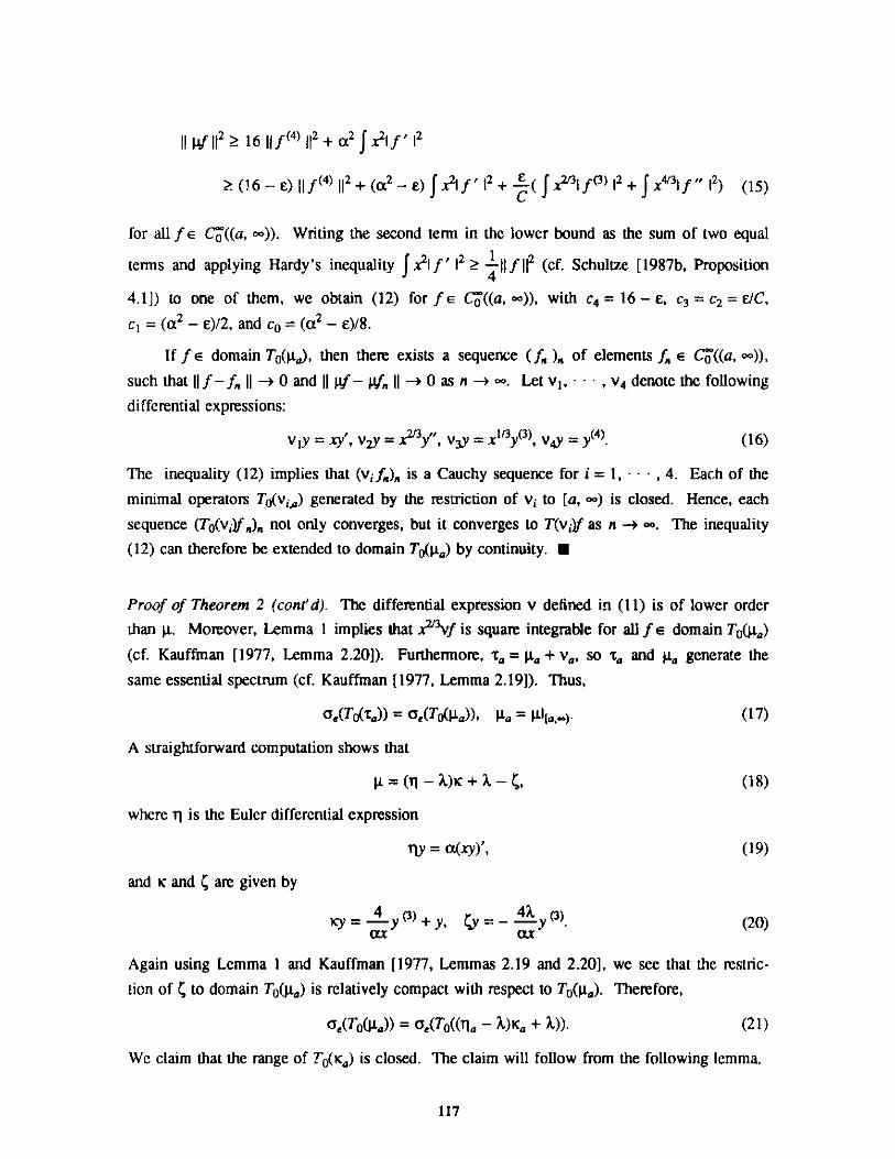
11 pf 12 16 11f 4, 112 + X2 jfX2 ,f'*12
(16 -E) ||f(4 02+ 2 - E) f 2 I2 + (X21I f(3)1|2+ 4 f."2) (15)
for all f e Co ((a, oo)). Writing the second term in the lower bound as the sum of two equal
terms and applying Hardy's inequality J x21 2f I1 If 112 (cf. Schultze [1987b, Proposition
4.1]) to one of them, we obtain (12) for f e Co((a, oo)), with c4 = 16 - e, c 3 = c2 = E/C,
cl = (a2 - e)/2, and Co = (a 2 - e)/8.
If f e domain T0(.ta), then there exists a sequence (fn ), of elements fn E Co ((a, oo)),
such that I1f -f, II -+ 0 and IIp p- pf,, II -+ 0 as n -+ o. Let v1 , , v4 denote the following
differential expressions:
v 1y = xy', v2y = xy,, v 3y = 1y )v 4 y(4). (16)
The inequality (12) implies that (v;f.), is a Cauchy sequence for i = 1, , 4. Each of the
minimal operators T0(v;,3) generated by the restriction of v; to [a, oo) is closed. Hence, each
sequence (To(v;)f.)n not only converges, but it converges to T(v;)f as n -+ oc. The inequality
(12) can therefore be extended to domain TT(Pa) by continuity. U
Proof of Theorem 2 (cont'd). The differential expression v defined in (11) is of lower order
than . Moreover, Lemma I implies that xnvf is square integrable for all f E domain T0 (pa)
(cf. Kauffman [1977, Lemma 2.20]). Furthermore, ta = a + Va, SO ta and pa generate the
same essential spectrum (cf. Kauffman [1977, Lemma 2.19]). Thus,
ae(TO(ta)) = ae(To(pa)), a = L[a,.). (17)
A straightforward computation shows that
p= (1 - X)K + 1 - (, (18)
where ,1 is the Euler differential expression
ny = a(xy)', (19)
and x and ( are given by
y = -y ( + y, Cy = - -y (. (20)ax ax
Again using Lemma I and Kauffman [1977, Lemmas 2.19 and 2.20], we see that the restric-
tion of C to domain T0 (Ja) is relatively compact with respect to T0 ( a). Therefore,
a,(T( a)) = ae(T((la - X)Ka + A)). (21)
We claim that the range of To(Ka) is closed. The claim will follow from the following lemma.
117
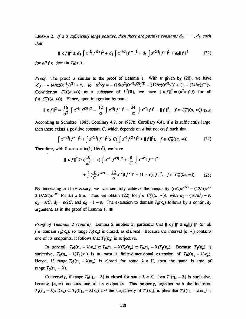
LEMMA 2. If a is suficiently large positive, then there are positive constants do, ' , d 3, such
that
II f|l2d 3 fx21f(3) 12+d2 Jx If" 2 +d1Jx-3 If' 2 +doIf1I 2 (22)
for allf E domain T0 (KC).
Proof The proof is similar to the proof of Lemma 1. With K given by (20), we have
S = - (4/ax-ly)(3) + y, so f y = - (16/ 2y(3 3) + (121a)(x-2 y')' + (1 + (24/Ax)x4)y.
Considering '((a, oo)) as a subspace of L2(R), we have II Kf 112 = (iKcif,f) for all
f E C '((a, co)). Hence, upon integration by parts,
II K fl| 2 = 16 fx-If()2 _ -J21f' 1 2 Jf 21f12 +|If|11 2 , f E Co ((a, )).(23)a2
According to Schultze 1985, Corollary 4.7, or 1987b, Corollary 4.4], if a is sufficiently large,
then there exists a pos dve constant C, which depends on a but not on f, such that
JX-413 f " ,2+ 1x~2-31f' 12 < C( x Y-2f(3 1 + 11 f112), f E Co((a, c ). (24)
Therefore, with 0 < E < min(1, 16/a2), we have
|| xf | 2 ( - ) x-12 + x |f "I
a2C
+ Jf(- -x~'1 - ai.x-2)I f ' 12 + (1 - E)II f 112, f E C ((a, c )). (25)
By increasing a if necessary, we can certainly achieve the inequality (E/C)x~r - (12/a)x-2
> (&'2C)x~21 for all x ? a. Thus we obtain (22) for f E C ((a, oo)), with d3 = (16/a2) - E,
d2 = E/C, dl = E/2C, and do = 1 - . The extension to domain T0(Ka) follows by a continuity
argument, as in the proof of Lemma 1. E
Proof of Theorem 2 (cont'd). Lemma 2 implies in particular that II Kf|112 ?doll f 12 for all
f e domain To(Ka), so range T0(Ka) is closed, as clairncd. Because the interval [a, oo) contains
one of its endpoints, it follows that Ti(Ka) is surjective.
In general, To((ma - X)Ka) c TO( - A)To(Ka) c T0 (Tj - X)T 1 (K,). Because T1(Oc) is
surjective, T0(T10 - X)Ti(lCa) is at most a finite-dimensional extension of To((11a - X)la).Hence, if range T((r - X)Ka) is closed for some A E C, then the same is true of
range T0 (fla - A).
Conversely, if range T0 (40 - X) is closed for some A E C, then T1(Th - X) is surjective,
because [a, oo) contains one of its endpoints. This property, together with the inclusion
Ti(fla - )T1(Ka) c Ti((fla - A)Ka) ar-1 the surjectivity of Ti(K 0), implies that T((rl - X)a) is
118
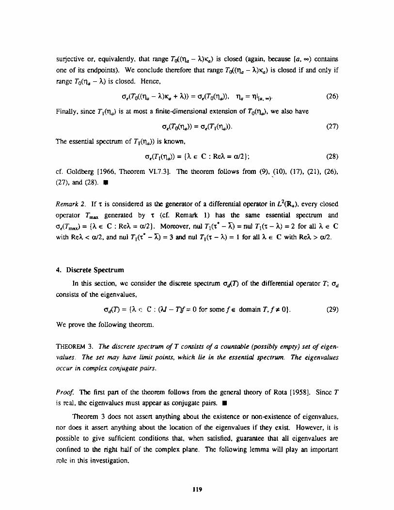
surective or, equivalently, that range T((na - X)K,) is closed (again, because [a, oo) contains
one of its endpoints). We conclude therefore that range T0 ((rla - .)Ka) is closed if and only if
range T0 (fla - X) is closed. Hence,
-(To((X - A)Ka + A)) = ae(To(Ti)), Tla = g1j.. (26)
Finally, since Ti(1,) is at most a finite-dimensional extension of To(a), we also have
a,(To(Tla)) = a,(T1(n.)). (27)
The essential spectrum of Ti(rla)) is known,
a,(T(g,)) = {A E C : Re? = ca2); (28)
cf. Goldberg [1966, Theorem VI.7.3]. The theorem follows from (9), (10), (17), (21), (26),
(27), and (28). U
Remark 2. If T is considered as the generator of a differential operator in L2 (R.), every closed
operator Tmx generated by r (cf. Remark 1) has the same essential spectrum and
ae(Tmn) = (aE C : ReX=/2). Moreover, nul Tl(t* - )= nul T(T - A) = 2 for all A.E C
with Re < ca2, and nul Ti(T* - X)= 3 and nul T1 c - A) = 1 for all A E C with Re > ca2.
4. Discrete Spectrum
In this section, we consider the discrete spectrum ad(T) of the differential operator T; ad
consists of the eigenvalues,
ad(7T) = { C : (Al - T)f = 0 for some f E domain T, f * 0). (29)
We prove the following theorem.
THEOREM 3. The discrete spectrum of T consists of a countable (possibly empty) set of eigen-
values. The set may have limit points, which lie in the essential spectrum. The eigenvalues
occur in complex conjugate pairs.
Proof The first part of the theorem follows from the general theory of Rota [1958]. Since T
is real, the eigenvalues must appear as conjugate pairs. U
Theorem 3 does not assert anything about the existence or non-existence of eigenvalues,
nor does it assert anything about the location of the eigenvalues if they exist. However, it is
possible to give sufficient conditions that, when satisfied, guarantee that all eigenvalues are
confined to the right half of the complex plane. The following lemma will play an important
role in this investigation.
119
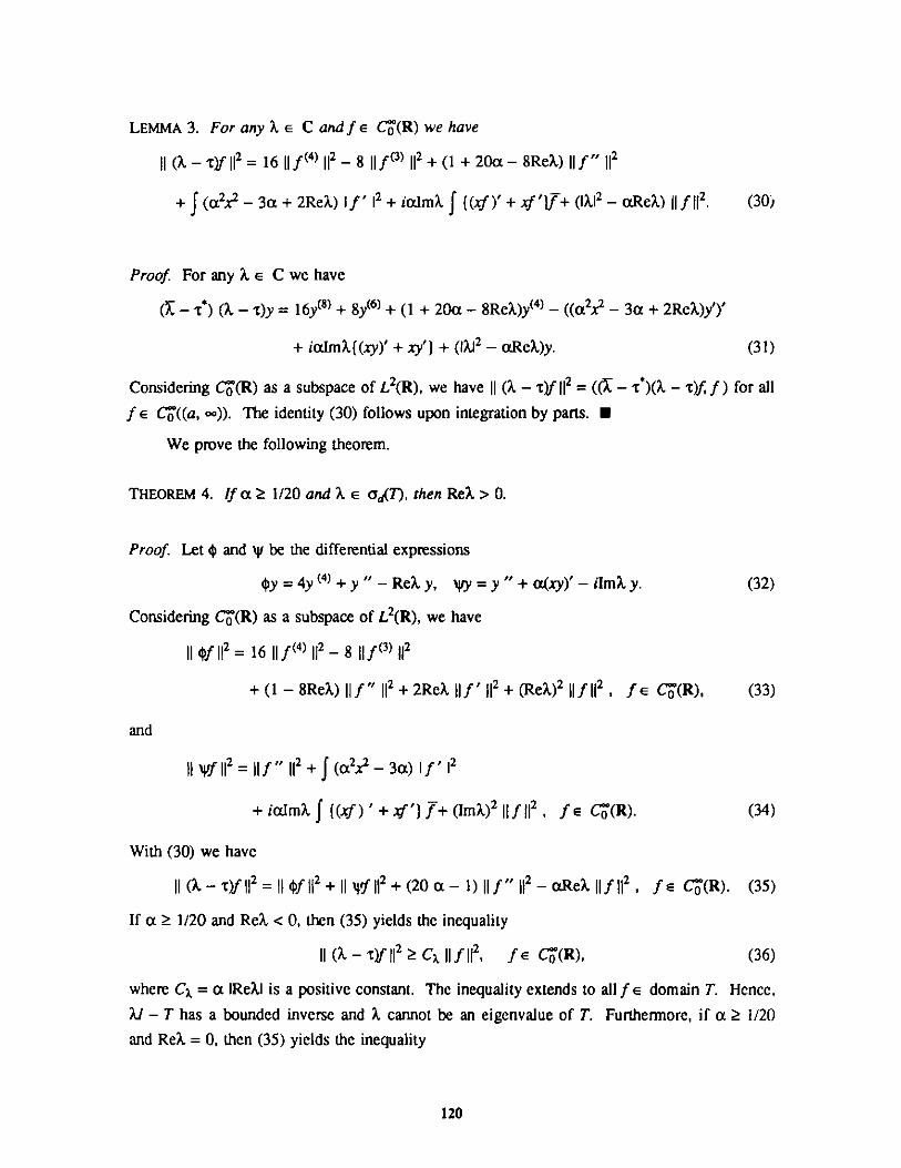
LEMMA 3. For any A. e C and f e Ca(R) we have
I (A - t)f 112 = 16 IIf 4) ||2 _ 8 If131 112 + (1 + 20a - 8ReX) |hf" 112
+ f (a 2x2 - 3a + 2ReX) I f ' 12 + ialmA J 4(xf)' + xf '}f+ (I1X 2 - aReX) If 112. (30)
Proof. For any A e C we have
(X - T*) (a - t)y = 16yt8 + 8y(6) + (1 + 20a - 8Re)y(4) - ((a 2x 2 - 3a + 2Re)y')'
+ ialm{(xy)' + xy') + (1X12 - aRe.)y. (31)
Considering Co(R) as a subspace of L2(R), we have II(A - t)f 112 =(( -*)(A - t)f, f) for all
f E Co ((a, oo)). The identity (30) follows upon integration by parts. U
We prove the following theorem.
THEOREM 4. If a z 1/20 and A e ad(T), then Re,> 0.
Proof. Let $ and yi be the differential expressions
$y=4y(4)+y"-Re y, y =y"+a(xy)'-im y. (32)
Considering C*(R) as a subspace of 13(R), we have
II $f 112 16 11f(4, 12- 8 hlff 3l 112
+ (1 - 8ReX) |hf " 112 + 2ReX |hf ' 112 + (ReX)2 l 2t 12, f e C(R), (33)
and
II Vft112 = If" 112 + J (a2x2 - 3a) If' 12
+ ialmA J (xf) ' + xf'} f+ (Im) 2 If112, fe C'(R). (34)
With (30) we have
II (A - t)f 112 =If11 2 + f 2 + (20 a - 1) |f" I2- -aReX |if 12, f¬E C(R). (35)
If a ? 1/20 and ReX < 0, then (35) yields the inequality
II (X - T)f112 ? C II112, f E C(R), (36)
where C, = a IReXI is a positive constant. The inequality extends to all f e domain T. Hence,
I - T has a bounded inverse and A cannot be an eigenvalue of T. Furthermore, if a 1/20
and ReX = 0, then (35) yields the inequality
120
II (? - 'r)f112 11 f 112, f e C(R). (37)
The inequality extends to all f E domain T. But if ReX = 0, then $y = 4y(4) + y", and the
equation $y = 0 has no solution in L2 (R) besides the trivial one. So we find again that ? can-not be an eigenvalue of T. U
The following theorem yields a sharper result for larger values of a.
THEOREM 5. If X e adT), then Rea , a/2 - 1/16.
Proof. Let x be the differential expression
1xy=2y" +-y. (38)
We have
| f12 4If" I2 _I' 112+ 1 11f11 2 0, fe Co(R). (39)
Therefore,
Re (Tf, f)= 4 |f "112- _ '1 2 |f11|2 a 16)112 , f E Co(R). (40)2 2 16
If ReX < - 6-, then it follows from Schwartz's inequality that
II(A-t)flII|fII Re((A-t1)ff) CI|fII2 , fe C(R), (41)
where C, = - - Rea is a positive constant. Hence, Al - T has a bounded inverse. U
The final theorem shows that the eigenvalues must lie to the left of the line Re = 9W8.
THEOREM 6. If X E ad(T), then Rey, < 9a/8.
Proof. The proof is similar to the proof of Theorem 4. Let $ and yi be the differential expres-
sions
$y=4y(4 )+y "+(-a-Re)y, iry=a(xy)'-lm y. (42)2
Considering Co(R) as a subspace of L2(R), we have
II $f112 = 16 If( 4) 112- 8 If(1)112 + (1 + 12a - 8ReX) hf" II2
+ (2Re - 3a)If'112 + (a - Re) 2 11f11 2 , fE C (R), (43)2
and
121
II f 112 = a 2 f x ,'|2
+ iocdmXJ {(xf) ' + x') f+ (ImX) 2 f11 2 , f e Co(R). (44)
With (30) we have
1 (I - t)f 112 -4f12 + i|ifl| + 8 a |hf" 112 + 2a(ReX - ia) If 112 , fe C6*(R). (45)8
If ReX > -ca, then (45) yields the inequality8
II (X - t)f112 > Ca .IIf 112, f E CO (R), (46)
where C% = 2a(ReX - -x) is a positive constant. The inequality extends to allif e domain T.8
Hence, XI - T has a bounded inverse and 7 cannot be an eigenvalue of T. Furthermore, if
Red = -a, then (45) yields the inequality8
II (X - t)f 112 8aIf" 112, f e Co(R). (47)
The inequality extends to all f e domain T. But the equation y" = 0 has no nontrivial solution
in L2 (R), so we find again that X cannot be an eigenvalue of T.
5. Conclusions
The fourth-order singular differential operator T defined in Section 2 has a non-empty
essential spectrum a,(7T) = (X e C: Rel = a/2) and a discrete spectrum ad(T), which consists
of countably many pairs of complex conjugate eigenvalues of T; ad(T) may be empty. The
eigenvalues are bounded on the left by the line ReX = a/2 - 1/16 and on the right by the line
ReX = 9a/8. If a 1/20, they are bounded on the left by the imaginary axis. The last resultimplies in particular that all separable solutions $ of (2) decay exponentially as t -+ oo if
a ? 1/20.
122
References
N. Dunford and J. Schwartz 1963. Linear Operators. Part II: Spectral Theory, Wiley, NewYork.
H. Frentzen 1987. "Limit-point criteria for not necessarily symmetric quasi-differential expres-sions," preprint.
S. Goldberg 1966. Unbounded Linear Operators, McGraw-Hill, New York.
R. M. Kauffman 1977. "On the limit-n classification of ordinary differential operators withpositive coefficients," Proc. London Math. Soc. 35, 496-526.
R. M. Kauffman, T. T. Read, and A. Zettl 1977. The Deficiency Index Problem for Powers ofOrdinary Differential Expressions, Lecture Notes in Mathematics 621, Springer-Verlag,New York.
D. Race 1985. "The theory of j-selfadjoint extensions of j-symmetric operators," J. Diff. Eq.!7, 258-274.
G. C. Rota 1958. "Extension theory of differential operators," Comm. Pure Appl. Math. 11,23-65.
B. Schultze 1983. "A limit-point criterion for even-order symmetric differential expressionswith positive supporting coefficients," Proc. London Math. Soc. (3) 46, 561-576.
B. Schultze 1985. "Ordinary differential expressions with positive supporting coefficients,"Habilitationsschrift.
B. Schultze 1987a. "On the essential spectrum of linear ordinary differential expressions,"prprint.
B. Schultze 1987b. "Odd-order ordinary differential expressions with positive supportingcoefficients," Proc. Roy. Soc. Edinburgh 105A, 167-192.
G. I. Sivashinsky, C. K. Law, and G. Joulin 1982. "On stability of premixed flames instagnation-point flow," Combustion Science and Technol. 28, 155-159.
123
SINGULAR SELF-ADJOINT STURM-LIOUVILLE PROBLEMS, I:A SIMPLE APPROACH TO THE PROBLEM WITH SINGULAR ENDPOINTS
A. M. KralDepartment of Mathematics
Pennsylvania State UniversityUniversity Park, PA 16802
A. Zett(Department of MathematicsNorthern Illinois University
DeKalb, IL 60115
Abstract
Singular self-adjoint boundary conditions for Sturm-Liouville problems arecharacterized. We believe this characterization is new, simpler, and moreexplicit than the well-known characterization and an exact parallel of the regu-lar case.
1. Introduction
There are two fundamental classes of boundary value problems for the Sturm-Liouville
expression
My = -[-(py')'+qy] on I = (a,b), -00 a < b 0, (1.1)w
i.e., regular and singular. In both cases the boundary conditions required to obtain self-adjoint
realizations of M are well known (and have been known for over a century). For details see
the book by Naimark [1968]. In the regular case these conditions can be interpreted as linear
combinations of the values of the function y and its quasi-derivative py' at the end points a and
b. Such a representation is not possible at a singular endpoint c, say, because y(c) and (py')(c)
do not exist even in a limiting sense, in general. The known characterization of the singular
self-adjoint boundary conditions involves the sesquilinear form associated with M and elements
of the maximal domain. In this paper we show that the characterization of the singular self-
adjoint boundary conditions is identical to that in the regular case provided that y and py' are
replaced by certain Wronskians involving y and two linearly independent solutions of My = 0.
Participant in Faculty Research Leave at Argonne program, Mathematics and Computer Science Division,Argonne National Laboratory, September 1986 - June 1987.
/41/ 125
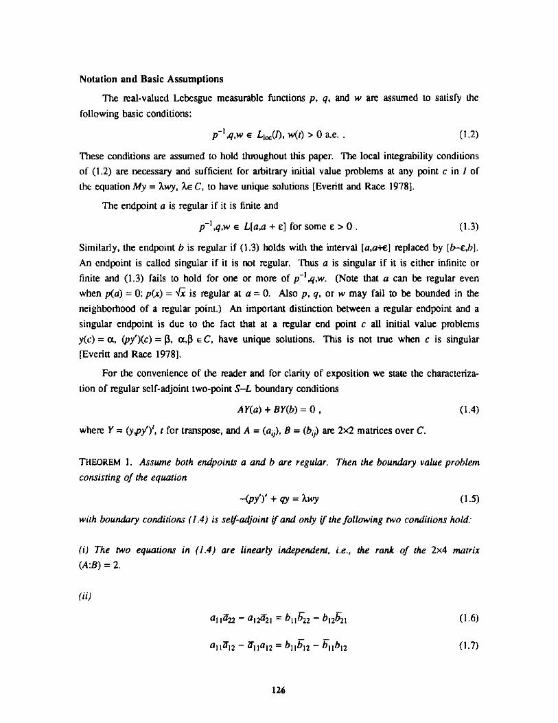
Notation and Basic Assumptions
The real-valued Lebesgue measurable functions p, q, and w are assumed to satisfy the
following basic conditions:
p-1,q,w E L1i(b), w(t) > 0 a.e. . (1.2)
These conditions are assumed to hold throughout this paper. The local integrability conditions
of (1.2) are necessary and sufficient for arbitrary initial value problems at any point c in 1 of
the equation My = Xwy, Xe C, to have unique solutions [Everitt and Race 1978].
The endpoint a is regular if it is finite and
p-1,q,w e L[a,a + el for some e > 0 . (1.3)
Similarly, the endpoint b is regular if (1.3) holds with the interval [a,a+E] replaced by [b-E,b].
An endpoint is called singular if it is not regular. Thus a is singular if it is either infinite or
finite and (1.3) fails to hold for one or more of p~1 q,w. (Note that a can be regular even
when p(a) = 0: p(x) = V6 is regular at a = 0. Also p, q, or w may fail to be bounded in the
neighborhood of a regular point.) An important distinction between a regular endpoint and a
singular endpoint is due to the fact that at a regular end point c all initial value problems
y(c) = a, (py')(c)= P, a,$ e C, have unique solutions. This is not true when c is singular
[Everitt and Race 1978].
For the convenience of the reader and for clarity of exposition we state the characteriza-
tion of regular self-adjoint two-point S-L boundary conditions
AY(a) + BY(b) = 0 , (1.4)
where Y = (y,py')', t for transpose, and A = (a,), B = (bid) are 2x2 matrices over C.
THEOREM 1. Assume both endpoints a and b are regular. Then the boundary value problem
consisting of the equation
-(py')' + qy = ?wy (1.5)
with boundary conditions (1.4) is self-adjoint if and only if the following two conditions hold:
(i) The two equations in (1.4) are linearly independent, i.e., the rank of the 2x4 matrix
(A:B) = 2.
(ii)
a 11 22 - a12a21 = b11b2 2 - b12b2 1 (1.6)
a, 1 12 - 11a1 2 = b11b12 - b11b12 (1.7)
126
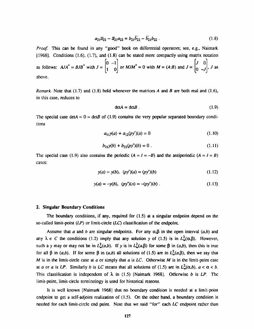
a21a22 - a21a 22 = b21622 - b2 b2 (
Proof. This can be found in any "good" book on differential operators; see, e.g., Naimark
[1968]. Conditions (1.6), (1.7), and (1.8) can be stated more compactly using matrix notation
as follows: AJA* = BJB* withJ= 01 0 orMJM = 0 with M = (A:B) and J=0 -J , J as
above.
Remark. Note that (1.7) and (1.8) hold whenever the matrices A and B are both real and (1.6),
in this case, reduces to
detA = detB . (1.9)
The special case detA = 0 = detB of (1.9) contains the very popular separated boundary condi-
tions
a11 y(a) + a1 2(py')(a) = 0 (1.10)
b21y(b) + b22 (py')(b) = 0 . (1.11)
The special case (1.9) also contains the periodic (A = I = -B) and the antiperiodic (A = 1 = B)
cases:
y(a) = y(b), (py')(a) = (py')(b) (1.12)
y(a) = -y(b), (py')(a) = -(py')(b) . (1.13)
2. Singular Boundary Conditions
The boundary conditions, if any, required for (1.5) at a singular endpoint depend on the
so-called limit-point (LP) or limit-circle (LC) classification of the endpoint.
Assume that a and b are singular endpoints. For any a,$ in the open interval (a,b) and
any A E C the conditions (1.2) imply that any solution y of (1.5) is in L ,(a,). However,
such a y may or may not be in L,(a,b). If y is in Lj(a,4) for some $ in (a,b), then this is true
for all p in (a,b). If for some $ in (a,b) all solutions of (1.5) are in L(a,), then we say that
M is in the limit-circle case at a or simply that a is LC. Otherwise M is in the limit-point case
at a or a is LP. Similarly b is LC means that all solutions of (1.5) are in L(a,b), a < a < b.
This classification is independent of A in (1.5) [Naimark 1968]. Otherwise b is LP. The
limit-point, limit-circle terminology is used for historical reasons.
It is well known [Naimark 1968] that no boundary condition is needed at a limit-point
endpoint to get a self-adjoint realization of (1.5). On the other hand, a boundary condition is
needed for each limit-circle end point. Note that we said "for" each LC endpoint rather than
127
(1. 8)
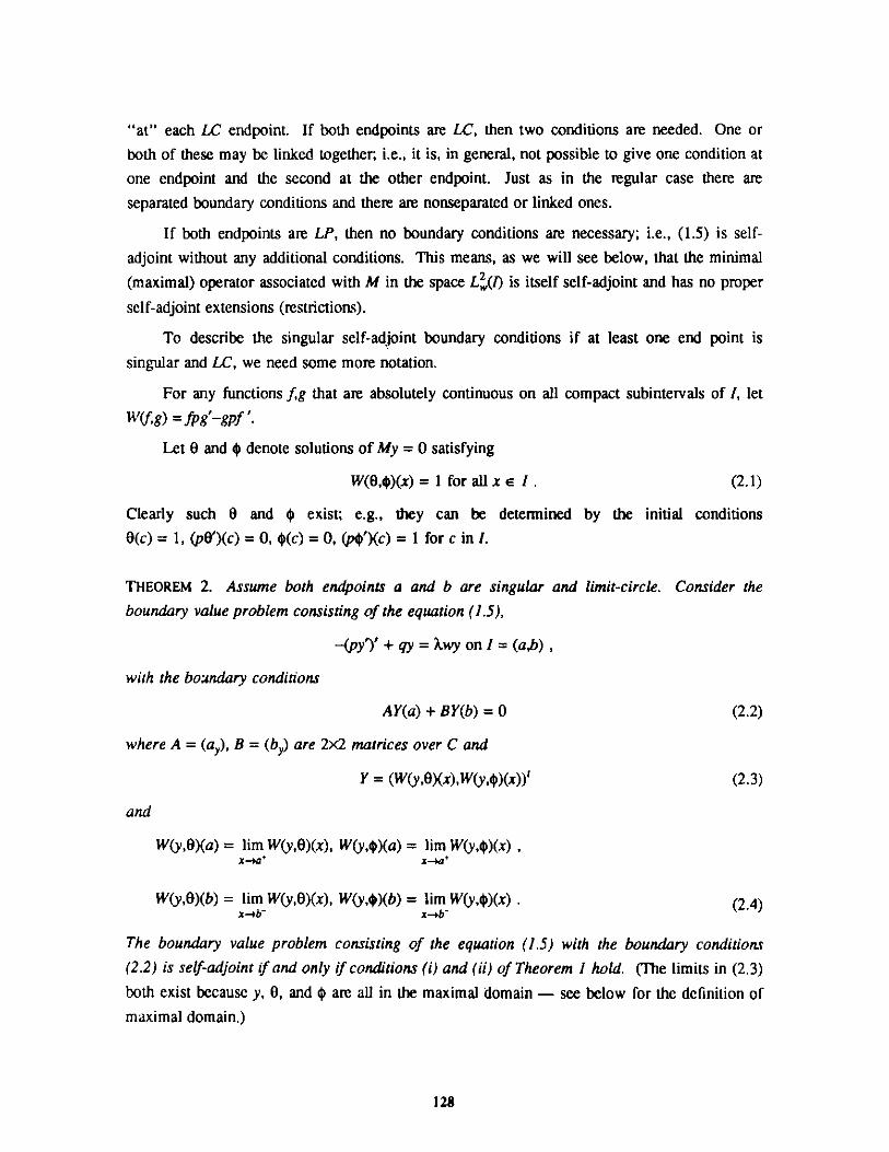
"at" each LC endpoint. If both endpoints are LC, then two conditions are needed. One or
both of these may be linked together; i.e., it is, in general, not possible to give one condition at
one endpoint and the second at the other endpoint. Just as in the regular case there are
separated boundary conditions and there are nonseparated or linked ones.
If both endpoints are LP, then no boundary conditions are necessary; i.e., (1.5) is self-
adjoint without any additional conditions. This means, as we will see below, that the minimal
(maximal) operator associated with M in the space L%(l) is itself self-adjoint and has no proper
self-adjoint extensions (restrictions).
To describe the singular self-adjoint boundary conditions if at least one end point is
singular and LC, we need some more notation.
For any functions f,g that are absolutely continuous on all compact subintervals of I, let
W(fg) =fpg'-gpf'.
Let 0 and 4) denote solutions of My = 0 satisfying
W(0,4))(x) = 1 for all xE I. (2.1)
Clearly such 0 and 4) exist; e.g., they can be determined by the initial conditions
0(c) = 1, (pO')(c) = 0, 4)(c) = 0, (p$'Xc) = 1 for c in 1.
THEOREM 2. Assume both endpoints a and b are singular and limit-circle. Consider the
boundary value problem consisting of the equation (1.5),
-(py')' + qy = Xwy on I = (a,b),
with the boundary conditions
AY(a) + BY(b) = 0 (2.2)
where A = (a), B = (by) are 2x2 matrices over C and
Y = (W(y,0)(x),W(y,4))(x))' (2.3)
and
W(y,0)(a) = lim W(y,0)(x), W(y,4))(a) = lim W(y,4))(x) ,x-a t
x-+a +
W(y,0)(b) = lim W(y,0)(x), W(y,$)(b) = lim W(y,4))(x) . (2.4)
The boundary value problem consisting of the equation (1.5) with the boundary conditions
(2.2) is self-adjoint if and only if conditions (i) and (ii) of Theorem 1 hold. (The limits in (2.3)
both exist because y, 0, and $ are all in the maximal domain - see below for the definition of
maximal domain.)
128
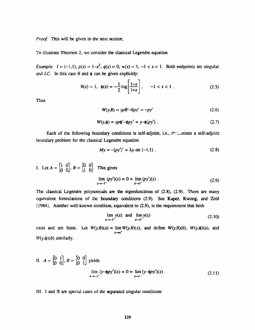
Proof. This will be given in the next section.
To illustrate Theorem 2, we consider the classical Legendre equation.
Example. 1 = (-1,1), p(x) = 1-x2, q(x) = 0, w(x) = 1, -1 < x < 1. Both endpoints are singular
and LC. In this case 0 and $ can be given explicitly:
Thus
W(y,0) = yp0'-Opy' = -py' (2.6)
W(y,$) = yp4)'-4py' = y-(py'). (2.7)
Each of the following boundary conditions is self-adjoint, i.e., &'.,nines a self-adjoint
boundary problem for the classical Legendre equation
My = -(py')' = Xy on (-1,1) . (2.8)
1. Let A = 11 0, B =00 . This gives
lim (py'Xx) = 0 = lim (py')(x) . (2.9)x-+-1 +x-+
The classical Legendre polynomials are the eigenfunctions of (2.8), (2.9). There are many
equivalent formulations of the boundary conditions (2.9). See Kaper, Kwong, and Zettl
[1984]. Another well-known condition, equivalent to (2.9), is the requirement that both
lim y(x) and limy(x) (2.10)x-+,-1+ x-1-
exist and are finite. Let W(y,0)(a) = lim W(y,0)(x), and define W(y,0)(b), W(y,4)(a), andX-+a*
W(y,4)(b) similarly.
II. A = 1 B [= yieldsslim (y-$py')(x) = 0 = lim (y-py')(x) . (2.11)
x-+-14 x-+1~
III. I and II are special cases of the separated singular conditions
129
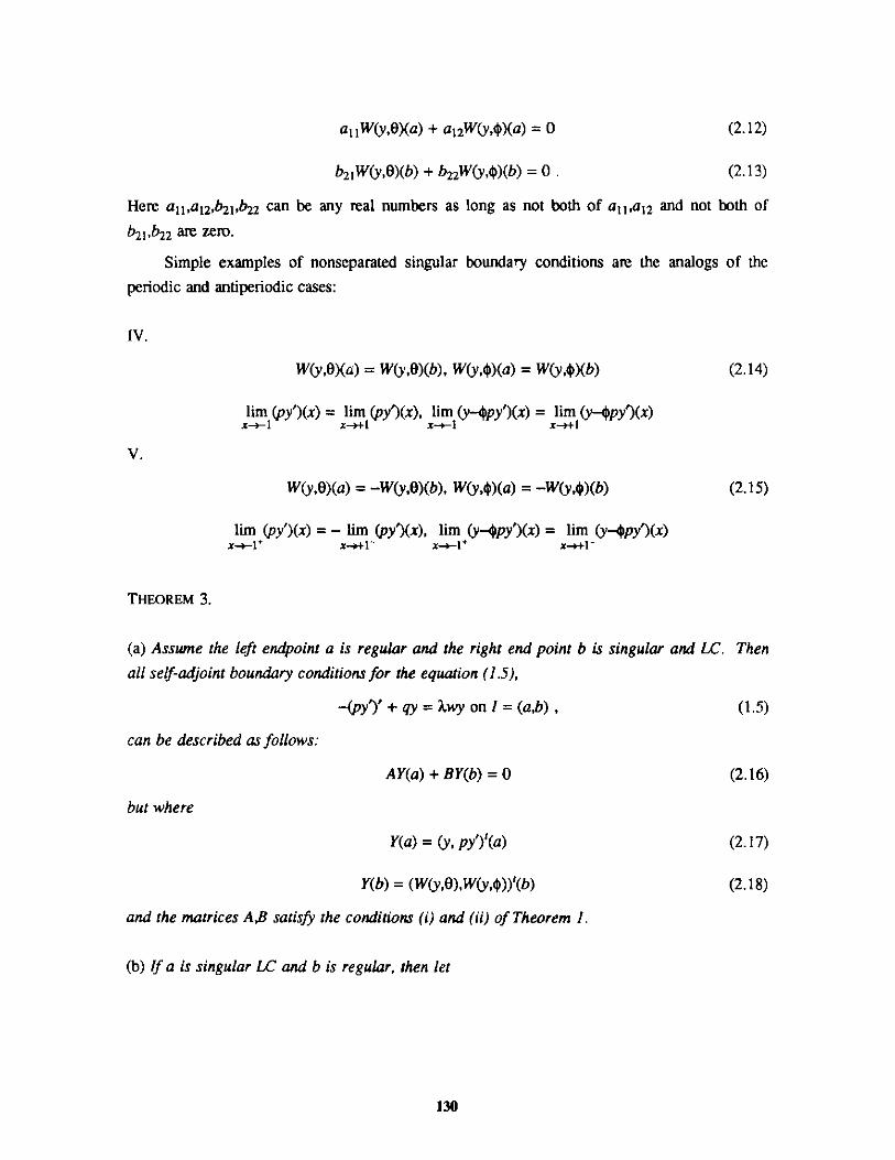
a, W(y,0)(a) + al2W(y,$)(a) = 0
b2 1W(ye)(b) + b22W(y,$)(b) = 0.
(2.12)
(2.13)
Here a11,a 12 ,b2 1,b22 can be any real numbers as long as not both of a11,a12 and not both of
b21,b22 are zero.
Simple examples of nonseparated singular boundary conditions are the analogs of the
periodic and antiperiodic cases:
IV.
W(y,O)(a) = W(yO)(b), W(y,$)(a) = W(y,$)(b)
V.
(2.14)
lim (py')(x) = lim (py')(x), lim (y-4py')(x) = lim (y-4py')(x)x-+-1 x-++1 x-+- z-++1
W(y,O)(a) = -W(y,O)(b), W(y,$)(a) = -W(y,$)(b)
lim (py')(x) = - lim (py')(x), lim (y-4py')(x) = lim (y-4py')(x)
(2.15)
THEOREM 3.
(a) Assume the left endpoint a is regular and the right end point b is singular and LC. Then
all self-adjoint boundary conditions for the equation (1.5),
-(py')' + qy = Xwy on 1 = (a,b) ,
can be described as follows:
but where
AY(a) + BY(b) = 0
Y(a) = (y, py')'(a)
(1.5)
(2.16)
(2.17)
(2.18)Y(b) = (W(yO),W(y,$))'(b)
and the matrices A,B satisfy the conditions (i) and (ii) of Theorem 1.
(b) If a is singular LC and b is regular, then let
130
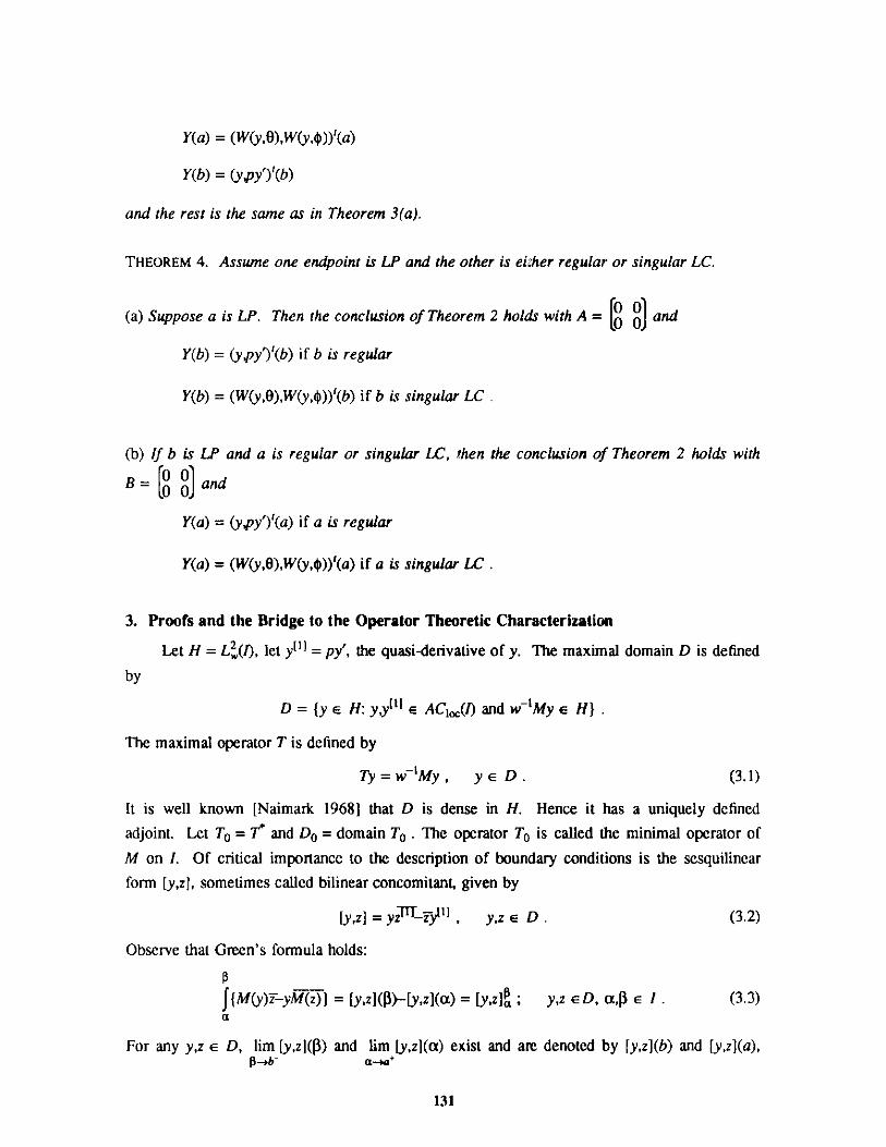
Y(a) = (W(y,O),W(y,$))(a)
Y(b) = (ypy')'(b)
and the rest is the same as in Theorem 3(a).
THEOREM 4. Assume one endpoint is LP and the other is either regular or singular LC.
(a) Suppose a is LP. Then the conclusion of Theorem 2 holds with A = [0 0])and
Y(b) = (y py')'(b) if b is regular
Y(b) = (W(y,0),W(y,4))'(b) if b is singular LC .
(b) If b is LP and a is regular or singular LC, then the conclusion of Theorem 2 holds with
B = [ and
Y(a) = (y py')'(a) if a is regular
Y(a) = (W(y,0),W(y,$))'(a) if a is singular LC .
3. Proofs and the Bridge to the Operator Theoretic Characterization
Let H = Lw(I), let y[IJ = py', the quasi-derivative of y. The maximal domain D is defined
by
D = {y e H: y,yU[I e AC1,(f) and w~1My e H)
The maximal operator T is defined by
Ty =w~1My, ye D. (3.1)
It is well known [Naimark 1968] that D is dense in H. Hence it has a uniquely defined
adjoint. Let To = T* and Do = domain To0. The operator To is called the minimal operator of
M on 1. Of critical importance to the description of boundary conditions is the sesquilinear
form [y,z], sometimes called bilinear concomitant, given by
[y,z] = yzTlT-yIJ , y,z E D . (3.2)
Observe that Green's formula holds:
f(M(y)a-yM(z)) = [y,z]($)-[y,z](a) = [y,z], ; y,z ED, a4 e 1. (3.3)
For any y,z e D, lim [y,z](p) and lim [y,z](a) exist and are denoted by [y,z](b) and [y,z](a),%->b-a-+a +
131
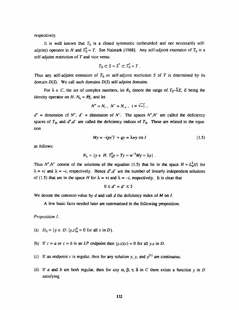
respectively.
It is well known that To is a closed symmetric (unbounded and not necessarily self-
adjoint) operator in H and T = T. See Naimark [1968]. Any self-adjoint extension of To is a
self-adjoint restriction of T and vice versa:
To c S =S c = T.
Thus any self-adjoint extension of To or self-adjoint restriction S of T is determined by its
domain D(S). We call such domains D(S) self-adjoint domains.
For A e C, the set of complex numbers, let RX denote the range of To-4E, E being the
identity operator on H; N = R{, and let
N=N;, N~=N_, i= ,
d+ = dimension of N*, d~ = dimension of N. The spaces N,N are called the deficiency
spaces of To, and d,d- are called the deficiency indices of To. These are related to the equa-
tion
My = -(py')' + qy = Xwy on!1 (1.5)
as follows:
NX = {ye H: Ty =Ty=w'My=ky).
Thus N,N~ consist of the solutions of the equation (1.5) that lie in the space H = Lw,() for
a = +i and ? = -i, respectively. Hence d,d~ are the number of linearly independent solutions
of (1.5) that are in the space H for X = +i and X = -i, respectively. It is clear that
0 5d' =d-< 2 .
We denote the common value by d and call d the deficiency index of M on I.
A few basic facts needed later are summarized in the following proposition.
Proposition 1.
(a) Do0 = {y e D: [y,z]= 0 for all z in D).
(b) Ifc=aorc=b is an LP endpoint then [y,z](c) = 0 for all y,zinD.
(c) If an endpoint c is regular, then for any solution y, y, and y[1 are continuous.
(d) If a and b are both regular, then for any a, a, y, S in C there exists a function y in D
satisfying
132
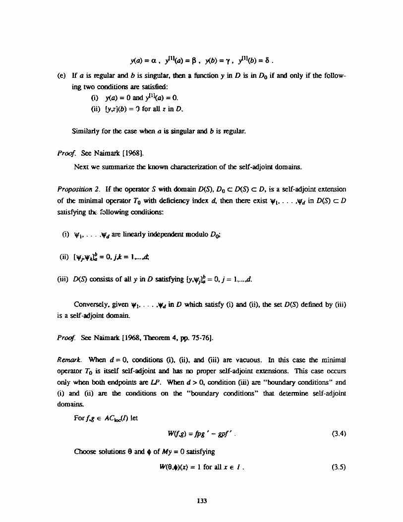
(e) If a is regular and b is singular, then a function y in D is in Do if and only if the follow-
ing two conditions are satisfied:
(i) y(a)=0andy1(a)=0.
(ii) [y,z](b) = ) for all z in D.
Similarly for the case when a is singular and b is regular.
Proof. See Naimark [1968].
Next we summarize the known characterization of the self-adjoint domains.
Proposition 2. If the operator S with domain D(S), Do c D(S) c D, is a self-adjoint extension
of themoporTTw ihdefi indexdthen thereexist 'I, ... ,ysdin D(S) c D
satisfying tht. following conditions:
(i) WI, ... ,Vd are linearly independent modulo Da;
(ii) [ykJ = 0, j,k = 1,...4
(iii) D(S) consists of all y in D satisfying [y,yi]Q= 0, j = l,...,.
Conversely, given y, ... ,yd in D which satisfy (i) and (i), the set D(S) defined by (iii)
is a self-adjoint domain.
Proof. See Naimark [1968, Theorem 4, pp. 75-76].
Remark. When d = 0, conditions (7), (ii), and (iii) are vacuous. In this case the minimal
operator To is itself self-adjoint and has no proper self-adjoint extensions. This case occurs
only when both endpoints are LP. When d > 0, condition (iii) are "boundary conditions" and
(i) and (ii) are the conditions on the "boundary conditions" that determine self-adjoint
domains.
Forf,g E AC Jc(I) let
W(fg)=fpg' - gpf' . (3.4)
Choose solutions 0 and $ of My = 0 satisfying
W(0,$Xx) = 1 for allx e 1. (3.5)
133
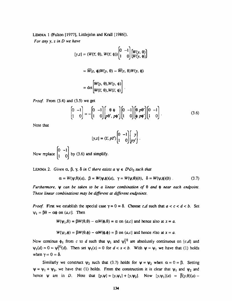
LEMMA 1 (Fulton [1977], Littlejohn and Krall [1986]).
For any y, z in D we have
[y,z] = (W(-, 0), W(- $],)) - ]
= W(z, $)W(y, 0) - W(z, 0)W(y, $)
W(y, O),W(y, )= det W(, 0),W(, 4)J
Proof. From (3.4) and (3.5) we get
0 -1 0 -1 00$ 0 -1 a pe' 0 -1
1 0 1 0 L.', p$' 1 0 $ p$' 1 0 '36
Note that
o -1 1y[y'z] = (, P=') 1 0 py'
0 -1Now replace 1 0 by (3.6) and simplify.
LEMMA 2. Givenay,8in C there exists a yVE D\D0 such that
a = W(y4,)(a), 3 = W(1,$)(a), y = W(i,8)(b), 8 = W(4,4)(b) . (3.7)
Furthermore, i can be taken to be a linear combination of 0 and $ near each endpoint.
These linear combinations may be different at different endpoints.
Proof. First we establish the special case y = 0 = 8. Choose c,d such that a < c < d < b. Set
= - c4 on (a,c]. Then
W(y 1,0) = 1W(0,0) - aW(,0) = a on (a,c] and hence also at x = a.
W(y1,)= 3W(0,$) - aW($,$) = $ on (a,c] and hence also at x = a.
Now continue $1 from c to d such that y1 and ir4'l are absolutely continuous on [c,d] and
yl(d) = 0 = j411(d). Then set W,(x) = 0 for d < x < b. With yi = yi we have that (1) holds
when y = 0 = S.
Similarly we construct y'2 such that (3.7) holds for W = '42 when a = 0 = . Setting
y' = 'i + y2, we have that (1) holds. From the construction it is clear that 4i and y2 andhence 4r are in D. Note that [yi] = [Y,'41i] + [y,'2]. Now [y,y 1](a) = 0[y,0](a) -
134
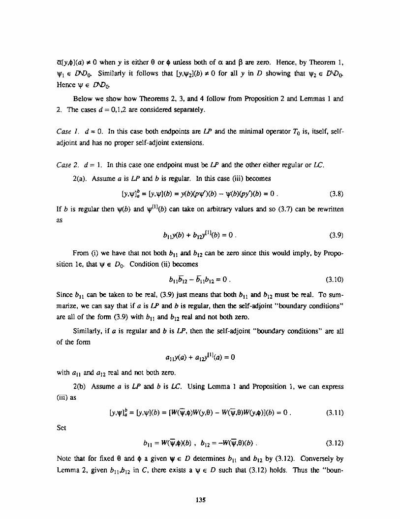
U[y,$](a) * 0 when y is either 0 or $ unless both of a and $ are zero. Hence, by Theorem 1,
V1 e DAD0. Similarly it follows that [y,yi 2 ](b) * 0 for all y in D showing that y'2 E D\D0 .Hence e LADO.
Below we show how Theorems 2, 3, and 4 follow from Proposition 2 and Lemmas 1 and
2. The cases d = 0,1,2 are considered separately.
Case 1. d = 0. In this case both endpoints are LP and the minimal operator To is, itself, self-
adjoint and has no proper self-adjoint extensions.
Case 2. d = 1. In this case one endpoint must be LP and the other either regular or LC.
2(a). Assume a is LP and b is regular. In this case (iii) becomes
[y,W] = [y,y](b) = y(b)(p')(b) - y(b)(py')(b) = 0 . (3.8)
If b is regular then y(b) and Wi 1 (b) can take on arbitrary values and so (3.7) can be rewrittenas
b11y(b) + b12y' 1 (b) = 0 . (3.9)
From (i) we have that not both b11 and b12 can be zero since this would imply, by Propo-
sition le, that yi E Do. Condition (ii) becomes
b11b12 - b11b12 = 0 . (3.10)
Since b11 can be taken to be real, (3.9) just means that both b11 and b12 must be real. To sum-
marize, we can say that if a is LP and b is regular, then the self-adjoint "boundary conditions"
are all of the form (3.9) with b11 and b12 real and not both zero.
Similarly, if a is regular and b is LP, then the self-adjoint "boundary conditions" are all
of the form
a11y(a) + ai 2y!(a) = 0
with all and a12 real and not both zero.
2(b) Assume a is LP and b is LC. Using Lemma 1 and Proposition 1, we can express
(iii) as
[y,wia = [y,y](b) = [W(4,$)W(y,6) - W(14,0)W(y,$)](b) = 0 . (3.11)
Set
bll = W(,$)Xb) , b12 = -W(5y,0)(b) . (3.12)
Note that for fixed 0 and $ a given yr e D determines b11 and b12 by (3.12). Conversely by
Lemma 2, given b11,b12 in C, there exists a yi E D such that (3.12) holds. Thus the "boun-
135
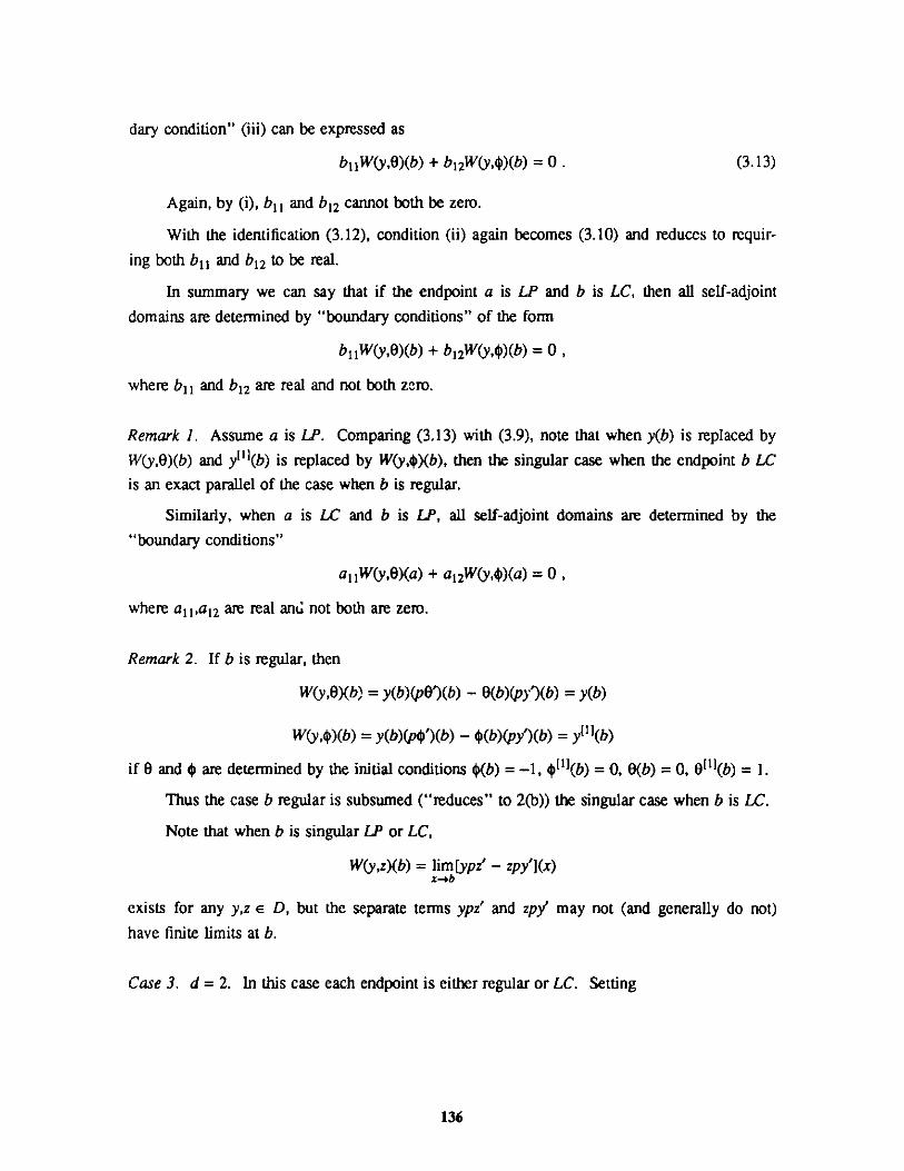
dary condition" (iii) can be expressed as
b11W(y,0)(b) + b12W(y,4)(b) = 0 . (3.13)
Again, by (i), b11 and b12 cannot both be zero.
With the identification (3.12), condition (ii) again becomes (3.10) and reduces to requir-
ing both b1 1 and b12 to be real.
In summary we can say that if the endpoint a is LP and b is LC, then all self-adjoint
domains are determined by "boundary conditions" of the form
b11W(y,0)(b) + b12W(y,$)(b) = 0,
where b11 and b12 are real and not both zero.
Remark 1. Assume a is LP. Comparing (3.13) with (3.9), note that when y(b) is replaced by
W(y,0)(b) and y~l1 (b) is replaced by W(y,$)(b), then the singular case when the endpoint b LC
is an exact parallel of the case when b is regular.
Similarly, when a is LC and b is LP, all self-adjoint domains are determined by the
"boundary conditions"
a11 W(y,0)(a) + a1 2W(y,$)(a) = 0 ,
where a11,a12 are real and not both are zero.
Remark 2. If b is regular, then
W(y,0)(b) = y(b)(pO')(b) - 0(b)(py')(b) = y(b)
W(y,4)(b) = y(b)(p$')(b) - $(b)(py')(b) = y'11(b)
if 0 and $ are determined by the initial conditions 4(b) = -1, 111(b) = 0, 0(b) = 0, 0'1(b) = 1.
Thus the case b regular is subsumed ("reduces" to 2(b)) the singular case when b is LC.
Note that when b is singular LP or LC,
W(y,zXb) = lim[ypz' - zpy'](x)x-+b
exists for any y,z e D, but the separate terms ypz' and zpy' may not (and generally do not)
have finite limits at b.
Case 3. d = 2. In this case each endpoint is either regular or LC. Setting
136
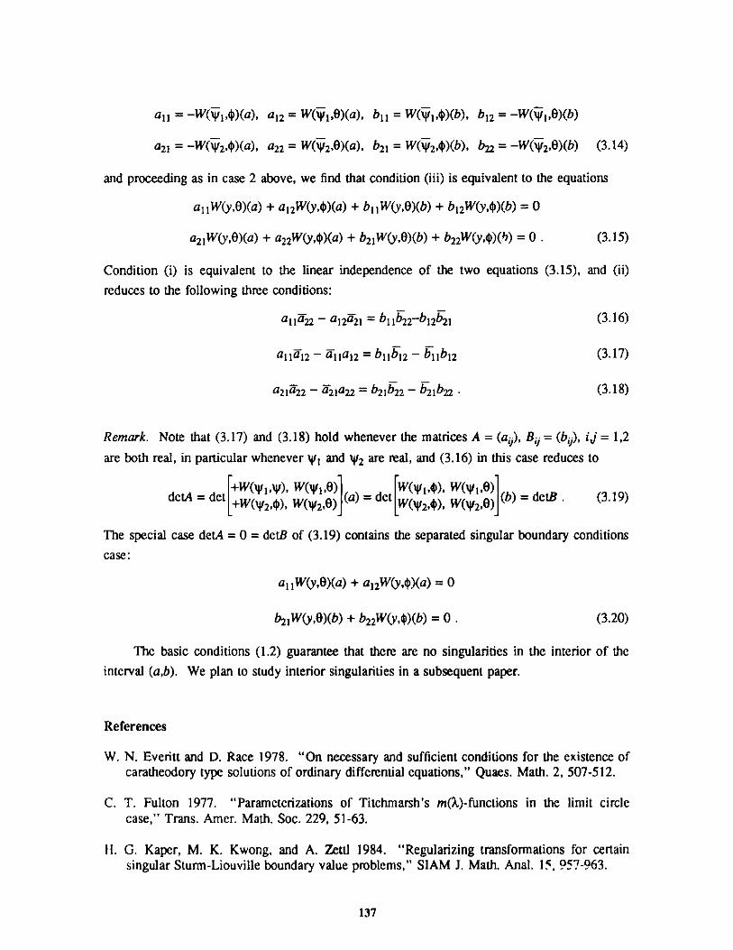
all = -W(iy 1 ,$)(a), a12 = W(1,4)(a), b11 = W( 1 ,4)(b), b12 = -W(i,6)(b)
a21 = -W(w2,4)(a), a22 = W(y 2 ,O)(a), b21 = W(N 2 ,4)(b), b2 = -W('y 2 ,6)(b) (3.14)
and proceeding as in case 2 above, we find that condition (iii) is equivalent to the equations
al 1W(y,0)(a) + a12W(y,4)(a) + b1 1 W(y,O)(b) + b12W(y,$)(b) = 0
a21W(y,O)(a) + a22W(y,$)(a) + b21W(y,O)(b) + b22W(y,4)(h) = 0 . (3.15)
Condition (i) is equivalent to the linear independence of the two equations (3.15), and (ii)reduces to the following three conditions:
a ia - a12 21 = b1b2-b12b21 (3.16)
a112 - 11 a1 2 =bbl2 - bllbl2 (3.17)
a21a2 - 21a2 2 = b21b2 - b 2 1b22 . (3.18)
Remark. Note that (3.17) and (3.18) hold whenever the matrices A = (aid), By = (b), i jJ= 1,2
are both real, in particular whenever y, and yN2 are real, and (3.16) in this case reduces to
det = et+W(4 i,y), W(yvlO)1)=de W(i,$~), W(141,O)1detA = det +W(V2,$), W(i 2,O)](a) = det W(2,), W( 42,)J(b) = detB . (3.19)
The special case detA = 0 = detB of (3.19) contains the separated singular boundary conditions
case:
a11 W(y,O)(a) + a1 2W(y,4)(a) = 0
b21W(y,O)(b) + b22 W(y,4)(b) = 0 . (3.20)
The basic conditions (1.2) guarantee that there are no singularities in the interior of the
interval (a,b). We plan to study interior singularities in a subsequent paper.
References
W. N. Everitt and D. Race 1978. "On necessary and sufficient conditions for the existence ofcaratheodory type solutions of ordinary differential equations," Quaes. Math. 2, 507-512.
C. T. Fulton 1977. "Parameterizations of Titchmarsh's m(X)-functions in the limit circlecase," Trans. Amer. Math. Soc. 229, 51-63.
1H. G. Kaper, M. K. Kwong, and A. Zettl 1984. "Regularizing transformations for certainsingular Sturm-Liouville boundary value problems," SIAM J. Math. Anal. 15, 957-963.
137
L. L. Littlejohn and A. M. Krall 1986. "Orthogonal polynomials and singular Sturm-Liouvillesystems," Rocky Mt. J. Math. 16, 435-479.
M. A. Naimark 1968. Linear Differential Operators: II, Ungar, New York.
SINGULAR SELF-ADJOINT STURM-LIOUVILLE PROBLEMS, II:INTERIOR SINGULAR POINTS
A. M. KralDepartment of Mathematics
Pennsylvania State UniversityUniversity Park, PA 16802
A. Zettl*Department of MathematicsNorthern Illinois University
DeKalb, IL 60115
Abstract
We consider the second-order Sturm-Liouville operator
ly = [-(py) + qy]/w
over a region (a,b) on the real line, -- a < b 5 oo, on which the operatormay have a finite number of singular points. By considering I over varioussubintervals on which singularities occur only at the ends, restrictions of themaximal operator generated by I in L(a,b) may be found which are self-adjoint. In addition to direct sums of self-adjoint operators defined on theseparate subintervals, there are other self-adjoint restrictions of the maximaloperator that involve linking the various intervals in interface-like style.
1. Introduction
This article is an extension of the work of W. N. Everitt and A. Zettl [1986], which dealt
with the problem of finding self-adjoint operators of the form
ly = [-py')' + qy]/w
with one interior singular point, or possibly over two disjoint intervals, using singular Naimark
boundary forms [Naimark 1967]. We use the equivalent concrete boundary representation dis-
cussed by Krall and Zettl [1988] and consider finitely many singular points, or perhaps finitely
many disjoint intervals.
The extension to many singular points or many disjoint intervals is done with relative
ease because we use the explicit Fulton-type boundary forms exhibited in [Fulton 1977; Krall
and Zettl 1988; Littlejohn and Krall 1986a] for singular ends. By using these concrete forms,
not only are direct sum self-adjoint operators easily exhibited, but also self-adjoint operators
whose boundaries are linked together are explicitly described. We also bypass the abstract and
Participant in Faculty Research Leave at Argonne program, MrThematics and Computer ScienceDivision, Argonne National Laboratory, September 1986 - June 1987.
3/ 139
rather difficult-to-use Naimark boundary forms found in [Naimark 1967].
We assume that the terminology of limit-point and limit-circle ends is familiar to the
reader. Classic descriptions may be found in [Coddington and Levinson 1957; Krall 1986;
Titchmarsh 1962], as well as in many other books on differential equations. Essentially, limit-
point means that the differential equation
-(py')' + qy = kwy , Iml *o,
has only one independent solution that is square integrable in any local region containing the
singular point. Limit-circle implies that all solutions are locally square integrable for all ?. near
the singular point.
Regular endpoints may be thought of as benign limit-circle points.
We can without loss of generality assume that the interval (a,b), --o a < b 00, in
question is decomposed into four sets of subintervals:
1. {Ij"). Considered on I, 1 is limit-point at both ends.
2. (J1j) 1. Considered on J1 , l is limit-point at the left end, limit-circle at the right end.
3. {Kj}F1. Considered on K, I is limit-circle at the left end, limit-point at the right end.
4. {L)F1. Considered on L, I is limit-circle at both ends.
DEFINITIoN 1.1. We denote by DM the collection of those elements y satisfying
1. y E Lw(I), j=l,...,m,y E L (J), j=1,...,n,y e L (K), j=1,...,p,
y e L (L), j=l,...,q.
2. y is differentiable a.e. in each I, J, K, Lj. (py') is locally absolutely continuous in
eachb1, J,, K, L1.
3. ly exists in each I, J, K,,L; by 2, and
ly e Li(lj), j=1,...,M,lye Lw(J),f=,...,n,
ly e L (K), j=1,...,p,ly e L(L), j=1,...,q.
140
DEFINiTION 1.2. We define the operator LM by setting LMy = ly for all y e DM.
The underlying Hilbert space is, of course,
H = EL ( @ Lw,(J,) @ L ,(Kj) @ ILw(Lj)l =1 j 1=l
2. Green's Formulas
To properly look for restrictions of LM, we must develop Green's formula for each of the
regions I, J,, Kj, L,. It is by using the sum of these that the restrictions through boundary con-
ditions can be developed.
Let us consider 1, and let (a,) be a subinterval of I, with neither a nor P an end of I.
It is an easy computation to show that if y,z e DM, then
3f[(LMy) - (LMz)y]wdx = p~yi - y'1I a.
Likewise it is well known that as x approaches a limit-point end, p[y" - y'2] approaches 0. In
this case, therefore,
[z-(Lyy) - (Luz)yl wdx = 0 , j=l,...,m .
Now replace I, by J. If J, = (aj,4), then as a approaches a, p[yr - y'] approaches 0,
but as P approaches , it does not necessarily. A closer look is required. Note that
p[yz - y']1 can be written as
0 -1 y
(Z, pi) 1 0 py'
Let 0,4 be solutions of ly = 0 satisfying p(0$' - O'$) = 1. Then
0 -1 0 $ 0 -1 0 p0' 0 -] 0 -1
1 0 po' p' 1 0 $p4$' 1 0 1 0>
If this is inserted in the middle of the preceding product, the result is
0 -1 W(y,0)
(W(z,0), W(z,4)) 1 0 W(y,$)'
where W(f,g) = p(fg' - f 'g).
141
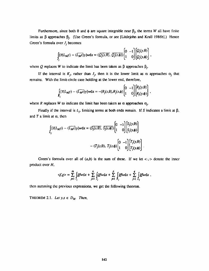
Furthermore, since both 0 and $ are square integrable near $j, the terms W all have finite
limits as $ approaches (3,. (Use Green's formula, or see [Littlejohn and Krall 1986b].) Hence
Green's formula over J, becomes
0 -1 Q3 (y,0)
J[z(Lnty') - (Luz)y]wdx = (Q(z,), Q(z,4)) ] y
where Q replaces W to indicate the limit has been taken as 0 approaches i.If the interval is Kj, rather than JI, then it is the lower limit as a approaches aj that
remains. With the limit-circle case holding at the lower end, therefore,
0 -1 R/(y,0)[z(Lmy) - (L z)ywdx = -(RJ(z,O),R,(z,$) 1 0 RJ(Y,$)J
where R replaces W to indicate the limit has been taken as a approaches a.
Finally if the interval is Lj, limiting terms at both ends remain. If S indicates a limit at $,
and T a limit at a, then
0 -1 SAY 1 0)j[(LMY) - (LMz)y]wdx = (S(z,0), S(z,$)) 1 0 S(y,)
0 -L T,(0)
-( T , , ) , T ( z ,$ ) 1 0 T ,(y ,$ ) '
Green's formula over all of (a,b) is the sum of these. If we let <-,-> denote the inner
product over H,
<f,g> =Xj-wx+ g-fwdx + P g-fwdx + I Jgfwdx,
then summing the previous expressions, we get the following theorem.
THEOREM 2.1. Let y,z e DM. Then,
142
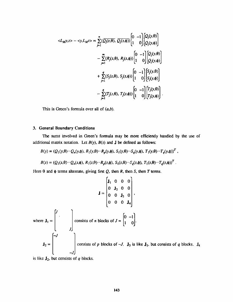
S0 -1 Q,)<LMy,z> - <y,LMz> = I(Q,(z,O), Q (z,4)) 1 0 ,o)
Fl
6 00 -1 Q,(,®)
- >(R(z,O), R(z,)) 1 0 Q,$)jF1
q 0 -1 S/,0)
+ X(S1 (z,O), S,(z) 1 0 ,$(Y)F1
q 0 -1 /y,O)- (T(z,O), T/(z,$)) 1 0 y jjy
This is Green's formula over all of (a,b).
3. General Boundary Conditions
The sums involved in Green's formula may be more efficiently handled by the use of
additional matrix notation. Let B(y), B(z) and J be defined as follows:
B(y) = (Q1(y,O)---Q,(y,4), R1(y,0)---R,(y,$), S1(y,O)---Sq(y,$), T1(y,O)---Tq(y,4 ))T ,
B(z) = (Q1 (z,O)-- Q(z,$), R 1(z,0)---R,(z,$), S1(z,O) --Sq(z,4), T(z,O)-- T(z,$)) T .
Here 0 and 4 terms alternate, giving first Q, then R, then S, then T terms.
Ji 0 0 0
0 J2 0 0
~=0 0 J3 0
0 0 0 J4
0 -1
where J1 = consists of n blocks ofJ= 1 0 -
-J
J2 = consists of p blocks of -J. J3 is like J1 , but consists of q blocks. J4
-Jlis like J2, but consists of q blocks.
143
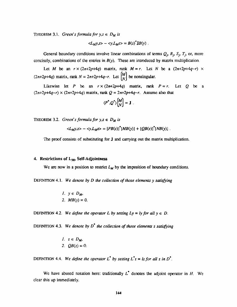
THEOREM 3.1. Green's formula for y,z e DM is
<LMy,z> - ZYLMz> = B(z)*JB(y) .
General boundary conditions involve linear combinations of terms Q1, R, S, Tj, or, more
concisely, combinations of the entries in B(y). These are introduced by matrix multiplication.
Let M be an r x (2n+2p+4q) matrix, rank M = r. Let N be a (2n+2p+4q-r) x
(2n+2p+4q) matrix, rank N = 2n+2p+4q-r. Let []be nonsingular.
Likewise let P be an r x (2n+2p+4q) matrix, rank P = r. Let Q be a
(2n+2p+4q-r) x (2n+2p+4q) matrix, rank Q = 2n+2p+4q-r. Assume also that
(P*,Q*) ] =J.
THEOREM 3.2. Green's formula for y,z e DM is
<LMy,z> - <yzLMZ> = [PB(z)]*[MB(y)] + [QB(z)]*[NB(y)].
The proof consists of substituting for J and carrying out the matrix multiplication.
4. Restrictions of LM, Self-Adjointness
We are now in a position to restrict LM by the imposition of boundary conditions.
DEFINITION 4.1. We denote by D the collection of those elements y satisfying
1. y e DM,
2. MB(y)=0.
DEFINITION 4.2. We define the operator L by setting Ly = ly for all y e D.
DEFiNITION 4.3. We denote by D* the collection of those elements z satisfying
1. z e DM,
2. QB(z)=0.
DEFINITION 4.4. We define the operator L' by setting L*z = lz for all z in D*.
We have abused notation here: traditionally L* denotes the adjoint operator in H. We
clear this up immediately.
144
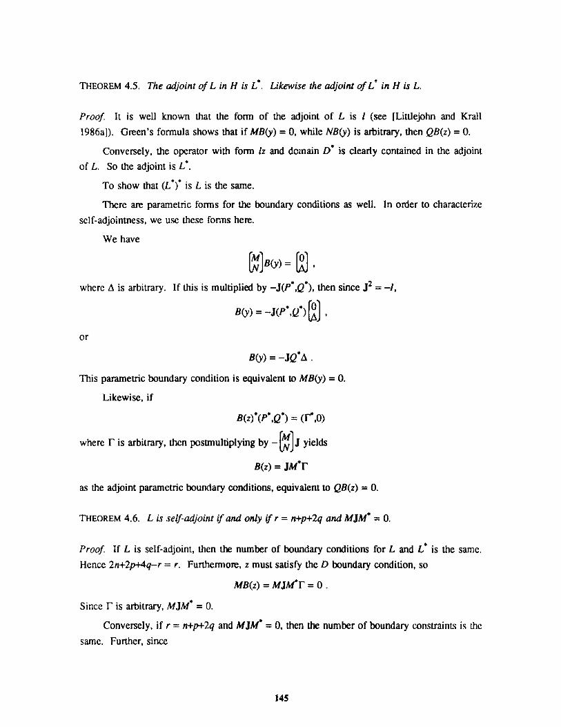
THEOREM 4.5. The adjoint of L in H is L*. Likewise the adjoint of L in H is L.
Proof. It is well known that the form of the adjoint of L is 1 (see [Littlejohn and Krall
1986a]). Green's formula shows that if MB(y) = 0, while NB(y) is arbitrary, then QB(z) = 0.
Conversely, the operator with form lz and domain D* is clearly contained in the adjoint
of L. So the adjoint is L*.
To show that (L )* is L is the same.
There are parametric forms for the boundary conditions as well. In order to characterize
self-adjointness, we use these forms here.
We have
B(y) =,
where A is arbitrary. If this is multiplied by -J(P*,Q*), then since J2 =_,
B(y) = -J(P*,Q*) ,
or
B(y) = -JQ*A .
This parametric boundary condition is equivalent to MB(y) = 0.
Likewise, if
B(z)*(P*,Q*) = (l,0)
where F is arbitrary, then postmultiplying by - J yields
B(z) = JM*
as the adjoint parametric boundary conditions, equivalent to QB(z) = 0.
THEOREM 4.6. L is self-adjoint if and only if r = n+p+2q and MJM* = 0.
Proof. If L is self-adjoint, then the number of boundary conditions for L and L is the same.
Hence 2n+2p+4q-r = r. Furthermore, z must satisfy the D boundary condition, so
MB(z) = MJM*f = 0 .
Since F is arbitrary, MJM* = 0.
Conversely, if r = n+p+2q and MJM* = 0, then the number of boundary constraints is the
same. Further, since
145
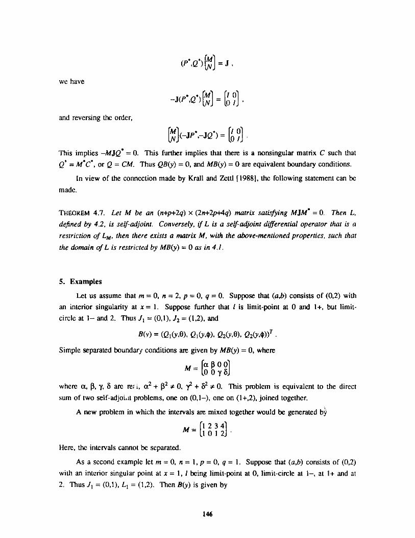
(P' Q*)N = J ,
we have
-NJ(P=,Q) ,11[
and reversing the order,
(-JP=,-JQ*) [I .This implies -MJQ* = 0. This further implies that there is a nonsingular matrix C such that
Q*= M*C% or Q = CM. Thus QB(y) = 0, and MB(y) = 0 are equivalent boundary conditions.
In view of the connection made by Krall and Zettl [1988], the following statement can be
made.
THEOREM 4.7. Let M be an (n+p+2q) x (2n+2p+4q) matrix satisfying MJM = 0. Then L,
defined by 4.2, is self-adjoint. Conversely, if L is a self-adjoint differential operator that is a
restriction of LM, then there exists a matrix M, with the above-mentioned properties, such that
the domain of L is restricted by MB(y) = 0 as in 4.1.
5. Examples
Let us assume that m = 0, n = 2, p = 0, q = 0. Suppose that (a,b) consists of (0,2) with
an interior singularity at x = 1. Suppose further that 1 is limit-point at 0 and 1+, but limit-
circle at 1- and 2. Thus J1 = (0,1), J2 = (1,2), and
B(v) = (Q1(y,0), Q(y,), Q2(y,O), Q2(y,))T
Simple separated boundary conditions are given by MB(y) = 0, where
M =
where a, $, y, S are re; 1, a2 + $2 # 0, 2 + S2 0. This problem is equivalent to the direct
sum of two self-adjoiat problems, one on (0,1-), one on (1+,2), joined together.
A new problem in which the intervals are mixed together would be generated by
r1234M= 1012J
Here, the intervals cannot be separated.
As a second example let m = 0, n = 1, p = 0, q = 1. Suppose that (a,b) consists of (0,2)
with an interior singular point at x = 1, 1 being limit-point at 0, limit-circle at 1-, at 1+ and at
2. Thus J1 = (0,1), L1 = (1,2). Then B(y) is given by
146
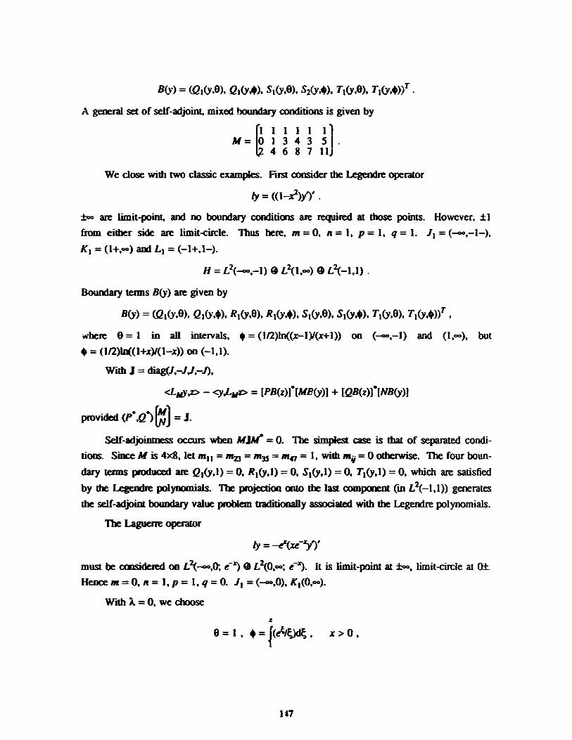
B(y) = (Q1(y,e), Q1 (y,), S(yO), S2(y,4), TI(y,O), T 1(y 4 ))T.
A general set of self-adjoint, mixed boundary conditions is given by
11 1 1 1 1
M= 01 3 4 3 5.4 6 8 7 11)
We close with two classic examples. First consider the Legendre operator
ly = ((1-x2 )y')'.
iyo are limit-point, and no boundary conditions are required at those points. However, 1
from either side are limit-circle. Thus here, m = 0, n = 1, p = 1, q = 1. J1 =(-,-1-),
K 1 = (1+,oo) and Lt = (-1+,1-).
H = L2(-co,-1) 0 L2(1,ca) 0 L2(-,)
Boundary terms B(y) are given by
B(y) = (Q1(y,0), Q,(y,$), R1 (y,0), R1(y,$), S1(y,0), S1(y,*), T1 (y,0), T(y,$))T,
where 0 = 1 in all intervals, $ = (1I2)ln((x-1)/(x+l)) on (-oo,-1) and (1,oa), but
* = (lI2)1t((1+x(1-x)) on (-1,1).
With J = diag(J,-J,-J),
<LMy,z> - <y,L z = [PB(z)fI[MB(y)J + [QB(z)f [NB(y)
provided (P',Q*) ]= J.
Self-adjointness occurs when MJM = 0. The simplest case is that of separated condi-
tions. Since M is 4x8, let m1 1 = m23 = m35= m47= 1, with m = 0 otherwise. The four boun-
dary terms produced are Q1(y,l) =0, R1(y,l) =0, S1(y,l) = 0, T1 (y,1) =0, which are satisfied
by the Legendre polynomials. The projection onto the last component (in L2(-1,1)) generates
the self-adjoint boundary value problem traditionally associated with the Legendre polynomials.
The Laguerre operator
ly = -e(xe~y)'
must be considered on L2 (-<o,0; e~&) 0 L2(0,oo; e~X). It is limit-point at to, limit-circle at 0 .Hence m = 0, n = 1, p = 1, q = 0. J1 = (-o,0), KI(0,oo).
With ?=0, we choose
8 = 1 , $= (el/()dt, x > 0,
147
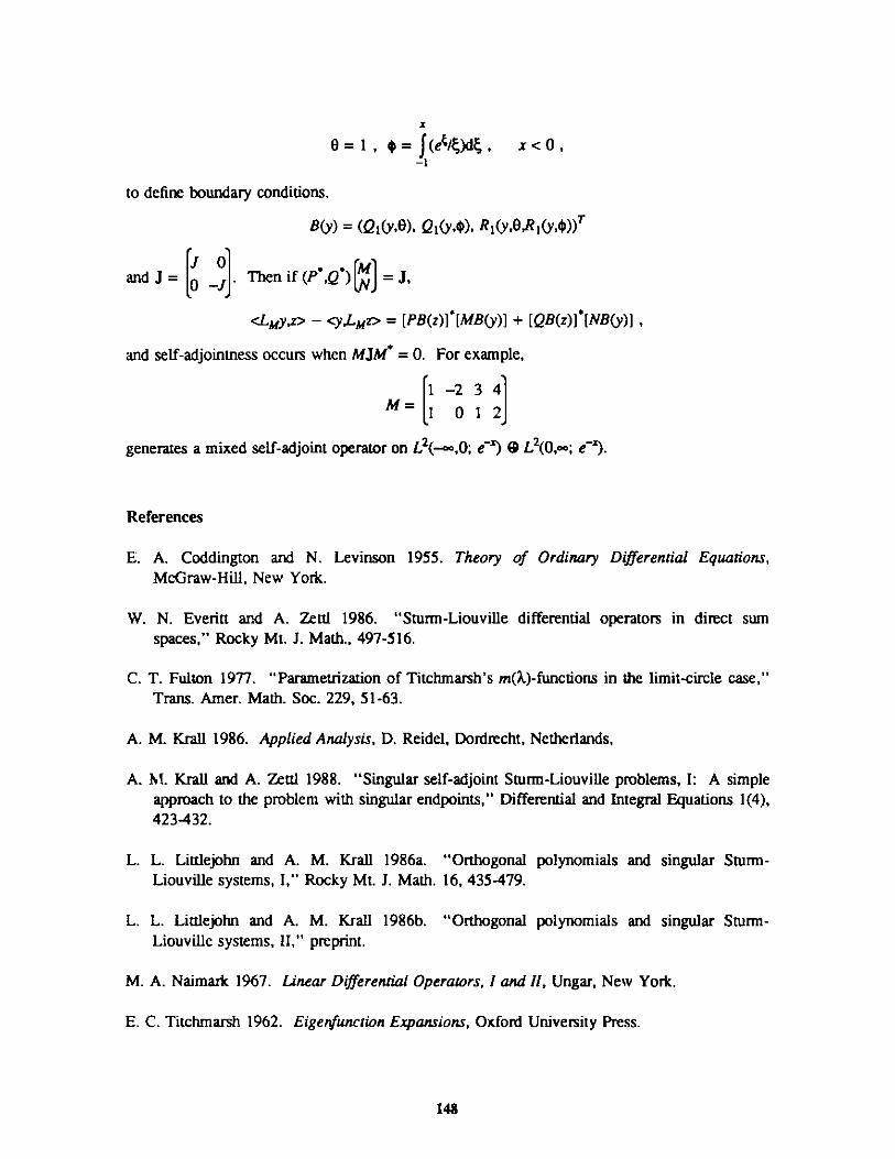
0= 1 , $"= (et)d , x < 0,
-1
to define boundary conditions.
B(y) = (Q1(y,0), Q(y,$), R1 (y,0,R 1(y,))T
and J = 0 -J . enif (P*,{jJJ[J 0J
<LMy,z> - <yLMr> = [PB(z)]f[MB(y)] + [QB(z)]f[NB(y)] ,
and self-adjointness occurs when MJM* = 0. For example,
1 -2 3 4M= 1 0 1 2
generates a mixed self-adjoint operator on L2 (-<=,0; e~ ) @ L2 (0,oo; e").
References
E. A. Coddington and N. Levinson 1955. Theory of Ordinary Diferential Equations,McGraw-Hill, New York.
W. N. Everitt and A. Zettl 1986. "Sturn-Liouville differential operators in direct sumspaces," Rocky Mt. J. Math., 497-516.
C. T. Fulton 1977. "Parametrization of Titchmarsh's m(X)-functions in the limit-circle case,"Trans. Amer. Math. Soc. 229, 51-63.
A. M. Krall 1986. Applied Analysis, D. Reidel, Dordrecht, Netherlands,
A. M. Krall and A. Zettl 1988. "Singular self-adjoint Sturm-Liouville problems, I: A simpleapproach to the problem with singular endpoints," Differential and Integral Equations 1(4),423-432.
L. L. Littlejohn and A. M. Krall 1986a. "Orthogonal polynomials and singular Sturm-Liouville systems, I," Rocky Mt. J. Math. 16, 435-479.
L. L. Littlejohn and A. M. Krall 1986b. "Orthogonal polynomials and singular Sturm-Liouville systems, II," preprint.
M. A. Naimark 1967. Linear Differential Operators, I and II, Ungar, New York.
E. C. Titchmarsh 1962. Eigenfunction Expansions, Oxford University Press.
148
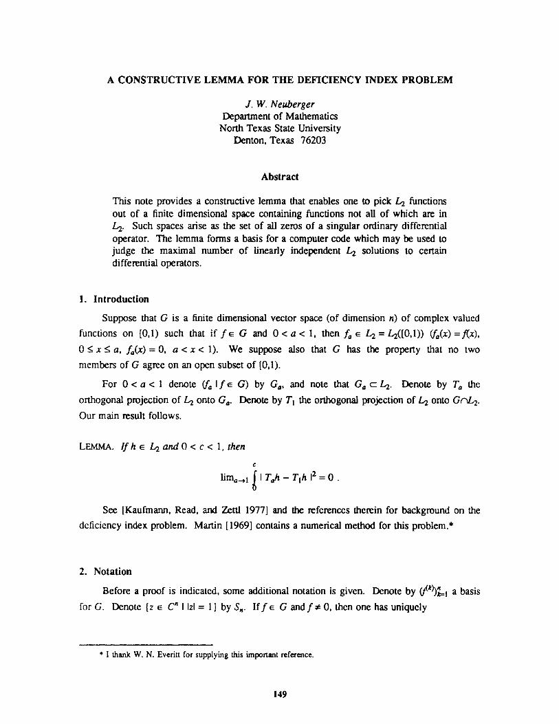
A CONSTRUCTIVE LEMMA FOR THE DEFICIENCY INDEX PROBLEM
J. W. NeubergerDepartment of Mathematics
North Texas State UniversityDenton, Texas 76203
Abstract
This note provides a constructive lemma that enables one to pick L2 functionsout of a finite dimensional space containing functions not all of which are inL2 . Such spaces arise as the set of all zeros of a singular ordinary differentialoperator. The lemma forms a basis for a computer code which may be used tojudge the maximal number of linearly independent L2 solutions to certaindifferential operators.
1. Introduction
Suppose that G is a finite dimensional vector space (of dimension n) of complex valued
functions on [0,1) such that if fer G and 0 < a < 1, then fa E L2 = L2([0,1)) (fa(x) = f(x),
0 x 5 a, fa(x) = 0, a < x < 1). We suppose also that G has the property that no two
members of G agree on an open subset of [0,1).
For 0 < a < 1 denote (falf E G) by G, and note that Ga cL2 . Denote by Ta the
orthogonal projection of L2 onto Ga. Denote by TI the orthogonal projection of L2 onto GrL2 -Our main result follows.
LEMMA. If h E L2 and 0 < c < i, then
c
lima._,i ITah - T ih12 = 0 .
See [Kaufmann, Read, and Zettl 1977] and the references therein for background on the
deficiency index problem. Martin [1969] contains a numerical method for this problem.*
2. Notation
Before a proof is indicated, some additional notation is given. Denote by (/k))Li a basis
for G. Denote (z e C" I Iz = 1) by S,. If f E G and f * 0, then one has uniquely
* I thank W. N. Everitt for supplying this important reference.
149
R
f=pL_ where p>0 and f= zkIk, z=(z 1 ,...,z.)e S.
Note that if0< c< 1, then there isM suchh that iff#0,fe G, thenJ0 IL 12 Mc.
3. Indication of Proof of Lemma
Suppose that h E L2 and 0 < a < 1. Write Tah = r(a) + s(a), where r(a) is the nearest ele-
ment (using L2 norm) in Ha = ff. If E GrnL2}to h. Consequently, s(a) E Gar H. In fact, s(a)
is the nearest element of Ga JI to h.
Suppose now that 0 < c < 1. It is to be shown that
C
lima_,51Is ()12 = 0 .
For 0 < a < 1 and s(a) # 0,
s(a) =11s(a)1- 2 < h , s(a) > s()
and consequently,
Is ()2 = Is(a)II- 2 I < h, s(a) > 12 Is()1 2 / ()2
S11h11 2 I(a)I2 / ( )2
It will be established that
lima--1I ()2 = , (*)
the limit being taken over values where s() 0 (if there is not an increasing sequence of such
values converging to 1, then surely lima-.. JII s()I 2 = 0).
Suppose that (*) does not hold in the indicated sense. Denote by M a positive number
and by (ak}1 an increasing sequence in [0,1) converging to I so that
a
kI&(a12 < M, k = 1,2,... .
Denote by d a member of [0,1), and denote by K a positive integer such that ak > d if
k > K. Then {Zk)} .. is a bounded subset (in L2 sense) of the finitie dimensional subspace
Gd of L2. Hence for some subsequence (bk)*1 of {ak)I, (k )}' converges in L2 to a
150
member g of Gd for some member g E G. Clearly, |gldIl|< M. If d < q < 1, then an examina-
tion of {() }=i reveals that this sequence converges in L2 to gq (consider members of these
sequences expanded in terms of the specified basis with coefficients in S). Hence it must be
that g E L2 since Igg|| M for all d < q < 1. Moreover, g * 0 since gd may be expanded in
terms of the basis (f/A)11 with coefficients in S,.
It is shown next that { sb")} i converges weakly to g. Suppose u e L2. Then
<u,s - g>I < <u - ud( k) - g>I+ <ud,S(b - g>I
5 2M lul2 + I <u, k - gd> -+ 0 as d -+ 1
d
Hence, if v e GrVL 2 , <v,g> = limk,,..<v,h *> = 0 since by construction (** is orthogonal to all
of GrVL2 . But this gives a contradiction, since it was shown that g E Gr 2. Therefore, the
above assumption is false, and consequently
a
lima_,1 1(a) 2=
From the inequality J1s(a)<2 | h112 f- I (a)I2 /J ()2, it then follows that lima_ 1J Is(a)1 2 = 0
since f,(a)12 must remain bounded as a -* 1.
Recalling that if 0 < a < 1, then r(a) is the nearest element to h which is in (falf E GrL}
and that T1h is the nearest element to h which is in GrVL2 , one sees that
C
lim ITlh - r(a)12 = 0.a-+1
Hence
c c
IT1h - Tahl2 = ITth - r(") - s(a)I2
c c
IT~h - r(a)12 + [ Is(a)2
-+0 as a -+ 1 .
This completes an indication of proof.
151
4. Applications
In applications, G may be the set of all zeros of a differential operator of order n which
has a sole singularity at 1. A basis for G is obtained by solving the resulting differential equa-
tion for n linearly independent sets of initial conditions at 0. An element h of L2 is chosen.
The resulting Tih is constructively identified as an L2 limit over each subinterval [0,c],
0 < c < 1. After Tih is found, then the process is repeated with a new h which is orthogonal
to the previous Tih found. At any step several choices for h probably should be considered
since it is possible that a given h may be orthogonal to all L, members of G which have not
yet been found.
5. Computer Code
In a personal communication, W. N. Everitt suggested that a computer code dealing with
the deficiency index problem might be helpful. Toward this end, discussions at Argonne
National Laboratory in March 1987 were invaluable. The resultant code, called BMGHM
(BirMinGHaM), was written at Birmingham University during June 1987, and the idea behind
this code was explained at the University of Cardiff shortly thereafter. In its present form the
code applies only to a second order operator, but there seem to be no obstacles to a code being
written that follows the above lemma in a rather general setting.
References
R. M. Kaufmann, T. T. Read, and A. Zettl 1977. "The deficiency index problem for powersof ordinary differential expressions," Lecture Notes in Mathematics, Vol. 621, Springer-Verlag, New York.
E. M. Martin 1969. "On the numerical and theoretical determination of deficiency indices ofordinary differential equations," M.Sc. thesis, Dundee University.
152
SPECTRAL PROPERTIES OF NOT NECESSARILY SELF-ADJOINTLINEAR DIFFERENTIAL OPERATORS*
Bernd SchultzeFachbereich Mathematik
University of EssenEssen, West Germany
Abstract
For a large class of not necessarily symmetric linear differential expressions (hav-ing powers of the independent variable as dominating coefficients) the nullitiesand the essential spectrum are exactly determined. This generalizes the results inthe constant coefficient and in the Euler case due to Balslev and Gamelin (PacificJ. Math. 14, 1964, 755-776).
We consider not necessarily self-adjoint singular differential operators generated by ordi-
nary differential expressions of the form
P
My = I p(t)y( ) on 1 = [1,oo) (*)i=0
with n = ord (M) e N, p; E C (I, C). With M+ we denote the adjoint expression
M~y = ((-1)(p;(t)y)(i=0
and with T0 (M) and T 1 (M) the minimal and maximal operator, respectively, generated by M in
L2(1). The basic spectral and extension theory (even in LP-spaces) was given by Rota [1958]. In
this theory the essential spectrum of M,
ae(M):= ( e C I range T0 (M-) is not closed),
plays a crucial role. If we assume that this set is not the entire plane, the following integers
nul(M-X):= dim ker T1 (M-4)
tum out to be constant (as functions of A) on each connected component of C \ ae(M). These
numbers are important because they indicate how many linearly independent boundary conditions
one has to impose for a restriction of T 1 (M) (resp. an extension of T0 (M)) in order to obtain a
so-called maximal extension, i.e., an extension with minimal spectrum in this component. These
*Part of this work was done while the author was a visiting professor at Northern Illinois University, DeKalb,Illinois, during 1985-1986. This stay was also supported by a Fullbright travel award.
153
maximal extensions correspond to the self-adjoint extensions in the symmetric case, and Rota has
shown that in the component where the maximal extension is taken, the spectrum consists of an
(at most) countable number of eigenvalues having only points of a,(M) as possible accumulation
points.
To apply this theory in concrete cases, we must determine these spectral data ae(M) and
nul(M-X). In the non-selfadjoint case, the only large classes of expressions where these spectral
invariants have been completely evaluated are the constant coefficient expressions and the Euler
expressions, together with their relatively compact perturbations. This evaluation was achieved
by Balslev and Gamelin [1964]; see also Goldberg [1966]. Even in the symmetric case, the
classification of these spectral invariants in terms of the coefficients of the expression is far from
complete. The results presented here consist of an exact evaluation of the essential spectrum and
the nullities of a large class of expressions having real powers of the independent variable as
dominating coefficients. This paper generalizes the results of Balslev and Gamelin to a much
larger class of expressions in the L 2 -case. Comparison with certain symmetric expressions will
also show that this type of result cannot hold for all expressions of the class mentioned above.
We give here only the principal ideas of the theory, omitting the proofs which are rather technical
in detail.
1. Special Expressions
We first consider expressions of the form
MOY:= I act y Y/(1.1)
a=O
with r e N,Po,...,Pr E No,0 0 = po < p1 <... < pr = n and ae R(a = 0,...,r) such that
o = 0, ai P1 (1.2)
and
1- > fora=,...,r-if r > 1 . (1.3)Pa&Pa-I P0+i1 P
Let us denote by al < ... < a,_1 those indices a (a = 1,...,r -1) for which the strong inequality
holds in (1.3). Then together with ao:= 0, a,:= r we have
= for a1_1 < a5 a1 (j = 1,...,s) ifs>_1 (1.4)Pa,--Pa, Pa-Pa-1
and
>_' for j = 1,...,s-1 if s > 2 . (1.5)Pa-Pa 1 - Pa,., -Pa,
Now we are in the position to formulate the assumption on the constants a0 e C \ [0):
154
afaE R \(0) for a =a , - - - ,,r and for each k = p0 ,,...,n we have
ck:= I (-1)P+k a wa x 0 (p ,k, , i1,..,s-) (1.6)
p.+px=2ka,5ic, X62a,
The ca(a = 0, ... , al-1) may be arbitrary complex constants.
A condition sufficient for (1.6) to hold is the following simpler condition:
sgn((-1)Paa%) = const for all a al such that pa is evenp +1 (1.7)
sgn((-1) 2 a) = const for all a ? al such that pa is odd .
In the following, we will call an expression Mo of the form (1.1) satisfying (1.2), (1.3), and (1.6)
a special expression (using 0 0,s...,a as subscripts for the "kink-indices"). Our first goal is to
derive a lower estimate of IMo f 12, where M0 is an arbitrary special expression and
f e Co0(rj,oo), i.e., f belonging to the set of all indefinitely differentiable functions having com-
pact support in the interval (1, ) for some 11 1. Since 11Mo f II 2 = (MMo f,f), where (, )
denotes the usual inner product in L2 (I), we investigate the Dirichlet-integral of the symmetric
expressions MoMo. Its structure is given by Frentzen [1987] generalizing a lemma of Read
[1982] to the general complex coefficient case:
LEMMA 1. Let M be given as in (*) with pi e C"(I,C) (i=O,...,n). Then MM is of the form
n n -1
M+My = (-1)k(gy(k))(k) + i ( 1)k((~y(k))(k+l) +~(k*k))()}k =O k =O
with
qk = (-1)i+kAijRe(,ipj) + (-1)i+k cij,kReipj)(i+j-2k)i+j =2k 2j i+j>2k22j
qk = (-1)c'ij,k Im ipj)(i+j-1-2k)i+j-1 2k 2j
for 0 <-k n (resp. n-I) , whereAij:= .or and cij,k, c j,k are certain constants.
Applying this to a special expression M0 , we get for the coefficients qk (k = 0,..., n) of
n n-1
MjM0 y = (-1)k(qky(k))(k) + iE( -)k('ky(k))(k+) + (~j9(k+1))(k)) (1.8)k=0 k=0
the following representation.
PROPOSITION I. If Mo is a special expression and qk (k = 0, ... ,n) the coefficients of the real part
of MojMo given by (1.8), then for pa, 5 k pa, (i = 1,...,s-I) there exists ck -0 such that
155
qk(t) = (Ck + ((1))t.9)
with cp, = a2 (i = 1,...,s) and y;, := 2 {k-p0)oG + (pa. - k)%,), and forPa,,, - pa
k = 0,...,pa, -1 we have
2k-
qk(t)=0 t J (1.10)
If, furthermore, (1.6) holds also for a = 0,...,a-1, 0 k pl, then (1.9) is also valid for this
range of the k's.
This information-together with a similar representation of the q, which follows from
Lemma 1, and inequalities derived by Schultze [1984] (see also Merger and Schultze [1986: Sec-
tion 51)-gives the crucial estimation.
PROPOSITION 2. If M0 is a special expression, then there are constants bk > 0 (k = 0,...,n),
K 0, and e I such that for allf E Co (T),oo) we have
s-i Po+IIM0 fll i2 E fbkt 4 Iftk)I2+(bo -K) I f I I2 . (1.11)
i=Ok=p,,, I
If, furthermore, (1.6) holds also for a = 0,...,a1, 0 5 k ! p,, then we can choose K = 0.
2. Perturbations of Special Expressions
Proposition 2 enables us now to identify expressions
My = rky k)(2.1)k =0
with rk e Ck(I,C) (k = 0,...,n) and
rk(t) - o(tA 4) (2.2)
for k = 0,...,n and i = 0,...,s-1 such that pa, k 5 p,,, as relatively bounded (resp. relativelycompact) perturbation of the special expression MO (defining the y;,k as in Proposition 1 for
i = 0,...,s -1,k = 0,...,n).
For the invariance of the nullities, we can admit a somewhat less general class of perturba-
tions consisting of expressions (2.1) satisfying
r )(t) = o(t/'2i" ) (2.3)
for k = 0,...n; j = 0,...,k, and i = 0,...,s-1 such that pa, <k-j pg.. Condition (2.3) is
fulfilled, e.g., by expressions satisfying (2.2) with ra(t) = o(t 1~&j) (j = 0,...,k), that is, having a
behavior for the derivatives of the coefficients similar to powers of t. Simple estimations give the
156
(1.9)
following implication of Proposition 2.
LEMMA 2. Let MO be a special expression and M a corresponding expression, i.e, of the form
(2.1) satisfying (2.2). Then
there exists 1E 1, 0 < a < 1, a >_0 such that for all(fe Co'(,oo) we have 11Mf11 2 <-a IIMofI 2 +( $11f 112 .J (2.4)
With standard conclusions we obtain the following.
REMARK 1. If M and M0 satisfy (2.4), then
domain (T0 (M0 + M)) = domain (T0 (M0 )) .
The basic perturbation theorem that we apply here is due to Kauffman [1977]; we cite it in a form
convenient for our purpose.
PROPOSITION 3. Let M be given as in (*) with p(t) #0 on I and range T0 (M) closed. Let N be
another expression of form (*) with order N < order M satisfying the following condition. There
is a g e C(I). g > 0 and limg(t) = 0 such that gNf E L2 (I) for all f E domain To(M). Then the
operator, defined as the restriction of N on domain T0 (M), is relatively compact with respect to
T0(M), and we have domain T0 (M+N) = domain T0 (M), nul (M + N+) = nul M+ and
range TO(M+N) is also closed.
Using Proposition 2 to satisfy the condition in the assumption of this proposition, we obtain
the following.
PROPOSITION 4. Let M0 be as special expression and M a corresponding perturbation, i.e., an
expression of the form (2.1) satisfying (2.2). Then Ge(Mo+M) = a,(Mo). If M satisfies even
(2.3), then also nul (MO+M-X) = nul (M0-A) for every X e C \ ae(Mo).
In the proof of this proposition, we have to surmount several obstacles. So the order-
condition of Proposition 3 can be established considering the expression (1 + t r (t)) (M0-4)
instead of M0 - X. Also for the invariance of the nullities, we remark that Moj itself is a perturba-
tion of a special expression A170, and (2.3) asserts that (2.2) holds for M+. So applying Proposi-
tion 3 to A1'o - , we obtain this assertion.
3. Results
Now we focus our attention on special expressions to obtain their essential spectrum and
nullities, since the preceding section enables us to translate these results to much more general
expressions. We determine these spectral data by successive factorization modulo relatively com-
pact perturbation in the following sense. If M0 is given as in (1.1) satisfying (1.2), (1.3), and
157
(1.6), then we define
0-
N y: = _ a O "yE "' for i = 1,...,sa=O
and
N;y: = + ta ~' y'('P') for i = 1,...,s-l (ifs > 1) .Yao,+1 a(,;
N and N;, 1 + 1 are special expressions, and N, 1 + I satisfies even (1.6) for all indices. Proposi-
tion 2 implies therefore that range (T0 (N, l + 1)) is closed; and since I contains one of its ena-
points, we have that T, (Ni,,I + 1) is surjective. If i < s, we have with
111 := N; N;,1 - (N; +1 - N;) - XN;,i, A XE C
(N; - ))(N;, l + 1) = N;1 + 1; i- A,
and 117 satisfies (2.2) and even (2.3), since the coefficients are powers of t, corresponding to Ni1 .Proposition 4 therefore yields
XE C \ ae(Ni+1) range (To((N; - X)(N;, 1 + 1))) closed T 1 ((N; - X)(N, + 1)) surjective .
Now, N, 1 has the following property: Nt+1 N;, 1 is limit-point [Schultze 1984: 7.1, 7.2c], and
therefore N;, 1 is limit-point in the generalized sense (see [Frentzen 1987]).
Proposition 4 also indicates that N;, 1 +1; - X is limit-point in the generalized sense. So let
f e domain T (N;+1 + 1?; - a) = domain T 1 ((N; - A)(N, + 1)). Then, by [Kauffman, Read, and
Zettl 1977: Corollary 4.7] there exist g E Co (l) with f - g E domain
To(N,+1 + v7; - X) = domain TO(N;, 1). Proposition 2 then shows that N, i f E E2(1). These con-
siderations imply that T (N; - A)T 1(N;, + 1) = T ((N; - A)(N, + 1)), since the other inclusion
is trivial. So we have finally a,(Ni+1) = ae(Ni) and for ? E C \ a,3(N;)
nul (N;+1 - A) = nul (N; - X) + nul (N;,1 + 1) .
Defining
a,
Moey:= a0 ty " (3.1)C=O
the essential part of M0, and if s > 1,
158
M;y:= ct y (i = 1,...,s-), (3.2)a=a
we have shown the following.
PROPOSITION 5. Let Mo be a special expression as in (1.1). Then ae(Mo) = ae(Mo, ), and for
A. CE\ae(Mo) wehave
s-1nul (Mo -) = nul (Mo,, -X)+ nul (M;).
i=1
There remains the problem of finding the essential spectrum of Mo., and the nullities of
Moe - X, M; (i = 1,...,s-1), i.e., of special expressions without kinks: Noy =
a at y , -P =a (a = 2,...,a1). Considering first the case a1 < pi (the expressions M;(T=O Pa Pi
(i = 1,...,s-1) are in this case), we define the following polynomial associated with No:
a P ,
p (z) = E a azP" = aa, TI1 (z -X;)
a=0 = Pa 1 l
together with its decomposition into linear factors. Define t:=--- < 1 and Ly: = t y'. Thena1
similar arguments to those proving Proposition 5 show that p(L) is a relatively compact perturba-
tion with respect to No. So Rota's spectral mapping theorem yields ae(p(L)) = p(a,(L)), but
since a,(L) = iR, we obtain
a
a,(No)= ( aazP IRe z = 0a=0
a
On the other hand, p(L) = a a, H (L - ?) gives alsoi=o
a,
T 1(p(L))=a., H T1(L-Xi),
and so we have
a,
nul(No)=# z I aazP=0, Rez <0.a=o
This together with Propositions 4 and 5 gives our first main result.
THEOREM 1. Let Mo be a special expression given by (1.1) satisfying (1.2) with a1 <p l, (1.3)
and (1.6). Let M be an expression of the form (2.1) satisfying (2.2). Then
159
a,(Mo + M) = a,(Mo) = I a azP" I Re z = 0.
a=o
If M satisfies (2.3), then for every ? E C \ a,(Mo)
a
nul(Mo+M-)=nul(Mo-X)=# zI azP = Rez <0a=o
S -1 G++ '# (zi aoz ~a' = 0, Rez <0
i=1 a=a
For ai = pi, Mo,e is an Euler expression whose essential spectrum and nullities have been deter-
mined by Balslev and Gamelin [1964] using the linear isometry induced by the classical transfor-
mation to the constant coefficient case. Making use of their result (see also Goldberg [1966]), we
obtain the following theorem.
THEOREM 2. Let Mo be a special expression given by (1.1) satisfying (1.2) with a! = p , (1.3)
and (1.6). Let M be an expression of the form (2.1) satisfying (2.2). Then
a, a-1ae(Mo+M)=ae(Mo)= as H (z-'A-j) I Rez=0}.
a=0 j=0
If M satisfies (2.3), then for every X E C \ ae(MO)
a, a-1nul(Mo+M-A)=nul(Mo-.)=# zI Fa; H (z-'A-j)=A, Rez <0
a=0 j=
s -i r a;++ # zI Y azP" " =0, Rez <0.
i=1 a=a
REMARK. The assumption ao = po = 0 is only a technical one, and all the assertions of the
preceding theorems remain valid without this condition.
This kind of result is no longer valid for expressions that do not satisfy Condition (1.6), as
the following simple example shows. Ny: = y (4) + (xy 3' - y(4) + xy''+y ' is a symmetric expres-
sion onI and therefore 2 < nul (N-i). But since in our theory Moy:= y(4) +xy'' and My:= y' a
corresponding, relatively compact perturbation, Theorem 1 would imply nul (N-i) = #(Z2Re z < 0} + #(z I z2 = -1, Re z < 0) = 1 +0 = 1, contradicting 2:5nul (N-i).
REMARK. The number of zeros of a polynomial Q of order n with negative real part determining
the nullities in the above theorems c.n be computed by means of the argument principle:
160
#(z IQ(z)= 0, Re z <0)=-2 +var (arg Q(is)I- < s <oC} .2
This is very useful for the computation of the nullities.
4. The Case a1 > p1
If we consider expressions of the form (1.1) having growth points (p;,g) above the bisec-
tor, things become rather different. First a generalization of Hardy's inequality shows that terms
"lying" below the line with slope 1 that passes through (p 1,a) can and should be considered to
be relatively compact perturbations. So in the case ai > pr we define
0:=max(a;-p; Ii=0,...,r)>0 (4.1)
T:= i( ag- p; = , a; *0)
and
S:= max(i I i E =T). (4.2)
REMARK. We have
s=0 or c=(1 ,. (4.3)
Expressions M0 as in (1.1) satisfying (1.3), (1.6), and (4.1) are no longer special expressions in
the sense of Section 1, but we can associate a special expression with them:
Mo,y:= t 1 Mo=y =t 'M oy". (4.4)
Mo s is a special expression having as an essential part an Euler expression if and only if T = a.
For the admissible perturbations of Mo,
My = ry(k) (4.5)k=o
with rk e Ck(IC) (k = 0,...,n), we claim
rk(t) = o(t'Y) if i="1-,...,s-I exists with p -k < pa01 (4.6)o(t ) for k=0,...,p4
or, resp., for j = 0,...,k,
= o(t:' ') if i=t- ,...,s-1 exists with pa S k-j S p,
o(t -) fork =,...,p . (4.7)
It is evident that M satisfies (4.6) (resp. (4.7)) with respect to MO if and only if tUM satisfies
161
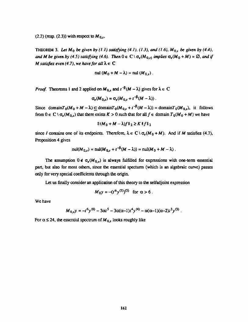
(2.2) (resp. (2.3)) with respect to Mo J.
THEOREM 3. Let Mo be given by (1.1) satisfying (4.1), (1.3), and (1.6), Mo,s be given by (4.4),
and M be given by (4.5) satisfying (4.6). Then 0 E C \ a,(Mo.s) implies a(J(Mo + M) = 0, and if
M satisfies even (4.7), we have for all A E C
nul (Mo + M - A)= nul (Mo.,).
Proof. Theorems 1 and 2 applied on Mo,s and t-(M - A) gives for A e C
ae(Mo,) = a,(Mo,s + t (M - A)).
Since domainT0(M0 + M - A) c domainTo(MO, + t 0(M - A)) = domainT0 (M0 ,1 ), it follows
from 0 E C \ a,(Mo,s) that there exists K > 0 such that for all f e domain T0(M 0 + M) we have
:!(MO +M -A)f2112 KI~f I 2
since I contains one of its endpoints. Therefore, A e C \ a,(Mo + M). And if M satisfies (4.7),
Proposition 4 gives
nul(Mo.,) = nul(Mo,, + t4 (M - A)) = nul(M0 + M - A) .
The assumption 0 4 a,(Mo.,) is always fulfilled for expressions with one-term essential
part, but also for most others, since the essential specturm (which is an algebraic curve) passes
only for very special coefficients through the origin.
Let us finally consider an application of this theory to the selfadjoint expression
Moy = -(tQy( 3)P) for a > 6.
We have
Mosy = -t 6y(6) - 3S - 3ac-1)t4 y(4) - a-1 -)3y(3)
For a :524, the essential spectrum of Mo,s looks roughly like
162
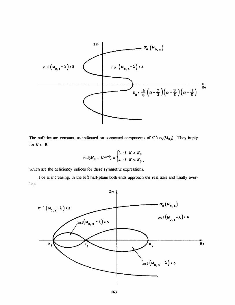
Im
nul(M0 , -X) =3
oe, (M)os
nul(M 0 -x) = 4
Re15 79 II R
K -8 2 2
The nullities are constant, as indicated on connected components of C \ a,(Mo,s). They imply
for K e R
3 i f K <Ko
nul(Mo- Kt6)={4 if K > Ka ,
which are the deficiency indices for these symmetric expressions.
For a increasing, in the left half-plane both ends approach the real axis and finally over-
lap:
Im
K2 K
cul(M =)
nul(M 098 X=
ReK0
nul (M, , - X) =3
163
v mdmqob, i --f. so
nul(M -~
nu l( M ,s- A=
a = 25 is the first integer where this happens. For this value of a we have K 1 = -1599360,
K2 = -1771200. Looking at the deficiency indices of Mo + Kt" we have
3 for K > -K 2j5 for -K1 < K < -K 2nul(Mo0+ Ktc) = 3 for -K0 < K < -K 1
4 for K<-K0
We see that for some positive K this expression is not limit-point. It was a long-time conjecture
that formally selfadjoint expressions with positive coefficients are always limit-point. In the
second order case this has already been proven by H. Weyl. Kauffman [1977] has shown for just
the expression we are considering in our example that K > 0 and a > 6 exist such that a necessary
condition for the limit-point case is not fulfilled, giving a counterexample to the conjecture.
Application of Theorem 3 gives even the deficiency index explicitly and the corresponding values
of the parameter a and K. This was also done by Paris and Wood [1981] using sophisticated
asymptotic methods.
References
E. Balslev and T. W. Gamelin 1964. "The essential spectrum of a class of ordinary differentialoperators," Pacific J. Math. 14, no. 3, 755-776.
H. Frentzen 1987. "Limit-point criteria for not necessarily symmetric quasi-differential expres-sions," preprint.
S. Goldberg 1966. Unbounded Linear Operators, New York: McGraw-Hill.
R. M. Kauffman 1977. "On the limit-n classification of ordinary differential operators with posi-tive coefficients," Proc. London Math. Soc. (3) 35, 496-526.
R. M. Kauffman, T. T. Read, and A. Zettl, 1977. "The deficiency index problem for powers ofordinary differential expressions," Lecture Notes in Mathematics, Vol. 621, Berlin,Springer-Verlag.
B. Mergler and B. Schultze 1986. "On the stability of the limit-point property of 'Kauffmanexpressions' under relatively bounded perturbations," Proc. Roy. Soc. Edinburgh 103A, 73-89.
R. B. Paris and A. D. Wood 1981. "On the L2 nature of solutions of n-th order symmetricdifferential equations and McLeod's conjecture," Proc. Roy. Soc. Edinburgh 90A, 209-236.
T. T. Read 1982. "Positivity and discrete spectra for differential operators," J. Diff. Equations43, 1-27.
164
0. C. Rota 1958. "Extension theory of differential operators," Comm. Pure Appl. Math. 11, 23-65.
B. Schultze 1984. "Ordinary differential expressions with positive supporting coefficients,"Habilitationsschrift.
165
ANALYSIS OF THE ASYMPTOTIC BEHAVIOR OF THELINEARIZED STAGNATION FLOW EQUATION OF THE
KURAMOTO-SIVASHINSKY TYPE
E. SocolovskyDepartment of Mathematics
University of PittsburghPittsburgh, PA 15260
G. K. LeafMathematics and Computer Science Division
Argonne National Laboratory9700 South Cass AvenueArgonne, IL 60439-4844
Abstract
The study of extinction and stability limits of premixed flames in stagnation pointflow lead to a nonlinear evolution equation describing the amplitude of the flamefront [Sivashinsky, Law, and Joulin 1982]. In this investigation we restrict ourattention to the one-dimensional linear eigenvalue equation. In particular weinvestigate the possible asymptotic behavior of solutions to this equation atinfinity. We present the leading behavior of the four independent solutions withtheir parametric dependence clearly displayed. Two asymptotic methods ofanalysis are presented. In the first section we use a generalization of the methodsof Laplace and steepest descent to obtain the leading behavior at infinity. In thesecond section we use the WKB method to obtain the leading behavior at infinity.
These results are needed in determining appropriate boundary conditions toapproximate the problem in a finite domain and devise computational schemes tostudy the behavior of the eigenvalues, in particular the conjecture on a Hopfbifurcation [Kaper and Schultze 1987].
* Assistant Scentist, Mathematics and Computer Science Division, Argonne National Laboratory, June 1 -
September 2, 1987.
/ ('6_1 lo
1. Asymptotic Approximation Using Laplace Contour Integrals
1.1. Introduction
In this section we formally find solutions to
$4)()+ -142)(x)+ -ax (1)(x)+ (a+A) $x) = 0, 0< x< oo , V> 0, (1.1)V v v
in the form of Laplace contour integrals, and then asymptotically approximate these using a
steepest descent or a Laplace technique.
There is an extensive literature on these "classical" methods and their application. As
references for the standard techniques we may mention [Wasow 1965; Carrier, Krook, and
Pearson 1966; Copson 1965; Murray 1984; Bruijn 1981] among others. From the application
papers we selected [Rabenstein 1958] which deals with a fourth order equation related to the
Orr-Sommerfeld equation of hydrodynamic stability.
A generalization of the method of steepest descent, in which the exponential kernel is
replaced by any transcendental or entire function, is given in [Bleistein 1972]. Here we use
extended applications of the methods since our exponential kernel is of the form exp[ah(w,1)]
instead of the usual exp[Ah(w)], where X is the "large" parameter.
An outline of the rest of this section is as follows. In Subsection 1.2 we find Laplace
contour solutions of (1.1); i.e., we determine the integrand and admissible contours. In Sub-
sections 1.3 we 1.5, we obtain three solutions and their asymptotic approximation using the
steepest descent method, which is outlined in Subsection 1.3. In Subsection 1.5 we briefly
describe the behavior of the steepest descent contours, and in Subsection 1.6 we then discuss a
fourth contour and asymptotically approximate the solution by a variation of the Laplace tech-
nique. Finally, in Subsection 1.7, we give the leading behavior of the solutions found.
1.2. Laplace Contour Solutions
As a solution of (1.1) we propose
$(x) = $ejft)dt ,
C
where C is a contour to be determined in the complex t-plane. For every contour C we obtain
a solution 4(x), once f(t) is determined.
Assuming differentiation under the integral sign, we have
$(")(x) = it"ef(t)dt", (1.2.1)
and, integrating by parts, we get
A68
x4)Q(x) = )xtef(t)dt = [tf(t)e"]c - Ie"(tf(t))'dt . (1.2.2)
Requiring that C is such that
[tf()er]c = 0 (1.2.3)
and substituting (1.2.1)-(1.2.2) in (1.1), we obtain
r4 + I2+ (a+k) fi) - -a(tfit))'}dt =0.
Hence
(f~t))'= [ +3 +t+ (1 + 2)t~1 (ft)a a (X
or
(tf(t)) = o+ a), *+1t
a 4 a 2
Consequently
(x) = tuaexp v[ + 1 + xt dt . (1.2.4)a 4 a 2
Next we consider what contours satisfy (1.2.3). With t = pe'0, the behavior at infinity is
determined by
Recosto+ 1 2+xt = cs4+ -cos20+xp cos 0,
a 4 a 2 a 4 a 2
which converges to zero as p -+ oo if 0 satisfies
n+ kI<0:5 5 < 3n+ k for k=0,1,2,3 (1.2.5a)8 2 8 2
or
0 = 3g , 5 , 118 , 138. (1.2.5b)8 8 8 8
Pictorially,
169
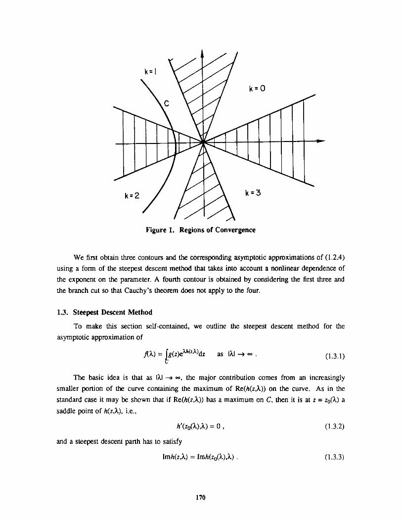
k= I
C
k= 0
3
Figure 1. Regions of Convergence
We first obtain three contours and the corresponding asymptotic approximations of (1.2.4)
using a form of the steepest descent method that takes into account a nonlinear dependence of
the exponent on the parameter. A fourth contour is obtained by considering the first three and
the branch cut so that Cauchy's theorem does not apply to the four.
1.3. Steepest Descent Method
To make this section self-contained, we outline the steepest descent method for the
asymptotic approximation of
fiX) = ig(z)eI(zX)dz as lxi -+ * - (1.3.1)
The basic idea is that as Ill -* oo, the major contribution comes from an increasingly
smaller portion of the curve containing the maximum of Re(h(z,X)) on the curve. As in the
standard case it may be shown that if Re(h(z,X)) has a maximum on C, then it is at z = z0(A) a
saddle point of h(z,X), i.e.,
h'(zO(X),x) = 0 ,
and a steepest descent parth has to satisfy
Imh(z,X) = Imh(zo(X),) .
(1.3.2)
(1.3.3)
170
k='k=2
- fow-T
prr
I I
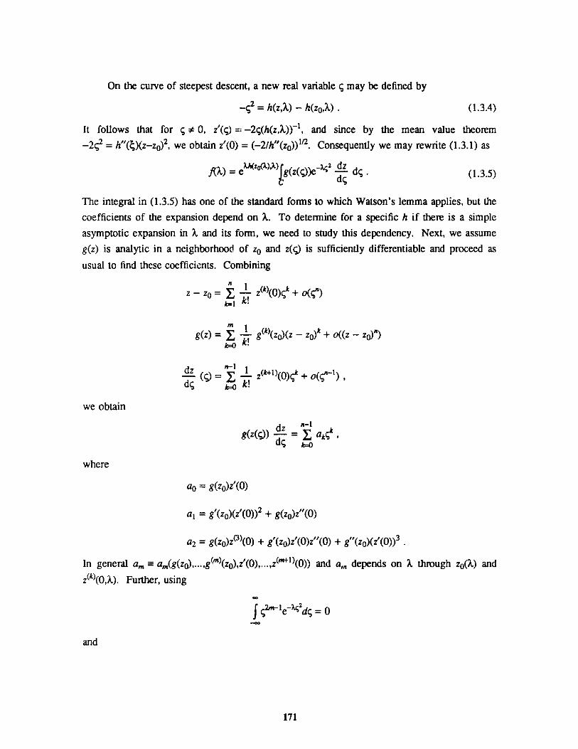
On the curve of steepest descent, a new real variable q may be defined by
-,2 = h(z,)) - h(zo,) . (1.3.4)
It follows that for S 0, z'(g)= -2;(h(z,1))~1, and since by the mean value theorem
-2S2 = h"(|)(z-zo)2, we obtain z'(0) = (-2/h"(zo))2. Consequently we may rewrite (1.3.1) as
fiX) = ezo) g(z())e42 dz d (1.3.5)
The integral in (1.3.5) has one of the standard forms to which Watson's lemma applies, but the
coefficients of the expansion depend on X. To determine for a specific h if there is a simple
asymptotic expansion in ? and its form, we need to study this dependency. Next, we assume
g(z) is analytic in a neighborhood of zo and z(g) is sufficiently differentiable and proceed as
usual to find these coefficients. Combining
z - zo = 1 z(k)(0)q + 1(()
k=1 k!
g(z) = k g(k)(zo)(z - zo)k + o((z - ZO)")k=O
n-1
dz (I) = z(k+ )(0) qk + ( q"~1)
we obtain
n-1
g(z()) dz = I adg ,
where
ao = g(zo)z'(0)
a1 = g'(zo)(z'(0)) 2 + g(zo)z"(0)
a2 = g(zo)z( 3)(0) + g'(zo)z'(0)z"(0) + g"(zo)(z(0))3
In general am= a(g(zo),...,g(m)(zo),z'(0),...,zf"*U)(0)) and a,,, depends on X through zo(X) and
z(k)(0,X). Further, using
J2,n-'e- 2 dg = 0
and
171
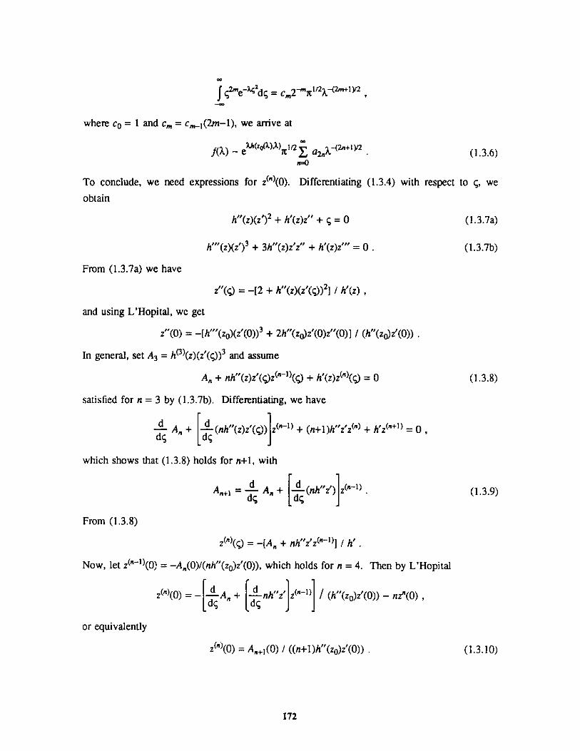
f 2 'ie-Sdg = c,2'"nV2X-(2+'Y2 ,
where co = 1 and cm= c,l_(2m-1), we arrive at
1(X) - e(Z)c1 / a2-2+y (1.3.6),mo
To conclude, we need expressions for z")(0). Differentiating (1.3.4) with respect to q, we
obtain
h"(z)(z')2 + h'(z)z" + g = 0 (1.3.7a)
h'(z)(z')3 + 3h"(z)z'z" + h'(z)z"' = 0 . (1.3.7b)
From (1.3.7a) we have
z"(z) = -[2 + h"(z)(z'()) 2] / h'(z)
and using L'Hopital, we get
z"(0) = -[h"'(zo)(z'(0))3 + 2h"(zo)z'(0)z"(0)] / (h"(zo)z'(0))
In general, set A3 = h 3)(z)(z'(g)) 3 and assume
An + nh"(z)z'()zf"-)() + h'(z)z()(g) = 0 (1.3.8)
satisfied for n = 3 by (1.3.7b). Differentiating, we have
d A + [ (nh"(z)z'(q))1 ~z"~ + (n+1)h"z'zf) + h'z = 0 ,
which shows that (1.3.8) holds for n+1, with
An+1= A + [ (nh"z')]z(n1) . (1.3.9)
From (1.3.8)
z(n)( ) = -[A + nh"z'zt"~1)] / h'
Now, let zf"~1(0) = A (0)/(nh"(zo)z'(0)), which holds for n = 4. Then by L'Hopital
z")(0) = - dA + d[nh"z']z"1)] / (h"(zo)z'(O)) - nz"(O)
or equivalently
zf")(0) = A+ 1 (0) / ((n+1)h"(zo)z'(0)) (1.3.10)
172
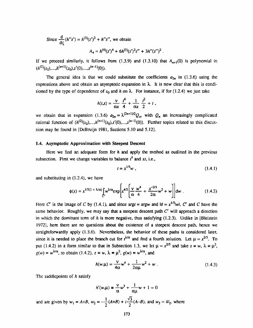
Since -(h"z') = h 3 (z')2 + h"z", we obtaind;
A4 = h(4)(z')4 + 6h(3)(z') 2z" + 3h"(z")2
If we proceed similarly, it follows from (1.3.9) and (1.3.10) that A,, 1(0) is polynomial in
(h(2(zo),...,h("+1)(zo),z'(0),...,z("-1)(0)).
The general idea is that we could substitute the coefficients a2,, in (1.3.6) using the
expressions above and obtain an asymptotic expansion in X. It is now clear that this is condi-
tioned by the type of dependence of zo and h on X. For instance, if for (1.2.4) we just take
vt4 1 t2
h(t,x) = a--- + 2 + t ,
we obtain that in expansion (1.3.6) a2,, = 'an+ly2Q,, with Q,, an increasingly complicated
rational function of (h( 2 (zo),...,h("*0(zo),z'(0),...,z -(0)). Further topics related to this discus-
sion may be found in [DeBruijn 1981, Sections 5.10 and 5.12].
1.4. Asymptotic Approximation with Steepest Descent
Here we find an adequate form for h and apply the method as outlined in the previous
subsection. First we change variables to balance t4 and xt, i.e.,
t = x1/3w , (1.4.1)
and substituting in (1.2.4), we have
4(x) =xl/3(1 +ua))w, aexp x43 v w4 + w2+wdw. (1.4.2)a 4 2a .0
Here C' is the image of C by (1.4.1), and since argt = argw and I-l = xIlwl, C' and C have the
same behavior. Roughly, we may say that a steepest descent path C' will approach a directionin which the dominant term of h is more negative, thus satisfying (1.2.3). Unlike in [Bleistein
1972], here there are no questions about the existence of a steepest descent path, hence we
straightforwardly apply (1.3.6). Nevertheless, the behavior of these paths is considered later,
since it is needed to place the branch cut for tea and find a fourth solution. Let p. = x2. To
put (1.4.2) in a form similar to that in Subsection 1.3, we let p.= x2 and take z = w, A = 2,
g(w) = wu, to obtain (1.4.2), z = w,X= 2 ,,g(w w ,and
h(w,)=-)_-w4 + w2+w .(1.4.3)4a 2a
The saddlepoints of h satisfy
h'(w, ) = -- w + w+ 1 = 0a a
and are given by w1 = A+B, w2 = -- (A+B) + i-(A-B), and w3 = W2, where2 2
173
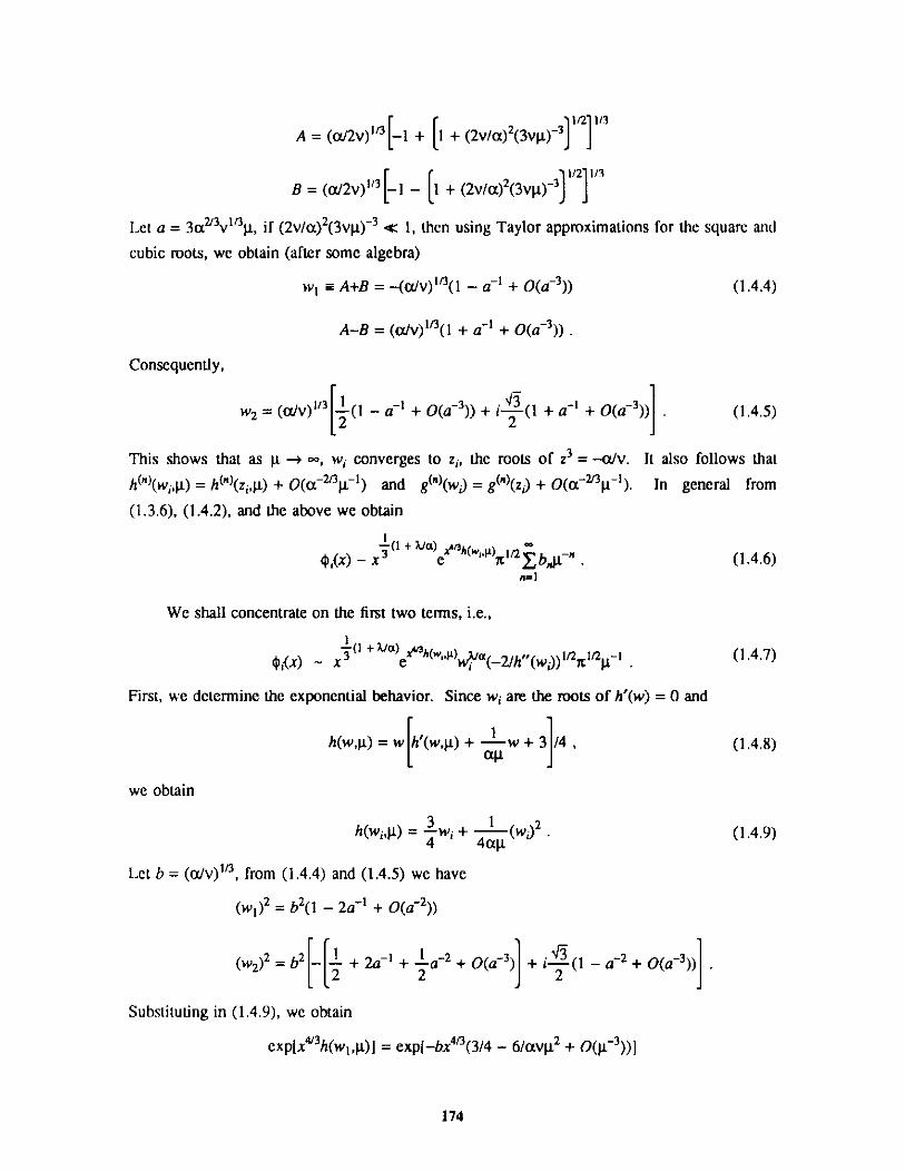
1/2 1/3
A = (a/2v)"3 [-1 + 1 + (2v/Q)2(3v )~3
B = (/2v)"' 3 -1 - 1 + (2v/a)2(3vp)~3
Let a = 3a 3v"3 p, if (2v/a) 2 (3v )-3 < 1, then using Taylor approximations for the square and
cubic roots, we obtain (after some algebra)
w, =A+B = -(a/v) 1 /3(l - a' + O(a-3)) (1.4.4)
A-B = (a/v)1' 3 (1 + a-' + O(a~3)) .
Consequently,
w2 = (a/v)E/3 2[( - a 1 + 0 ~3))+ 2(1+ a + O -3)) . (1.4.5)2 2
This shows that as -+ oo, w; converges to z, the roots of z3 = --a/v. It also follows that
h0")(w;, ) = h(")(z;, ) + O(a-2 3 -') and g(")(w) = g(")(z) + O(~2/3p- 1). In general from
(1.3.6), (1.4.2), and the above we obtain
-(1 + 7Va) p0
$1(x)a)x e ' n bs~". (1.4.6)n=1
We shall concentrate on the first two terms, i.e.,
$;(x) ~_ x 3 +je h(w-) a_2/h"(w; ~ .- (1.4.7)
First, we determine the exponential behavior. Since w are the roots of h'(w) = 0 and
h(w, ) = w h'(w,) +1w + 3]/4 , (1.4.8)
we obtain
h(w,) w+ (w) 2 . (1.4.9)4 4ajg
Let b = (a/v)"3 , from (1.4.4) and (1.4.5) we have
(w1)2 = b2(1 - 2a' + 0(a~2))
(w2)2 = b2[_[i + 2a~1 + a-2 + O(a~3) + i (1 - a-2 + O(a-3))]2 2 2
Substituting in (1.4.9), we obtain
exp[x 413 h(w1 ,)] = exp[-bx413(3/4 - 6/avp 2 + O( -3))1
174
exp[x4/3h(w2,4)] = exp[bx4'3((3/8 - 3/(8a) + O(a-2 )) + i( + /2+ /(4a) - O(a~3)))]
In a similar fashion we have
h"(w1,p) = 3b(1 - a-' + O(a-2 ))
h"(w2, ) = 3b - 1 - a-' + O(a2) + i4(1 + O(a-2))
Let p = ReA/a and q = ImX/c. Using the linear approximation for tan(arg(w;)), we obtain
w3 a = (b - ba-1 + O(~3))'exp{qic + i[q(b - ba~1 + O(a 3 )) - pi]}
]bw3a = b - ba-1 + O(a2) exI{-q(n/3 + 4l/(2a) + O(a-2 ))
+ i q(b + jba' + O(a-2)) + p(n/3 + I/(2a) + O(a-2))].
The expressions for w3 are the conjugate of the expressions for w 2, except in w3 where the
whole exponent is multiplied by -1.
1.5. Steepest Descent Paths
In this subsection we briefly describe the behavior of the steepest descent paths which is
needed to place the branch cut and determine a fourth solution. Let w = u+iv. From (1.4.3)
we have
Reh(w, ) = --- (u4 + v4 - 6u2v 2) + - (u2-v 2) + u (1.5.1)4a 2cqs
Jmh(wp) = KYuv(u2 - v 2) + I-uv + v . (1.5.2)a a
Since w1 is real, the path through w1 satisfies Imh(w,) = 0, i.e.,
v u(u2_v2) + -1-u+ 1 = 0. (1.5.3)a a
The curve v - 0 is of steepest ascent. This follows by substituting in (1.5.1) and observing
that w 1 is a minimum of Reh(w, )Ia. Hence, the term in brackets in (1.5.3) is zero, and the
path is given by
v(u) = (u2 + (v )-1 + oc/(vu))Ia2, u 5 w1 . (1.5.4)
From (1.5.4) it follows that as u -* -oc, Iv(u)I 4 luI and arg(w) converges to 3/4 or 5/4.
175
Next, we consider the paths through w 2 and w3. Let a = Imh(w2 ,). From (1.3.3) and
(1.5.2) we obtain that the path through w 2 satisfies
uv3 - (u3 + (u/vp) + o/v)v + aa/v = 0 (1.5.5a)
v3 - (u2 + (v )1 + (W/vu))v + (cza/vu) = 0 . (1.5.5b)
Notice that if (u,v) satisfies (1.5.5), then (u,-v) satisfies (1.5.5) with a substituted by
-a a Imh(w 3,p). In other words, if (u,v(u)) is the steepest descent path through w2 , then
(u,-v(u)) is the path through w3. Hence we concentrate on the former.
Let s = (u2/3 + (3v )-1 + (a/3vu))1 and k = -(aa/2vu)/s 3. The roots of (1.5.5) are
vi(u) = C + D , v2(u) = -(C+D)/2 + i(4 /2XC-D) , v3(u) =v~2(u) , (1.5.6a)
where
C = s(k + (k2-1)" 2)'/3 , D = s(k - (k2-1) 2 )"3. (1.5.6b)
If k > 1, v1(u) is the only real solution, and if k2 < 1, there are three real solutions given by
v(u) = 2s cos (/3 + 2(-1)x/3) , I = 1,2,3 , (1.5.7a)
where $ satisfies
cos $ = k. (1.5.7b)
Conceder first the case u 0. Since k2 > 1 is equivalent to (aa/2v)2 > u2s6 and the
minimum of u2s6 is (aa/2v)2, attained at u = Re(w2), we have that k 2 < 1, except at u = Re(w2)
where k2 = 1. Consequently, we have to consider the behavior of the three solutions (1.5.7).
When lul - , ka -a/(2vulul 3 ), and if u 1 0, k - -a(3vu/2x)"2. Hence from (1.5.7b),
* -+ x/2; and using the linear approximation for cost$, we obtain $/3 - x/6 - h/3. Conse-
quently, from (1.5.7a), using Taylor expansions, we have
v1(u) - 4Is + sk/3 + O(sk2) (1.5.8a)
v2(u) -4IUs + sk/3 + O(sk2) (1.5.8b)
v3(u) ~ -2sk13 + O(sk2) . (1.5.8c)
As IuI -+ a, sk -+ 0 and '3s = Iul(1 + (vpu2'-1 + (a/vu3 ))I". Also, as u 1 0, sk -+ -3a/2 and
,s - (x/vu) 1V
2. It follows that for w = u + iv1(u), arg(w) -+ x/4 as u -+ W and
arg(w) -+ 3x/4 as u - - , while arg(w) -+ i/2 as u 0. For u = 0, v3(u) = a, which satisfies
(1.5.5a).
In the neighborhood of u = Re(w2) we have that as u -+ Re(w2), k -+ -1. Consequently,
* -+ it. From the Taylor expansion of cos$ we obtain * ~ iS, where = (2+2k)1l2
Hence,
176
vl(u) - s(1 T 4 3&3 + 0(62)) >O0
v2(u) - s(-2 + 0(62)) < 0
V 3() ~ s(l 4 &3 +0(82)) > 0 .
Notice that v1(u) and v2(u) are discontinuous since v1(Re(w2)) < 0 and v2(Re(w2)) > 0.
Next we consider the case u < 0. When u T 0, making the change of variables x = -u,we obtain
C = s(k + (l+k2)la')l 3 , D = s(k - (I+k2):0,1/3
where s = (aW3vx - x2/3 - (3v )~')lt2 and k = aa/(2vxs 3). Since k - (3a/2X3vx/A.)" 2 , v1(u) is
the only real solution. Arguing as before, we obtain
vl(u) = s(2k/3 + 0(k3)).
Hence, as x410, k - 0, and v(u) -4a. Finally, let uo < 0 be such that k2 = 1 in (1.5.6b). As
u T uo, we have the solutions (1.5.7a), and since k T 1 from (1.5.7b), it follows that
(2-2k)'I and
v1(u) ~ s(2 - O(1-k))
v2(u) ~ s(-1 + 0((1-k)1a))
v3(u) ~ s(-1 - 0((1-k)la))which shows that v2(u) < 0, v3(u) < 0, and v1(u) continuous at uO.
In conclusion, we have that the steepest descent through w2 is given by
(i) (u,v 1(u)) for -oo < u < 0 and Re(w2) < u < +oo
(ii) (u,v3 (u)) for 0 5 u 5 Re(w2) .
Pictorially,
177
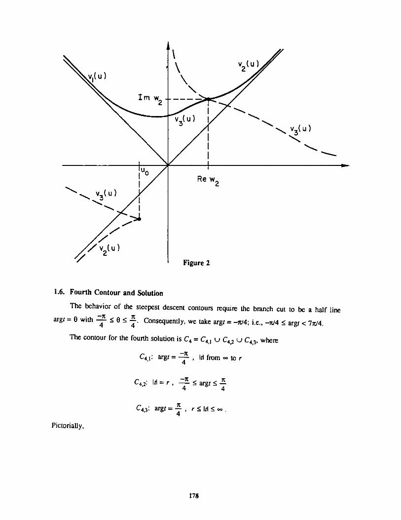
Im(u)
I 2
u
v(u)
3 I
/v 2(u)
v v (uv (U3
1 I I lwRe w
Figure 2
1.6. Fourth Contour and Solution
The behavior of the steepest descent contours require the branch cut to be a half lineargt = 0 with S 805 - . Consequently, we take argt = -c/4; i.e., -/4 5 arg <7/4.
4The=contir 4s,,, whe <
The contour for the fourth solution is C4 = C4,1 U C4,2 U C43, where
C4,1: argt =2= , Id from oo to r4
C4,2: Idl=r, ~- argt4 4
C4,3: argt=- -, r Idl c.4
Pictorially,
178
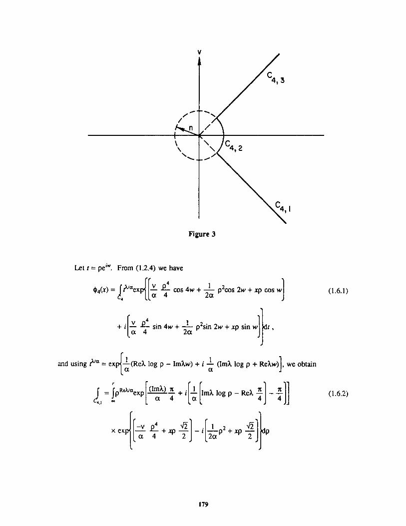
V
C4, 3
C
44,,2
C4,
Figure 3
Let t = pei"'. From (1.2.4) we have
4
$4= JA/ae ?"xp{ _ cos 4w + -- p2cos 2w + xp cos w (1.6.1)
44
+ i -- sin 4w + 1 p2sin 2w + xp sin wdt ,a 4 2a
and using thA = expfi(RcX log p - Imkw) + i (Implog p + Rekw) we obtain
r
= fpRehexpFm + ixImp log p - Red, - (1.6.2)4+ a 4 a 4 4
x ex - + xp-N - - Ip2+ xp - pa 4 2 2a 2
179
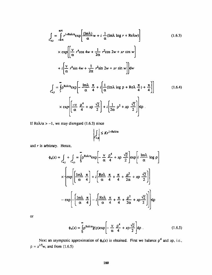
L/4
= r+R Imex ) 1 w + i (Imp log r + Rekw) (1.6.3)-4 V -XP/
x ex {[ r4 cos 4w + r2cos 2w + xr cos w6 26
+ i rosin 4w + 2 r2sin 2w + xr sin w wa 4 2a
=JpReaexp Im . + i 1(Im log p + Re. l ) + I (1.6.4)4,XLa 4 ab 4 4JJ
x ex ~ i+xp ] + i[ p2+xp -2]dpa 4 2 2a 2
If Rea/a > -1, we may disregard (1.6.3) since
SKrl+RWja
and r is arbitrary. Hence,
4 4(x)=J + = pRe/aexp [-v + xp exp i log p41 4.3 . a 4 2 a
x exp Imp,- +i +n +xp ,2a 4 a 4 4 2a 2
- exp- Imp, n _ Red n + n+ 2+ xp pa 4 a 4 4 2a+ 2
or
$4(x) = pRa+(p)expx-P dp. (1.6.5)a 4 2
Next an asymptotic approximation of $4(x) is obtained. First we balance p4 and xp, i.e.,
p = x11 w, and from (1.6.5)
180
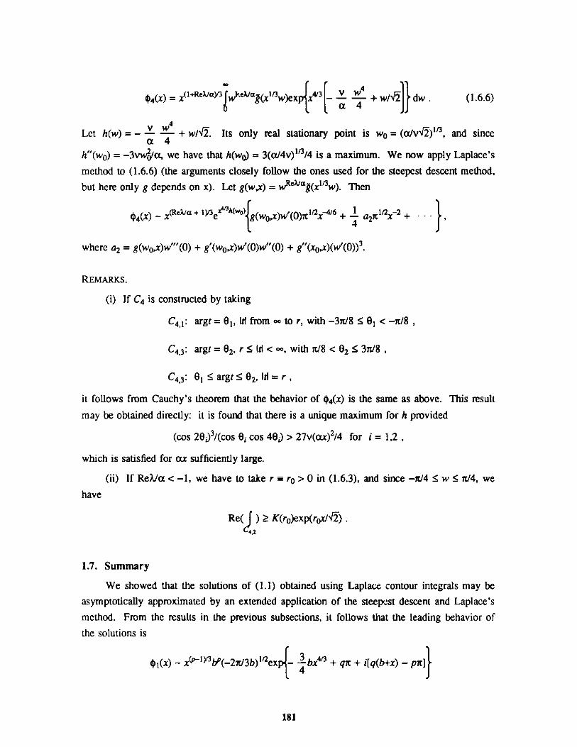
44(x) = x(1+Rea)3 .e)/ag(x1x3w)exx4/3 -v . + wj dw . (1.6.6)
Let h(w)= - + w/4. Its only real stationary point is wo = (a/v41)'S, and since(X4
h"(wo) = -3vw4/a, we have that h(wo) = 3(/4v)"3 /4 is a maximum. We now apply Laplace's
method to (1.6.6) (the arguments closely follow the ones used for the steepest descent method,
but here only g depends on x). Let g(w,x) = wRea(x 1/3w). Then
0 4(x) x ' + 1)3e (wo) g(wox)w(0)7c /2x-/ 6 + I a2 C1x2- 2 + - ii
where a2 = g(wo,x)w"'(0) + g'(w0,x)w'(0)w"(0) + g"(xo,x)(w'(0))3
REMARKS.
(i) If C4 is constructed by taking
C4 ,1: argt = 01, Idtfromcoo to r, with -3i/8 5 01 < -/8 ,
C4,3: argt = 02 , r Sld<oo, with i/8 <02 53ic/8,
C4,3: 01 5 argt 5 02, Id = r,
it follows from Cauchy's theorem that the behavior of $4(x) is the same as above. This result
may be obtained directly: it is found that there is a unique maximum for h provided
(cos 20;)3/(cos 0; cos 40;) > 27v(ax)2 /4 for i = 1,2 ,
which is satisfied for ox sufficiently large.
(ii) If ReA/a < -1, we have to take r = ro > 0 in (1.6.3), and since -x/4 5 w : 5i/4, we
have
R() z K(ro)exp(rax/n).
4.2
1.7. Summary
We showed that the solutions of (1.1) obtained using Laplace contour integrals may be
asymptotically approximated by an extended application of the steepest descent and Laplace's
method. From the results in the previous subsections, it follows that the leading behavior of
the solutions is
$5(x) - x(P-1Yb(-2cJ/3b)1r2exp - -bx4/3 + qp + i[q(b+x) - px]
181
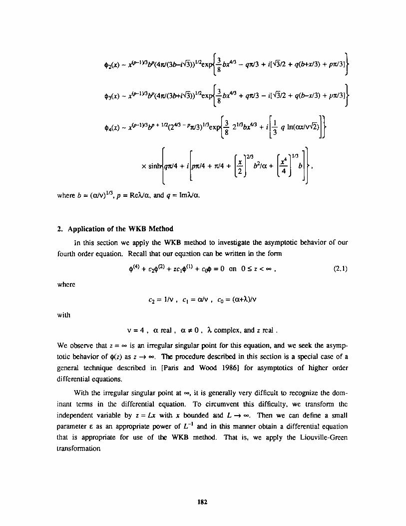
$ 2 (x) - x(P1b(41/(3b-i r-))1f2ex { bx4f3 - qi/3 + i[43/2 + q(b+x/3) + px/31}
$3(x)- x1Y b(47J(3b+i1))Iexpibx4r3 + gi/3 - i[1/2 + q(b-x/3) + pn/3]
$4(x) ~ x" l~Mb" + 1/2(24/3 - P 3)1I3ex p{ 21 3 bx4 + i q ln(ax/v)
0 42A 41/
x sinh{q /4 + i pit/4 + n/4 + -]b2/a + [ib]
where b = (a/v)1 3 , p = ReX/a, and q = ImX/a.
2. Application of the WKB Method
In this section we apply the WKB method to investigate the asymptotic behavior of our
fourth order equation. Recall that our equation can be written in the form
$(4)+c2 (2 )+zc 1 (1+co$ = 0 on05z<oo, (2.1)
where
c2 = 1/v , c1 = a/v , co = (a+?,)/v
with
v=4 , areal, a O0 , complex, and z real .
We observe that z = oo is an irregular singular point for this equation, and we seek the asymp-
totic behavior of $(z) as z -+ oo. The procedure described in this section is a special case of a
general technique described in [Paris and Wood 1986] for asymptotics of higher order
differential equations.
With the irregular singular point at oo, it is generally very difficult to recognize the dom-
inant terms in the differential equation. To circumvent this difficulty, we transform the
independent variable by z = Lx with x bounded and L -+ 0. Then we can define a small
parameter E as an appropriate power of L-1 and in this manner obtain a differential equation
that is appropriate for use of the WKB method. That is, we apply the Liouville-Green
transformation
182
y(x) = ex{ S(x;E)},
expand S(x;E) in an asymptotic series in e, and calculate successive terms until we achieve
algebraic behavior. In this manner we expect to determine the leading behavior of each
independent solution of $ as z -4 oo.
We start by setting
z=Lx, 05x5 1 , O<L-oo (2.2)
and
u(x;L) = 4)(z) . (2.3)
The differential equation takes the form
L-4u( + L-2c2u2 + xc1L-7u( 1) + c 0L~4u = 0 . (2.4)
At this point we do not know the appropriate power of L1 to use as our small parameter E.
There are two stages and two parameters involved in this procedure. We first want to have thehighest power of E multiplying the highest derivative which is appropriate for applying the
Liouville-Green transform. Then we need another free parameter in order to balance terms in
the transformed equation. To this end we divide (2.4) by L~4 and set e = L4, where y and S
will be selected presently. We find
E 6 U(4) + E 8 C2u()+ xc1 +U(1)+ C =0-(2.5)
To achieve the desired form E4u(4) +... = 0, we choose =X 4, which yields
42 4 44
E4) + C2E aU() + xCE u1)+ Coe 8u = 0 . (2.6)
We now apply the Liouville-Green transformation u(x) = exP i S(x)}.
E3S( + E2[4S'S11 + 3(S")2] + 6E(S') 2S" + (S')4 (2.7)
4-2-1 4--2 4-4-1 4-4+ C2E 8 nS" + C2E S (S')2 + XC 1E 6 S,+ CDE =
We observe that the term (S')4 is 0(1), and we choose S in order to balance this term against4-1
the largest of the other terms. If we balance against the xc1E SS' term, then the remain-
ing terms will be higher powers of e. To this end we select S = 4/3, which gives y = 4/3.
With this choice the equation for S takes the form
183
(S')4 + sc1S' + c2E" 2 (S') 2 + Eico + 6(S')2SP] + E3/2 n
+ E2 (4S',S + 3(S")21] + E3S(4) =0.(2.8)
Considering the fractional powers of E, the natural expansion for S(x;E) would be
S(x;e) = So(x) + E'r2Ro(x) + eS1(x) + E3RR(x) + E2S2(x) +... . (2.9)
With this expansion in (2.8) we have the following equations for each order.
0(1): (Eikonol equation)
(S'O)4 + xc1S'o = 0 (2.10)
O(E1/2):
[4(S'O)3 + xci]R'o + c2(S'0)2 = 0 (2.11)
D(E):
[4(S'0)3 + xc1]S'1 + 6(S'0)2(R'0)2 + 2c2 S'oR'o + 6(S'o)2S"o + co = 0 . (2.12)
Starting with the Eikonol equation we consider first the case when
S'o #0. (2.13)
In this case (2.10) has the form
Recall that c1 = a/v. We distinguish two cases a < 0. For k = 1,2,3 define
exp 13 (2k-1) , if a> 0
Pk- -(2.14)exp.2 k] , ifa<0
These complex cube roots are as shown in Figure 4.
184
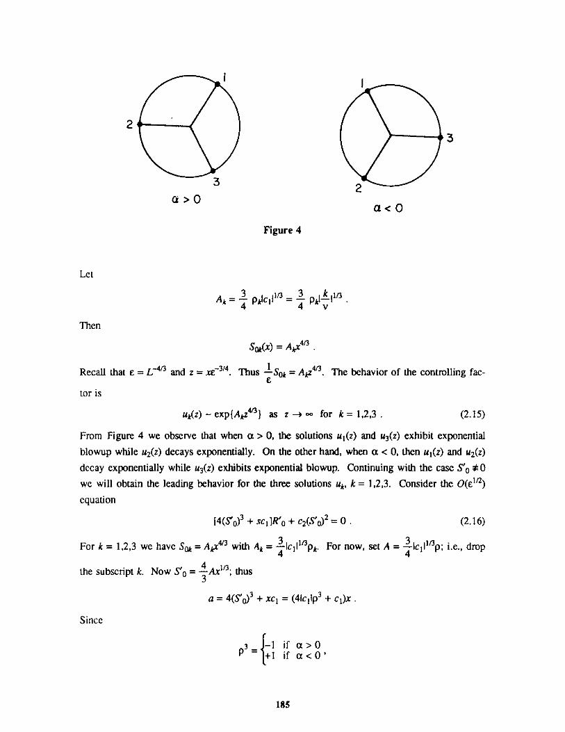
2
3
ci>0
3
2
a<0
Figure 4
Let
Ak = 3Pk cilin = 3 pl!I11/34 4 v
Then
So(x) = Akx 413 .
Recall that e = L~4/ and z = xE3/4. Thus 1 Sok = Az 4 . The behavior of the controlling fac-
tor is
Uk(Z) - exp(Akz"'} as z -+ o for k = 1,2,3 . (2.15)
From Figure 4 we observe that when a > 0, the solutions u1 (z) and u3 (z) exhibit exponential
blowup while u2(z) decays exponentially. On the other hand, when a < 0, then u1 (z) and u2(z)
decay exponentially while u3(z) exhibits exponential blowup. Continuing with the case S'0i k0we will obtain the leading behavior for the three solutions Uk, k = 1,2,3. Consider the O(EIa)
equation
[4(S'o)3 + sci]R'o + c2(S' 0)2 = 0 (2.16)
For k = 1,2,3 we have S_= A 43 with 4= k= Ic4lcpP. For now, set A = ,IclIap; i.e., drop
the subscript k. Now S'o = 4Ax'; thus3
a = 4(S'o)3 + xc1 = (41c11p3 + c1)x .
Since
P3 = -lS ~+l
if a> 0if a < 0'
185
we find a = -3xc 1 in either case. Equation (2.16) takes the form
-3xc1R'0 + 91 c2A2x2r3= 0, A = Ak.9
Let
1 IcI 2Bk =-c2 pc12 , k = 1,2,3. (2.17)2 c1
Observe that when a > 0 we have Re(B 1 ),Re(B 3 ) < 0 while Re(B 2) > 0, lm(B2) = 0, whereas
for a < 0 we have Re(B1),Re(B2) > 0 with Re(B3) < 0, Im(B3) = 0. The solution of (2.16) is
Rok(x) = Bkx2 3 for k = 1,2,3.
In terms of z this gives
Rok(z) = ElzBkz2n
Thus far we have
uk(z) ~-exP{ Sok +-Ro + - }-- = exPAkz43 + Bkz2J3+ - }-.-, z -+ oo .
To determine whether we have the leading behavior and to display the dependence on X, we
will proceed to the next order.
At 0(e) we have (for the case S'0 * 0)
[4(S'0)3 + xc1 ]S'1 + 6(S'0)2(R'0)2 + 2c2 S'oR'o + 67(S'0)2S"o + co = 0
To evaluate the terms in this equation, we drop the k subscript so that So = Ax4d3 and
Ro = Bx21 3. Then
6(S'0)2(R'o)2 9234 A 2B2x 0
c2 42
2c2SoR'0 = ABx0
6(5')25.0= 2-3.43 A 3x0
92
CO = co 9 .
Thus
2--3 3c2A BDk = A + 24 [A + + AB , k = 1,2,3 , (2.18)
and the equation for S1(x) takes the form
186
-3xc 1 S'1 + D = 0,
so that
Di
SIk(x)= --cnx . (2.19)3c1
With SIk(x) we have algebraic behavior for uk(z) so that we now have the leading behavior in
Uk(X) for k = 1,2,3. We have
uk(z) -z '3c'exp(Az 4 13 + Bkz" + - ) as z -+ co. (2.20)
Before going on we simplify the expression for Dk. Using the definitions of Ak, Bk, and Pk, we
find that D is independent of k and in fact
Dk wD = (X - a)/v (2.21)
which is real when ? is real. To check that negative powers of z appear in the exponential at
the next order, we will solve for the next order.
The equation at O(E3/2) is
-3xc 1R'1 + 8(S' 0)2S' 1R'0 + 2S' (R'0 )3 + 2c2S'0S'1 + c2(R' )2 + 6 S')2R"
+ 12S'oS"oR'o + c2S" 0 = 0 . (2.22)
With
S'0 = Ax t, S~ = AAx3,3 9
R'0 = 2 Bx-3 , R"o = - 2 Bx 3 , S'1 = D/3c1x ,3 9
we find that (2.22) takes the form
-3xc 1R'1 + Ex~ 3 = 0,
where
162 A2DB 82 3 84 2 43 4E=- D +-AB +-c 2AD+-c2B +2-A2B+-c2 (2.23)92 c1 33 9 9 33 9
We find
R E=- x~3=-E-112E z~"a
2c1 2c1
Thus
187
uk(z) ~-z cex A z +B-z2 _- cz-2 +... as z -+ co-for k = 1,2,3 .2ci
That is,
Uk(Z) ~ z-3-z3exp 3 pkI-I13z4/3 + 1 2 3z + + -- (2.24)4 v 2 a v
as z-*40 for k = 1,2,3,
where Pk is defined in (2.14). We now have the leading behavior for the three independent
solutions {uk: k = 1,2,3}. These solutions arose in the case when S'o 40. We now consider
the case when S'0 = 0, which will generate the fourth solution uo(z). Since S'0 = 0, it would be
natural to try the expansion
u(x) ~ exp(T1 (x) + E1/2F1 (x) + ET2(x) + E32F2(x) +...} (2.25)
in (2.6). Recall that S = 4/3; thus (2.6) reads
E4u 4 + tEcXu + Ecou + E5/202) = 0 . (2.26)
With the expansion (2.25), we find the following equations at each order:
0(c): xc1 T 1 + co = 0
O(E3/2): xc1 F'1 = 0
0(E2 ): xc 1 ' 2 = 0
O(E512 ): xc1 F'2 + c2(" 1 + (T 1)2 ) = 0 .
Solving these equations, we find
CoT(x)=-- lnx = - (1 + -)lnx
cl a
SC2 Co C0F2(x) 2= C-O- (1 + -)x-2 = -(1 + -)(2 +-)2
2 c 1 c c 2a a a
Now z = xe-314 so that E3/2 -2 = z 2 , and we find
u ((z)-~ z ( aex -- (1 + -)(2 + -.)z~2 +... as z (2.26)2a a a
We can summarize the results of this section as follows. We have found the leading behavior
as z -+ 00 for the four independent solutions of (2.1). There are two cases to consider.
CASE 1. a>0
188
In this case two solutions u1(z), u3 (z) exhibit exponential blowup with oscillations for
all values of X. The third solution u2(z) exhibits exponential decay of nonoscillatory
type for all values of X. The fourth solution u0(z) has algebraic behavior as z -+
with u0 (z) going to zero where Re(?) > -a.
CASE 2. a <0
In this case two solutions u1 (z) and u2(z) exhibit exponential decay with oscillations for
all values of X. The third solution u3 (z) exhibits exponential blowup with the control-
ling factor nonoscillatory. The fourth solution u0(z) has algebraic behavior with u0(z)
going to zero when Re(k) > -a.
We now consider the case where a = 0 in which case c1 = 0 and c0 = AJv. Equation
(2.7) has the form
E3S(4) + E2[4S'S" + 3(S")2] + 6E(S') 2S" + (S')4
2 2 4
+ c2E-S" + C2E -(S)2 + coE = . (2.27)
Balancing the 0(1) term against the largest of the other terms, we find 5 = I which yields
(S') 4 + c2(S')2 + co + e[c2 S" + 6(S')2S"1 + E2[4s'SPI' + 3(S")2] + E30(4) . (2.28)
With S = 1 we have y = 0, e = L~1, and x = Ez. Recall that the Liouville-Green transformation
m as used to obtain the S equations, i.e.,
u(x) = exp{- S(x;E))E
Considering the powers of E appearing in (2.28), it would be natural to try the following
expansion for S(x;E).
S(x;E) = So(x) + ES1(x) + e 2S2 (x) +--- . (2.29)
We find the following equations at each order:
O(1): (S'0)4 + c 2 (S'0)2 + c0 = 0
O(E): [4(S'0)3 + 2c2S'o]S'1 + c 2S" 0 + 6(S'o) 2S"o = 0
0(0): [4(S'0)3 + 2c2 S 0]S'2 + 6(S'0)2(S'1)2 + c2 (S 1 )2 + c2 S"1 + 12S'S'1S"0
+ 6(S'o)2S" 1 + 4S'oS"' 0 + 3(S" 0)2 = 0 .
When a = 0, we will restrict a to be real. Consider the 0(1) equation. Since c2 = -,V
189
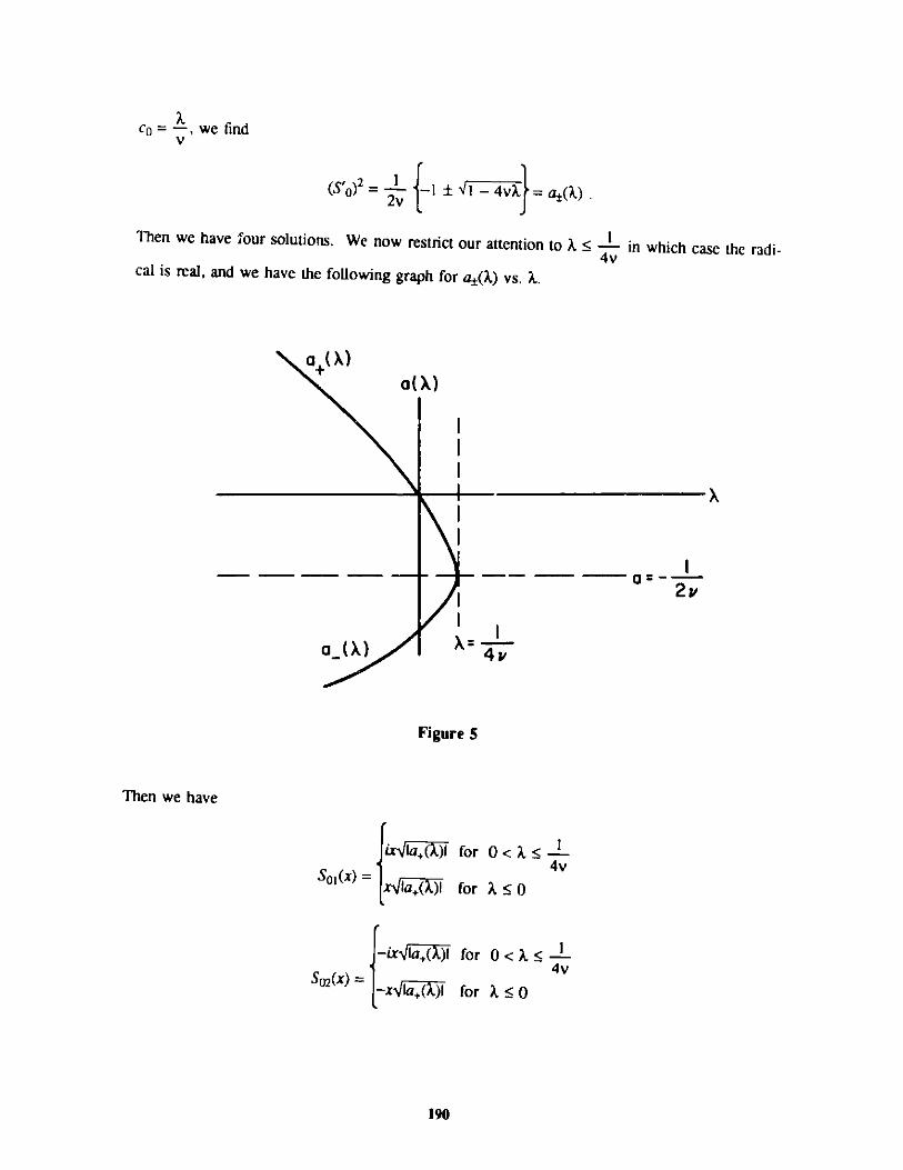
co= -, we findv
(S'0 )2 =L{-1 l- v ay(X) .
Then we have four solutions. We now restrict our attention to X S in which case the radi-4v
cal is real, and we have the following graph for at(),) vs. )1.
a+(X)a(X)
a_(X)
x
2v
-4v:
Figure 5
Then we have
ix[la+(V)I for 0 < 1I 4V
Sol(x) = 4
( +(xi()l for X 5 0
-ixF la+(I) for 0 < L5-I4v
So2(x) =-x la+( )I for 7l S 0
190
i
i
i
S03(x) = ixIa_()I for A 44v
S04(x) = -ix Jla_( ) for X .
4v
Thus we observe that for 0 < A 5 1/4v the four solutions S(x;,) are pure imaginary.
Consider the O(E) equation. In this equation we have the coefficient
fi = 4(S'o)3 + 2c2S'o = S'0(4(S'o)2 + 1) = ( 241 - 4vX)S'0 ,V V
and so we see that fl 0 where A < . Since So(x) are linear in x, we see that the O(E)4v
equation has the form
S'o(x)(k2 41 - 4vX)S'1(x) = 0V
which gives S1(x) = 0. In a similar manner we find S2(x) = 0. Thus we expect that the
behavior at infinity is governed by the behavior of the four solutions given above. Thus we
find for a = 0 the following behavior at infinity:
uk(z) - exp(zek(A)) , k = 1,2,3,4 as z -4 oo,
where
i ia()I for 0 < A <4V
e1()l=a+( ) for A S0
e2(A) = -e 1(A)
e3 (A)iI4a_()I
e4(A)= -e3 (A)
References
N. Bleistein and R. A. Handelsman 1972. "A generalization of the method of steepest des-cent," J. Inst. Math. Applic. 10, 211-230.
G. F. Carrier, M. Krook, and C. E. Pearson 1966. Functions of a Complex Variable,McGraw-Hill, New York.
E. T. Copson 1965. Asymptotic Expansions, Cambridge University Press, Cambridge.
191
N. G. DeBruijn 1981. Asymptotic Methods in Analysis, Dover Publications, New York.
H. G. Kaper and B. Schultze 1988. "Spectral analysis of a fourth-order singular differentialoperator," Proc. 1986-87 Focused Research Program on "Spectral Theory and BoundaryValue Problems," ANL-87-26, Vol. 2, Hans G. Kaper, Man Kam Kwong, and Anton Zetti
(eds.), Argonne National Laboratory, Argonne, Illinois.
J. D. Murray 1984. "Asymptotic analysis," Applied Mathematical Sciences, Vol. 48,Springer-Verlag, New York.
R. B. Paris and A. D. Wood 1986. Asymptotics of High Order Differential Equations, Long-man Scientific & Technical, Harlow, Essex, U.K.
A. L. Rabenstein 1958. "Asymptotic solutions of u ' + X2(zu" + cu' + Du) = 0 for large IXI,"Arch. Rational Mech. Analysis 1, 418-435.
G. I. Sivashinsky, C. K. Law, and G. Joulin 1982. "On stability of premixed flames instagnation-point flow," Combustion Science and Technology 28, 155-159.
W. Wasow 1965. Asymptotic Expansions for Ordinary Differential Equations, IntersciencePublishers, New York.
192
Distribution for ANL-87-26, Vol. 2
Internal:
J. M. Beumer (3)F. Y. FradinM. GarbeyH. G. Kaper (30)A. B. KrisciunasM. K. KwongG. W. Pieper (30)
ANL Patent DepartmentANL Contract FileANL LibrariesTIS Files (3)
External:
DOE-OSTI, for distribution per UC-405 (66)Manager, Chicago Operations Office, DOEMathematics and Computer Science Division Review Committee:
J. L. Bona, Pennsylvania State UniversityT. L. Brown, University of Illinois, UrbanaP. Concus, Lawrence Berkeley LaboratoryS. Gerhart, Micro Electronics and Computer Technology Corp., Austin, TXH. B. Keller, California Institute of TechnologyJ. A. Nohel, University of Wisconsin, MadisonM. J. O'Donnell, University of Chicago
W. Allegretto, U. of Alberta, CanadaF. V. Atkinson, U. of Toronto, CanadaD. Austin, ER-DOEP. Bailey, Sandia National LaboratoriesChr. Bennewitz, U. of Uppsala, SwedenH. Benzinger, U. of IllinoisR. C. Brown, U. of AlabamaA. Castro, North Texas State U.C. Y. Chan, U. of Southwestern LouisianaS. Chen, Shandong U., People's Republic of ChinaL. Erbe, U. of Alberta, CanadaW. N. Everitt, U. of Birmingham, U.K.C. T. Fulton, Florida Inst. of TechnologyJ. Goldstein, Tulane U.G. Halvorsen, Inst. for Energy Technology, NorwayB. J. Harris, Northern Illinois U.D. Hinton, U. of TennesseeV. Jurdjevic, U. of Toronto, CanadaA. M. Krall, Pennsylvania State U.G. Michael, Lawrence Livermore LaboratoryA. B. Mingarelli, U. of Ottawa, Canada
- 193 -
J. Neuberger, North Texas State U.S. Pruess, Colorado School of MinesT. Read, Western Washington U.J. Ridenhour, Utah State U.B. Schultze, U. Gesamthochschule Essen, West GermanyG. Sell, U. of MinnesotaJ. Serrin, U. of MinnesotaJ. K. Shaw, Virginia Polytechnic inst. and State U.E. Socolovsky, U. of PittsburghL. Veron, Universite Tours, FranceA. Zettl, Northern Illinois U.
- 194 -