Embed Size (px)
Citation preview
NOVEMBER 2004 2413B A N A S E T A L .
q 2004 American Meteorological Society
Dynamics of Willapa Bay, Washington: A Highly Unsteady, Partially Mixed Estuary
N. S. BANAS, B. M. HICKEY, AND P. MACCREADY
School of Oceanography, University of Washington, Seattle, Washington
J. A. NEWTON
School of Oceanography, University of Washington, Seattle, and Environmental Assessment Program,Washington State Department of Ecology, Olympia, Washington
(Manuscript received 24 February 2003, in final form 4 May 2004)
ABSTRACT
Results from 3 yr of hydrographic time series are shown for Willapa Bay, Washington, a macrotidal, partiallymixed estuary whose river and ocean end members are both highly variable. Fluctuating ocean conditions—alternations between wind-driven upwelling and downwelling, and intrusions of the buoyant Columbia Riverplume—are shown to force order-of-magnitude changes in salinity gradients on the event (2–10 day) scale. Aneffective horizontal diffusivity parameterizing all up-estuary salt flux is calculated as a function of riverflow:results show that Willapa’s volume-integrated salt balance is almost always far from equilibrium. At very highriverflows (the top 15% of observations) the estuary loses salt, on average, while at all other riverflow levelsit gains salt. Under summer, low-riverflow conditions, in fact, the effective diffusivity K is large enough to drivea net increase in salinity that is 3–6 times the seaward, river-driven salt flux. This diffusion process is amplified,not damped, by increased tidal forcing, contrary to the expectation for baroclinic exchange. Furthermore, Kvaries along the length of the estuary as ;5% of the rms tidal velocity times channel width, a scaling consistentwith density-independent stirring by tidal residuals. To summarize Willapa’s event- and seasonal-scale variability,a simple diagnostic parameter space for unsteady estuarine salt balances is presented, a generalization from theHansen and Rattray steady-state scheme.
1. Introduction
This paper examines the net fluxes of salt in and outof Willapa Bay, Washington, on event (2–10 day) andseasonal time scales. Willapa is a coastal-plain estuaryconnected to a highly active eastern boundary ocean,the northern reach of the California Current System(Hickey 1989). The interest of salt dynamics in thisestuary is on one level regional and ultimately ecolog-ical, while at the same time is tied to a general, theo-retical concern: the often-neglected role of time-depen-dence in estuarine dynamics and classification.
Analytical theories of estuarine circulation over-whelmingly rely upon the assumption of a steady stateto reach tractable solutions. The classical core of thisfield is the analytical solution of Hansen and Rattray(1965), hereinafter HR65, and the closely related di-agnostic scheme of Hansen and Rattray (1966), here-inafter HR66. The HR66 scheme describes estuariesthrough a steady-state balance of three salt fluxes: down-estuary advection of salt by the mean flow, up-estuary
Corresponding author address: Neil S. Banas, School of Ocean-ography, Box 355351, University of Washington, Seattle, WA 98195.E-mail: [email protected]
return of salt by the vertical gravitational circulation,and an up-estuary ‘‘diffusive’’ flux, representing all oth-er exchange, which closes the balance. The generaliza-tion of this theory to include time dependence(MacCready 1999) is embryonic, although in more ob-servational contexts, as we review below, time-depen-dent river, ocean, and atmospheric forcing have all re-ceived wide attention.
Order-of-magnitude changes in river input are com-mon on not only seasonal but few-day time scales inmany systems (e.g., Uncles and Peterson 1996; Simpsonet al. 2001). Studies of the estuarine response to chang-ing riverflow, in terms of both their time scale (Kra-nenburg 1986; MacCready 1999) and magnitude (Of-ficer and Kester 1991; Gibson and Najjar 2000; Mon-ismith et al. 2002) occupy much of the literature.
Both remote and local wind forcing (‘‘remote’’ refersto offshore processes, while ‘‘local’’ refers to wind overthe estuary itself ) typically vary on both seasonal andevent timescales. Remote wind is generally taken toaffect estuaries through sea level setup and setdown,which drive secondary or pumping circulations (Wangand Elliott 1978; Walters 1982; Wang et al. 1997). Italso can control water properties through coastal up-welling and downwelling, as discussed more below. Lo-
2414 VOLUME 34J O U R N A L O F P H Y S I C A L O C E A N O G R A P H Y
cal wind can drive time-variable lateral circulationswithin an estuary, particularly over variable topography(Wong and Moses-Hall 1998; Geyer 1997).
Spring–neap variations in tidal amplitude can forcelarge changes in estuarine circulation, both by directlymodulating tidal residual flows (Kjerfve 1986) and bychanging the dynamics of vertical mixing, which in turncontrols the baroclinic circulation (Linden and Simpson1988; Jay and Smith 1990; Park and Kuo 1996). Var-iations in oceanic water properties can also be important.In eastern boundary systems with narrow continentalshelves and fluctuating wind forcing, variations in thestrength of upwelling can cause salinity changes of sev-eral practical salinity units (psu) on time scales as shortas 1–2 days (Hickey 1989). Upwelling and downwellingare the dominant mode of ocean end-member variabilityin Willapa Bay (Hickey et al. 2002).
Large, external sources of freshwater can also im-pinge on smaller estuaries nearby (e.g., the DelawareRiver, Wong and Lu 1994; the Mississippi, Wiseman etal. 1990). During downwelling periods the ColumbiaRiver plume enters both Willapa Bay and Grays Harborto the north (Roegner et al. 2002; Hickey and Banas2003). Small outer-coast estuaries downstream of a largeriver plume may even be thought of as a kind of tributaryestuary (i.e., a small system contained within a largerone), which frequently are controlled by external water-property variations (Pritchard and Bunce 1959; Prit-chard and Carpenter 1960; Schroeder et al. 1992). Ex-ternal water-property variations can themselves affectthe mean baroclinic circulation, by intensifying or weak-ening along-channel density differences (Duxbury1979; Monteiro and Largier 1999; Hickey et al. 2002).
Event-scale dynamical coupling between ocean andestuary is of particular interest in Willapa Bay and therest of the Pacific Northwest coast, because in this re-gion upwelling, not riverflow, is the primary source ofestuarine nutrients and primary production (Roegner etal. 2002; Hickey and Banas 2003). The rate of ocean-estuary exchange is thus a very basic control on Wil-lapa’s ecology (Roegner et al. 2002). This is likely tobe true as well in the other small coastal-plain estuariesof the Pacific Northwest (see Emmett et al. 2000). Withthe notable exception of the Columbia River, these es-tuaries have received almost no oceanographic attentionbeyond the few studies cited here. They inhabit a co-herent regime of forcing very different from other NorthAmerican coasts (Hickey and Banas 2003)—large tidalranges, strong variations in ocean water properties onall time scales, and highly seasonal riverflow that islowest during the summer growing season. These es-tuaries appear to be more similar to many on the northcoast of Europe (the Volkerak, Dronkers and van deKreeke 1986; Wadden Sea embayments, Zimmerman1976) and the British Isles (the Mersey, Bowden andGilligan 1971; the Conwy, Simpson et al. 2001) thanto other North American systems.
This paper describes three years of observations in
Willapa Bay, in the context of the subtidal, volume-averaged salt balance. Section 2 describes the study areaand the range of hydrographic conditions observed onseasonal and event scales: this is the most detailed cli-matology of a Pacific Northwest coast estuary presentedto date. In section 3 we derive a working form of thesalt balance and evaluate the terms as a function ofriverflow. Two key results emerge from this analysis,which we explore in more detail in the remaining sec-tions. First, we will show that a riverflow-independent,diffusive salt flux dominates over the river-driven grav-itational circulation in all but the top 25% of riverflowconditions: in section 4 we explain this diffusion processin terms of lateral stirring by tidal residuals. Second,we will show that for much of the year in Willapa, thethree terms in the HR66 salt budget do not balance evento order of magnitude at any time scale from days tomonths: a diagnostic scheme appropriate for such time-dependent systems is the subject of section 5.
2. The seasonal cycle in Willapa Bay
a. Study area
A map of Willapa Bay is shown in Fig. 1. Willapa isthe first embayment north of the Columbia River estuaryon the Washington coast. It is comparable in depth andvolume to Grays Harbor, immediately north of it, andSouth San Francisco Bay, and several times as large asthe many small estuaries along the coast of Oregon(Hickey and Banas 2003). The estuarine geography ofthis coast is reviewed by Emmett et al. (2000), and itsoceanography reviewed by Hickey (1989) and Hickeyand Banas (2003).
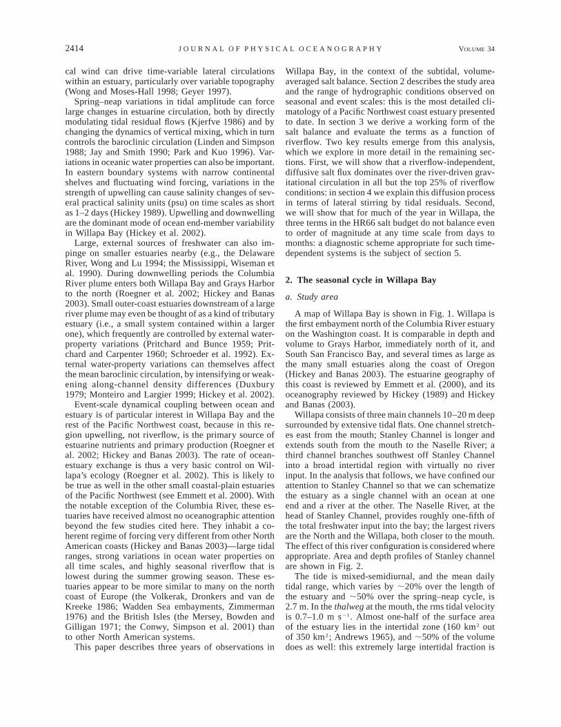
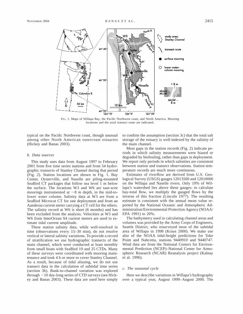
Willapa consists of three main channels 10–20 m deepsurrounded by extensive tidal flats. One channel stretch-es east from the mouth; Stanley Channel is longer andextends south from the mouth to the Naselle River; athird channel branches southwest off Stanley Channelinto a broad intertidal region with virtually no riverinput. In the analysis that follows, we have confined ourattention to Stanley Channel so that we can schematizethe estuary as a single channel with an ocean at oneend and a river at the other. The Naselle River, at thehead of Stanley Channel, provides roughly one-fifth ofthe total freshwater input into the bay; the largest riversare the North and the Willapa, both closer to the mouth.The effect of this river configuration is considered whereappropriate. Area and depth profiles of Stanley channelare shown in Fig. 2.
The tide is mixed-semidiurnal, and the mean dailytidal range, which varies by ;20% over the length ofthe estuary and ;50% over the spring–neap cycle, is2.7 m. In the thalweg at the mouth, the rms tidal velocityis 0.7–1.0 m s21. Almost one-half of the surface areaof the estuary lies in the intertidal zone (160 km2 outof 350 km2; Andrews 1965), and ;50% of the volumedoes as well: this extremely large intertidal fraction is
NOVEMBER 2004 2415B A N A S E T A L .
FIG. 1. Maps of Willapa Bay, the Pacific Northwest coast, and North America. Mooringlocations and the axial transect route are indicated.
typical on the Pacific Northwest coast, though unusualamong other North American outercoast estuaries(Hickey and Banas 2003).
b. Data sources
This study uses data from August 1997 to February2001 from five time series stations and from 54 hydro-graphic transects of Stanley Channel during that period(Fig. 2). Station locations are shown in Fig. 1. BayCenter, Oysterville, and Naselle are piling-mountedSeaBird CT packages that follow sea level 1 m belowthe surface. The locations W3 and W6 are taut-wiremoorings instrumented at ;8 m depth, in the mid-to-lower water column. Salinity data at W3 are from aSeaBird Microcat CT for one deployment and from anAanderaa current meter carrying a CT cell for the others.The salinity record at W6 is short (6 months) and hasbeen excluded from the analysis. Velocities at W3 andW6 from InterOcean S4 current meters are used to es-timate tidal current amplitude.
These station salinity data, while well-resolved intime (observations every 15–30 min), do not resolvevertical or lateral salinity variations. To provide a recordof stratification we use hydrographic transects of themain channel, which were conducted at least monthlyfrom small boats with SeaBird 19 and 25 CTDs. Manyof these surveys were coordinated with mooring main-tenance and took 4 h or more to cover Stanley Channel.As a result, because of tidal aliasing, we do not usetransect data in the calculation of subtidal time series(section 3b). Bank-to-channel variation was exploredthrough ;10 day-long series of CTD surveys (see Hick-ey and Banas 2003). These data are used here simply
to confirm the assumption (section 3c) that the total saltstorage of the estuary is well-indexed by the salinity ofthe main channel.
Most gaps in the station records (Fig. 2) indicate pe-riods in which salinity measurements were biased ordegraded by biofouling, rather than gaps in deployment.We report only periods in which salinities are consistentbetween station and transect observations. Station tem-perature records are much more continuous.
Estimates of riverflow are derived from U.S. Geo-logical Survey (USGS) gauges 12013500 and 12010000on the Willapa and Naselle rivers. Only 19% of Wil-lapa’s watershed lies above these gauges: to calculatebay-total flow, we multiply the gauged flows by theinverse of this fraction (Lincoln 1977). The resultingestimate is consistent with the annual mean value re-ported by the National Oceanic and Atmospheric Ad-ministration/Environmental Protection Agency (NOAA/EPA 1991) to 20%.
The bathymetry used in calculating channel areas andvolumes was provided by the Army Corps of Engineers,Seattle District, who resurveyed most of the subtidalarea of Willapa in 1998 (Kraus 2000). We make usealso of the NOAA tidal-height predictions for TokePoint and Nahcotta, stations 9440910 and 9440747.Wind data are from the National Centers for Environ-mental Prediction (NCEP)–National Center for Atmo-spheric Research (NCAR) Reanalysis project (Kalnayet al. 1996).
c. The seasonal cycle
Here we describe variations in Willapa’s hydrographyover a typical year, August 1999–August 2000. The
2416 VOLUME 34J O U R N A L O F P H Y S I C A L O C E A N O G R A P H Y
FIG. 2. (a) Depth of the main channel, channel width (measuredshore-to-shore), cross-sectional area, and the scale length la (upstreamvolume divided by cross-sectional area) along Stanley Channel fromthe Naselle River to the estuary mouth. (b) Data coverage of StanleyChannel, Aug 1997–Feb 2001: vertical lines indicate station timeseries; horizontal lines show main-channel CTD transects.
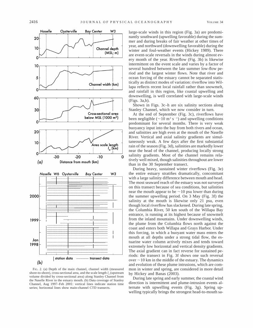
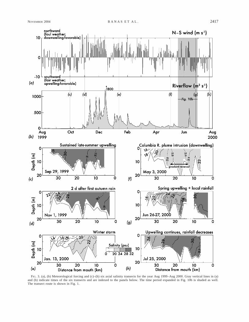
large-scale winds in this region (Fig. 3a) are predomi-nantly southward (upwelling favorable) during the sum-mer and during breaks of fair weather at other times ofyear, and northward (downwelling favorable) during thewinter and foul-weather events (Hickey 1989). Thereare event-scale reversals in the winds during almost ev-ery month of the year. Riverflow (Fig. 3b) is likewiseintermittent on the event scale and varies by a factor ofseveral hundred between the late summer low-flow pe-riod and the largest winter flows. Note that river andocean forcing of the estuary cannot be separated statis-tically as distinct modes of variation: riverflow into Wil-lapa reflects recent local rainfall rather than snowmelt,and rainfall in this region, like coastal upwelling anddownwelling, is well correlated with large-scale winds(Figs. 3a,b).
Shown in Figs. 3c–h are six salinity sections alongStanley Channel, which we now consider in turn.
At the end of September (Fig. 3c), riverflows havebeen negligible (;10 m3 s21) and upwelling conditionspredominant for several months. There is very weakbuoyancy input into the bay from both rivers and ocean,and salinities are high even at the mouth of the NaselleRiver. Vertical and axial salinity gradients are simul-taneously weak. A few days after the first substantialrain of the season (Fig. 3d), salinities are markedly lowernear the head of the channel, producing locally strongsalinity gradients. Most of the channel remains rela-tively well mixed, though salinities throughout are lowerthan in the 30 September transect.
During heavy, sustained winter riverflows (Fig. 3e)the entire estuary stratifies dramatically, concomitantwith a large salinity difference between mouth and head.The most seaward reach of the estuary was not surveyedon this transect because of sea conditions, but salinitiesnear the mouth appear to be ;10 psu lower than duringthe summer upwelling period. On 3 May (Fig. 3f) thesalinity at the mouth is likewise only 21 psu, eventhough local riverflow has slackened. During late spring,the Columbia River, 50 km south of the Willapa Bayentrance, is running at its highest because of snowmeltfrom the inland mountains. Under downwelling winds,the plume from the Columbia flows north against thecoast and enters both Willapa and Grays Harbor. Underthis forcing, in which a buoyant water mass enters themouth at all depths under a strong tidal flow, the es-tuarine water column actively mixes and tends towardextremely low horizontal and vertical density gradients.The axial gradient can in fact reverse for sustained pe-riods: the transect in Fig. 3f shows one such reversalover ;10 km in the middle of the estuary. The dynamicsand evolution of these plume intrusions, which are com-mon in winter and spring, are considered in more detailby Hickey and Banas (2003).
During late spring and early summer, the coastal winddirection is intermittent and plume-intrusion events al-ternate with upwelling events (Fig. 3g). Spring up-welling typically brings the strongest head-to-mouth sa-
NOVEMBER 2004 2417B A N A S E T A L .
FIG. 3. (a), (b) Meteorological forcing and (c)–(h) six axial salinity transects for the year Aug 1999–Aug 2000. Gray vertical lines in (a)and (b) indicate times of the six transects and are indexed to the panels below. The time period expanded in Fig. 10b is shaded as well.The transect route is shown in Fig. 1.
2418 VOLUME 34J O U R N A L O F P H Y S I C A L O C E A N O G R A P H Y
linity differences of the year. Finally, as riverflow slack-ens over the course of the summer (Fig. 3h), salinity atthe head increases, and vertical and horizontal gradientsweaken. The bay thus gradually returns to the nearly-well-mixed conditions shown in Fig. 3c. Event-scalewind reversals interrupt this trend (Fig. 3a), though notas dramatically as during early summer.
As these six snapshots suggest, over the course of ayear Willapa Bay cycles or weaves over an enormousrange of the possible hydrographic states of a partiallymixed estuary. Because ocean and river forcing are bothso variable—and because the impact of event-scaleocean variability is not confined to the mouth, but ratherpenetrates through most of the volume of the bay—nomonotonic relationship exists between either ocean sa-linity or riverflow and estuarine salinity gradients. Nev-ertheless, we can estimate the relative roles of time de-pendence, riverflow, gravitational circulation, and othersalt-loading mechanisms using a simplified form of thevolume-integrated salt balance. This calculation is thesubject of the next section.
3. The salt balance
a. Theory
We will begin by deriving our working form of thesalt balance; in section 3b we describe our methods forcalculating the terms in this balance from data, and insection 3c and 3d we use these tools to describe thedynamics of Willapa Bay across forcing conditions.
We start with a general budget equation for salt, inwhich we have averaged over a cross section of theestuary (denoted by an overbar), averaged as well overthe tidal cycle (angle brackets), and finally integratedin the axial (x) direction from far upstream where saltflux is zero (x 5 2`) to x:
x]^as& dx 1 ^aus& 5 0. (3.1)E]t
2`
Here t is time, s is salinity, u is axial velocity, and a iscross-sectional area. The first term describes subtidalchanges in total salt storage upstream of x on subtidaltime scales, and the second denotes total salt fluxthrough the cross section at x. The integral in the firstterm can be written more simply as V , where V is meansvolume upstream of x and the mean salinity over thatsvolume. We also can define an area length scale la [V^a&21 so that (3.1) becomes
]s 1l 1 ^aus& 5 0. (3.2)a ]t ^a&
Values of la along Stanley Channel are given in Fig. 2.Note that we have assumed a term on the left-hand sideinvolving ]V/]t, and thus wind-driven sea level setupand setdown, to be small. In other estuaries this termmay in fact be more important than the ] /]t term, butsHickey et al. (2002) found that the large-scale winds
affect circulation in Willapa primarily through upwell-ing- and downwelling-related salinity changes and notbarotropic volume changes.
All the mechanisms that move salt up- and down-stream are contained within the total flux term ^a &. Auscommon approach, beginning with HR65, has been todecompose this flux into three terms as follows:
]^s&^aus& 5 ^a& ^u&^s& 1 ^u9s9& 2 K . (3.3)1 2]x
Here u9 and s9 are defined as spatial fluctuations aroundand such that [ [ 0, and K is a horizontalu s u9 s9
diffusivity. The first term on the right-hand side rep-resents seaward advection of salt by the mean flow: uis related to riverflow Q by
^Q& 5 ^au&, (3.4)
where again we have ignored sea level setup- and set-down-driven volume changes (an assumption that maynot be valid if the salt balance is to be evaluated not inlong averages, as we do below, but on the event scale).We will refer to ^ &^ & as the ‘‘river’’ or ‘‘river-flushing’’u sterm. The second term in (3.3) describes correlationsbetween the mean vertical structures of velocity andsalinity: in the HR65 theory this correlation describesa steady vertical exchange flow or gravitational circu-lation. Last, the third, or diffusion, term, parameterizesall remaining correlations between a, u, and s: Stokesdrift (tidal correlations between a and u), ‘‘tidal trap-ping’’ in side channels or on banks (tidal correlationsbetween u and s), stirring by tidal residuals (lateral cor-relations between ^u& and ^s&), and several other terms.For more detailed discussion of these terms, see Fischer(1976); for full empirical salt-flux decompositions inindividual estuaries, see Hughes and Rattray (1980),Winterwerp (1983), Lewis and Lewis (1983), and Dron-kers and van de Kreeke (1986).
In the steady case (] /]t 5 0), (3.2), (3.3), and (3.4)sbecome the classical HR66 salt balance:
Q ]ss 5 2u9s9 1 K . (3.5)
a ]x
We have dropped the angle brackets for brevity. In thiscase, total upstream salt flux (the right-hand side) exactlybalances river-flushing, and is partitioned between a steadygravitational circulation and an undifferentiated diffusionprocess. A classification parameter y, the diffusive fractionof upstream salt flux, can then be defined as
]sK
]xy [ . (3.6)
]su9s9 1 K
]x
When y 5 0 river-flushing balances gravitational cir-culation, and when y 5 1 river-flushing balances dif-fusion. A more general scheme that diagnoses the full
NOVEMBER 2004 2419B A N A S E T A L .
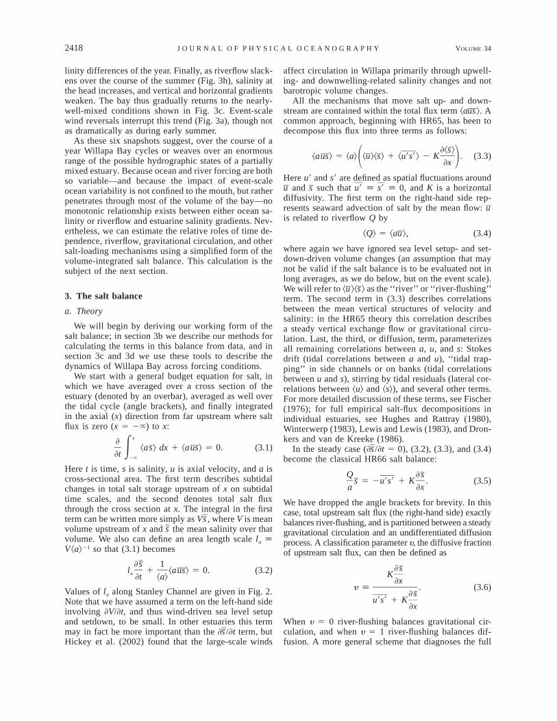
FIG. 4. Surface-to-bottom salinity difference at Bay Center andNaselle from transect data, shown as a function of riverflow. Dataare instantaneous and therefore tidally aliased.
unsteady salt balance as y diagnoses the steady HR66balance is the subject of section 5.
In an estuary where stratification and shear vary sig-nificantly over the tidal cycle (Jay and Smith 1988; Sta-cey et al. 2001) or vary laterally because of Coriolis ortopography (Li and O’Donnell 1997), it may be mis-leading to equate the gravitational circulation with themean quantity . Since in the present study we lacku9s9the data to decompose ^a & with enough detail to re-ussolve these effects, we will use a formulation even sim-pler than the HR65 decomposition (3.3):
]^s&^aus& 5 ^a& ^u&^s& 1 K . (3.7)tot1 2]x
Here Ktot is a total effective diffusivity, which param-eterizes all upstream salt-flux mechanisms, including thegravitational circulation. Combining (3.7) with (3.2) and(3.4) yields the general unsteady salt balance
]s Q ]sl 1 s 5 K , (3.8)a tot]t a ]x
where again we have dropped the angle brackets. We candiagnose the unsteadiness of the salt balance by com-paring Ktot with an equilibrium value , defined byeqK tot
Q ]seqs 5 K . (3.9)tota ]x
When Ktot , , river-flushing exceeds upstream salteqK tot
flux and the estuary loses salt; when Ktot . , theeqK tot
estuary gains salt. We will evaluate Ktot and foreqK tot
Willapa in section 3c.This total-diffusivity approach, with and without the
assumption of a steady state, has been used in a numberof studies (e.g, Uncles and Stephens 1990; Monismithet al. 2002; Lewis and Uncles 2003). It is convenientwhere data are sparse, but it has the drawback of leavingthe dynamics of upstream salt flux ambiguous. In section3d, we will describe an empirical decomposition of Ktot
that to some extent allows us to recover the dynamicalinformation in the HR66 formulation.
b. Calculation methods
Before continuing with the Ktot calculation, in thissection we discuss the methods by which the spatiallyintegrated quantities , ] /]t, and ] /]x are estimateds s sfrom our point measurements.
For simplicity we let station salinities represent swithout adjustment: i.e., we ignore vertical and lateralsalinity variations. (The error associated with this andour other approximations is discussed below.) We cal-culate ] /]x not as a difference between stations, but assa point measurement at each station, taking advantageof the fact that over a tidal cycle each station samplesa full tidal excursion of the channel. Dividing the dif-ference between end-of-flood and end-of-ebb salinity bythe tidal excursion gives one value of ] /]x for eachs
tidal cycle, and low-pass-filtering this discrete seriesgives a continuous subtidal time series. This method,unlike differencing between stations, gives a truly localmeasure of ] /]x and is unaffected by gaps in coveragesat other stations. Last, to evaluate ] /]t we calculatestotal upstream salt storage V as a linear combinationsof landward station salinities; for example, at Bay Cen-ter,
](V s)Bay Ctr]t
]9 35 (0.25s 1 0.20s 1 0.06s ) 3 10 m .Bay Ctr Oyst Naselle]t(3.10)
The coefficients are calculated from total volume belowMSL between each pair of stations.
We estimate from axial and lateral transect data thatat Bay Center, the total uncertainty in associated withsunresolved salinity variations in all three dimensions isonly ;10%. This level is set by the maximum discrep-ancy between measured (surface) salinity and vertical-mean salinity taking into account stratification (Fig. 4).Errors from lateral salinity variations are less than 10%:differential tidal advection has been seen to create bank-to-channel salinity variations near Bay Center of severalpractical salinity units (Hickey and Banas 2003) butthese gradients are only strong over very shallow banks,where their volume-integrated effect is smallest. Stationspacing in the axial direction is comparable to the tidalexcursion and accordingly appears sufficient to resolvesubtidal axial salinity variations throughout the bay.
A potentially much larger—and harder to quantify—source of uncertainty is the proximity of W3 and Oys-terville to the subestuaries outside Stanley Channel. Inparticular, 80% of riverflow into the bay enters between

2420 VOLUME 34J O U R N A L O F P H Y S I C A L O C E A N O G R A P H Y
FIG. 5. (a), (b) Regression between the left-hand side of (3.8)—the time-change and river-flushing terms—and axial salinity gradient atBay Center for two riverflow bins. The slope of the regression is the effective diffusivity Ktot. (c) The diffusivity Ktot calculated as in (a)and (b) for all riverflow bins, along with the equilibrium value , calculated by analogous regressions between the river term alone andeqK tot
] /]x [(3.9)]. Shaded areas give 95% confidence limits. The dashed horizontal line shows the value of the low-flow diffusivity K as definedsin section 3d. A histogram of riverflow values over the three-year study period is also shown.
Bay Center and W3, but the lateral distribution of thisfreshwater around W3 and the mouth of the bay is un-clear: sea conditions make Willapa’s entrance shoalsimpossible to survey from a small boat. As a result, inthe analysis that follows, we evaluate the salt balanceat Bay Center, where the geometry is simplest and ourdata coverage best, in the most detail.
c. Total effective diffusivity
We now have estimates of every quantity in (3.8)except for Ktot and can in principle solve for Ktot as acontinuous subtidal time series. In practice, it is morestatistically robust to calculate Ktot in an ensemble av-erage, as the mean slope between the left-hand side of(3.8) and ] /]x for some set of measurements. We willsstart by binning observations by bay-total riverflow, asa proxy for meteorological forcing in general.
Results of the Ktot calculation for Bay Center areshown in Fig. 5. Individual data points for two riverflowbins are shown in Figs. 5a and 5b, and ensemble av-erages for all bins are shown in Fig. 5c along with 95%confidence limits. These confidence limits are generally
larger than the observational uncertainties estimatedabove: they thus appear to represent not error but real,ocean-forced variability within each riverflow bin. Datahave been Butterworth-filtered with a cutoff frequencyof (10 days)21, to average over the mean propagationtime for ocean signals from the mouth to the head atNaselle (see section 4c). Shorter and longer filter periodschange the magnitude of the variance within each riv-erflow bin but have a statistically insignificant effect onKtot itself. This is one validation of the appropriatenessof the total-diffusivity model.
Ktot increases with riverflow Q from 240 m2 s21 atvery low flows to 840 m2 s21 at high flows: a changeof a factor of 3.5. In comparison, the equilibrium value
increases by more than a factor of 20 over the sameeqK tot
riverflow range, from 50 to 1100 m2 s21. Willapa is thusfar from equilibrium over nearly all flow conditions.For Q , 300 m3 s21 (85% of observations), upstreamsalt flux exceeds river-flushing (Ktot . ) and the es-eqK tot
tuary gains salt. This is true on average: it is not nec-essarily true during individual, transient, ocean-forcedevents like Columbia plume intrusions. During highwinter flows above 300 m3 s21, on average the river-

NOVEMBER 2004 2421B A N A S E T A L .
flushing term dominates (Ktot , ) and the estuaryeqK tot
loses salt. Integrated over a full seasonal cycle, the saltbudget does appear to balance: the mean Ktot and eqK tot
for the 1-yr period shown in Fig. 3 agree, perhaps co-incidentally, within 2% (not shown).
d. Decomposition of upstream salt flux
In low-flow conditions, the difference between Ktot
and is actually many times larger than itselfeq eqK Ktot tot
(Fig. 5). This is only possible if the river term in (3.8)is negligible and the dominant balance is between theKtot term and the time-change term, i.e., an unsteadydiffusion process independent of riverflow. StanleyChannel thus appears more like a lagoon or riverlesstidal embayment than like a true estuary during the sum-mer low-flow period.
These simplified low-flow-period dynamics suggestan empirical division of up-estuary salt flux into river-driven and river-independent parts, analogous to theHR66 partitioning between river-driven gravitationalcirculation and ‘‘true’’ diffusion. We can write this asKtot [ Kgc 1 K, where K is defined as the ‘‘baseline’’or low-riverflow limit of Ktot (the dashed line in Fig. 5).The salt balance (3.8) then becomes
]s Q ]s ]sl 1 s 5 K 1 K . (3.11)a gc]t a ]x ]x
The Kgc term is analogous to, but more general than,the in the HR66 formulation (3.5). More precisely,u9s9Kgc represents both the mean gravitational circulation ata given riverflow level and all nonlinear coupling be-tween this gravitational circulation and diffusive ex-change. K, the ‘‘true’’ diffusivity, represents a combi-nation of tidal exchange (lateral stirring, trapping,Stokes drift), local-wind-driven processes, and modu-lations of the mean gravitational circulation by oceandensity fluctuations (‘‘baroclinic coupling’’; Hickey etal. 2002).
The purpose of this decomposition is to isolate K sothat its dependence on forcing can be examined, and adynamical explanation obtained for the high, unequili-brated rate at which Willapa loads seawater during low-flow conditions. In section 4 we will demonstrate thatK is primarily a tide-driven, rather than baroclinic, pro-cess, and present a scaling that explains its variationover the length of Stanley Channel.
4. Tidal diffusion in low-flow conditions
a. Calculation of K
We begin by calculating K for all stations. Instead ofrepeating the full determination of Ktot(Q) at every sta-tion besides Bay Center—data gaps and the geometriccomplexity discussed in section 3b make this difficult—we will use a simpler method. By definition, as Q →0, (3.8) approaches the diffusive limit
]s ]sl 5 K . (4.1)a ]t ]x
Thus K can be calculated as the slope between the time-change term and ] /]x in the average over all low-flowsconditions. ‘‘Low flows’’ are those for which the ne-glected river term is smaller than the standard deviationof the time-change term around its correlation with ] /s]x, and thus by definition well-contained within 95%confidence limits. To err on the side of an over-strictdefinition of low flows, we compute this threshhold us-ing bay-total riverflow for Q. At Naselle, salinity var-iance in summer is so small that even if we take Q tobe Naselle flow alone, our low-flow definition excludesthe entire record; results are given for Naselle riverflows,2 m3 s21.
Results are shown in Fig. 6 for all four stations. Asin section 3, the data have been filtered with a cutofffrequency of (10 days)21. Mean values of K decreasefrom 710 m2 s21 at W3 to 20 m2 s21 at Naselle. Theestimate at Naselle is not different from zero at the 95%confidence level, but it is a stable result, $20 m2 s21
regardless of the choice of filter timescale or riverflowthreshold. The estimate at Bay Center calculated by thismethod agrees within confidence limits with the baselineKtot shown in Fig. 5.
A number of factors presumably contribute to thescatter of individual events around the long-term mean:baroclinic ocean-estuary coupling, the small but non-zero river-driven salt fluxes permitted under our defi-nition of ‘‘low flows,’’ spring–neap variations in tidalstirring (section 4c), lateral circulations driven by localwind, and non-Fickian tidal dispersion mechanisms (i.e.,tidal salt fluxes not proportional to ] /]x; Ridderinkhofsand Zimmerman 1992; McCarthy 1993). For many in-dividual events, the net salt flux explained by the con-stant-diffusivity regression is smaller than the salt fluxit does not explain.
Nevertheless, a constant diffusivity explains one-halfor more of the variance in 10-day and longer-scale saltfluxes everywhere except the river mouth itself (at W3and Bay Center, the regressions in Fig. 6 have r2 5 0.7;at Oysterville, r2 5 0.5). In the sections that follow weexamine the physical meaning of this very simple salt-flux parameterization.
b. Signal penetration and propagation speed
A constant K is only a satisfactory parameterizationof up-estuary salt flux in low-flow conditions if it re-produces both the propagation rate and penetration dis-tance observed for ocean signals. To derive predictionsof these parameters from the axial profile of K calculatedabove, we numerically integrated the differential formof (4.1)
]s ] ]sa 5 aK , (4.2)1 2]t ]x ]x

2422 VOLUME 34J O U R N A L O F P H Y S I C A L O C E A N O G R A P H Y
FIG. 6. (a) Time-change term vs axial salinity gradient at eachStanley Channel station, in low-flow conditions. The slope of theregressions (solid lines) is the diffusivity K. (b) Diffusivities from(a) shown as an along-channel profile. Dashed lines give 95% con-fidence limits on the slope.
FIG. 7. (a) Lag times in days relative to W3 and (b) relative am-plitude of the part of the signal correlated with W3, for detrendedsalinity data from Jul–Sep 1999 (dots) and a numerical solution to(4.2) for the same time period (lines).
using a simple forward-in-time, centered-in-spacescheme, with data from W3 supplying the seawardboundary condition. Numerical results cannot be com-pared point-by-point with station salinities, both be-cause of the neglected exchanges between StanleyChannel and the other subestuaries, and because even;10% biases in ] /]t (see section 3b) quickly becomesO(1) errors in the time-integral. Instead, to isolate up-
stream-propagating signals, we calculate lag times ofmaximum correlation with W3 and amplitude of thecorrelated part of the signal (i.e., slope between salinityat each station and at W3). Results are shown in Fig. 7for the low-flow period July–September 1999, and thereach of Stanley Channel from the mouth to Oysterville.Naselle and the small volume at the head of the channel,where signal penetration is weak and K is poorly con-strained, are omitted.
The numerical solution follows the empirical patternwith reasonable accuracy, and reproduces, qualitatively,the rapid propagation of signals to Bay Center and theabrupt slowdown between Bay Center and Oysterville.Note that the propagation rate and penetration distanceof ocean signals depend as much on the frequency ofthe boundary forcing as on the internal dynamics of theestuary. If single-frequency forcing is used in place ofdata from W3, (4.2) becomes the classical oscillatoryboundary layer problem (Batchelor 1967, p. 353ff ), and
NOVEMBER 2004 2423B A N A S E T A L .
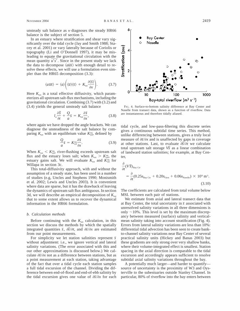
FIG. 8. Diffusivities from Fig. 6 compared with the product of tidalvelocity and channel width. The predicted scaling (4.3) is shown forthree values of cK.
the numerical solution reproduces the expected rela-tionships among propagation rate, penetration distance,and forcing frequency.
c. Dynamics of ‘‘diffusion’’
What physical meaning can be given to the magnitudeof K, and to its 30-fold decrease over the length ofStanley Channel (Fig. 6)? We wrote above that K rep-resents a combination of tide-, wind-, and ocean-den-sity-driven mechanisms. Hickey et al. (2002) find thatthe distribution of residual currents in Willapa suggeststide- and density-driven circulations more than local-wind-driven circulations: we cannot quantify the localwind contribution more than this with available data,but we can guess that it does not set the scale of K.This leaves tidal and baroclinic mechanisms and thecoupling between them.
Zimmerman (1986) offers two models to explain thelarge (100–1000 m2 s21) diffusivities commonly ob-served in tidal waters. The first consists of a cascade ofturbulent processes, in which lateral shears amplify dis-persion by vertical shears, which in turn amplify dis-persion by small-scale turbulence proper. The secondrelies on lateral shears alone. He proposes dispersionby ‘‘Lagrangian chaos,’’ in which the tidally averagedflow field is deterministic and steady but spatially com-plex—randomized by bathymetry rather than by tur-bulence—so that Lagrangian trajectories through thatflow field are strongly divergent. Complex tidal-residualflow fields are often observed (Kuo et al. 1990; Li andO’Donnell 1997; Blanton and Andrade 2001) and thedivergence of trajectories in a such a field is clear fromsimulation (Ridderinkhof and Zimmerman 1992). Theopen question is how commonly this type of density-independent tidal dispersion dominates over baroclinicmechanisms, or interactions between tidal and baro-clinic mechanisms (Smith 1996; Valle-Levinson andO’Donnell 1996), in estuaries with measurable strati-fication.
In the remainder of this section we will verify theconsistency of the simplest possibility for Willapa’s low-flow period dynamics: that the bathymetric tidal-resid-ual field alone sets the scale of K in the long-term av-erage, even if the dynamics of individual events arepartly baroclinic or wind-driven. We hypothesize thenthat K scales with the amplitude and width of the largestresidual eddies (MacCready 1999). Since in Willapa thetidal excursion is greater than the width of the estuary,this model implies
K ø c U b,K T (4.3)
where cK is a constant of proportionality O(1) or smaller,UT is the rms tidal velocity, and b is the channel width.The empirical values of K calculated in section 4a areshown as a function of UTb in Fig. 8. We calculate bas cross-sectional area divided by mean depth belowmean sea level. Among the four stations cK varies be-
tween 0.03 and 0.09: if residual velocities are 10%–20% of the rms tidal amplitude as Zimmerman (1986)suggests is generally true and residual eddies are rough-ly one-half of the width of the estuary, we would expectcK 5 0.05–0.1. The conceptual model behind (4.3) isthus consistent. Since UT varies only fractionally overthe length of Stanley Channel and b varies by a factorof 9, this correlation primarily tests the dependence ofK on b.
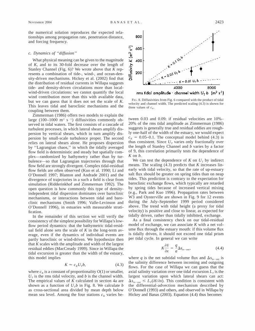
We can test the dependence of K on UT by indirectmeans. The scaling (4.3) predicts that K increases lin-early with tidal velocity, so that the rate of up-estuarysalt flux should be greater on spring tides than on neaptides. This prediction is contrary to the expectation forbaroclinic exchange flows, which typically are retardedby spring tides because of increased vertical mixing(e.g., Park and Kuo 1996). Propagation rates betweenW3 and Oysterville are shown in Fig. 9 for 12 eventsduring the July–September 1999 period consideredabove. The trend with tidal height (a proxy for tidalvelocity) is positive and close to linear, as expected fortidally driven, rather than tidally inhibited, exchange.
As a final consistency check on our tidal-residualmodel of exchange, we can associate K with a net vol-ume flux through the estuary mouth: if this volume fluxis tidally driven, it should not exceed one tidal prismper tidal cycle. In general we can write
]s qK 5 Ds , (4.4)in2out]x a
where q is the net subtidal volume flux and Dsin2out isthe salinity difference between incoming and outgoingflows. For the case of Willapa we can guess that theaxial salinity variation over one tidal excursion LT is thelargest variation upon which lateral shears can act:Dsin2out # LT(] /]x). This condition is consistent withsthe differential-advection mechanism described byO’Donnell (1993) and others, and observed in Willapa byHickey and Banas (2003). Equation (4.4) thus becomes
2424 VOLUME 34J O U R N A L O F P H Y S I C A L O C E A N O G R A P H Y
FIG. 9. (a) Detrended subtidal salinity at W3 and Oysterville, Jul–Sep 1999. (b) Signal propagation rate, inferred from the lagged cor-relation between W3 and Oysterville for individual maxima and min-ima in the record shown in (a) regressed to tidal amplitude.
aKq $ . (4.5)
LT
The right-hand side is roughly 3000 m3 s21 at W3,whereas Willapa’s total tidal volume flux is roughly10 000 m3 s21 (NOAA/EPA 1991). Willapa’s tidal ex-change ratio—the fraction of the tidal prism replacedby new water on the following tide—thus is $0.3, con-sistent with the range of typical values reported by Dyer(1973). Note that as a and K decrease landward, so maythe tidal exchange ratio.
5. Discussion and conclusions
a. Tide-driven exchange
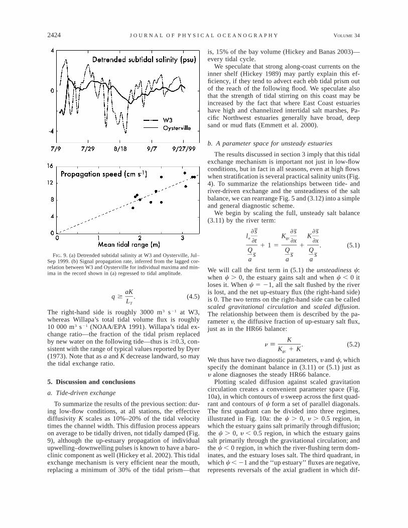
To summarize the results of the previous section: dur-ing low-flow conditions, at all stations, the effectivediffusivity K scales as 10%–20% of the tidal velocitytimes the channel width. This diffusion process appearson average to be tidally driven, not tidally damped (Fig.9), although the up-estuary propagation of individualupwelling–downwelling pulses is known to have a baro-clinic component as well (Hickey et al. 2002). This tidalexchange mechanism is very efficient near the mouth,replacing a minimum of 30% of the tidal prism—that
is, 15% of the bay volume (Hickey and Banas 2003)—every tidal cycle.
We speculate that strong along-coast currents on theinner shelf (Hickey 1989) may partly explain this ef-ficiency, if they tend to advect each ebb tidal prism outof the reach of the following flood. We speculate alsothat the strength of tidal stirring on this coast may beincreased by the fact that where East Coast estuarieshave high and channelized intertidal salt marshes, Pa-cific Northwest estuaries generally have broad, deepsand or mud flats (Emmett et al. 2000).
b. A parameter space for unsteady estuaries
The results discussed in section 3 imply that this tidalexchange mechanism is important not just in low-flowconditions, but in fact in all seasons, even at high flowswhen stratification is several practical salinity units (Fig.4). To summarize the relationships between tide- andriver-driven exchange and the unsteadiness of the saltbalance, we can rearrange Fig. 5 and (3.12) into a simpleand general diagnostic scheme.
We begin by scaling the full, unsteady salt balance(3.11) by the river term:
]s ]s ]sl K Ka gc]t ]x ]x
1 1 5 1 . (5.1)Q Q Q
s s sa a a
We will call the first term in (5.1) the unsteadiness c:when c . 0, the estuary gains salt and when c , 0 itloses it. When c 5 21, all the salt flushed by the riveris lost, and the net up-estuary flux (the right-hand side)is 0. The two terms on the right-hand side can be calledscaled gravitational circulation and scaled diffusion.The relationship between them is described by the pa-rameter y, the diffusive fraction of up-estuary salt flux,just as in the HR66 balance:
Kn [ . (5.2)
K 1 Kgc
We thus have two diagnostic parameters, y and c, whichspecify the dominant balance in (3.11) or (5.1) just asy alone diagnoses the steady HR66 balance.
Plotting scaled diffusion against scaled gravitationcirculation creates a convenient parameter space (Fig.10a), in which contours of y sweep across the first quad-rant and contours of c form a set of parallel diagonals.The first quadrant can be divided into three regimes,illustrated in Fig. 10a: the c . 0, y . 0.5 region, inwhich the estuary gains salt primarily through diffusion;the c . 0, y , 0.5 region, in which the estuary gainssalt primarily through the gravitational circulation; andthe c , 0 region, in which the river-flushing term dom-inates, and the estuary loses salt. The third quadrant, inwhich c , 21 and the ‘‘up estuary’’ fluxes are negative,represents reversals of the axial gradient in which dif-
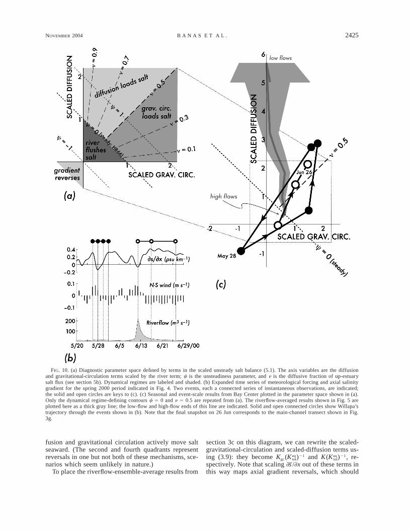
NOVEMBER 2004 2425B A N A S E T A L .
FIG. 10. (a) Diagnostic parameter space defined by terms in the scaled unsteady salt balance (5.1). The axis variables are the diffusionand gravitational-circulation terms scaled by the river term; c is the unsteadiness parameter, and n is the diffusive fraction of up-estuarysalt flux (see section 5b). Dynamical regimes are labeled and shaded. (b) Expanded time series of meteorological forcing and axial salinitygradient for the spring 2000 period indicated in Fig. 4. Two events, each a connected series of instantaneous observations, are indicated;the solid and open circles are keys to (c). (c) Seasonal and event-scale results from Bay Center plotted in the parameter space shown in (a).Only the dynamical regime-defining contours c 5 0 and n 5 0.5 are repeated from (a). The riverflow-averaged results shown in Fig. 5 areplotted here as a thick gray line; the low-flow and high-flow ends of this line are indicated. Solid and open connected circles show Willapa’strajectory through the events shown in (b). Note that the final snapshot on 26 Jun corresponds to the main-channel transect shown in Fig.3g.
fusion and gravitational circulation actively move saltseaward. (The second and fourth quadrants representreversals in one but not both of these mechanisms, sce-narios which seem unlikely in nature.)
To place the riverflow-ensemble-average results from
section 3c on this diagram, we can rewrite the scaled-gravitational-circulation and scaled-diffusion terms us-ing (3.9): they become Kgc( )21 and K( )21, re-eq eqK Ktot tot
spectively. Note that scaling ] /]x out of these terms insthis way maps axial gradient reversals, which should
2426 VOLUME 34J O U R N A L O F P H Y S I C A L O C E A N O G R A P H Y
appear in the third quadrant, onto the first. Results forBay Center are shown in Fig. 10c: these are simply amore succinct rearrangement of the results shown in Fig.5. At low flows, the estuary is far into the ‘‘diffusionloads salt’’ regime: c k 1 and y is close to 1. At highflows, the estuary enters the ‘‘river flushes salt’’ regime.
We can place individual events in this parameterspace—very tentatively, given the limitations of the da-taset—for comparison with the riverflow-ensemble-av-erage results. Time series of wind, riverflow, and ] /]xsfrom spring 2000 are shown in Fig. 10b. Two eventsare indicated. In the first (solid circles), a short periodof northward (downwelling favorable) winds forces anaxial gradient reversal, likely an intrusion of the Co-lumbia plume. In the second (open circles), another pe-riod of northward wind accompanies a strong peak inlocal riverflow. Subtidal snapshots of conditions at BayCenter during these events, from the initial responsethrough the relaxation back to upwelling conditions, areshown in Fig. 10c. The gravitational term has been cal-culated, for lack of a better option, as the differencebetween the other terms in (5.1), so that points in theparameter space are determined by c and the verticalcoordinate. The diffusion term has been calculated usingthe long-term mean K; the scatter in Fig. 6 suggests thatthe errors here may well be O(1), and so we will interpretthese results only qualitatively.
The bay’s trajectory during the second, river-forcedevent follows the riverflow-averaged pattern: river-flushing dominates during the flow peak itself, but theestuary returns to diffusive salt loading, typical low-flow-period dynamics, over a few weeks. During thefirst event, the estuary cycles from diffusive salt-loadingto strong salt flushing and back over only 8 days. Notethat during the gradient reversal the rate of salt flushingis several times larger than the river term (c ø 22.5on 28 May; Fig. 10c). These trajectories thus illustratenot only Willapa’s changeability on the event scale, butalso the power of oceanic water-property variations toforce transient fluxes through an estuary several timesstronger than the steady, river-driven fluxes usually em-phasized in estuarine classification.
c. Generalizing to other unsteady systems
The extreme unsteadiness of the salt balance in Wil-lapa—imbalances not just on the same scale as the river-driven fluxes, but many times larger—appear to resultfrom the combination of highly variable ocean forcingwith dispersion mechanisms strong enough to propagatethese forcing fluctuations far upstream on their timescale of variation. Even in the absence of strong oceanvariability, however, variations in riverflow may stilldrive O(1) imbalances in the salt budget. Simpson et al.(2001) found a seasonal pattern very similar to Willapa’sin the Conwy in Wales, where tidal upstream salt fluxgreatly exceeds downstream river-driven flux for all ex-cept occasional high-riverflow events.
A common formalism (e.g., HR65; Kranenburg 1986)invites us to think of the estuarine salt budget as thesum of a steady balance like (3.5) and transient pro-cesses, and then to define an averaging timescale, the‘‘adjustment time,’’ above which the transients are neg-ligible. (HR65 implicitly takes the tidal period as theadjustment time.) This formalism is not germane to anestuary as strongly forced as Willapa or the Conwy,where the salt balance is only close to steady in averagesso long (1 yr or perhaps longer; section 3c) that theydo not allow us to distinguish one forcing regime fromanother. Accordingly, in section 5b we have proposeda formalism in which the unsteadiness of the salt balanceenters as part of the basis for estuarine description andclassification, rather than entering only as noise.
Acknowledgments. This work was supported bygrants NA76 RG0119 Project R/ES-9, NA76 RG0119AM08 Project R/ES-33, NA16 RG1044 Project R/ES-42, NA76 RG0485 Project R/R-1, and NA96 OP0238Project R/R-1 from the National Oceanic and Atmo-spheric Administration to Washington Sea Grant Pro-gram, University of Washington, and by Grant CR824472-01-0 from the Environmental Protection Agen-cy. NSB was also supported by a National Defense Sci-ence and Engineering Graduate fellowship. Bill Fred-ericks, Jim Johnson, and Sue Geier at the University ofWashington, and Eric Siegel, Kara Nakata, Julia Bos,and Casey Clishe at the Washington Department ofEcology were responsible for data collection and initialprocessing. Many thanks are given to Brett Dumbauldand the Washington Department of Fish and Wildlifefor their generous logistical support. Conversations withStephen Monismith were very helpful.
REFERENCES
Andrews, R. S., 1965: Modern sediments of Willapa Bay, Washing-ton: A coastal plain estuary. University of Washington Depart-ment of Oceanography Tech. Rep. 118, 48 pp.
Batchelor, G. K., 1967: An Introduction to Fluid Dynamics. Cam-bridge University Press, 615 pp.
Blanton, J. O., and F. A. Andrade, 2001: Distortion of tidal currentsand the lateral transfer of salt in a shallow coastal plain estuary(O Estuario do Mira, Portugal). Estuaries, 24, 467–480.
Bowden, K. F., and R. M. Gilligan, 1971: Characterisation of featuresof estuarine circulation as represented in the Mersey Estuary.Limnol. Oceanogr., 16, 490–502.
Dronkers, J., and J. van de Kreeke, 1986: Experimental determinationof salt intrusion mechanisms in the Volkerak estuary. Neth. J.Sea Res., 20, 1–19.
Duxbury, A. C., 1979: Upwelling and estuary flushing. Limnol.Oceanogr., 24, 627–633.
Dyer, K. R., 1973: Estuaries: A Physical Introduction. John Wileyand Sons, 140 pp.
Emmett, R., and Coauthors, 2000: Geographic signatures of NorthAmerican West Coast estuaries. Estuaries, 23, 765–792.
Fischer, H. B., 1976: Mixing and dispersion in estuaries. Annu. Rev.Fluid Mech., 8, 107–133.
Geyer, W. R., 1997: Influence of wind on dynamics and flushing ofshallow estuaries. Estuarine Coastal Shelf Sci., 44, 713–722.
Gibson, J. R., and R. G. Najjar, 2000: The response of Chesapeake
NOVEMBER 2004 2427B A N A S E T A L .
Bay salinity to climate-induced changes in streamflow. Limnol.Oceanogr., 45, 1764–1772.
Hansen, D. V., and M. Rattray Jr., 1965: Gravitational circulation instraits and estuaries. J. Mar. Res., 23, 104–122.
——, and ——, 1966: New dimensions in estuary classification. Lim-nol. Oceanogr., 11, 319–326.
Hickey, B. M., 1989: Patterns and processes of circulation over theshelf and slope. Coastal Oceanography of Washington andOregon, B. M. Hickey and M. R. Landry, Eds., Elsevier, 41–115.
——, and N. S. Banas, 2003: Oceanography of the U.S. Pacific North-west coastal ocean and estuaries with application to coastal ecol-ogy. Estuaries, 26, 1010–1031.
——, X. Zhang, and N. Banas, 2002: Coupling between the CaliforniaCurrent System and a coastal plain estuary in low riverflowconditions. J. Geophys. Res., 107, 3166, 10.1029/1999JC000160.
Hughes, R. P., and M. Rattray, 1980: Salt flux and mixing in the Co-lumbia River Estuary. Estuarine Coastal Mar. Sci., 10, 479–494.
Jay, D. A., and J. D. Smith, 1988: Residual circulation in and clas-sification of shallow, stratified estuaries. Physical Processes inEstuaries, J. Dronkers and W. van Leussen, Eds., Springer-Ver-lag, 21–41.
——, and ——, 1990: Residual circulation in shallow, stratified es-tuaries. Part II: Weakly-stratified and partially-mixed systems.J. Geophys. Res., 95, 733–748.
Kalnay, E., and Coauthors, 1996: The NCEP/NCAR 40-Year Re-analysis Project. Bull. Amer. Meteor. Soc., 77, 437–471.
Kjerfve, B., 1986: Circulation and salt flux in a well mixed estuary.Physics of Shallow Estuaries and Bays, J. van de Kreeke, Ed.,Springer-Verlag, 22–29.
Kranenburg, C., 1986: A timescale for long-term salt intrusion inwell-mixed estuaries. J. Phys. Oceanogr., 16, 1329–1331.
Kraus, N. C., Ed., 2000: Study of Navigation Channel Feasibility,Willapa Bay, Washington. U.S. Army Engineer District FinalReport, 440 pp.
Kuo, A. Y., J. M. Hamrick, and G. M. Sisson, 1990: Persistence ofresidual currents in the James River estuary and its implicationto mass transport. Residual Currents and Long-Term Transport,R. T. Cheng, Ed., Springer-Verlag, 389–401.
Lewis, R. E., and J. O. Lewis, 1983: The principal factors contributingto the flux of salt in a narrow, partially stratified estuary. Es-tuarine Coastal Shelf Sci., 33, 599–626.
——, and R. J. Uncles, 2003: Factors affecting longitudinal dispersionin estuaries of different scale. Ocean Dyn., 53, 197–207.
Li, C., and J. O’Donnell, 1997: Tidally induced residual circulationin shallow estuaries with lateral depth variation. J. Geophys.Res., 102, 27 915–27 929.
Lincoln, J. H., 1977: Derivation of freshwater inflow into PugetSound. University of Washington Department of OceanographySpecial Rep. 72, 20 pp.
Linden, P. F., and J. E. Simpson, 1988: Modulated mixing and frontogenesisin shallow seas and estuaries. Cont. Shelf Res., 8, 1107–1127.
MacCready, P., 1999: Estuarine adjustment to changes in river flowand tidal mixing. J. Phys. Oceanogr., 29, 708–726.
McCarthy, R. K., 1993: Residual currents in tidally dominated, well-mixed estuaries. Tellus, 45A, 325–340.
Monismith, S. G., W. Kimmerer, J. R. Burau, and M. T. Stacey, 2002:Structure and flow-induced variability of the subtidal salinityfield in northern San Francisco Bay. J. Phys. Oceanogr, 32,3003–3019.
Monteiro, P. M. S., and J. L. Largier, 1999: Thermal stratification inSaldhana Bay (South Africa) and subtidal, density-driven ex-change with the coastal waters of the Benguela Upwelling Sys-tem. Estuarine Coastal Shelf Sci., 49, 877–890.
NOAA/EPA, 1991: Susceptibility and status of West Coast estuariesto nutrient discharges: San Diego Bay to Puget Sound. SummaryReport, Strategic Assessment of Near Coastal Waters, 35 pp.
O’Donnell, J., 1993: Surface fronts in estuaries: A review. Estuaries,16, 12–39.
Officer, C. B., and D. R. Kester, 1991: On estimating the non-advectivetidal exchanges and advective gravitational circulation exchangesin an estuary. Estuarine Coastal Shelf Sci., 32, 99–103.
Park, K., and A. Y. Kuo, 1996: Effect of variation in vertical mixingon residual circulation in narrow, weakly nonlinear estuaries.Buoyancy Effects on Coastal and Estuarine Dynamics, D. G. Au-brey and C. T. Friedrichs, Eds., Amer. Geophys. Union, 301–317.
Pritchard, D. W., and R. E. Bunce, 1959: Physical and chemicalhydrography of the Magothy River. Chesapeake Bay InstituteTech. Rep. XVII, Ref. 59–2.
——, and J. H. Carpenter, 1960: Measurements of turbulent diffusionin estuarine and inshore waters. Bull. Int. Assoc. Sci. Hydrol.,20, 37–50.
Ridderinkhof, H., and J. T. F. Zimmerman, 1992: Chaotic stirring ina tidal system. Science, 258, 1107–1111.
Roegner, G. C., B. M. Hickey, J. A. Newton, A. L. Shanks, and D. A.Armstrong, 2002: Wind-induced plume and bloom intrusions intoWillapa Bay, Washington. Limnol. Oceanogr., 47, 1033–1042.
Schroeder, W. W., S. P. Dinnel, and W. J. Wiseman Jr., 1992: Salinitystructure of a shallow, tributary estuary. Dynamics and Ex-changes in the Coastal Zone, D. Prandle, Ed., Amer. Geophys.Union, 155–171.
Simpson, J. H., R. Vennell, and A. J. Souza, 2001: The salt fluxes ina tidally-energetic estuary. Estuarine Coastal Shelf Sci., 52, 131–142.
Smith, R., 1996: Combined effects of buoyancy and tides upon lon-gitudinal dispersion. Buoyancy Effects on Coastal and EstuarineDynamics, D. G. Aubrey and C. T. Friedrichs, Eds., Amer. Geo-phys. Union, 319–330.
Stacey, M. T., J. R. Burau, and S. G. Monismith, 2001: Creation ofresidual flows in a partially stratified estuary. J. Geophys. Res.,106, 17 013–17 037.
Uncles, R. J., and J. A. Stephens, 1990: Computed and observedcurrents, elevations, and salinity in a branching estuary. Estu-aries, 13, 133–144.
——, and D. H. Peterson, 1996: The long-term salinity field in SanFrancisco Bay. Cont. Shelf Res., 16, 2005–2039.
Valle-Levinson, A., and J. O’Donnell, 1996: Tidal interaction withbuoyancy driven flow in a coastal-plain estuary. Buoyancy Ef-fects on Coastal and Estuarine Dynamics, D. G. Aubrey and C.T. Friedrichs, Eds., Amer. Geophys. Union, 265–281.
Walters, R. A., 1982: Low-frequency variations in sea level and currentsin south San Francisco Bay. J. Phys. Oceanogr., 12, 658–668.
Wang, D.-P., and A. J. Elliot, 1978: Nontidal variability in the Ches-apeake Bay and Potomac River: Evidence for nonlocal forcing.J. Phys. Oceanogr., 8, 225–232.
Wang, J., R. T. Cheng, and P. C. Smith, 1997: Seasonal sea-levelvarations in San Francisco Bay in response to atmospheric forc-ing, 1980. Estuarine Coastal Shelf Sci., 45, 39–52.
Winterwerp, J. C., 1983: The decomposition of mass transport innarrow estuaries. Estuarine Coastal Mar. Sci., 16, 627–639.
Wiseman, W. J., Jr., E. M. Swenson, and F. J. Kelly, 1990: Controlof estuarine salinities by coastal ocean salinity. Residual Cur-rents and Long-Term Transport, R. T. Cheng, Ed., Springer-Verlag, 184–193.
Wong, K.-C., and X. Lu, 1994: Low-frequency variability in Dela-ware’s inland bays. J. Geophys. Res., 99, 12 683–12 695.
——, and J. E. Moses-Hall, 1998: On the relative importance of theremote and local wind effects to the subtidal variability in acoastal plain estuary. J. Geophys. Res., 103, 18 393–18 404.
Zimmerman, J. T. F., 1976: Mixing and flushing of tidal embaymentsin the western Dutch Wadden Sea, Part I: Distribution of salinityand calculation of mixing time scales. Neth. J. Sea Res., 10,149–191.
——, 1986: The tidal whirlpool: A review of horizontal dispersionby tidal and residual currents. Neth. J. Sea Res., 20, 133–154.