Embed Size (px)
Citation preview
Introduction Ergodicity Parametrization Unifying the Maps Conclusion
Dynamics of the Pentagram MapSupervised by Dr. Xingping Sun
H. Dinkins,E. Pavlechko,K. Williams
Missouri State University
July 28th, 2016
H. Dinkins, E. Pavlechko, K. Williams MSU The Pentagram Map July 28th, 2016 1 / 45

Introduction Ergodicity Parametrization Unifying the Maps Conclusion
Review
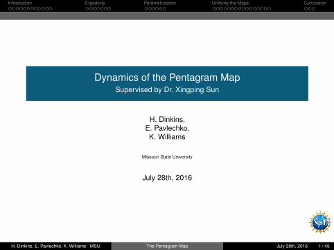
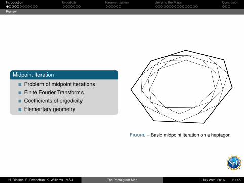
Midpoint Iteration
Problem of midpoint iterations
Finite Fourier Transforms
Coefficients of ergodicity
Elementary geometry
FIGURE – Basic midpoint iteration on a heptagon
H. Dinkins, E. Pavlechko, K. Williams MSU The Pentagram Map July 28th, 2016 2 / 45

Introduction Ergodicity Parametrization Unifying the Maps Conclusion
Review
Midpoint Iteration
Problem of midpoint iterations
Finite Fourier Transforms
Coefficients of ergodicity
Elementary geometry
FIGURE – Basic midpoint iteration on a heptagon
H. Dinkins, E. Pavlechko, K. Williams MSU The Pentagram Map July 28th, 2016 2 / 45
Introduction Ergodicity Parametrization Unifying the Maps Conclusion
Review
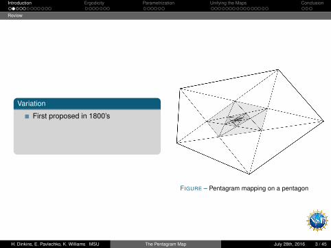
Variation
First proposed in 1800’s
Solved using Brouwer’s fixed pointtheorem
Projective geometry
FIGURE – Pentagram mapping on a pentagon
H. Dinkins, E. Pavlechko, K. Williams MSU The Pentagram Map July 28th, 2016 3 / 45
Introduction Ergodicity Parametrization Unifying the Maps Conclusion
Review
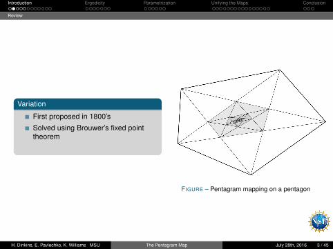
Variation
First proposed in 1800’s
Solved using Brouwer’s fixed pointtheorem
Projective geometry
FIGURE – Pentagram mapping on a pentagon
H. Dinkins, E. Pavlechko, K. Williams MSU The Pentagram Map July 28th, 2016 3 / 45
Introduction Ergodicity Parametrization Unifying the Maps Conclusion
Review
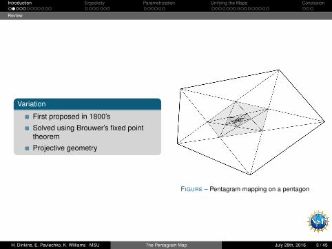
Variation
First proposed in 1800’s
Solved using Brouwer’s fixed pointtheorem
Projective geometry
FIGURE – Pentagram mapping on a pentagon
H. Dinkins, E. Pavlechko, K. Williams MSU The Pentagram Map July 28th, 2016 3 / 45
Introduction Ergodicity Parametrization Unifying the Maps Conclusion
Review
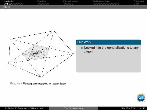
FIGURE – Pentagram mapping on a pentagon
Our Work
Looked into the generalizations to anyn-gon
Shown that the max rate of areadecrease for any pentagon is 14/15
Proved convergence for any regularn-gon
H. Dinkins, E. Pavlechko, K. Williams MSU The Pentagram Map July 28th, 2016 4 / 45
Introduction Ergodicity Parametrization Unifying the Maps Conclusion
Review
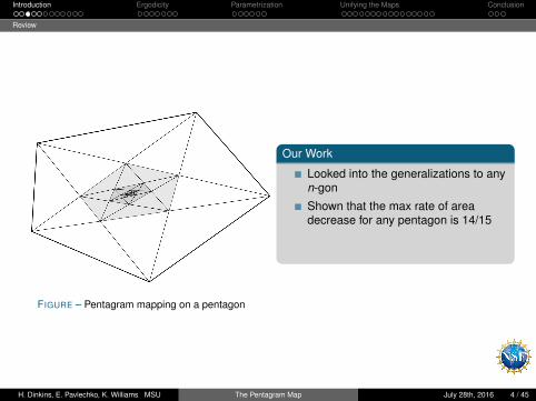
FIGURE – Pentagram mapping on a pentagon
Our Work
Looked into the generalizations to anyn-gon
Shown that the max rate of areadecrease for any pentagon is 14/15
Proved convergence for any regularn-gon
H. Dinkins, E. Pavlechko, K. Williams MSU The Pentagram Map July 28th, 2016 4 / 45
Introduction Ergodicity Parametrization Unifying the Maps Conclusion
Review
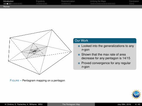
FIGURE – Pentagram mapping on a pentagon
Our Work
Looked into the generalizations to anyn-gon
Shown that the max rate of areadecrease for any pentagon is 14/15
Proved convergence for any regularn-gon
H. Dinkins, E. Pavlechko, K. Williams MSU The Pentagram Map July 28th, 2016 4 / 45
Introduction Ergodicity Parametrization Unifying the Maps Conclusion
Review
Midterm Goals
Generalize the pentagon’s area method to n-gons
Show the area method converges to a point
Use the matrices to prove convergence of vertices
Explore connections to projective geometry
H. Dinkins, E. Pavlechko, K. Williams MSU The Pentagram Map July 28th, 2016 5 / 45
Introduction Ergodicity Parametrization Unifying the Maps Conclusion
Review
Contents
1 IntroductionReviewExtending Previous Results
2 ErgodicityCoefficients of Ergodicity
3 ParametrizationSet-upLinear TransformationPython Program
4 Unifying the MapsConstructionBasic Properties of the MapRegular Polygon CaseGeneral PolygonsThe Pentagon Case
5 Conclusion
H. Dinkins, E. Pavlechko, K. Williams MSU The Pentagram Map July 28th, 2016 6 / 45
Introduction Ergodicity Parametrization Unifying the Maps Conclusion
Extending Previous Results
Schwartz’s Proof
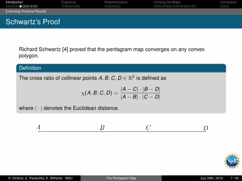
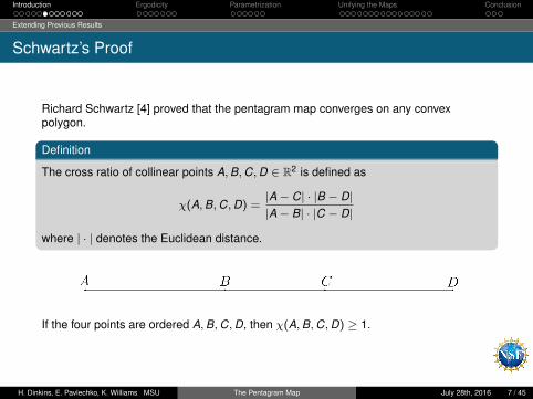
Richard Schwartz [4] proved that the pentagram map converges on any convexpolygon.
Definition
The cross ratio of collinear points A,B,C,D ∈ R2 is defined as
χ(A,B,C,D) =|A− C| · |B − D||A− B| · |C − D|
where | · | denotes the Euclidean distance.
If the four points are ordered A,B,C,D, then χ(A,B,C,D) ≥ 1.
H. Dinkins, E. Pavlechko, K. Williams MSU The Pentagram Map July 28th, 2016 7 / 45
Introduction Ergodicity Parametrization Unifying the Maps Conclusion
Extending Previous Results
Schwartz’s Proof
Definition
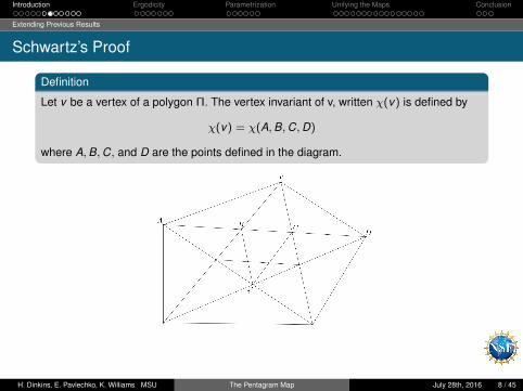
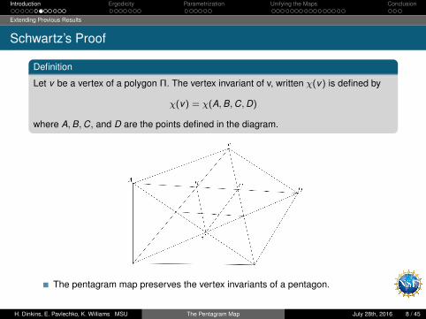
Let v be a vertex of a polygon Π. The vertex invariant of v, written χ(v) is defined by
χ(v) = χ(A,B,C,D)
where A,B,C, and D are the points defined in the diagram.
The pentagram map preserves the vertex invariants of a pentagon.The pentagram map preserves the product of the vertex invariants for anypolygon.
H. Dinkins, E. Pavlechko, K. Williams MSU The Pentagram Map July 28th, 2016 8 / 45
Introduction Ergodicity Parametrization Unifying the Maps Conclusion
Extending Previous Results
Schwartz’s Proof
Definition
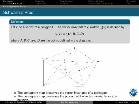
Let v be a vertex of a polygon Π. The vertex invariant of v, written χ(v) is defined by
χ(v) = χ(A,B,C,D)
where A,B,C, and D are the points defined in the diagram.
The pentagram map preserves the vertex invariants of a pentagon.
The pentagram map preserves the product of the vertex invariants for anypolygon.
H. Dinkins, E. Pavlechko, K. Williams MSU The Pentagram Map July 28th, 2016 8 / 45
Introduction Ergodicity Parametrization Unifying the Maps Conclusion
Extending Previous Results
Schwartz’s Proof
Definition
Let v be a vertex of a polygon Π. The vertex invariant of v, written χ(v) is defined by
χ(v) = χ(A,B,C,D)
where A,B,C, and D are the points defined in the diagram.
The pentagram map preserves the vertex invariants of a pentagon.The pentagram map preserves the product of the vertex invariants for anypolygon.
H. Dinkins, E. Pavlechko, K. Williams MSU The Pentagram Map July 28th, 2016 8 / 45
Introduction Ergodicity Parametrization Unifying the Maps Conclusion
Extending Previous Results
Schwartz’s Proof
Definition
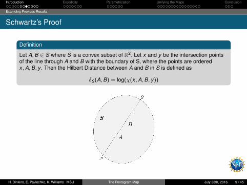
Let A,B ∈ S where S is a convex subset of R2. Let x and y be the intersection pointsof the line through A and B with the boundary of S, where the points are orderedx ,A,B, y . Then the Hilbert Distance between A and B in S is defined as
δS(A,B) = log(χ(x ,A,B, y))
H. Dinkins, E. Pavlechko, K. Williams MSU The Pentagram Map July 28th, 2016 9 / 45
Introduction Ergodicity Parametrization Unifying the Maps Conclusion
Extending Previous Results
Schwartz’s Proof
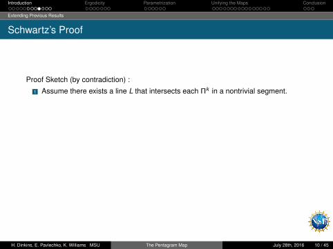
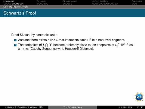
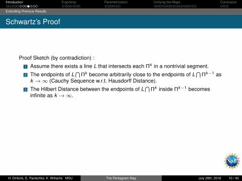
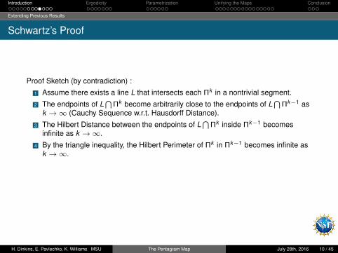
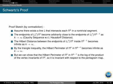
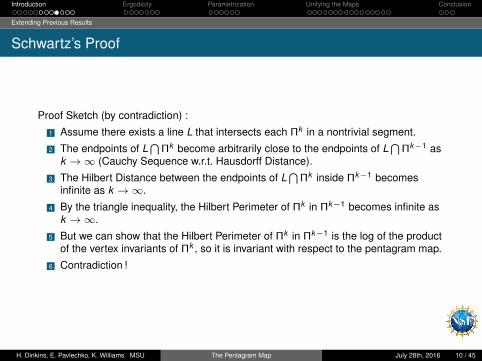
Proof Sketch (by contradiction) :
1 Assume there exists a line L that intersects each Πk in a nontrivial segment.
2 The endpoints of L⋂
Πk become arbitrarily close to the endpoints of L⋂
Πk−1 ask →∞ (Cauchy Sequence w.r.t. Hausdorff Distance).
3 The Hilbert Distance between the endpoints of L⋂
Πk inside Πk−1 becomesinfinite as k →∞.
4 By the triangle inequality, the Hilbert Perimeter of Πk in Πk−1 becomes infinite ask →∞.
5 But we can show that the Hilbert Perimeter of Πk in Πk−1 is the log of the productof the vertex invariants of Πk , so it is invariant with respect to the pentagram map.
6 Contradiction !
H. Dinkins, E. Pavlechko, K. Williams MSU The Pentagram Map July 28th, 2016 10 / 45
Introduction Ergodicity Parametrization Unifying the Maps Conclusion
Extending Previous Results
Schwartz’s Proof
Proof Sketch (by contradiction) :
1 Assume there exists a line L that intersects each Πk in a nontrivial segment.
2 The endpoints of L⋂
Πk become arbitrarily close to the endpoints of L⋂
Πk−1 ask →∞ (Cauchy Sequence w.r.t. Hausdorff Distance).
3 The Hilbert Distance between the endpoints of L⋂
Πk inside Πk−1 becomesinfinite as k →∞.
4 By the triangle inequality, the Hilbert Perimeter of Πk in Πk−1 becomes infinite ask →∞.
5 But we can show that the Hilbert Perimeter of Πk in Πk−1 is the log of the productof the vertex invariants of Πk , so it is invariant with respect to the pentagram map.
6 Contradiction !
H. Dinkins, E. Pavlechko, K. Williams MSU The Pentagram Map July 28th, 2016 10 / 45
Introduction Ergodicity Parametrization Unifying the Maps Conclusion
Extending Previous Results
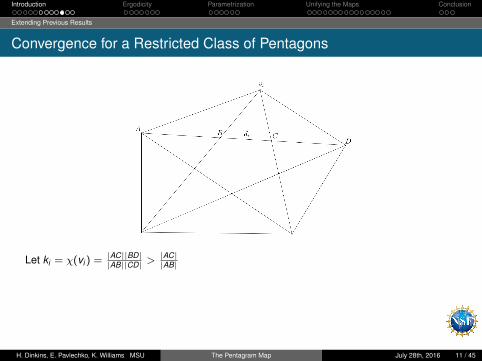
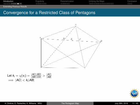
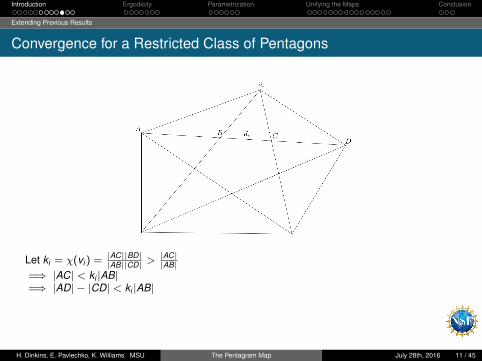
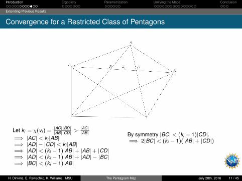
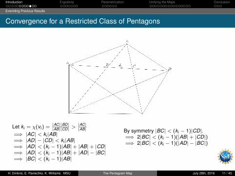
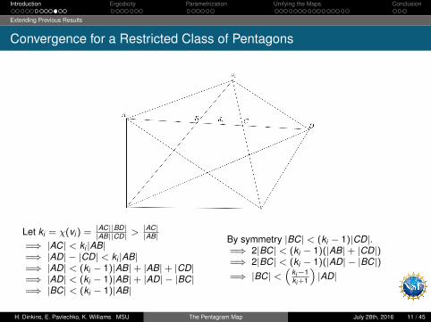
Convergence for a Restricted Class of Pentagons
Let ki = χ(vi ) = |AC||BD||AB||CD| >
|AC||AB|
=⇒ |AC| < ki |AB|=⇒ |AD| − |CD| < ki |AB|=⇒ |AD| < (ki − 1)|AB|+ |AB|+ |CD|=⇒ |AD| < (ki − 1)|AB|+ |AD| − |BC|=⇒ |BC| < (ki − 1)|AB|
By symmetry |BC| < (ki − 1)|CD|.=⇒ 2|BC| < (ki − 1)(|AB|+ |CD|)=⇒ 2|BC| < (ki − 1)(|AD| − |BC|)=⇒ |BC| <
(ki−1ki +1
)|AD|
H. Dinkins, E. Pavlechko, K. Williams MSU The Pentagram Map July 28th, 2016 11 / 45
Introduction Ergodicity Parametrization Unifying the Maps Conclusion
Extending Previous Results
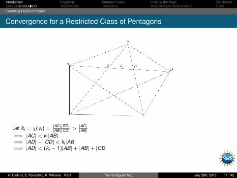
Convergence for a Restricted Class of Pentagons
Let ki = χ(vi ) = |AC||BD||AB||CD| >
|AC||AB|
=⇒ |AC| < ki |AB|
=⇒ |AD| − |CD| < ki |AB|=⇒ |AD| < (ki − 1)|AB|+ |AB|+ |CD|=⇒ |AD| < (ki − 1)|AB|+ |AD| − |BC|=⇒ |BC| < (ki − 1)|AB|
By symmetry |BC| < (ki − 1)|CD|.=⇒ 2|BC| < (ki − 1)(|AB|+ |CD|)=⇒ 2|BC| < (ki − 1)(|AD| − |BC|)=⇒ |BC| <
(ki−1ki +1
)|AD|
H. Dinkins, E. Pavlechko, K. Williams MSU The Pentagram Map July 28th, 2016 11 / 45
Introduction Ergodicity Parametrization Unifying the Maps Conclusion
Extending Previous Results
Convergence for a Restricted Class of Pentagons
Let ki = χ(vi ) = |AC||BD||AB||CD| >
|AC||AB|
=⇒ |AC| < ki |AB|=⇒ |AD| − |CD| < ki |AB|
=⇒ |AD| < (ki − 1)|AB|+ |AB|+ |CD|=⇒ |AD| < (ki − 1)|AB|+ |AD| − |BC|=⇒ |BC| < (ki − 1)|AB|
By symmetry |BC| < (ki − 1)|CD|.=⇒ 2|BC| < (ki − 1)(|AB|+ |CD|)=⇒ 2|BC| < (ki − 1)(|AD| − |BC|)=⇒ |BC| <
(ki−1ki +1
)|AD|
H. Dinkins, E. Pavlechko, K. Williams MSU The Pentagram Map July 28th, 2016 11 / 45
Introduction Ergodicity Parametrization Unifying the Maps Conclusion
Extending Previous Results
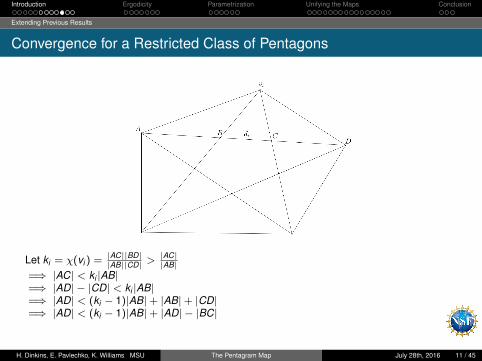
Convergence for a Restricted Class of Pentagons
Let ki = χ(vi ) = |AC||BD||AB||CD| >
|AC||AB|
=⇒ |AC| < ki |AB|=⇒ |AD| − |CD| < ki |AB|=⇒ |AD| < (ki − 1)|AB|+ |AB|+ |CD|
=⇒ |AD| < (ki − 1)|AB|+ |AD| − |BC|=⇒ |BC| < (ki − 1)|AB|
By symmetry |BC| < (ki − 1)|CD|.=⇒ 2|BC| < (ki − 1)(|AB|+ |CD|)=⇒ 2|BC| < (ki − 1)(|AD| − |BC|)=⇒ |BC| <
(ki−1ki +1
)|AD|
H. Dinkins, E. Pavlechko, K. Williams MSU The Pentagram Map July 28th, 2016 11 / 45
Introduction Ergodicity Parametrization Unifying the Maps Conclusion
Extending Previous Results
Convergence for a Restricted Class of Pentagons
Let ki = χ(vi ) = |AC||BD||AB||CD| >
|AC||AB|
=⇒ |AC| < ki |AB|=⇒ |AD| − |CD| < ki |AB|=⇒ |AD| < (ki − 1)|AB|+ |AB|+ |CD|=⇒ |AD| < (ki − 1)|AB|+ |AD| − |BC|
=⇒ |BC| < (ki − 1)|AB|
By symmetry |BC| < (ki − 1)|CD|.=⇒ 2|BC| < (ki − 1)(|AB|+ |CD|)=⇒ 2|BC| < (ki − 1)(|AD| − |BC|)=⇒ |BC| <
(ki−1ki +1
)|AD|
H. Dinkins, E. Pavlechko, K. Williams MSU The Pentagram Map July 28th, 2016 11 / 45
Introduction Ergodicity Parametrization Unifying the Maps Conclusion
Extending Previous Results
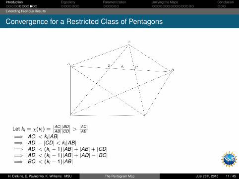
Convergence for a Restricted Class of Pentagons
Let ki = χ(vi ) = |AC||BD||AB||CD| >
|AC||AB|
=⇒ |AC| < ki |AB|=⇒ |AD| − |CD| < ki |AB|=⇒ |AD| < (ki − 1)|AB|+ |AB|+ |CD|=⇒ |AD| < (ki − 1)|AB|+ |AD| − |BC|=⇒ |BC| < (ki − 1)|AB|
By symmetry |BC| < (ki − 1)|CD|.=⇒ 2|BC| < (ki − 1)(|AB|+ |CD|)=⇒ 2|BC| < (ki − 1)(|AD| − |BC|)=⇒ |BC| <
(ki−1ki +1
)|AD|
H. Dinkins, E. Pavlechko, K. Williams MSU The Pentagram Map July 28th, 2016 11 / 45

Introduction Ergodicity Parametrization Unifying the Maps Conclusion
Extending Previous Results
Convergence for a Restricted Class of Pentagons
Let ki = χ(vi ) = |AC||BD||AB||CD| >
|AC||AB|
=⇒ |AC| < ki |AB|=⇒ |AD| − |CD| < ki |AB|=⇒ |AD| < (ki − 1)|AB|+ |AB|+ |CD|=⇒ |AD| < (ki − 1)|AB|+ |AD| − |BC|=⇒ |BC| < (ki − 1)|AB|
By symmetry |BC| < (ki − 1)|CD|.
=⇒ 2|BC| < (ki − 1)(|AB|+ |CD|)=⇒ 2|BC| < (ki − 1)(|AD| − |BC|)=⇒ |BC| <
(ki−1ki +1
)|AD|
H. Dinkins, E. Pavlechko, K. Williams MSU The Pentagram Map July 28th, 2016 11 / 45
Introduction Ergodicity Parametrization Unifying the Maps Conclusion
Extending Previous Results
Convergence for a Restricted Class of Pentagons
Let ki = χ(vi ) = |AC||BD||AB||CD| >
|AC||AB|
=⇒ |AC| < ki |AB|=⇒ |AD| − |CD| < ki |AB|=⇒ |AD| < (ki − 1)|AB|+ |AB|+ |CD|=⇒ |AD| < (ki − 1)|AB|+ |AD| − |BC|=⇒ |BC| < (ki − 1)|AB|
By symmetry |BC| < (ki − 1)|CD|.=⇒ 2|BC| < (ki − 1)(|AB|+ |CD|)
=⇒ 2|BC| < (ki − 1)(|AD| − |BC|)=⇒ |BC| <
(ki−1ki +1
)|AD|
H. Dinkins, E. Pavlechko, K. Williams MSU The Pentagram Map July 28th, 2016 11 / 45
Introduction Ergodicity Parametrization Unifying the Maps Conclusion
Extending Previous Results
Convergence for a Restricted Class of Pentagons
Let ki = χ(vi ) = |AC||BD||AB||CD| >
|AC||AB|
=⇒ |AC| < ki |AB|=⇒ |AD| − |CD| < ki |AB|=⇒ |AD| < (ki − 1)|AB|+ |AB|+ |CD|=⇒ |AD| < (ki − 1)|AB|+ |AD| − |BC|=⇒ |BC| < (ki − 1)|AB|
By symmetry |BC| < (ki − 1)|CD|.=⇒ 2|BC| < (ki − 1)(|AB|+ |CD|)=⇒ 2|BC| < (ki − 1)(|AD| − |BC|)
=⇒ |BC| <(
ki−1ki +1
)|AD|
H. Dinkins, E. Pavlechko, K. Williams MSU The Pentagram Map July 28th, 2016 11 / 45
Introduction Ergodicity Parametrization Unifying the Maps Conclusion
Extending Previous Results
Convergence for a Restricted Class of Pentagons
Let ki = χ(vi ) = |AC||BD||AB||CD| >
|AC||AB|
=⇒ |AC| < ki |AB|=⇒ |AD| − |CD| < ki |AB|=⇒ |AD| < (ki − 1)|AB|+ |AB|+ |CD|=⇒ |AD| < (ki − 1)|AB|+ |AD| − |BC|=⇒ |BC| < (ki − 1)|AB|
By symmetry |BC| < (ki − 1)|CD|.=⇒ 2|BC| < (ki − 1)(|AB|+ |CD|)=⇒ 2|BC| < (ki − 1)(|AD| − |BC|)=⇒ |BC| <
(ki−1ki +1
)|AD|
H. Dinkins, E. Pavlechko, K. Williams MSU The Pentagram Map July 28th, 2016 11 / 45
Introduction Ergodicity Parametrization Unifying the Maps Conclusion
Extending Previous Results
Convergence for a Restricted Class of Pentagons
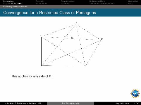
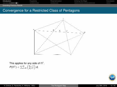
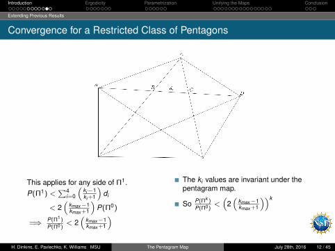
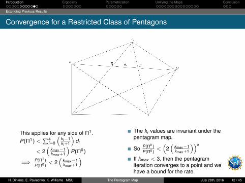
This applies for any side of Π1.
P(Π1) <∑4
i=0
(ki−1ki +1
)di
< 2(
kmax−1kmax +1
)P(Π0)
=⇒ P(Π1)
P(Π0)< 2
(kmax−1kmax +1
)
The ki values are invariant under thepentagram map.
So P(Πk )
P(Π0)<(
2(
kmax−1kmax +1
))k
If kmax < 3, then the pentagramiteration converges to a point and wehave a bound for the rate.
H. Dinkins, E. Pavlechko, K. Williams MSU The Pentagram Map July 28th, 2016 12 / 45
Introduction Ergodicity Parametrization Unifying the Maps Conclusion
Extending Previous Results
Convergence for a Restricted Class of Pentagons
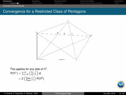
This applies for any side of Π1.P(Π1) <
∑4i=0
(ki−1ki +1
)di
< 2(
kmax−1kmax +1
)P(Π0)
=⇒ P(Π1)
P(Π0)< 2
(kmax−1kmax +1
)
The ki values are invariant under thepentagram map.
So P(Πk )
P(Π0)<(
2(
kmax−1kmax +1
))k
If kmax < 3, then the pentagramiteration converges to a point and wehave a bound for the rate.
H. Dinkins, E. Pavlechko, K. Williams MSU The Pentagram Map July 28th, 2016 12 / 45
Introduction Ergodicity Parametrization Unifying the Maps Conclusion
Extending Previous Results
Convergence for a Restricted Class of Pentagons
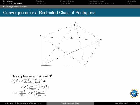
This applies for any side of Π1.P(Π1) <
∑4i=0
(ki−1ki +1
)di
< 2(
kmax−1kmax +1
)P(Π0)
=⇒ P(Π1)
P(Π0)< 2
(kmax−1kmax +1
)
The ki values are invariant under thepentagram map.
So P(Πk )
P(Π0)<(
2(
kmax−1kmax +1
))k
If kmax < 3, then the pentagramiteration converges to a point and wehave a bound for the rate.
H. Dinkins, E. Pavlechko, K. Williams MSU The Pentagram Map July 28th, 2016 12 / 45
Introduction Ergodicity Parametrization Unifying the Maps Conclusion
Extending Previous Results
Convergence for a Restricted Class of Pentagons
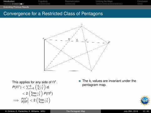
This applies for any side of Π1.P(Π1) <
∑4i=0
(ki−1ki +1
)di
< 2(
kmax−1kmax +1
)P(Π0)
=⇒ P(Π1)
P(Π0)< 2
(kmax−1kmax +1
)
The ki values are invariant under thepentagram map.
So P(Πk )
P(Π0)<(
2(
kmax−1kmax +1
))k
If kmax < 3, then the pentagramiteration converges to a point and wehave a bound for the rate.
H. Dinkins, E. Pavlechko, K. Williams MSU The Pentagram Map July 28th, 2016 12 / 45
Introduction Ergodicity Parametrization Unifying the Maps Conclusion
Extending Previous Results
Convergence for a Restricted Class of Pentagons
This applies for any side of Π1.P(Π1) <
∑4i=0
(ki−1ki +1
)di
< 2(
kmax−1kmax +1
)P(Π0)
=⇒ P(Π1)
P(Π0)< 2
(kmax−1kmax +1
)
The ki values are invariant under thepentagram map.
So P(Πk )
P(Π0)<(
2(
kmax−1kmax +1
))k
If kmax < 3, then the pentagramiteration converges to a point and wehave a bound for the rate.
H. Dinkins, E. Pavlechko, K. Williams MSU The Pentagram Map July 28th, 2016 12 / 45
Introduction Ergodicity Parametrization Unifying the Maps Conclusion
Extending Previous Results
A Conjecture
Explorations in geogebra indicate that P(Π1)
P(Π0)< kmax−1
kmax +1 holds in general for anypolygon, regardless of the number of sides, but we have not been able to prove this.
H. Dinkins, E. Pavlechko, K. Williams MSU The Pentagram Map July 28th, 2016 13 / 45
Introduction Ergodicity Parametrization Unifying the Maps Conclusion
Coefficients of Ergodicity
Representation by matrices
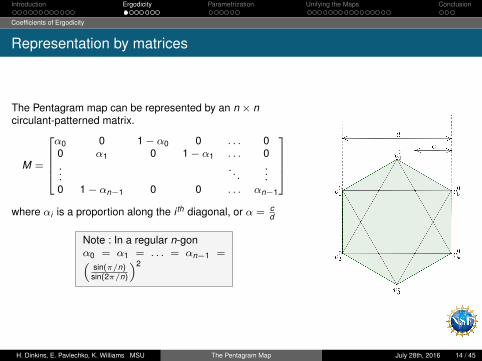
The Pentagram map can be represented by an n × ncirculant-patterned matrix.
M =
α0 0 1− α0 0 . . . 00 α1 0 1− α1 . . . 0...
. . ....
0 1− αn−1 0 0 . . . αn−1
where αi is a proportion along the i th diagonal, or α = c
d
Note : In a regular n-gonα0 = α1 = . . . = αn−1 =(
sin(π/n)sin(2π/n)
)2
H. Dinkins, E. Pavlechko, K. Williams MSU The Pentagram Map July 28th, 2016 14 / 45

Introduction Ergodicity Parametrization Unifying the Maps Conclusion
Coefficients of Ergodicity
Matrices continued
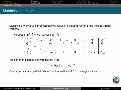
Multiplying M by a vector of vertices will result in a column vector of the next polygon’svertices
vertices of Πk+1 = Mk (vertices of Πk )vk+1
0vk+1
1...
vk+1n−1
=
α0 0 1− α0 0 . . . 00 α1 0 1− α1 . . . 0...
. . ....
0 1− αn−1 0 0 . . . αn−1
vk0
vk1...
vkn−1
We can then express the vertices of Πk as
Πk = Mk Mk−1 . . .M0Π0
Our project’s main goal is to show that the vertices of Πk converge as k →∞
H. Dinkins, E. Pavlechko, K. Williams MSU The Pentagram Map July 28th, 2016 15 / 45
Introduction Ergodicity Parametrization Unifying the Maps Conclusion
Coefficients of Ergodicity
Matrices continued
Multiplying M by a vector of vertices will result in a column vector of the next polygon’svertices
vertices of Πk+1 = Mk (vertices of Πk )vk+1
0vk+1
1...
vk+1n−1
=
α0 0 1− α0 0 . . . 00 α1 0 1− α1 . . . 0...
. . ....
0 1− αn−1 0 0 . . . αn−1
vk0
vk1...
vkn−1
We can then express the vertices of Πk as
Πk = Mk Mk−1 . . .M0Π0
Our project’s main goal is to show that the vertices of Πk converge as k →∞
H. Dinkins, E. Pavlechko, K. Williams MSU The Pentagram Map July 28th, 2016 15 / 45
Introduction Ergodicity Parametrization Unifying the Maps Conclusion
Coefficients of Ergodicity
Past Uses
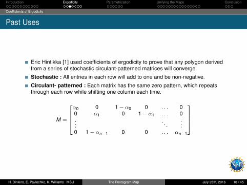
Eric Hintikka [1] used coefficients of ergodicity to prove that any polygon derivedfrom a series of stochastic circulant-patterned matrices will converge.
Stochastic : All entries in each row will add to one and be non-negative.
Circulant- patterned : Each matrix has the same zero pattern, which repeatsthrough each row while shifting one column each time.
M =
α0 0 1− α0 0 . . . 00 α1 0 1− α1 . . . 0...
. . ....
0 1− αn−1 0 0 . . . αn−1
H. Dinkins, E. Pavlechko, K. Williams MSU The Pentagram Map July 28th, 2016 16 / 45
Introduction Ergodicity Parametrization Unifying the Maps Conclusion
Coefficients of Ergodicity
Coefficients of Ergodicity
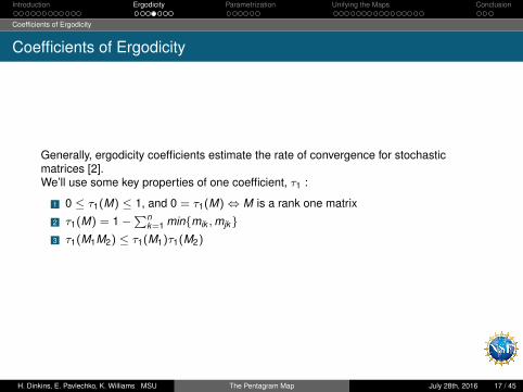
Generally, ergodicity coefficients estimate the rate of convergence for stochasticmatrices [2].We’ll use some key properties of one coefficient, τ1 :
1 0 ≤ τ1(M) ≤ 1, and 0 = τ1(M)⇔ M is a rank one matrix
2 τ1(M) = 1−∑n
k=1 min{mik ,mjk}3 τ1(M1M2) ≤ τ1(M1)τ1(M2)
H. Dinkins, E. Pavlechko, K. Williams MSU The Pentagram Map July 28th, 2016 17 / 45
Introduction Ergodicity Parametrization Unifying the Maps Conclusion
Coefficients of Ergodicity
Proving Convergence
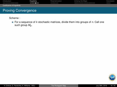
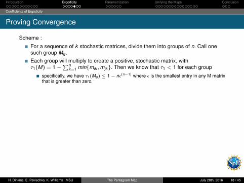
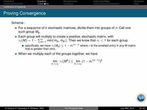
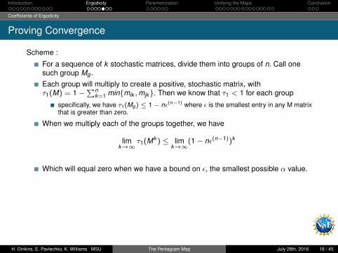
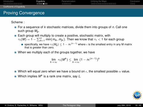
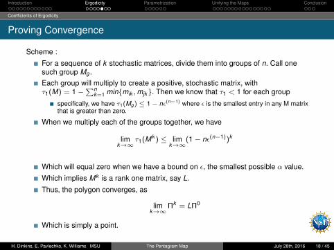
Scheme :
For a sequence of k stochastic matrices, divide them into groups of n. Call onesuch group Mg .
Each group will multiply to create a positive, stochastic matrix, withτ1(M) = 1−
∑nk=1 min{mik ,mjk}. Then we know that τ1 < 1 for each group
specifically, we have τ1(Mg) ≤ 1 − nε(n−1) where ε is the smallest entry in any M matrixthat is greater than zero.
When we multiply each of the groups together, we have
limk→∞
τ1(Mk ) ≤ limk→∞
(1− nε(n−1))k
Which will equal zero when we have a bound on ε, the smallest possible α value.
Which implies Mk is a rank one matrix, say L.
Thus, the polygon converges, as
limk→∞
Πk = LΠ0
Which is simply a point.
H. Dinkins, E. Pavlechko, K. Williams MSU The Pentagram Map July 28th, 2016 18 / 45
Introduction Ergodicity Parametrization Unifying the Maps Conclusion
Coefficients of Ergodicity
Proving Convergence
Scheme :
For a sequence of k stochastic matrices, divide them into groups of n. Call onesuch group Mg .Each group will multiply to create a positive, stochastic matrix, withτ1(M) = 1−
∑nk=1 min{mik ,mjk}. Then we know that τ1 < 1 for each group
specifically, we have τ1(Mg) ≤ 1 − nε(n−1) where ε is the smallest entry in any M matrixthat is greater than zero.
When we multiply each of the groups together, we have
limk→∞
τ1(Mk ) ≤ limk→∞
(1− nε(n−1))k
Which will equal zero when we have a bound on ε, the smallest possible α value.
Which implies Mk is a rank one matrix, say L.
Thus, the polygon converges, as
limk→∞
Πk = LΠ0
Which is simply a point.
H. Dinkins, E. Pavlechko, K. Williams MSU The Pentagram Map July 28th, 2016 18 / 45
Introduction Ergodicity Parametrization Unifying the Maps Conclusion
Coefficients of Ergodicity
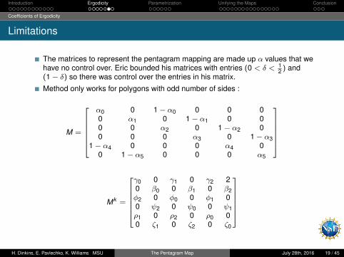
Limitations
The matrices to represent the pentagram mapping are made up α values that wehave no control over. Eric bounded his matrices with entries (0 < δ < 1
2 ) and(1− δ) so there was control over the entries in his matrix.
Method only works for polygons with odd number of sides :
M =
α0 0 1− α0 0 0 00 α1 0 1− α1 0 00 0 α2 0 1− α2 00 0 0 α3 0 1− α3
1− α4 0 0 0 α4 00 1− α5 0 0 0 α5
Mk =
γ0 0 γ1 0 γ2 20 β0 0 β1 0 β2φ2 0 φ0 0 φ1 00 ψ2 0 ψ0 0 ψ1ρ1 0 ρ2 0 ρ0 00 ζ1 0 ζ2 0 ζ0
H. Dinkins, E. Pavlechko, K. Williams MSU The Pentagram Map July 28th, 2016 19 / 45
Introduction Ergodicity Parametrization Unifying the Maps Conclusion
Coefficients of Ergodicity
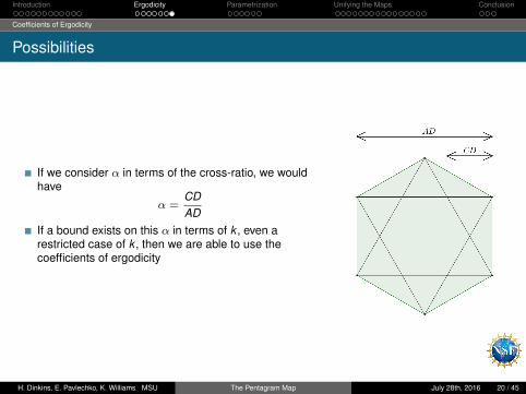
Possibilities
If we consider α in terms of the cross-ratio, we wouldhave
α =CDAD
If a bound exists on this α in terms of k , even arestricted case of k , then we are able to use thecoefficients of ergodicity
H. Dinkins, E. Pavlechko, K. Williams MSU The Pentagram Map July 28th, 2016 20 / 45
Introduction Ergodicity Parametrization Unifying the Maps Conclusion
Set-up
Set-up
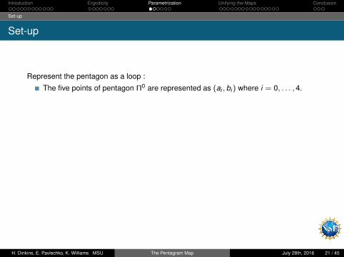
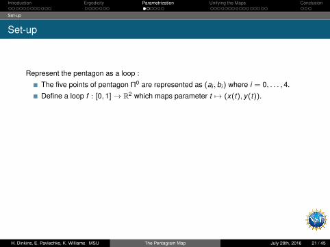
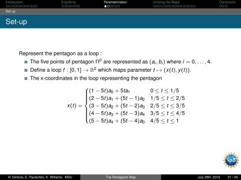
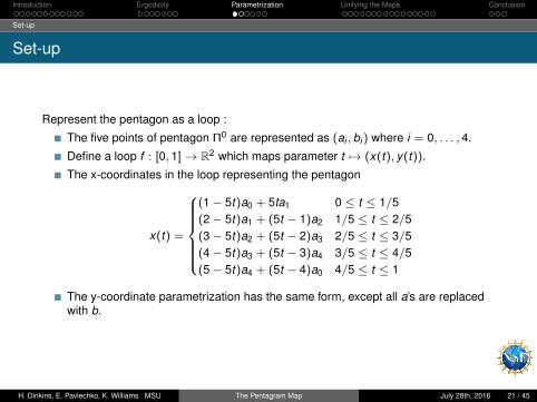
Represent the pentagon as a loop :
The five points of pentagon Π0 are represented as (ai , bi ) where i = 0, . . . , 4.
Define a loop f : [0, 1]→ R2 which maps parameter t 7→ (x(t), y(t)).
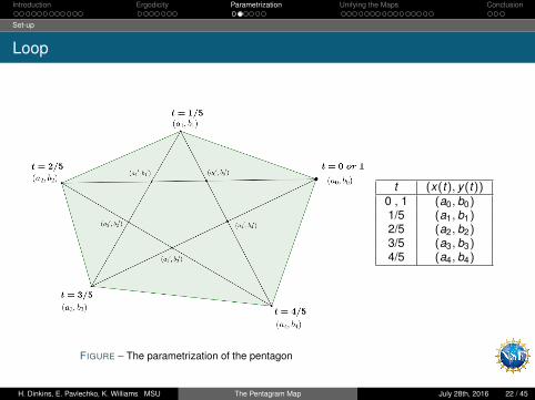
The x-coordinates in the loop representing the pentagon
x(t) =
(1− 5t)a0 + 5ta1 0 ≤ t ≤ 1/5(2− 5t)a1 + (5t − 1)a2 1/5 ≤ t ≤ 2/5(3− 5t)a2 + (5t − 2)a3 2/5 ≤ t ≤ 3/5(4− 5t)a3 + (5t − 3)a4 3/5 ≤ t ≤ 4/5(5− 5t)a4 + (5t − 4)a0 4/5 ≤ t ≤ 1
The y-coordinate parametrization has the same form, except all a’s are replacedwith b.
H. Dinkins, E. Pavlechko, K. Williams MSU The Pentagram Map July 28th, 2016 21 / 45
Introduction Ergodicity Parametrization Unifying the Maps Conclusion
Set-up
Set-up
Represent the pentagon as a loop :
The five points of pentagon Π0 are represented as (ai , bi ) where i = 0, . . . , 4.
Define a loop f : [0, 1]→ R2 which maps parameter t 7→ (x(t), y(t)).
The x-coordinates in the loop representing the pentagon
x(t) =
(1− 5t)a0 + 5ta1 0 ≤ t ≤ 1/5(2− 5t)a1 + (5t − 1)a2 1/5 ≤ t ≤ 2/5(3− 5t)a2 + (5t − 2)a3 2/5 ≤ t ≤ 3/5(4− 5t)a3 + (5t − 3)a4 3/5 ≤ t ≤ 4/5(5− 5t)a4 + (5t − 4)a0 4/5 ≤ t ≤ 1
The y-coordinate parametrization has the same form, except all a’s are replacedwith b.
H. Dinkins, E. Pavlechko, K. Williams MSU The Pentagram Map July 28th, 2016 21 / 45
Introduction Ergodicity Parametrization Unifying the Maps Conclusion
Set-up
Loop
FIGURE – The parametrization of the pentagon
t (x(t), y(t))0 , 1 (a0, b0)1/5 (a1, b1)2/5 (a2, b2)3/5 (a3, b3)4/5 (a4, b4)
H. Dinkins, E. Pavlechko, K. Williams MSU The Pentagram Map July 28th, 2016 22 / 45
Introduction Ergodicity Parametrization Unifying the Maps Conclusion
Linear Transformation
Moving Segments
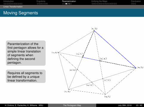
Paramterization of thefirst pentagon allows for asimple linear translationof segments whendefining the secondpentagon.
Requires all segments tobe defined by a uniquelinear transformation.
H. Dinkins, E. Pavlechko, K. Williams MSU The Pentagram Map July 28th, 2016 23 / 45
Introduction Ergodicity Parametrization Unifying the Maps Conclusion
Linear Transformation
Matrix Multiplication
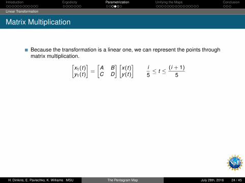
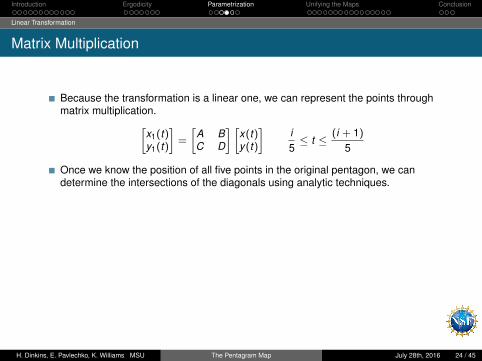
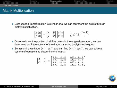
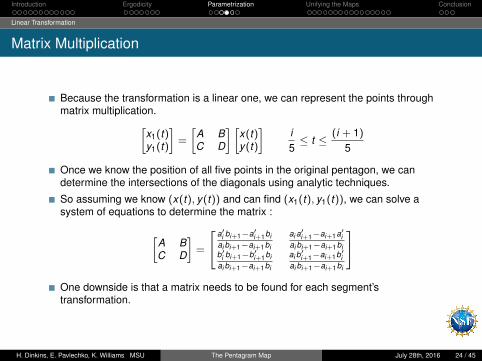
Because the transformation is a linear one, we can represent the points throughmatrix multiplication.[
x1(t)y1(t)
]=
[A BC D
] [x(t)y(t)
]i5≤ t ≤
(i + 1)
5
Once we know the position of all five points in the original pentagon, we candetermine the intersections of the diagonals using analytic techniques.
So assuming we know (x(t), y(t)) and can find (x1(t), y1(t)), we can solve asystem of equations to determine the matrix :
[A BC D
]=
a′i bi+1−a′i+1biai bi+1−ai+1bi
ai a′i+1−ai+1a′i
ai bi+1−ai+1bib′i bi+1−b′i+1biai bi+1−ai+1bi
ai b′i+1−ai+1b′i
ai bi+1−ai+1bi
One downside is that a matrix needs to be found for each segment’stransformation.
H. Dinkins, E. Pavlechko, K. Williams MSU The Pentagram Map July 28th, 2016 24 / 45
Introduction Ergodicity Parametrization Unifying the Maps Conclusion
Linear Transformation
Matrix Multiplication
Because the transformation is a linear one, we can represent the points throughmatrix multiplication.[
x1(t)y1(t)
]=
[A BC D
] [x(t)y(t)
]i5≤ t ≤
(i + 1)
5
Once we know the position of all five points in the original pentagon, we candetermine the intersections of the diagonals using analytic techniques.
So assuming we know (x(t), y(t)) and can find (x1(t), y1(t)), we can solve asystem of equations to determine the matrix :
[A BC D
]=
a′i bi+1−a′i+1biai bi+1−ai+1bi
ai a′i+1−ai+1a′i
ai bi+1−ai+1bib′i bi+1−b′i+1biai bi+1−ai+1bi
ai b′i+1−ai+1b′i
ai bi+1−ai+1bi
One downside is that a matrix needs to be found for each segment’stransformation.
H. Dinkins, E. Pavlechko, K. Williams MSU The Pentagram Map July 28th, 2016 24 / 45
Introduction Ergodicity Parametrization Unifying the Maps Conclusion
Linear Transformation
Finding Convergence
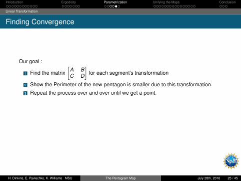
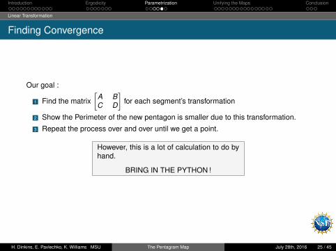
Our goal :
1 Find the matrix[
A BC D
]for each segment’s transformation
2 Show the Perimeter of the new pentagon is smaller due to this transformation.
3 Repeat the process over and over until we get a point.
However, this is a lot of calculation to do byhand.
BRING IN THE PYTHON !
H. Dinkins, E. Pavlechko, K. Williams MSU The Pentagram Map July 28th, 2016 25 / 45
Introduction Ergodicity Parametrization Unifying the Maps Conclusion
Linear Transformation
Finding Convergence
Our goal :
1 Find the matrix[
A BC D
]for each segment’s transformation
2 Show the Perimeter of the new pentagon is smaller due to this transformation.
3 Repeat the process over and over until we get a point.
However, this is a lot of calculation to do byhand.
BRING IN THE PYTHON !
H. Dinkins, E. Pavlechko, K. Williams MSU The Pentagram Map July 28th, 2016 25 / 45
Introduction Ergodicity Parametrization Unifying the Maps Conclusion
Python Program
The Game
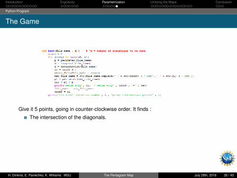
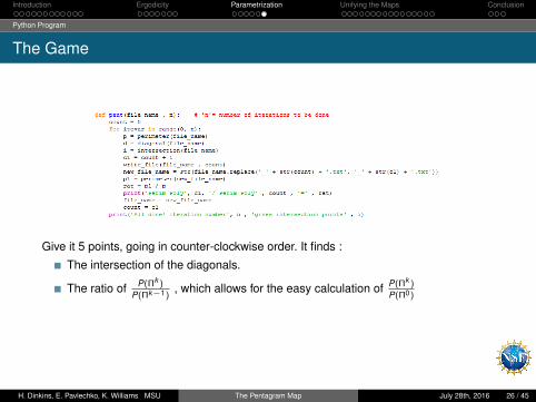
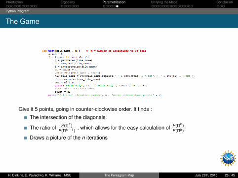
Give it 5 points, going in counter-clockwise order. It finds :
The intersection of the diagonals.
The ratio of P(Πk )
P(Πk−1), which allows for the easy calculation of P(Πk )
P(Π0)
Draws a picture of the n iterations
Gives the vertices of Πk
H. Dinkins, E. Pavlechko, K. Williams MSU The Pentagram Map July 28th, 2016 26 / 45
Introduction Ergodicity Parametrization Unifying the Maps Conclusion
Python Program
The Game
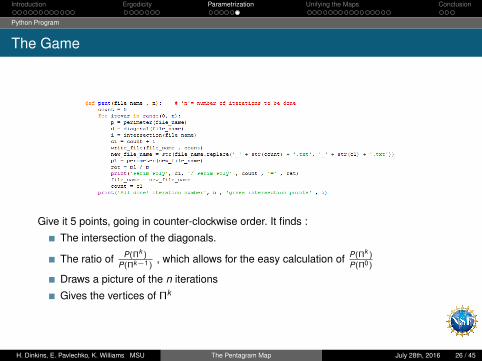
Give it 5 points, going in counter-clockwise order. It finds :
The intersection of the diagonals.
The ratio of P(Πk )
P(Πk−1), which allows for the easy calculation of P(Πk )
P(Π0)
Draws a picture of the n iterations
Gives the vertices of Πk
H. Dinkins, E. Pavlechko, K. Williams MSU The Pentagram Map July 28th, 2016 26 / 45
Introduction Ergodicity Parametrization Unifying the Maps Conclusion
Construction
Two Types of Maps
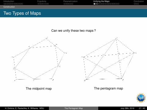
Can we unify these two maps ?
The midpoint map The pentagram map
H. Dinkins, E. Pavlechko, K. Williams MSU The Pentagram Map July 28th, 2016 27 / 45
Introduction Ergodicity Parametrization Unifying the Maps Conclusion
Construction
The Generalized Pentagram Map (GPM)
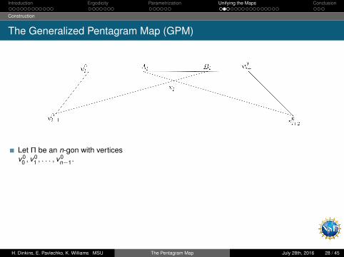
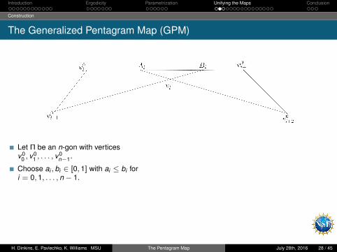
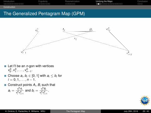
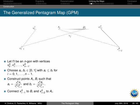
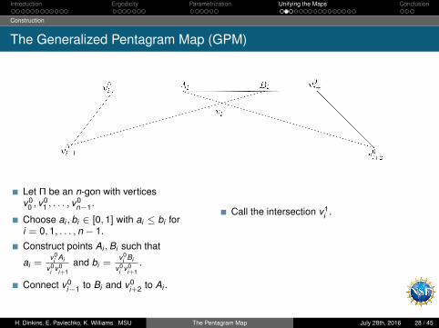
Let Π be an n-gon with verticesv0
0 , v01 , . . . , v
0n−1.
Choose ai , bi ∈ [0, 1] with ai ≤ bi fori = 0, 1, . . . , n − 1.
Construct points Ai ,Bi such that
ai =v0
i Aiv0
i v0i+1
and bi =v0
i Biv0
i v0i+1
.
Connect v0i−1 to Bi and v0
i+2 to Ai .
Call the intersection v1i .
Apply this process to each edge to form thevertices of an n-gon T (Π).
Applying this process k times gives usT k (Π).
H. Dinkins, E. Pavlechko, K. Williams MSU The Pentagram Map July 28th, 2016 28 / 45
Introduction Ergodicity Parametrization Unifying the Maps Conclusion
Construction
The Generalized Pentagram Map (GPM)
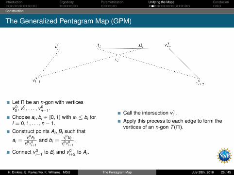
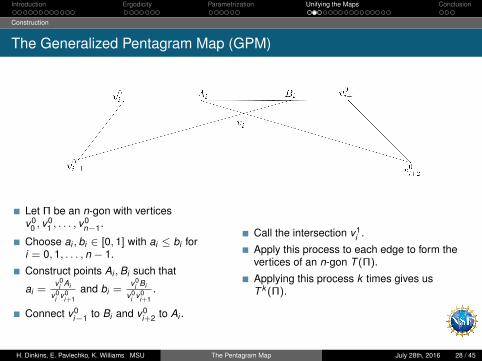
Let Π be an n-gon with verticesv0
0 , v01 , . . . , v
0n−1.
Choose ai , bi ∈ [0, 1] with ai ≤ bi fori = 0, 1, . . . , n − 1.
Construct points Ai ,Bi such that
ai =v0
i Aiv0
i v0i+1
and bi =v0
i Biv0
i v0i+1
.
Connect v0i−1 to Bi and v0
i+2 to Ai .
Call the intersection v1i .
Apply this process to each edge to form thevertices of an n-gon T (Π).
Applying this process k times gives usT k (Π).
H. Dinkins, E. Pavlechko, K. Williams MSU The Pentagram Map July 28th, 2016 28 / 45
Introduction Ergodicity Parametrization Unifying the Maps Conclusion
Construction
Representing the Map
A GPM T is uniquely determined by the ai and bi values.
Let f (T ) = (a0, b0, a1, b1, . . . , an−1, bn−1).
H. Dinkins, E. Pavlechko, K. Williams MSU The Pentagram Map July 28th, 2016 29 / 45
Introduction Ergodicity Parametrization Unifying the Maps Conclusion
Construction
Representing the Map
A GPM T is uniquely determined by the ai and bi values.
Let f (T ) = (a0, b0, a1, b1, . . . , an−1, bn−1).
H. Dinkins, E. Pavlechko, K. Williams MSU The Pentagram Map July 28th, 2016 29 / 45
Introduction Ergodicity Parametrization Unifying the Maps Conclusion
Construction
Representing the Map
A GPM T is uniquely determined by the ai and bi values.
Let f (T ) = (a0, b0, a1, b1, . . . , an−1, bn−1).
H. Dinkins, E. Pavlechko, K. Williams MSU The Pentagram Map July 28th, 2016 29 / 45
Introduction Ergodicity Parametrization Unifying the Maps Conclusion
Basic Properties of the Map
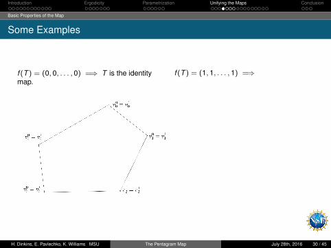
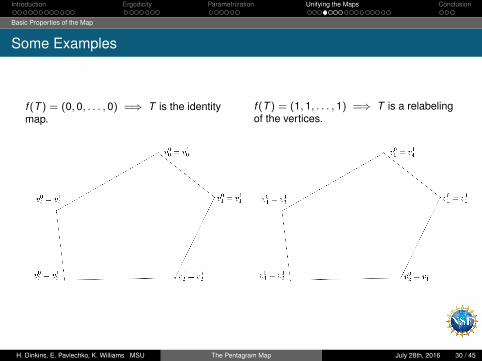
Some Examples
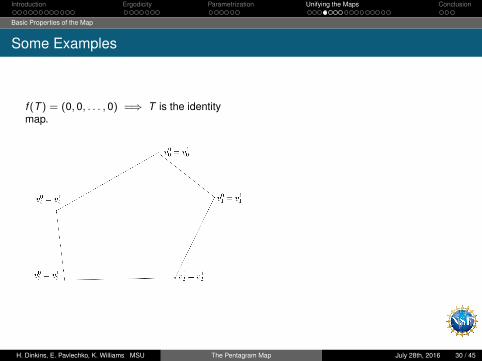
f (T ) = (0, 0, . . . , 0) =⇒
T is the identitymap.
f (T ) = (1, 1, . . . , 1) =⇒ T is a relabelingof the vertices.
H. Dinkins, E. Pavlechko, K. Williams MSU The Pentagram Map July 28th, 2016 30 / 45
Introduction Ergodicity Parametrization Unifying the Maps Conclusion
Basic Properties of the Map
Some Examples
f (T ) = (0, 0, . . . , 0) =⇒ T is the identitymap.
f (T ) = (1, 1, . . . , 1) =⇒
T is a relabelingof the vertices.
H. Dinkins, E. Pavlechko, K. Williams MSU The Pentagram Map July 28th, 2016 30 / 45
Introduction Ergodicity Parametrization Unifying the Maps Conclusion
Basic Properties of the Map
Some Examples
f (T ) = (0, 0, . . . , 0) =⇒ T is the identitymap.
f (T ) = (1, 1, . . . , 1) =⇒ T is a relabelingof the vertices.
H. Dinkins, E. Pavlechko, K. Williams MSU The Pentagram Map July 28th, 2016 30 / 45

Introduction Ergodicity Parametrization Unifying the Maps Conclusion
Basic Properties of the Map
Some Examples
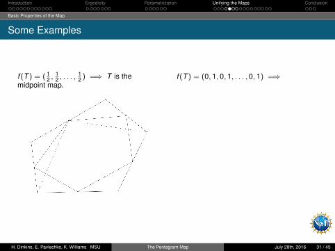
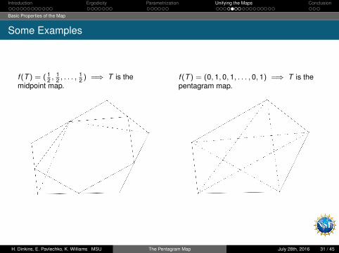
f (T ) = ( 12 ,
12 , . . . ,
12 ) =⇒
T is themidpoint map.
f (T ) = (0, 1, 0, 1, . . . , 0, 1) =⇒ T is thepentagram map.
H. Dinkins, E. Pavlechko, K. Williams MSU The Pentagram Map July 28th, 2016 31 / 45

Introduction Ergodicity Parametrization Unifying the Maps Conclusion
Basic Properties of the Map
Some Examples
f (T ) = ( 12 ,
12 , . . . ,
12 ) =⇒ T is the
midpoint map.
f (T ) = (0, 1, 0, 1, . . . , 0, 1) =⇒ T is thepentagram map.
H. Dinkins, E. Pavlechko, K. Williams MSU The Pentagram Map July 28th, 2016 31 / 45
Introduction Ergodicity Parametrization Unifying the Maps Conclusion
Basic Properties of the Map
Some Examples
f (T ) = ( 12 ,
12 , . . . ,
12 ) =⇒ T is the
midpoint map.f (T ) = (0, 1, 0, 1, . . . , 0, 1) =⇒
T is thepentagram map.
H. Dinkins, E. Pavlechko, K. Williams MSU The Pentagram Map July 28th, 2016 31 / 45
Introduction Ergodicity Parametrization Unifying the Maps Conclusion
Basic Properties of the Map
Some Examples
f (T ) = ( 12 ,
12 , . . . ,
12 ) =⇒ T is the
midpoint map.f (T ) = (0, 1, 0, 1, . . . , 0, 1) =⇒ T is thepentagram map.
H. Dinkins, E. Pavlechko, K. Williams MSU The Pentagram Map July 28th, 2016 31 / 45
Introduction Ergodicity Parametrization Unifying the Maps Conclusion
Basic Properties of the Map
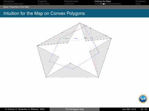
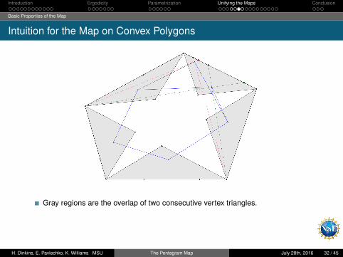
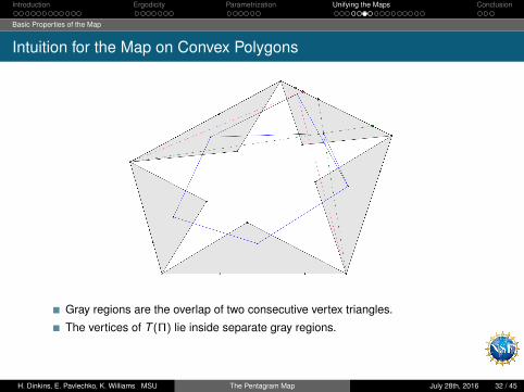
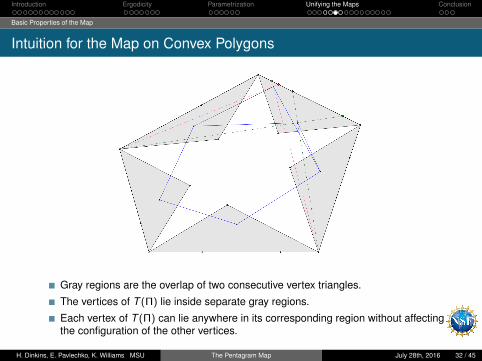
Intuition for the Map on Convex Polygons
Gray regions are the overlap of two consecutive vertex triangles.
The vertices of T (Π) lie inside separate gray regions.
Each vertex of T (Π) can lie anywhere in its corresponding region without affectingthe configuration of the other vertices.
H. Dinkins, E. Pavlechko, K. Williams MSU The Pentagram Map July 28th, 2016 32 / 45
Introduction Ergodicity Parametrization Unifying the Maps Conclusion
Basic Properties of the Map
Convexity and the GPM
All the maps we’ve looked at previously preserve convexity.
Do all GPMs preserve convexity ?Unfortunately, no.
H. Dinkins, E. Pavlechko, K. Williams MSU The Pentagram Map July 28th, 2016 33 / 45
Introduction Ergodicity Parametrization Unifying the Maps Conclusion
Basic Properties of the Map
Convexity and the GPM
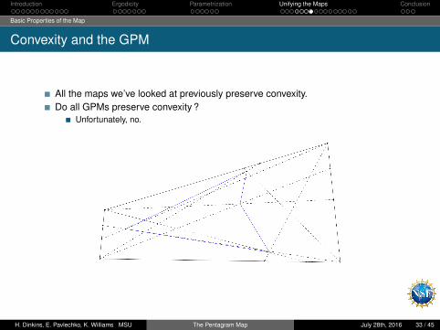
All the maps we’ve looked at previously preserve convexity.Do all GPMs preserve convexity ?
Unfortunately, no.
H. Dinkins, E. Pavlechko, K. Williams MSU The Pentagram Map July 28th, 2016 33 / 45
Introduction Ergodicity Parametrization Unifying the Maps Conclusion
Basic Properties of the Map
Convexity and the GPM
All the maps we’ve looked at previously preserve convexity.Do all GPMs preserve convexity ?
Unfortunately, no.
H. Dinkins, E. Pavlechko, K. Williams MSU The Pentagram Map July 28th, 2016 33 / 45
Introduction Ergodicity Parametrization Unifying the Maps Conclusion
Regular Polygon Case
A Special Type of GPM
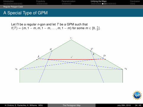
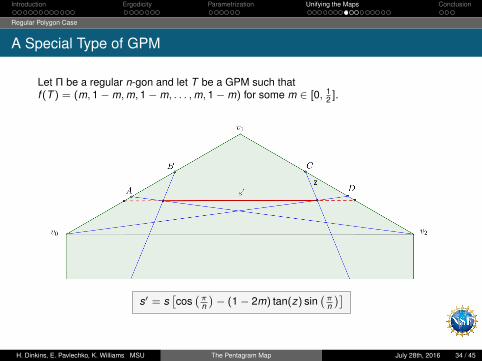
Let Π be a regular n-gon and let T be a GPM such thatf (T ) = (m, 1−m,m, 1−m, . . . ,m, 1−m) for some m ∈ [0, 1
2 ].
s′ = s[cos
(πn
)− (1− 2m) tan(z) sin
(πn
)]
H. Dinkins, E. Pavlechko, K. Williams MSU The Pentagram Map July 28th, 2016 34 / 45
Introduction Ergodicity Parametrization Unifying the Maps Conclusion
Regular Polygon Case
A Special Type of GPM
Let Π be a regular n-gon and let T be a GPM such thatf (T ) = (m, 1−m,m, 1−m, . . . ,m, 1−m) for some m ∈ [0, 1
2 ].
s′ = s[cos
(πn
)− (1− 2m) tan(z) sin
(πn
)]
H. Dinkins, E. Pavlechko, K. Williams MSU The Pentagram Map July 28th, 2016 34 / 45
Introduction Ergodicity Parametrization Unifying the Maps Conclusion
Regular Polygon Case
A Special Type of GPM
Found using :
Multiple Law of Sines applications
Similar triangles
Symmetry of the regular polygon
P(T k+1(Π))
P(T k (Π))= cos
(πn
)− (1− 2m) sin
(πn
)tan(z)
Plugging in m = 0 reduces this equation to P(T k+1(Π))
P(T k (Π))=
cos( 2πn )
cos( πn )
which is what
we obtained previously.
So T is a convexity preserving GPM on regular polygons and T k (Π) converges toa point.
H. Dinkins, E. Pavlechko, K. Williams MSU The Pentagram Map July 28th, 2016 35 / 45
Introduction Ergodicity Parametrization Unifying the Maps Conclusion
Regular Polygon Case
A Special Type of GPM
What makes this map important ?
It is a nontrivial convexity-preserving GPM on regular polygons.
This very "normal" type of GPM preserves regularity and decreases side length ina predictable way.
H. Dinkins, E. Pavlechko, K. Williams MSU The Pentagram Map July 28th, 2016 36 / 45
Introduction Ergodicity Parametrization Unifying the Maps Conclusion
General Polygons
GPM Properties
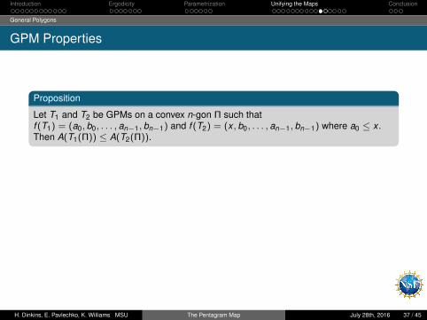
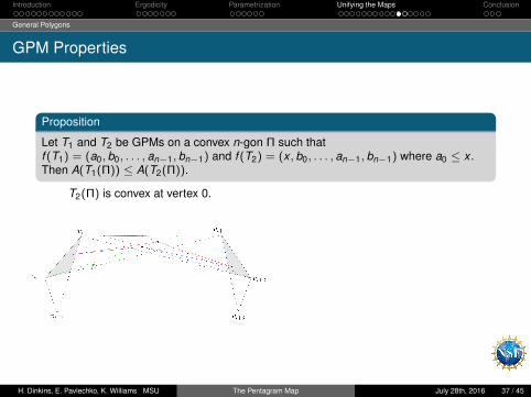
Proposition
Let T1 and T2 be GPMs on a convex n-gon Π such thatf (T1) = (a0, b0, . . . , an−1, bn−1) and f (T2) = (x , b0, . . . , an−1, bn−1) where a0 ≤ x .Then A(T1(Π)) ≤ A(T2(Π)).
T2(Π) is convex at vertex 0. T2(Π) is not convex at vertex 0
H. Dinkins, E. Pavlechko, K. Williams MSU The Pentagram Map July 28th, 2016 37 / 45
Introduction Ergodicity Parametrization Unifying the Maps Conclusion
General Polygons
GPM Properties
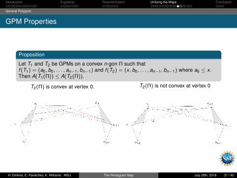
Proposition
Let T1 and T2 be GPMs on a convex n-gon Π such thatf (T1) = (a0, b0, . . . , an−1, bn−1) and f (T2) = (x , b0, . . . , an−1, bn−1) where a0 ≤ x .Then A(T1(Π)) ≤ A(T2(Π)).
T2(Π) is convex at vertex 0.
T2(Π) is not convex at vertex 0
H. Dinkins, E. Pavlechko, K. Williams MSU The Pentagram Map July 28th, 2016 37 / 45
Introduction Ergodicity Parametrization Unifying the Maps Conclusion
General Polygons
GPM Properties
Proposition
Let T1 and T2 be GPMs on a convex n-gon Π such thatf (T1) = (a0, b0, . . . , an−1, bn−1) and f (T2) = (x , b0, . . . , an−1, bn−1) where a0 ≤ x .Then A(T1(Π)) ≤ A(T2(Π)).
T2(Π) is convex at vertex 0. T2(Π) is not convex at vertex 0
H. Dinkins, E. Pavlechko, K. Williams MSU The Pentagram Map July 28th, 2016 37 / 45
Introduction Ergodicity Parametrization Unifying the Maps Conclusion
General Polygons
GPM Properties
Corollary
Let TP be the pentagram map and T be any other GPM on a convex polygon Π. ThenA(TP(Π)) < A(T (Π)).
The process seen in the previous proposition terminates with the pentagram map.
Recall that last time we provedA(T k+1
P (Π))
A(T kP (Π))
< 1415 where Π is a pentagon.
We can use this corollary to obtain a better bound on the rate of area reduction forthe pentagram map on pentagons.
H. Dinkins, E. Pavlechko, K. Williams MSU The Pentagram Map July 28th, 2016 38 / 45
Introduction Ergodicity Parametrization Unifying the Maps Conclusion
The Pentagon Case
A Better Bound
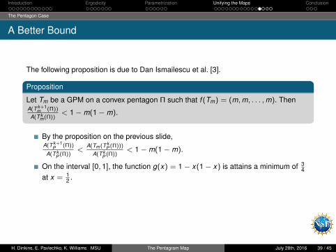
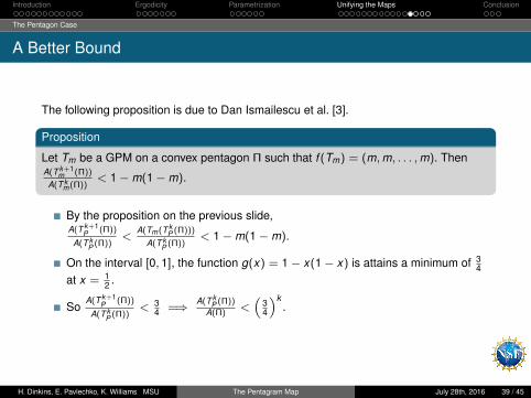
The following proposition is due to Dan Ismailescu et al. [3].
Proposition
Let Tm be a GPM on a convex pentagon Π such that f (Tm) = (m,m, . . . ,m). ThenA(T k+1
m (Π))
A(T km(Π))
< 1−m(1−m).
By the proposition on the previous slide,A(T k+1
P (Π))
A(T kP (Π))
<A(Tm(T k
P (Π)))
A(T kP (Π))
< 1−m(1−m).
On the interval [0, 1], the function g(x) = 1− x(1− x) is attains a minimum of 34
at x = 12 .
SoA(T k+1
P (Π))
A(T kP (Π))
< 34 =⇒ A(T k
P (Π))
A(Π)<(
34
)k.
H. Dinkins, E. Pavlechko, K. Williams MSU The Pentagram Map July 28th, 2016 39 / 45
Introduction Ergodicity Parametrization Unifying the Maps Conclusion
The Pentagon Case
A Better Bound
The following proposition is due to Dan Ismailescu et al. [3].
Proposition
Let Tm be a GPM on a convex pentagon Π such that f (Tm) = (m,m, . . . ,m). ThenA(T k+1
m (Π))
A(T km(Π))
< 1−m(1−m).
By the proposition on the previous slide,A(T k+1
P (Π))
A(T kP (Π))
<A(Tm(T k
P (Π)))
A(T kP (Π))
< 1−m(1−m).
On the interval [0, 1], the function g(x) = 1− x(1− x) is attains a minimum of 34
at x = 12 .
SoA(T k+1
P (Π))
A(T kP (Π))
< 34 =⇒ A(T k
P (Π))
A(Π)<(
34
)k.
H. Dinkins, E. Pavlechko, K. Williams MSU The Pentagram Map July 28th, 2016 39 / 45
Introduction Ergodicity Parametrization Unifying the Maps Conclusion
The Pentagon Case
A More General Result
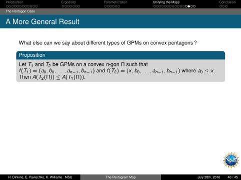
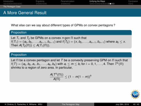
What else can we say about different types of GPMs on convex pentagons ?
Proposition
Let T1 and T2 be GPMs on a convex n-gon Π such thatf (T1) = (a0, b0, . . . , an−1, bn−1) and f (T2) = (x , b0, . . . , an−1, bn−1) where a0 ≤ x .Then A(T2(Π)) ≤ A(T1(Π)).
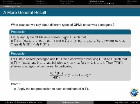
Proposition
Let Π be a convex pentagon and let T be a convexity preserving GPM on Π such thatf (T ) = (a0, b0, a1, b1, . . . , a4, b4) with ai ≤ m ≤ bi for i = 0, 1, . . . , 4. Then T k (Π)shrinks to a region of zero area. In particular,
A(T k (Π))
A(Π)≤ (1−m(1−m))k
Proof :
Apply the top proposition to each coordinate of f (T ).
H. Dinkins, E. Pavlechko, K. Williams MSU The Pentagram Map July 28th, 2016 40 / 45
Introduction Ergodicity Parametrization Unifying the Maps Conclusion
The Pentagon Case
A More General Result
What else can we say about different types of GPMs on convex pentagons ?
Proposition
Let T1 and T2 be GPMs on a convex n-gon Π such thatf (T1) = (a0, b0, . . . , an−1, bn−1) and f (T2) = (x , b0, . . . , an−1, bn−1) where a0 ≤ x .Then A(T2(Π)) ≤ A(T1(Π)).
Proposition
Let Π be a convex pentagon and let T be a convexity preserving GPM on Π such thatf (T ) = (a0, b0, a1, b1, . . . , a4, b4) with ai ≤ m ≤ bi for i = 0, 1, . . . , 4. Then T k (Π)shrinks to a region of zero area. In particular,
A(T k (Π))
A(Π)≤ (1−m(1−m))k
Proof :
Apply the top proposition to each coordinate of f (T ).
H. Dinkins, E. Pavlechko, K. Williams MSU The Pentagram Map July 28th, 2016 40 / 45
Introduction Ergodicity Parametrization Unifying the Maps Conclusion
The Pentagon Case
Review of GPM Results
We proved convergence to a point for a special type of GPM applied to regularpolygons.
We obtained a better bound of the rate of area decrease for the pentagram map.
We proved that a restricted class of GPMs applied to a convex pentagon shrinksto a region of zero area. Furthermore, we provided a bound on the rate of areadecrease.
H. Dinkins, E. Pavlechko, K. Williams MSU The Pentagram Map July 28th, 2016 41 / 45
Introduction Ergodicity Parametrization Unifying the Maps Conclusion
The Pentagon Case
Future GPM Directions
Given a polygon Π, find a sufficient condition for a GPM to be aconvexity-preserving map on Π.
Investigate different types of GPMs.
Study GPMs on polygons with n > 5 vertices.
H. Dinkins, E. Pavlechko, K. Williams MSU The Pentagram Map July 28th, 2016 42 / 45
Introduction Ergodicity Parametrization Unifying the Maps Conclusion
Overall Results
Generalized the iteration procedure.
Improved the rate of convergence for Area to 34 .
Made a program to assist in computation of the pentagram map.
Set up methods for simpler geometric proofs for convergence.
Worked with matrices to represent convergence.
Built upon previously established results by Richard Schwartz.
Proved convergence to a point for a restricted class of pentagons.
H. Dinkins, E. Pavlechko, K. Williams MSU The Pentagram Map July 28th, 2016 43 / 45

Introduction Ergodicity Parametrization Unifying the Maps Conclusion
THANK YOU
Dr. Sun
Professor Vollmar for his Pythonexpertise
Missouri State University for hostingus
The NSF : Grant #1559911
H. Dinkins, E. Pavlechko, K. Williams MSU The Pentagram Map July 28th, 2016 44 / 45
Introduction Ergodicity Parametrization Unifying the Maps Conclusion
References
Erik Hintikka and Xingping Sun.Convergence of sequences of polygons.Involve, 2016.
Ilse Ipsen and Teresa Selee.Ergodicity coefficients defined by vector norms.Society for Industrial and Applied Mathematics, 32(1) :153 – 200, 2011.
Dan Ismailescu et al.Area problems involving kasner polygons.ArXhiv : 0910.0452v1, 2009.
Richard Schwartz.The pentagram map.Experimental Mathematics, 51 :71–81, 1994.
H. Dinkins, E. Pavlechko, K. Williams MSU The Pentagram Map July 28th, 2016 45 / 45