Embed Size (px)
Citation preview
Dynamics of Quantum Many-BodySystems from
Monte Carlo simulations
Francesco Pederiva
I.N.F.N. and Physics Department, University of Trento - ITALY
INT - Seattle - October 24, 2012

Dynamics ofQuantum
Many-BodySystems fromMonte Carlosimulations
FrancescoPederiva
QMC andResponseFunctions
DynamicResponseFunction
Ill posedproblems
Integralkernels
Condensed4He
Conclusions
Collaborators
Alessandro Roggero (Trento)
Giuseppina Orlandini (Trento)
Dynamics ofQuantum
Many-BodySystems fromMonte Carlosimulations
FrancescoPederiva
QMC andResponseFunctions
DynamicResponseFunction
Ill posedproblems
Integralkernels
Condensed4He
Conclusions
Outline
QMC and Response Functions
Dynamic Response Functions:Integral transform methodsIll-Posed problemsRegularization techniques
Integral Kernels for Quantum Monte CarloLaplace Kernel and imaginary-time correlationsA better Kernel
ResultsSuperfluid He4

Dynamics ofQuantum
Many-BodySystems fromMonte Carlosimulations
FrancescoPederiva
QMC andResponseFunctions
DynamicResponseFunction
Ill posedproblems
Integralkernels
Condensed4He
Conclusions
QMC and Response functionsA few canonical statements.
Projection QMC methods are acknowledged to give useful andaccurate estimates of expectations on the ground state of agiven Hamiltonian H.
Start from a ”trial wavefunction” that can be expanded alongthe basis of eigenstates of H, applying an imaginary timepropagator formally projects the ground state out of the initialstate. This is completely general, and does not depend on therepresentation used (configuration space, momentum space,Fock space, ...).
lim⌧→∞ e− ⌧�h (H−E0)� T � = lim
⌧→∞�n e− ⌧�h (En−E0)��n���n� T � == ��0� T ���0�

Dynamics ofQuantum
Many-BodySystems fromMonte Carlosimulations
FrancescoPederiva
QMC andResponseFunctions
DynamicResponseFunction
Ill posedproblems
Integralkernels
Condensed4He
Conclusions
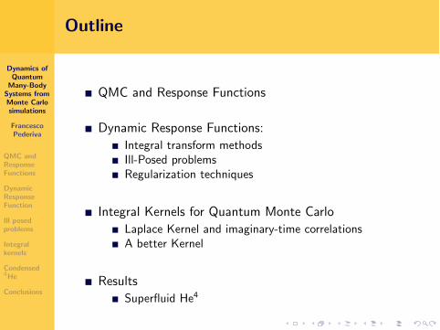
QMC and Response functionsA few canonical statements.
It is clear from the previous analysis of imaginary timepropagation that the information about excited states must beburied into the filtering process.
How do we extract it?
The good, old answer is with an inverse Laplace transform!(See e.g. L-QCD calculations, David Ceperley et al., theANL/LANL group....). However, everebody knows that this isan ill posed problem.
Here we want to analyize the problem a little more closely.
Dynamics ofQuantum
Many-BodySystems fromMonte Carlosimulations
FrancescoPederiva
QMC andResponseFunctions
DynamicResponseFunction
Ill posedproblems
Integralkernels
Condensed4He
Conclusions
QMC and Response functionsA few canonical statements.
It is clear from the previous analysis of imaginary timepropagation that the information about excited states must beburied into the filtering process.
How do we extract it?
The good, old answer is with an inverse Laplace transform!(See e.g. L-QCD calculations, David Ceperley et al., theANL/LANL group....). However, everebody knows that this isan ill posed problem.
Here we want to analyize the problem a little more closely.

Dynamics ofQuantum
Many-BodySystems fromMonte Carlosimulations
FrancescoPederiva
QMC andResponseFunctions
DynamicResponseFunction
Ill posedproblems
Integralkernels
Condensed4He
Conclusions
Dynamic Response Function
Spectral representation of DRF
R(!) =�⌫�� ⌫ �O � 0��2� [! − (E⌫ − E0)]
=�⌫� 0�O†� ⌫�� ⌫ �O � 0�� (! − (E⌫ − E0))
= � 0�O†�⌫� ⌫�� ⌫ �� [! − (E⌫ − E0)] O � 0�
= � 0�O†� �! − (H − E0)� O � 0�� ⌫� �→ complete set of Hamiltonian eigenstates
O �→ excitation operator
! �→ energy transfer (�h = 1)
Dynamics ofQuantum
Many-BodySystems fromMonte Carlosimulations
FrancescoPederiva
QMC andResponseFunctions
DynamicResponseFunction
Ill posedproblems
Integralkernels
Condensed4He
Conclusions
Integral Transform Methods
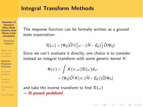
The response function can be formally written as a groundstate expectation:
R(!) = � 0�O†� �! − (H − E0)� O � 0�Since we can’t evaluate it directly, one choice is to considerinstead an integral transform with some generic kernel K :
�(�) = � K(�,!)R(!)d!
= � 0�O†K(�, (H − E0))O � 0�and take the inverse transform to find R(!)→ ill-posed problem!.

Dynamics ofQuantum
Many-BodySystems fromMonte Carlosimulations
FrancescoPederiva
QMC andResponseFunctions
DynamicResponseFunction
Ill posedproblems
Integralkernels
Condensed4He
Conclusions
Integral Transform methods
Some ”obvious” characteristics of a good kernel should be:
the transform �(�) is easy to calculate
the inversion of the transform can be made stable
K(�,!) is approximately �(� − !) (in principle not strictlynecessary)

Dynamics ofQuantum
Many-BodySystems fromMonte Carlosimulations
FrancescoPederiva
QMC andResponseFunctions
DynamicResponseFunction
Ill posedproblems
Integralkernels
Condensed4He
Conclusions
Integral transforms and Ill-posed problems
Ill-Posed Problems [Hadamard]
A problem is called ill-posed when one of the following occours
the solution does not exist or it is not unique
the solution does not depend continuosly on the data
An intuitive way to see the problem is to considerfn(y) = sin(ny)
g(x) = � b
aK(x , y) fn(y)dy
n→∞���→ 0
the integration process has a smoothening e↵ect.
Dynamics ofQuantum
Many-BodySystems fromMonte Carlosimulations
FrancescoPederiva
QMC andResponseFunctions
DynamicResponseFunction
Ill posedproblems
Integralkernels
Condensed4He
Conclusions
Integral transforms and Ill-posed problems
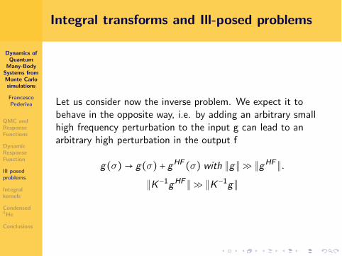
Let us consider now the inverse problem. We expect it tobehave in the opposite way, i.e. by adding an arbitrary smallhigh frequency perturbation to the input g can lead to anarbitrary high perturbation in the output f
g(�)→ g(�) + gHF (�) with �g�� �gHF �.�K−1gHF �� �K−1g�

Dynamics ofQuantum
Many-BodySystems fromMonte Carlosimulations
FrancescoPederiva
QMC andResponseFunctions
DynamicResponseFunction
Ill posedproblems
Integralkernels
Condensed4He
Conclusions
Singular Value Decomposition (SVD)
We can make a discretization of the Integral transform
g(x) = � b
aK(x , y)f (y)dy �→ gi = N�
k
↵kKik fk i ∈ [1,N]gi ≡ g(xi) Kik ≡ K(xi , yk) fk ≡ f (yk)
The SVD of the matrix K is a factorization of the form
K = U⌃V T with U,V ,⌃ ∈ NxN
with U,V orthogonal and ⌃ = diag[�1, . . . ,�N].The columns uj of U and vj of V can be regarded asorthonormal basis vectors of N and the following holds
Kvj = �j uj KT uj = �j vj

Dynamics ofQuantum
Many-BodySystems fromMonte Carlosimulations
FrancescoPederiva
QMC andResponseFunctions
DynamicResponseFunction
Ill posedproblems
Integralkernels
Condensed4He
Conclusions
Singular Value Decomposition (SVD) II
In terms of the SVD of the matrix K the direct and inverseproblems can be rewritten as
g = Kf = N�j
�j(vTj f )uj f = K−1g = N�
j
uTj g
�jvj
If the matrix K is the result of discretization of a FredholmIntegral equation of the 1st kind the following basic propertiesholds
the singular values �i decay fast towards zero
the singular vectors ui ,vi have increasing frequencies
We can use the decay rate of singular values to define a sort ofdegree of ill − posedness

Dynamics ofQuantum
Many-BodySystems fromMonte Carlosimulations
FrancescoPederiva
QMC andResponseFunctions
DynamicResponseFunction
Ill posedproblems
Integralkernels
Condensed4He
Conclusions
Singular Value Spectrum

Dynamics ofQuantum
Many-BodySystems fromMonte Carlosimulations
FrancescoPederiva
QMC andResponseFunctions
DynamicResponseFunction
Ill posedproblems
Integralkernels
Condensed4He
Conclusions
Regularization techniques
As an escape, it is possible to approximate the original ill-posedproblem with a well-posed one, constraining the solution withknown features (eg. smoothness, sign, asymptotic behavior...)in this way, (i.e. changing the problem...), the solution iswell-defined
In most approaches we have minimization problems of the form
minf
D �Kf , g� + ↵L �f �where
D is a likelihood function (eg. Chi-squared, euclideannorm)
L is a penalty functional that enforces eg. smoothness
↵ is the regularization parameter

Dynamics ofQuantum
Many-BodySystems fromMonte Carlosimulations
FrancescoPederiva
QMC andResponseFunctions
DynamicResponseFunction
Ill posedproblems
Integralkernels
Condensed4He
Conclusions
Integral kernels - Laplace
Projection QMC methods exploit the long time behavior of theimaginary-time propagator
e−⌧ H ��0� = ∞�n=0 e−⌧En� n��0�� n� ⌧→∞���→ e−⌧E0� 0��0�� 0�
In this framework it is natural to consider the Laplace kernel:
K(�,!) = e−�!
The transform becomes an imaginary-time correlation function:
�(�) = � 0�O†e−�HO � 0�� 0� 0� = � 0�O†(0)O(�)� 0�� 0� 0� .

Dynamics ofQuantum
Many-BodySystems fromMonte Carlosimulations
FrancescoPederiva
QMC andResponseFunctions
DynamicResponseFunction
Ill posedproblems
Integralkernels
Condensed4He
Conclusions
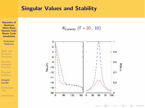
Singular Values and Stability
In order to understand how bad the Laplace kernel really is. letus compare its SVD spectrum with that of a Lorentz kernel,known to be more stable for inversion.
Laplace kernel [QMC methods]
KLaplace(�,!) = e−�!
Lorentz kernel [LIT method]
KLorentz(�,!) = �
�2 + (� − !)2where the parameter � controls the width of the kernel.

Dynamics ofQuantum
Many-BodySystems fromMonte Carlosimulations
FrancescoPederiva
QMC andResponseFunctions
DynamicResponseFunction
Ill posedproblems
Integralkernels
Condensed4He
Conclusions
Singular Values and Stability
KLorentz {� = 20}
Dynamics ofQuantum
Many-BodySystems fromMonte Carlosimulations
FrancescoPederiva
QMC andResponseFunctions
DynamicResponseFunction
Ill posedproblems
Integralkernels
Condensed4He
Conclusions
Singular Values and Stability
KLorentz {� = 20 , 10}

Dynamics ofQuantum
Many-BodySystems fromMonte Carlosimulations
FrancescoPederiva
QMC andResponseFunctions
DynamicResponseFunction
Ill posedproblems
Integralkernels
Condensed4He
Conclusions
Singular Values and Stability
KLorentz {� = 20 , 10 , 5}

Dynamics ofQuantum
Many-BodySystems fromMonte Carlosimulations
FrancescoPederiva
QMC andResponseFunctions
DynamicResponseFunction
Ill posedproblems
Integralkernels
Condensed4He
Conclusions
Singular Values and Stability
KLorentz {� = 20 , 10 , 5} KLaplace

Dynamics ofQuantum
Many-BodySystems fromMonte Carlosimulations
FrancescoPederiva
QMC andResponseFunctions
DynamicResponseFunction
Ill posedproblems
Integralkernels
Condensed4He
Conclusions
Integral Kernels - Laplace-like
We now want to build an integral kernel which can becalculated in QMC methods and that has a shape closer to theLorentz kernel. In general, a better approximation of a Dirac �function (which has obviously a flat spectrum) seems to be abetter guess for the kernel.
This is an ”obvious” statement, but it can be madequantitative by means of the SVD analysis!

Dynamics ofQuantum
Many-BodySystems fromMonte Carlosimulations
FrancescoPederiva
QMC andResponseFunctions
DynamicResponseFunction
Ill posedproblems
Integralkernels
Condensed4He
Conclusions
Singular Values and Stability
Let us consider the following kernel, that we can easily see asbuilt out of Laplace kernels with di↵erent imaginary times(Sumudu Transform):
K(�,!,N) = 1
��2−!
� − 2−2!� �N = N�
k=0�N
k�(−1)ke− ln(2)(N+k)!
�
(1)As N →∞ the kernel width becomes smaller.

Dynamics ofQuantum
Many-BodySystems fromMonte Carlosimulations
FrancescoPederiva
QMC andResponseFunctions
DynamicResponseFunction
Ill posedproblems
Integralkernels
Condensed4He
Conclusions
Integral Kernels - New Kernel (SV spectrum)

Dynamics ofQuantum
Many-BodySystems fromMonte Carlosimulations
FrancescoPederiva
QMC andResponseFunctions
DynamicResponseFunction
Ill posedproblems
Integralkernels
Condensed4He
Conclusions
Path Integral Methods
How do we calculate imaginary-time correlation function?
Path Integral based methods (VPI,PIGS,RQMC) have access topure estimators and are naturally suited for imaginary-timeproperties since we simulate already full imaginary-time paths.
Consider an imaginary-time path of length 2⌧ + � as our”walker” and discretize the path in M time-slices of size�⌧ = (2⌧ + �)�M, then:
CO(�) = � T �e−⌧(H−E0)O†e−�(H−E0)Oe−⌧(H−E0)� T �� T �e−(2⌧+�)(H−E0)� T �
⌧→∞���→ � 0�O†e−�(H−E0)O � 0�� 0� 0� = � 0�O†(0)O(�)� 0�� 0� 0�
Dynamics ofQuantum
Many-BodySystems fromMonte Carlosimulations
FrancescoPederiva
QMC andResponseFunctions
DynamicResponseFunction
Ill posedproblems
Integralkernels
Condensed4He
Conclusions
Condensed 4He
Liquid 4He is the ”simplest” many-body system on which wecan test our kernels.Quick reminders:
Liquid 4He becomes superfluid at temperatures < 2.172K
The interaction is essentially Van der Waals. At saturationthe binding energy per atom is 7.12K (1K =8.2×10⁻¹¹MeV)

Dynamics ofQuantum
Many-BodySystems fromMonte Carlosimulations
FrancescoPederiva
QMC andResponseFunctions
DynamicResponseFunction
Ill posedproblems
Integralkernels
Condensed4He
Conclusions
Density response of superfluid He4
The density response is usually measured by means of neutronscattering.
http://www.cm.ph.bham.ac.uk/group/whoswho/blackburn/blackburn.html

Dynamics ofQuantum
Many-BodySystems fromMonte Carlosimulations
FrancescoPederiva
QMC andResponseFunctions
DynamicResponseFunction
Ill posedproblems
Integralkernels
Condensed4He
Conclusions
Density response of superfluid He4
QMC calculation
64 He4 atoms in a cubic box with Periodic BoundaryConditions
realistic e↵ective interaction: HFDHE2 pair-potential[Aziz (1979)]. Notice that in condensed 4He 3-body forceswould be needed.
Trial-function with two and three-body correlations
Reptation Quantum Monte Carlo (RQMC) [Baroni (1999)]
Dynamics ofQuantum
Many-BodySystems fromMonte Carlosimulations
FrancescoPederiva
QMC andResponseFunctions
DynamicResponseFunction
Ill posedproblems
Integralkernels
Condensed4He
Conclusions
Density response of superfluid He4
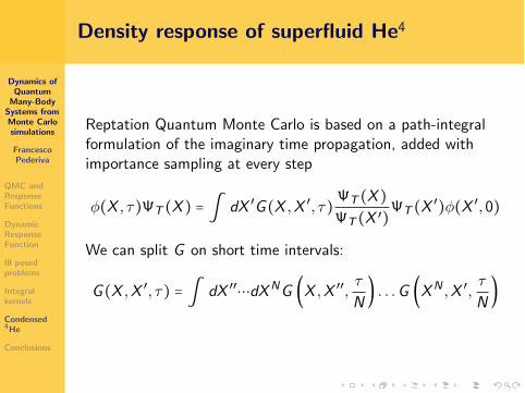
Reptation Quantum Monte Carlo is based on a path-integralformulation of the imaginary time propagation, added withimportance sampling at every step
�(X , ⌧) T (X) = � dX ′G(X ,X ′, ⌧) T (X) T (X ′) T (X ′)�(X ′,0)
We can split G on short time intervals:
G(X ,X ′, ⌧) = � dX ′′�dXNG �X ,X ′′, ⌧
N� . . .G �XN ,X ′, ⌧
N�

Dynamics ofQuantum
Many-BodySystems fromMonte Carlosimulations
FrancescoPederiva
QMC andResponseFunctions
DynamicResponseFunction
Ill posedproblems
Integralkernels
Condensed4He
Conclusions
Density response of superfluid He4
The splitted Green’s function can be in turn be redefined as aproduct of importance sampled Green’s functions:
G(X ,X ′, ⌧) ≡ G(X .X ′, ⌧) T (X) T (X ′) =
= � dX ′′�dXN G �X ,X ′′, ⌧
N� . . . G �XN ,X ′, ⌧
N�
In the short time approximation, at order �⌧ = ⌧�N(Trotter):
G(X ,X ′,�⌧) ∼ e−�X−∇ T (X ′)
T (X ′) −X′�2
2D�⌧ e− 1
2�H T (X) T (X ′) +H T (X ′)
T (X) ��⌧

Dynamics ofQuantum
Many-BodySystems fromMonte Carlosimulations
FrancescoPederiva
QMC andResponseFunctions
DynamicResponseFunction
Ill posedproblems
Integralkernels
Condensed4He
Conclusions
Density response of superfluid 4He
We are therefore lead to sample a reptile, i.e. a path {X0�XN}in which each time slice is sampled evolving the previous onewith a Langevin dynamics:
Xi+1 = Xi +�⌧H T (Xi) T (Xi) + ⌘(Xi ,Xi + 1,�⌧)
The reptiles are sampled by randomly choosing one of the twoends, sampling a further point of the path, and destroyng thelast point on the oppsite site.In the middle of the path the points are propagated of animaginary time ⌧�2.

Dynamics ofQuantum
Many-BodySystems fromMonte Carlosimulations
FrancescoPederiva
QMC andResponseFunctions
DynamicResponseFunction
Ill posedproblems
Integralkernels
Condensed4He
Conclusions
ESTIMATORS
Energy:
E = 1
2[Eloc(0) + Eloc(⌧)] where Eloc = H T (X)
T (X)Other (local):
�O� = 1
⌧ − 2��� ⌧−�
�O(⌧ ′)d⌧ ′�
� should be large enough to avoid bias from the trial function.The operator averaged at times 0 and ⌧ gives the mixedestimate � 0�O � T � usually computed in DMC.

Dynamics ofQuantum
Many-BodySystems fromMonte Carlosimulations
FrancescoPederiva
QMC andResponseFunctions
DynamicResponseFunction
Ill posedproblems
Integralkernels
Condensed4He
Conclusions
An interesting feature of RQMC is the fact that expectationscomputed at the center of the sample ”reptile” are no longerdependent on the importance function.
from A. Roggero M.Sc. thesis

Dynamics ofQuantum
Many-BodySystems fromMonte Carlosimulations
FrancescoPederiva
QMC andResponseFunctions
DynamicResponseFunction
Ill posedproblems
Integralkernels
Condensed4He
Conclusions
Density response of superfluid 4He
We are interested in the density response of the system, in thiscase the Response function is the so-called Dynamic StructureFactor
S(q,!) = 1
N�⌫�� ⌫ �⇢q � 0��2� (! − (E⌫ − E0))
where ⇢q is the Fourier Transform of the density operator:⇢q ≡ ∑j e
iqrk .
Dynamics ofQuantum
Many-BodySystems fromMonte Carlosimulations
FrancescoPederiva
QMC andResponseFunctions
DynamicResponseFunction
Ill posedproblems
Integralkernels
Condensed4He
Conclusions
Density response of superfluid 4He
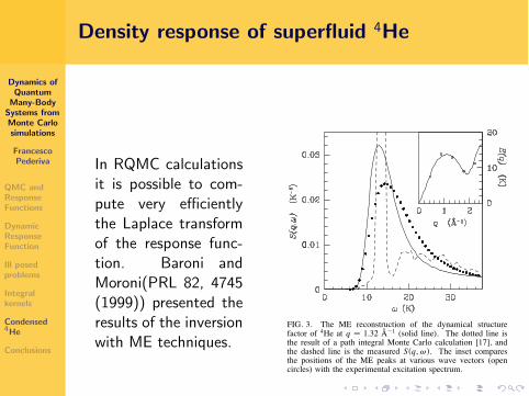
In RQMC calculationsit is possible to com-pute very e�cientlythe Laplace transformof the response func-tion. Baroni andMoroni(PRL 82, 4745(1999)) presented theresults of the inversionwith ME techniques.
VOLUME 82, NUMBER 24 P HY S I CA L REV I EW LE T T ER S 14 JUNE 1999
FIG. 3. The ME reconstruction of the dynamical structurefactor of 4He at q ≠ 1.32 Å21 (solid line). The dotted line isthe result of a path integral Monte Carlo calculation [17], andthe dashed line is the measured Ssq, vd. The inset comparesthe positions of the ME peaks at various wave vectors (opencircles) with the experimental excitation spectrum.
f-sum rule, ≠Fsq, tdy≠tjt≠0
≠ q2, is also fulfilled withhigh precision.Inferring the dynamical structure factor Ssq, vd
requires an inverse Laplace transform, Fsq, td ≠R`0
Ssq, vdexps2vtd dv. We perform a maximum en-tropy (ME) analysis [16] of our data, with results similarto those obtained in Ref. [17]. The ME reconstructionof Ssq, vd, shown in Fig. 3, is too smooth and does notreproduce the sharp features exhibited by the experimen-tal structure factor in the superfluid phase. Some knownproperties of the spectrum are recovered: The presence ofa gap in the excitation spectrum is clearly revealed, andthe position of the peak of the reconstructed dynamicalresponse closely follows the measured dispersion of theelementary excitations [4,17]. However, the generalreliability of the ME analysis as a predictive tool, withthe statistical accuracy of the data typically achieved fromthe simulation of continuum systems, is hard to assess.We finally outline the calculation of the superfluid den-
sity rs. The superfluid transition is of interest even atzero temperature, for instance, in the presence of an exter-nal disordered potential V
ext
. We can compute rs fromthe diffusion coefficient of the center of mass motion,rsyr ≠ limt!` Dstd, which is the zero temperature limitof the winding number estimator used in path integralsimulations [9]. We consider a model system of static im-purities in 4He represented by attractive Gaussians placedat random sites and we observe that the computed rs,which is correctly one for the pure system, is indeed re-duced in the presence of the impurities [4].Based on our limited experience, the RQMC method
features distinct advantages over standard branching DMC.
Clusters, films, and superfluids in restricted geometries arenatural candidates for further applications. For Fermionproblems, the fixed-node approximation [1,2] can be usedto cope with the sign problem. The dynamical informationcontained in the path is, in this case, incorrect [6], butthe algorithm is still free from the mixed estimate and thepopulation control biases. Furthermore, because it samplesan explicit expression for the imaginary time evolution,RQMC gives access to quantities obtained by differentia-tion, for instance, a low-variance estimator of electronicforces [18].We acknowledge support from MURST. We thank
K. E. Schmidt, M. P. Nightingale, and C. J. Umrigar foruseful discussions.
[1] P. J. Reynolds, D.M. Ceperley, B. J. Alder, and W.A.Lester, J. Chem. Phys. 77, 5593 (1982).
[2] C. J. Umrigar, M. P. Nightingale, and K. J. Runge,J. Chem. Phys. 99, 2865 (1993).
[3] K. S. Liu, M.H. Kalos, and G.V. Chester, Phys. Rev. A10, 303 (1974).
[4] S. Baroni and S. Moroni, in Quantum Monte Carlo Meth-ods in Physics and Chemistry, edited by M. P. Nightin-gale and C. J. Umrigar (Kluwer, Dordrecht, 1999), p.313. Available at URL: http://xxx.lanl.gov/abs/cond-mat /9808213.
[5] M.D. Donsker and M. Kac, J. Res. Natl. Bur. Stand.44, 581 (1950); R. P. Feynman, Statistical Mechanics(Benjamin, Reading, MA, 1972).
[6] M. Caffarel and P. Claverie, J. Chem. Phys. 88, 1088(1988); 88, 1100 (1988).
[7] See, e.g., C. J. Umrigar, Phys. Rev. Lett. 71, 408 (1993).[8] The reptile can be formally associated with a classical
polymer, much in the same spirit as in the quantum-classical isomorphism of path-integral simulations. Infact, this terminology is borrowed from the literature onclassical polymers. See, e.g., Monte Carlo and MolecularDynamics Simulations in Polymer Science, edited byK. Binder (Oxford University Press, New York, 1995).
[9] D.M. Ceperley, Rev. Mod. Phys. 67, 279 (1995).[10] M. P. Nightingale, in Quantum Monte Carlo Methods in
Physics and Chemistry, edited by M. P. Nightingale andC. J. Umrigar (Kluwer, Dordrecht, 1999).
[11] K. E. Schmidt (private communication).[12] T. Korona et al., J. Chem. Phys. 106, 5109 (1997).[13] S. Moroni, S. Fantoni, and G. Senatore, Phys. Rev. B 52,
13 547 (1995).[14] S. Moroni, D.M. Ceperley, and G. Senatore, Phys. Rev.
Lett. 69, 1837 (1992).[15] E. C. Svensson et al., Phys. Rev. B 21, 3638 (1980);
A.D. B. Woods and R.A. Cowley, Rep. Prog. Phys. 36,1135 (1973).
[16] J. E. Gubernatis and M. Jarrell, Phys. Rep. 269, 135(1996).
[17] M. Boninsegni and D.M. Ceperley, J. Low Temp. Phys.104, 339 (1996).
[18] F. Zong and D.M. Ceperley, Phys. Rev. E 58, 5123(1998).
4748

Dynamics ofQuantum
Many-BodySystems fromMonte Carlosimulations
FrancescoPederiva
QMC andResponseFunctions
DynamicResponseFunction
Ill posedproblems
Integralkernels
Condensed4He
Conclusions
Density response of superfluid 4He
Dynamic Structure Factor
A. Roggero, F. Pederiva, G. Orlandini, arXiv:1209.5638
Experimental data from W.G. Stirling, H.R. Glyde, PRB 41, 4224 (1990)
Dynamics ofQuantum
Many-BodySystems fromMonte Carlosimulations
FrancescoPederiva
QMC andResponseFunctions
DynamicResponseFunction
Ill posedproblems
Integralkernels
Condensed4He
Conclusions
Density response of superfluid 4He
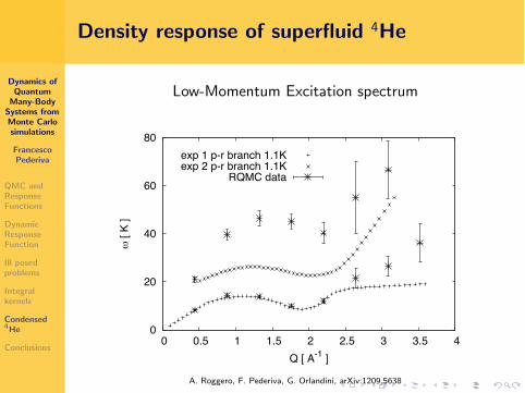
Low-Momentum Excitation spectrum
0
20
40
60
80
0 0.5 1 1.5 2 2.5 3 3.5 4
ω [
K ]
Q [ A-1 ]
exp 1 p-r branch 1.1Kexp 2 p-r branch 1.1K
RQMC data
A. Roggero, F. Pederiva, G. Orlandini, arXiv:1209.5638
Dynamics ofQuantum
Many-BodySystems fromMonte Carlosimulations
FrancescoPederiva
QMC andResponseFunctions
DynamicResponseFunction
Ill posedproblems
Integralkernels
Condensed4He
Conclusions
Density response of superfluid 4He
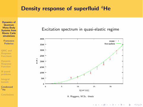
Excitation spectrum in quasi-elastic regime
A. Roggero, M.Sc. thesis

Dynamics ofQuantum
Many-BodySystems fromMonte Carlosimulations
FrancescoPederiva
QMC andResponseFunctions
DynamicResponseFunction
Ill posedproblems
Integralkernels
Condensed4He
Conclusions
Example: density response of superfluid 4He
Excitation spectrum: incoherent (single particle) part
0
10
20
30
40
50
60
0 0.5 1 1.5 2 2.5 3 3.5
ω [
K ]
Q [ A-1 ]
2Δ
Δ
free-particleRQMC data [N=64]
RQMC data [N=125]
A. Roggero, F. Pederiva, G. Orlandini, arXiv:1209.5638

Dynamics ofQuantum
Many-BodySystems fromMonte Carlosimulations
FrancescoPederiva
QMC andResponseFunctions
DynamicResponseFunction
Ill posedproblems
Integralkernels
Condensed4He
Conclusions
Conclusions
Pro
the only input of the calculation is the interaction potential
we only need imaginary-time correlation functions
Con
for high accuracy, extremely long imaginary-time intervalshave to be considered
the inversion procedure still introduces uncontrollableerrors


![Quantum Monte Carlo on geomaterials Dario Alfè [d.alfe@ucl.ac.uk] 2007 Summer School on Computational Materials Science Quantum Monte Carlo: From Minerals](https://img.pdfslide.us/doc/110x75/5697bf951a28abf838c90e05/quantum-monte-carlo-on-geomaterials-dario-alfe-dalfeuclacuk-2007-summer.jpg)