Dynamics of quantum causal structures

Esteban Castro-Ruiz,1, 2 Flaminia Giacomini,1, 2 and Časlav Brukner1, 2

1Vienna Center for Quantum Science and Technology (VCQ), Faculty of Physics,University of Vienna, Boltzmanngasse 5, A-1090 Vienna, Austria

2Institute for Quantum Optics and Quantum Information (IQOQI),Austrian Academy of Sciences, Boltzmanngasse 3, A-1090 Vienna, Austria

It was recently suggested that causal structures are both dynamical, because of general relativity,and indefinite, due to quantum theory. The process matrix formalism furnishes a framework forquantum mechanics on indefinite causal structures, where the order between operations of locallaboratories is not definite (e.g. one cannot say whether operation in laboratory A occurs before orafter operation in laboratory B). Here we develop a framework for “dynamics of causal structures”,i.e. for transformations of process matrices into process matrices. We show that, under continuousand reversible transformations, the causal order between operations is always preserved. However,the causal order between a subset of operations can be changed under continuous yet nonreversibletransformations. An explicit example is that of the quantum switch, where a party in the past affectsthe causal order of operations of future parties, leading to a transition from a channel from A to B, viasuperposition of causal orders, to a channel from B to A. We generalise our framework to constructa hierarchy of quantum maps based on transformations of process matrices and transformationsthereof.

I. INTRODUCTION

We are used to the fact that events occur in a fixed temporal order. Given two events A and B, either A is in thecausal past of B, A is in the causal future of B, or they are causally disconnected (spacelike separated). Althoughthis picture seems natural, the idea that a fixed causal structure is a fundamental ingredient of the physical worldhas been recently challenged. Indeed, the interplay between quantum mechanics and general relativity suggests thatcausality might be indefinite. Because the causal structure in general relativity is determined by a dynamical field –the space-time metric – and dynamical quantities can be indefinite in quantum mechanics (i.e. put in superpositionsof well-defined classical values), one might expect indefiniteness with respect to the question of whether an intervalbetween two events is timelike, null or spacelike, or even whether event A is before or after event B. In order todescribe causal structures that are both dynamical, because of general relativity, and indefinite, due to quantumtheory, several authors have proposed extensions to quantum theory that do not assume a definite causal structure[1–3].

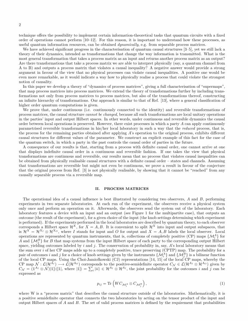
The process matrix formalism [3–6] achieves such a goal. Its central notion is that of a “process” (or a “processmatrix”), which is a generalisation of the notion of a “physical state” (degrees of freedom over a spacelike hypersurface)and of a “channel” (degrees of freedom over a timelike hypersurface). The operational framework in which processmatrices are defined is depicted in Fig. (1). In the framework, observers perform experiments in their local laboratories,where quantum mechanics is assumed to hold. The process matrix is the object that “wires” or “connects” localoperations together, specifying the causal order (definite or indefinite) between such operations. Roughly speaking,it accounts for all the physical processes outside the local laboratories. Process matrices composed with the localoperations form “closed” systems. This means that the probabilities for the events described in the laboratories arecompletely determined by the choice of local operations performed by the parties and the way the process matrixconnects the laboratories. In a closed system, the probabilities do not depend on any “external” operation. Becauseof this independence, this definition of a closed system matches the usual notion of a closed system in physics, in thesense that there is no physical interaction between the system and everything external to it. We say that a compositionof operations has no “open ends” if it is a closed system. A process matrix connected with local operations generalisesthe notion of a quantum circuit [7], and reduces to it in the case where the causal order between the laboratories isfixed.

A process is called causally separable if it can be written as a probabilistic (convex) mixture of states and channels.In the most general scenario, whether a party A can signal to a party B might depend on the choice of operation of yetanother party C, and a general notion of causal nonseparability is required to incorporate these cases [5, 8]. Causallynon-separable processes can give rise to correlations that can violate “causal inequalities”, which are satisfied if theevents are ordered according to a fixed causal order [5, 8]. This is a direct analogy to the violation of Bell’s inequalitiesby quantum correlations, which are satisfied if the correlations fulfil the condition of local causality [9]. While we stilllack an understanding as to whether there are correlations in nature that can violate causal inequalities, we do knowthat physically implementable causally non-separable processes exist. One particular case is the “quantum switch”, anauxiliary quantum system that can coherently control the order in which operations are applied. The quantum-switch

arX

iv:1

710.

0313

9v2

[qu

ant-

ph]

26

Mar

201

8

2

technique offers the possibility to implement certain information-theoretical tasks that quantum circuits with a fixedorder of operations cannot perform [10–12]. For this reason, it is important to understand how these processes, asuseful quantum information resources, can be obtained dynamically, e.g. from separable process matrices.We have achieved significant progress in the characterisation of quantum causal structures [3–5], yet we still lack a

theory of their dynamics, intended as transformations that change the way information is transmitted. What is themost general transformation that takes a process matrix as an input and returns another process matrix as an output?Are there transformations that take a process matrix we are able to interpret physically (say, a quantum channel fromA to B) and outputs a process matrix that violates a causal inequality? A negative answer would provide a strongargument in favour of the view that no physical processes can violate causal inequalities. A positive one would beeven more remarkable, as it would indicate a way how to physically realise a process that could violate the strongestnotion of causality.

In this paper we develop a theory of “dynamics of process matrices”, giving a full characterisation of “supermaps”,that map process matrices into process matrices. We extend the theory of transformations further by including trans-formations not only from process matrices to process matrices, but also of the transformations thereof, constructingan infinite hierarchy of transformations. Our approach is similar to that of Ref. [13], where a general classification ofhigher order quantum computations is given.

We prove that, under continuous (i.e. continuously connected to the identity) and reversible transformations ofprocess matrices, the causal structure cannot be changed, because all such transformations are local unitary operationsin the parties’ input and output Hilbert spaces. In other words, under continuous and reversible dynamics the causalorder between local operations is preserved. However, there exist processes in which a party A can apply continuouslyparametrised reversible transformations in his/her local laboratory in such a way that the reduced process, that is,the process for the remaining parties obtained after applying A’s operation to the original process, exhibits differentcausal structures for different values of the parameter. We construct an explicit example of this fact for the case ofthe quantum switch, in which a party in the past controls the causal order of parties in the future.

A consequence of our results is that, starting from a process with definite causal order, one cannot arrive at onethat displays indefinite causal order in a continuous and reversible fashion. If one takes the view that physicaltransformations are continuous and reversible, our results mean that no process that violates causal inequalities canbe obtained from physically realisable causal structures with a definite causal order – states and channels. Assumingthat transformations are reversible but might not even be continuous, we prove a result in favour of the conjecturethat the original process from Ref. [3] is not physically realisable, by showing that it cannot be “reached” from anycausally separable process via a reversible map.

II. PROCESS MATRICES

The operational idea of a causal influence is best illustrated by considering two observers, A and B, performingexperiments in two separate laboratories. At each run of the experiment, the observers receive a physical systemonly once and perform an operation on it. Afterwards, the observers send the system out of the laboratory. Eachlaboratory features a device with an input and an output (see Figure 1 for the multipartite case), that outputs anoutcome (the result of the experiment), for a given choice of the input (the knob settings determining which experimentis performed). If the experiments performed in the local laboratories are described by quantum theory, to each observercorresponds a Hilbert space HX , for X = A,B. It is convenient to split HX into input and output subspaces, thatis HX = HXI ⊗ HXO , where I stands for input and O for output and X = A,B labels the local observer. Localoperations are represented by quantum instruments, that is, collections of completely positive (CP) maps {MA

i } forA and {MB

j } for B that map systems from the input Hilbert space of each party to the corresponding output Hilbertspace, yielding outcomes labeled by i and j. The conservation of probability in, say, A’s local laboratory means thatthe sum over i of her CP maps adds up to a completely positive, trace preserving (CPTP) map. The probability for apair of outcomes i and j for a choice of knob settings given by the instruments {MA

i } and {MBj } is a bilinear function

of the local CP maps. Using the Choi-Jamiołkowski (CJ) representations [14, 15] of the local CP maps, whereby theCP map N : L(HAI ) −→ L(HAO ) corresponds to the positive-semidefinite operator CN ∈ L(HAI ⊗ HAO ) given byCN = (1AI ⊗ N )|1〉〉〈〈1|, where |1〉〉 =

∑i |ii〉 ∈ HAI ⊗ HAI , the joint probability for the outcomes i and j can be

expressed as

pij = Tr(WCMA

i⊗ CMB

j

), (1)

where W is a “process matrix” that describes the causal structure outside of the laboratories. Mathematically, it isa positive semidefinite operator that connects the two laboratories by acting on the tensor product of the input andoutput Hilbert spaces of A and B. The set of valid process matrices is defined by the requirement that probabilities

3

A

B C

D

a)

A

B C

D

b)

A

B C

D

c)

A

D

B C

d)

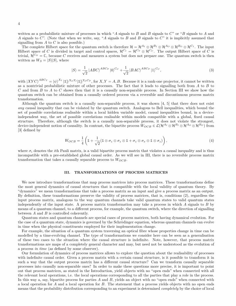
FIG. 1. Composition of local operations. A, B, C and D are local laboratories where the usual quantum formalism holds. Thewires entering and leaving the laboratories represent quantum systems on which operations are applied. a) Local operationsare composed to form a system with definite causal structure and open ends (wires whose ends are not attached to any box).Information flows from bottom to top and the wiring determines the order of operations but is not enough to determine theprobabilities for outcomes of local experiments, because these may change under the influence of external systems through thepast open end. b) A quantum circuit: Local operations are composed with a causally ordered process to yield an object withno open ends. The probabilities for local experiments are determined completely by the choice of local operation and the wiringbetween boxes. c) Composition of local operations with indefinite causal structure. The order of application of operations Band C is not defined a priori. Due to the open end in the past, the causal order and the probabilities depend in general on anexternal system entering through the open end. d) The composition of local operations with a process matrix yields an objectwith indefinite causality and no open ends. The probabilities are determined completely by the choice of local operation andthe process matrix (depicted by the blue E-shaped object) connecting the boxes. The object obtained from the composition isthe generalisation of a quantum circuit for the case where the causal order is indefinite.

are well defined – that is, they must be non negative and add up to 1. These requirements are equivalent to thefollowing constrains:

W ≥ 0 (2a)Tr (W ) = dO (2b)P (W ) = W, (2c)

where dO is the dimension of the output Hilbert space and P is a self-adjoint real projection operator. This operator,first specified in [4], is written explicitly in Appendix A. Physically, conditions (2) exclude Deutsch’s [16] and Lloyd’s[17] closed time-like curves or any causal loops that would allow a party to send a signal into her/his past and hencegive rise to the so-called “grandfather paradox” [5, 18, 19].

Process matrices, i.e. matricesW ∈ L(H) satisfying (2) contain quantum states and quantum channels as particularcases. Concretely, a process matrix of the form W = ρAIBI ⊗ 1AOBO , where ρAIBI is a unit trace, positive matrix,represents the situation in which A and B share a quantum state. A process matrix W = WAIBIAO ⊗ 1BO , whereWAIBIAO is a matrix such that conditions (2) are satisfied, represents a channel (possibly with memory) from A toB. A channel from B to A has an analogous form but with A and B interchanged. A bipartite process matrix Wis called causally ordered if it is either a state shared by A and B, a channel from A to B or a channel from B toA. We can also think of situations in which the process has a definite causal order, but for which only probabilisticpredictions can be made regarding which causal order is realised. To capture this situation, we define a process to becausally separable if it is a probabilistic (convex) mixture of causally ordered processes.

An example of a causally non-separable process is the quantum switch. In the switch, two parties, A and B, act ona target quantum system in an order which is coherently controlled by another quantum system. In order to accountfor the target and control quantum systems as well as for the parties A and B, the quantum switch is formally atripartite process matrix, with the third party, C, being always in the future of A and B. It is reasonable to extendthe definition of causal separability for this case in exactly the same way as for the bipartite case, precisely becauseA and B can always signal to C but C cannot signal to them. We say that a process is causally separable if it can be

4

written as a probabilistic mixture of processes in which “A signals to B and B signals to C” or “B signals to A andA signals to C”. (Note that when we write, say, “A signals to B and B signals to C” it is implicitly assumed thatsignalling from A to C is also possible.)

The complete Hilbert space for the quantum switch is therefore H = HAI ⊗HBI ⊗HAO ⊗HBO ⊗HCI . The inputHilbert space of C is divided in target and control spaces, HCI = HCT ⊗ HCC . The output Hilbert space of C istrivial, HCO = C, because C receives and measures a system but does not prepare one. The quantum switch is thenwritten as WS = |S〉〈S|, where

|S〉 = 1√2|ABC〉ABCT |0〉CC + 1√

2|BAC〉ABCT |1〉CC , (3)

with |XY C〉ABCT = |ψ〉XI |1〉〉XOYI |1〉〉YOCT , for X,Y = A,B. Because it is a rank-one projector, it cannot be writtenas a nontrivial probabilistic mixture of other processes. The fact that it leads to signalling both from A to B toC and from B to A to C shows then that it is a causally non-separable process. In Section III we show how thequantum switch can be obtained from a causally ordered process via a reversible and discontinuous process matrixtransformation.Although the quantum switch is a causally non-separable process, it was shown [4, 5] that there does not exist

any causal inequality that can be violated by the quantum switch. Analogous to Bell inequalities, which bound theset of possible correlations realisable within a local hidden variable model, causal inequalities bound, in a device-independent way, the set of possible correlations realisable within models compatible with a global, fixed causalstructure. Therefore, although the switch is a causally non-separable process, it does not violate the strongest,device-independent notion of causality. In contrast, the bipartite process WOCB ∈ L(HAI ⊗HBI ⊗HAO ⊗HBO ) from[3] defined by

WOCB = 14

(1 + 1√

2(1⊗ σz ⊗ σz ⊗ 1 + σz ⊗ σx ⊗ 1⊗ σz)

), (4)

where σi denotes the ith Pauli matrix, is a valid bipartite process matrix that violates a causal inequality and is thusincompatible with a pre-established global causal order. As we will see in III, there is no reversible process matrixtransformation that takes a causally separable process to WOCB .

III. TRANSFORMATIONS OF PROCESS MATRICES

We now introduce transformations that map process matrices into process matrices. These transformations definethe most general dynamics of causal structures that is compatible with the local validity of quantum theory. By“dynamics” we mean transformations that take a process matrix as an input and give a process matrix as an output.By definition, these transformations preserve the validity of process matrices, that is, conditions (2), regardless theinput process matrix, analogous to the way quantum channels take valid quantum states to valid quantum statesindependently of the input state. A process matrix transformation may take a process in which A signals to B bymeans of a quantum channel, to a different process, for example, the quantum switch, where the direction of signallingbetween A and B is controlled coherently.Quantum states and quantum channels are special cases of process matrices, both having dynamical evolution. For

the case of a quantum state, dynamics is governed by the Schrödinger equation, whereas quantum channels can evolvein time when the physical constituents employed for their implementation change.

For example, the situation of a quantum system traversing an optical fibre whose properties change in time can bemodelled by a time-evolving channel. The type of transformations we consider here can be seen as a generalisationof these two cases to the situation where the causal structure is indefinite. Note, however, that process matrixtransformations are maps of a completely general character and may, but need not be understood as the evolution ofa process in time (as defined by some observer).Our formulation of dynamics of process matrices allows to explore the question about the realisability of processes

with indefinite causal order. Given a process matrix with a certain causal structure, is it possible to transform it insuch a way that the output process matrix has a different causal structure? Can we transform causally separableprocesses into causally non-separable ones? In order to make these questions more precise, it is important to pointout that process matrices, as stated in the Introduction, yield objects with no “open ends” when connected with allthe relevant local operations, i.e. the local operations corresponding to all the parties that play a role in the process.In this way a, say, bipartite process for parties A and B, yields an object with no “open ends” when connected witha local operation for A and a local operation for B. The statement that a process yields objects with no open endsmeans that the probability distribution corresponding to an experiment is determined completely by the choice of local

5

operations made by the parties and the way these local operations are “wired” together. Just to be clear: The waywe have defined objects, it is not the process matrix that has no open ends but rather the composition of the processmatrix with the relevant local operations. For the case of quantum circuits [7], the wiring of the boxes, togetherwith the convention that information flows from bottom to top, determines the order in which the operations areapplied, see Fig. (1a) and (1b). For the more general case of an indefinite causal structure, in which the order of localoperations is not fixed in principle, the wiring of the boxes is replaced by “E-shaped” objects (see Fig. (1c) and (1d)),that specify the causal structure (definite or indefinite) outside the local laboratories. For an object with indefinitecausality and open ends, (Fig. (1)c), the notion of causal non separability is in general not well defined, because thesignalling between the parties is, in the general case, determined not only by their choice of local operations and the“E-shaped” object outside the laboratories, but also by the external systems influencing the experiment via the openends. In some cases, the natural way to proceed in this case is to “close” the wires by inserting local laboratories ateach open end, and study the causal (non)separability of the process matrix thus obtained. Note that this processmatrix will have more parties than the original “E-shaped” object, and the question whether it is causally separableor not has to be analysed considering the newly added parties.

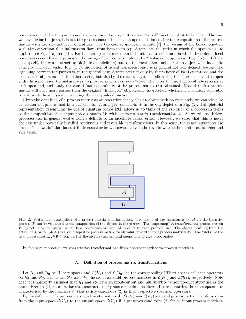
Given the definition of a process matrix as an operation that yields an object with no open ends, we can visualisethe action of a process matrix transformation A on a process matrix W in the way depicted in Fig. (2). This pictorialrepresentation, resembling the one of quantum combs [20], allows us to think of the evolution of a process in termsof the composition of an input process matrix W with a process matrix transformation A. As we will see below,processes can in general evolve from a definite to an indefinite causal order. However, we show that this is neverthe case under physically justified continuous and reversible transformations. In this sense, the causal structures are“robust”: a “world” that has a definite causal order will never evolve in in a world with an indefinite causal order andvice versa.

W

A

FIG. 2. Pictorial representation of a process matrix transformation. The action of the transformation A on the bipartiteprocess W can be visualised as the composition of the objects in the picture. The “supermap” A transforms the process matrixW by acting on its “slots”, where local operations are applied in order to yield probabilities. The object resulting from theaction of A on W , A(W ) is a valid bipartite process matrix for all valid bipartite input process matrices W . The “slots” of thenew process matrix A(W ) (top part of the picture) act on local operations to give probabilities.

In the next subsection we characterise transformations from process matrices to process matrices.

A. Definition of process matrix transformations

Let H1 and H2 be Hilbert spaces and L(H1) and L(H2) be the corresponding Hilbert spaces of linear operatorson H1 and H2. Let us call W1 and W2 the set of all valid process matrices in L(H1) and L(H2), respectively. Notethat it is implicitly assumed that H1 and H2 have an input-output and multipartite tensor product structure as theone in Section (II) to allow for the construction of process matrices on them. Process matrices in these spaces arecharacterised by the matrices W that satisfy conditions (2) in their respective spaces of operators.By the definition of a process matrix, a transformationA : L(H1) −→ L(H2) is a valid process matrix transformation

from the input space L(H1) to the output space L(H2) if it preserves conditions (2) for all input process matrices.

6

Let us analyse what each of these conditions imply for A. Condition (2a) implies that A is a positive map. As for thecase of quantum states, it is physically meaningful to consider process matrix transformations that act on a propersubset of the parties of a multipartite process. Moreover, it is also physically sound that the complete set of partiesof the transformed process can share entangled quantum systems. As we show in Appendix B, these requirementsimply that the map A is completely positive. An alternative proof of complete positivity can be found in Ref. [13].Condition (2b) implies that A must be trace rescaling, that is, it must rescale the trace of the input process matrixdO1 to the dimension of the space HO2 , dO2 . Because this condition has to be satisfied for all process matrices, A mustbe of the form A = dO

2dO

1A, where A is a trace preserving map. In particular, if the input space is isomorphic to the

output space, then A is a completely positive trace preserving map. Requiring that A preserves (2c) is equivalent torequiring

P2 ◦ A ◦ P1 = A ◦ P1, (5)

where the subindices in the projector P of (2c) indicate that the input and output space may be different. This generalrequirement captures not only the case where the dimension of the Hilbert spaces in which the parties act changesafter the transformation, but also the case where the number of parties is different before and after the transformation.

In order to relate the conditions implied for A and conditions (2), it is convenient to rewrite the conditions for Ain terms of its CJ operator, CA. The first two conditions for A can be rewritten in a straightforward way using thewell-known properties of the CJ operator (see, for example, [21]):

• A is completely positive if and only if CA ≥ 0

• A is trace-rescaling if and only if Tr2 (CA) = dO2dO

111,

where the subindices 1 and 2 refer, respectively, to the Hilbert spaces H1 and H2.In order to write the third condition in terms of CA, we take the CJ operator of the right hand side of (5). Using

the fact that 1⊗N (|1〉〉〈〈1|) = N T ⊗1(|1〉〉〈〈1|) (the superscript T denotes transpose with respect to the basis in which|1〉〉 ∈ H1 ⊗H1 is defined), we find

1⊗A ◦ P1(|1〉〉〈〈1|) =PT1 ⊗ 1(CA). (6)

On the other hand, taking the CJ of the left hand side of (5) gives

1⊗ P2 ◦ A ◦ P1(|1〉〉〈〈1|) = PT1 ⊗ P2(CA).

As noted in Section II, and as can be explicitly seen in Appendix A, P1 is a real projector. Being hermitian, it equalsits transpose, P1 = PT1 . Therefore we can rewrite condition (5) as

P1 ⊗ 1(CA) = P1 ⊗ P2(CA) (7)

We have then written all conditions for A in terms of its CJ, CA. In summary, we have characterised all the possibletransformations that take any valid process matrix to another valid process matrix in terms of their CJ representation.Process matrix transformations A have CJ representations that satisfy the following:

CA ≥0 (8a)

Tr2 (CA) =dO2dO1

11 (8b)

P1 ⊗ 1(CA) =P1 ⊗ P2(CA). (8c)

B. Higher order maps

In this section we show how the idea of process matrix transformations can be generalised to the case of higherorder transformations, thereby extending the framework of process matrices, which, as we show in this Section, canbe seen as transformations of order 1. First, we note that condition (7) can be written as

(1⊗ 1− P1 ⊗ 1 + P1 ⊗ P2)(CA) = CA. (9)

This is convenient because condition (7) is rephrased in terms of a projection operator that leaves CA invariant. Moreprecisely, the supermap A has an input space H1 and an output space H2. Its CJ operator CA ∈ L(H1 ⊗ H2) is

7

invariant under the projector P (2)12 := 1⊗ 1−P1 ⊗ 1 +P1 ⊗P2. Condition (9) is a generalisation of condition (2c) for

process matrices. More concretely, we note that any process matrix W can be considered to be the CJ of a supermapwith a trivial input space H1 = C. To see that this is the case we rewrite the condition (7) for W . We get

(1⊗ 1− 1⊗ 1 + 1⊗ P )(W ) = P (W ) = W, (10)

which is just the original condition (2c) we know for W . In this sense, W is a particular type of supermap, withtrivial input space.

We can now generalise the projector (9) to build a hierarchy of higher-order transformations, in the spirit of Ref.[13]. We define P (1)

1 = P1, P (1)2 = P2 and

P(n)12 = 1⊗ 1− P (n−1)

1 ⊗ 1 + P(n−1)1 ⊗ P (n−1)

2 . (11)

From this point of view a process matrix W =: W1 is a supermap of order 1 in the sense that it satisfies P1(W1) = W1(together with the positivity and trace-preserving condition). A map A that takes a process matrix to a processmatrix is a supermap of order 2 in the sense that its CJ, CA satisfies P2(CA) = CA (together with the positivityand trace-rescaling condition). In this way we can define these type of maps for arbitrary order, that is, a supermapof order n, Wn ∈ Wn is an operator that satisfies P (n)

12 (Wn) = Wn (together with the positivity and trace-rescalingcondition). It takes a valid supermap of order n − 1, with corresponding Hilbert space H1, to a valid supermap oforder n− 1 with corresponding Hilbert space H2.

IV. CONTINUOUS AND REVERSIBLE TRANSFORMATIONS PRESERVE THE CAUSAL ORDER OFA PROCESS

In this Section we formulate and state the main result of our paper, namely, that the causal structure of a processremains invariant under continuous and reversible dynamics. Consider a bipartite process matrix with a correspondingHilbert space H = HAI ⊗HAO ⊗HBI ⊗HBO . Let U : L(H) −→ L(H) be a continuous, i.e. continuously connectedto the identity, and reversible transformation from process matrices to process matrices. Concretely, the continuityand reversibility requirements for U mean that there exists a one-parameter family of valid, reversible process matrixtransformations Uλ, such that Uλ=0 is the identity transformation and Uλ=1 = U . Since, by assumption, Uλ is a validprocess matrix transformation for all λ, it is a CPTP map for all λ. Moreover, since Uλ has an inverse for all λ andthe inverse is also a valid process matrix transformation, there exists a family of unitary matrices Uλ = e−iλH , forsome traceless, hermitian operator H, such that Uλ(X) = UλXU†λ for all X ∈ L(H). As a consequence, the conditionfor U(λ) to be a valid process matrix transformation is P (e−iλHW eiλH) = e−iλHW eiλH for all W ∈ W, where wehave omitted the subindices in the operator P because the input and output Hilbert spaces are isomorphic. If we takeλ to be infinitesimal, the condition above reads P (W − iλ [H,W ]) = P (W ) − iλP ([H,W ]) = W − iλP ([H,W ]) =W − iλ [H,W ], where we have used the fact that W is a valid process matrix. From this we conclude that

P ([H,W ]) = [H,W ] . (12)

In Appendix C, we show that condition (12) can only be satisfied by local unitaries, that is, unitaries of the form

U = U IA ⊗ U IB ⊗ UOA ⊗ UOB , (13)

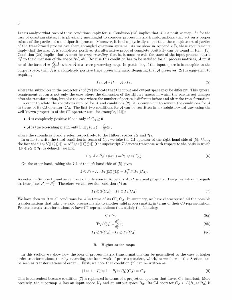
and we generalise the proof for an arbitrary number of parties and dimensions of the local laboratories’ systems.In conclusion, ifW is any process matrix and U is a continuous and reversible process matrix transformation, in the

sense specified above, then U is merely a product of local unitaries, of the form of Eq. (13), see Fig. (3). Importantly,this fact implies that the causal structure of W remains unchanged under the action of U . This result points to theidea that causality is a robust feature of physical processes: any transformation that changes the causal order of aprocess must be either discontinuous or irreversible.

V. EXAMPLES

Let us now consider some interesting examples of process matrix transformations.

8

W

A B

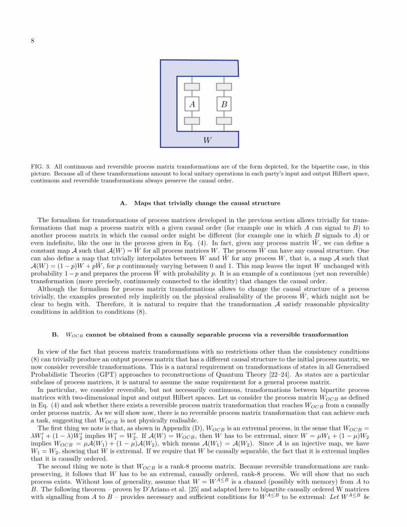
FIG. 3. All continuous and reversible process matrix transformations are of the form depicted, for the bipartite case, in thispicture. Because all of these transformations amount to local unitary operations in each party’s input and output Hilbert space,continuous and reversible transformations always preserve the causal order.

A. Maps that trivially change the causal structure

The formalism for transformations of process matrices developed in the previous section allows trivially for trans-formations that map a process matrix with a given causal order (for example one in which A can signal to B) toanother process matrix in which the causal order might be different (for example one in which B signals to A) oreven indefinite, like the one in the process given in Eq. (4). In fact, given any process matrix W , we can define aconstant map A such that A(W ) = W for all process matricesW . The process W can have any causal structure. Onecan also define a map that trivially interpolates between W and W for any process W , that is, a map A such thatA(W ) = (1− p)W + pW , for p continuously varying between 0 and 1. This map leaves the input W unchanged withprobability 1− p and prepares the process W with probability p. It is an example of a continuous (yet non reversible)transformation (more precisely, continuously connected to the identity) that changes the causal order.

Although the formalism for process matrix transformations allows to change the causal structure of a processtrivially, the examples presented rely implicitly on the physical realisability of the process W , which might not beclear to begin with. Therefore, it is natural to require that the transformation A satisfy reasonable physicalityconditions in addition to conditions (8).

B. WOCB cannot be obtained from a causally separable process via a reversible transformation

In view of the fact that process matrix transformations with no restrictions other than the consistency conditions(8) can trivially produce an output process matrix that has a different causal structure to the initial process matrix, wenow consider reversible transformations. This is a natural requirement on transformations of states in all GeneralisedProbabilistic Theories (GPT) approaches to reconstructions of Quantum Theory [22–24]. As states are a particularsubclass of process matrices, it is natural to assume the same requirement for a general process matrix.

In particular, we consider reversible, but not necessarily continuous, transformations between bipartite processmatrices with two-dimensional input and output Hilbert spaces. Let us consider the process matrix WOCB as definedin Eq. (4) and ask whether there exists a reversible process matrix transformation that reachesWOCB from a causallyorder process matrix. As we will show now, there is no reversible process matrix transformation that can achieve sucha task, suggesting that WOCB is not physically realisable.The first thing we note is that, as shown in Appendix (D),WOCB is an extremal process, in the sense thatWOCB =

λW ′1 + (1 − λ)W ′2 implies W ′1 = W ′2. If A(W ) = WOCB , then W has to be extremal, since W = µW1 + (1 − µ)W2implies WOCB = µA(W1) + (1 − µ)A(W2), which means A(W1) = A(W2). Since A is an injective map, we haveW1 = W2, showing thatW is extremal. If we require thatW be causally separable, the fact that it is extremal impliesthat it is causally ordered.

The second thing we note is that WOCB is a rank-8 process matrix. Because reversible transformations are rank-preserving, it follows that W has to be an extremal, causally ordered, rank-8 process. We will show that no suchprocess exists. Without loss of generality, assume that W = WA≤B is a channel (possibly with memory) from A toB. The following theorem – proven by D’Ariano et al. [25] and adapted here to bipartite causally ordered W matriceswith signalling from A to B – provides necessary and sufficient conditions for WA≤B to be extremal: Let WA≤B be

9

a causally ordered process matrix and let supp(WA≤B) be its support. Let C be a basis of hermitian operators in thespace L(supp(WA≤B)). Define D = {σBI

i σBOµ σAI

ν σAOρ ,1BI 1BOσAI

i σAOµ }, for greek indices running from 0 to 3 and

latin indices from 1 to 3. The process WA≤B is extremal iff the disjoint union C tD is linearly independent.From this theorem it is straightforward to see that there is no extremal, rank-8, causally ordered bipartite process.

The process being rank 8 implies that C has 82 = 64 elements. The set D has 204 elements, which means their disjointunion C tD has 268 elements. The dimension of L(H) is 256, implying that C tD is not linearly independent. Thisshows that WA≤B is not extremal. We conclude that WOCB cannot be obtained reversibly from a causally orderedprocess. Note that the restrictions we impose on the transformations in this example are weaker than those leading toour result in IV, that is, we ask for the transformations to be reversible but not necessarily continuous. Nevertheless,as we have shown, the process (4) cannot be obtained by transforming a causally ordered one, even without thecontinuity restriction.

C. C-SWAP transformation: obtaining the quantum switch from a channel

We have shown that the process matrix (4) cannot be obtained from a causally ordered process via a reversibletransformation. We will now show that this is not the case for the quantum switch: There exists a reversible processmatrix transformation that takes a causally ordered process (a channel in one direction) to the quantum switch.

Consider the Hilbert space corresponding to the quantum switch H = HAI ⊗ HBI ⊗ HAO ⊗ HBO ⊗ HCT ⊗ HCC

and the transformation

V = 1ABCT ⊗ |0〉〈0|CC + SWAPAB ⊗ 1CT ⊗ |1〉〈1|CC , (14)

where for simplicity of notation we have written A to denote the Hilbert space HA = HAI ⊗HAO and similarly for B.We define SWAPAB = SWAPAI BI⊗SWAPAO BO where the well-known SWAP operator acts as SWAP |ψ〉⊗ |φ〉 =|φ〉⊗ |ψ〉. The transformation V is a proper process matrix transformation in the sense that it obeys the conditions(8), and yields the quantum switch when acting on the channel |ABC〉ABCT |+〉CC , with the notation used in (3) and|+〉 = (|0〉+ |1〉)

√2:

V |ABC〉ABCT |+〉CC = 1√2|ABC〉ABCT |0〉CC + 1√

2|BAC〉ABCT |1〉CC = |S〉 . (15)

The transformation V is a reversible supermap that takes a causally separable process as an input (a quantumchannel) to a causally non-separable process (the quantum switch). One could ask if this transformation can be castin such a way that it is also continuous, i.e. if there exists a continuously parametrised set of supermaps that reducesto V for some value of the parameter and to the identity for some other value. A seemingly good candidate is thetransformation Vλ = exp(−iλH), for H = (SWAPAI BI ⊗ SWAPAO BO − 1AI BI ⊗ 1AO BO ) ⊗ 1CT ⊗ |1〉〈1|CC . Thistransformation reduces to the identity for λ = 0 and to V for λ = π/2. However, applying Vλ to the process vector|ABC〉ABCT |1〉CC yields Vλ |ABC〉ABCT |1〉CC = exp(iλ)(cosλ |ABC〉ABCT −i sinλ |BAC〉ABCT ) |1〉CC , which is nota valid process matrix since, as a straightforward calculation shows, it contains, for instance, “forbidden” terms ofthe form σi ⊗ σi ⊗ σi ⊗ σi ⊗ 1 ∈ L(HAI ⊗HBI ⊗HAO ⊗HBO ⊗HCI ). The failure to find a continuous and reversibleprocess matrix transformation that changes the causal structure is a particular instance of the more general resultof Section (IV), namely, that all continuous and reversible transformations of process matrices reduce only to localunitaries in the parties’ input and output Hilbert spaces, showing that no continuous and reversible process matrixtransformation can change the causal structure.

D. Local operations of one party that influence the causal structure of the remaining parties

It is known [5, 8] that, in a general multipartite process matrix, local operations performed by one of the partiescan influence the causal structure of the remaining parties. We will show now that this feature can be expressednaturally in terms of process matrix transformations. Consider an N partite process WN over a Hilbert space HNfor N > 2 and let the X-th party perform a local CPTP map M in his/her laboratory. This will induce an N − 1reduced process matrix WN−1 over the Hilbert space HN−1. The causal order of the reduced process can in generaldepend onM. Define the process matrix transformation AM : L(HN ) −→ L(HN−1) as

AM(W ) = TrX (CMW ) , (16)

where CM denotes the CJ representation of the map M. The supermap AM is a well-defined process matrixtransformation that can in principle yield processes with indefinite causal structure. Note, however, that the process

10

A B

C

D

a)

A B

C

D

b)

A B

C

D

c)

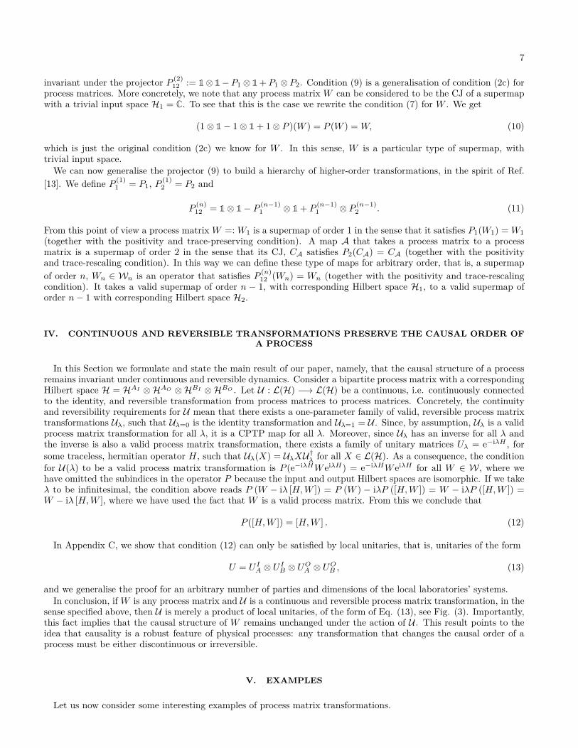
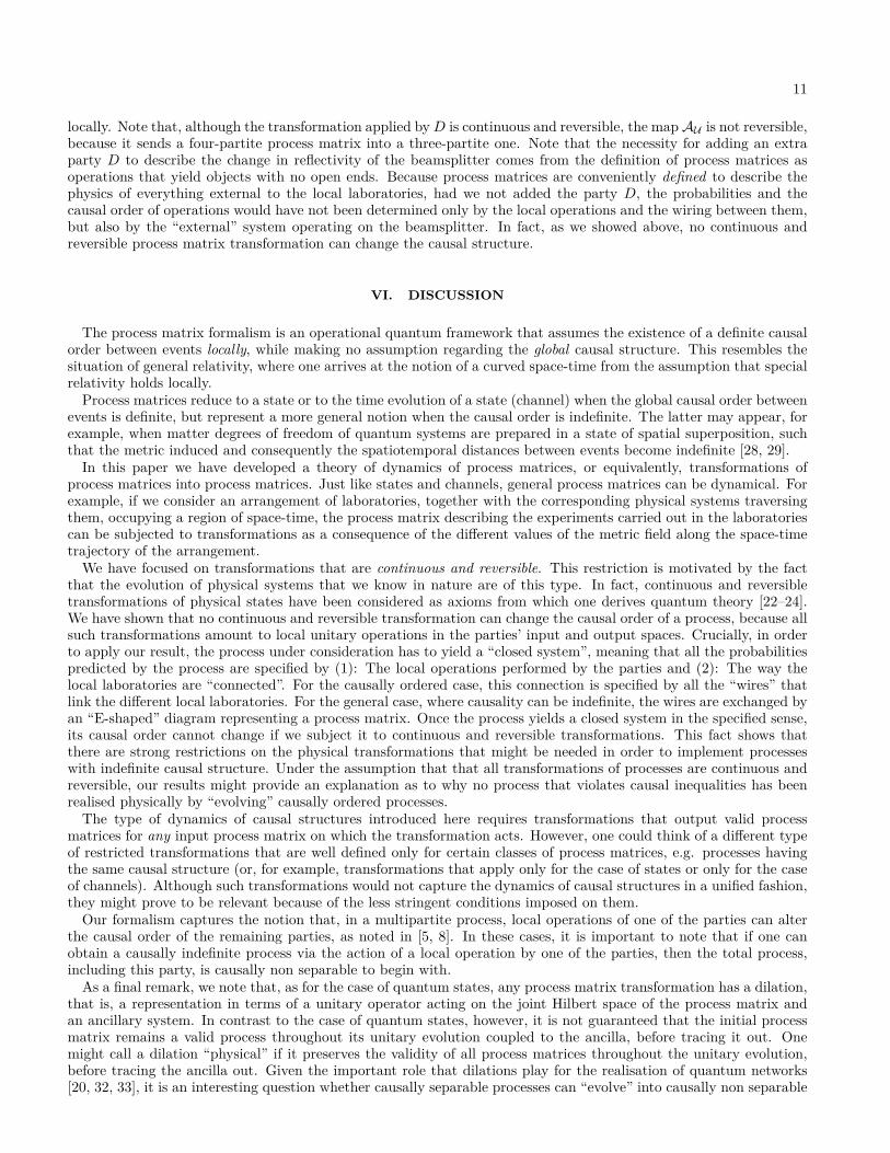
FIG. 4. A four partite process matrix for parties A, B, C and D can be mapped to a continuous family of three partite processesfor parties A, B and C. By choosing different local operations for D, one can map the four partite input process matrix toprocesses that exhibit different causal order. In a concrete quantum optical realisation of this transformation, D controls thereflectivity of a beam splitter (see main text). The transformation can go continuously from a) a channel from A to B to C toc) a channel from B to A to C, passing through c) the quantum switch (see Eq. (3)).

WN−1 being causally non separable implies that the process WN itself is also causally non separable. To see this,suppose that WN is causally separable. This means that for any choice of local operations, the resulting multipartiteexperiment can always be explained in terms of a convex combination of states and channels. This fact holds for theparticular case in which the X-th party chooses to apply the mapM. But this choice would imply that the processWN−1 is causally separable, contradicting our initial assumption.Let us now analyse a concrete example of a process matrix transformation where the action of a party in the past

decides the direction of the signalling of parties in the future. This party can even decide whether the remaining processis causally separable or not. Our example, depicted in Fig. (4) is motivated by the experimental implementation ofthe quantum switch in an optical setup [26, 27]. In this experiment, a photon traverses a beam splitter that dividesits trajectory into two paths. In one path the local operation MA is applied to the polarisation degree of freedomof the photon before local operation MB , while the other path corresponds to exactly the opposite: The operationMB is followed byMA. By continuously changing the reflectivity of the beamsplitter, we can go continuously from asituation in which A signals to B to the situation in which B signals to A, passing through an intermediate situationthe corresponds to the quantum switch.Formally, the action of changing the reflectivity of the beamsplitter corresponds to adding an extra party D to the

quantum switch (3). The initial process W that we consider has therefore a Hilbert space H = HAI ⊗HBI ⊗HDI ⊗HAO ⊗HBO ⊗HDO ⊗HCT ⊗HCC . W is given by W = |W 〉〈W |, where

|W 〉 = |ABC〉ABCT |0〉DI |0〉DO |0〉CC + |BAC〉ABCT |0〉DI |1〉DO |1〉CC , (17)

using the same notation as in Eq. (3). We consider the case in which D performs a unitary map U : HDI −→ HDO

defined as U(ρ) = UρU†, specified by the matrix

U =(

cosλ − sinλsinλ cosλ

). (18)

The output process is obtained when D acts locally with U . This defines a supermap AU in the sense described above.Its action on W yields AU (W ) = TrD (CUW ) = |Wλ〉〈Wλ|, where

|Wλ〉 = cosλ |ABC〉ABCT |0〉CC + sinλ |BAC〉ABCT |1〉CC . (19)

|Wλ〉 is a channel from A to B for λ = 0, reduces to the quantum switch for λ = π/2, and to a channel from B to Afor λ = π. The party D can change the causal structure of the remaining three parties by applying a transformation

11

locally. Note that, although the transformation applied byD is continuous and reversible, the mapAU is not reversible,because it sends a four-partite process matrix into a three-partite one. Note that the necessity for adding an extraparty D to describe the change in reflectivity of the beamsplitter comes from the definition of process matrices asoperations that yield objects with no open ends. Because process matrices are conveniently defined to describe thephysics of everything external to the local laboratories, had we not added the party D, the probabilities and thecausal order of operations would have not been determined only by the local operations and the wiring between them,but also by the “external” system operating on the beamsplitter. In fact, as we showed above, no continuous andreversible process matrix transformation can change the causal structure.

VI. DISCUSSION

The process matrix formalism is an operational quantum framework that assumes the existence of a definite causalorder between events locally, while making no assumption regarding the global causal structure. This resembles thesituation of general relativity, where one arrives at the notion of a curved space-time from the assumption that specialrelativity holds locally.

Process matrices reduce to a state or to the time evolution of a state (channel) when the global causal order betweenevents is definite, but represent a more general notion when the causal order is indefinite. The latter may appear, forexample, when matter degrees of freedom of quantum systems are prepared in a state of spatial superposition, suchthat the metric induced and consequently the spatiotemporal distances between events become indefinite [28, 29].

In this paper we have developed a theory of dynamics of process matrices, or equivalently, transformations ofprocess matrices into process matrices. Just like states and channels, general process matrices can be dynamical. Forexample, if we consider an arrangement of laboratories, together with the corresponding physical systems traversingthem, occupying a region of space-time, the process matrix describing the experiments carried out in the laboratoriescan be subjected to transformations as a consequence of the different values of the metric field along the space-timetrajectory of the arrangement.

We have focused on transformations that are continuous and reversible. This restriction is motivated by the factthat the evolution of physical systems that we know in nature are of this type. In fact, continuous and reversibletransformations of physical states have been considered as axioms from which one derives quantum theory [22–24].We have shown that no continuous and reversible transformation can change the causal order of a process, because allsuch transformations amount to local unitary operations in the parties’ input and output spaces. Crucially, in orderto apply our result, the process under consideration has to yield a “closed system”, meaning that all the probabilitiespredicted by the process are specified by (1): The local operations performed by the parties and (2): The way thelocal laboratories are “connected”. For the causally ordered case, this connection is specified by all the “wires” thatlink the different local laboratories. For the general case, where causality can be indefinite, the wires are exchanged byan “E-shaped” diagram representing a process matrix. Once the process yields a closed system in the specified sense,its causal order cannot change if we subject it to continuous and reversible transformations. This fact shows thatthere are strong restrictions on the physical transformations that might be needed in order to implement processeswith indefinite causal structure. Under the assumption that that all transformations of processes are continuous andreversible, our results might provide an explanation as to why no process that violates causal inequalities has beenrealised physically by “evolving” causally ordered processes.

The type of dynamics of causal structures introduced here requires transformations that output valid processmatrices for any input process matrix on which the transformation acts. However, one could think of a different typeof restricted transformations that are well defined only for certain classes of process matrices, e.g. processes havingthe same causal structure (or, for example, transformations that apply only for the case of states or only for the caseof channels). Although such transformations would not capture the dynamics of causal structures in a unified fashion,they might prove to be relevant because of the less stringent conditions imposed on them.

Our formalism captures the notion that, in a multipartite process, local operations of one of the parties can alterthe causal order of the remaining parties, as noted in [5, 8]. In these cases, it is important to note that if one canobtain a causally indefinite process via the action of a local operation by one of the parties, then the total process,including this party, is causally non separable to begin with.

As a final remark, we note that, as for the case of quantum states, any process matrix transformation has a dilation,that is, a representation in terms of a unitary operator acting on the joint Hilbert space of the process matrix andan ancillary system. In contrast to the case of quantum states, however, it is not guaranteed that the initial processmatrix remains a valid process throughout its unitary evolution coupled to the ancilla, before tracing it out. Onemight call a dilation “physical” if it preserves the validity of all process matrices throughout the unitary evolution,before tracing the ancilla out. Given the important role that dilations play for the realisation of quantum networks[20, 32, 33], it is an interesting question whether causally separable processes can “evolve” into causally non separable

12

ones via transformations that have only continuous, physical dilations. In view of the strong restrictions on continuousunitary transformations found in this work, it seems reasonable to conjecture a negative answer to this question. Arigorous proof of this fact is left for future work.

VII. ACKNOWLEDGEMENTS

We thank P. Allard-Guérin, M. Araújo, C. Budroni, F. Costa, P. Perinotti and M. Sedlák for interesting discussions.We acknowledge the support from the Austrian Science Fund (FWF) through the Special Research Programme FoQuS,the Doctoral Programme CoQuS and the project I-2526 and the research platform TURIS. This publication wasmade possible through the support of a grant from the John Templeton Foundation. The opinions expressed in thispublication are those of the authors and do not necessarily reflect the views of the John Templeton Foundation.

[1] Hardy L. Probability theories with dynamic causal structure: a new framework for quantum gravity. Preprint athttps://arxiv.org/abs/gr-qc/0509120 (2005).

[2] Oeckl R. A local and operational framework for the foundations of physics. Preprint at https://arxiv.org/abs/1610.09052(2016).

[3] Oreshkov O, Costa F, Brukner, Č. Quantum correlations with no causal order. Nature Commun. 3 1092 (2012).[4] Araújo M, Branciard C, Costa F, Feix A, Giarmatzi C, Brukner Č. Witnessing causal nonseparability. New J. Phys. 17

102001 (2015).[5] Oreshkov O, Giarmazi C. Causal and causally separable processes. New. J. Phys 18 093020 (2016).[6] Giacomini F, Castro-Ruiz E, Brukner Č. Indefinite causal structures for continuous-variable systems. New J. Phys. 18

113026 (2016).[7] Hardy L. The operator tensor formulation of quantum theory. Phil. Trans. R. Soc. A 370 3385 (2012).[8] Abbott AA, Giarmatzi C, Costa F, Branciard C. Multipartite causal correlations: Polytopes and inequalities. Phys. Rev.

A 94 032131 (2016).[9] Bell JS. On the Einstein Podolsky Rosen Paradox. Physics 1,3 195–200 (1964).

[10] Chiribella G, D’Ariano GM, Perinotti P, Valiron B. Quantum computations without definite causal structure. Phys. Rev.A 88 022318 (2013).

[11] Araújo M, Costa F, Brukner Č. Computational advantage from quantum-controlled ordering of gates. Phys. Rev. Lett.113 250402 (2014).

[12] Guérin PA, Feix A, Araújo M, Brukner Č. Exponential communication complexity advantage from quantum superpositionof the direction of communication. Phys. Rev. Lett. 117 100502 (2016).

[13] Perinotti P. Causal structures and the classification of higher order quantum computations. Preprint athttps://arxiv.org/abs/1612.05099 (2016).

[14] Jamiołkowski A. Linear transformations which preserve trace and positive semidefiniteness of operators. Rep. Math. Phys.3,4, 275–278 (1972).

[15] Choi MD. Completely positive linear maps on complex matrices. Lin. Alg. Appl. 10 285–290 (1975).[16] Deutsch D. Quantum mechanics near closed timelike lines. Phys. Rev. D 44 3197–3217 (1991).[17] Lloyd S. et al. Closed timelike curves via post-selection: theory and experimental demonstration. Phys. Rev. Lett. 106

040403 (2011).[18] Allen JM. Treating time travel quantum mechanically. Phys. Rev. A 90 042107 (2014).[19] Baumeler Ä, Wolf S. Non-Causal Computation. Entropy 19(7) 326 (2017).[20] Chiribella G, D’Ariano GM, Perinotti P. Theoretical framework for quantum networks. Phys. Rev. A 80 022339 (2009).[21] Heinosaari T, Ziman M. The Mathematical Language Quantum Theory: From Uncertainty to Entanglement. Cambridge

University Press (2012).[22] Hardy L. Quantum theory from five reasonable axioms. Preprint at: https://arxiv.org/abs/quant-ph/0101012 (2001).[23] Dakic B, Brukner Č. Quantum Theory and Beyond: Is entanglement special? Deep Beauty - Understanding the Quantum

World through Mathematical Innovation ED. Halvorson, H. (2011).[24] Masanes L, Müller MP. A derivation of quantum theory from physical requirements. New J. Phys. 13 063001 (2011).[25] D’Ariano GM, Perinotti P, and Sedlák M. Extremal Quantum Protocols Jour. Math. Phys 52 082202 (2011).[26] Procopio LM, Moqanaki A, Araújo M, Costa F, Calafell IA, Dowd GE, Hamel DR, Rozema LA, Brukner Č, Walther P.

Experimental superposition of orders of quantum gates. Nat. Commun. 6 7913 (2015).[27] Rubino G, Rozema LA, Feix A, Araújo M, Zeuner JM, Procopio LM, Brukner Č, Walther P. Experimental verification of

an indefinite causal order. Science Advances 3 1602589 (2017).[28] Zych M, Costa F, Pikovski I, Brukner Č. Bell’s Theorem for Temporal Order. Preprint at: https://arxiv.org/abs/1708.00248

(2017).[29] Feix A, Brukner Č. Quantum superpositions of “common-cause” and “direct-cause” causal structures. Preprint at:

https://arxiv.org/abs/1606.09241 (2016).

13

[30] Bengtsson I, Życzowski K. Geometry of Quantum States. Cambridge University Press. (2006).[31] Georgi H. Lie Algebras in Particle Physics: From Isospin to Unified Theories. Westview Press. (1999).[32] Bisio A, D’Ariano GM, Perinotti P and Chiribella G. Minimal computational-space implementation of multiround quantum

protocols Phys. Rev. A 83 022325 (2011).[33] Bisio A, Chiribella G, D’Ariano GM, and Perinotti P. Quantum Networks: General Theory and Applications Acta Physica

Slovaca 61-3 273-390 (2011).

14

Appendix A: Further details on the characterisation of process matrices

In this section we give, for the sake of completeness, a description of the projector P introduced on Section IIin the main text. For our purposes, it suffices to focus on the bipartite case, corresponding to the Hilbert spaceH = HAI ⊗ HBI ⊗ HAO ⊗ HBO . Let the two parties, A and B, perform local operations described by completelypositive (CP) maps MX

i , X = A,B. The label i denotes a possible measurement outcome of the correspondinglocal operation. The CP maps act from the input Hilbert space HXI to the output Hilbert space HXO of eachparty X = A,B. The set of local operations {MX

i }, where i takes values on the set of possible outcomes, form aquantum instrument, that is, they add up to a completely positive, trace preserving (CPTP) map MX =

∑iMX

i .The joint probability for A to obtain outcome i, corresponding to the operationMA

i , and for B to obtain outcome j,corresponding to the operationMB

j , is given by the “generalised Born rule” (Eq. (1)): pij = Tr(WCMA

i⊗ CMB

j

),

where W ∈ L(H) is the process matrix describing the physics outside the local laboratories, and CMXi

denotes theChoi-Jamiołkowski (CJ) representation of the mapMX

k , for X = A,B and k = i, j. The conservation of probabilitymeans that the sum of all probabilities equals unity:

∑ij pij = Tr (WCMA ⊗ CMB ) = 1. It is known that the CJ

representation of a map satisfies TrXOCMX = 1XI if and only if the map MX , X = A,B, is trace preserving.

Therefore, the conservation of probability for process matrices can be stated as

Tr (WCMA ⊗ CMB ) = 1, (A1)

for all CMX , X = A,B, satisfying TrXOCMX = 1XI . It was shown in Refs. [3, 4], that this condition implies, apart

from the normalisation of the trace of W given in Eq. (2b), Tr (W ) = dO, that the process matrix W belongs toa proper subspace of the total Hilbert space of operators L(H). Explicitly, W is invariant under the projector Pintroduced in Ref. [4], given by

P (W ) =AOW +B0W −AIAO

W −BIBOW −AOBO

W +AOBIBOW +BOAIAO

W, (A2)

where XW := d−1X 1X ⊗ TrX(W ) for any subspace X of L(H).

In order to acquire some physical intuition regarding the structure of P , it is useful to write down the elements ofL(H) in terms of the Hilbert-Schmidt basis B = {σα⊗σβ⊗σγ⊗σδ}, where all greek indices run from 0 to d2−1, withd equal to the dimension of a single tensor factor of the total space, for example HAI . For simplicity of notation, weassume that each tensor factor of H is equal to the space Cd. Note that this assumption can be made without losinggenerality, because we can always add dimensions to laboratories with trivial operations. By definition, σ0 =

√2/d1,

and σi is a hermitian, traceless operator for all values of the latin index i, running from 1 to d2− 1. In this basis, theprojector defined in Eq. (A2) has a particularly simple form. Note that the operator σ0 ⊗ σ0 ⊗ σ0 ⊗ σ0 is triviallyleft invariant by P . The other elements of B invariant under P are called “valid” or “allowed” terms. The conditiongiven by Eq.(2c) then implies that any process matrix can be written as a (positive and suitably normalised) linearcombination of the identity operator and valid terms.

Following [3], we briefly list the set of different valid terms and mention their physical meaning. Terms of the formσα ⊗ σi ⊗ σj ⊗ σ0 describe channels without memory (for α = 0) and channels with memory (for α 6= 0) from A toB [3]. A process matrix containing a term of this form describes signaling correlations from A to B. Analogously,terms of the form σi ⊗ σβ ⊗ σ0 ⊗ σj represent channels, possibly with memory, from B to A. Terms of the formσα ⊗ σβ ⊗ σ0 ⊗ σ0 represent states shared between A and B. As the states might be entangled, all non-signalingcorrelations are described by process matrices containing these terms.

It is also instructive to look at the so-called “invalid” or “forbidden” terms F , that is, terms for which P (F ) = 0.These terms are always absent in any valid process matrix since, as we will discuss with some examples, their presencewould imply that probabilities are not conserved. Consider first terms of the form σ0⊗σ0⊗σi⊗σα and σ0⊗σ0⊗σα⊗σi.These terms can be interpreted, respectively, as post-selection of measurement results for party A, and post-selectionof measurement results for party B. When α 6= 0, both parties perform post-selection. Clearly, post-selection termslead to the non-conservation of probability: If, for example, we choose quantum instruments that re-prepare thesystem in a state which is orthogonal to the post-selection subspace, then the post-selected state is never realised andall probabilities will vanish.

Let us now examine terms of the form σi ⊗ σ0 ⊗ σj ⊗ σα and σ0 ⊗ σi ⊗ σα ⊗ σj . These terms can be interpreted,respectively, as “local loops” in A and “local loops” in B. When α 6= 0, these terms involve also post-selection.Local loops describe signaling from the output of a party’s laboratory to the input of the same party. As notedin Section II, such terms correspond to closed time-like curves. They allow a party to send a signal into her/hispast and give rise to “grandfather-type” paradoxes. Processes containing local loops do not conserve probabilities.As a simple example of this fact, consider a case where only A is non trivial, and let her input and output spacesbe two-dimensional. The total Hilbert space is then HA = HAI ⊗ HAO ≈ C2 ⊗ C2. Let the “process” be given

15

by WLL = |1〉〉〈〈1|. This process corresponds to an identity channel from the output of A to the input of A. Notethat WLL satisfies all conditions for process matrices except the one given by Eq.(2c). Now consider the quantuminstrument {M0 = |0〉〈0| ⊗ |1〉〈1|,M1 = |1〉〈1| ⊗ |0〉〈0|}, describing a projective measurement of the system in the basis{|0〉, |1〉} and a re-preparation in the state |1〉, for the outcome 0 and in the state |0〉, for the outcome 1. Note thatthis scenario leads to a paradoxical situation in which, loosely speaking, “0 equals 1”. This is just an instance of thegrandfather paradox. Using Eq.(1) to calculate the probability pi to obtain outcome i, i = 0, 1, we find that bothprobabilities vanish, violating conservation of probability. Finally, terms of the form σi ⊗ σj ⊗ σk ⊗ σl are called“global loops”. These terms also lead to paradoxical situations and non conservation of probability. In particular, ifone of the parties performs an identity channel as his/her local operation, a global loop becomes effectively a localloop and leads to the consequences discussed above.

Appendix B: Complete positivity of process matrix transformations

Let A : L(H1) −→ L(H2) be a valid process matrix transformation. In general, L(H1) and L(H2) are tensorproducts of Hilbert spaces corresponding to many parties, each of them with input and output subspaces. If W1 ∈L(H1) is a valid process matrix, then A(W1) = Tr1(CAWT

1 ⊗ 1) ∈ L(H2) is a valid process matrix. Because itwill be useful below, we have expressed the action of A on W1 in terms of the inverse of the Choi-Jamiołkowskiisomorphism. As in the main text, CA ∈ L(H1 ⊗H2) denotes the CJ representation of A. Now suppose there existsan additional Hilbert space H′1 such that L(H′1) also possesses an input-output structure with two or more parties.Now let W ∈ L(H1 ⊗ H′1) be a be a valid process matrix. The map A ⊗ 1 : L(H1 ⊗ H′1) −→ L(H2 ⊗ H′1) is atransformation that acts only on a subset of the parties that compose W , namely, those corresponding to the spaceL(H1), leaving the others intact. Clearly, this transformation is physically sound, and we must therefore demandthat it is a valid process matrix transformation for all (finite dimensional) Hilbert spaces H′1. We will show that thisrequirement, together with the assumption that the parties of the transformed process matrix can share entangledancillary systems (as discussed, for example, in [4]), implies that A is a completely positive map. For concreteness, weassume that A transforms bipartite process matrices into bipartite process matrices. The extension to more generalsituations is straightforward.

The complete positivity of A is equivalent to the non-negativity of its Choi-Jamiołkowski (CJ) representation, CA.In what follows we show that, under the assumptions stated in the previous paragraph, CA is indeed non-negative. Theaction of A⊗1 onW can also be written in terms of CA by means of the inverse of the Choi-Jamiołkowski isomorphism:A⊗1(W ) = Tr1(CAWT1⊗1), where the subscript 1 denotes the “initial” Hilbert space H1, the superscript T1 denotestransposition with respect to H1, and the identity operator acts on H2. LetW ∈ L(H1⊗H′1) be a four-partite processmatrix with two parties, A and B corresponding to the Hilbert space H1 = HAI ⊗HBI ⊗HAO ⊗HBO , and two partiesA′ and B′ corresponding to the Hilbert space H′1 = HA′

I ⊗ HB′I ⊗ HA′

O ⊗ HB′O . For our purposes, we can consider

the output space of H′1 to be trivial and refer to A′I and B′I simply as A′ and B′. The transformation A has a CJrepresentation CA ∈ L(H1 ⊗H2), where H2 = HCI ⊗HDI ⊗HCO ⊗HDO corresponds to the “final” parties C andD. We assume that the four parties of the “final” process, A′, B′, C, D, share a (possibly entangled) ancillary state.For this purpose, let ρT be an arbitrary state in a supplementary Hilbert space H′′ = HA′′ ⊗ HB′′ ⊗ HC′′ ⊗ HD′′

and consider the laboratories corresponding to the labels A′ and A′′ as a single laboratory, as well as the laboratoriescorresponding to the labels B′ and B′′, C and C ′′, and D and D′′. The non-negativity of probabilities then reads

0 ≤ Tr(CABCDA (WTAB )ABA

′B′EA

′A′′EB

′B′′MCC′′

MDD′′(ρT )A

′′B′′C′′D′′), (B1)

where EA′A′′ and EB′B′′ denote, respectively, positive operator valued measure (POVM) elements in the spaces of A′and A′′ and of B′ and B′′, and MCC′′ and MDD′′ denote, respectively, the CJ representations of CP maps from theinput spaces to the output spaces of the parties C and C ′′ and of D and D′′. In Eq. (B1) above, we have adopteda notation in which the super-indices label the Hilbert spaces in which the matrices act. For example, the label Adenotes the Hilbert space HA = HAI ⊗ HAO . The superscript TAB denotes the partial transpose with respect toHA ⊗HB .In order to prove the non-negativity of CA, we consider the case in which the following Hilbert space isomorphisms

hold: HX′′ = HX′′1 ⊗ HX′′

2 ≈ HX′ = HX′1 ⊗ HX′

2 ≈ HX = HXI ⊗ HXO , for X = A,B; and HX′′ = HX′′1 ⊗ HX′′

2 ≈HX = HXI ⊗HXO , for X = C,D. Here we have defined the subspaces HX′′

i , for X = A, B, C, D and i = 1, 2, andthe subspaces HX′

i , for X = A, B and i = 1, 2 in order to give an explicit tensor product structure to the primedand double-primed Hilbert spaces. We now choose the operations EX′X′′ = |Φ+〉〈Φ+|X′X′′ , where |Φ+〉 denotes the(normalised) maximally entangled state, for X = A,B, and MXX′′ = |1〉〉〈〈1|X′′

1 XI ⊗ |Φ+〉〈Φ+|X′′2 XO , for X = C,D.

Let the process matrix be given by WABA′B′ = |1〉〉〈〈1|AA′ ⊗ |1〉〉〈〈1|BB′ . Note that W is a valid process matrix that

16

represents channels with memory from A to A′ and from B to B′. It is straightforward to check that this choice ofoperations and process matrix, when inserted in Eq. (B1), lead to

0 ≤ Tr(CABCDA ρABCD). (B2)

Since ρ is an arbitrary (normalised) positive matrix, the non-negativity of CA follows.

Appendix C: Characterisation of continuous and reversible process matrix transformations

As mentioned in Section IV of the main text, a continuous, reversible transformation U from process matrices toprocess matrices is of the form U(W ) = UWU†, for a unitary operator U = eiλH . The hermitian and tracelessoperator H satisfies

P ([H,W ]) = [H,W ] (C1)

for all valid processesW . In the following, we show that every transformation of this form consists only of local unitaryoperations. That is, we show that H contains only single-body terms. For simplicity, we focus on the bipartite case;the proof can then be generalised straightforwardly to an arbitrary number of parties.

Let H = HAI ⊗HBI ⊗HAO ⊗HBO be the Hilbert space on which bipartite process matrices act. As in AppendixA, we assume that each tensor factor of H is equal to the space Cd, without loss of generality. In terms of theHilbert-Schmidt basis, H can be written as

H = hαβγδ σα ⊗ σβ ⊗ σγ ⊗ σδ. (C2)

Here, as in Appendix A, σ0 =√

2/d1, and the operators σi, with 1 ≤ i ≤ d2 − 1, are the (traceless and hermitian)generators of the Lie algebra su(d). They satisfy

σiσj = δij1 + dijkσk + ifijkσk, (C3)

where dijk is totally symmetric and traceless (i.e. diik = 0), and the coefficients fijk, called the structure constants ofsu(d), are totally anti-symmetric (for further details, consult Ref. [30]). In our notation, greek indices run from 0 tod2 − 1, and latin ones from 1 to d2 − 1. When an index is repeated, we assume that it is summed over.

Requiring condition (C1) is equivalent to requiring

Tr ([H,T ]F ) = 0 (C4)

for all valid terms T (i.e. matrices satisfying P (T ) = T ), and forbidden terms F (i.e. matrices satisfying P (F ) = 0).As noted in Appendix A, the allowed terms T are terms of the following forms: σα⊗σi⊗σj ⊗σ0 (channel, possibly

with memory from A to B); σi⊗σβ ⊗σ0⊗σj (channel, possibly with memory from B to A); σα⊗σβ ⊗σ0⊗σ0 (stateshared between A and B). The projector P is precisely the projector onto the subspace of L(H) spanned by the validterms. Its generalisation for an arbitrary number of parties follows the same logic and can be found in [4, 5].Let now T = σλ ⊗ σm ⊗ σν ⊗ 1. This is a valid term for all λ, ν = 0, ..., 3 and m = 1, ..., 3. A straightforward

calculation gives

[H,T ] = hαβγδ(σασλ ⊗ σβσm ⊗ [σγ , σν ]⊗ σδ+σασλ ⊗ [σβ , σm]⊗ σνσγ ⊗ σδ+ [σα, σλ]⊗ σmσβ ⊗ σνσγ ⊗ σδ). (C5)

In order to prove our result, it is useful to extend the definition of dijk and fijk to greek indices. We set the symbolfµνρ to be equal to the usual structure constant, when the indices run from 1 to d2 − 1, and to be equal to zero whenany index is zero. A similar definition applies for dijk. It is then easy to check, with the use of Eq. (C3), that

Tr ([σµ, σν ]σρ) = 4i fµνρ. (C6)

Take now the forbidden term F = 1⊗ 1⊗ σn ⊗ ση. Equation (C4) then reads

0 = Tr ([H,T ]F ) = 32ihλmcηfcνn. (C7)

17

Because H generates a valid process matrix transformation, Equation (C7) has to be satisfied for all values of ν andn. Note that we have substituted the greek index γ with the latin index c because fγνn is trivially zero when γ = 0.Eq. (C7) yields

hλmnµ = 0 (C8)

for λ, µ = 0, ..., d2 − 1 and m, n = 1, ..., d2 − 1. In order to see that this is the case, we note that the structureconstant fijk is the j, k matrix element of the i-th su(d) generator in the adjoint representation, whereby su(d) 3X 7→ AdX : su(d) −→ su(d), defined by AdX(Y ) = [X,Y ], (see, for example, [31]). With this fact in mind, we notethat Eq. (C7) is just a linear combination of basis elements of su(d). Because the adjoint representation of su(d)is faithful, it preserves the linear independence of the generators. It then follows that the coefficients hλmnµ mustvanish.

Because the linear condition P (W ) = W is symmetric in A and B, a completely analogous argument to the oneleading to Eq. (C8) leads to the same result but with A and B interchanged:

hmλµn = 0. (C9)

Consider now the forbidden term F = 1⊗ ση ⊗ 1⊗ σn. Equation (C4) reads

32ihλbνnfbmη = 0. (C10)

As in the previous case, this leads to

hλmνn = 0. (C11)

By symmetry we also have

hmλnν = 0. (C12)

Consider now the forbidden term F = ση ⊗ 1⊗ σn ⊗ σξ. Equation (C4) reads

16ihαmγξ(Tr(σασλση)fγνn + Tr(σνσγσn)fαλη) = 0. (C13)

Choosing η = 0 and λ = l ∈ {1, ..., d2 − 1} gives hlmcξ = 0. On the other hand, choosing ν = n and summing over nyields hlm0ξ = 0 after using Eq. (C3) and the fact that dijk is traceless. We conclude

hmnλµ = 0. (C14)

Finally, evaluating Equation (C4) for the forbidden term F = 1 ⊗ ση ⊗ σξ ⊗ σn leads to hλ0mn = 0 for the choiceη = m (we again use Eq. (C3) and the fact that dijk is traceless) and hλimn = 0 for η = 0. We conclude

hλµmn = 0 (C15)

Equations (C8, C9, C11, C12, C14, C15) imply that H consists only of single-body terms, as we wanted to show.At this point it is clear that the argument can be extended to the case of arbitrary parties. In fact, there are only

four essentially different types of contributions to H that need to be ruled out:

• Terms in which h has one latin index in some input variable, one latin index in an output variable correspondingto a different party, and greek indices everywhere else.

• Terms in which h has one latin index in some input variable, one latin index in an output variable correspondingto the same party, and greek indices everywhere else.

• Terms in which h has two latin indices in two input variables and greek indices everywhere else.

• Terms in which h has two latin indices in two output variables and greek indices everywhere else.

Each of this type of terms can be ruled out by a natural generalisation of the arguments presented here for thebipartite case.

18

Appendix D: WOCB is an extremal process

In this section we show that the processWOCB , given by Equation (4) in the main text, is extremal. By definition, aprocessW ∈ L(H), for a given Hilbert space H, is extremal if it cannot be written as a non trivial convex combinationof the form W = qW1 + (1− q)W2, where W1 and W2 are two different processes and 0 < q < 1.Let S = Supp(W ) ⊆ H be the support of W and let ΠS : H −→ H be its corresponding projector. Define the

projector PT : L(H) −→ L(H) by PT (X) = ΠSXΠS for all X ∈ L(H). Here, T = S ⊗ S† denotes the subspacecorresponding to the projector PT . Consider now the projector PV : L(H) −→ L(H) into the subspace of valid processmatrices V . This projector is denoted by P in the main text. The fact that WOCB is extremal can be seen as aconsequence of the following fact: A process W is extremal if the rank of the projector into the intersection of Tand V is equal to 1. Let us prove this fact. Assume that W is not extremal, that is, W = qW1 + (1 − q)W2 fordifferent processes W1 and W2. Let us first show that Supp(Wi) ⊆ S for i = 1, 2. This is equivalent to showing thatKer(W ) ⊆ Ker(Wi) for i = 1, 2, where Ker(X) denotes the Kernel of X. Let |ψ〉 ∈ Ker(W ) and write Wi in diagonalform, Wi =

∑j λ

ji |λ

ji 〉〈λ

ji |, for i = 1, 2. Since W |ψ〉 = 0, the positivity of the eigenvalues λji implies Wi |ψ〉 = 0 for

i = 1, 2, meaning that Ker(W ) ⊆ Ker(Wi), or, equivalently, Supp(Wi) ⊆ S, for i = 1, 2. Therefore, PT (Wi) = Wi,for i = 1, 2. Moreover, since, by assumption, Wi is a valid process, PV(Wi) = Wi for i = 1, 2. Thus, Wi ∈ T ∩ V,i = 1, 2. Because W1 and W2 are different processes, they are linearly independent. This means that S ∩V is at leasttwo dimensional. This proves our claim.

It is then straightforward (with the help of a computer) to build the corresponding projectors for the case of WOCB

and to verify that, in this case, T ∩ V is indeed one dimensional.