Annals oJGlaciology 24 1997 Q Internationa l Glaciological Society

Dynam.ics of m.ountain ice caps during glacial cycles: the case of Patagonia

NICK HULTON, DAVID S U GDEN

DejJartment oJGeograjJhy, University oJ EdinbU1glz, Edinbll1glz EH8 9Xp, Scotland

ABSTRACT. 'Ve use a time-dependent ice-cap modclto predict the pattern of growth and decay of the Pa tago ni an ice cap during a simul ated glac ia l cycle. The purpose is to illuminate the interna l system dynamics and identify thresholds of stabi1ity related to the underlying topography. This is a necessary step ifformer ice-cap behaviour is to be linked to climatic change. The model, which is full y desc ribed elsewhere, portrays ice ex tent and surface a ltitude at interva ls of 1000- 5000 years. The model ling suggests that there a re two stable ice-cap states la rgely influenced by topography, namely, the present di stribution of upland ice fi clds a nd the long, linear ice cap a long the Andes as represented by the Last G lacial t\/Iaximum. Both sta tes can coexist in equilibrium with a clim ate simil a r to that of the present day. There is a third, larger vari abl e state in which a more ex tensi\,e ice cap extends into the adj ace nt pl ains, as occurred during earl y Quaterna ry g lac iati ons. War­mer and/or dri er conditions a re required to remove a ll these ice caps. There a re five ice centres during ice-cap growth.

INTRODUCTION

The ove ra ll aim is to provide insight into the behaviour of mounta in ice caps during a glacia l cycle. The particul a r foc us is on the internal system dynamics which a ffect the way ice caps respond to clim atic change. This involves iden­tification of thresholds in ice-cap behav iour related to the topography of the mountains, and an ana lysis of the sensi­tivity of the ice cap to climatic change a t different stages of a glac ia l cycle. It a lso highlights those to pographic thresh­olds th e effec ts of which asymmetri c, depending on whether they a rc associated with the growth or decay limbs of the glacia l cycle. This paper explores the dynamics orthe Pata­gonia n ice cap through the use of a time-dependent glacio­logica l model. Using a seri es of different ass umptions we run a number of experiments to show the spatia l distribution a nd thickness of the ice cap at \'a ri ous stages of a glacia l cycle, a nd the associated changes in ice volume.

Appreciati on of the internal system dynamics of a moun­tain ice cap is important in relating ice-cap behaviour to cli­matic change. Topography can encourage or suppress feedbac k loops in ice growth or decay by influencing glacier fl ow a nd thus the a ltitudina l di stribu tion of acc umulation and abl ati on zones (Ahlmann, 1948; O erl emans, 1988; Payne and Sugden, 1990; Hubbard , 1997). There a re three main influences of topography: the effect of the steepness of the topography on glacier Oow; the a ltitudinal distribution of topography and its di rect effect on snow acc umul ation; the spati a l a rrangement of topography and its effect on glacier drainage. Since the relationships may differ according to whether the ice cap is growing or decaying, a n ice cap of a particul a r extent a nd volume may represent very different

glacia l a nd climatic conditions depending on the stage of a gla ia l cycle. Such behaviour, or hysteresis, has been recog­ni sed in other ice-sheet simul ations (Huybrechts, 1993).

A modelling approach to the study of the dynamics of an

ice cap is helpful in relating empirical evidence offormer ice behaviour to glaciological theory. It is necessa ry to unravel

topographic effects if one is to apprec iate the cl im ati c signi f­icance of mora ine sequences, for example those bordering mounta in foot lakes in the C hilean lake district. H ere seve ra l adva nces of simil a r size ha\'(' been related to the las t g laciati on (Pon er, 1981) and to comparable adva nces in the Northern H emisphere (Lowell a nd others, 1995); they con­tI'ast with more extensiye older drifts attributed to earli er Quaterna ry glaciations. At first sight thi s would seem to point to seve ra l phases or equa l climatic intensity during the las t g laciation a nd considerably more severe condi tions duri ng ea rli er glaciati ons. On the other hand, the mountain foot pos ition may refl ect a stable position influenced more by the nature of the topography tha n by differences in clim ate (Bentl ey, 1996; Hubba rd, 1997). A wide range or dif­ferent cl imates could cause ad\'ances of sim il a r magnitude. If we ca n di senta ngle how stabili ty/ threshold processes operate within a particul a r g lacia l system then it is poss ible to say something about how pa rti cul a r g laciological inter­pretat ions in the geomorphological reco rd a re related to climate.

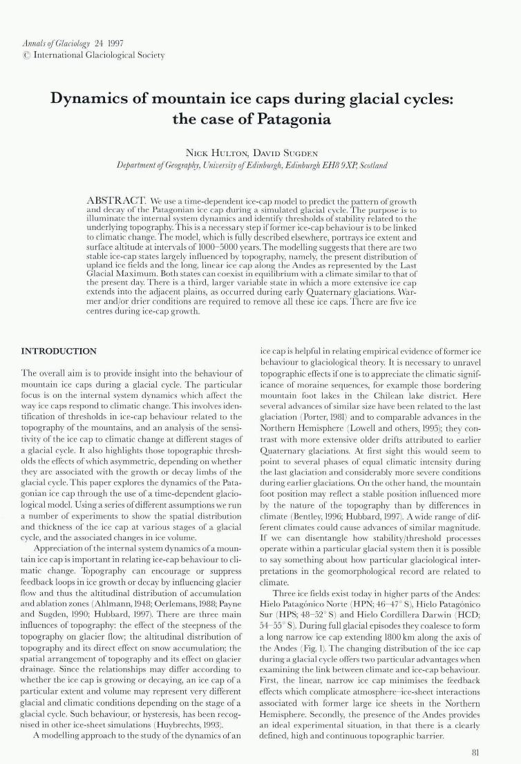
Three ice fi elds exist today in higher pa rts of the Andes: Hielo Pa tag6nico Norte (HPN; 46- 4r S), Hielo Patag6nico Sur (HPS; +8- 52° S) and Hielo Cordill era Da rwin (H CD; 54- 55° S). During full glac ia l episodes they coa lesce to form

a long na rrow ice cap extending 1800 km a long the axi s of the A ndes (Fig. 1). The cha nging di stribution of the ice cap during a glacial cycle offers two pa rticul a r advantages when exa mining the link between climate a nd ice-cap behaviour. First, the linear, na rrow ice cap minimises the feedback effects which complicate atmos phere- ice-sheet interactions

associated with former la rge ice sheets in the Northern Hemisphere. Secondly, the presence of the Andes provides an ideal ex perimenta l situation, in tha t there is a clea rly defin ed, high and continuous to pographic ba rri er.

81

H ulton and Sugden: Dy namics ojmollntain ice caps

• 45°

Rio Deseado

_ Lakes

50° ~ Icefields

Late Quaternary ice limits

Early-Middle Quaternary ice limits

55°

78° 76° 74° 72° 70° 68° 66° 64° 62°

Fig. 1. L imits of the Last Glacial Alaximum and early -Q,uatemmJ glaciations in Patagonia. After Cla/JjJerton (1993).

The Patagonian ice cap is in a clim atically signifi cant

location since it lies athwart the Southern H emisphere wes­terli es. At present, maximum precipitation at sea level is 6000- 8000 mm and occurs in la titudes 48- 52° S, fa lling to 2000 mm to the north and south (Mill er, 1976). Winds vary in both persistence and velocity in the same way; for exam­ple, at latitude 52° S the average daily wind speed is 12 m s- ', and velocities greater than 30 m S- I occur each month. M ean annual temperatures, with a low seasonal range typi­cal of a ma ritime clim ate, fa ll from 11.0°C at latitude 42° S to 5.5°C at 55° S. The Andes, with an average altitude 0[ 2000-2500 m, form a barrier to the westerlies. They introduce a sha rp precipitati on contras t between the excessively wet windward fl ank and the semi-arid eastern fl ank. The glacio­logica l implication of the climatic setting is that an ice cap building up over the mountains spans latitudinal climatic zones from cool temperate in the south to wa rm temperate in the north . Also, there is a rema rkably strong west- east g radient in the magnitude of the mass balance va rying from up to 8 m in the mariti me west to less tha n 0.2 m in the semi­a rid east.

THE MODEL AND EXPERIMENTAL DESIGN

The approach in this paper is to use a glaciologicalmodel to identify thresholds and stabiliti es in the modelled Ice-cap

82

system. ,,ye assume that the maj or modelled components of

the ys tem are good analogues of the real system. These a re:

The m ass-balance- a ltitude relati onship.

The regional topography.

The ice-sheet form .

The ice-mass fl ux.

We explore the modell ed system's tendency to achieve a stable state given an initi al morphology and continuous steady forcing. In the experiments the general character o[ the mass-balance rel ationship stays unchanged in spite of ice-sheet g rowth. This is a simplification which means that the method does not permit study of the possible ways in which different ice-cap ta tes may in themselves influence the mass-balance- a ltitude relationship.

The model has been desc ribed in deta il by Hulton a nd others (1994). It is time-dependent and forced by changing the mass-balance-altitude relati onship. It reli es on a verti­cally integrated, ice-mass continuity model solved over a finite-difference grid with a resolution of 20 km. In the origina l work (Hulton and others, 1994) the experiments were designed so that the model achieved an equilibrium extent compa rable to that of the known limits of the Last Glacia l M aximum. The match between the resulting best­fit model and reality was quite good, in that the overall di-

Hutton and Sugden: D.)'Iwmicsr!/mollntaill ice cajJS

2500

Present-day ELA (4321514)

2000 Minimal conditions to produce present-day ice distribution (4341504)

I 1500

Cl '0

~ « 1000

500

ELA needed for deglaciation from maximum (512)

o+-----_+------~----~----~------+_----_+------~~~~~--~---37 39 41 43 45 47 49 51 53 55

Latitude ( 0 South)

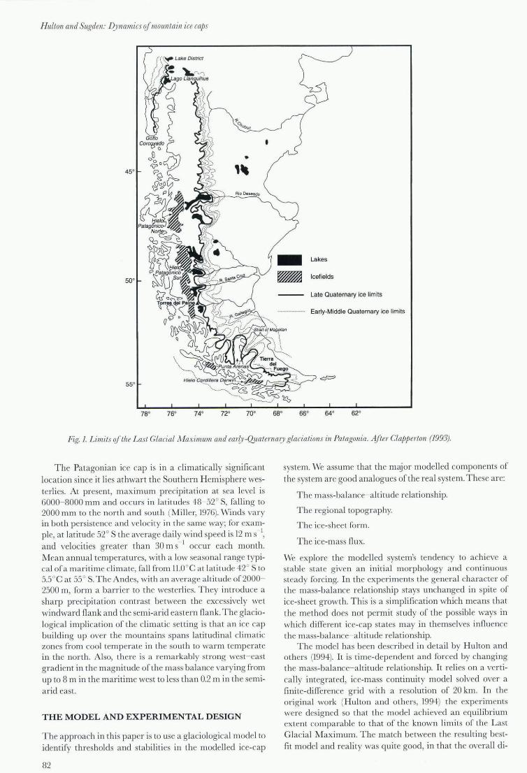
Fig. 2. Altitude of the jmsent-da.)1 ELA (after Hutton and others (1994)) and the ELAs used in this palm J!1 e include the ELA Jar the glacial maximum andJor various deglaciation scenarios. Numbers in jJarenlheses refer to particular model rUlls.

mensions of the ice cap and some of the la rger lobes were replicated in both . Sensitivity analyses showed that the

model was robust in its main conclusions. Changes in such factors as ice rheology had a modest effect on ice thickness but had littl e innuence on ice extent. R ather, the main con­clusion was that during the Last G lacial Maximum there was a differenti a l lowering of the equilibrium-line altitude (ELA) in different latitudes (a minimum lowering com­pared to the present of ",500 m at 40° S, ",100 m at 50° S a nd ",250 m a round 56° S) and a northwa rd migration of the westerli es which accentuated ELA lowering in the north a nd suppressed it in latitudes 46- 51 oS. The exp eriments in the present paper are based on the same model (Hulton and others, 1994). In the growth experiments the change in ELA was introd uced as a stepped function on an ice-free topo­graphy. Deglac iation was simulated by a stepped ELA ri se appli ed to ice maximum conditions. The absolute values and their denection from the present-day ELA a re shown in Figure 2. The values of ELA depress ion required to simulate glacial conditions vary from lat itude to lat itude, and range from 100 to 500 m. The lowering of the ELA a lso varies from west to east and renects the effect of continental­ity, as discussed elsewhere (Hulton and others, 1994). De­glac iat ion is simulated by a stepped return to present-day conditions. Also shown is the lowest possible ELA consistent with the present-day glacier extent. In one experiment we apply the latter ELA to the maximum ice extent during the Last Glacial Maximum.

These simple experiments a re sufficient to identify the main relati onships between topography a nd ice-cap beha­viour. But it is important to be aware of the key assumption. Forcing by a stepped change implies an instant mismatch with initi a l conditions, which in turn means that the effect of any non-linear relationship is emph asised more than if the rate of cha nge is g radual. For exampl e, the relationship between mass balance and altitude is non-linea r, in that the ablati on-dominated lower part of the curve is steeper than the higher-a ltitude part of the curve inOuenced mainl y by acc umul at ion. This means that a stepped change in mass­bala nce forcing will emphasise two effects. First, it wi ll result in a n unrea listically rapid response of the ice cap to change; secondl y, it will accentuate the asymmetry whereby

an ice cap responds more quick ly to warming (dominated by ablation at low a ltitudes) tha n cooling (dominated by

changes in acc umulation at higher a ltitudes ). It follows that in the experiments the use of model yea rs is only a g uide to the seq uence a nd relat ive length of the stages of growth and decay. Model years have littl e significance in absolute term s. There is a further, third implicat ion foll owing from the use ofa stepped change in the forcing function. It is that a rela­

tively small change might be amplified over time to create widely different stabl e states of the ice ca p. In the more com­plicated condi tions of the real world it is likely that the init­ia l change would have to be much larger to have the same effect. Thus the experiments indicate no more than the minimum changes in forcing required to move the ice cap

from one stable state to another. The model does not a llow for the effec ts of isostasy. Sen­

siti vity tests show that isostatic compensation plays a rela­ti vely subdued role in Patago ni a mainl y because the ice cap covers the mountain range onl y thin ly. This means that changes in ice thickness are sma ll in relation to changes in ice extent. The main effect of including isostatic compensa­tion beneath a growing ice mass is to slow down the build-up of ice and to accommodate greate r ice thicknesses, but with­out changing ice surface elevations. Since the latter are the ma in foc us of the experiments in thi s paper, the exclusion of isostasy is unlikely to affect the ma in conclusions.

DESCRIPTION OF MODEL RESULTS

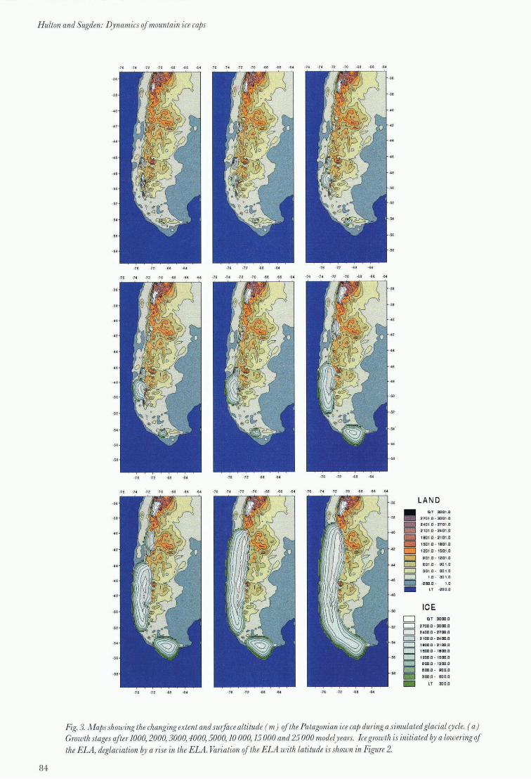
Figure 3 shows the extent and surface altitude of the ice cap during its growth and decay. The initi a l stages of growth are mapped at 1000 model-yea r intervals; the middle a nd later parts of the cycle are shown at longer intervals. Initi ally there a re five growth centres, the uplands of the existing ice fi elds and two centres in the north (Fig. 3a). Most growth is westwards towards the precipita ti on source. HPS grows fastest, and by 5000 model years it has reached the coas t and is contiguous with HPN. Ice then expands up and down the ax is of the Andes, mainl y on the western fl ank of the main cha in. Ice from the northern ice centre at 42° Sand ice from the southern centre ove r HCD both reach the coast

83

Hulton and Sugden: Dynamics ofmountain ice cajJs

84

-16 -12 -76 -72 -68 -64

-76 -74 -72 -70 -68 -66 -6 4 -16 -14 -72 -70 -68 -66 -64 -76 ·14 -72 -70 -68 -66 -64

· 76 ·72 ·68 ... ·76 ·72 ~. ... ·76 ·72 . " ... ·76 ·H ·72 ·70 ·68 ~. ~. ·76 ·72 ·70 ." . " ... ·76 ·H ·72 ·70 ~. ·86 ...

LAND GT 3001 .0

2701 n - 3001 .0

2401 D · 2701 .0

21[]1.o · 240 1.0

l lD l D · 2 101.0

l SD1.D ·1 BD 1.[1

12011] · 15 0 1.0

901.0· 120 1.0

B0 1.0 · 901.0

301.0 · 801.0

301.0

-250 .0 · I.. LT -250 .0

ICE D GT :1000 .0

D 27[][]D :1[] [][] .O

D 2400.0 2700 .0

CJ 2100.0 2400 .0

D I IDDD · 2100 .0

D 1500.0 · 1100 .0

D 1200.0 · 1500 ,0

D 1100 .0 - 1200 .0

D 800 .0 · BOO .D

300 ,0 - 800 .0 -LT lOD .D

·70 ·72 ." ... ·76 ·72 ·68 ." ·76 ·72 ·68 . ..

Fig. 3. il1aps showing the changing extent and surface altitude ( m) if the Patagonian ice cap during a simulated glacial cycle. ( a) Growth stages after 1000, 2000, 3000,4000, 5000, 10000, 15 000 and 25 000 modelyears. Ice growth is initiated by a lowering of the ELA, deglaciation by a rise in the ELA. Variation of the ELA with latitude is shown in Figure 2.

Hulton and Sugden: D)'namics ofmountain ice caps

-76 ·72 ·70 -68 -66 -6 4 -76 -74 -72 -70 -68 -66 -6 4 -76 -74 -72 70 -68 -66 -64

76 -72 -68 ." -76 -72 -S< 76

76 -72 -68 " -76 -72 -68

-H -7 0

LAND GT :JOD1.0

2701 D · :JO[]U]

240 1 D · 2701.0

2 101 D - 2401.0

11101.0 - 2101.0

15[]l D · li0 1.0

1201 D - 1S0 1.D

901.0 · 1201.0

SD I .D

301 .0 · BOI .!]

In - 30 1.0

·2SD .O · 1.0

LT -25 [] ,0

ICE GT 30[]O .O

HOOD · 30[]O .O

2400D - 27DIl .O

21[]OD ' 24 []O ,O

\ 1!IIlOD · llDO .a

lS00D - 1800.D

1l00D - ISOD .a

BDD ,D · 12DD,O

BOD .O· SOD .D

300 .[] - BOO .O

LT :mo.o

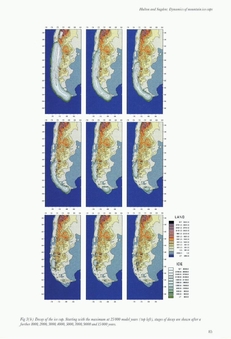
Fig 3( b) Deca), of the ice cap. Starting with the maximum at 25000 model )'ean (top left), stages of deca)' are shown after a further 1000,2000,3000,4000, 5000,7000, 9000 and 15 000 )'ean.

85

H ulton and Sugden: Dynanllcs rif mountain ice caps

900

800 /-100mELA

700

~ 600 0

><

E 500 ~

7 th"ow __ la_n_d_s_------IBest Fit Maximum

Q)

E 400 :::J (5 > Q)

300 E.

200

100 Separate mountain ice caps +25 m ELA

+100 m ELA

0

0 5 10 15 20 25 30 35 40

Model time from zero ice conditions (ka)

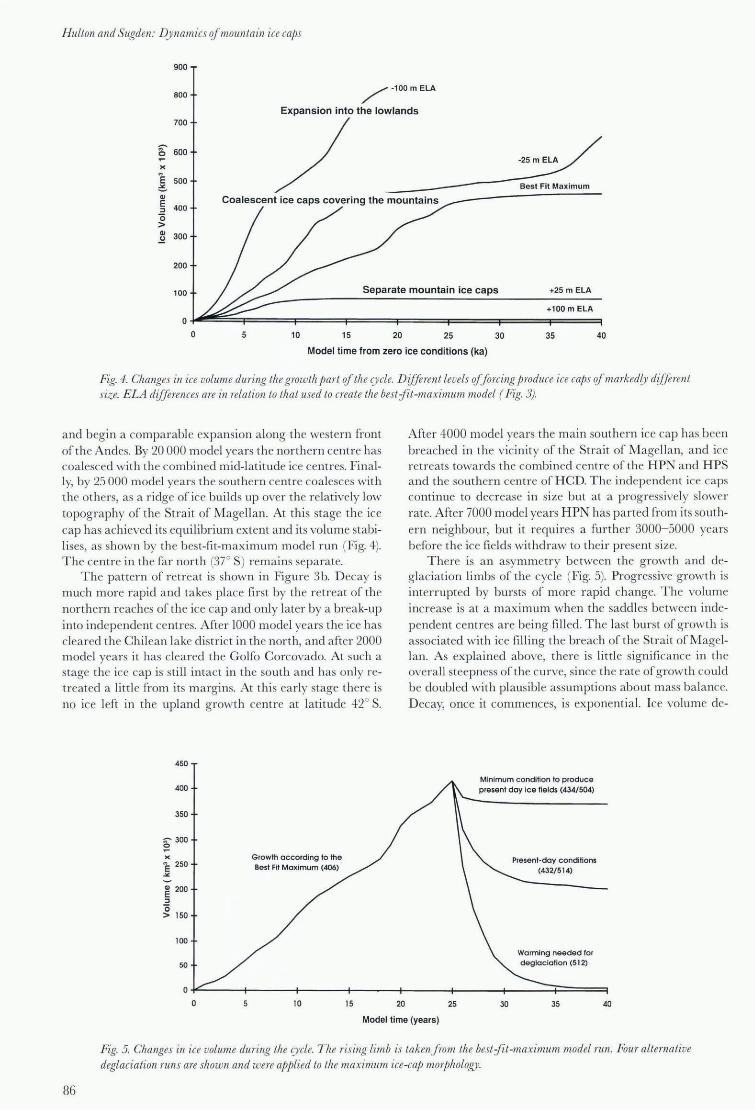
Fig. 4. Changes in ice volume during the growth part if the cycle. D ifferent levels if forcing produce ice caps if markedly different siz e. ELA differences are in relation to that used to create the bestjit-maximum model ( Fig. 3).

and begin a comparabl e expansion along the western front of the Andes. By 20 000 model years the northern centre has coalesced with the combined mid-latitude ice centres. Final­ly, by 25 000 model years the southern centre coa lesces with the others, as a ridge of ice builds up over the relatively low topography of the Stra it of M agellan. At this stage the ice cap has achieved its equilibrium extent and its volume stabi­li ses, as shown by the best-fi t-maximum model run (Fig. 4). The centre in the fa r north (37 0 S) remains separate.

The pattern of retreat is shown in Figure 3b. D ecay is much more rapid and takes place first by the retreat of the northern reaches of the ice cap and only later by a break-up into indep endent centres. A fte r 1000 model years the ice has cleared the Chilean lake district in the north, and a fter 2000 model years it has cleared the G olfo Corcovado. At such a stage the ice cap is still intact in the south and has only re­treated a little from its ma rgins. At thi s early stage there is no ice left in the upland growth centre at latitude 42° S.

450

400

350

M" 300 o

>< E 250 -"

E 200 :::J "0 > 150

100

50

Growth according to the Best Fit Maximum (406)

After 4000 model years the main southern ice cap has been breached in the vicinity of the Strait of M agellan, and ice retreats towards the combined centre of the HP)! and HPS and the southern centre of HCD. The independent ice caps continue to decrease in size but at a p rogress ively slower rate. After 7000 model years HPN has p a rted from its south­ern neighbour, but it requires a further 3000-5000 years before the ice fields withdraw to their present size.

There is an asymmetry between the g rowth and de­glaciation limbs of the cycle (Fig. 5). Progressive growth is interrupted by bursts of more rapid change. The volume increase is a t a m aximum when the saddles between inde­pendent centres a re being fill ed . The last burst of growth is associated with ice filling the breach of the Strait of M a gel­lan. As explained above, there is littl e signifi cance in the overall steepness of the curve, since the rate of growth could be doubled with plausible assumptions about m ass ba lance. D ecay, once it commences, is exponential. Ice volume de-

Minimum condition to produce present dav ice fields (434/504)

Present-day conditions (432/514)

Warming needed for deglaciation (512)

O~----~----_+----~~----+_----~----_+----~====~

86

o 10 15 20 25 30 35 40

Model time (years)

Fig. 5. Changes in ice volume during the cycle. T he rising limb is taken from the best fit -maximum model run. Four alternative

deglaciation runs are slzown and were applied to the maximum ice-cap morjJlzology.

HuLton and Sugden: l~Yllamics qfmolllztain ice caps

..

-76 72 ·68 -64 -76 72 -68 -64 -76 72 -68 -64

a b c -76 -74 -72 -68 -68 6' -76 -72 -10 -68 66 64

-72 -68 -64 -76 72 -68 -84

d e

LA N D GT 300 1.0

27D' [] lODLD

24010 2701.0

21010 2401.0

18010 2101.0

lSD1.D - lB01 .0

12D' 0 - 1S0 l.D

901 .0 - 1201.0

BOLD - 901.0

301 .0 - BOl.D

In - 301 .0

-2S0 .0 -

LT -250 .0

ICE CJ GT 3000 .0

c:=J 2700 Il· 3000 .D

c:=:J 21DD 0 - 2700 .0

2 100.0· 2400 .0

18000 2100 .0

1500D - l BOO .O

1200D - 1500 .0

900 .0 ' 1Z0D .a

BOD .a - 90D .O

300 .0- BOIl,[l

LT 300 .0

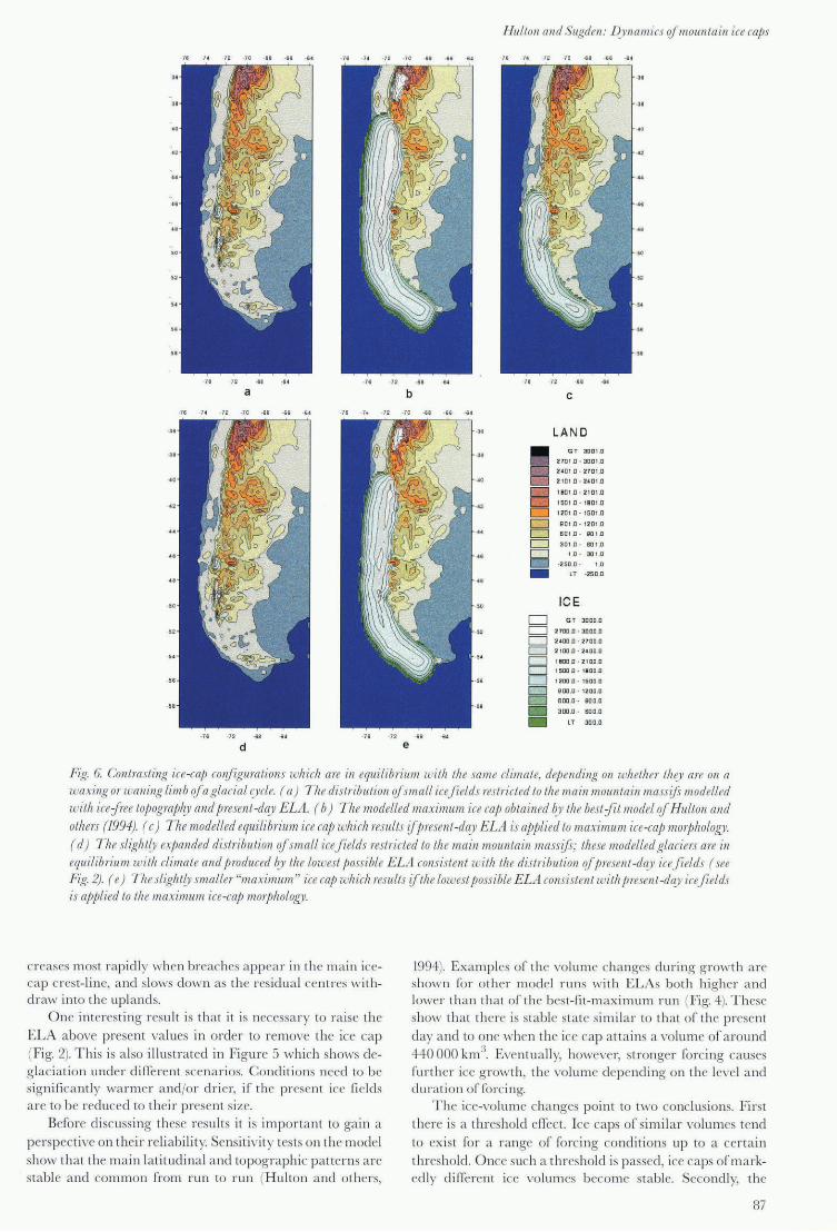
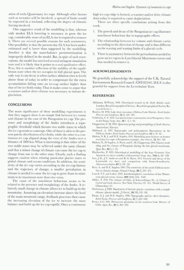
Fig. 6. Contmsting ice-call rO lyigumtions whim are in equilibrium with the same climate, de/lending on whether th~y are on a lOa ring or walling Limb qfaglaciaL c.vde. (a) The distribution qfslllalL iaJieLds restricted 10 the main mOllntain massifs modeLLed wiLh irefree Lopogmp/~y and presenL-day ELA. (b) The modeLLed maximum ire cap obLained ~v the besLfiL model qf H ulLon and others (1994). (c) The modeLLed equilibrillm ice cap which resuLts ifpresellt-do.v ELA is ap/)lied to ma rimum ire-caj) morphoLogy. (d) The sLightfy expanded distribution qfsmall ireJields restrlrted to the maillmollntain massifs; these modelled glaciers are in equilibrium with climate and produced ~Y the lowest possible ELA ronsistent with the distribution qf/)resellt-d{~y ireJields (see Fig. 2). (f) The sLightly smaLLer "maximum" ire cap which results if the Lowest flossibLe ELA consistent with presellt-d(~y irejieLds is af)plied to the maximum ice-rap morphology

creases most rapidly when breaches appear in the main ice­cap cres t-line, a nd slows down as the res idua l centres wit h­draw into the upl ands.

Onc interest ing res ult is that it is necessary to raise the ELA above present values in order to remove the ice cap (Fig. 2). This is a lso illustrated in Figure 5 which shows de­glac ia tion under different scenarios. Conditi ons need to be significantl y warmer and/or dri er, if the present ice fields a re to be reduced to their present size.

Before di scussing these result s it is important to gain a perspective on thei r reliability. Sensitivity tes ts on the model show that the main latitudinal a nd topographic patterns are stable a nd common from run to run (Hulton and others,

1994-). Examples of the volume changes during g rowth are shown for other model runs with ELAs both higher a nd lower th an that of the best-fit-max imum run (Fig. 4). These show that there is stable state simil a r to that of the present day and to onc when the ice cap attains a volume of a round 44-0000 km o. Eventually, however, stronger forcing causes further ice growth, the vo lume depending on the level a nd duration of forcing.

The ice-vo lume cha nges point to two conclusions. First there is a threshold effect. Ice caps of similar volumes tend

to ex ist for a range of forcing conditions up to a certain threshold. Once such a threshold is pas ed, ice caps of mark­ed ly different ice volumes become stable. Secondl y, the

87

Hutton and Sugden: Dynamics ofmountain ice caps

widely different responses to quite modest forcing show that the model is highl y sensitive to mass-ba la nce- a ltitude rela­tionships. This means that the model is suitable only for study of the structural relat ionships in the ice-cap system. Quantitat ive estimates such as those of timing and rates of growth and decay a re on ly indicative.

DISCUSSION

In spite of the relative simplici ty of the numerical model, the many assumptions needed to make it work and its obvious sensitivity to mass bala nce, it does contribute useful insights into some of the processes a ffecting the behaviour of the ice cap through a cycle of growth and decay. One implication of the runs in Figure 4 is that the modell ed ice cap reaches some so rt of equilibrium when it achieves a volume of

",440000 km :l. This occurs when the ice cap occupies its full latitudina l span along the mountain chain and Oows into the lowlands on either side. Once it is bounded by a ma rine cal­ving marg in in the west a nd subj ect to intense ablation in the relativel y warm lowland climates of the cast, it is diffi­cult for it to g row without much sha rper or longer forcin g.

Interestingly, this modell ed equilibrium state is very simil a r to the extent of the ice cap at the Last G lac ial Maximum (Fig. I). Also, the clustering of late-Quaternary mora ines at the mounta in front , as in the Chilean la ke di st rict, suggests that such a state occurred on several occas ions.

The implication of the match between model predictions

a nd empirical evidence is that there is a stable max imum state ach ieved by the Patagonian ice cap during glacial epi­sodes. The ma in reason seems to be the presence of a moun­tain range of sufficient altitude to acc umulate snow, bounded on each side by conditions which favour strong ab­

lation. A furth er implication of Fig ure 4 is that there a re two

eq uilibrium states for the ice sheet, sepa rated by a fin e cli­matic threshold. In onc, the best-Gt-m aximum run, the ice cap occupies its Last G lacial limits. In anoth e l~ with a low­ering of the ELA by only 25 m less, the ice remains in its current mountain centres. This implies that the topography of the mountain chain introduces a threshold; on one side of the threshold there a re glacial conditions similar to those of today; on the other there are full glacia l conditions. It is probabl e that the model represents the real-world situation and that the predicted beha\'iour is a response to the topo­graphy of the Andes. Under present conditions ice fi elds occur on di sc rete mounta in massifs ri sing above the ge neral level of the mountain cha in . A relatively modest lowering of the ELA brings much la rge r mountain co ll ecting areas into the acc umulation area a nd permits extensive build-up of ice. As the a ltitude of the ice surface ri ses there is a feedback effect which increases accumulation until the ice cap reaches its next stable position. This represents an effect long associated with upland a reas close to the glaciation limit (Ives and others, 1975).

Nonetheless it is important to add that in the case of the Patagonian ice cap the model is based on two key ass ump­tions and that these inOuence the clarity with which the two stable states a re distingui shed. The first ass umption is that the ice cap does not a lter the position of the ELA or the mass-ba lance Geld as it grows and decays. This is important to consider in the case of the large ice sheets that bui I t up in the Northern Hemisphere. H owever, the assumption seems

88

justifi ed in th e case ofPatagonia since the ice cap is na rrow, remains centred on the ax is of the Andes and has relatively li ttle effect on the overall a lti tude of the mounta in ba rri er as it g rows a nd decays. The main change to the mass-balance fi eld is an increase in the west- east mass-balance g radient (Hulton and Sugden, 1995). The second assumption is the stepped fo rcing which, as di scussed earli er, has the effect of accentuating any ice-cap res ponse. More gradual forcing over shon er time-scales wou ld reduce the sharpness of the threshold. But, even bearing such qua liGcations in mind , there seems no reason to doubt that the model points to a

di sti nctive tendency of ice-cap behaviour. Thus we concl ude that neither of the two ass umptions a ffects the main thrust of the a rgument, namely, that there is a threshold separat­ing two stable states which is a fun ction o f"th e topography.

This threshold has a different effec t on ice-cap stability dep ending on the direction of change, i. e. whether condi­

tions relate to the waxing or waning limb of a glacia l cycle. This means that an identical climate can produce a very dif­ferent ice-cap morphology, depending on whether the ice cap is bui lding up or decaying. This is illustrated by the ex­periments in Figure 6. In the first experiment the model is

run from an ice-free topography with the present-day ELA.

As expected, ice builds up in the locations presentl y occu­pied by HPN, HPS a nd HCD (Fig. 6a). Ice extent achieves a stable equilibrium with climate within 2000 model yea rs. When a n identical ELA field is applied to the max imum ice cap (Fig. 6b), the ice decays in the north but sta bili ses at

approximately halfits full glacial vo lume and survives as a large ice cap in the south a nd centre of its former domain (Fig. 6c ). The volume of ice remaining in equilibriu m with climate is vastly different in the two scena rios. Slart i ng with an ice-free topography, the equ ilibrium volume is onl y 20 X 103 km 3

. Sta rting with the maximum ice cap, the

volume stabilises at around 200 X 103 km 3

The second experiment is even more remarkable. H ere wc start with an ice- free topogra phy and apply the lowest poss ible ELA which is consistent with the existence and size of the present-day ice Gelds (Fig. 2). As before, equilibrium is achieved within 2000 model yea rs (Fig. 6d ). If thi s same ELA is a pplied to the maximum ice cap, there is only a min­or loss of volume and the full glacial ice cap is able to thrive in a climate which is only slightly wetter and/or cooler than today (Fig. 6e). In thi s case the contrast between the two equilibrium states is increased. The volumes are less than 50 X 10:l km 3 starting from a n ice-free topography, a nd about 360 x 103 km 3 sta rting with the maximum condi­tions. Again the two equilibrium states a re widely divergent a nd yet they coexist with identi cal climate but different starti ng conditions.

:Nloraines in the lowlands show that there are conditions under which the ice cap can extend beyond the mountain rea lm (Fig. 1). These show that ice extended over the eastern plains of Patagonia as fa r as the Atlanti c (Caldenius, 1932; Clapperton, 1993) and into the western lowlands in the northern lake di strict ( Porter, 1981). Presumabl y, such ex­pansion requires either stronger or longer forcing or a com­bination of the two. Ice ex tent will be a trade-off between acc umulation at higher a ltitudes on the ice surface and ab­lation in the lowland. The longer and more severe the for­cing, the g reater the ice extent will be. The experiments in Figure 4 suggest that the extra forcing required, compared to the best-Gt-maximum ru n, is equival ent to a lowering of the ELA by a furth er ",100 m. Perhaps thi s could be a simul-

a tion of ea rly-Quaternar y ice caps. Although other factors such as tecto nics will be invo lved, a spread of limits wo uld be expected in a lowland, relT ecting the degree of climatic forcing involved.

One suggestive result of the modelling is that, whereas onl y modest ELA lowering is necessary to g row the ice cap, considerably more of a n ELA rise is required to remove it. There are several possible reasons fo r such asym mctry. One poss ibilit y is that the present-day ELA has been under­estim ated and is lower than suggested by the modelling. Another is that the mass-balance parameteri zation is

improperly defined in the model. But, in spite of such rese r­vat ions, the model has survived several st ringent simulation tests a nd it is likely that it points to a rea l qua litati'T e/TeCl. If so, thi s is another relT ect ion of the stability of the equili­brium state when the ice occ upi es its full g lac ia l span. The onl y way it can decay is when surface ablat ion ri ses to levels

above those of today in order to compensate for the ext ra

acc umul at ion falling onto an ice-cap surface higher tha n that of the ice fi elds today. Thus it ma kes sense to arg ue th at a warmer and/or drier clim ate was necessary to initiate de­g laciati on.

CONCLUSIONS

The ma in sign ificance or these modelling experiments IS

that they sugges t there is no simple link between ice ex tent and clim ate in the case of the Patagoni an ice cap. The pre­sence a nd morphology of the Andes introduces a topo­

graphic threshold which fa, ·ours two stable states to which the ice cap tends to converge. One of these is akin to the pre­sent patc hy distribution of ice field s, whil e the other is a con­tinuous ice cap a ligned along the crest of the Andes over a di stance of 1800 km. What is interesting is that either of the two stable states may be achi eved under the same climate

a nd that a minor change of climate can cause the ice cap to change from onc to the other state. Clearl y, such a findin g suggests cauti on when relating particul ar glacie r states to g loba l climate a nd ocean conditions. In addition, the sensi­ti vity of the ice cap vari es acco rding to the ice-cap history and the traj ectory of change; a sma ll er pertubation in climate is needed to cause the ice cap to grow from its mini­mum to it s max imum state than vice versa.

The cause of the non-linear behaviour seems to be related to th e presence and morphology of th e Andes. A re­latively small change in clim ate a llows ice to build up in the

mounta ins. Assuming an el evation increase above the leve l of the ma in mountai n range, feedback processes then cause the increas ing elevation of the ice to increase the mass balance and build up the ice cap rapidly. Once a continuous

Hullon and Sugden: p.l'llamirs ofmountain ice caps

high ice-cap ridge is formed, a warmer a nd/or dri er climate than today is required to cause deglacia tion.

There are three specific conc lusions arising from thi s work:

I. The growth and decay of the Patagonian ice cap illustrates non-linea r behaviour due to topographic effects.

2. The relat ionship between ice vo lume and clim ate va ries acco rding to the di rect ion of change and is thus different on the wax ing and waning limbs of a glac ia l cycle.

3. There is asymmetry between the perturba tion needed to

g row an ice cap to its Last Glacia l M ax imum extent and t hat needed to remove it.

ACK NOWLEDGEMENT S

We g ratefull y acknowledge the support of the U K. Natural

Environment Research Council (GSTj02/544). nE.s. is also grateful for support from the Leve rhulme lhlst.

REFERENCES

Ahlmann, H. W:son. 19+8. Giacioiogirai rmarc/t on Ihr . forlh Allanli!" roasts. London, Royal Geograp hica l Sociely. (Roya l Geogra phica l Societ), Re­sea reh Series I.}

Ben tl ey. 1\1. 1996. Lake shore moraines. C hilean La ke District. Ea rlh Slnjhre Processes and L(II/(Iforlll', 21 (Gi, 193 507.

Calden ius, C. C. 19:12. Las glaciaciones c lIat ern aria s en la Palagon ia y T ier­ra del FlIcgo. Grogr AIIII., 14 (I 2), 1-6+.

Clappcnon, C. i\ \. 1993. Qjlatrrllar)'ge%g)' and gfolllor/Jh%gJ' q/Sollth Allleriw. Amsterdam, Elsc, ·ier.

Hubbard, A. 1997. ' Io pography a nd palacoglae ier flu ctuat ions in th e Chile-an Andes. Earlh SurfilCf ProcessesalJd l.alJrlfonlJs 22 (1 }. 79 92 ..

Hullon, N. R.J. a nd D. E. SlIgdcn. 1995. ;'\Iodcll ing mass ba lance on lo n ner maritime ice ca ps: a Patagonia n example. AIIII. (aario/'. 21,30+ 310.

Hul lon, N., D. Sugden, A. Pay nc and C. I'd . C lappenon. 199+. G lacier mod­

cli ng and Ihe climale 0 (" Patagon ia during Ihe last g lac ial ma ximum.

OJwt. RI'S., 42 I , I 19. HuybrcclllS. P. 1993. G laciologica l modell ing of the Latc Ccnozoic Eas t

Antarctic ice sheet: stabilit y of dynamism? (;eogr AIIII .. 75A (+), 221 238. Iws, J. D., .J.T. Andrews a nd R. G. Barr)". 1975. Growt h and deca)' o f" the

La urentidc irr sheet and cOInparison wit h Fcnno-Scandinav ia. Xalurz";ssfllsc!w!len. 62 (3, 11 8 125.

Kerr, A. and D. E. Sugden. 199~. The sensili , ·ity of the sO lllh Chilean snow­

line to clim ale cha nge. Climatir Change, 28 (3), 255 272. Lowcll , T.\~ and 8 others. 1995. Interhemispheric correlat ion o /" late Plcisto­

cene g lac ial evcnts. Science, 269 (5230), 15+1 15+9. J\li I Ier, A. 1<J76. The climate of Ch ile. I II Schwerdtfeger, W. , ed. Climales of

Celllml alld Soulh . lmerira. i'\cw York, El sc, ·ier, 113 1+5. (World Surve)" o/" C li mato logy 12.)

O erl cma ns, J. 1988. Simul at ion of" hi storic g lacier var ia tions wil h a simple

c1imal e-glacier mocJe\. J (;ia rio/., 34 (118), 333 3+1. Payne, A. J. a nd D. E. Sugdcn. 1990. Topography a nd ice sheet dynamics.

I,·arth Surfare Processes alld Lalldforms, 15 (7}, G25 639. Pon er, S. C. 1981. Plr istocene g lacia ti on in the southern Lake Distric t of

C hil e. QJlal. Res., 16 (3}, 263 292.

89