THESIS FOR THE DEGREE OF LICENTIATE OF ENGINEERING

Dynamics of large-scale fluidized bed combustion plants

Modeling, simulation and control

GUILLERMO MARTINEZ CASTILLA

Department of Space, Earth and Environment

CHALMERS UNIVERSITY OF TECHNOLOGY

Gothenburg, Sweden 2021

Dynamics of large-scale fluidized bed combustion plants

Modeling, simulation and control

GUILLERMO MARTINEZ CASTILLA

© GUILLERMO MARTINEZ CASTILLA, 2021.

Department of Space, Earth and Environment

Chalmers University of Technology

SE-412 96 Gothenburg

Sweden

Telephone +46(0)31-772 1000

Printed by Chalmers Reproservice

Gothenburg, Sweden 2021

i

Dynamics of large-scale fluidized bed combustion plants Modeling, simulation and control

GUILLERMO MARTINEZ CASTILLA Division of Energy Technology

Department of Space, Earth and Environment

Chalmers University of Technology

Abstract

Fluidized bed combustion (FBC) plants are widely used in energy systems across the world for

the thermochemical conversion of solid fuels, and are especially suitable for low-rank fuels (a

category to which renewable solid fuels belong). FBC plants are traditionally operated for base-

load electricity production and for heat production, both of which processes are characterized

by steady and stable operation. As the share of variable renewable electricity (VRE) sources is

expected to increase dramatically, FBC plants will have to adapt their operations to the new

flexibility requirements related to the inherent variability of VRE sources. By enhancing their

operational and product flexibilities, FBC plants can remain financially attractive and offer

services to support the balancing of the grid. As tools for assessing the operational flexibility

of thermal power plants, dynamic modeling and simulation are gaining attention from both

researchers and plant operators. However, it is a common practice to assume that the dynamics

of the gas side are much faster than those of the water-steam side, i.e., not accounting for the

in-furnace dynamic mechanisms.

This thesis aims to characterize the dynamic behaviors of commercial-scale FBC plants,

accounting for both the gas and water-steam sides of bubbling and circulating fluidized bed

(BFB and CFB) units. For this purpose, a dynamic semiempirical model of the gas side of FBC

plants is developed and integrated into a process model of the water-steam side. The models

are validated against steady-state and transient operational data measured at two commercial-

scale industrial units. The model is then used to analyze the inherent dynamics of the gas and

water-steam sides, to compare the transient behaviors of BFB and CFB units, and to assess the

dynamic performances of FBC plants when operated under different control structures.

The results of the dynamic analysis show that the stabilization times of the temperatures across

the furnace differ, largely based on the local heat capacity of the region in the furnace, i.e., the

amount of bulk solids. The work includes an assessment of the impact of the characteristic

times of the in-furnace mechanisms (i.e., fluid dynamics, fuel conversion and heat transfer) on

the computed stabilization times of key in-furnace variables at plant level, and suggests some

simple mathematical relationships for predicting these times. When accounting for the water-

steam side, the results show that the inherent dynamics of variables such as live steam pressure,

flow and power production are in the same order of magnitude as the dynamics of the gas side,

particularly for the CFB case. This highlights the importance of accounting for the gas side

when attempting to model accurately the dynamics of FBC plants. Furthermore, FBC plants

are found to be able to provide fast load changes when operated under control structures that

manipulate the live steam valve, although this is found to trigger operational issues, such as

pressure overshoots.

The results of this thesis are of particular importance in terms of assessing the transient

capabilities of FBC plants to operate in electricity-driven markets where fast operation is

ii

required, and they can be used to identify opportunities and challenges. Furthermore,

knowledge about the transient operation of large-scale FB reactors will be crucial for the

development of FB applications other than combustion, such as polygeneration or

thermochemical energy storage.

Keywords: operational flexibility, thermal power plant, process control, combined heat and

power, biomass combustion

iii

List of publications

The thesis is based on the following appended papers, which are referred to in the text by their

assigned Roman numerals:

I. G.M.Castilla, R.M. Montañés, D. Pallarès and F. Johnsson.

“Dynamic modeling of the reactive side in large-scale fluidized bed boilers”.

Industrial and Engineering Chemistry Research, 2021, 60, 3936-3956.

II. G.M.Castilla, R.M. Montañés, D. Pallarès and F. Johnsson.

“Comparison of the transient behaviours of bubbling and circulating fluidized bed

combustors”.

Submitted for publication, 2021

III. G.M.Castilla, R.M. Montañés, D. Pallarès and F. Johnsson

“Transient operation capabilities of biomass-fired fluidized bed combined heat and

power plants. Dynamic modeling and control”.

To be submitted, 2021

Guillermo Martinez Castilla is the principal author of Papers I – III and performed the

modelling and analysis for all three papers. Rubén M. Montañés contributed to the method

development in Papers I-III as well as with editing and discussion for all three papers.

Associate Professor David Pallarès contributed to the method development in Papers I-III, as

well as with editing and discussion for all three papers. Professor Filip Johnsson contributed

with discussion and editing in Papers I-III.

iv

Other publications by the author, not included in the thesis:

• G. M. Castilla, M. Biermann, R.M. Montañés, F. Normann and F. Johnsson.

“Integrating carbon capture into an industrial combined-heat-and-power plant:

performance with hourly and seasonal load changes”.

International Journal of Greenhouse Gas Control, 2019, 82, 192-203.

• G. M. Castilla, A. Larsson, L. Lundberg, F. Johnsson and D. Pallarès.

“A novel experimental method for determining lateral mixing of solids in fluidized

beds – Quantification of the splash-zone contribution”.

Powder Technology, 2020, 370, 96-103.

• G. M. Castilla, D.C. Guío-Pérez, S. Papadokonstantakis, D. Pallarès and F. Johnsson.

“Techno-economic assessment of calcium looping for thermochemical energy storage

with CO2 capture”.

Energies, 2021, 14, 3211

• G. M. Castilla, R.M. Montañés, D. Pallarès and F. Johnsson.

“Dynamic modeling of the flue gas side of large-scale circulating fluidized bed

boilers”.

In proceedings of CFB-13 conference, Vancouver, Canada, 2021

v

Acknowledgements

I would like to start by thanking my supervisors: each of them has been a key piece for the

development of this work. Working with 4 supervisors is a continuous learning for which I am

thankful every single day. First of all, David, thank you for being a steady light glowing through

the dark winters. Not only your knowledge and dedication are precious, I also truly appreciate

our abundant non-work conversations, from music and sports to travelling and literature.

Rubén, infinite thanks for your support, hours-long discussions, brainstorming, inspiration and

many more. It has been now more than three years working back to back, and only you know

how important your presence is for me, and for this work. Filip, thank you for always finding

the time and energy to bring up new ideas, perspectives, and discussions. Your time

management is something that truly fascinates me and learning from you is very inspiring. Last

but not least, thank you Carolina for moving to Gothenburg in the middle of a global pandemic

and joining the team. In only one year I have already learnt lots from you and I can´t wait for

all the discussions ahead of us!

My gratitude goes also to my examiner Henrik Thunman, whose busy office has always been

open for me. Very special thanks to Fredrik, Max and Stavros for opening me the doors of the

division three and a half years ago and initiating this longer-than-expected adventure.

Thank you Bioshare for a great collaboration and useful discussions, all the luck for all the

exciting projects you have ahead! Thanks also to Karlstad and Övik Energi for an impressive

work answering to all our requests.

Co-workers of Energy Technology: thanks to all of you for contributing to create the fantastic

workplace we have. With this regard, special mention to Marie and Katarina for their

everlasting good and helping mood we all should learn from. Thanks to my PhD colleagues

(some of you now friends) for lunches, walks, afterwork sessions, board games, volleyball and

more. Sharing this adventure with you all is crucial for me. Special thanks also to my office

mate Tove: I wish you all the best in the future! To the newly born Fluidization group, thanks

for our Monday meetings and the space for sharing and discussing that we have created in this

short time.

I would not be the person I am without my friends. Thank you Guarida for that. Also big thanks

to my friends in Gothenburg and Iceland for being my family far from home

Lastly, I would like to thank my family for making all this possible. I can feel your love and

support no matter where we are. Stef, it is a real joy to walk next to you day after day, alltaf.

Thanks for continuously teaching me about the things that really matter in life.

This work has been financed by the Swedish Energy Agency under the project “Cost-effective

and flexible polygeneration units for maximized plant use” (P-46459-1).

Guillermo Martinez,

Majorna, May 2021

vi

vii

“If we take care of the moments, the years will take care of themselves”

- Maria Edgeworth

viii

ix

Table of Contents

1. Introduction ..................................................................................................................................... 1

1.1. Aims and scope ....................................................................................................................... 3

1.2. Outline of the thesis ................................................................................................................ 3

2. Background and related work ......................................................................................................... 7

2.1. Power plant flexibility ............................................................................................................. 7

2.2. Fluidized bed combustion ....................................................................................................... 8

2.2. Dynamic modeling of FB boilers ............................................................................................ 9

3. Methods......................................................................................................................................... 13

3.1. Reference units ...................................................................................................................... 13

3.2. Modeling and simulation ...................................................................................................... 16

3.3. Dynamic analyses ................................................................................................................. 17

4. Dynamic model ............................................................................................................................. 23

4.1. Gas side ................................................................................................................................. 24

4.2. Water-steam side ................................................................................................................... 27

4.3. Model calibration and validation .......................................................................................... 28

5. Selected results and discussion ..................................................................................................... 33

5.1. Inherent dynamics of FBC plants .......................................................................................... 33

5.2. Controlled dynamics ............................................................................................................. 38

5.3. Dynamic interaction between the gas and water-steam sides ............................................... 40

6. Conclusions ................................................................................................................................... 43

6.1. Further work .......................................................................................................................... 44

References ............................................................................................................................................. 45

x

xi

Nomenclature and terminology

Latin symbols

A: area

a: decay factor

C: controller

c: concentration, heat capacity

D: diameter

F: flow,

h: heat transfer coefficient

I: instrument

K: transport decay factor, backflow effect ratio, flow area coefficient

k: decay constant, absorption coefficient

L: level, lenght

M: total mass

P: pressure instrument

p: pressure

Q: heat flow, composition,

R: reading

St: stokes number

T: temperature, transmitter,

t: time

u: velocity

y: process variable

Greek symbols

τ: characteristic time

η: efficiency

ε: voidage

σ: Stefan-Boltzmann constant

ρ: density

Subscripts

b: backflow

c: convection, core

comb: combustion

db: dense bed

DH, in: inlet district heating water

DH, out: outlet district heating water

e: equivalent

el: electricity

entr: entrained

extracted, i: extracted in a certain cell i

f: fuel

g: gas

xii

in: inlet

n: nominal

p: particle, at constant pressure

rad: radiation

s: stabilization

susp: gas-solid suspension

t: terminal, turbine

top: at furnace top

vol: volumetric

w: wall

Walls: to the waterwalls

wl: wall-layer

0: before change is introduced

∞: after new steady-state is reached

Abbreviations

BF: boiler-following

BFB: bubbling fluidized bed

CFB: circulating fluidized bed

CHP: combined heat and power

CP: centrifugal pump

DH: district heating

DHC: district heating condenser

DSH: desuperheater

ECO: economizer

FB: fluidized bed

FBC: fluidized bed combustion / combustor

FC: fuel conversion

FD: fluid dynamics

FG: flue gas

FP: floating pressure

FWH: feedwater heater

HHV: high heating value

HPT: high pressure turbine

HT: heat transfer

IPCD: integrated process control design

IPT: intermedium pressure turbine

LPT: low pressure turbine

MPC: model predictive control

OFWH: open feedwater heater

RC: relative change

SH: superheater

SP: set-point

TF: turbine-following

VRE: variable renewable electricity

VRR: variable ramping rate

TCES: thermochemical energy storage

xiii

Glossary

The following terms are recurrent throughout the text:

Controlled dynamics: Transient behavior of the plant/furnace when running with

closed (i.e. activated) control loops.

Dynamic analysis: investigation of the different aspects related to the transient

operation of FBC plants.

Gas side: Combustion chamber of the furnace in which the fuel, bulk solids and gas are

located. In some contexts, also referred as in-furnace. Note that the furnace walls and

convective flue gas path are in this work considered part of the water-steam side.

Inherent dynamics: Transient behavior of the plant/furnace when running with open

(i.e. deactivated) control loops.

Model calibration: Fine-tuning of model parameters to adjust the model output so that

it resembles more accurately a specified operational dataset of a certain reference unit.

Model formulation: Writing and balancing of the model, i.e. of the system of equations

consisting of mass and heat balances.

Model validation: Use of the calibrated model to predict steady-state and transient

operational datasets others than the one used for calibration.

Open-loop: Uncontrolled response of the system variables after a step-change in one of

the inputs.

Reference units: Commercial-scale FBC plants used for collecting operational data.

Water-steam side: All the equipment related to the water-steam loop conforming the

Rankine cycle, i.e., the convective flue gas path (economizers and superheaters),

evaporator tubes and in-furnace walls, steam drum, steam lines and valves, steam

turbines, condensers, deaerators, feedwater heaters, pumps and valves.

1

1. Introduction

In accordance with the Paris Agreement [1], decarbonization of the power sector is a priority

to maintain global warming at well below 2°C above pre-industrial levels [2]. Electricity supply

from renewable sources such as wind and solar represents a key solution to this challenge [3],

and the share of renewable sources in the worldwide electricity generation is expected to

increase from 25% in Year 2016 to 33% in Year 2025 on global level, playing a crucial role by

Year 2050 in the electricity production of most European countries [4],[5]. However, electricity

generated from wind and solar power is subject to weather variations, so it is often referred to

as variable renewable electricity (VRE). This intermittency creates a need for power system

balancing to ensure security of supply at all times. As the share of VRE generation surges, the

variations in the net load curve (calculated by subtracting the renewable energy generation

from the total energy demand) increase. This net load is currently met by thermal power plants

in most of the energy systems worldwide [6], and the impact of the penetration of VRE on the

operational patterns of these plants is already noticeable in some regions [7], as they are

operated to provide regulation and back-up capacity to the grid during periods with very low

levels of solar and wind power generation [8]. Thus, it is clear that practically all thermal power

plants existing and to be commissioned for power production will be required to adapt their

operation to the fluctuating market conditions created by the high-level penetration of VRE.

The term ‘flexibility’ is currently used widely, and it is therefore important to establish

definitions depending on the context and the timescales. A recent paper from Beiron et al. [9]

has defined different types of flexibility, categorized according to plant-level (operational and

product flexibility) and system-level flexibilities (thermal, electricity system, fuel supply and

climate flexibilities). Operational flexibility is defined in that study [9] as the ability of a plant

to vary its output by adjusting the input thermal load from the fuel conversion system. Among

the different types of thermal power plants, solid-fuel boilers are the slowest in the operational

flexibility spectrum (see [8][10]), especially those that burn low-grade fuels (to which

renewable solid fuels typically pertain) such as biomass and waste. For the conversion of these

fuels, fluidized bed combustors (FBCs) are the preferred technological choice due to the strong

mixing and heat transfer capabilities offered. Thus, FBC plants play a crucial role in many

energy systems around the world [11][12], and their operation is directly affected by the need

for increased operational flexibility stated above. Yet, the vast majority of FBC plant setups

are either: (i) larger coal-fired units for base-load electricity generation; or (ii) smaller

biomass-fired or waste-fired units for combined heat and power (CHP) generation, with heat

as the main output governing the plant dispatchability [11]. Moreover, the two existing types

of FBC units, bubbling and circulating fluidized beds (BFB and CFB, respectively, with the

latter having larger specific thermal capacity and typically larger sizes), have a large in-furnace

solids inventory that yields plant systems that are characterized by delay, strong coupling

among parameters and non-linear behaviors [13]. Thus, conventional operation of FBC units

is characterized by small and slow load changes compared to other solid fuel combustion

alternatives, such as pulverized coal plants [14], and the limits related to the transient

capabilities of FBC units remain largely unexplored.

The importance of mastering the dynamic operation of FBC plants has been highlighted by

several authors [15][16]. Investigations of the transient performances of effective control and

2

operational strategies would enable current FBC setups to increase their participation in various

electricity markets, expand their product portfolio and, thus, remain financially attractive.

Furthermore, large-scale FB reactors are at the core of several novel energy processes in early

developmental phases in which the transient performance is foreseen as being crucial. Two

major examples of these developments are: i) the retrofit of FBC plants into polygeneration

facilities in which output energy vectors other than heat and power (e.g., fuel gas, char,

hydrogen) are produced [17], [18]; and ii) thermochemical energy storage through solids

cycling [19], [20], [21]. There are two main constraints that currently limit the introduction of

flexibility into FBC plants in terms of load ramping. First, due to the complexity of the

fluidization phenomena and the relatively large lack of industrial measurements, the inherent

dynamics of FB boilers are still largely unknown, which means that fast ramping is a non-

optimized process for most units, which may entail undesired consequences such as high

emission levels [22]. Second, cyclic operation implies increasing stresses on plant components,

and this results in reductions in equipment lifetimes and increased operational costs [23], [22].

Dynamic process modeling is gaining attention as a tool that can provide insights into the

transient behaviors of power plants, as it allows operators and plant owners to evaluate various

operational and control strategies that can lead to increased profits in the present and future

energy markets [24], [25]. However, this strategy relies heavily on the reliability levels of the

models used. While unit-specific models for conventional operation of existing furnaces and

plants can be developed based on correlations derived from site measurements, general model

formulations with a more solid theoretical ground are needed to study unit designs, sizes and

operations outside the scope covered by site measurements. In particular for FB combustors,

low-order, semiempirical models represent an optimal trade-off between accuracy, generic

applicability, and low computational cost to be integrated into dynamic process models [26].

Alobaid et al. [25] have published an extensive review of dynamic modeling and simulation of

thermal power plants, including a wide range of technologies and feedstocks, from which the

following points can be extracted: i) there is a lack of dynamic modeling studies that focus on

biomass-fired plants; and ii) there is very limited knowledge about the dynamic behaviors of

FB boilers. Similar conclusions can be drawn from the recent review of Avagianos et al. [27],

which is dedicated to dynamic modeling and simulation of solid-fuel power plants: there is a

clear deficit of dynamic models that include FBCs, as well as of dynamic models of large-scale,

biomass-fired units. Lastly, Atsonios et al. [15] have reviewed the existing dynamic process

models of bio-based heat and power plants, highlighting the scarcity of such models as

compared to models of fossil-fueled plants. Among the few published dynamic modeling

investigations of biomass-fired power plants, the review highlights the scarcity of studies that

account for the flue gas side of FB combustors, especially those that have been validated with

site measurement data.

In summary, there is a growing need for FBC plants to increase their operational and product

flexibility levels, in order to adapt to the new requirements associated with energy systems that

have a high penetration of VRE. Due to the complexity of the fluidization phenomena, the lack

of measurements from industrial-sized units, and the traditional steady operation of these

plants, there is a knowledge gap regarding the transient capabilities of FBC plants. Although

dynamic power plant modeling is a widely used tool to characterize and study the transient

performance of power plants, very little work has been performed on the inherent and

3

controlled operational capabilities of FBC plants through thorough dynamic descriptions of

both the gas and water-steam sides.

1.1.Aims and scope

The overall aim of this thesis is to characterize the dynamic behavior of large-scale FBC plants,

so as to facilitate their transition into the forthcoming energy systems with high penetration

levels of VRE. The scope of the work includes both the gas and the water-steam sides of

commercial-scale FBC plants for combined heat and power production.

More specifically, this thesis attempts to fill the two major knowledge gaps by addressing the

following research questions:

i) What are the inherent dynamics of FBC plants associated with load and fuel

changes?

ii) How can control and operational strategies improve the operational flexibility of

FBC plants?

To answer these questions, the present work makes use of semiempirical dynamic modeling to

describe the transient performances of the reactor and water-steam process equipment of FBC

plants. The specific objectives of the thesis are the following:

1) To develop a model that is capable of describing the dynamic behaviors of industrial-

scale FBC plants while accounting for both the gas and water-steam sides.

2) To analyze the inherent dynamics of large-scale FBC plants when the load, fuel

composition and district heating (DH) production level are varied.

3) To characterize the in-furnace mechanisms driving the inherent dynamics of FBCs.

4) To compare the dynamic behaviors of BFB and CFB combustors.

5) To evaluate the operational capabilities of FBC-CHP plants to provide fast load changes

when operated under different control structures.

6) To assess the interplay between the dynamic responses of the gas and the water-steam

sides.

1.2. Outline of the thesis

The present thesis comprises a summary dissertation and three appended papers. The

dissertation consists of six chapters, for which the linkages with the three appended papers

(Papers I–III) and the performed activities are depicted in Figure 1. After the introductory

Chapter 1, Chapter 2 provides the background of the work and a literature review of the

dynamic modeling assessments previously carried out for FBC plants. Chapter 3 presents the

methods used in the work, Chapter 4 describes the formulation, calibration and validation of

the dynamic models, Chapter 5 highlights and discusses the main findings of the work, and

Chapter 6 concludes the thesis in relation to the aims, research questions and objectives set,

and incorporates a brief discussion on future work.

4

As shown in Figure 1, the model of the gas side is capable of describing both BFB and CFB

combustors; and an FBC-CHP plant model has been developed from integrating the gas side

model into a dynamic process model of the water-steam side. Operational data from two

reference units are used for the calibration and validation of the dynamic models. Lastly, the

furnace and plant models are used for carrying out various dynamic analyses of the gas and

water-steam sides of CFB and BFB units, including examinations of control and operational

strategies imported from the literature. The findings of this thesis are of relevance to various

thermochemical processes where large-scale FB reactors are expected to operate dynamically,

as further discussed in Chapter 6.

Figure 1. Schematic of the thesis structure. Light green area: Modeling and simulation activities. Dark blue

boxes: non-modeling activities. Yellow boxes: scope within FBC plants. Grey boxes: outputs from the analyses.

Light blue: appended papers.

Paper I presents a dynamic model of the gas side of large-scale FBC plants. The model, which

is capable of describing both BFB and CFB furnaces, is validated against operational data from

one reference unit of each type. After the formulation, calibration and validation of the model,

the paper focuses on studying the partial load performances of the reference units prior to the

analysis of the inherent dynamic behavior of the gas side when the load and fuel composition

are changed.

Paper II uses the gas side model presented in Paper I to compare the transient performances

of BFB and CFB furnaces after eliminating the thermal size effects (given that two units of the

same size, 130 MWth, are simulated). Furthermore, the paper investigates the impacts of the

characteristic times for each of the dominant in-furnace mechanisms (fluid dynamics, fuel

conversion, heat transfer) on the stabilization times of the furnace temperatures and heat

extraction in BFBs and CFBs.

Paper III investigates the transient capabilities of CFB-CHP plants, including both the gas and

the water/steam sides. The gas-side model presented in Paper I is integrated into a dynamic

5

process model of the water-steam side, and the resulting integrated FBC plant model is

validated against steady-state and transient operational process data obtained from an industrial

CFB-CHP plant. The paper includes a comprehensive review of the main control strategies for

load changes applicable to CFB-CHP plants. Finally, the paper studies the interactions between

the inputs (e.g., fuel and air flows) and outputs (e.g., power and heat production) of the plant,

the inherent dynamics of the process at the plant level, and the performances of the different

control and operational strategies in providing fast load changes.

6

7

2. Background and related work

2.1. Power plant flexibility

It is known that operational flexibility is needed to handle variations in plant load over a wide

range of magnitudes and time scales. The timescales range from seasonal, caused by changes

in air temperature or fuel composition, to hourly, required to match the needs of societal daily

patterns as well as day-ahead market operations, and even down to shorter timescales (minutes

and seconds), required for voltage and frequency control. Operational flexibility includes the

following key aspects [28]:

- High cycling capability: increasing the speed of load ramping and start/stop of the plant

allows the plant to provide grid stabilization services, although this requires advanced

process control (in addition to plant components of good quality that can withstand the

increased thermal stresses).

- Part-load efficiency: As the share of VRE increases in a certain power market, it is

expected that thermal power plants will operate at off-design (i.e., partial) loads for long

periods of time. Thus, plant efficiency at partial loads becomes crucial from both the

economic and environmental perspectives.

- Expansion of the operational boundaries: Overload capability (i.e., production at

105%–110% load) allows the plant to deliver excess output at times when additional

production is beneficial. In contrast, reducing the minimum load offers the possibility

to reduce the production level during those periods when it is not economically

attractive to produce power or when reducing the load generates revenue, while

avoiding the costs associated with stop/start of the plant.

Apart from operational flexibility, product flexibility attains importance in plants that produce

more than one output, i.e., CHP or polygeneration plants, by decoupling the production of the

outputs, as it enables the possibility to prioritize the generation of a specific product based on

market conditions. In the case of CHP plants, this can be achieved, for instance, by partial or

full turbine bypass [29], [30] or hot water accumulators [31], among other means [32],[33].

Furthermore, decoupling the production of heat and power allows CHP plants to participate in

electricity-driven markets rather than being concerned with dispatch based on heat demand

only [34].

In solid-fuel power plants, the variations in fuel properties (e.g., moisture content, heating

value) represent critical sources of variations that require power plant flexibility [27]. The plant

is required to respond to disturbances in fuel properties on seasonal, daily and batch bases,

especially when dealing with low-grade fuels such as biomass or waste. Moreover, FBC units

are often used for the co-firing of coal and renewable solid fractions, which creates an

additional source of variations related to varying the fuel mix [35].

Within a thermal power plant, the control system is responsible for the regulation and

coordination of all the involved subsystems, so as to fulfil a certain operational objective while

ensuring safe operation [36],[37]. Currently, the control solutions deployed in industry are

often based on traditional practices and are not necessarily optimized for fast load changing or

8

maximal plant efficiency. However, as the need for operational flexibility increases, the

effective design, tuning and deployment of advanced control strategies gain relevance as tools

to increase the operational and production efficiencies of the plant, thereby avoiding expensive

retrofits [38].

2.2. Fluidized bed combustion

A gas-solids fluidized bed consists of a vessel in which a bed of bulk solid particles adopts a

fluid-like behavior when a gas is injected from the bottom of the vessel. Fluidized beds are

known to exhibit high mass and heat transfer capabilities due to the relatively high mixing rates

of both the solid phase and gas phase [39]. Furthermore, the thermal capacity associated with

the large mass of bulk solids yields relatively homogeneous furnace temperatures, which are

advantageous in terms of efficiency and emissions, especially in the case of thermochemical

conversion of low-grade solid fuels [11]. In addition, FBCs enable the in-bed capture of CO2

through the use of sorbents as bed material, as well as the efficient handling of different fuel

types and even mixtures thereof [35].

Fluidized beds can generally be divided into the dense bed, which is located at the bottom of

the reactor and characterized by a large concentration of solids, and the freeboard, which is

located immediately above the dense bed. In this freeboard, a splash zone characterized by a

strong drop in solids concentration with height is established after solids ejection from bubbles

that are erupting at the dense bed surface and solids backmixing to the dense bed. While this

summarizes the picture for BFB units (Figure 2a), in CFB units a combination of higher gas

velocities and finer solids yields entrainment of solids above the splash zone (in the so-called

transport zone) and the establishment of a significant solids flow also at the upper furnace

locations (see Figure 2b). This disperse solids flow backmixes gradually by separation at the

furnace walls and, eventually, a minor share of the solids is recirculated externally to the

furnace after being separated from the gas in a cyclone. In FB boilers, heat is typically extracted

from the furnace through membrane tube walls, as well as from the convective flue gas path,

where economizers and superheaters are located (also included in Figure 2). It is common that

in CFB units, which typically have larger thermal capacities and sizes, there are additional heat

transfer surfaces in the furnace, cyclone and/or loop seal, in order to close the heat balance with

a furnace temperature of around 850°C.

At present, FBC units are used to produce power, heat, and a combination of these. When

deployed for power production only, large (with sizes up to 500 MWel) coal-fired CFB units

are the preferred option, owing to the higher energy density of coal and the superior heat

transfer capabilities of CFB units. Alternatively, FBC units deployed for the production of heat

for a nearby DH system or industrial process are often of smaller size (typically ≤ 100 MWth)

and make use of low-grade fuels such as biomass, waste and other waste-derived fuels. Due to

the large demand for heat in regions with large volumes of biomass, such as Sweden, the

production of heat is the main economic incentive of FBC plants, although the production of

electricity often represents a side-revenue for the process.

9

a) BFB combustor b) CFB combustor

Figure 2. Schematic of the two main types of FBCs. Arrows show the main heat transfer from the gas side to

the water-steam side.

2.2. Dynamic modeling of FB boilers

Mathematical modeling of power plants represents an essential tool for plant design, operation

and optimization, as it allows the investigation and understanding of the process behavior,

capabilities and limitations. Furthermore, dynamic modeling can be used to assess the

flexibility of a specific existing or future process and to test control and operational strategies,

as well as, for instance, to train plant operators. Over the last decade, extensive research studies

have been published regarding the dynamic modeling of power cycles, such as Rankine cycles

for coal-fired power plants [40],[41], combined-cycle plants [42], [43], waste-fired units [44],

[45], nuclear plants [46], and concentrated solar power [47]. Nevertheless, one of the aspects

that most of these works share is the assumption that the gas side of the boiler has a much faster

response to operational variations than does the water-steam side, and so its dynamics can be

neglected. Although the validity of this assumption has been proven for gas-fired combustion

[48], [49], it has not been explored for FBC plants.

When it comes to modeling the dynamics of the gas side of FB boilers, most of the available

literature has focused on CFB units. Several 0D models [50], [51], [52] have been presented

and used in the literature, although they are not capable of describing the special distribution

of the solids throughout the furnace, which is a crucial aspect of CFB operation. One of the

first 1D dynamic models published was that of Park and Basu [53]: a mathematical

representation of a 0.3-MW furnace that was capable of predicting the transients of char and

oxygen concentrations. A 1D model was presented by Majanne and Köykkä [54], in which an

evaporator model was linked to the gas side, allowing simulations of the steam pressure and

mass flow after a change in fuel moisture, with stabilization times of the water/steam side in

the order of 10 minutes. Recently, Deng et al. [55] have modeled the 1D dynamic behavior of

the solids flow of a 350-MW unit, observing abrupt transients when increasing the gas

10

velocity. More detailed models include the internal recirculation of solids through the wall

layer. The 1D models that include this feature are typically called 1.5D models. Among these,

the model presented by Chen et al. [56] of a 410 t/h coal-fired unit stands out as having being

validated with operational data from an industrial site. After presenting and validating the

model, the work focused on the qualitative analysis of the trajectories of the main in-furnace

variables after a load change. More recently, Kim et al [57] have presented a 1.5D model of

the gas side of CFB units that was validated with design data from a coal-fired 795-MW plant.

The model was then applied to investigate the effect of the solids flow on the transient

responses of the CFB loop, revealing overshoots in the temperature responses for certain load

changes. A 1.5D dynamic model presented by Ritvanen et al. [58] and based on a previous

publication [59] has been widely used for simulation and control studies [60], [61], [62]. Haus

et al. [63] have presented a dynamic model of the gas side of interconnected FB reactors with

the focus on chemical looping combustion. That model was successfully validated against tests

conducted in an experimental facility. Lastly, it is important to mention that some other groups

have developed dynamic models of the gas side as a way to design and test control strategies

(see for instance [64]), where the high level of interaction between variables was highlighted.

Regarding the gas side of BFB units, Kataja et al. [65] have presented a 1D model connected

to a model of the steam drum and evaporator, and used this to simulate the boiler responses

after a step-change in fuel flow. A detailed model has been described by Selcuk [66], presenting

a validation of the model with steady-state and transient data obtained from a 0.3-MW unit.

This model was subsequently used to investigate the dynamics of the unit, identifying inverse

responses in the char inventory of the dense bed after a load increase. A model of a biomass-

fired BFB combustor has been developed and used by Galgano et al. [67], who uncovered large

differences in the dynamics of the dense bed and in the freeboard caused by the differences in

heat capacity between the different regions.

Other studies have investigated the transient behaviors of FBC plants by focusing on the

dynamics of the water-steam side, especially in coal-fired CFB units. Hultgren et al. [68] made

use of the CFB model presented previously [59] to perform a control design analysis of a coal-

fired CFB plant, identifying large interactions between the control loops, i.e. manipulation of

one input affected several outputs. Their work was further expanded upon [69] to create an

integrated control process design (ICPD) to optimize the transient performance of the steam

side, resulting in very good load-tracking performance under boiler-following operation.

Nevertheless, the authors stated the need for a detailed mechanistic model to improve the

robustness of the study. Gao et al. [13] have presented and validated a 0D model of a CFB

furnace that accounts for the water-steam side tubes. Following linearization, this model was

used by Zhang et al. [14] for model predictive control (MPC). The 1.5D model of the gas side

presented in [57] was integrated into a model of the water-steam side by [70] and utilized to

quantify the responses of the steam temperature after changes in the fuel and feedwater flows.

Recently, Stefanitsis et al. [61] have used the CFB model originally published in [59] to

evaluate the transient performance of a boiler after implementing a thermal storage in the form

of hot bulk solids, and they concluded that the stabilization time for load changes is reduced

when adding the storage. In recent times, some authors have investigated the transient

behaviors of waste-fueled CFB plants. Zimmerman et al. [71] have exploited a 0D model of

the gas side presented earlier [50] to compare different control strategies, identifying feed-

forward (FF) MPC as the optimal strategy in terms of disturbance rejection. Beiron et al. [45]

11

have presented and validated a detailed dynamic model of the water-steam side of a waste-fired

CFB unit, and have further applied the model to investigate the inherent dynamics of the

process. Regarding BFB plants, it is worth mentioning the recent work of Zlatkovij et al. [51],

in which a 0D dynamic model of a BFB furnace integrated into a simplified model of the water

side was used to test and compare MPC strategies, highlighting FF-MPC as the preferred

option.

The literature review presented in this chapter in combination with more dedicated literature

reviews in Papers I and III justify the aim of this thesis as presented in Section 1.1, as there is

a clear lack of:

i) assessments of the dynamics of FBC plants that include a description of the

dynamics of both sides, i.e., the gas and the water-steam sides.

ii) studies focusing on the transient performances of biomass-based units of smaller

size for the production of CHP; and

iii) models that are validated against steady-state and transient operational data

obtained from large-scale FBC plants.

iv) Assessment of control structures for FBC-CHP plants in a systematic way.

12

13

3. Methods

This chapter gives an overview of the main methods used in the thesis. First, Section 3.1

describes the large-scale FBC furnaces and plants used as references in this work, i.e., those

from which operational data were collected for model calibration and validation (Papers I and

III, Chapter 4) and in which the dynamics were studied. Thereafter, Section 3.2 briefly

discusses the procedures for modeling formulation and simulation, while Section 3.3 presents

the different procedures for the dynamic analyses carried out throughout the work (Papers I–

III).

3.1.Reference units

3.1.1. BFB and CFB furnaces

Two industrial furnaces with sizes, designs and operational conditions representative of

biomass-based FB boilers were selected as references. A simplified pipping and

instrumentation diagram (P&ID) of each of the units, including the instruments selected for

data collection (see Section 3.1.2), is shown in Figure 3, and the nominal compositions of the

biomass (wood chips) regularly used as fuel in each of the units are listed in Table 1.

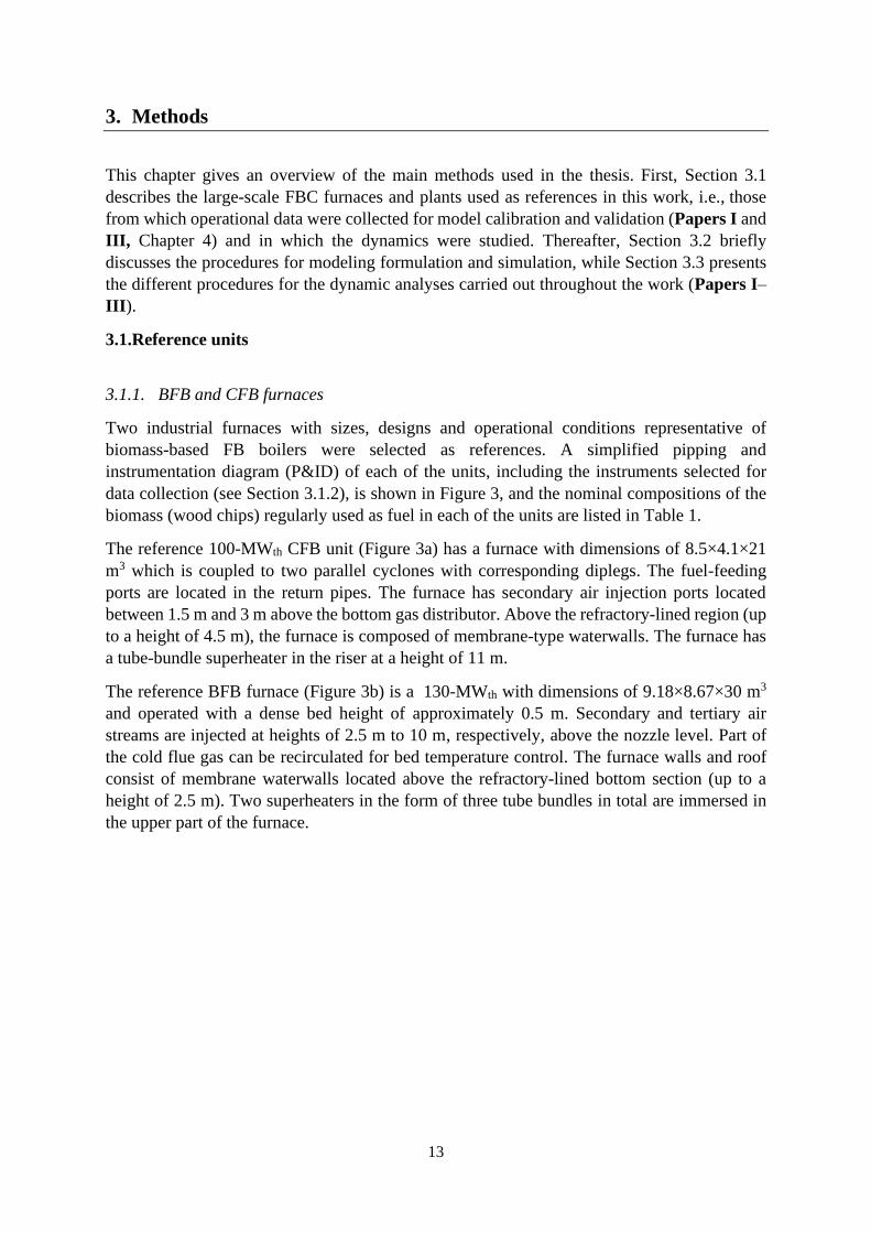
The reference 100-MWth CFB unit (Figure 3a) has a furnace with dimensions of 8.5×4.1×21

m3 which is coupled to two parallel cyclones with corresponding diplegs. The fuel-feeding

ports are located in the return pipes. The furnace has secondary air injection ports located

between 1.5 m and 3 m above the bottom gas distributor. Above the refractory-lined region (up

to a height of 4.5 m), the furnace is composed of membrane-type waterwalls. The furnace has

a tube-bundle superheater in the riser at a height of 11 m.

The reference BFB furnace (Figure 3b) is a 130-MWth with dimensions of 9.18×8.67×30 m3

and operated with a dense bed height of approximately 0.5 m. Secondary and tertiary air

streams are injected at heights of 2.5 m to 10 m, respectively, above the nozzle level. Part of

the cold flue gas can be recirculated for bed temperature control. The furnace walls and roof

consist of membrane waterwalls located above the refractory-lined bottom section (up to a

height of 2.5 m). Two superheaters in the form of three tube bundles in total are immersed in

the upper part of the furnace.

14

a) CFB unit b) BFB unit

Figure 3. Schematic piping and instrumentation diagram of the reference units. Source: Paper I

Table 1. Proximate and ultimate analyses and heating values of the reference biomass used in the reference

plants. Source: Paper I

Proximate Analysis wt% CFB furnace BFB furnace

Moisture 54.00 40.00

Volatiles 32.00 47.00

Char 13.60 12.60

Ash 0.40 0.40

Ultimate Analysis wt%

(dry ash-free)

C 50.60

5.90

43.20

0.08

0.04

H

O

N

S

HHV (dry, ash-free), MJ/kg 17.0–18.5 17.9

3.1.2 CFB-CHP plant

The reference CFB unit generates superheated steam for the production of DH and electricity.

The boiler is one of the three units that compose the DH system of the City of Karlstad in

Sweden [72], and it is operated as a mid-merit type, i.e. adjusting its output for daily changes

in heat demand. The plant is a subcritical, single-pressure steam cycle, which is typical of CHP

plants in Sweden. A simplified process diagram of the plant is shown in Figure 4, indicating

the main regulatory and supervisory control loops, as well as the names of the different process

equipment. The feedwater line flowing into the drum is first preheated in the economizer. From

the drum, the saturated water-steam mixture naturally circulates through the evaporator tubes

15

located in the furnace waterwalls. The generated steam is then superheated before expanding

in the steam turbine. DH water is produced in the last turbine condenser, whereas two additional

steam extractions are used for feedwater preheating. Note that according to this process

arrangement, the production of heat and power are linked through a constant power-to-heat

ratio (of around 0.36 in this specific case).

Figure 4. Schematic diagram of the CFB-CHP reference plant. Name tags of the main process equipment: SH:

superheater. DSH: desuperheater. ECO: economizer, HPT: high pressure turbine. IPT: intermedium pressure

turbine. LPT: low pressure turbine. OFWH: open feedwater heater. FWH: feedwater heater. DHC: district

heating condenser. CP: centrifugal pump. Supervisory and control structures are shown: L: level. F: flow, T:

temperature. Source: Paper III

3.1.2. Data acquisition

The reference units presented above were used to collect both operational plant data and design

information of the main process components. Following a systematic approach for the data

collection and analysis is required when dealing with complex plants as the ones of this work.

Thus, the following steps summarize the data acquisition process followed for collecting and

processing the datasets used in this work:

- Step 1 - Instrument and data selection: Studying the P&IDs containing the flows,

vessels, controllers, and instruments present in each of the units conforming the plants

is a mandatory first step in the data acquisition process. Subsequently, the instruments

of interest, i.e. the measurements and set points containing variables of interest for the

model development are selected and requested. Variables of interest include

temperatures, pressures, flows, levels and concentrations. In parallel to the instrument

selection, geometric design data of the modeled equipment were selected, such as

dimensions, pitch and number of tubes, existence of fins or metal thicknesses.

16

- Step 2 - Time period selection: For the steady-state calibration and validation of the

model, different operational periods at which the plants were running at diverse load

levels were requested. Steady-state datasets involved periods of 1-2 hours of operation.

Regarding transient operation, periods in which the load was increased and decreased

were requested. The transient datasets used in this work are periods of 3h of operation.

The resolution of both steady-state and transient datasets was the minimum that the

plant instruments could provide, i.e. 60 seconds.

- Step 3 - Post-processing data: Steady-state data used in this work was calculated as the

average of 30-minute measurements (see Paper I for details). For the transient

validation (see Section 4.3.3), the measured transient datasets were linearly interpolated

from the sampling time scale of 1 min into a time scale of 1 second.

3.2. Modeling and simulation

Dynamic models of thermal power plants are those capable of describing both the steady-state

behavior at several load levels (i.e. design and off-design behaviors) as well as the transient

behavior of the process when the operating conditions are changed, capturing the timescales

and physical phenomena of the changes of interest. In this work, dynamic models of the gas

and water-steam side of FBC plants are developed using Modelica [73]. The model also

includes regulation components such as controllers, ramps, steps and other mathematical

blocks. The formulated dynamic models result in a differential-algebraic system of equations

(DAE) solved by means of the numerical solver Radau IIA [74]. In order to capture the fast-

transient events typical of combustion processes, the selected time resolution for the dynamic

analysis was 1 second. This was increased to 100 seconds for steady-state analyses.

Initialization of the model was done by assigning design values to the main state variables.

To simulate the reference units, the models are first parametrized with design plant data and

after that calibrated and validated with steady-state and transient operational plant data from

the reference units described in Section 3.1. The calibration and validation of the gas-side

model with data from the BFB and CFB furnaces are described in Paper I, while the validation

and calibration of the CFB-CHP model accounting for both the gas and water-steam sides are

presented in Paper III. Figure 5 summarizes the operational datasets used for calibration

(green boxes) and validation (grey boxes), respectively. As indicated, for the reference CFB

unit the model (encompassing the gas and water-steam sides) is calibrated to match the steady-

17

state operational dataset at 100% load. For the BFB reference furnace, the model is calibrated

with steady-state data at 100% and 40% load.

Figure 5. Operational datasets acquired from the reference plants and used for model calibration (green boxes)

and validation (grey boxes). Yellow boxes refer to the gas side model and blue boxes to the integrated plant

model.

3.3. Dynamic analyses

This section describes the methods employed in the dynamic analyses for the evaluation of the

inherent and controlled transient performances of FBC plants through dynamic simulations.

3.3.1. Inherent dynamics

The inherent dynamics of a certain system are commonly evaluated through open-loop tests.

These tests involve the introduction of individual step-changes in the key process inputs when

the system is uncontrolled, after which the trajectories of the variables of interest are tracked.

Thus, an open-loop analysis enables an assessment of how the system responds to the effect of

a specific change while minimizing/cancelling the impact of the control layer. Performing this

type of tests in industrial plants is often not possible due to safety and operational constraints

as well as due to the presence of non-optimal control loops, what makes mechanistic dynamic

models a great alternative for the investigation of the process inherent dynamics.

Table 2 lists the changes studied through open-loop tests in each of the appended papers,

specifying the step magnitudes and the loads at which the boilers were running when the steps

were introduced. Process variables typically important for operation are used to characterize

the transient performances of the gas and water-steam sides, included in Table 3. The responses

of these variables are assessed in terms of the total stabilization time [ts, see Eq. (1)], which is

defined as the time it takes for a certain process variable y to remain within an error band of

±10% of the total change in steady-state values. The relative change (RC) of the process

18

variables between their initial and final steady-state values is also computed according to Eq.

(2). Figure 6 includes a simplified representation of how ts and RC are computed.

Table 2. Step changes (magnitude and variable) input in the model for the open-loop tests.

Input variable changed Simulated steps

Paper I Combustion load, Qcomb

Fuel moisture content, %H2O

-15%, ±25% and -50% at 100% load

±5% at 100% load and at 75% load

Paper II Combustion load, Qcomb

Fuel moisture content, %H2O

-15% at 100% load

+5% at 100% load

Paper III Combustion load, Qcomb ±20% at 70% load and at 80% load

Fuel heating value, HVf ±20% at 70% load and at 80% load

DH water flow, FDH ±20% at 70% load and at 80% load

DH water inlet temperature, TDH,in ±20% at 70% load and at 80% load

Table 3. Process variables tracked to characterize the inherent dynamics

Gas side

Temperature of the dense bed, Tdb [˚C]

Temperature at the top of the furnace, Ttop [˚C]

Total heat transferred to the waterwalls, Qwalls [MW]

Water-steam side

Power produced, Pel, [MW]

DH load, QDH, [MW]

DH water outlet temperature, TDH,out [˚C]

Live steam mass flow, Fsteam [kg/s]

Live steam pressure, Psteam [bar]

𝑡𝑠 = 𝜏⌋𝑦0 → 𝑦∞∓0.1(𝑦0−𝑦∞) (1)

𝑅𝐶 = 100 ∙𝑦∞−𝑦0

𝑦0 (2)

Figure 6. Schematic of how stabilization time and relative change are computed from the transient trajectory of

a certain process variable

Paper II carries out a comprehensive comparison of the transient performances of the gas sides

of BFB and CFB furnaces of the same size. For this, the stabilization times of the different

19

variables listed in Table 3 are studied through open-loop tests as a function of the characteristic

times of the main gas-side mechanisms (i.e., fluid dynamics, heat transfer and fuel conversion;

see Chapter 4).

3.3.2. Controlled dynamics

The supervisory control layer of a process plant is responsible for regulating the variables of

importance from the production point of view, i.e., driving the plant economics in a longer

timeframe [38]. In thermal power plants, the supervisory control structure works on a minute-

hour timescale, handling variations in the fuel composition and load. In particular in steam-

generating plants, such as those investigated in this work, the supervisory control system

modulates the steam flow, temperature, and pressure, so as to target production values.

Complementary to this, the regulatory control layer takes care of stabilizing the process so that

it does not drift away from acceptable operating conditions during disturbances. This translates

into the control of vessel pressures, levels, and in some cases, temperatures.

Supervisory control strategies for boilers differ in with respect to whether the power plant

output (i.e., generated power and heat) is controlled by the combustion load (i.e., air and fuel

flows into the furnace) or by the live steam control valve. The operational implications of each

of the most-common standard boiler control strategies used to provide fast load changes in

FBC plants are briefly described below, schematically shown in Figure 7 and reviewed in

Paper III.

- Boiler-following operation (BF): The master load controller manipulates the live steam

control valve, which yields a change in the live steam pressure that is corrected by the

pressure controller that manipulates the combustion load.

- Turbine-following operation (TF): The master controller uses the combustion load to

control the load, while the live steam pressure is controlled by the opening of the steam

control valve.

- Floating pressure operation (FP): In this operational strategy, the live steam pressure is

not controlled, and instead fluctuates with boiler load as a result of the energy balance

in the boiler. Thus, the load is controlled with the combustion load and the live steam

control valve remains open.

- Sliding pressure: As a variant of FP operation, the pressure is controlled but not fixed.

The set-point of the live steam pressure is a function of the boiler load (and is commonly

measured using the live steam mass flow) and it is controlled by the combustion load.

Thus, the plant load is controlled by the steam control valve opening.

- Hybrid control operation: As an enhanced version of the sliding pressure method, this

strategy combines constant pressure operation at high boiler loads with variable

pressure at lower loads (see [75] and [76]).

20

a) Fixed pressure strategies

b) Variable pressure strategies

Figure 7. Supervisory control strategies for load changes. Source: Paper III

Variable ramping rate analysis

In order to assess the performances of FBC plants at rates that are typical for industrial

operation, load changes at different ramping rates are investigated. While Paper I evaluates

the implications of load ramping speed on the in-furnace dynamics, Paper III evaluates the

load changing performance of the CFB-CHP plant when operated under different control

strategies and for several ramping rates (see Table 4). The rise time of the generated power,

i.e., the time that it takes for the output power to go through the 10%–90% response window

[77], is used in Paper III to assess the performance of each control strategy.

21

Table 4. Magnitude and rate of the load changes simulated in the variable ramping rate (VRR) analysis

Load change Ramping rate

Paper I 100%→75% -0.41%/s

-0.041%/s

Paper III

100%→50%

-0.005%/s

-0.05%/s

-0.5%/s

-5%/s

50%→40%

-0.001%/s

-0.01%/s

-0.1%/s

-1%/s

22

23

4. Dynamic model

A dynamic model of large-scale FBC plants is developed in this work, and it is used for

generating the dynamic responses, which are analyzed as described in Chapter 3 (see Papers

I–III). This chapter describes the formulation, calibration and validation of the overall dynamic

model, resulting from integrating two dynamic models: one describing the gas side of FBC

plants (described in detail in Paper I), and one describing the water-steam side (presented in

Paper III). External inputs required for the integrated model are:

- Boiler and equipment geometry, including location of fuel and air feeding injections.

- Bulk solids properties: namely the density and size of the in-furnace bulk solids.

- Riser pressure drop, i.e.

- Fuel and gas composition and properties, including feeding temperatures.

- DH inlet conditions: flow, temperature and pressure of the return DH entering the plant.

- Operational conditions dictating the operation of the reference plant, i.e. set points for

load level, live steam temperature and/or pressure, etc.

Figure 8 shows a schematic of the input/output flow diagram of the two integrated models,

including the master control governing the plant operation and the internal model variables

through which both sides are connected. The following aspects of the model integration in the

present work are particularly noteworthy:

- The flue gas stream leaving the gas side enters the water-steam side model via the

convection path.

- The furnace waterwalls transfer heat from the gas side for evaporating the biphasic

water-steam flow, which in combination with the thermal inertia of the wall material

determines the dynamics of the wall temperature. This heat transfer through the walls

and wall temperatures are represented in Figure 8 by a single arrow for simplification.

However, these are handled in the model as control volumes in each of which a dynamic

energy balance is solved (see Section 4.1 for details).

- The superheaters that are immersed in the furnace at height h extract heat from the

corresponding control volumes of the gas side while simultaneously superheating steam

in the water-steam side.

24

Figure 8. Input/output scheme of the integrated dynamic model including the master control. Source: Paper III

4.1. Gas side

The gas side (see glossary and Figure 9 for the definition and boundaries, respectively) is

described by a number of perfectly mixed control volumes (CSTR) that exchange mass and

energy (Figure 10). The domain is divided into the different fluid-dynamic regions that are

generally identified from experimental studies in large-scale FBCs [78], [79], [80]: the dense

bed and freeboard, and for CFB boilers, also the exit zone, cyclone and loop seal. The regions

that are known to exhibit a plug-flow behavior, and thus deviate from the assumption of perfect

mixing (such as the gas in the dense bed or gas and solids in the freeboard), are described in

terms of a consecution of CSTRs. The model accounts for three phases consisting of the: gas

(comprising an ideal gas mixture of nine phase components); fuel (modeled as three phase

components – fresh, dry devolatilized, and char – to account for the changes in size and density

that occur during conversion); and bulk solids (represented by a mean size). The model solves

the intercoupled dynamic energy and mass balances for each of the control volumes, computing

the temperatures and heat flows, as well as the concentrations and mass flows of each of the

phase components. These energy and mass balances are governed by three main mechanisms

defined below and briefly described in the following subsections:

- Fluid dynamics: description of the gas and solids flows within the furnace.

- Fuel conversion: drying, devolatilization and homogeneous and heterogeneous

combustion of the fuel.

- Heat transfer: Transport of thermal energy within the furnace and from/to the

waterwalls.

25

Figure 9. Schematic of the general layout and boundaries of gas side, water-steam side and membrane wall.

Green arrow is fuel, blue arrows are gas, black arrows are water-steam flows and red arrows are heat flows

Figure 10. Schematic of the dynamic model of the gas side including domain discretization and scheme of

phase and phase components. Dotted lines/arrows are exclusively present in CFB conditions. Source: Paper I

4.1.1 Fluid dynamics

In the model, the height of the dense bed is considered to be constant and is selected according

to the total riser pressure drop (handled as an input). Note that when the model is run in BFB

mode, all of the solid phase is assumed to remain in the bottom bed, i.e., solids entrainment is

neglected. When run in the CFB mode, the in-furnace fluid dynamics is a 1.5D description that

assumes, based on previous findings [81], that there is no gas flow in the wall-layers. The solids

flow is modeled in accordance with previous publications [82], [83], with the solids

entrainment from the bottom and the backflow effect at the furnace top being modeled using

expressions derived from the data in a previous study [84] [Eqs. (3) and (4), respectively]. The

26

entrained solids are assumed to flow upwards at their slip velocity, calculated from the single-

particle terminal velocity [85], which is also assumed to be the velocity at which the solids

flow downwards in the wall-layers [86]. The backmixing of solids to the waterwalls in the

freeboard is modeled according to Eq. (5) (solids clusters in the splash zone [80]), and Eqs. (6)

and (7) (transfer of the entrained to the walls in the freeboard [82], [84], [87]), respectively.

Paper I includes a detailed description of how Eqs. (3) – (7) are used in the mass balances of

the CFB gas side model.

𝑐𝑠,𝑒𝑛𝑡𝑟∙(𝑢−𝑢𝑡)

𝜌𝑔∙𝑢= 3109 ∙ (1 −

𝑢𝑡

𝑢)6.8 (3)

𝑘𝑏 = 0.85 ∙ [1

1+exp (−66∙𝑆𝑡)]

255 (4)

𝑎 = 4𝑢𝑡

𝑢 (5)

𝐾 =4𝑘

𝐷𝑒(𝑢−𝑢𝑡) (6)

𝑘 = 0.1084 ∙ (𝑢 − 𝑢𝑡) (7)

4.1.2. Fuel conversion

The model accounts for the main steps involved in the conversion of solid fuel particles typical

for FB conditions, i.e., drying and devolatilization, and char combustion, using a characteristic

time for each. The drying and devolatilization processes are driven by heat transfer and occur

simultaneously given the large fuel particle sizes in FBC units, with a combined drying and

devolatilization time as a function of the fuel particle size taken from [88]. The time for char

combustion is calculated according to the expressions for shrinking sphere conversion regime

under transport-controlled conditions. Lastly, the model includes three homogeneous reactions:

the combustion of CO, H2 and light hydrocarbons, with rates calculated according to [89] and

[90].

4.1.3. Heat transfer

The formulation of the heat transfer differs between the CFB and BFB modes. Under CFB

conditions, bed-to-wall heat transfer in a certain cell i is modeled as the combined contributions

of convection and radiation, as expressed in Eq. (8). The convective heat transfer coefficient is

modeled as a function of the solids concentration in the wall-layers according to [91]. For the

radiative contribution, the model introduces the radiation efficiency factor suggested

previously [91], according to which the radiation of heat from the core solids to the waterwalls

increases as the solids concentration in the freeboard decreases.

𝑄𝑒𝑥𝑡𝑟𝑎𝑐𝑡𝑒𝑑,𝑖 = ℎ𝑐 ∙ 𝐴𝑤 ∙ (𝑇𝑤𝑙 − 𝑇𝑤) + 𝜂𝑟𝑎𝑑 ∙ 𝜀𝑠𝑢𝑠𝑝,𝑖 ∙ 𝐴𝑤 ∙ 𝜎 ∙ (𝑇𝑐4 − 𝑇𝑤

4) (8)

When run under BFB conditions, the convective heat transfer to the waterwalls is neglected

and only radiation is accounted for. This radiative heat transfer shows a relatively low optical

thickness in the freeboard of BFB units, which allows the different surfaces to radiate heat to

27

each other. Thus, the model accounts for radiation between surfaces and volumetric cells, with

geometric view factors calculated according to [92] (for details, see Paper I). Note that even

at the low gas velocities characteristic of BFB operation, the freeboard contains a small amount

of fine solids, which are known to influence the emissivity of the volumetric cells. This cell

emissivity is computed according to Beer´s law [Eq. 9], where kvol is a tuning factor (see Section

4.3 and Paper I) that depends on the gas velocity, in order to account for the contribution of

the solids fines at different loads.

𝜀𝑣𝑜𝑙 = 1 − 𝑒−𝑘𝑣𝑜𝑙𝐿𝑝 (9)

4.2. Water-steam side

The dynamic process model of the water-steam side is built using the Modelon

ThermalPowerLibrary [93]. The different components have been modeled using the lumped

parameter approach, which is known to be a valid assumption when describing power plants at

the process level [94]. Regarding those components for which such a 0D representation is not

appropriate, e.g., a tube, a 1D discretization is applied. For all the components, geometric data

were fed into the model according to the design of the reference plant (Section 3.1.2).

In the convection path, the heat transfers on the gas and water-steam sides of the superheaters

and economizers are modeled according to Nusselt number correlations from [95], while the

evaporator tubes model uses a correlation based on the Dittus-Boelter equation. The wall

separating the two sides is modeled as a 1D domain, assuming heat accumulation with a

thermal resistance function of the wall thickness, area and conductivity.

The steam drum is modeled according to [96], solving the dynamic energy and mass balances

for the liquid and vapor volumes. Heat transfer through the drum walls and heat accumulation

in the walls are neglected. The natural circulation of the two-phase flow through the evaporator

tubes is modeled with an ideal height difference that yields a certain pressure head.

The steam turbine is described by a quasi-static model, an assumption that is found valid when

comparing its characteristic time with those of other plant components such as condensers [97].

The power generation is calculated based on the inlet and outlet steam enthalpies with a

constant dry isentropic efficiency [98]. The off-design performance is modeled according to

Stodola´s law of cones, according to which the flow area coefficient Kt is calculated as:

𝐾𝑡 =𝐹𝑛

√𝑝𝑖,𝑛𝜌𝑖,𝑛(1−(𝑝0,𝑛𝑝𝑖,𝑛

)2

)

(10)

Lastly, the steam condensers are modeled as horizontal cylindrical vessels with a hotwell at the

bottom where the condensate is accumulated. The model assumes thermodynamic equilibrium

between the two phases. A wall model separates the condensing steam from the cooling fluid,

with a heat transfer correlation for condensing steam over horizontal tubes and one based on

the logarithmic average of the inlet and outlet temperatures for the cooling media, as derived

from [95]. The deaerator is modeled in a similar manner, albeit without cooling tubes and

neglecting the heat transfer through the walls.

28

The supervisory controllers are modeled as PI controllers that are tuned according to the PID

tuning rules described by Skogestad [99]. Note that for tuning the supervisory control

structures, the regulatory control layer needs to be already tuned and kept in a closed loop. For

cascade control loops, the slave controller (i.e., the internal, faster controller) is tuned first.

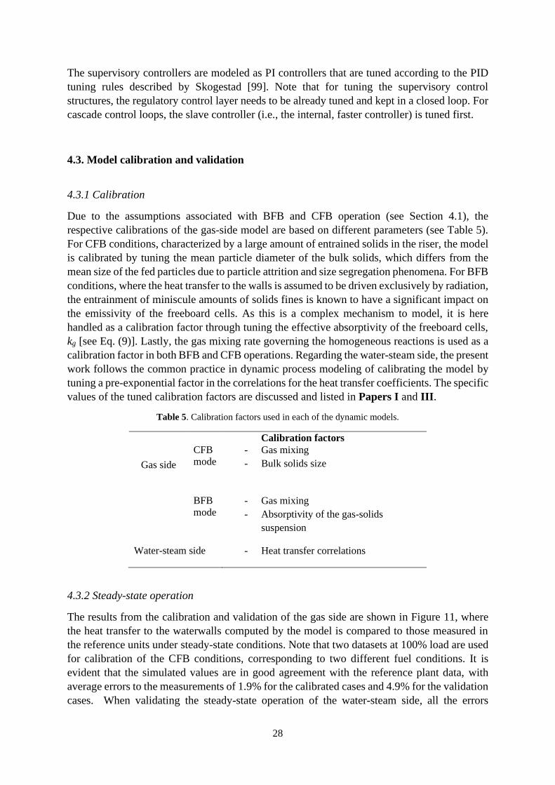
4.3. Model calibration and validation

4.3.1 Calibration

Due to the assumptions associated with BFB and CFB operation (see Section 4.1), the

respective calibrations of the gas-side model are based on different parameters (see Table 5).

For CFB conditions, characterized by a large amount of entrained solids in the riser, the model

is calibrated by tuning the mean particle diameter of the bulk solids, which differs from the

mean size of the fed particles due to particle attrition and size segregation phenomena. For BFB

conditions, where the heat transfer to the walls is assumed to be driven exclusively by radiation,

the entrainment of miniscule amounts of solids fines is known to have a significant impact on

the emissivity of the freeboard cells. As this is a complex mechanism to model, it is here

handled as a calibration factor through tuning the effective absorptivity of the freeboard cells,

kg [see Eq. (9)]. Lastly, the gas mixing rate governing the homogeneous reactions is used as a

calibration factor in both BFB and CFB operations. Regarding the water-steam side, the present

work follows the common practice in dynamic process modeling of calibrating the model by

tuning a pre-exponential factor in the correlations for the heat transfer coefficients. The specific

values of the tuned calibration factors are discussed and listed in Papers I and III.

Table 5. Calibration factors used in each of the dynamic models.

Calibration factors

Gas side

CFB

mode - Gas mixing

- Bulk solids size

BFB

mode - Gas mixing

- Absorptivity of the gas-solids

suspension

Water-steam side - Heat transfer correlations

4.3.2 Steady-state operation

The results from the calibration and validation of the gas side are shown in Figure 11, where

the heat transfer to the waterwalls computed by the model is compared to those measured in

the reference units under steady-state conditions. Note that two datasets at 100% load are used

for calibration of the CFB conditions, corresponding to two different fuel conditions. It is

evident that the simulated values are in good agreement with the reference plant data, with

average errors to the measurements of 1.9% for the calibrated cases and 4.9% for the validation

cases. When validating the steady-state operation of the water-steam side, all the errors

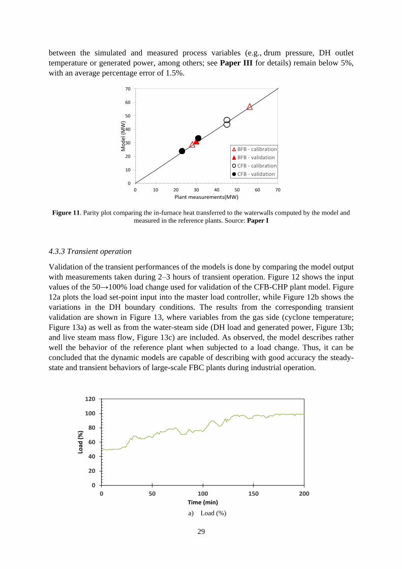
29

between the simulated and measured process variables (e.g., drum pressure, DH outlet

temperature or generated power, among others; see Paper III for details) remain below 5%,

with an average percentage error of 1.5%.

Figure 11. Parity plot comparing the in-furnace heat transferred to the waterwalls computed by the model and

measured in the reference plants. Source: Paper I

4.3.3 Transient operation

Validation of the transient performances of the models is done by comparing the model output

with measurements taken during 2–3 hours of transient operation. Figure 12 shows the input

values of the 50→100% load change used for validation of the CFB-CHP plant model. Figure

12a plots the load set-point input into the master load controller, while Figure 12b shows the

variations in the DH boundary conditions. The results from the corresponding transient

validation are shown in Figure 13, where variables from the gas side (cyclone temperature;

Figure 13a) as well as from the water-steam side (DH load and generated power, Figure 13b;

and live steam mass flow, Figure 13c) are included. As observed, the model describes rather

well the behavior of the reference plant when subjected to a load change. Thus, it can be

concluded that the dynamic models are capable of describing with good accuracy the steady-

state and transient behaviors of large-scale FBC plants during industrial operation.

a) Load (%)

0

10

20

30

40

50

60

70

0 10 20 30 40 50 60 70

Mo

del

(M

W)

Plant measurements(MW)

BFB - calibration

BFB - validation

CFB - calibration

CFB - validation

0

20

40

60

80

100

120

0 50 100 150 200

Load

(%

)

Time (min)

30

b) DH inlet temperature and mass flow

Figure 12. Input trajectories to the integrated plant model for transient operation validation. Source: Paper III

a) Tcyclone

b) QDH and Pel

450

470

490

510

530

550

570

60

62

64

66

68

70

72

74

76

0 50 100 150 200

Mas

s fl

ow

(kg

/s)

Tem

per

atu

re (

˚C)

Time (min)

DH T_inDH mass flow

31

c) 𝐹𝑠𝑡𝑒𝑎𝑚

Figure 13. Transient validation of the main process variables of the gas and water-steam sides. The plots

compared the simulated and measured trajectories over a 3h load increase for a) cyclone temperature b) DH heat

production and generated power and c) mass flow of live steam. Sources: Paper I and III

32

33

5. Selected results and discussion

The most important findings from the three appended papers are presented and discussed in

this chapter, the structure of which is aligned with the research questions formulated in Chapter

1. First, the inherent dynamic behaviors of FBC plants are presented, both for the gas side

(Papers I and II) and at the plant (gas and water-steam sides) level (Paper III). Second, the

performances of FBC plants under different supervisory control strategies are addressed.

Lastly, the dynamic interplay between the gas and water-steam sides in FBC plants is

discussed.

5.1.Inherent dynamics of FBC plants

5.1.1 Gas side

The inherent dynamics of the gas sides of the CFB and BFB reference furnaces are analyzed

and compared in Figure 14. Figure 14, a and b shows the open-loop transient responses of the

main process variables of the gas side when the load is reduced in a single step from 100% to

75% in the CFB and BFB, respectively. In the CFB furnace, the bottom temperature is reduced

to a lesser extent than the temperature at the top of the furnace because: (i) the dense bed has

much larger solids flows than the top of the reactor; and (ii) at lower loads, i.e., at lower gas

velocities, the relative content of fuel in the bottom region increases, whereas it decreases in

the upper region. Besides, due to the larger heat capacity of the bottom region (consequence of

the solids inventory), the temperature response in the bottom region is slower than that at the

furnace top. In the BFB furnace (Figure 14b), the differences in heat capacity between the

bottom and top regions are more pronounced, which explains the larger differences observed

in these regions for the transient responses and the stabilization times of the temperatures.

Figure 14, c–f shows the computed stabilization times (ts) and relative changes (RC) of the

CFB and BFB reference furnaces when the magnitude of the introduced load change is varied.

In line with the observations mentioned above, it is evident that the stabilization time of the

dense bed is always longer than that at the top of the furnace for all the cases investigated,

although the relative change is smaller. Thus, these differences are maximized in the BFB

furnace, with the stabilization time in the dense bed being around 20 minutes, compared to 30–

100 seconds at the top of the furnace. Another important aspect highlighted in Figure 14, c and

e is that when the load is incremented, the stabilization times are significantly shorter than

those related to a load reduction of the same magnitude. This aspect, which has been previously

reported for other thermal processes (see [43] and [100]) and is explained in detail in Papers I

and II, reflects the fact that a load reduction relies on the heat transfer to the waterwalls, a

process that is generally slower than the heat release due to fuel conversion driving the

temperature change under a load increase. As shown in Figure 14, the dynamics of the heat

transfer to the waterwalls Qwall are largely driven by the in-furnace temperatures, thus

stabilization is achieved just before/after the temperature at the furnace top stabilizes.

34

a) Open-loop responses of the in-furnace

CFB process variables for a -25% step

change

b) Open-loop responses of the in-furnace

BFB process variables for a -25% step

change

c) Stabilization times of the in-furnace

CFB variables for various load step

changes

d) Relative changes of the in-furnace CFB

variables for various load step changes

e) Stabilization times of the in-furnace

BFB variables for various load step

changes

f) Relative changes of the in-furnace BFB

variables for various load step changes

Figure 14. Inherent dynamics of the gas sides of the reference CFB and BFB furnaces, expressed as variable

trajectories, stabilization times (ts) and relative changes (RC). Source: Paper I.

To analyze the dependencies of the stabilization times of the gas side on the three main

mechanisms taking place in the furnace (fluid dynamics, fuel conversion and heat transfer),

additional open-loop tests are performed for the -25% load reduction, whereby the

characteristic times of each of the mechanisms (defined and varied as shown in Table 6) are

varied independently (for details, see Paper II). A representative selection of the runs is plotted

in Figure 15a (reference BFB furnace, note the double y-axis) and Figure 15b (CFB furnace

upscaled to the same thermal capacity as the BFB reference furnace). Table 6 formulates

simplified mathematical expressions that relate the stabilization times of the three gas-side

0

500

1000

1500

2000

2500

25% -10% -25% -50%

ts (

s)

Load change (%)

Ttop

Tdb

Qwall

0

5

10

15

20

25

30

35

40

45

50

-10% -25% -50%

RC

(%

)

Load change (%)

Ttop

Tdb

Qwall

0

500

1000

1500

2000

2500

25% -10% -25% -50%

ts (

s)

Load change (%)

Ttop Tdb

Qwall

0

5

10

15

20

25

30

35

40

45

50

-10% -25% -50%

RC

(%

)

Load change (%)

Ttop

Tdb

Qwall

30

32

34

36

38

40

42

44

46

48

50

725

745

765

785

805

825

845

865

885

-200 300 800 1300

He

at

(MW

)

Tem

pe

ratu

re (

˚C)

Time (s)

TtopTdbQwall

30

35

40

45

50

55

60

770

820

870

920

970

1020

1070

1120

-200 800 1800 2800

He

at

(MW

)

Tem

pe

ratu

re (

˚C)

Time (s)

TtopTdbQwall

35

variables monitored (heat extracted from the furnace and temperatures at the furnace bottom

and top of the furnace) to the characteristic times of the above-mentioned furnace mechanisms.

Table 6. Characteristic times of the main in-furnace mechanisms of CFB and BFB furnaces. The table shows

how these have been varied in the model to evaluate their impacts on the in-furnace dynamics. Note that the

fluid dynamics characteristic time of the BFB furnace has not been varied. Source: Paper II.

Mechanism Characteristic time Variable varied

CFB BFB CFB BFB

Fluid dynamics 𝜏𝐹𝐷,𝐶𝐹𝐵 = 𝜏𝑟𝑖𝑠𝑒𝑟 +

𝜏𝑐𝑦𝑐𝑙𝑜𝑛𝑒 + 𝜏𝑙𝑜𝑜𝑝−𝑠𝑒𝑎𝑙

𝜏𝐹𝐷,𝐵𝐹𝐵 = 𝜏𝑔𝑎𝑠 Size of loop seal

(for CFB) -

Fuel conversion 𝜏𝐹𝐶 = 𝑡𝑐ℎ𝑎𝑟 Char conversion time

Heat transfer 𝜏𝐻𝑇 =

∑ 𝑀𝑖𝐶𝑝,𝑖

∑ 𝐹𝑖𝐶𝑝,𝑖

Solids heat capacity

In agreement with the discussion coupled to Figure 14, the dense bottom bed of the BFB

furnace takes much longer to stabilize (600–1500 seconds) than the temperature at the furnace

top and the heat extracted through the walls. It can be seen that the stabilization times at the

furnace bottom correspond roughly to the sum of the characteristic times of the two

mechanisms present in the dense bottom bed, i.e., the fuel conversion and the heat transfer [see

Eq. (11)]. In contrast, the temperature at the furnace top and the heat transfer to the walls

stabilize in 60–80 seconds and 40–70 seconds, respectively, as a consequence of Qwall being

driven by the change in effective gas emissivity forced by the varied presence of solids fines

entrained by the gas. Given the very low thermal inertia of the upper regions of the BFB

furnace, its temperature dynamic behavior can be expressed as a function of the residence time

of the gas triggering the change in gas emissivity, and to a minor extent [see Eq. (12)], the

stabilization time of the temperature exiting the bottom region. Since Qwall depends mainly on

the gas temperature and effective emissivity, its stabilization time can be approached as that of

the temperature at the furnace top [Eq. (13)].

a) BFB furnace

36

b) CFB furnace

Figure 15. Stabilization times of the gas sides of the BFB and CFB furnaces under variations of the

characteristic times of the three in-furnace mechanisms (FC, fuel conversion; FD, fluid dynamics; HT, heat

transfer). Note that the characteristic time of FD is not varied in the BFB furnace. Source: Paper II.

When analyzing the stabilization times of the monitored variables in the CFB furnace, a

relatively uniform effect of the three mechanisms considered for the CFB conditions is

observed on the gas-side temperatures. Furthermore, in the bottom region, the stabilization time

can be directly approximated as the sum of the three characteristic times [Eq. (14)]. Thus, even

though the changes in fluid dynamics, fuel conversion and heat transfer are occurring in

parallel, the tails of each of these mechanisms follow each other and add up sequentially to

give the total stabilization time. As for the temperature in the upper furnace, its stabilization

generally occurs some 30% faster than that at the furnace bottom [Eq. (15)]. Lastly, the

dynamics of the heat transfer to the waterwalls are found to be sensitive to all the investigated

variations, although they are predominantly influenced by the fuel conversion time [Eq. (16)].

These results may be of importance when assessing the transient capabilities of the gas side of

a given FB furnace with a certain size, fuel and bulk solids. The expressions in Table 7

represent a simple way to estimate the impacts of specific changes in the gas velocity, fuel size

or composition, or a change in the solids inventory on the dynamic behaviors of key in-furnace

variables.

37

Table 7. Simplified expressions for the dependency of the stabilization times (ts) of the gas side on the

characteristic times of the three in-furnace mechanisms (FC, fuel conversion; FD, fluid dynamics; HT, heat

transfer). Source: Paper II.

Unit Variable Expression

BFB

Tdb 𝑡𝑠,𝐷𝐵 ≈ 𝜏𝐹𝐶 + 𝜏𝐻𝑇 (11)

Ttop 𝑡𝑠,𝑡𝑜𝑝 ≈ 𝜏𝐹𝐷 + 0.05 𝑡𝑠,𝐷𝐵 (12)

Qwall 𝑡𝑠,𝑄 ≈ 𝑡𝑠,𝑡𝑜𝑝 (13)

CFB

Tdb 𝑡𝑠,𝐷𝐵 ≈ 𝜏𝐹𝐶 + 𝜏𝐻𝑇 + 𝜏𝐹𝐷 (14)

Ttop 𝑡𝑠,𝑡𝑜𝑝 ≈ 0.7 𝑡𝑠,𝐷𝐵 (15)

Qwall 𝑡𝑠,𝑄 ≈ 𝜏𝐹𝐶 (0.2 𝜏𝐹𝐷 + 0.5 𝜏𝐻𝑇) (16)

5.1.1 CFB-CHP plant

The computed stabilization times (in minutes) of the main process variables (i.e., generated

power, DH production, live steam mass flow, DH outlet temperature, live steam pressure, and

in-furnace heat transfer to the walls) when performing open-loop tests in the CFB-CHP plant

with step variations of the operational inputs (combustion load, DH flow, DH inlet temperature

and fuel heating value) are shown in Figure 16. First, it is evident from comparing Figure 16a

(-20% steps) and Figure 16b (+20% steps) that, as occurred within the gas side, the process

tends to stabilize faster (on average, 15% shorter stabilization times) when heat is added to the

system, i.e., when the combustion load, fuel heating value and DH inlet temperatures are

increased. When comparing the stabilization times of the different variables, the live steam

pressure and mass flow are found to be the fastest to reach stabilization within the water-steam

side, averaging 5 minutes for the investigated cases, which is comparable to the gas-side

variable added in Figure 16, i.e., Qwall. The generated power stabilizes within 8 minutes on

average, whereas the outlet DH temperature and the condenser heat load are the slowest

variables to reach stabilization, with average times of 10 and 13 minutes, respectively. Figure

16 also shows that the process transient response is the fastest to react to changes in the DH

mass flow, whereas the disturbances linked to the furnace, i.e., the combustion load and fuel

heating value, yield the slowest stabilization times, averaging 11 and 13 minutes, respectively,

for the cases investigated.

38

a) -20% step

b) +20% step

Figure 16. Inherent dynamics of the CFB-CHP plant, computed as the stabilization times (ts) of the main

process variables for different process disturbances, i.e., step-changes in Qcomb, FDH, TDH,in and HVf. Source:

Paper III.

5.2. Controlled dynamics

The simulated trajectories of the power generated by the reference CFB-CHP plant when the

load is changed from 100% to 50% at different ramping rates under each of the investigated

control strategies are plotted in Figure 17. While Figure 17, a and b (i.e., the slowest ramping

rates investigated, at -0.005 and -0.05%/s, respectively) show that for all the tested control

strategies, the plant is capable of executing load changes at the same rate as the set-point is

varied. Figure 17, c and d (i.e., the fastest ramping rates investigated at -0.5 and -5.0%/s,

respectively) present noticeable differences between the control structures. It is clear that the

control strategies that manipulate the steam valve opening to regulate the plant load, i.e.,

Hybrid and BF, provide fast power output changes that are able to follow the set-point. In

contrast, the control strategies that manipulate the combustion load, i.e., FP and TF, provide

considerably slower load changes, with rising times of 6 minutes and 4 minutes, respectively,

and stabilization times of up to 10 minutes. This can be explained by the dynamic effect of the

control valve, which uses the energy accumulated in the drum and superheater tubes to generate

fast, temporary changes in the steam pressure and flow, which quickly propagate to the turbine.

Figure 18 displays the live steam pressure prior to the control valve for the fastest ramping rate

0

5

10

15

20

25

Stab

iliza

tio

n t

ime

(m

in)

Qcomb FDH TDH,in HVf

Pel QDH Fsteam TDH,out Psteam Qwall

0

5

10

15

20

25

Stab

iliza

tio

n t

ime

(min

)

QcombFDH TDH,in HVf

Pel QDH Fsteam TDH,out Psteam Qwall

39

under TF, BF and Hybrid operation. It is clear that the rapid changes in power output provided

by the Hybrid and BF strategies are achieved at the expense of steam throttling, caused by fast

valve closing. The overshoot in the pressure trajectory is up to +30% for the BF case, as

compared for instance to +0.01% for the TF case. This temporary overshoot can be directly

linked to exergy losses and, therefore, loss of available work, resulting in a period of low

process efficiency that lasts until the pressure is stabilized. Under FP operation, where the

steam valve remains fully open during all the operational window, the opposite occurs:

although the plant response is considerably slower due to the thermal inertia associated with

the gas side, the throttling losses during the process transient response are minimized.

a) Very slow (-0.005%/s) b) Slow (-0.05%/s)

c) Fast: (-0.5%/s) d) Very fast (-5%/s)

Figure 17. Responses of the generated power (in % of design power) compared to the load set-point (SP) for the

100%→50% load change under different control strategies and ramping rates. FP, Floating pressure; TF,

turbine-following; BF, boiler-following. Source: Paper III.

Figure 18. Live steam pressures compared to the set-point (SP) for the very fast (-5.0%/s) ramping rate of the

100%→50% load change. Source: Paper III.

40

60

80

100

120

-2 3 8 13 18%

of

de

sig

n p

ow

er

Time (min)

FP SPTF BFHybrid

40

60

80

100

120

-2 1 4 7 10

% o

f d

esi

gn

po

we

r

Time (min)

FP SPTF BFHybrid

40

60

80

100

120

-100 0 100 200 300

% o

f d

esig

n p

ow

er

Time (min)

FP SPTF BFHybrid

40

60

80

100

120

-2 1 4 7 10

% o

f d

esi

gn

po

we

r

Time (min)

FP SPTF BFHybrid

40

5.3.Dynamic interaction between the gas and water-steam sides

Assuming a quasi-static transient behavior for the gas side is a commonly used approach when

modeling the dynamics of combustion plants because it yields substantial savings related to the

complexity and computational cost of the model. Based on the results obtained in Papers I–

III, the dynamic interplay between the gas and water-steam sides in large-scale FBC plants can

be explored.

Table 8 summarizes the inherent stabilization times computed for the main process variables

of the gas and water-steam sides. Table 8 lists only those scenarios that relate to the -20%/-

25% load reductions driven by decreases in the fuel input flow. These have been chosen in

order to allow for the comparison, since stabilization times increase with the magnitude of the

load change (for details, see Paper I) and vary depending on the change-driving parameter.

Due to the large differences in dynamics between the bottom and top regions of the furnace in

BFB units, the stabilization times of the corresponding temperatures in such units are presented

separately. It is evident that the stabilization times are of the same order of magnitude in both

the gas sides and the water-steam sides of CFB furnaces. In contrast, in BFBs, the relevant in-

furnace parameters interfacing with the water-steam side – the heat extracted in the furnace

and the flue gas temperature before the convection pass (i.e., the top/outlet furnace

temperature) – exhibit dynamics that are one order of magnitude faster than the water-steam

side.

Table 8. Summary of the inherent stabilization times of the gas and water-steam sides of the investigated units.

Variable Inherent stabilization times (min)

Gas side CFB furnaces BFB furnaces

Temperatures 3–21 Tdb: 10–26 Ttop: 1–1.5

Heat transfer to waterwalls 2–10 0.5–1.0

Water-steam side

Live steam pressure and mass flow 10

Power generation 8

DH temperatures and heat flows 13–15

Paper I analyzes the responses of the gas side variables when the load change is introduced as

a step function and at two different rates that are typical of industrial operation (see Figure

19a). As can be seen in the response trajectories included in Figure 19b, the inherent dynamics

observed for the open-loop responses disappear as the rate of the load change is slowed,

eventually yielding a ramp-like response for the slowest rate in the temperature at the furnace

top and the heat extracted through the furnace walls. This observation indicates that those

variables adopt a pseudo-steady-state behavior, i.e., at any time during load ramping, the

variables adopt the same values that they would have under steady-state conditions. Generally,

this effect arises when the load change is introduced at a rate with a longer characteristic time

than the inherent stabilization time of the variable. Note that the temperature in the dense bed,

with an inherent stabilization time longer than 600 seconds according to Table 8, does not

follow the load ramp and it displays some dynamic behavior well beyond 10 minutes.

41

a) Input load changes b) Responses of the CFB furnace

Figure 19. Variable ramping rate (VRR) test in the gas side of the CFB furnace. Source: Paper I.

Therefore, it can be concluded that for an accurate prediction of the transient performance of

FBC plants, the description of the dynamics of the gas side is crucial, especially when

investigating changes over characteristic times that are shorter than the inherent dynamics of

the gas side, as well as when the variables of interest are those connected to the live steam. As

shown in Table 8, the response times of variables such as the generated power or the live stem

pressure are very much reliant on the stabilization times of the gas side which, based on the

investigation presented in Paper II, are indeed a function of the fuel and bulk solids properties,

among other operational conditions. While these findings are of special importance for CFB

furnaces, assuming a quasi-static behavior for the gas side might suffice to describe the

transient operation of BFB plants.

These results are relevant when assessing the transient capabilities of FBC plants to provide

load changes in short timeframes on a regular basis, as needed for instance for primary control

reserve (characterized by response times in the order of 30 seconds in most European markets).

Furthermore, fast load ramping would yield undesired temporary emissions (as indicated by

the results in Paper I), highlighting the importance of a dynamic model of the gas side for a

robust assessment of the flexibility capabilities of FBC units.

0

20

40

60

80

100

120

-200 300 800 1300

Loa

d (

%)

Time (s)

Step

-25%/60s

-25%/600s

42

43

6. Conclusions

This thesis analyzes the dynamic behaviors of commercial-scale fluidized bed combustion

plants for heat and power production. The work involves the development and use of

mechanistic dynamic models of both the gas and water-steam sides of bubbling and circulating

FBCs. Two industrial-scale plants are used to acquire steady-state and transient operational

datasets for calibration and validation of the models, as they are used as reference cases for the

performed dynamic analyses.

With respect to the analyses of the inherent dynamics of FBC plants, the following can be

concluded:

- Evaluation of the impact of the thermal inertia created by the bulk solids on the in-

furnace dynamics of FBC plants reveals that regions with large heat capacities, such as

the bottom of the furnace in BFB units, take up to 10-times longer to stabilize than does

the furnace top. CFB furnaces show a more even distribution of solids throughout the

furnace, which yields stabilization times that are more similar across the different

regions. While the stabilization times of the gas sides of CFB combustors are found to

be dependent upon the characteristic times of the main in-furnace mechanisms (i.e., fuel

conversion, heat transfer and fluid dynamics), the dynamics of BFB units are driven

mainly by the residence time of the gas. For this reason, the heat transferred to the

waterwalls displays faster transient responses in BFB units than in CFB combustors.

- Due to reduced residence time of the gas and water-steam flows, FBC plants respond

faster to changes when running at higher loads. In addition, changes which imply a heat

removal from the system (e.g. decreasing combustion or DH load or increasing the fuel

moisture) leads to slower transients than the inverse.

- Lastly, it can be concluded that although the dynamic behaviors of the gas sides of FBC

plants can be assumed to be quasi-static when operated at rates that are typical of heat-

driven operation, dynamic modeling of the gas side is critical for accurate prediction of

the process dynamics when assessing faster operation. This aspect attains greater

importance in CFB combustors because the in-furnace transients are found to be of the

same magnitude as those of the water-steam side, while the in-furnace responses of

BFB units are found to be one order of magnitude faster than those of the water-steam

side.

Regarding control and operational strategies to improve the operational flexibility of FBC

plants, the following is concluded:

- Implementing supervisory control strategies can have a strong positive impact on

maximizing the load change capabilities of FBC plants. While control strategies for

load changes based on modifying the fuel input flow can provide changes in the order

of 5%/min, strategies that manipulate the live steam control valve can follow changes

in generated electricity at rates as fast as -5%/s. The results show that the increased

ramping capabilities offered by these strategies come at the expense of lowered thermal

efficiency due to steam throttling, revealing a trade-off between flexibility and

efficiency, as well as the need for economic optimization.

44

Furthermore, other constraints must be considered when assessing the transient operation

capabilities of FBC plants, such as thermal stresses in key components, undesired pollutant

emissions, and the dynamics of subsystems outside the scope of this work (e.g., the fuel

handling system).

6.1. Further work

Based on the outcomes and findings of this thesis, new research tasks can be proposed that

would likely further our understanding of the transient operational capabilities of large-scale

FB units, some of which are listed below.

- As the demand for biofuels increases and the yearly-average capacity utilization of

conventional FB boilers remains at low levels (23%-40% in Sweden, depending on the

supply side – district heating or industry), the retrofit of FBC plants into polygeneration

facilities represents a promising alternative way for FBCs to promote their standing as

a key technology for the transition towards a sustainable energy system. It is foreseen

that in such a scenario, the dynamic interplay between heat, power and gas production

will be crucial for maximizing plant utilization, for understanding the plant capabilities

to operate in specific power markets, and for establishing its role as a variation

management tool for the electricity system. The dynamic models developed in this

thesis could be adapted to account for the retrofits and could subsequently be used to

investigate the transient operation capabilities of these facilities.

- The use of large-scale FB reactors for thermochemical energy storage (TCES) through

the cycling of solid systems, such as carbonates and redox metals, is gaining global

recognition as an efficient storage technology with possibilities in relation to energy

shipping. If deployed in a renewable energy generation facility, such as a wind farm or

a concentrated solar power (CSP) plant, the transient capabilities of the process would

play a crucial role in the effective deployment of the technology. Moreover, advanced

control structures could enhance the transient performance of the process, optimizing

the operation for the timescales required by the system. Thus, the dynamic models

developed in this work and the insights acquired on the dynamics of large-scale FB

reactors are valuable for investigating TCES processes based on solids cycling.

- Using model order reduction methods, the high-fidelity models developed in this thesis

could be reduced to simpler models that are capable of describing the transient

operation of the plants at a much lower computational cost. These simpler models, after

verification and validation, could be used to develop model predictive control (MPC)

strategies for advanced and robust process control.

45

References

[1] UNFCCC, “Paris Agreement,” Conf. Parties its twenty-first Sess., no. December, p. 32, 2015,

doi: FCCC/CP/2015/L.9/Rev.1.

[2] Artur Runge and E. C. Metzger, “A Clean Planet for all Vision for a Clean Planet by 2050,” Eur.

Comm., no. November, p. 393, 2018.

[3] European Commission, “Roadmap 2050,” Policy, no. April, pp. 1–9, 2012, doi: 10.2833/10759.

[4] International Energy Agency, “Renewables 2019,” 2019.

[5] International Renewable Energy Agency, IRENA (2019), Global Energy Transformation: A

Roadmap to 2050. 2019.

[6] IEA, “World Energy Outlook (2020),” Paris, 2020.

[7] M. de Groot, W. Crijns-Graus, and R. Harmsen, “The effects of variable renewable electricity

on energy efficiency and full load hours of fossil-fired power plants in the European Union,”

Energy, vol. 138, pp. 575–589, 2017, doi: 10.1016/j.energy.2017.07.085.

[8] M. A. Gonzalez-Salazar, T. Kirsten, and L. Prchlik, “Review of the operational flexibility and

emissions of gas- and coal-fired power plants in a future with growing renewables,” Renew.

Sustain. Energy Rev., vol. 82, no. July 2017, pp. 1497–1513, 2018, doi:

10.1016/j.rser.2017.05.278.

[9] J. Beiron, R. M. Montañés, F. Normann, and F. Johnsson, “Flexible operation of a combined

cycle cogeneration plant – A techno-economic assessment,” Appl. Energy, vol. 278, no. August,

p. 115630, 2020, doi: 10.1016/j.apenergy.2020.115630.

[10] L. Göransson, M. Lehtveer, E. Nyholm, M. Taljegard, and V. Walter, “The benefit of

collaboration in the North European electricity system transition—System and sector

perspectives,” Energies, vol. 12, no. 24, 2019, doi: 10.3390/en12244648.

[11] J. Koornneef and M. Junginger, “Development of fluidized bed combustion — An overview of

trends , performance and cost,” Prog. Energy Combust. Sci., vol. 33, pp. 19–55, 2007, doi:

10.1016/j.pecs.2006.07.001.

[12] P. Basu, Circulating fluidized bed boilers: Design, operation and maintenance. 2015.

[13] M. Gao, F. Hong, and J. Liu, “Investigation on energy storage and quick load change control of

subcritical circulating fluidized bed boiler units,” Appl. Energy, vol. 185, pp. 463–471, 2017,

doi: 10.1016/j.apenergy.2016.10.140.

[14] H. Zhang, M. Gao, F. Hong, J. Liu, and X. Wang, “Control-oriented modelling and investigation

on quick load change control of subcritical circulating fluidized bed unit,” Appl. Therm. Eng.,

vol. 163, no. September, p. 114420, 2019, doi: 10.1016/j.applthermaleng.2019.114420.

[15] K. Atsonios, A. Nesiadis, N. Detsios, K. Koutita, N. Nikolopoulos, and P. Grammelis, “Review

on dynamic process modeling of gasification based biorefineries and bio-based heat & power

plants,” Fuel Process. Technol., vol. 197, no. March 2019, p. 106188, 2020, doi:

10.1016/j.fuproc.2019.106188.

[16] F. Johnsson, H. Thunman, and D. Pallarès, “Future applications of circulating fluidized-bed

technology,” in CFB-13, 2021, pp. 26–35.

[17] Z. Guo, Q. Wang, M. Fang, Z. Luo, and K. Cen, “Thermodynamic and economic analysis of

polygeneration system integrating atmospheric pressure coal pyrolysis technology with

circulating fluidized bed power plant,” Appl. Energy, vol. 113, pp. 1301–1314, 2014, doi:

46

10.1016/j.apenergy.2013.08.086.

[18] C. Heinze, J. May, J. Peters, J. Ströhle, and B. Epple, “Techno-economic assessment of

polygeneration based on fluidized bed gasification,” Fuel, vol. 250, no. February, pp. 285–291,

2019, doi: 10.1016/j.fuel.2019.04.020.

[19] G. Zsembinszki, A. Sole, C. Barreneche, C. Prieto, A. I. Fernández, and L. F. Cabeza, “Review

of reactors with potential use in thermochemical energy storage in concentrated solar power

plants,” Energies, vol. 11, no. 9, 2018, doi: 10.3390/en11092358.

[20] S. Padula, C. Tregambi, R. Solimene, R. Chirone, M. Troiano, and P. Salatino, “A novel

fluidized bed ‘ thermochemical battery ’ for energy storage in concentrated solar thermal

technologies,” Energy Convers. Manag., vol. 236, p. 113994, 2021, doi:

10.1016/j.enconman.2021.113994.

[21] G. Martinez Castilla, D. C. Guio-Perez, S. Papadokonstantakis, D. Pallarès, and F. Johnsson,

“Techno-economic assessment of calcium looping for thermochemical energy storage with CO2

capture,” Energies, vol. accepted f, 2021.

[22] N. Kumar, S. Besuner, S. Lefton, D. Agan, and D. Hilleman, “Power plant cycling costs,”

Sunnyvale, California, 2012.

[23] L. Göransson, J. Goop, M. Odenberger, and F. Johnsson, “Impact of thermal plant cycling on

the cost-optimal composition of a regional electricity generation system,” Appl. Energy, vol.

197, pp. 230–240, 2017, doi: 10.1016/j.apenergy.2017.04.018.

[24] W. L. Luyben, Plantwide dynamic simulators in chemical processing and control. New York:

Marcel Dekker, 2002.

[25] F. Alobaid, N. Mertens, R. Starkloff, T. Lanz, C. Heinze, and B. Epple, “Progress in dynamic

simulation of thermal power plants,” Prog. Energy Combust. Sci., vol. 59, pp. 79–162, 2017,

doi: 10.1016/j.pecs.2016.11.001.

[26] A. Gómez-Barea and B. Leckner, “Modeling of biomass gasification in fluidized bed,” Prog.

Energy Combust. Sci., vol. 36, no. 4, pp. 444–509, 2010, doi: 10.1016/j.pecs.2009.12.002.

[27] I. Avagianos, D. Rakopoulos, S. Karellas, and E. Kakaras, “Review of Process Modeling of

Solid-Fuel Thermal Power Plants for Flexible and Off-Design Operation,” Energies, vol. 13, no.

6587, 2020, doi: doi:10.3390/en13246587.

[28] R. M. Montañés, “Transient performance of combined cycle power plant with absorption based

post-combustion CO2 capture: dynamic simulations and pilot plant testing,” NTNU, 2018.

[29] A. P. Under, T. H. E. Clean, and E. Ministerial, “Thermal Power Plant Flexibility.”

[30] J. Beiron, R. M. Montañés, and F. Normann, “Operational Flexibility of Combined Heat and

Power Plant With Steam Extraction Regulation,” in Proceedings of 11th International

Conference on Applied Energy, 2019, pp. 1–4.

[31] E. Mollenhauer, A. Christidis, and G. Tsatsaronis, “Increasing the Flexibility of Combined Heat

and Power Plants With Heat Pumps and Thermal Energy Storage,” vol. 140, no. February, pp.

1–8, 2018, doi: 10.1115/1.4038461.

[32] P. Li, H. Wang, Q. Lv, and W. Li, “Combined heat and power dispatch considering heat storage

of both buildings and pipelines in district heating system for wind power integration,” Energies,

vol. 10, no. 7, 2017, doi: 10.3390/en10070893.

[33] D. Romanchenko, J. Kensby, M. Odenberger, and F. Johnsson, “Thermal energy storage in

district heating: Centralised storage vs. storage in thermal inertia of buildings,” Energy Convers.

Manag., vol. 162, no. January, pp. 26–38, 2018, doi: 10.1016/j.enconman.2018.01.068.

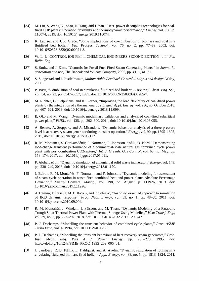
47

[34] M. Liu, S. Wang, Y. Zhao, H. Tang, and J. Yan, “Heat–power decoupling technologies for coal-

fired CHP plants: Operation flexibility and thermodynamic performance,” Energy, vol. 188, p.

116074, 2019, doi: 10.1016/j.energy.2019.116074.

[35] K. Laursen and J. R. Grace, “Some implications of co-combustion of biomass and coal in a

fluidized bed boiler,” Fuel Process. Technol., vol. 76, no. 2, pp. 77–89, 2002, doi:

10.1016/S0378-3820(02)00021-8.

[36] W. L. I, “CONTROL iOR FlitI m CHEMICAL ENGINEERS SECOND EDITION- a I,” Pet.

Refin. Eng.

[37] S. Stultz and J. Kitto, “Controls for Fossil Fuel-Fired Steam Generating Plants,” in Steam: its

generation and use, The Babcok and Wilcox Company, 2005, pp. 41–1, 41–21.

[38] S. Skogestad and I. Postlethwaite, Multivariable Feedback Control. Analysis and design. Wiley,

2006.

[39] P. Basu, “Combustion of coal in circulating fluidized-bed boilers: A review,” Chem. Eng. Sci.,

vol. 54, no. 22, pp. 5547–5557, 1999, doi: 10.1016/S0009-2509(99)00285-7.

[40] M. Richter, G. Oeljeklaus, and K. Görner, “Improving the load flexibility of coal-fired power

plants by the integration of a thermal energy storage,” Appl. Energy, vol. 236, no. October 2018,

pp. 607–621, 2019, doi: 10.1016/j.apenergy.2018.11.099.

[41] E. Oko and M. Wang, “Dynamic modelling , validation and analysis of coal-fired subcritical

power plant,” FUEL, vol. 135, pp. 292–300, 2014, doi: 10.1016/j.fuel.2014.06.055.

[42] A. Benato, A. Stoppato, and A. Mirandola, “Dynamic behaviour analysis of a three pressure

level heat recovery steam generator during transient operation,” Energy, vol. 90, pp. 1595–1605,

2015, doi: 10.1016/j.energy.2015.06.117.

[43] R. M. Montañés, S. GarÐarsdóttir, F. Normann, F. Johnsson, and L. O. Nord, “Demonstrating

load-change transient performance of a commercial-scale natural gas combined cycle power

plant with post-combustion CO2capture,” Int. J. Greenh. Gas Control, vol. 63, no. May, pp.

158–174, 2017, doi: 10.1016/j.ijggc.2017.05.011.

[44] F. Alobaid et al., “Dynamic simulation of a municipal solid waste incinerator,” Energy, vol. 149,

pp. 230–249, 2018, doi: 10.1016/j.energy.2018.01.170.

[45] J. Beiron, R. M. Montañés, F. Normann, and F. Johnsson, “Dynamic modeling for assessment

of steam cycle operation in waste-fired combined heat and power plants Absolute Percentage

Deviation,” Energy Convers. Manag., vol. 198, no. August, p. 111926, 2019, doi:

10.1016/j.enconman.2019.111926.

[46] A. Cammi, F. Casella, M. E. Ricotti, and F. Schiavo, “An object-oriented approach to simulation

of IRIS dynamic response,” Prog. Nucl. Energy, vol. 53, no. 1, pp. 48–58, 2011, doi:

10.1016/j.pnucene.2010.09.004.

[47] R. M. Montañés, J. Windahl, J. Pålsson, and M. Thern, “Dynamic Modeling of a Parabolic

Trough Solar Thermal Power Plant with Thermal Storage Using Modelica,” Heat Transf. Eng.,

vol. 39, no. 3, pp. 277–292, 2018, doi: 10.1080/01457632.2017.1295742.

[48] P. J. Dechamps, “Modelling the transient behavior of combined cycle plants,” Proc. ASME

Turbo Expo, vol. 4, 1994, doi: 10.1115/94GT238.

[49] P. J. Dechamps, “Modelling the transient behaviour of heat recovery steam generators,” Proc.

Inst. Mech. Eng. Part A J. Power Energy, pp. 265–273, 1995, doi:

https://doi.org/10.1243/PIME_PROC_1995_209_005_01.

[50] J. Sandberg, R. B. Fdhila, E. Dahlquist, and A. Avelin, “Dynamic simulation of fouling in a

circulating fluidized biomass-fired boiler,” Appl. Energy, vol. 88, no. 5, pp. 1813–1824, 2011,

48

doi: 10.1016/j.apenergy.2010.12.006.

[51] M. Zlatkovikj, V. Zaccaria, I. Aslanidou, and K. Kyprianidis, “Simulation study for comparison

of control structures for BFB biomass boiler,” no. September, 2020.

[52] S. Suojanen, E. Hakkarainen, M. Tähtinen, and T. Sihvonen, “Modeling and analysis of process

configurations for hybrid concentrated solar power and conventional steam power plants,”

Energy Convers. Manag., vol. 134, pp. 327–339, 2017, doi: 10.1016/j.enconman.2016.12.029.

[53] C. K. Park and P. Basu, “A model for prediction of transient response to the change of fuel feed

rate to a circulating fluidized bed boiler furnace,” Chem. Eng. Sci., vol. 52, no. 20, pp. 3499–

3509, 1997, doi: 10.1016/S0009-2509(97)00128-0.

[54] Y. Majanne and P. Köykkä, “Dynamic model of a circulating fluidized bed boiler,” IFAC Proc.

Vol., vol. 42, no. 9, pp. 255–260, 2009, doi: 10.3182/20090705-4-SF-2005.00046.

[55] B. Deng, M. Zhang, L. Shan, G. Wei, J. Lyu, and H. Yang, “Modeling study on the dynamic

characteristics in the full-loop of a 350 MW supercritical CFB boiler under load regulation,” J.

Energy Inst., vol. 97, pp. 117–130, 2021, doi: 10.1016/j.joei.2021.04.014.

[56] Y. Chen and G. Xiaolong, “Dynamic modeling and simulation of a 410 t/h Pyroflow CFB

boiler,” Comput. Chem. Eng., vol. 31, no. 1, pp. 21–31, 2006, doi:

10.1016/j.compchemeng.2006.04.006.

[57] S. Kim, S. Choi, J. Lappalainen, and T. H. Song, “Dynamic simulation of the circulating

fluidized bed loop performance under the various operating conditions,” Proc. Inst. Mech. Eng.

Part A J. Power Energy, vol. 233, no. 7, pp. 901–913, 2019, doi: 10.1177/0957650919838111.

[58] J. Ritvanen, J. Kovacs, S. Mikko, M. Hultgren, A. Tourunen, and T. Hyppänen, “1-d dynamic

simulation study of oxygen fired coal combustion in pilot and large scale CFB boilers.”

[59] A. Tourunen, J. Hämäläinen, T. Hyppänen, J. Saastamoinen, K. Paakkinen, and A. Kettunen,

“Study of operation of a pilot CFB-reactor in dynamic conditions,” in 17th International

Fluidized Bed Combustion Conference, 2003.

[60] J. Peters, F. Alobaid, and B. Epple, “Operational flexibility of a CFB furnace during fast load

change-experimental measurements and dynamic model,” Appl. Sci., vol. 10, no. 17, 2020, doi:

10.3390/app10175972.

[61] D. Stefanitsis, A. Nesiadis, and K. Koutita, “Simulation of a CFB Boiler Integrated With a

Thermal Energy Storage System During Transient Operation,” vol. 8, no. September, pp. 1–14,

2020, doi: 10.3389/fenrg.2020.00169.

[62] J. Lappalainen, A. Tourunen, H. Mikkonen, M. Hänninen, and J. Kovács, “Modelling and

dynamic simulation of a supercritical, oxy combustion circulating fluidized bed power plant

concept-Firing mode switching case,” Int. J. Greenh. Gas Control, vol. 28, pp. 11–24, 2014,

doi: 10.1016/j.ijggc.2014.06.015.

[63] J. Haus, E. U. Hartge, S. Heinrich, and J. Werther, “Dynamic flowsheet simulation of gas and

solids flows in a system of coupled fluidized bed reactors for chemical looping combustion,”

Powder Technol., vol. 316, pp. 628–640, 2017, doi: 10.1016/j.powtec.2016.12.022.

[64] J. Findejs, V. Havlena, J. Jech, and D. Pachner, “Model based control of the circulating fluidized

bed boiler,” IFAC Proc. Vol., vol. 42, no. 9, pp. 44–49, 2009, doi: 10.3182/20090705-4-SF-

2005.00010.

[65] T. Kataja, P. O. Box, F.- Tampere, P. O. Box, and F.- Tampere, “Dynamic Model of a Bubbling

Fluidized Bed Boiler,” pp. 140–149.

[66] N. Selçuk and E. Degirmenci, “Dynamic Simulation of Fluidized Bed Combustors and its

Validation Against Measurements Dynamic Simulation of Fluidized Bed Combustors and its

49

Validation Against Measurements,” vol. 2202, 2007, doi: 10.1080/00102200108952175.

[67] A. Galgano, P. Salatino, S. Crescitelli, F. Scala, and P. L. Maffettone, “A model of the dynamics

of a fluidized bed combustor burning biomass,” Combust. Flame, vol. 140, no. 4, pp. 371–384,

2005, doi: 10.1016/j.combustflame.2004.12.006.

[68] M. Hultgren, E. Ikonen, and J. Kova, “Once-through Circulating Fluidized Bed Boiler Control

Design with the Dynamic Relative Gain Array and Partial Relative Gain,” 2017, doi:

10.1021/acs.iecr.7b03259.

[69] M. Hultgren and E. Ikonen, “Integrated control and process design for improved load changes

in fluidized bed boiler steam path,” vol. 199, pp. 164–178, 2019, doi: 10.1016/j.ces.2019.01.025.

[70] S. Kim, S. Choi, and T. Song, “Dynamic simulation study of the steam temperature in a ultra-

supercritical circulating fluidized bed boiler system,” vol. 0, no. 0, pp. 1–15, 2020, doi:

10.1177/0957650920915304.

[71] N. Zimmerman, K. Kyprianidis, and C.-F. Lindberg, “Waste Fuel Combustion: Dynamic

Modeling and Control,” Processes, vol. 6, no. 11, p. 222, 2018, doi: 10.3390/pr6110222.

[72] “Karlstad Energi homepage,” 2020. [Online]. Available: https://www.karlstadsenergi.se/.

[73] Modelica Association, “Modelica and the Modelica Association — Modelica Association,”

1996. [Online]. Available: https://www.modelica.org/.

[74] E. Hairer and G. Wanner, “Stiff differential equations solved by Radau methods,” J. Comput.

Appl. Math., vol. 111, no. 1–2, pp. 93–111, 1999, doi: 10.1016/S0377-0427(99)00134-X.

[75] C. Zhang, Y. Li, H. Wang, B. A. O. Zhang, F. E. I. Xie, and Y. U. Huang, “Selection of the

optimal steam pressure for coal-fired power units,” ICMLC, no. August, pp. 1835–1838, 2005.

[76] S. Sengupta, A. Datta, and S. Duttagupta, “Exergy analysis of a coal-based 210 MW thermal

power plant,” Internatinal J. Energy Res., no. April 2006, pp. 14–28, 2007, doi: 10.1002/er.

[77] D. Seborg, T. Edgar, D. Mellichamp, and F. Doyle, Process dynamics and control. John Wiley

& Sons, 2011.

[78] U. Lackermeier and J. Werther, “Flow phenomena in the exit zone of a circulating fluidized

bed,” Chem. Eng. Process., vol. 41, pp. 771–783, 2002.

[79] F. Johnsson, A. Vrager, T. Tiikma, and B. Leckner, “Solids flow pattern in the exit region of a

CFB-furnace. Influence of geometry,” in Proceedings of the 15th international con- ference on

fluidized bed combustion, 1999.

[80] F. Johnsson and B. Leckner, “Vertical distribution of solids in a CFB-furnace,” in 13th

International conference on fluidized-bed combustion, 1995, p. 719.

[81] J. Sterneus and F. Johnsson, “Gas mixing in the wall layer of a CFB boiler,” in Proceedings of

the 14th International conference on fluidized bed combustion, 1997, pp. 1237–46.

[82] F. Johnsson, W. Zhang, and B. Leckner, “Characteristics of the formation of particle wall layers

in CFB boilers,” in 2nd Int. Conf. on Multiphase Flow, Vol 3, 1995.

[83] A. Johansson, F. Johnsson, and B. Leckner, “Solids back-mixing in CFB boilers,” Chem. Eng.

Sci., vol. 62, no. 1–2, pp. 561–573, 2007, doi: 10.1016/j.ces.2006.09.021.

[84] T. Djerf, D. Pallarès, and F. Johnsson, “Solids flow patterns in large-scale Circulating Fluidised

Bed boilers: Experimental evaluation under fluid-dynamically down-scaled conditions,” Chem.

Eng. Sci., vol. 231, p. 116309, 2020, doi: 10.1016/j.ces.2020.116309.

[85] D. Kunii and O. Levenspiel, Fluidization Engineering. Butterworth-Heineman, 1991.

50

[86] W. Zhang, F. Johnsson, and B. Leckner, “Fluid dynamic boundary layers in CFB boilers,” Chem.

Eng. Sci., vol. 50, no. 2, pp. 201–210, 1995.

[87] H. Yang, G. Yue, X. Xiao, J. Lu, and Q. Liu, “1D modeling on the material balance in CFB

boiler,” Chem. Eng. Sci., vol. 60, no. 20, pp. 5603–5611, 2005, doi: 10.1016/j.ces.2005.04.081.

[88] S. Oka, Fluidized bed combustion. New York, 2004.

[89] Flagan;Seinfeld, Fundamentals of air pollution engineering. Prentice Hall, 1988.

[90] F. L. Dryer and C. K. Westbrook, “Simplified Reaction Mechanisms for the Oxidation of

Hydrocarbon Fuels in Flames,” Combust. Sci. Technol., vol. 27, no. 1–2, pp. 31–43, 1981, doi:

10.1080/00102208108946970.

[91] C. Breitholtz, B. Leckner, and A. P. Baskakov, “Wall average heat transfer in CFB boilers,”

Powder Technol., vol. 120, no. 1–2, pp. 41–48, 2001, doi: 10.1016/S0032-5910(01)00345-X.

[92] J. R. Howell, A catalog of radiation configuration factors. McGraw-Hill, 1982.

[93] Modelon AB, “Modelon Home,” 2018. [Online]. Available: https://www.modelon.com/.

[94] J. Eborn, “On model libraries for thermo-hydraulic applications,” Dep. Autom. Control. Lund

Inst. Technol., p. 135, 2001.

[95] Springer, Ed., VDI Wärmeatlas, 9th Editio. Springer, 1997.

[96] F. Casella and A. Leva, “Modelica open library for power plant simulation: design and

experimental validation,” Proc. 3rd Int. Model. Conf., no. December, pp. 41–50, 2003.

[97] R. Paranjape, “Modeling and control of a supercritical coal fired boiler,” Texas Tech University,

1996.

[98] R. Beebe, “Condition monitoring of steam turbines by performance analysis,” J. Qual. Maint.

Eng., vol. 9, no. 2, pp. 102–112, 2003, doi: 10.1108/13552510310482361.

[99] S. Skogestad, “Probably the best simple PID tuning rules in the world,” in AIChE Annual

Meeting, 2001, no. November 2001.

[100] G. Martinez Castilla, M. Biermann, R. M. Montañés, F. Normann, and F. Johnsson, “Integrating

carbon capture into an industrial combined-heat-and-power plant: performance with hourly and

seasonal load changes,” Int. J. Greenh. Gas Control, vol. 82, no. January, pp. 192–203, 2019,

doi: 10.1016/j.ijggc.2019.01.015.