Dynamics of Delayed Prey-Predator Model with Parental …m-hikari.com/.../ams-65-68-2015/p/01gunasundariAMS65-68-2015-26.pdf · Dynamics of delayed prey-predator model 3195 numerical

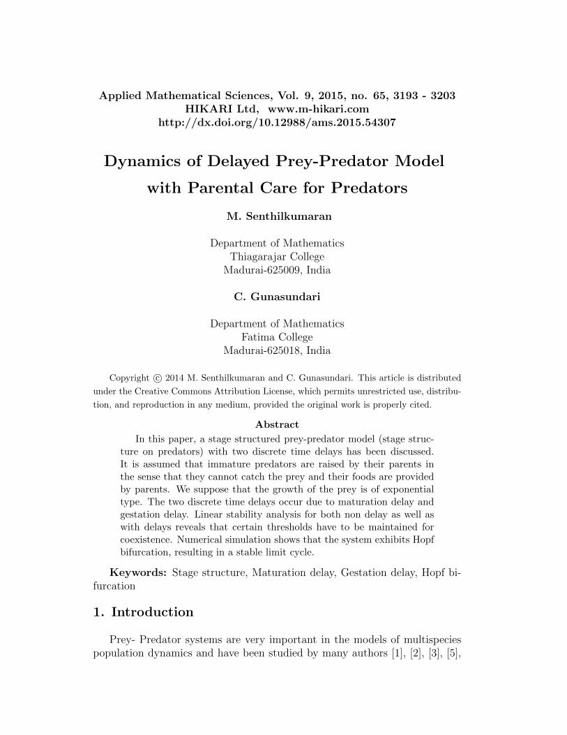
Applied Mathematical Sciences, Vol. 9, 2015, no. 65, 3193 - 3203HIKARI Ltd, www.m-hikari.com

http://dx.doi.org/10.12988/ams.2015.54307

Dynamics of Delayed Prey-Predator Model

with Parental Care for Predators

M. Senthilkumaran

Department of MathematicsThiagarajar College

Madurai-625009, India

C. Gunasundari

Department of MathematicsFatima College

Madurai-625018, India

Copyright c© 2014 M. Senthilkumaran and C. Gunasundari. This article is distributed

under the Creative Commons Attribution License, which permits unrestricted use, distribu-

tion, and reproduction in any medium, provided the original work is properly cited.

Abstract

In this paper, a stage structured prey-predator model (stage struc-ture on predators) with two discrete time delays has been discussed.It is assumed that immature predators are raised by their parents inthe sense that they cannot catch the prey and their foods are providedby parents. We suppose that the growth of the prey is of exponentialtype. The two discrete time delays occur due to maturation delay andgestation delay. Linear stability analysis for both non delay as well aswith delays reveals that certain thresholds have to be maintained forcoexistence. Numerical simulation shows that the system exhibits Hopfbifurcation, resulting in a stable limit cycle.

Keywords: Stage structure, Maturation delay, Gestation delay, Hopf bi-furcation

1. Introduction

Prey- Predator systems are very important in the models of multispeciespopulation dynamics and have been studied by many authors [1], [2], [3], [5],

3194 M. Senthilkumaran and C. Gunasundari

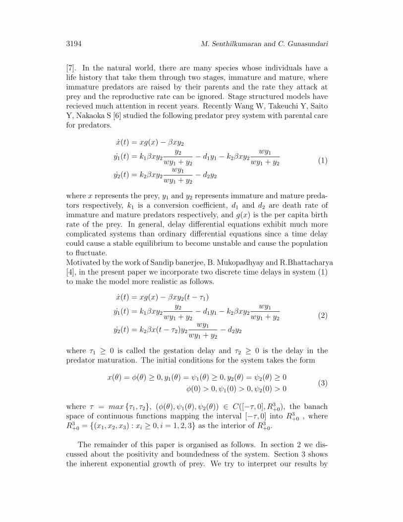
[7]. In the natural world, there are many species whose individuals have alife history that take them through two stages, immature and mature, whereimmature predators are raised by their parents and the rate they attack atprey and the reproductive rate can be ignored. Stage structured models haverecieved much attention in recent years. Recently Wang W, Takeuchi Y, SaitoY, Nakaoka S [6] studied the following predator prey system with parental carefor predators.

x(t) = xg(x)− βxy2y1(t) = k1βxy2

y2wy1 + y2

− d1y1 − k2βxy2wy1

wy1 + y2

y2(t) = k2βxy2wy1

wy1 + y2− d2y2

(1)

where x represents the prey, y1 and y2 represents immature and mature preda-tors respectively, k1 is a conversion coefficient, d1 and d2 are death rate ofimmature and mature predators respectively, and g(x) is the per capita birthrate of the prey. In general, delay differential equations exhibit much morecomplicated systems than ordinary differential equations since a time delaycould cause a stable equilibrium to become unstable and cause the populationto fluctuate.Motivated by the work of Sandip banerjee, B. Mukopadhyay and R.Bhattacharya[4], in the present paper we incorporate two discrete time delays in system (1)to make the model more realistic as follows.

x(t) = xg(x)− βxy2(t− τ1)

y1(t) = k1βxy2y2

wy1 + y2− d1y1 − k2βxy2

wy1wy1 + y2

y2(t) = k2βx(t− τ2)y2wy1

wy1 + y2− d2y2

(2)

where τ1 ≥ 0 is called the gestation delay and τ2 ≥ 0 is the delay in thepredator maturation. The initial conditions for the system takes the form

x(θ) = φ(θ) ≥ 0, y1(θ) = ψ1(θ) ≥ 0, y2(θ) = ψ2(θ) ≥ 0

φ(0) > 0, ψ1(0) > 0, ψ2(0) > 0(3)

where τ = max τ1, τ2, (φ(θ), ψ1(θ), ψ2(θ)) ∈ C([−τ, 0], R3+0), the banach

space of continuous functions mapping the interval [−τ, 0] into R3+0 , where

R3+0 = (x1, x2, x3) : xi ≥ 0, i = 1, 2, 3 as the interior of R3

+0.

The remainder of this paper is organised as follows. In section 2 we dis-cussed about the positivity and boundedness of the system. Section 3 showsthe inherent exponential growth of prey. We try to interpret our results by

Dynamics of delayed prey-predator model 3195

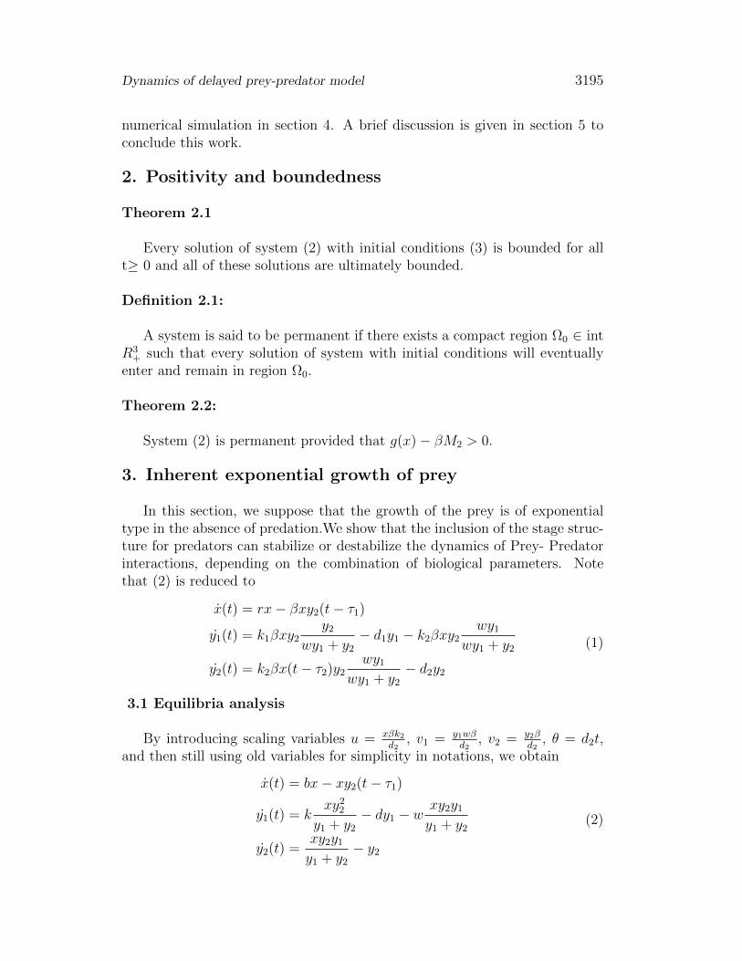
numerical simulation in section 4. A brief discussion is given in section 5 toconclude this work.

2. Positivity and boundedness

Theorem 2.1

Every solution of system (2) with initial conditions (3) is bounded for allt≥ 0 and all of these solutions are ultimately bounded.

Definition 2.1:

A system is said to be permanent if there exists a compact region Ω0 ∈ intR3

+ such that every solution of system with initial conditions will eventuallyenter and remain in region Ω0.

Theorem 2.2:

System (2) is permanent provided that g(x)− βM2 > 0.

3. Inherent exponential growth of prey

In this section, we suppose that the growth of the prey is of exponentialtype in the absence of predation.We show that the inclusion of the stage struc-ture for predators can stabilize or destabilize the dynamics of Prey- Predatorinteractions, depending on the combination of biological parameters. Notethat (2) is reduced to

x(t) = rx− βxy2(t− τ1)

y1(t) = k1βxy2y2

wy1 + y2− d1y1 − k2βxy2

wy1wy1 + y2

y2(t) = k2βx(t− τ2)y2wy1

wy1 + y2− d2y2

(1)

3.1 Equilibria analysis

By introducing scaling variables u = xβk2d2

, v1 = y1wβd2

, v2 = y2βd2

, θ = d2t,and then still using old variables for simplicity in notations, we obtain

x(t) = bx− xy2(t− τ1)

y1(t) = kxy22

y1 + y2− dy1 − w

xy2y1y1 + y2

y2(t) =xy2y1y1 + y2

− y2

(2)


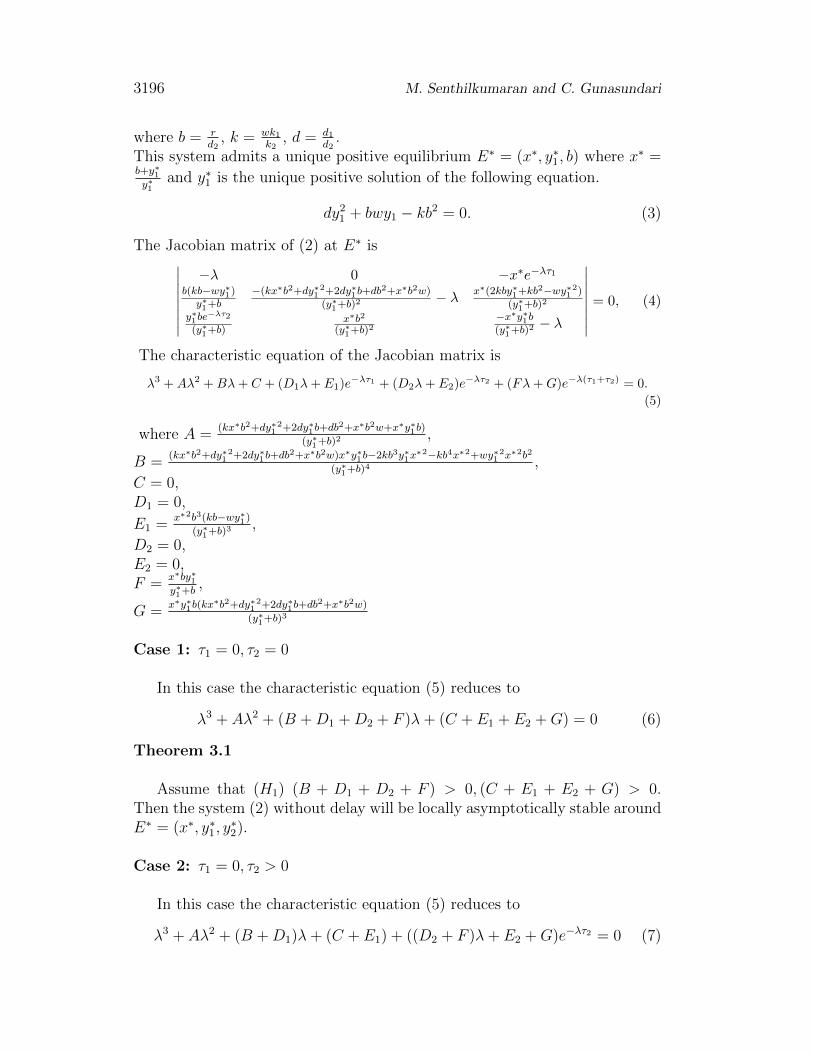
where b = rd2

, k = wk1k2

, d = d1d2

.This system admits a unique positive equilibrium E∗ = (x∗, y∗1, b) where x∗ =b+y∗1y∗1

and y∗1 is the unique positive solution of the following equation.

dy21 + bwy1 − kb2 = 0. (3)

The Jacobian matrix of (2) at E∗ is∣∣∣∣∣∣∣∣−λ 0 −x∗e−λτ1

b(kb−wy∗1)y∗1+b

−(kx∗b2+dy∗12+2dy∗1b+db

2+x∗b2w)(y∗1+b)

2 − λ x∗(2kby∗1+kb2−wy∗1

2)(y∗1+b)

2

y∗1be−λτ2

(y∗1+b)x∗b2

(y∗1+b)2

−x∗y∗1b(y∗1+b)

2 − λ

∣∣∣∣∣∣∣∣ = 0, (4)

The characteristic equation of the Jacobian matrix is

λ3 +Aλ2 +Bλ+ C + (D1λ+ E1)e−λτ1 + (D2λ+ E2)e

−λτ2 + (Fλ+G)e−λ(τ1+τ2) = 0.

(5)

where A =(kx∗b2+dy∗1

2+2dy∗1b+db2+x∗b2w+x∗y∗1b)

(y∗1+b)2 ,

B =(kx∗b2+dy∗1

2+2dy∗1b+db2+x∗b2w)x∗y∗1b−2kb3y∗1x∗

2−kb4x∗2+wy∗12x∗2b2

(y∗1+b)4 ,

C = 0,D1 = 0,

E1 =x∗2b3(kb−wy∗1)

(y∗1+b)3 ,

D2 = 0,E2 = 0,F =

x∗by∗1y∗1+b

,

G =x∗y∗1b(kx

∗b2+dy∗12+2dy∗1b+db

2+x∗b2w)

(y∗1+b)3

Case 1: τ1 = 0, τ2 = 0

In this case the characteristic equation (5) reduces to

λ3 + Aλ2 + (B +D1 +D2 + F )λ+ (C + E1 + E2 +G) = 0 (6)

Theorem 3.1

Assume that (H1) (B + D1 + D2 + F ) > 0, (C + E1 + E2 + G) > 0.Then the system (2) without delay will be locally asymptotically stable aroundE∗ = (x∗, y∗1, y

∗2).

Case 2: τ1 = 0, τ2 > 0


λ3 + Aλ2 + (B +D1)λ+ (C + E1) + ((D2 + F )λ+ E2 +G)e−λτ2 = 0 (7)


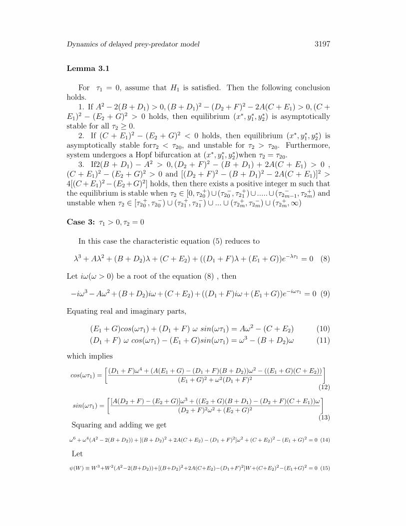
Lemma 3.1

For τ1 = 0, assume that H1 is satisfied. Then the following conclusionholds.

1. If A2 − 2(B +D1) > 0, (B +D1)2 − (D2 + F )2 − 2A(C +E1) > 0, (C +

E1)2 − (E2 + G)2 > 0 holds, then equilibrium (x∗, y∗1, y

∗2) is asymptotically

stable for all τ2 ≥ 0.2. If (C + E1)

2 − (E2 + G)2 < 0 holds, then equilibrium (x∗, y∗1, y∗2) is

asymptotically stable forτ2 < τ20, and unstable for τ2 > τ20. Furthermore,system undergoes a Hopf bifurcation at (x∗, y∗1, y

∗2)when τ2 = τ20.

3. If2(B + D1) − A2 > 0, (D2 + F )2 − (B + D1) + 2A(C + E1) > 0 ,(C + E1)

2 − (E2 + G)2 > 0 and [(D2 + F )2 − (B + D1)2 − 2A(C + E1)]

2 >4[(C+E1)

2− (E2 +G)2] holds, then there exists a positive integer m such thatthe equilibrium is stable when τ2 ∈ [0, τ2

+0 )∪ (τ2

−0 , τ2

+1 )∪ .....∪ (τ2

−m−1, τ2

+m) and

unstable when τ2 ∈ [τ2+0 , τ2

−0 ) ∪ (τ2

+1 , τ2

−1 ) ∪ ... ∪ (τ2

+m, τ2

−m) ∪ (τ2

+m,∞)

Case 3: τ1 > 0, τ2 = 0


λ3 + Aλ2 + (B +D2)λ+ (C + E2) + ((D1 + F )λ+ (E1 +G))e−λτ1 = 0 (8)

Let iω(ω > 0) be a root of the equation (8) , then

−iω3−Aω2 +(B+D2)iω+(C+E2)+((D1 +F )iω+(E1 +G))e−iωτ1 = 0 (9)

Equating real and imaginary parts,

(E1 +G)cos(ωτ1) + (D1 + F ) ω sin(ωτ1) = Aω2 − (C + E2) (10)

(D1 + F ) ω cos(ωτ1)− (E1 +G)sin(ωτ1) = ω3 − (B +D2)ω (11)

which implies

cos(ωτ1) =

[(D1 + F )ω4 + (A(E1 +G)− (D1 + F )(B +D2))ω

2 − ((E1 +G)(C + E2))

(E1 +G)2 + ω2(D1 + F )2

](12)

sin(ωτ1) =

[[A(D2 + F )− (E2 +G)]ω3 + ((E2 +G)(B +D1)− (D2 + F )(C + E1))ω

(D2 + F )2ω2 + (E2 +G)2

](13)

Squaring and adding we get

ω6 + ω4(A2 − 2(B +D2)) + [(B +D2)2 + 2A(C +E2)− (D1 + F )2]ω2 + (C +E2)

2 − (E1 +G)2 = 0 (14)

Let

ψ(W ) ≡W 3+W 2(A2−2(B+D2))+[(B+D2)2+2A(C+E2)−(D1+F )2]W+(C+E2)

2−(E1+G)2 = 0 (15)


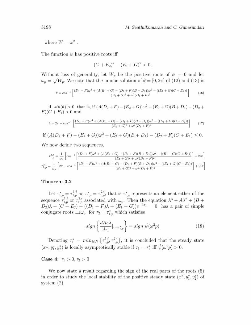
where W = ω2 .

The function ψ has positive roots iff

(C + E2)2 − (E1 +G)2 < 0,

Without loss of generality, let Wp be the positive roots of ψ = 0 and letωp =

√Wp. We note that the unique solution of θ = [0, 2π] of (12) and (13) is

θ = cos−1

[(D1 + F )ω4 + (A(E1 +G)− (D1 + F )(B +D2))ω2 − ((E1 +G)(C + E2))

(E1 +G)2 + ω2(D1 + F )2

](16)

if sin(θ) > 0, that is, if (A(D2+F )− (E2+G))ω2+(E2+G)(B+D1)− (D2+F )(C + E1) > 0 and

θ = 2π − cos−1


(E1 +G)2 + ω2(D1 + F )2

](17)

if (A(D2 + F )− (E2 +G))ω2 + (E2 +G)(B +D1)− (D2 + F )(C + E1) ≤ 0.

We now define two sequences,

τ1,i1,p =1

ωp

[cos−1


(E1 +G)2 + ω2(D1 + F )2

]+ 2iπ

]τ2,i1,p =

1

ωp

[2π − cos−1


(E1 +G)2 + ω2(D1 + F )2

]+ 2iπ

]

Theorem 3.2

Let τ ∗1,p = τ 1,i1,p or τ∗1,p = τ 2,i1,p, that is τ ∗1,p represents an element either of the

sequence τ 1,i1,p or τ 2,i1,p associated with ωp. Then the equation λ3 + Aλ2 + (B +D2)λ + (C + E2) + ((D1 + F )λ + (E1 + G))e−λτ1 = 0 has a pair of simpleconjugate roots ±iωp for τ2 = τ ∗1,p which satisfies

sign

dReλ

dτ1|τ=τ∗1,p

= sign ψ(ω2p) (18)

Denoting τ ∗1 = mini∈Nτ 1,i1,p, τ

2,i1,p

, it is concluded that the steady state

(x∗, y∗1, y∗2) is locally asymptotically stable if τ1 = τ ∗1 iff ψ(ω2p) > 0.

Case 4: τ1 > 0, τ2 > 0

We now state a result regarding the sign of the real parts of the roots (5)in order to study the local stability of the positive steady state (x∗, y∗1, y

∗2) of

system (2).


Proposition (P1):

If all the roots of the equation (5) have negative real parts for some τ1 > 0,then there exists a τ ∗2 (τ1) > 0 such that all the roots of equation (5) (i.e withτ2 > 0) have negative real parts when τ2 < τ ∗2 (τ1) .

Considering the above proposition we can now state the following theorem.

Theorem 3.3

If we assume that the hypothesis P1 hold, then for any τ1 ∈ [0, τ ∗1 ), thereexists a τ ∗2 (τ1) > 0 such that the positive steady state (x∗, y∗1, y

∗2) of the sytem

is locally asymptotically stable when τ1 ∈ [0, τ ∗1 ).

Proof:

Using the above theorem, we can say that all the roots of (5) have negativereal parts when τ1 ∈ [0, τ ∗1 ) and by proposition we can conclude that thereexists a τ ∗2 (τ1) > 0 such that all the roots of equation (5) have negative realparts when τ2 < τ ∗2 (τ1) . Hence the steady state (x∗, y∗1, y

∗2) of system (2) is

locally asymptotically stable when τ1 ∈ [0, τ ∗1 ).

4. Numerical Simulation

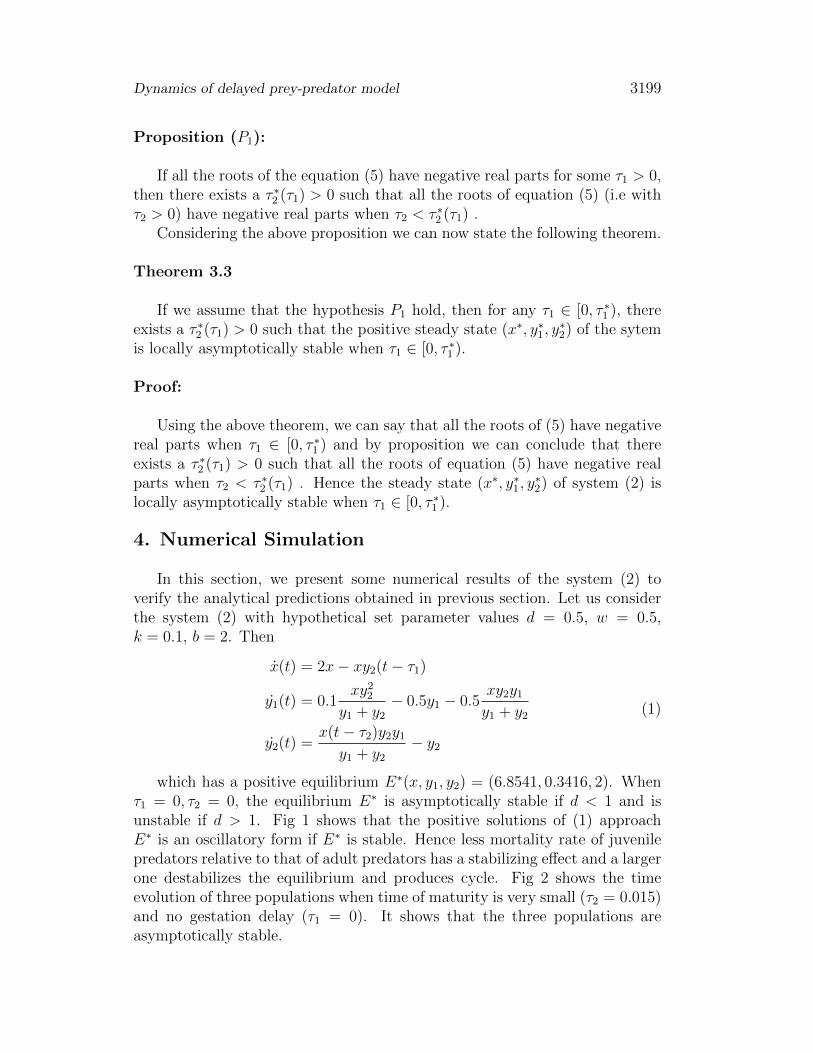
In this section, we present some numerical results of the system (2) toverify the analytical predictions obtained in previous section. Let us considerthe system (2) with hypothetical set parameter values d = 0.5, w = 0.5,k = 0.1, b = 2. Then

x(t) = 2x− xy2(t− τ1)

y1(t) = 0.1xy22

y1 + y2− 0.5y1 − 0.5

xy2y1y1 + y2

y2(t) =x(t− τ2)y2y1y1 + y2

− y2

(1)

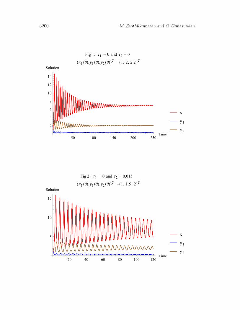
which has a positive equilibrium E∗(x, y1, y2) = (6.8541, 0.3416, 2). Whenτ1 = 0, τ2 = 0, the equilibrium E∗ is asymptotically stable if d < 1 and isunstable if d > 1. Fig 1 shows that the positive solutions of (1) approachE∗ is an oscillatory form if E∗ is stable. Hence less mortality rate of juvenilepredators relative to that of adult predators has a stabilizing effect and a largerone destabilizes the equilibrium and produces cycle. Fig 2 shows the timeevolution of three populations when time of maturity is very small (τ2 = 0.015)and no gestation delay (τ1 = 0). It shows that the three populations areasymptotically stable.


50 100 150 200 250Time

2

4

6

8

10

12

14

Solution

x

y1

y2

Fig 1: Τ1 = 0 and Τ2 = 0

H x1 HΘL,y1 HΘL,y2 HΘLLT =H1, 2, 2.2 LT

20 40 60 80 100 120Time

5

10

15

Solution

x

y1

y2

Fig 2: Τ1 = 0 and Τ2 = 0.015

H x1 HΘL,y1 HΘL,y2 HΘLLT =H1, 1.5 , 2LT


20 40 60 80 100Time

2

4

6

8

10

12

14

Solution

x

y1

y2

Fig 3: Τ1 = 0.012 and Τ2 = 0

H x1 HΘL,y1 HΘL,y2 HΘLLT =H1, 1.7 , 2.1 LT

20 40 60 80Time

5

10

15

Solution

x

y1

y2

Fig 4: Τ1 = 0.013 and Τ2 = 0.01

H x1 HΘL,y1 HΘL,y2 HΘLLT =H1, 1.8 , 2.2 LT


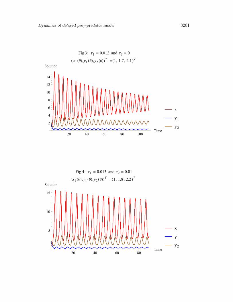
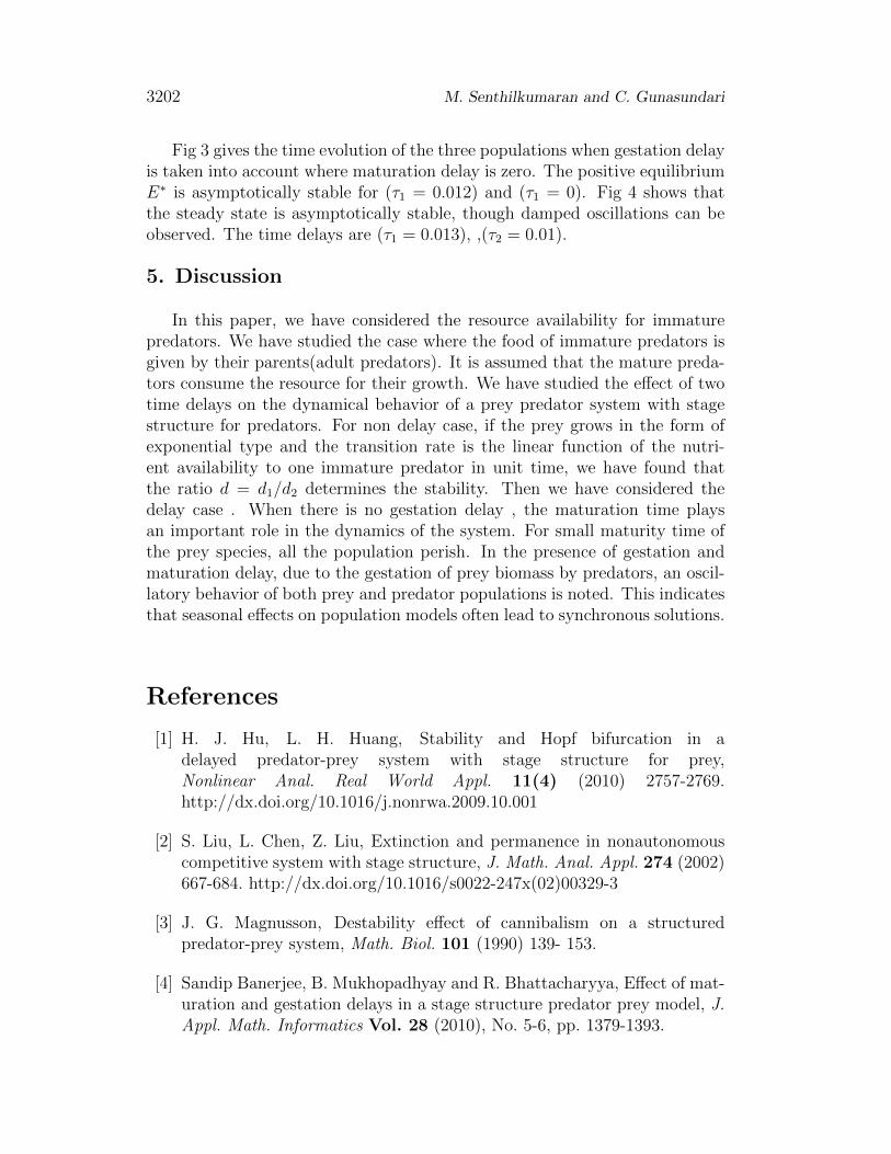
Fig 3 gives the time evolution of the three populations when gestation delayis taken into account where maturation delay is zero. The positive equilibriumE∗ is asymptotically stable for (τ1 = 0.012) and (τ1 = 0). Fig 4 shows thatthe steady state is asymptotically stable, though damped oscillations can beobserved. The time delays are (τ1 = 0.013), ,(τ2 = 0.01).

5. Discussion

In this paper, we have considered the resource availability for immaturepredators. We have studied the case where the food of immature predators isgiven by their parents(adult predators). It is assumed that the mature preda-tors consume the resource for their growth. We have studied the effect of twotime delays on the dynamical behavior of a prey predator system with stagestructure for predators. For non delay case, if the prey grows in the form ofexponential type and the transition rate is the linear function of the nutri-ent availability to one immature predator in unit time, we have found thatthe ratio d = d1/d2 determines the stability. Then we have considered thedelay case . When there is no gestation delay , the maturation time playsan important role in the dynamics of the system. For small maturity time ofthe prey species, all the population perish. In the presence of gestation andmaturation delay, due to the gestation of prey biomass by predators, an oscil-latory behavior of both prey and predator populations is noted. This indicatesthat seasonal effects on population models often lead to synchronous solutions.

References

[1] H. J. Hu, L. H. Huang, Stability and Hopf bifurcation in adelayed predator-prey system with stage structure for prey,Nonlinear Anal. Real World Appl. 11(4) (2010) 2757-2769.http://dx.doi.org/10.1016/j.nonrwa.2009.10.001

[2] S. Liu, L. Chen, Z. Liu, Extinction and permanence in nonautonomouscompetitive system with stage structure, J. Math. Anal. Appl. 274 (2002)667-684. http://dx.doi.org/10.1016/s0022-247x(02)00329-3

[3] J. G. Magnusson, Destability effect of cannibalism on a structuredpredator-prey system, Math. Biol. 101 (1990) 139- 153.

[4] Sandip Banerjee, B. Mukhopadhyay and R. Bhattacharyya, Effect of mat-uration and gestation delays in a stage structure predator prey model, J.Appl. Math. Informatics Vol. 28 (2010), No. 5-6, pp. 1379-1393.


[5] W. Wang, G. Mulone, F. Salemi, V. Salone, Permanence and stabilityof a stage-structured predator-prey model, J. Math. Anal. Appl. 262 (2)(2001) 499-528. http://dx.doi.org/10.1006/jmaa.2001.7543

[6] W. Wang, Y. Takeuchi, Y. Saito, S. Nakaoka, Prey-Predator system withparental care for predators, J Theor Biol. 2006 Aug 7; 241(3): 451-8.Epub 2006 jan 18. http://dx.doi.org/10.1016/j.jtbi.2005.12.008

[7] F. Wei, K. Wang, Permanence of variable coefficients predator-preysystem with stage structure,Appl.Math.Comput. 180 (2006) 594-598.http://dx.doi.org/10.1016/j.amc.2005.12.062

Received: December 15, 2014; Published: April 20, 2015

Documents

Dynamics of Delayed Prey-Predator Model with Parental …m-hikari.com/.../ams-65-68-2015/p/01gunasundariAMS65-68-2015-26.pdf · Dynamics of delayed prey-predator model 3195 numerical