Dynamics of continuous-time quantum walks in restricted geometries

This article has been downloaded from IOPscience. Please scroll down to see the full text article.

2008 J. Phys. A: Math. Theor. 41 445301

(http://iopscience.iop.org/1751-8121/41/44/445301)

Download details:

IP Address: 160.78.34.140

The article was downloaded on 13/11/2008 at 10:34

Please note that terms and conditions apply.

The Table of Contents and more related content is available

HOME | SEARCH | PACS & MSC | JOURNALS | ABOUT | CONTACT US

IOP PUBLISHING JOURNAL OF PHYSICS A: MATHEMATICAL AND THEORETICAL

J. Phys. A: Math. Theor. 41 (2008) 445301 (21pp) doi:10.1088/1751-8113/41/44/445301

Dynamics of continuous-time quantum walks inrestricted geometries

E Agliari, A Blumen and O Mulken

Theoretische Polymerphysik, Universitat Freiburg, Hermann-Herder-Str. 3, D-79104 Freiburg,Germany

Received 19 July 2008, in final form 4 September 2008Published 7 October 2008Online at stacks.iop.org/JPhysA/41/445301

Abstract

We study quantum transport on finite discrete structures and we model theprocess by means of continuous-time quantum walks. A direct and effectivecomparison between quantum and classical walks can be attained based onthe average displacement of the walker as a function of time. Indeed, afast growth of the average displacement can be advantageously exploited tobuild up efficient search algorithms. By means of analytical and numericalinvestigations, we show that the finiteness and the inhomogeneity of thesubstrate jointly weaken the quantum-walk performance. We further highlightthe interplay between the quantum-walk dynamics and the underlying topologyby studying the temporal evolution of the transfer probability distribution andthe lower bound of long-time averages.

PACS numbers: 05.60.Gg, 71.35.−y, 05.60.Cd

(Some figures in this article are in colour only in the electronic version)

1. Introduction

Quantum walks (QWs) are attracting increasing attention in many research areas, rangingfrom solid-state physics to quantum computing [1]. In particular, QWs provide a model forquantum-mechanical transport processes on discrete structures; this includes, for instance, thecoherent energy transfer of a qubit on an optical lattice [2–5]. The theoretical study of QWsis also encouraged by recent experimental implementations able to corroborate theoreticalfindings [6–8].

As in the classical random walk, quantum walks appear in a discrete [9] as well as in acontinuous-time (CTQW) [10] form; these forms, however, cannot be simply related to eachother [11]. Now, standard CTQWs, on which we focus, can be obtained by identifying theHamiltonian of the system with the classical transfer matrix which is, in turn, directly relatedto the Laplacian of the underlying structure.

1751-8113/08/445301+21$30.00 © 2008 IOP Publishing Ltd Printed in the UK 1

J. Phys. A: Math. Theor. 41 (2008) 445301 E Agliari et al

Another feature which CTQWs share with classical random walks consists of the stronginterplay between the dynamics properties displayed by the walk and the topology of thesubstrate [12–14]. However, the dependences turn out to be much more complex in thequantum-mechanical case: while the classical (simple) walk eventually loses memory of itsstarting site, the quantum walk exhibits, even in the asymptotic regime, transition probabilitieswhich depend on the starting site. For this reason, often the parameters describing the transportare averaged over all initial sites, a procedure which allows a global characterization of thewalk, while preserving its most important features.

One of the quantities affected by topology is the mean-square displacement of thewalker up to time t. Classically, this quantity is monotonically increasing and depends(asymptotically) on time according to the power law 〈r2(t)〉 ∼ tβ . The value of the ‘diffusionexponent’ β allows us to distinguish between normal (β = 1) and anomalous (β �= 1) diffusion[15]. As for quantum transport, it is possible to introduce analogous exponents, characterizingthe temporal spreading of a wave packet [16]. However, even when they take place over thesame structure, quantum and classical walks can exhibit dramatically different behaviours. Inparticular, the quantum wave propagation on regular, infinite lattices is ballistic, i.e. the root-mean-square displacement is linear in time. Such a quadratic speed-up of the mean-squaredisplacement is a well-known phenomenon when dealing with tight-binding electron waveson periodic lattices [9] and, from a computational point of view, it constitutes an importantfeature since it could be advantageously exploited in quantum search algorithms [17–19]. Inthe presence of disorder (either deterministic or stochastic) or finiteness, the sharp ballisticfronts are softened, a fact which may even lead to the localization of the quantum particle[20, 21]. It is therefore of both theoretical and practical interest to highlight how finitenessand inhomogeneity—often unavoidable in real systems—affect the particle’s propagation. Tothis aim we analyse quantum transport on restricted geometries, where the restrictions arisefrom the (possibly joint) fractal dimension and finite extent of the substrate itself. By directcomparison with the classical case, we find that, on finite substrates, the advantage of CTQWsis at short times only. Moreover, the lack of translational invariance weakens the CTQWperformance, i.e. in such situations the average displacement increases more slowly withtime.

The finite discrete structures we consider and compare are the dual Sierpinski gasket(DSG), the Cayley tree (CT) vide infra section 4 and the square lattice with periodic boundaryconditions, i.e. the square torus (ST). These constitute representative topologies, providingexamples of fractals with loops, of trees and of regular structures. The dual Sierpinski gasketwill be treated in more detail; for this structure the eigenvalue spectrum of the Laplacianmatrix is known exactly, allowing for some analytical estimates. Indeed, not only randomwalks, but also many dynamical properties of connected structures themselves (such as thevibrational structures and the relaxation modes) depend on the spectrum of their Laplacianmatrix [22]. However, for CTQWs the set of eigenvectors also matters, which often makesanalytical investigations cumbersome.

It is worth underlining that focusing on discrete structures is not only suggested by solid-state applications: quantum computation is traditionally concerned with the manipulation ofdiscrete systems. In particular, a discrete (and finite) state space makes the CTQW simulationby quantum computers, working with discrete registers, feasible [1, 23].

Our paper is structured as follows. After a brief summary of the main concepts andof the formulae concerning CTQWs in section 2, we describe the topology of the DSG insection 3. Then, in section 4, we study the quantum-mechanical transport over the above-mentioned structures, especially focusing on the average displacement and on the long-timeaverages. Finally, in section 5 we present our comments and conclusions. In the appendix,

2

J. Phys. A: Math. Theor. 41 (2008) 445301 E Agliari et al

we derive analytical results concerning the average chemical displacements of CTQWs overhypercubic lattices, special cases being chains and square lattices.

2. Continuous-time quantum walks on graphs

Mathematically, a graph is specified by the pair {V,E} consisting of a nonempty, countableset of points V , joined pairwise by a set of links E. The cardinality of V provides the numberN of sites making up the graph, i.e. its volume: |V | = N . In the following, we focus mainlyon finite graphs (N < ∞) and we label each node with a lowercase letter i ∈ V .

From an algebraic point of view, a graph can be described by its adjacency matrix A,whose elements are

Aij ={

1, if (i, j) ∈ E,

0, otherwise.

The connectivity of a node i can be calculated as a sum of matrix elements zi = ∑j Aij . The

Laplacian operator is then defined as L = Z − A, where Z is the diagonal matrix given byZik = ziδik .

The Laplacian matrix L is symmetric and non-negative definite and it can thereforegenerate a probability conserving Markov process and define a unitary process as well.Otherwise stated, the Laplacian operator can work both as a classical transfer operator and asa tight-binding Hamiltonian of a quantum transport process [24, 25].

Indeed, the classical continuous-time random walk (CTRW) is described by the followingMaster equation [26]:

d

dtpk,j (t) =

N∑l=1

Tklpl,j (t), (1)

where pk,j (t) is the conditional probability that the walker is on node k when it started fromnode j at time 0. If the walk is symmetric with a site-independent transmission rate γ , thenthe transfer matrix T is simply related to the Laplacian operator through T = −γ L.

Now the CTQW, the quantum-mechanical counterpart of the CTRW, is introduced byidentifying the Hamiltonian of the system with the classical transfer matrix, H = −T

[10, 13, 24] (in the following we will set h ≡ 1). The set of states |j 〉, representing thewalker localized at the node j , spans the whole accessible Hilbert space and also providesan orthonormal basis set. Therefore, the behaviour of the walker can be described by thetransition amplitude αk,j (t) from state |j 〉 to state |k〉, which obeys the following Schrodingerequation:

d

dtαk,j (t) = −i

N∑l=1

Hklαl,j (t). (2)

If at the initial time t0 = 0 only the state |j 〉 is populated, then the formal solution toequation (2) can be written as

αk,j (t) = 〈k| exp(−iHt)|j 〉, (3)

whose squared magnitude provides the quantum-mechanical transition probability πk,j (t) ≡|αk,j (t)|2. In general, it is convenient to introduce the orthonormal basis |ψn〉, n ∈ [1,N ]which diagonalizes T (and, clearly, also H); the correspondent set of eigenvalues is denotedby {λn}n=1,...,N . Thus, we can write

πk,j (t) =∣∣∣∣∣

N∑n=1

〈k| e−iλnt |ψn〉〈ψn|j 〉∣∣∣∣∣2

. (4)

3

J. Phys. A: Math. Theor. 41 (2008) 445301 E Agliari et al

Despite the apparent similarity between equations (1) and (2), some important differencesare worth being recalled.

First, the imaginary unit makes the time evolution operator U(t) = exp(−iHt) unitary,which prevents the quantum-mechanical transition probability from having a definite limit ast → ∞. On the other hand, a particle performing a CTRW is asymptotically equally likely tobe found on any site of the structure: the classical pk,j (t) admit a stationary distribution whichis independent of initial and final sites, limt→∞ pk,j (t) = 1/N . Hence, in order to compareclassical long-time probabilities with quantum-mechanical ones, we rely on the long-timeaverage (LTA) [27], defined in section 4.4.

Moreover, the normalization conditions for pk,j (t) and αk,j (t) read∑N

k=1 pk,j (t) = 1 and∑Nk=1 |αk,j (t)|2 = 1.

2.1. Average displacement

The average displacement performed by a quantum walker until time t allows a straightforwardcomparison with the classical case; it is also more directly related to transport properties thanthe transfer probability πk,j (t): it constitutes the expectation value of the distance reached bythe particle after a time t and its time dependence provides information on how fast the particlepropagates over the substrate.

For CTQW (subscript q) starting at node j , we define the average (chemical) displacement〈rj (t)〉q performed until time t as

〈rj (t)〉q =N∑

k=1

(k, j)πk,j (t), (5)

where (k, j) is the chemical distance between the sites j and k, i.e. the length of the shortestpath connecting j and k. We can average over all starting points to obtain

〈r(t)〉q = 1

N

N∑j=1

〈rj (t)〉q . (6)

For fractals or hyperbranched structures it is more appropriate to use the chemical distance,rather than the Euclidean distance; for instance, the infinite CT (see section 4) cannot beembedded in any lattice of finite dimension. For classical diffusion, it is well known that thechemical and the Euclidean distances display analogous asymptotic laws for regular structuresand for many deterministic fractals (e.g. the Sierpinski gasket) [15]; as discussed in theappendix, this still holds for CTQWs on arbitrary d-dimensional hypercubic lattices.

For classical (subscript c) regular diffusion (on infinite lattices) the average displacement〈r(t)〉c depends on time t according to

〈r(t)〉c ∼ t1/2. (7)

More generally, for scaling (fractal) structures we can define the so-called chemical diffusionexponent d

w and get [15]:

〈r(t)〉c ∼ t1/dw . (8)

Finite systems require corrections to these laws: for them 〈r(t)〉c does not grow indefinitely,but it saturates to a maximum value rc [28].

4

J. Phys. A: Math. Theor. 41 (2008) 445301 E Agliari et al

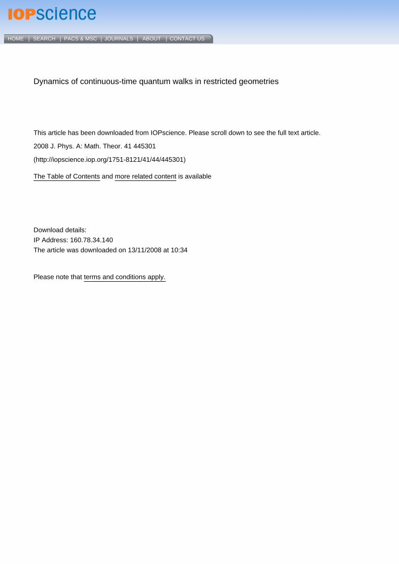
2.2. Return probability

As is well known, for a diffusive particle the probability to return to the starting point istopology sensitive and it can indeed be used to extract information about the underlyingstructure [26]. It is therefore interesting to compare the classical return probability pk,k(t)

with the quantum-mechanical πk,k(t) (see also [29, 30]). One has

pk,k(t) = 〈k| exp(Tt)|k〉 =N∑

n=1

|〈k|ψn〉|2 exp(−γ tλn) (9)

and

πk,k(t) = ∣∣αk,k(t)∣∣2 =

∣∣∣∣∣N∑

n=1

|〈k|ψn〉|2 exp(−iγ tλn)

∣∣∣∣∣2

. (10)

In order to get a global information about the likelihood to be (return or stay) at the origin,independent of the starting site, we average over all sites of the graph, obtaining

p(t) = 1

N

N∑k=1

pk,k(t) = 1

N

N∑n=1

e−γ λnt (11)

and

π(t) = 1

N

N∑k=1

πk,k(t) = 1

N

N∑n,m=1

e−iγ (λn−λm)t

N∑k=1

|〈k|ψn〉|2 |〈k|ψm〉|2 . (12)

For finite substrates, the classical p(t) decays monotonically to the equipartition limit, andit only depends on the eigenvalues of T. On the other hand, π(t) depends explicitly on theeigenvectors of H [29, 30]. By means of the Cauchy–Schwarz inequality we can obtain alower bound for π(t) which does not depend on the eigenvectors [30, 31]:

π(t) �∣∣∣∣∣ 1

N

N∑k=1

αk,k(t)

∣∣∣∣∣ ≡ |α(t)|2 = 1

N 2

N∑m,n=1

e−iγ (λn−λm)t . (13)

Note that equations (11) and (12) can serve as measures of the efficiency of the transport processperformed by CTRW and CTQW, respectively. In fact, the faster p(t) decreases towards itsasymptotic value, the more efficient the transport. Analogously, a more rapid decay of theenvelope of π(t) (or of |α(t)|2) implies a faster delocalization of the quantum walker overthe graph. By the way, we recall that, for a large variety of graphs [30], the classical averagereturn probability scales as p(t) ∼ t−μ, while the envelope of |α(t)|2, namely env[|α(t)|2],scales like t−2μ, μ being a proper parameter related for fractals to the spectral density.

As can be inferred by comparing equations (11) and (12), for quantum transport processesthe degeneracy of the eigenvalues plays an important role, as the differences betweeneigenvalues determine the temporal behaviour, while for classical transport the long-timebehaviour is dominated by the smallest eigenvalue. Situations in which only a few, highlydegenerate eigenvalues are present are related to slow CTQW dynamics, while when alleigenvalues are non-degenerate the transport turns out to be efficient [29, 30].

3. Dual Sierpinski gasket: topology and eigenvalue spectrum

Before turning to the dynamics of CTQW (and CTRW) on exemplary structures, which allowus to highlight the importance of inhomogeneities, some remarks on the spectra of the DSGare in order.

5

J. Phys. A: Math. Theor. 41 (2008) 445301 E Agliari et al

Figure 1. Dual transformation from Sierpinski gasket to dual Sierpinski gasket of generationg = 3.

The dual Sierpinski gasket is an exactly-decimable fractal which is directly related,through a dual transformation, to the Sierpinski gasket (SG). The DSG of generation g canbe constructed by replacing each small triangle belonging to the SG with a node and byconnecting such nodes whenever the relevant triangles share a vertex in the original gasket(see figure 1). It is straightforward to verify that the number of nodes at any given generationg is N = 3g .

The dual transformation does not conserve the coordination number of the inner nodes(which decreases from 4 to 3), but it does conserve the fractal dimension df and thespectral dimension d , which are therefore the same as for the original Sierpinski gasketdf = ln 3/ ln 2 = 1.58496 . . . and d = 2 ln 3/ ln 5 = 1.36521 . . . .

As mentioned above, the knowledge of the eigenvalue spectrum is sufficient for thecalculation of several interesting quantities concerning the dynamics of CTQWs. In general,any (finite) Hamiltonian H can be (at least numerically) diagonalized in order to obtain itsspectrum. However, as the size of H gets large, the procedure gets to be time consuming and theprecise numerical diagonalization may not be easy to perform. Remarkably, the eigenvaluespectrum of the DSG Laplacian matrix can be determined at any generation through thefollowing iterative procedure; for more details we refer to [34, 35]: at any given generation g

the spectrum includes the non-degenerate eigenvalue λN = 0, the eigenvalue 3 with degeneracy(3g−1+3)/2 and the eigenvalue 5 with degeneracy (3g−1−1)/2. Moreover, given the eigenvaluespectrum at generation g − 1, each non-vanishing eigenvalue λg−1 corresponds to two neweigenvalues λ±

g according to

λ±g = 5 ± √

25 − 4λg−1

2; (14)

both λ+g and λ−

g inherit the degeneracy of λg−1. The eigenvalue spectra is therefore boundedin [0, 5]. As explained in [34], at any generation g, we can calculate the degeneracy of eachdistinct eigenvalue: apart from λN whose degeneracy is 1, there are 2r distinct eigenvalues,each with degeneracy (3g−r−1 + 3)/2, being r = 0, 1, . . . , g − 1, and 2r distinct eigenvalues,each with degeneracy (3g−r−1 − 1)/2, being r = 0, 1, . . . , g − 2. As can be easily verified,the degeneracies sum up to N = 3g . Finally, note that the distribution of eigenvalues and theirdegeneracies are non-uniform and that the spectrum is multifractal [34].

6

J. Phys. A: Math. Theor. 41 (2008) 445301 E Agliari et al

0 5 10 15 200

0.2

0.4

0.6

0.8

1

t(γ−1)

πk

,1(t

)

k = 1k = 2k = 5k = 14

1

2

5

14 18

10

43

79

Figure 2. Exact probability πk,1(t) for the CTQW starting from the apex (site j = 1) to reach sitesk = 1, 2, 5 and 14. The k-sites are the left corners at generations g = 0, 1, 2 and 3, respectively.

4. CTQWs on restricted geometries

4.1. Transfer probability

Results for the exact transition probability distribution πk,j (t) for STs and CTs have alreadybeen given in [13, 31, 32], where it was shown that πk,j (t) depends significantly on the startingnode. The results for ultrametric structures are given in [33].

It is worth recalling here that the Cayley tree (CT) can be built by starting from one node(root) connected to z nodes, which constitute the first shell. Each node of the first shell isthen connected to z − 1 new nodes, which constitute the second shell and so forth, iteratively.Therefore, the Mth shell contains z(z − 1)M−1 nodes which are at a chemical distance M fromthe root. Thus, the CT is a z-regular loop-free graph. The number of sites in a CT of M shellsis NM = [z(z − 1)M − 2]/(z − 2), hence the correlated fractal dimension log(NM)/ log(M)

goes to infinity for M → ∞, precluding the possibility of embedding very large CT in anypreviously specified Euclidean lattice. In the following we focus on finite 3-Cayley trees,which means that z is fixed and equal to three for any internal site of the graph; furthermore,the number of shells (also called generation) is finite (and therefore also the number of nodesis itself finite).

In figure 2 we show our results for a DSG of generation g = 3 and we focus on theset of pairs given by (vn, 1), where vn denotes any of the two corners of the gasket of thenth generation, with n � g (i.e., according to the labelling of figure 2, v0 = 1, v1 = 2,

v2 = 5, v3 = 14). Now, due to the symmetry the DSG is endowed with, for CTQWs startingfrom a given vertex, say the apex, the left and right corners are equivalent. As expected,πk,j (t) does not converge to any definite value, but it displays oscillations whose amplitudesand average values get smaller as the distance between the sites 1 and vn increases. Thissuggests, at least when starting from a main vertex, that the CTQW stays mainly localized atthe origin and its neighbourhood.

7

J. Phys. A: Math. Theor. 41 (2008) 445301 E Agliari et al

0

10

20

0

10

20

0

0.25

0.5

0.75

1

t = 0(γ−1)

kj

πk

,j(t

)

0

10

20

0

10

20

0

0.25

0.5

0.75

1

t = 1(γ−1)

kj

πk

,j(t

)

0

10

20

0

10

20

0

0.25

0.5

0.75

1

t = 3(γ−1)

kj

πk

,j(t

)

0

10

20

0

10

20

0

0.25

0.5

0.75

1

t = 4(γ−1)

kj

πk

,j(t

)

Figure 3. Snapshots of the transition probability πk,j (t) at different times t = 0, 1, 3, 4 (in unitsof γ −1) for the dual Sierpinski gasket of generation g = 3 (N = 27).

We corroborate this by looking at the temporal evolution of πk,j (t) for the DSG and bycomparing it to the πk,j (t) pertaining to the CT and the ST of comparable size N . Figures 3–5show 3D pictures of πk,j (t) at different moments t (belonging to the short-time regime). Onboth the x and the y-axes, k and j label the nodes of the graph in such a way that at thepoint (k, j) on the xy plane the value of πk,j (t) is presented. At the initial time t = 0, thetransition probability πk,j (t) is non-vanishing only on the diagonal, i.e. one has πk,j (0) = δk,j ;at later times, πk,j (t) spreads out non-uniformly, according to the topology of the substrate.In particular, for the DSG (figure 3), a large fraction of πk,j (t) stays in a region connected bybonds to the initial nodes; several peaks can be distinguished, whose heights decrease as thechemical distance between the pertaining sites gets larger. For the CT, the pattern representingπk,j (t) is even more inhomogeneous; as can be inferred from figure 4, a quantum particle onthe CT is located with very high probability on its initial node (except when starting from thecentral node) and, for the timescale considered, it is very unlikely to reach nodes outside itsstarting branch. On the other hand, for the ST (figure 5) we note that the spread of πk,j (t) israpid and regular: apart from possibly partial revival phenomena (see for example the snapshotfor t = 3γ −1), the pattern for πk,j (t) exhibits very low peaks.

Indeed, peaks in πk,j (t) are a consequence of the constructive interference stemming fromreflections at peripheral sites or (in the case of the torus) from the superposition of travellingwaves which have crossed the whole (finite) graph.

8

J. Phys. A: Math. Theor. 41 (2008) 445301 E Agliari et al

0

10

20

0

10

20

0

0.25

0.5

0.75

1

t = 0(γ−1)

kj

πk

,j(t

)

0

10

20

0

10

20

0

0.25

0.5

0.75

1

t = 1(γ−1)

kj

πk

,j(t

)

0

10

20

0

10

20

0

0.25

0.5

0.75

1

t = 3(γ−1)

kj

πk

,j(t

)

0

10

20

0

10

20

0

0.25

0.5

0.75

1

t = 4(γ−1)

kj

πk

,j(t

)

Figure 4. Snapshots of the transition probability πk,j (t) at different times t = 0, 1, 3, 4 for aCayley tree of generation g = 3 (N = 3 × 2g − 2 = 22); time is give in units of γ −1. Note thatthe distribution is localized on special couples of nearest-neighbours sites and that also reflectioneffects appear.

Finally, figures 3–5 also highlight the symmetry characterizing the quantum transferprobability, namely that πj,k(t) = πk,j (t), at all times. This can be derived directly fromequation (3), recalling that H is itself symmetric and real. An analogous symmetry alsocharacterizes the classical distribution pj,k(t) for all the cases analysed here.

4.2. Average displacement

The dynamics of quantum particles on non-regular structures has been investigated in severalworks meant to analyse the quantum dynamics of tight-binding electrons in quasicrystals, inaperiodic and quasi-periodic chains and in random environments [20, 21, 36]. There, thehighlighted dramatic deviations from the ballistic behaviour (expected for regular, infinitelattices) range from anomalous to superdiffusion, to decoherence and even to Andersonlocalization [37].

Here, we consider the case in which non-regularity stems from the intrinsic spatialinhomogeneity of the substrate (for DSGs and CTs) and we also study quantum walks on STswhich allow us to evidence the role of finiteness. From the experimental side, the importanceof such factors (spatial inhomogeneities and finiteness of the sample) has been increasinglyrecognized (see e.g. [38]), so that it is of great interest to understand to what extent quantumtransport is influenced by them.

9

J. Phys. A: Math. Theor. 41 (2008) 445301 E Agliari et al

0

10

20

0

10

20

0

0.25

0.5

0.75

1

t = 0(γ−1)

kj

πk

,j(t

)

0

10

20

0

10

20

0

0.25

0.5

0.75

1

t = 1(γ−1)

kj

πk

,j(t

)

0

10

20

0

10

20

0

0.25

0.5

0.75

1

t = 3(γ−1)

kj

πk

,j(t

)

0

10

20

0

10

20

0

0.25

0.5

0.75

1

t = 4(γ−1)

kj

πk

,j(t

)

Figure 5. Snapshots of the transition probability πk,j (t) at different times t = 0, 1, 3, 4 (in unitsof γ −1) for the square torus of linear size L = 5(N = 25). Note that the distribution spreads veryrapidly and regularly over the whole structure.

First, we note that the fact that πk,j (t) does not attain a stationary distribution also causesthe average displacement 〈rj (t)〉q not to necessarily increase monotonically with t. Moreover,due to reflection effects, we expect the mean value 〈r(t)〉q to overestimate the displacementperformed by a CTQW that started from a peripheral site. Indeed, one finds for the DSG andthe CT that 〈r(t)〉q is larger than 〈rj (t)〉q, j being any corner of the gasket (see figure 6) orany peripheral site, respectively. As for the ST, 〈r(t)〉q trivially equals 〈rj (t)〉q , for all j .

As mentioned above, for classical diffusion the average displacement grows continuouslyfrom zero to a maximum value rc which, due to equipartition, is just the mean distance amongsites:

rc = 1

N 2

N∑k,j=1

(k, j). (15)

Despite the oscillating behaviour of 〈r(t)〉q , we can obtain an analogous constant value rq ,around which the average displacement eventually fluctuates, which reads

rq ≡ limT →∞

1

T

∫ T

0dt〈r(t)〉q . (16)

Otherwise stated, 〈r(t)〉q eventually reaches a ‘stationary regime’ in which it fluctuates arounda constant value (see figure 7).

10

J. Phys. A: Math. Theor. 41 (2008) 445301 E Agliari et al

0 2 4 6 8 10 120

1

2

3

4

5

t(γ−1)

rj(t

)q

j = 1

j = 2

j = 14

j = 18

r(t)

101

3

5

Figure 6. Average displacement 〈rj (t)〉q for a quantum walker which started at the j th site ona DSG of generation g = 5. The main figure focuses on short times, while in the inset a widertemporal range is considered. Different colours and thicknesses distinguish different initial sitesj , as shown in the legend; the labelling is the same as in figure 2. Note the appearance of localminima from t ≈ γ −1 onwards.

Of course, rq and rc depend on both the topology and the size of the substrate, and theydiverge as N → ∞. From the remarks of section 4.1, we expect that quantum interferencearising from reflection affects rq , making it smaller than rc. Indeed, for the CT and the DSG,figure 7 clearly shows that rq < rc; this is especially apparent for the CT where rc ≈ 8.9(calculated from equation (15)) is nearly four times larger than rq ≈ 2.4. Conversely, for theST, where interference only stems from the superposition of waves which have crossed thewhole substrate, we find that rc and rq are eventually comparable. Therefore, we expect thaton structures endowed with reflecting boundaries (i.e. peripheral nodes of low connectivity),at sufficiently long times, the expectation value of the average distance reached by a quantumparticle is strictly smaller than the average distance rc among the nodes.

The classical and the quantum cases are further compared in figure 8 which shows theratio 〈r(t)〉c/〈r(t)〉q : one can note that, for significant times (t > 1γ −1), the classical averagedisplacement is strictly lower than the quantum-mechanical one up to time t ≈ 4γ −1, t ≈ 9γ −1

and t ≈ 18γ −1 for CT, ST and DSG, respectively.Thus, we can conclude that, on restricted geometries such as those analysed here, CTQWs

can spread faster than their classical counterpart, although the advantage is significant only atrelatively short times. Moreover, the spatial homogeneity enhances the speed-up; especiallyfor CTs and, in general, for tree-like structures, the large number of peripheral sites gives riseto localization effects which significantly reduce rq .

Finally, we stress that analytical results on the average displacement performed by aquantum particle on discrete structures are rather sparse (see e.g. [16, 39]); in the appendix weprove that on infinite d-dimensional hypercubic lattices both the average chemical displacementdefined in section 2.1 and the Euclidean displacement depend linearly on time and that thiskind of behaviour survives, at short times, also for finite lattices.

11

J. Phys. A: Math. Theor. 41 (2008) 445301 E Agliari et al

0 5 10 15 200

2

4

6

8

10

12

t(γ−1)

r(t

)q,

r(t

)c

40 80 120

5

10

14

DSG

ST

CT

Figure 7. Classical (dashed line) and quantum (continuous line) average displacement for theDSG (g = 5,N = 243), the CT (g = 6,N = 190) and the ST (L = 16,N = 256). The mainfigure focuses on the short-time regime, while the inset also shows the long-time regime.

5 10 15 200.5

1

1.5

2

2.5

3

3.5

4

t(γ−1)

r(t

)c/r(t

)q

40 80 1200

1

2

3

4

DS, g = 5

CT, g = 6

ST, L = 16

Figure 8. Ratio between classical and quantum average displacement for the DSG (g = 5), theCT (g = 6) and the ST (L = 16), as shown by the legend. The main figure focuses on the short-time, while the inset also shows the long-time regime. In particular, for the square torus, the ratio〈r(t)〉c/〈r(t)〉q is first smaller than unity and then it oscillates around unity; the highest peaks aresigns of (partial) revivals.

4.3. Average return probability

The average displacement for CTQWs already highlighted some aspects of the role ofinhomogeneities for transport processes. Now, we obtain further insights by consideringthe average return probability.

12

J. Phys. A: Math. Theor. 41 (2008) 445301 E Agliari et al

10 100

101

102

103

10

10

10

100

t(γ−1)

π(t

),|α

(t)|

2,p(t

)

exact value

classical

lower bound

Figure 9. Average return probability π(t) for the DSG of generation g = 5 on a log–log scale. Thecomparison with the classical p(t) evidences that the classical random walk spreads more efficientlythan its quantum-mechanical counterpart. The dashed line represents the envelope of π(t).

For the DSG we can get p(t) without numerically diagonalizing L, since it onlydepends on eigenvalues which can be calculated iteratively. Figure 9 displays the averagedprobabilities p(t), π(t) and |α(t)|2—numerically evaluated from equations (11), (12) and(13), respectively—as a function of time, obtained for g = 5. The classical p(t) decaysmonotonically to the equipartition value 1/N , while the quantum-mechanical probabilitieseventually oscillate around the value 0.7, which is larger than 3−g . Although the amplitude offluctuations exhibited by the lower bound is larger than that of the exact value, the agreementbetween the two quantities is very good. In particular, the positions of the extrema practicallycoincide and the maxima of π(t) are well reproduced by the lower bound. An analogousbehaviour was also found for other graphs, such as square lattices [13], Cayley trees [31] andstars [29]. Note, however, that for the square lattices the lower bound turns out to be exactwhile for Cayley trees and for stars it is only an approximation, which, moreover, turns out tobe less accurate than what we find here for the DSG.

On short times (t < 5γ −1) it is possible to construct the envelope of π(t), which dependsalgebraically on t. The exponent is ≈ − 0.82, to be possibly compared with d/2 ≈ −0.68which is the exponent expected classically for the infinite DSG. The decay of the average returnprobability π(t) for the ST can be estimated as well: its envelope goes like t−2 (classically asp(t) ∼ t−1) [13, 30], implying a faster delocalization of the CTQW over the graph.

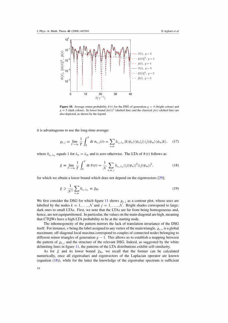
Interestingly, for the DSG, the overall shape of π(t) does not depend significantly on thesize of the gasket (figure 10). In fact, the behaviour of π(t) is mainly controlled by the mosthighly degenerate eigenvalues. These do not change when increasing the fractal size (i.e. itsgeneration). These values are 3 with degeneracy mg(3) = (3g−1 + 3)/2, 5 with degeneracymg(5) = (3g−1 − 1)/2 and (5 ± √

13)/2 with degeneracy mg−1(3), see section 3.

4.4. Long-time averages

As underlined in section 2, the unitary time evolution does not allow a definite long-time limitfor πk,j (t). Then, in order to obtain information about the overall spreading of quantum walks,

13

J. Phys. A: Math. Theor. 41 (2008) 445301 E Agliari et al

0 10 20 30 40

10

10

10

10

100

t(γ−1)

π(t

),|α

(t)|

2,p(t

)

π(t), g = 4

|α(t)|2, g = 4

p(t), g = 4

π(t), g = 5

|α(t)|2, g = 5

p(t), g = 5

Figure 10. Average return probability π(t) for the DSG of generation g = 4 (bright colour) andg = 5 (dark colour). Its lower bound |α(t)|2 (dashed line) and the classical p(t) (dotted line) arealso depicted, as shown by the legend.

it is advantageous to use the long-time average:

χk,j ≡ limT →∞

1

T

∫ T

0dt πk,j (t) =

∑n,m

δλn,λm〈k|ψn〉〈ψn|j 〉〈j |ψm〉〈ψm|k〉, (17)

where δλn,λmequals 1 for λn = λm and is zero otherwise. The LTA of π(t) follows as

χ ≡ limT →∞

1

T

∫ T

0dt π(t) = 1

N∑n,m,j

δλn,λm|〈j |ψn〉|2|〈j |ψm〉|2, (18)

for which we obtain a lower bound which does not depend on the eigenvectors [29]:

χ � 1

N 2

∑n,m

δλn,λm≡ χlb. (19)

We first consider the DSG for which figure 11 shows χk,j as a contour plot, whose axes arelabelled by the nodes k = 1, . . . ,N and j = 1, . . . ,N . Bright shades correspond to large;dark ones to small LTAs. First, we note that the LTAs are far from being homogeneous and,hence, are not equipartitioned. In particular, the values on the main diagonal are high, meaningthat CTQWs have a high LTA probability to be at the starting node.

The inhomogeneity of the pattern mirrors the lack of translation invariance of the DSGitself. For instance, v being the label assigned to any vertex of the main triangle, χv,v is a globalmaximum; off-diagonal local maxima correspond to couples of connected nodes belonging todifferent minor triangles of generation g − 1. This allows us to establish a mapping betweenthe pattern of χk,j and the structure of the relevant DSG. Indeed, as suggested by the whitedelimiting lines in figure 11, the patterns of the LTA distributions exhibit self-similarity.

As for χ and its lower bound χlb, we recall that the former can be calculatednumerically, once all eigenvalues and eigenvectors of the Laplacian operator are known(equation (18)), while for the latter the knowledge of the eigenvalue spectrum is sufficient

14

J. Phys. A: Math. Theor. 41 (2008) 445301 E Agliari et al

5 10 15 20 25

5

10

15

20

25

j

k

0.05

0.1

0.15

0.2

0.25

χk,j

20 40 60 80

10

20

30

40

50

60

70

80

j

k

0.05

0.1

0.15

0.2

χk,j

Figure 11. Limiting probabilities for the DSG of generation g = 3 (top) and g = 4 (bottom),whose volumes are N = 27 and N = 81, respectively. The white delimiting lines enclose thelimiting distributions for gaskets of smaller generations. Note that the global maxima lay on themain diagonal and correspond to j = 1, 14, 27 and to j = 1, 41, 81 for g = 3 and for g = 4,respectively.

(equation (19)). Since the spectrum of the DSG is known, we can calculate χlb analytically.Recalling the results of section 3, at generation g the spectrum of L displays N distincteigenvalues, where

N =g−1∑r=0

2r +g−2∑r=0

2r + 1 = 3 × 2g−1 − 1.

We call the set of distinct eigenvalues {λi}i=1,...,N . Being m(λi) the degeneracy of theeigenvalue λi , we can write

N 2χlb =N∑

n,m=1

δλn,λm=

N∑n=1

m(λn) =N∑

i=1

[m(λi)]2.

15

J. Phys. A: Math. Theor. 41 (2008) 445301 E Agliari et al

101

102

10

10

100

χ,χlb

0 100 200 300 4001

1.2

1.4

1.6

1.8

2

N

η

DSG, χ

DSG, χlb

CT, χ

CT, χlb

ST, χ

ST, χlb

equipartition 1/N

CT

ST

DSG

Figure 12. Long-time average χ and its lower bound χlb calculated according to equation (20) forthe dual Sierpinski gasket (diamonds and stars), the Cayley tree (triangles and diagonal crosses)and the square torus (crosses and open circles) versus the size of the structure N ; lines are guidesfor the eye. The dashed line represents the equipartition value 1/N . Inset shows the ratio η asa function of N . Note that η(N ) ≡ 1 holds not only for the periodic square lattice, but for allhypercubic lattices.

Now, we go over to the space of distinct degeneracies, each corresponding to a number ρ ofdistinct eigenvalues and we get the final, explicit formula

χ � χlb = 1

N 2

2g∑r=0

[m(r)]2ρ(m(r))

= 1

N 2

{g−1∑r=0

[3g−r−1 + 3

2

]2

× 2r +g−2∑r=0

[3g−r−1 − 1

2

]2

× 2r + 1

}

= 1

32g

[3g

(1 +

3g

14

)+

10

72g − 3

2

]>

1

3g. (20)

Interestingly, in the limit g → ∞, the LTA χ is finite:

χ � limg→∞ χlb = 1

14

and χlb reaches this asymptotic value from above.In figure 12 we show, as functions of N , χ and its lower bound, calculated from

equations (18) and (20). For comparison, the same quantities obtained for CTs and STsare also depicted. In the latter case, due to the regularity and periodicity of the lattice [40],the lower bound actually coincides with the exact value. For all cases considered, χ is largerthan the equipartition value (given by the dashed line).

The inset of figure 12 shows the ratio

η(N ) ≡ χ

χlb.

Obviously, the closer η is to 1, the better χlb approximates χ . In this sense, the lower boundcalculated for CTs is not as good an approximation to χ as is for the DSG and for the ST. For

16

J. Phys. A: Math. Theor. 41 (2008) 445301 E Agliari et al

the CT, χlb definitely underestimates, being about half the exact value of χ . The quantity η(N )

may act as a measure of the inhomogeneity of a given substrate. Practically, when dealingwith a large sized, sufficiently regular structure, we can get information about the localizationof a quantum particle moving on it simply through χlb, thus avoiding the (lengthy) evaluationof the eigenvector set.

5. Conclusions

We investigated the behaviour of continuous-time quantum walks on finite discrete structurescharacterized by different topologies; we considered the square torus, the Cayley tree and thedual Sierpinski gasket.

The interplay between the quantum-walk dynamics and the underlying topology wasdeepened by studying, in particular, the temporal evolution of the transfer probabilitydistribution and the ratio χ/χlb as a function of the substrate size. The latter turns out tobe significantly sensitive to the inhomogeneity of the substrate, from which we can infer thatlower-bound estimates are especially reliable for regular structures.

From an applied, as well as theoretical, perspective, the average displacement of thewalker, as a function of time, also plays an important role. This quantity is not only directlyrelated to the transport properties, but it also provides information about how fast the walkexplores the underlying structure, allowing an immediate comparison with the classical case.We found that at short times, CTQWs can spread faster than their classical counterparts,although spatial inhomogeneities and finiteness jointly reduce this effect. In the appendixwe prove that for infinite d-dimensional hypercubic lattices, at long times both the averagechemical and the Euclidean displacements depend linearly on time (i.e. the motion is ballistic);for finite lattices this kind of behaviour holds at relatively short times only.

Acknowledgments

EA thanks the Italian Foundation ‘Angelo della Riccia’ for financial support. Support fromthe Deutsche Forschungsgemeinschaft (DFG), the Fonds der Chemischen Industrie and theMinistry of Science, Research and the Arts of Baden-Wurttemberg (AZ: 24-7532.23-11-11/1)is gratefully acknowledged.

Appendix A. Average chemical displacement on hypercubic lattices

Here we consider infinite d-dimensional hypercubic lattices and, by exploiting theirtranslational invariance, we prove that on them the average chemical displacements of CTQWs,as defined in section 2.1, depend linearly on time. We first focus on the infinite discrete chain,then we consider the generic d-dimensional case and finally we analyse the two-dimensionallattice.

For a ring of length N , by exploiting the Bloch states, we have [41]

αk,j (t) = 1√N

∑l

e−iλl t e−il(k−j), (A.1)

where λl is the lth eigenvalue of the Laplacian matrix L associated with the ring. In the limitN → ∞ we are allowed to replace the sum over l by an integral, obtaining

limN→∞

αk,j (t) = ik−j e−i2t Jk−j (2t), (A.2)

17

J. Phys. A: Math. Theor. 41 (2008) 445301 E Agliari et al

where Jk(z) is the Bessel function of the first kind. In the calculation of the transfer probabilityπk,j (t) the phase factor vanishes and we have πk,j (t) = J 2

k−j (2t), which can be restated as

πk,0(t) = J 2k (2t), (A.3)

due to the translational invariance of the structure. Clearly (in agreement with πk,0(t) being aprobability distribution), one has for all t

+∞∑k=−∞

πk,0(t) =+∞∑

k=−∞J 2

k (2t) = J 20 (2t) + 2

∞∑k=1

J 2k (2t) = 1, (A.4)

the last equality being based on Jk(z) = (−1)kJ−k(z) and on equation (8.536.3) in [42].Now, the average chemical displacement of a CTQW which starts from 0 and moves on

an infinite chain (subscript q, 1) follows from equation (5) as

〈r0(t)〉q,1 = 〈r(t)〉q,1 =∑k∈V

(k, 0)J 2k (2t)

=∞∑

k=−∞|k|J 2

k (2t) = 2∞∑

k=1

kJ 2k (2t). (A.5)

Here, in the first equality we dropped the subscript 0 due to the equivalence between the sitesand in the last equality we exploited the symmetry of the Bessel functions, J 2

−k(z) = J 2k (z).

Now, recalling the recursion formula equation (8.471.1) in [42]

Jk−1(z) + Jk+1(z) = 2k

zJk(z), (A.6)

we can write

2∞∑

k=1

kJ 2k (z) = z

∞∑k=1

[Jk−1(z)Jk(z) + Jk(z)Jk+1(z)] ≡ zJ (z), (A.7)

by defining the function J (z). Hence⟨rk

(z

2

)⟩q,1

= zJ (z), (A.8)

where we put 2t = z. The squared Bessel function J 2k (z) is almost everywhere positive and

the analysis of its zeros allows us to state that, for t > 0, the sum appearing in the left-handside of equation (A.8) is strictly positive; the same holds therefore for J (z), for which we alsonote from equation (A.7) that J (0) = 0. Moreover, through the following recursion formula,equation (8.471.2) in [42]

2∂

∂zJk(z) = Jk−1(z) − Jk+1(z), (A.9)

it follows by directly differentiating J (z) and rearranging the terms

d

dzJ (z) = J0(z)[J0(z) + J2(z)]

2= J0(z)J1(z)

z, (A.10)

where in the last expression we again used equation (A.6) for k = 1. The indefinite integralof equation (A.10) is (see equation (5.53) in [42])

J (z) = zJ 20 (z) + zJ 2

1 (z) − J0(z)J1(z) + C, (A.11)

as can be simply verified by differentiating equation (A.11) and using equations (A.6) and(A.9). Furthermore, since J (0) = 0, we have C = 0.

18

J. Phys. A: Math. Theor. 41 (2008) 445301 E Agliari et al

Therefore, the following, for us fundamental, relation holds:∞∑

k=1

kJ 2k (z) = z

2

[zJ 2

0 (z) + zJ 21 (z) − J0(z)J1(z)

]. (A.12)

Now, from equations (A.5) and (A.12) we get the exact expression for the average chemicaldisplacement ⟨

r

(z

2

)⟩q,1

= z[zJ0(z)2 + zJ1(z)

2 − J0(z)J1(z)]. (A.13)

For large z = 2t (i.e. long times) we can use the expansion (see equation (8.451.1) in [42])

Jk(z) =√

2

πz

[cos

(z − kπ

2− π

4

)+ O

(1

z

)]. (A.14)

Consequently, inserting equation (A.14) for J0(z) and J1(z) into (A.13), we infer that thelong-time behaviour of the average chemical CTQW displacement on an infinite chain obeys

〈r(t)〉q,1 ∼ 4t

π. (A.15)

This result is consistent with findings reported in [39] for the average square displacement.Let us now consider higher-dimensional hypercubic lattices. Again, without loss of

generality, we can assume the CTQW to start from the point 0 = (0, 0, . . . , 0) so that thechemical distance attained by a walker being at the generic site k = (k1, k2, . . . , kd) is(k, 0) = |k1| + |k2| + · · · + |kd |. Furthermore, on a hypercubic lattice, assuming symmetricconditions in all directions, the probability distribution πk,0(t) factorizes into the d-independentone-dimensional distributions πkj ,0(t):

πk,0(t) = πk1,0(t)πk2,0(t) · · · πkd,0(t) =d∏

j=1

πkj ,0(t). (A.16)

Hence

〈r0(t)〉q,d =⟨

d∑j=1

|kj |⟩

q,d

=d∑

j=1

〈|kj |〉q,d =d∑

j=1

〈|kj |〉q,1 = d〈r0(t)〉q,1. (A.17)

In the last relation we used the fact that 〈|kj |〉q,d = 〈|kj |〉q,1 since for each j only thedistribution πkj ,0(t) matters, the other distributions adding up to a factor of unity each. Hence

〈r(t)〉q,d = d〈r(t)〉q,1 ∼ 4 dt

π. (A.18)

In particular, for the square lattice we have

〈r(t)〉q,2 ∼ 8t

π, (A.19)

which was used in figure A1 (dashed line) to fit data relevant to the average chemicaldisplacement performed by a CTQW on square tori of different (finite) sizes. As can beseen from the figure, the ballistic behaviour also holds for finite lattices, but for relatively shorttimes only: at longer times the finiteness of the lattice starts to matter and the product of Besselfunctions in equation (A.16) ceases to be a good approximation of the transfer probability.When the waves associated with CTQWs have crossed the whole lattice, interference effectsstart to occur and 〈r(t)〉q,2 exhibits a non-monotonic behaviour. From the same figure we alsonote that the O(1/t) contributions of equation (A.14) get to be negligible for t > 1γ −1.

19

J. Phys. A: Math. Theor. 41 (2008) 445301 E Agliari et al

Figure A1. Average chemical displacement 〈r(t)〉q for the torus, calculated according toequation (6) (symbols); the line represents the Euclidean average displacement for L = 19.The dotted and the dashed lines highlight the linear dependence on t exhibited by the averagechemical distance and by the average Euclidean distance, respectively.

In figure A1 we also show data for the average Euclidean displacement which displaysa ballistic behaviour at short times as well. Indeed, for a hypercubic lattice of arbitrarydimension d, the following relation holds (see e.g. [43]):

1√3(k, j) � ‖k − j‖ � (k, j), (A.20)

where ‖k − j‖ denotes the Euclidean distance between the lattice points k and j chosenarbitrarily. By averaging each term of the previous equation with respect to the transferprobability πk,j(t) (we can again exploit the translational invariance of the substrate and fixj = 0), we find that the average Euclidean distance also scales linearly with time with amultiplicative factor bounded between 4d/(

√3π) ≈ 2.31d/π and 4d/π . In particular, for

the square torus of size L = 19 considered in figure A1, we find that at relatively short timesthe average Euclidean distance scales as 6t/π .

References

[1] Kempe J 2003 Contemp. Phys. 44 307[2] Sanders B C, Bartlett S D, Tregenna B and Knight P L 2003 Phys. Rev. A 67 042305[3] Lahini Y, Avidan A, Pozzi F, Sorel M, Morandotti R, Christodoulides D N and Silberberg Y 2008 Phys. Rev. Lett.

100 013906[4] Dur W, Raussendorf R, Kendon V M and Briegel H-J 2002 Phys. Rev. A 66 052319[5] Cote R, Russell A, Eyler E E and Gould P L 2006 New J. Phys. 8 156[6] Zou X, Dong Y and Guo G 2006 New J. Phys. 8 81[7] Ryan C A, Laforest M, Boileau J C and Laflamme R 2005 Phys. Rev. A 72 062317[8] Mulken O, Blumen A, Amthor T, Giese C, Reetz-Lamour M and Weidemuller M 2007 Phys. Rev. Lett.

99 090601[9] Aharonov Y, Davidovich L and Zagury N 1993 Phys. Rev. A 48 1687

[10] Farhi E and Gutmann S 1998 Phys. Rev. A 58 915

20

J. Phys. A: Math. Theor. 41 (2008) 445301 E Agliari et al

[11] Strauch F W 2006 Phys. Rev. A 74 030301[12] Štefanak M, Jex I and Kiss T 2008 Phys. Rev. Lett. 100 020501[13] Volta A, Mulken O and Blumen A 2006 J. Phys. A: Math. Gen. 39 14997[14] Mulken O, Pernice V and Blumen A 2007 Phys. Rev. E 76 051125[15] ben-Avraham D and Havlin S 2001 Diffusion and Reactions in Fractals and Disordered Systems (Cambridge:

Cambridge University Press)[16] Vidal J, Mosseri R and Bellissard J 1999 J. Phys. A: Math. Gen. 32 2361[17] Williams C P 2001 Comput. Sci. Eng. 3 44[18] Ambainis A 2004 SIGACT News 35 22[19] Magniez F, Nayak A, Roland J and Santha M 2007 Proc. ACM Symp. on Theory of Computation (STOC’07)

(New York: ACM) p 575[20] Yin Y, Katsanos D E and Evangelou S N 2008 Phys. Rev. A 77 022302[21] Yuan H Q, Grimm U, Repetowicz P and Schreiber M 2000 Phys. Rev. B 62 15569[22] Alavi Y, Chartrand G, Oellermann O R and Schwenk A J (ed) Graph Theory, Combinatorics, and Applications

vol 2 (NewYork: Wiley)[23] Di Vincenzo D P 1995 Science 270 255[24] Childs A M and Goldstone J 2004 Phys. Rev. A 70 022314[25] Mulken O, Volta A and Blumen A 2005 Phys. Rev. A 72 042334[26] Weiss G H 1994 Aspects and Applications of the Random Walk (Amsterdam: North-Holland)[27] Aharonov D, Ambainis A, Kempe J and Vazirani U 2001 Proc. ACM Symp. on Theory of Computation (STOC’01)

(New York: ACM) p 50[28] Aarao Reis F D A 1995 J. Phys. A: Math. Gen. 28 6277[29] Mulken O 2007 arXiv:0710.3453[30] Mulken O and Blumen A 2006 Phys. Rev. E 73 066117[31] Mulken O, Bierbaum V and Blumen A 2006 J. Chem. Phys. 124 124905[32] Konno N 2006 Quantum Probab. Relat. Top. 9 287[33] Konno N 2006 Int. J. Quantum Inf. 4 1023[34] Cosenza M G and Kapral R 1992 Phys. Rev. A 46 1850[35] Blumen A and Jurjiu A 2002 J. Chem. Phys. 116 2636[36] Cerovski V Z, Schreiber M and Grimm U 2005 Phys. Rev. B 72 054203[37] Anderson PW 1958 Phys. Rev. 109 1492[38] Monastyrsky M I 2006 Topology in Condensed Matter (Springer Series in Solid-State Sciences) (Berlin:

Springer)[39] Katsanos D E, Evangelou S N and Xiong S J 1995 Phys. Rev. B 51 895[40] Blumen A, Bierbaum V and Mulken O 2006 Physica A 371 10[41] Mulken O and Blumen A 2005 Phys. Rev. E 71 036128[42] Gradshteyn I S and Ryzhik I M 1965 Table of Integrals, Series and Products (NewYork: Academic)[43] Searcoid M O 2007 Metric Spaces (London: Springer)

21