1

Dynamics of cell wall elasticity pattern shapes the cell during yeast mating

morphogenesis.

Björn Goldenbogen1, Wolfgang Giese1, Marie Hemmen1, Jannis Uhlendorf1,

Andreas Herrmann2, Edda Klipp1

1. Institute of Biology, Theoretical Biophysics, Humboldt-Universität zu Berlin,

Invalidenstraße 42, 10115 Berlin

2. Institute of Biology, Molecular Biophysics, Humboldt-Universität zu Berlin,

Invalidenstraße 42, 10115 Berlin

Content

Supporting Text S1 ............................................................................................................................................................. 1 Dynamic Cell Wall Models (DM) .................................................................................................... 1

Steady State Cell Wall Model (SM) .............................................................................................. 6

References ............................................................................................................................................... 9

Figures S1 - S13 ................................................................................................................................................................10 Table S1 Parameters values used in the models ..........................................................................................24

Supporting Text S1

Dynamic Cell Wall Models (DM)

We developed a computational model to simulate inhomogeneous elasticity and

elasto-plastic growth due to internal turgor pressure in space and time. The approach

is based on continuum mechanics, where plane stress for thin shells is assumed.

The cell wall is discretized into a triangular mesh using the finite element mesh

generator Gmsh (Geuzaine and Remacle 2009) and simulations are performed with

the general purpose finite element framework DUNE (Bastian et al. 2008). We

simulated the model equations in different situations for a wide range of parameters.

Furthermore, the analytical results derived for the steady state model (SM) were

compared and matched with the dynamic models DM1 and DM2.

2

First, we introduce the elastic properties of a single triangle in the discretization of the

cell wall as suggested by Delingette (Delingette 2008). Let T be a triangle of the cell

wall discretization, where the points of the undeformed triangle are denoted by ,

and the points of the elastically deformed triangle are denoted by , , , as

depicted in figure S10. In the remainder, we refer to the elastically undeformed and

deformed state of the triangle also as relaxed and stretched triangle, respectively.

The area of the relaxed and stretched triangle is denoted as and , respectively.

The evolution of the cell wall was described by a deformation function . The

right Cauchy-Green deformation tensor was computed from

(1)

and the Green-Lagrange strain tensor from

(2)

These tensors were used to calculate the elastic energy, elastic forces and yield

criteria. There are three important quantities that were expressed in terms of angles

and length of the sides of the deformed and the relaxed triangle (Delingette 2008):

(

) (3)

(

) (4)

. (5)

Here, and are the lengths and and are areas of the relaxed triangle and

stretched triangle, respectively. The angles of the relaxed triangle are denoted by

. A sketch of the relaxed state and stretched triangle can be found in figure S10.

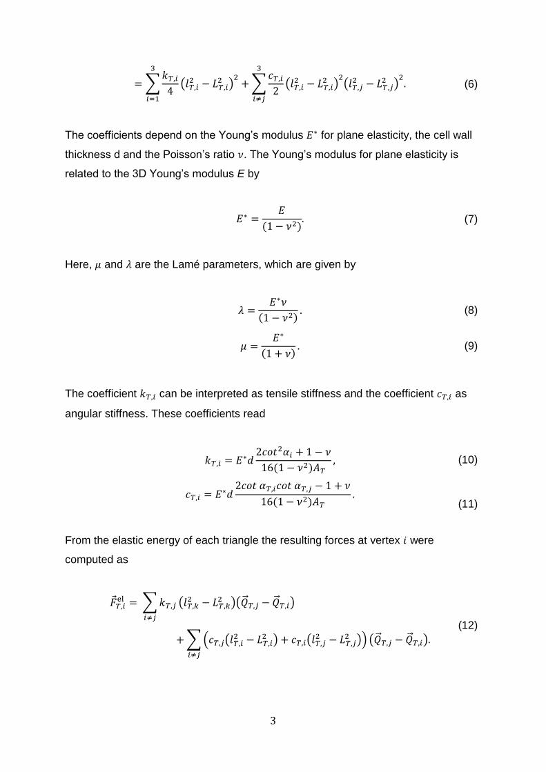
The elastic energy of a single triangle T with thickness d is given by

3

∑

(

) ∑

(

) (

)

(6)

The coefficients depend on the Young’s modulus for plane elasticity, the cell wall

thickness d and the Poisson’s ratio . The Young’s modulus for plane elasticity is

related to the 3D Young’s modulus E by

(7)

Here, and are the Lamé parameters, which are given by

(8)

(9)

The coefficient can be interpreted as tensile stiffness and the coefficient as

angular stiffness. These coefficients read

(10)

(11)

From the elastic energy of each triangle the resulting forces at vertex were

computed as

∑

(

)( )

∑( (

) (

))

( )

(12)

4

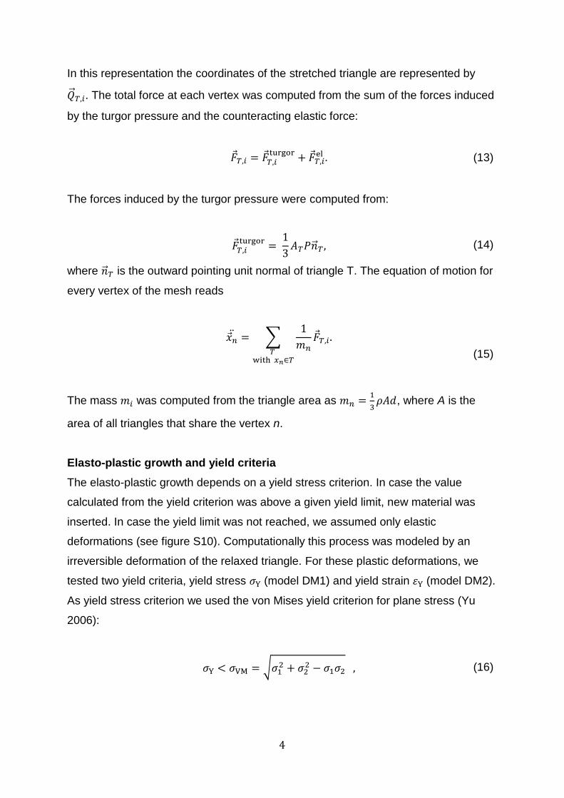
In this representation the coordinates of the stretched triangle are represented by

. The total force at each vertex was computed from the sum of the forces induced

by the turgor pressure and the counteracting elastic force:

(13)

The forces induced by the turgor pressure were computed from:

(14)

where is the outward pointing unit normal of triangle T. The equation of motion for

every vertex of the mesh reads

∑

(15)

The mass was computed from the triangle area as

, where A is the

area of all triangles that share the vertex n.

Elasto-plastic growth and yield criteria

The elasto-plastic growth depends on a yield stress criterion. In case the value

calculated from the yield criterion was above a given yield limit, new material was

inserted. In case the yield limit was not reached, we assumed only elastic

deformations (see figure S10). Computationally this process was modeled by an

irreversible deformation of the relaxed triangle. For these plastic deformations, we

tested two yield criteria, yield stress (model DM1) and yield strain (model DM2).

As yield stress criterion we used the von Mises yield criterion for plane stress (Yu

2006):

√

(16)

5

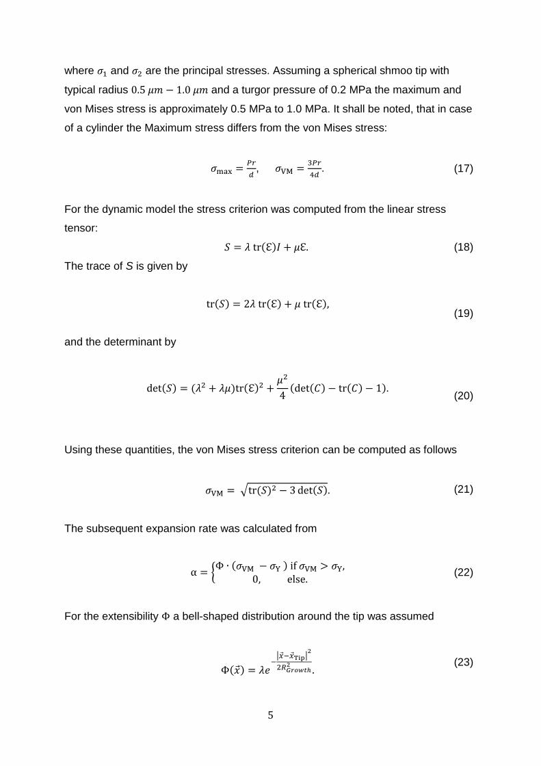
where and are the principal stresses. Assuming a spherical shmoo tip with

typical radius and a turgor pressure of 0.2 MPa the maximum and

von Mises stress is approximately 0.5 MPa to 1.0 MPa. It shall be noted, that in case

of a cylinder the Maximum stress differs from the von Mises stress:

,

. (17)

For the dynamic model the stress criterion was computed from the linear stress

tensor:

(18)

The trace of S is given by

(19)

and the determinant by

(20)

Using these quantities, the von Mises stress criterion can be computed as follows

√ (21)

The subsequent expansion rate was calculated from

{

(22)

For the extensibility a bell-shaped distribution around the tip was assumed

| |

(23)

6

The expansion of the cell wall was modeled as elongation of the edges of the relaxed

triangle. Let and be two adjacent triangles and the relaxed length of the

edge that both triangles share. The expansion rates and were calculated as

above for the triangles and , respectively. The elongation of the edge is

given by

(24)

For the DM2 we modelled cell wall expansion upon a yield strain. Here, we used the

volumetric strain as a measure for yielding:

(25)

The extensibility is in this case given by ⁄ . Which leads to the

expansion rate

{

(26)

The elongation of the edge is then analogously given by

(

) (27)

Steady State Cell Wall Model (SM)

In a mechanistic model for the cell shape, it is crucial to describe the distribution of

forces due to turgor pressure, material insertion and the counterbalancing forces,

which can be derived from the material properties of the cell wall. The first basic

relationship connects the stresses (force per unit area) on the cell wall to the turgor

pressure , the cell wall thickness and the local geometry. The latter is

characterized by the principal curvatures. We assumed the cell shape to have a

rotational symmetry and the shape of the cell was described as a surface of rotation.

7

The distribution of the corresponding stresses are expressed in terms of curvatures

(Flügge 1973):

,

(

). (28)

Here, the principal curvatures are given by the meridional curvature, , and the

circumferential curvature, . The stresses were connected to the strains with a

constitutive relationship for linear elasticity (Flügge 1973)

(

)

(

) (

), (29)

where is the Young’s modulus for plane elasticity, is the Poisson’s ratio,

and are the meridional and circumferential strain, respectively. The Young’s

modulus and strains are functions depending on the arc length .

Here,

and

are the meridional and circumferential strain,

respectively. While denotes a small relaxed and the actual extend of a small

surface patch in meridional direction, is the meridional distance of the relaxed

shape measured from the base end. Note, in all figures the arclength is plotted from

the tip instead of the base for better comparison to the dynamic model (see figure

S11). As for the dynamic model, the von Mises stress and volumetric strain are given

by:

√

(30)

(31)

From equations (28) and (29) we can derive a relationship between circumferential

and meridional strain, which only depends on the geometry and the Poisson’s ratio

(32)

Using this relationship, we get the formula

8

((

)

) , (33)

(see also (Bernal, Rojas, and Dumais 2007)), which was used to identify points of the

relaxed and natural shape of the cell starting from the end of the base. Therefore,

strains and stresses were calculated from the parameters and and the

geometry of the relaxed and natural shape only. Note, that the strains were not

calculated in the growth region, since we assumed plastic growth at the shmoo tip.

Inserting this relationship in the constitutive model we get:

(

(

)

). (34)

For a given cellular geometry, the elasticity distribution was computed from (Bernal,

Rojas, and Dumais 2007):

(

(

)

). (35)

We calculated the stress and elasticity distribution for the shmoo shape shown in

figure 1 (see main text) and figure S2. For the numerical computations, cubic spline

functions were used to characterize the shape. The NumPy and SciPy packages in

Python were used for this purpose. Calculations for different assumptions on relaxed

and extended cell shape and strains are shown in figure S2.

In the special case of a sphere or a cylinder, the strains, the stresses and the

elasticity can be computed analytically ( see figure S1). For a sphere, the

circumferential and meridional strain are given by

, (36)

and the principal stresses are given by

, (37)

9

Assuming a spherical geometry at the base as well as tip, the Young’s modulus the

tip can be approximated by the following formula:

(38)

This formula was used to compare the Young’s Modulus obtained from AFM

measurements and the Young’s modulus estimated by osmotic shock experiments.

References

Bastian, P, M Blatt, A Dedner, C Engwer, R Kloefkorn, R Kornhuber, M Ohlberger,

and O Sander. 2008. “A Generic Grid Interface for Parallel and Adaptive

Scientific Computing. Part II: Implementation and Tests in DUNE.” Computing 82

(2-3): 121–38. doi:10.1007/s00607-008-0004-9.

Bernal, Roberto, Enrique Rojas, and Jacques Dumais. 2007. “The Mechanics of Tip

Growth Morphogenesis: What We Have Learned From Rubber Balloons.” Journal

of Mechanics of Materials and Structures 2 (6): 1157–68.

doi:10.2140/jomms.2007.2.1157.

Delingette, Herve. 2008. “Triangular Springs for Modeling Nonlinear Membranes.”

Ieee Transactions on Visualization and Computer Graphics 14 (2): 329–41.

doi:10.1109/TVCG.2007.70431.

Flügge, Wilhelm. 1973. Stresses in Shells. Second. Springer-Verlag, New York-

Heidelberg. doi:10.1007/978-3-642-88291-3.

Geuzaine, Christophe, and Jean-Francois Remacle. 2009. “Gmsh: a 3-D Finite

Element Mesh Generator with Built-in Pre- and Post-Processing Facilities.”

International Journal for Numerical Methods in Engineering 79 (11): 1309–31.

doi:10.1002/nme.2579.

Yu, Mao-Hong. 2006. Generalized Plasticity. Springer Science & Business Media.

10

Figures S1 - S13

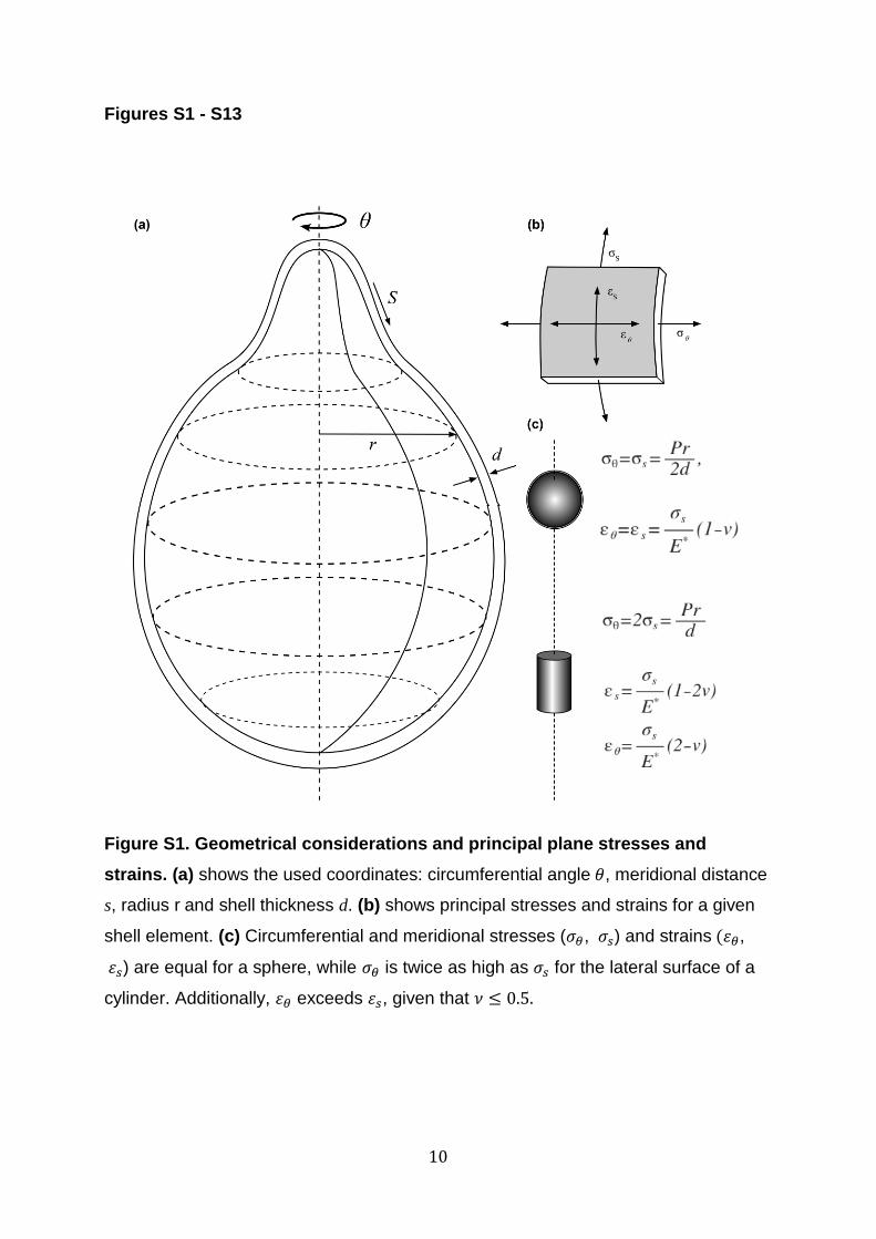
Figure S1. Geometrical considerations and principal plane stresses and

strains. (a) shows the used coordinates: circumferential angle , meridional distance

s, radius r and shell thickness d. (b) shows principal stresses and strains for a given

shell element. (c) Circumferential and meridional stresses ( , ) and strains ,

) are equal for a sphere, while is twice as high as for the lateral surface of a

cylinder. Additionally, exceeds , given that

11

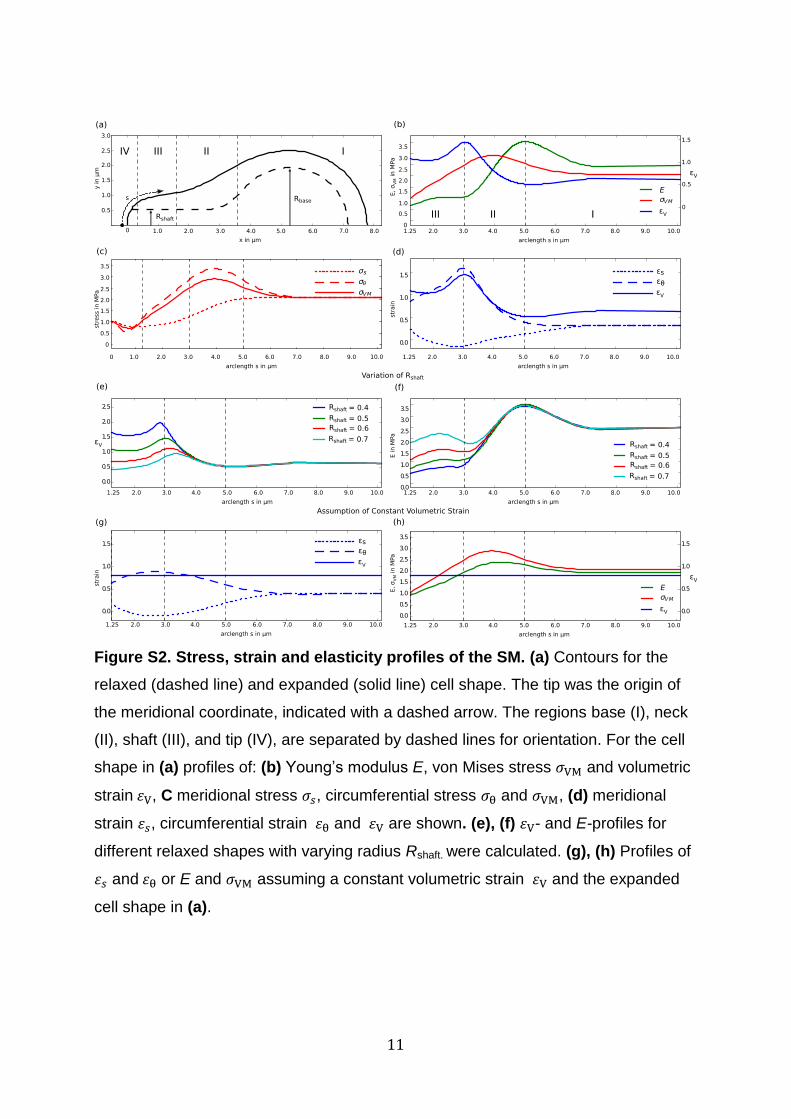
Figure S2. Stress, strain and elasticity profiles of the SM. (a) Contours for the

relaxed (dashed line) and expanded (solid line) cell shape. The tip was the origin of

the meridional coordinate, indicated with a dashed arrow. The regions base (I), neck

(II), shaft (III), and tip (IV), are separated by dashed lines for orientation. For the cell

shape in (a) profiles of: (b) Young’s modulus E, von Mises stress and volumetric

strain , C meridional stress , circumferential stress and , (d) meridional

strain , circumferential strain and are shown. (e), (f) - and E-profiles for

different relaxed shapes with varying radius Rshaft. were calculated. (g), (h) Profiles of

and or E and assuming a constant volumetric strain and the expanded

cell shape in (a).

12

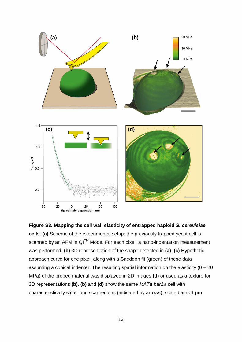
Figure S3. Mapping the cell wall elasticity of entrapped haploid S. cerevisiae

cells. (a) Scheme of the experimental setup: the previously trapped yeast cell is

scanned by an AFM in QITM Mode. For each pixel, a nano-indentation measurement

was performed. (b) 3D representation of the shape detected in (a). (c) Hypothetic

approach curve for one pixel, along with a Sneddon fit (green) of these data

assuming a conical indenter. The resulting spatial information on the elasticity (0 – 20

MPa) of the probed material was displayed in 2D images (d) or used as a texture for

3D representations (b). (b) and (d) show the same MATa bar1∆ cell with

characteristically stiffer bud scar regions (indicated by arrows); scale bar is 1 µm.

13

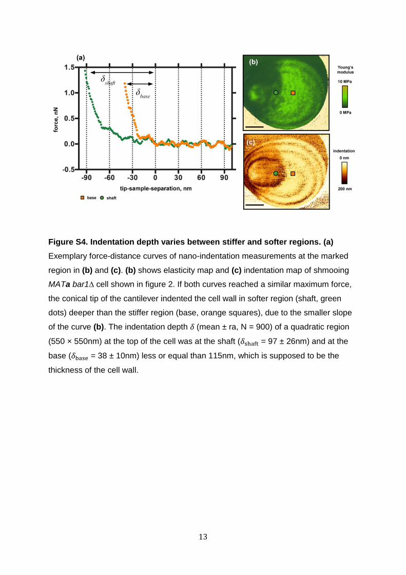
Figure S4. Indentation depth varies between stiffer and softer regions. (a)

Exemplary force-distance curves of nano-indentation measurements at the marked

region in (b) and (c). (b) shows elasticity map and (c) indentation map of shmooing

MATa bar1∆ cell shown in figure 2. If both curves reached a similar maximum force,

the conical tip of the cantilever indented the cell wall in softer region (shaft, green

dots) deeper than the stiffer region (base, orange squares), due to the smaller slope

of the curve (b). The indentation depth (mean ± ra, N = 900) of a quadratic region

(550 × 550nm) at the top of the cell was at the shaft ( = 97 ± 26nm) and at the

base ( = 38 ± 10nm) less or equal than 115nm, which is supposed to be the

thickness of the cell wall.

14

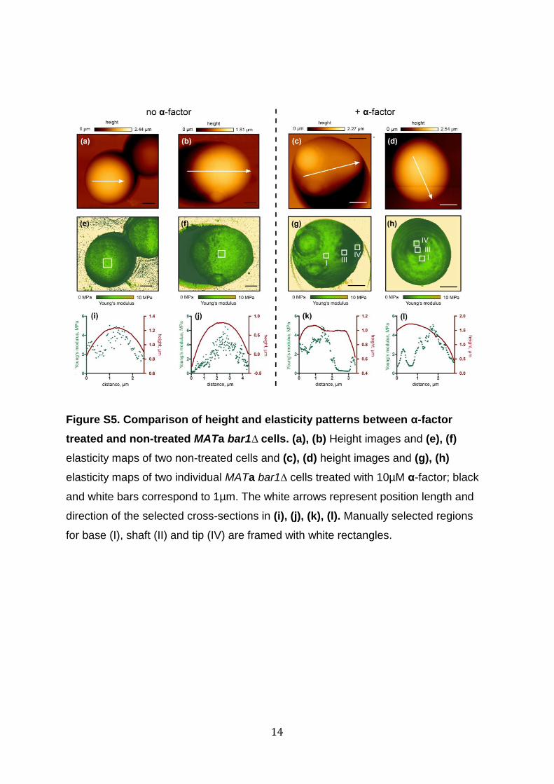
Figure S5. Comparison of height and elasticity patterns between α-factor

treated and non-treated MATa bar1∆ cells. (a), (b) Height images and (e), (f)

elasticity maps of two non-treated cells and (c), (d) height images and (g), (h)

elasticity maps of two individual MATa bar1∆ cells treated with 10µM α-factor; black

and white bars correspond to 1µm. The white arrows represent position length and

direction of the selected cross-sections in (i), (j), (k), (l). Manually selected regions

for base (I), shaft (II) and tip (IV) are framed with white rectangles.

15

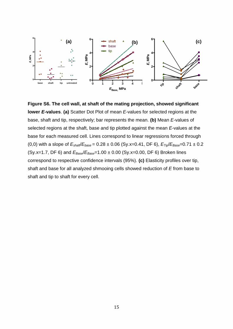
Figure S6. The cell wall, at shaft of the mating projection, showed significant

lower E-values. (a) Scatter Dot Plot of mean E-values for selected regions at the

base, shaft and tip, respectively; bar represents the mean. (b) Mean E-values of

selected regions at the shaft, base and tip plotted against the mean E-values at the

base for each measured cell. Lines correspond to linear regressions forced through

(0,0) with a slope of Eshaft/Ebase = 0.28 ± 0.06 (Sy.x=0.41, DF 6), ETip/EBase=0.71 ± 0.2

(Sy.x=1.7, DF 6) and EBase/EBase=1.00 ± 0.00 (Sy.x=0.00, DF 6) Broken lines

correspond to respective confidence intervals (95%). (c) Elasticity profiles over tip,

shaft and base for all analyzed shmooing cells showed reduction of E from base to

shaft and tip to shaft for every cell.

base shaft tip untreated

0

2

4

6

E, M

Pa

0 1 2 3 4 50

2

4

6

EBase, MPaE

, MP

a

shaft

base

tip

tip

shaf

t

base

0

2

4

6

E, M

Pa

(a) (c) (b)

16

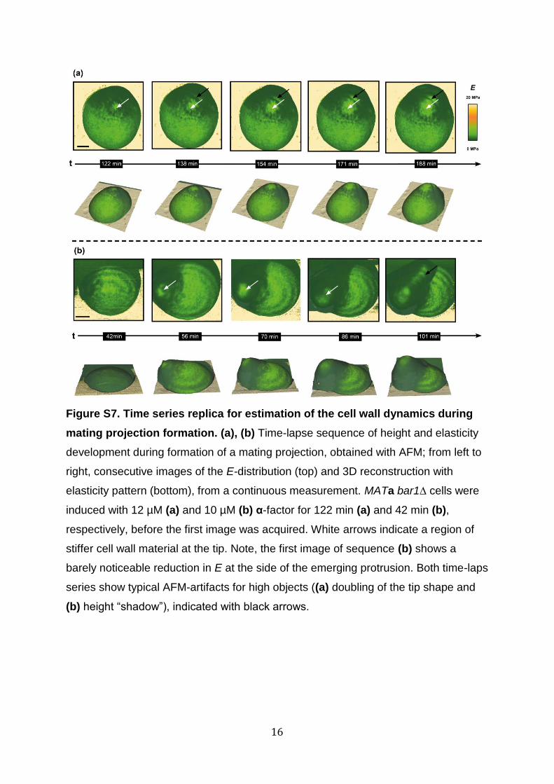
Figure S7. Time series replica for estimation of the cell wall dynamics during

mating projection formation. (a), (b) Time-lapse sequence of height and elasticity

development during formation of a mating projection, obtained with AFM; from left to

right, consecutive images of the E-distribution (top) and 3D reconstruction with

elasticity pattern (bottom), from a continuous measurement. MATa bar1∆ cells were

induced with 12 µM (a) and 10 µM (b) α-factor for 122 min (a) and 42 min (b),

respectively, before the first image was acquired. White arrows indicate a region of

stiffer cell wall material at the tip. Note, the first image of sequence (b) shows a

barely noticeable reduction in E at the side of the emerging protrusion. Both time-laps

series show typical AFM-artifacts for high objects ((a) doubling of the tip shape and

(b) height “shadow”), indicated with black arrows.

17

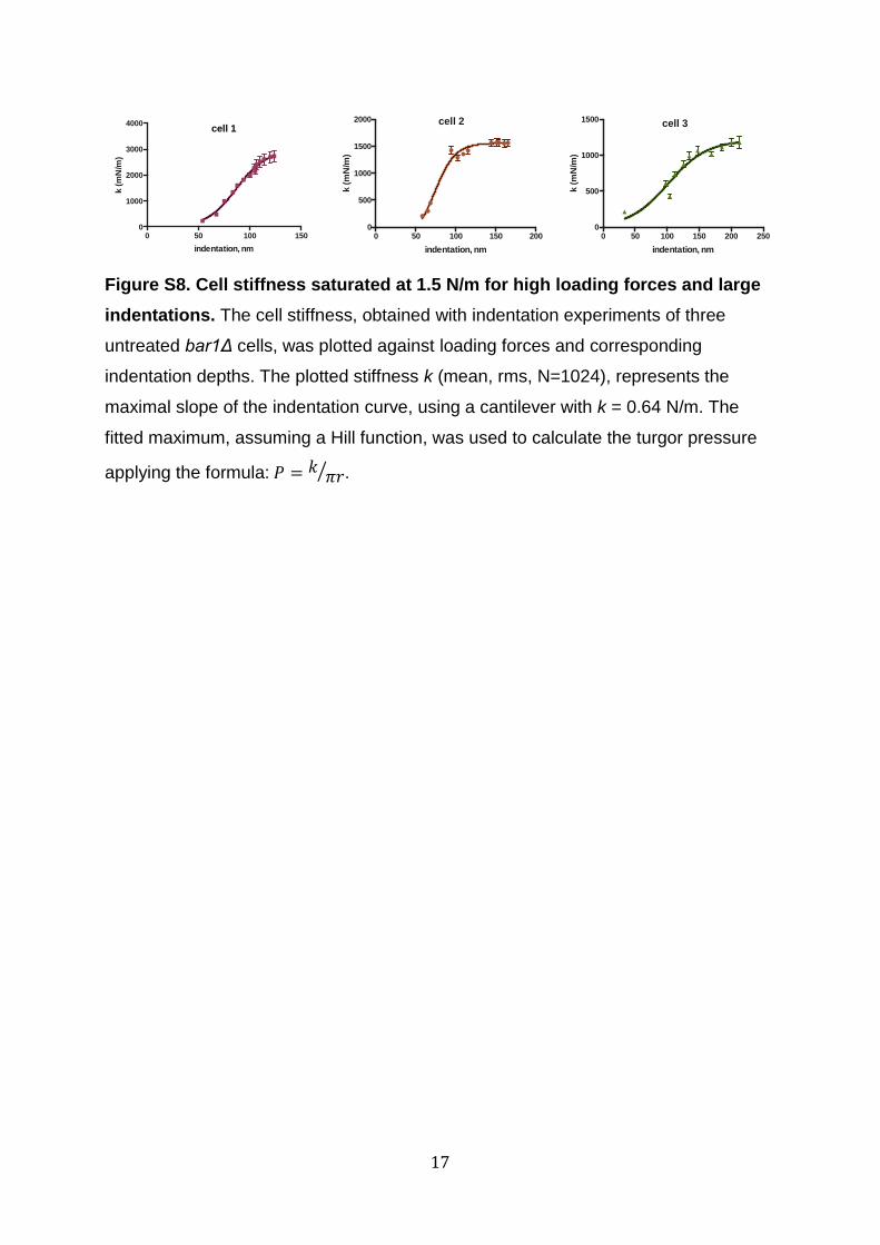
Figure S8. Cell stiffness saturated at 1.5 N/m for high loading forces and large

indentations. The cell stiffness, obtained with indentation experiments of three

untreated bar1Δ cells, was plotted against loading forces and corresponding

indentation depths. The plotted stiffness k (mean, rms, N=1024), represents the

maximal slope of the indentation curve, using a cantilever with k = 0.64 N/m. The

fitted maximum, assuming a Hill function, was used to calculate the turgor pressure

applying the formula: ⁄ .

0 50 100 1500

1000

2000

3000

4000

indentation, nm

k (

mN

/m)

cell 1

0 50 100 150 2000

500

1000

1500

2000

indentation, nm

k (m

N/m

)

cell 2

0 50 100 150 200 2500

500

1000

1500

indentation, nm

k (m

N/m

)

cell 3

18

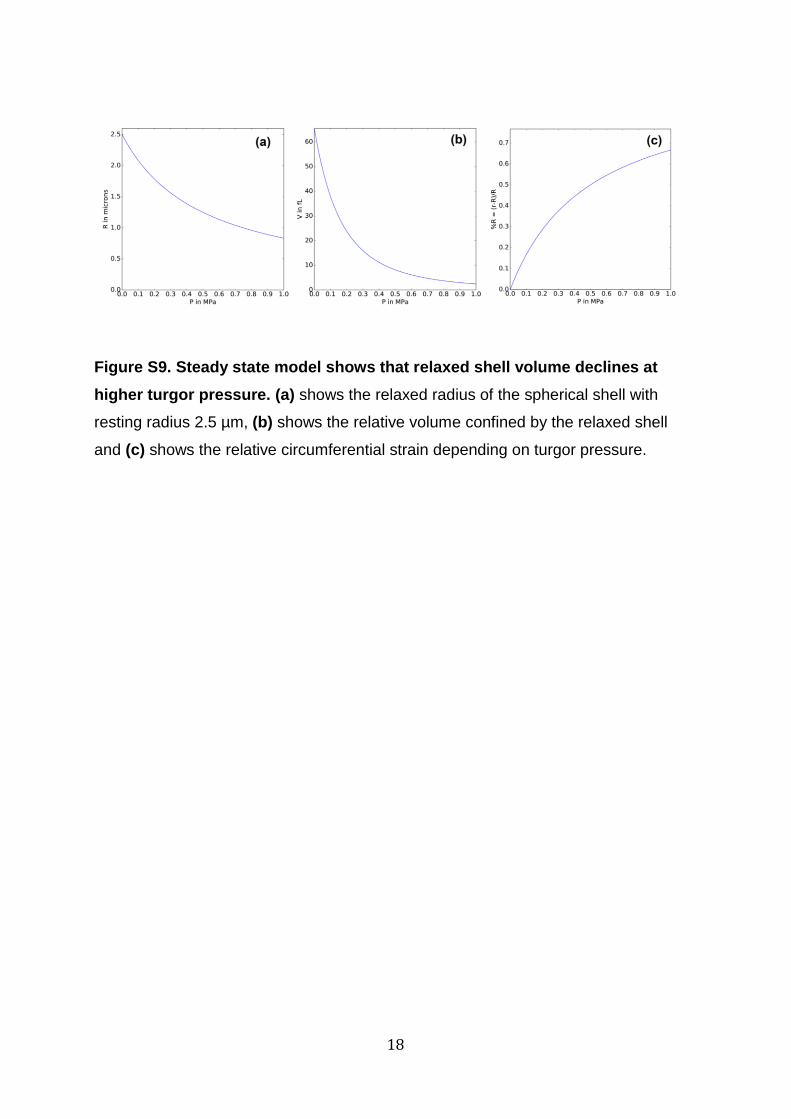
Figure S9. Steady state model shows that relaxed shell volume declines at

higher turgor pressure. (a) shows the relaxed radius of the spherical shell with

resting radius 2.5 µm, (b) shows the relative volume confined by the relaxed shell

and (c) shows the relative circumferential strain depending on turgor pressure.

19

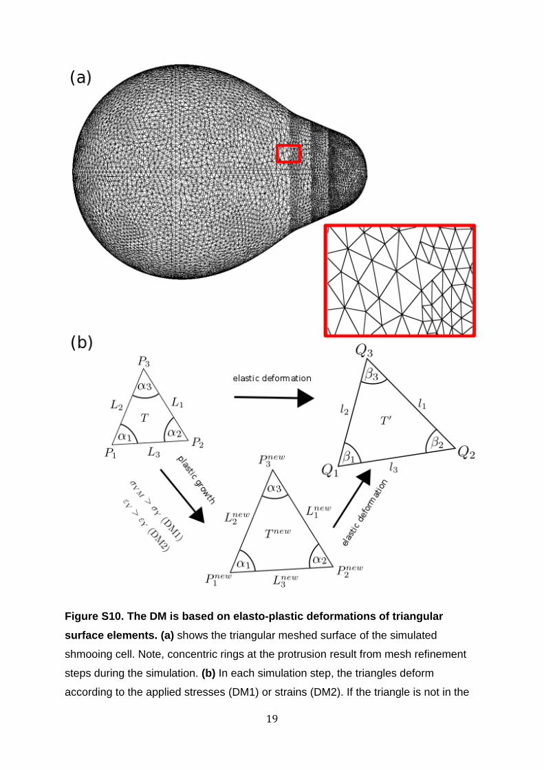
Figure S10. The DM is based on elasto-plastic deformations of triangular

surface elements. (a) shows the triangular meshed surface of the simulated

shmooing cell. Note, concentric rings at the protrusion result from mesh refinement

steps during the simulation. (b) In each simulation step, the triangles deform

according to the applied stresses (DM1) or strains (DM2). If the triangle is not in the

20

defined growth zone, the triangle deforms purely elastically. , , are the

relaxed lengths of the unstressed triangle and and , , are the elastically

expanded lengths of the resulting triangle . Correspondingly, , , represent

relaxed angles and , , angles of the deformed triangle. Additionally, triangles

in the defined growth zone deform plastically if > (DM1) or > (DM2).

Thereby, relaxed lengths expand to new relaxed lengths, ,

and , while

angles remain unaltered.

21

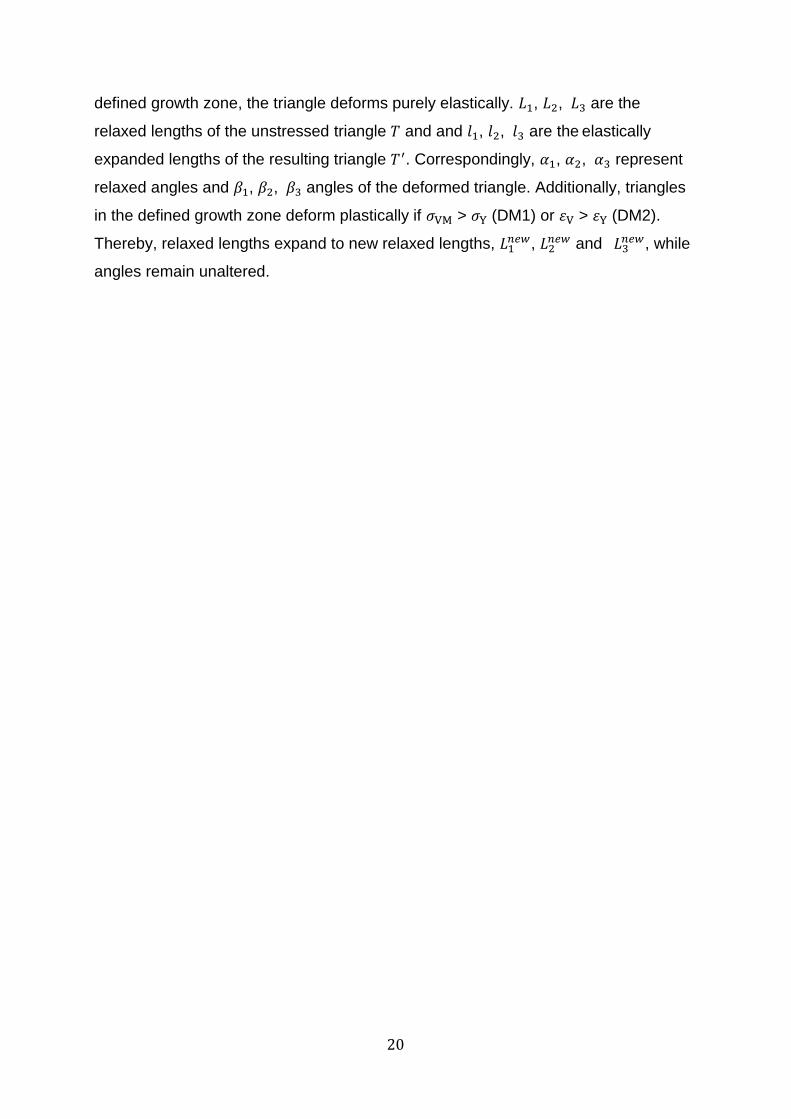
Figure S11. Simulated stress, strain and elasticity profiles along the cell

contour. (a) Contours of the resulting cell shape of DM1 (yellow) and DM2 (blue) at

time 3250 s with indicated regions: base (I), shaft (II), neck (III) and tip (IV). (b), (c),

(d) Contour plots along the arc length of the resulting von Mises stress , the

resulting volumetric strain and the assumed Young’s modulus .

22

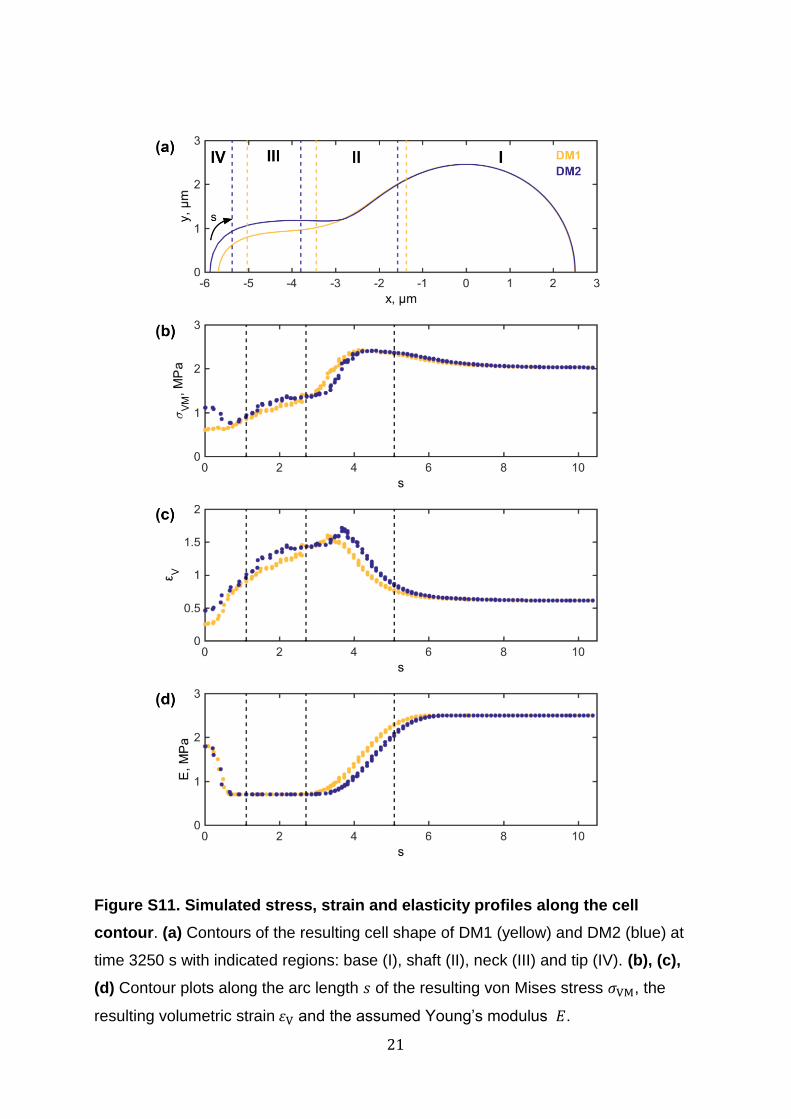
Figure S12. Sensitivity analysis of the yield limit for DM1 and DM2. (a) and (b)

show cell shapes obtained from simulations with various limits for yield stress and

yield strain , respectively at 1000 s, 1500 s and 2000 s. Lower or lower result

in faster growth. When varying parameters in a certain range, similar shapes are

obtained at different time points.

23

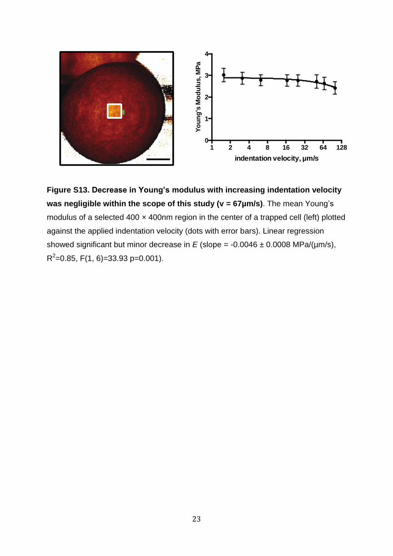
Figure S13. Decrease in Young’s modulus with increasing indentation velocity

was negligible within the scope of this study (v = 67µm/s). The mean Young’s

modulus of a selected 400 × 400nm region in the center of a trapped cell (left) plotted

against the applied indentation velocity (dots with error bars). Linear regression

showed significant but minor decrease in E (slope = -0.0046 ± 0.0008 MPa/(µm/s),

R2=0.85, F(1, 6)=33.93 p=0.001).

1 2 4 8 16 32 64 1280

1

2

3

4

indentation velocity, µm/s

Yo

un

g's

Mo

du

lus, M

Pa

24

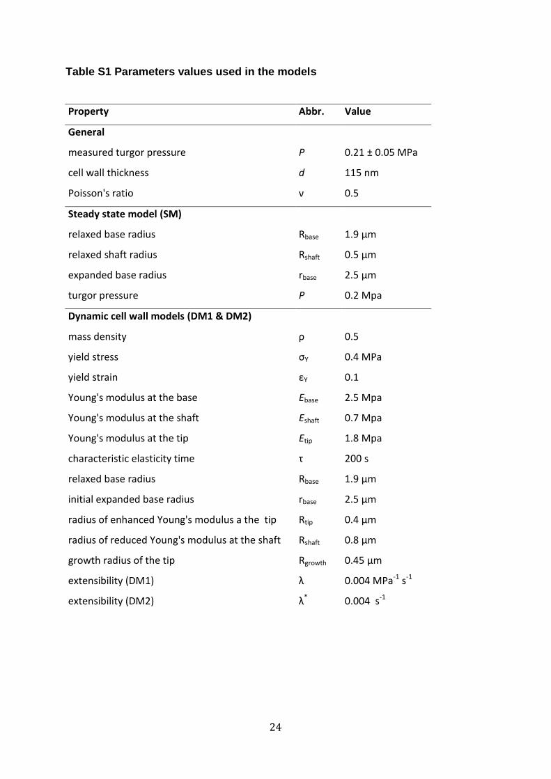
Table S1 Parameters values used in the models

Property Abbr. Value

General

measured turgor pressure P 0.21 ± 0.05 MPa

cell wall thickness d 115 nm

Poisson's ratio ν 0.5

Steady state model (SM)

relaxed base radius Rbase 1.9 µm

relaxed shaft radius Rshaft 0.5 µm

expanded base radius rbase 2.5 µm

turgor pressure P 0.2 Mpa

Dynamic cell wall models (DM1 & DM2)

mass density ρ 0.5

yield stress σY 0.4 MPa

yield strain εY 0.1

Young's modulus at the base Ebase 2.5 Mpa

Young's modulus at the shaft Eshaft 0.7 Mpa

Young's modulus at the tip Etip 1.8 Mpa

characteristic elasticity time τ 200 s

relaxed base radius Rbase 1.9 µm

initial expanded base radius rbase 2.5 µm

radius of enhanced Young's modulus a the tip Rtip 0.4 µm

radius of reduced Young's modulus at the shaft Rshaft 0.8 µm

growth radius of the tip Rgrowth 0.45 µm

extensibility (DM1) λ 0.004 MPa-1 s-1

extensibility (DM2) λ* 0.004 s-1