DYNAMICS IN THE HILL PROBLEM WITH …...DYNAMICS IN THE HILL PROBLEM WITH APPLICATIONS TO SPACECRAFT MANEUVERS by Benjamin F. Villac A dissertation submitted in partial fulﬁllment

DYNAMICS IN THE HILL PROBLEMWITH APPLICATIONS TO SPACECRAFT MANEUVERS

by

Benjamin F. Villac

A dissertation submitted in partial fulfillment

of the requirements for the degree of

Doctor of Philosophy

(Aerospace Engineering)

in The University of Michigan

2003

Doctoral committee:

Associate Professor Daniel J. Scheeres, ChairmanProfessor Anthony M. BlochProfessor Pierre T. KabambaProfessor Harris N. McClamrochProfessor Ralf J. Spatzier

c Benjamin F. Villac

All Rights Reserved2003

To my mother, Marie-Chantal

ii

ACKNOWLEDGEMENTS

I would like to thank the members of the doctoral committee for accepting to be part of

the committee, and as inspirational persons and teachers. Special thanks are due to my

advisor, Daniel J. Scheeres without whom this dissertation would not have seen birth.

I am also grateful to the Europa Orbiter design team for inviting me to spend two

months at the Jet Propulsion Laboratory during the summer of , and supporting me

during the first two years of my research work and to the Rackham School of Graduate

Studies who supported me during the final year.

Finally, I would like to thank my mother, Marie-Chantal Abribat, for her constant

moral support and I dedicate this dissertation to her.

iii

TABLE OF CONTENTS

Dedication ii

Acknowledgements iii

List of Figures viii

List of Tables ix

List of Appendices x

Chapter I. Introduction 1

1. Overview of the results obtained . . . . . . . . . . . . . . 3

2. Overview of the dissertation . . . . . . . . . . . . . . . . 4

Chapter II. The Three body, Restricted and Hill problems 6

1. The Three body problem . . . . . . . . . . . . . . . . . 7

2. The restricted approximation . . . . . . . . . . . . . . . . 11

3. The Hill approximation . . . . . . . . . . . . . . . . . . 16

4. The orbiter case: The restricted Hill problem . . . . . . . . . 24

Chapter III. Dynamics of the Hill problem 30

1. First properties . . . . . . . . . . . . . . . . . . . . . 31

2. The Jacobi constant and the energy manifold . . . . . . . . . 36

3. Orbital elements and Delaunay variables . . . . . . . . . . . 46

4. Dynamics close to the primary . . . . . . . . . . . . . . . 54

iv

5. Dynamics far from the primary . . . . . . . . . . . . . . . 63

Chapter IV. Periapsis Poincaré maps 69

1. Periapsis Poincaré maps . . . . . . . . . . . . . . . . . . 71

2. Picard’s method of successive approximations . . . . . . . . . 80

3. First step in Hill’s problem. . . . . . . . . . . . . . . . . 85

4. Applications . . . . . . . . . . . . . . . . . . . . . . 92

Chapter V. Third body driven plane changes 102

1. Classic vs. third body driven transfers . . . . . . . . . . . . 103

2. Fuel unconstrained problem . . . . . . . . . . . . . . . . 112

3. Design problem and optimality . . . . . . . . . . . . . . . 121

Chapter VI. Escape, capture and transit 134

1. Periapsis Poincaré map for escape, capture and transit . . . . . . 136

2. Application to escape and capture maneuvers . . . . . . . . . 151

Chapter VII. Future directions 162

1. Summary of the results obtained . . . . . . . . . . . . . . 162

2. Possible future research directions . . . . . . . . . . . . . . 164

Appendices 167

Bibliography 181

v

LIST OF FIGURES

Figure

II.1. Jacobi coordinates . . . . . . . . . . . . . . . . . . . . . . . . . . . . . 10

II.2. Geometry of the restricted problem . . . . . . . . . . . . . . . . . . . . 15

II.3. Geometry of the Hill problem . . . . . . . . . . . . . . . . . . . . . . . 22

II.4. Geometry of the Hill problem in the case of an orbiter . . . . . . . . . . 26

III.1. A few Lyapunov periodic orbits around and . . . . . . . . . . . . . 34

III.2. Zero velocity surfaces for . . . . . . . . . . . . . . . . . . . . . 41

III.3. Zero velocity surfaces for . . . . . . . . . . . . . . . . . . . . . . 42

III.4. Zero velocity surfaces for . . . . . . . . . . . . . . . . . . . . . 43

III.5. Zero velocity surfaces for . . . . . . . . . . . . . . . . . . . . 45

III.6. Polar orbit around Europa . . . . . . . . . . . . . . . . . . . . . . . . . 59

III.7. Equatorial orbit around Europa . . . . . . . . . . . . . . . . . . . . . . 60

III.8. Representation of the motion on a low altitude, circular orbit . . . . . . . 61

IV.1. Radius, eccentricity and inclination for a sample polar orbit. . . . . . . . 69

IV.2. Concept of a Poincaré map . . . . . . . . . . . . . . . . . . . . . . . . . 71

IV.3. Limiting curves between periapsis and apoapsis in the planar Hill problem. 76

IV.4. Integral . . . . . . . . . . . . . . . . . . . . . . . . . . . . . . . 87

IV.5. Integral ! . . . . . . . . . . . . . . . . . . . . . . . . . . . 87

IV.6. Integral " . . . . . . . . . . . . . . . . . . . . . . . . . . . . . . . 88

IV.7. Integral " . . . . . . . . . . . . . . . . . . . . . . . . . . . 88

vi

IV.8. Integral . . . . . . . . . . . . . . . . . . . . . . . . . . . . . . . 89

IV.9. Integral . . . . . . . . . . . . . . . . . . . . . . . . . . . 89

IV.10. , km, , deg . . . . . . . . . . . . . . 94

IV.11. , km, , deg . . . . . . . . . . . . . . . . . 94

IV.12. , km, , deg . . . . . . . . . . . . . . . . 95

IV.13. , km, , deg . . . . . . . . . . . . . . . . . 95

IV.14. , km, , deg . . . . . . . . . . . . . . . . 96

IV.15. , km, , deg . . . . . . . . . . . . . . . . . 96

IV.16. , km, , deg . . . . . . . . . . . . . . . . 97

IV.17. , km, , deg . . . . . . . . . . . . . . . . 97

IV.18. , km, , deg . . . . . . . . . . . . . . . . 98

IV.19. , km, , deg . . . . . . . . . . . . . . . . 98

V.1. Geometry of bi-elliptic plane changes . . . . . . . . . . . . . . . . . . . 104

V.2. Geometry of body driven plane changes . . . . . . . . . . . . . . . . 105

V.3. Example of periapsis Poincaré maps. . . . . . . . . . . . . . . . . . . . . 109

V.4. A geometric view of third body driven plane changes . . . . . . . . . . . 110

V.5. Series of body driven plane changes for the Europa case . . . . . . . . 111

V.6. lines for , and ! . . . . . . . . . . . . 114

V.7. Extrema values of plane change as a function of inclination (1) . . . . . . 116



V.10. Extrema values of plane change as a function of apoapsis radius . . . . . 118

V.11. Extrema values of plane change as a function of periapsis radius . . . . . 120

V.12. line for , " and ! . . . . . . . . . . . . 124

V.13. Local-Global extrema on individual zero lines . . . . . . . . . . . . . . . 125

V.14. Range of possible third body driven plane changes . . . . . . . . . . . . 126

V.15. Limiting curve for the existence of # ! plane changes. . . . . . . . . . 127

vii

V.16. A bound on the domain of optimality of one impulse maneuvers . . . . . 129

V.17. Analytic estimate of the limit of optimality . . . . . . . . . . . . . . . . 131

V.18. Analytic upper bound for the cost of body driven plane changes. . . . 132

VI.1. Stable and unstable direction of the libration points dynamics . . . . . . 138

VI.2. Geometry of the Poincaré map . . . . . . . . . . . . . . . . . . . . . . . 142

VI.3. Example of a 2D Poincaré map for ! . . . . . . . . . . . . . . . 144

VI.4. Series of Poincaré maps ( ) at several values of the Jacobi constant . . . 145

VI.5. Poincaré maps for escape and capture (case of Europa ) . . . . 147

VI.6. Extrema of radius and longitude of periapsis on as a function of . . 149

VI.7. Extrema of eccentricity and inclination on as a function of . . . . . 150

VI.8. as computed along the stable manifold associated with . . . . . . 152

VI.9. Strategies to escape. . . . . . . . . . . . . . . . . . . . . . . . . . . . . . 154

VI.10.Optimal and longitude of periapsis for escape . . . . . . . . . . . . 156

VI.11.Envelopes of the projections of a few Poincaré maps . . . . . . . . . . . 160

VI.12.Projection of a Poincaré map onto the space . . . . . . . . . . . 160

viii

LIST OF TABLES

Table

III.1. Parameters for the dynamics close to Mercury, the Earth, Europa, Titan

and Triton . . . . . . . . . . . . . . . . . . . . . . . . . . . . . . . . . . 62

IV.1. Constraints on periapsis and apoapsis in the Hill problem. . . . . . . . . 74

IV.2. Comparison between DPTRAJ and analytical results. . . . . . . . . . . . 91

VI.1. Minimum to escape the surface of some planetary satellites . . . . . 158

B.1. Length and time scales of the solar system planetary satellites . . . . . . 173

C.1. Roots of the reduced cubic equation defining . . . . . . . . . . . . . . . 177

ix

LIST OF APPENDICES

Appendix

A. Symplectic transformations . . . . . . . . . . . . . . . . . . . . . . . . . . . . . . . . . . . . . . . . . 167

B. Scaling to planetary satellites . . . . . . . . . . . . . . . . . . . . . . . . . . . . . . . . . . . . . . . 172

C. Reduced cubic equations . . . . . . . . . . . . . . . . . . . . . . . . . . . . . . . . . . . . . . . . . . . 174

D. Changes in elements . . . . . . . . . . . . . . . . . . . . . . . . . . . . . . . . . . . . . . . . . . . . . . . 178

E. Numerical integration . . . . . . . . . . . . . . . . . . . . . . . . . . . . . . . . . . . . . . . . . . . . . . 180

x

CHAPTER I

INTRODUCTION

Access to space is expensive and every extra kilogram of propellant comes at the detriment

of a kilogram of scientific equipment. Thus, since the early days of spaceflight, mission

designers have tried to use the natural space environment to reduce the costs of orbital

transfers. For example, the Voyager spacecraft, which was designed to explore the outer

part of the solar system in the late , used of solid propellant for its entire

mission. Yet, had the spacecraft not used fly-bys of Jupiter and the other giant planets,

it could not have traveled further than Jupiter. It has now reached the edge of the solar

system and is the farthest man-made object from the Earth.

Even though fly-bys are really the expression of third body effects, the analysis of these

maneuvers are performed using a two body model and the third body effect is accounted

for by a change in the state of the spacecraft before and after encounter.

Third body dynamics present however, many more realms of motion that can be used

to achieve challenging scientific goals within the limited budgets of present day missions.

These dynamics are intrinsically non-Keplerian, and thus cannot be analyzed in the two

body framework. As an example, the Genesis mission which aims at elucidating the ori-

gin of the solar system by collecting solar wind particles close to the Earth-Sun libration

points, used the dynamics associated with heteroclinic connections between Lyapunov or-

bits in the restricted three body problem to achieve a total budget of less than for the entire mission [23].

Along these lines, this dissertation explores the use of non-Keplerian, natural dynamics

1

2

associated with the presence of a third body to effect classical orbital maneuver objectives.

It has been motivated to a large extent by the Europa Orbiter mission whose goal is to de-

termine whether an ocean exists under the surface ice crust of the Jovian moon Europa,

which could shelter the existence of possible extraterrestrial life. The orbital environment

of this satellite cannot be analyzed by a two body model because of the strong pertur-

bations coming from Jupiter. For instance, these perturbations result in instabilities of

high-inclination, low altitude circular orbits, and they can cause a spacecraft to impact the

satellite over a period of a few weeks.

While many studies have taken the restricted three body problem as the underlying

framework, many interesting transfers can be analyzed using the Hill problem. Originally

derived by G.W.Hill [18] at the end of the nineteenth century to investigate the motion

of the Moon, this model, described as “luminous” by Henrard [17], presents the non-

negligible advantage of simplicity while accurately representing the nonlinear dynamics

of interest. Hence, this slight shift in modeling allows us to investigate a range of physical

situations while significantly simplifying the equations of motion.

This dissertation investigates the nonlinear dynamics of this problem while emphasiz-

ing their application to spacecraft orbital maneuvers.

After the derivation of the model by Hill, early work focused on the determination

of the families of periodic orbits in this problem. An account of these results and their

extension to other families can be found in [12]. Another focus at the beginning of the

century was the derivation of precise Lunar ephemerides by Brown that could be computed

fast enough to be useful . Brown developed his Lunar theory based on Hill’s problem, and

it was used until the ’s. After this early research, the Hill problem did not attract

attention until Hénon[12], Petit [16], Chavineau [6] and others revived the subject by

using Hill’s problem in connection with planetary ring and asteroid dynamics. Today, the

Hill problem has attracted a broad audience for representing a simple model of a non-There were no computers at that time!

3

integrable system, and it is applied in both dynamical astronomy and astrodynamics. It

has been used to analyze chaotic scattering [16, 17], the destruction of KAM tori [36], star

cluster dynamics [34], motion in Earth-Moon-Sun system [30], motion about comets and

asteroids [33] and system of families of periodic orbits [14].

1. Overview of the results obtained

The results obtained in this work are based on a central idea of orbital dynamics, that is,

the reduction of dynamics to a discrete map associated with periapsis passages (closest

approach to the primary). More precisely, the changes in orbital elements from periapsis

to periapsis passage define a Poincaré map which allows us to study natural physical phe-

nomena of importance, such as impact with the primary. The Popincaré map is well suited

for the analyses of spacecraft maneuvers since many maneuvers are performed at periap-

sis. This point of view, while implicit in a two body framework, has not been applied, as

yet, to the three body type models.

Approximations of one iteration of this periapsis map can be obtained using Picard’s

method of successive approximations. The application of this method to the Hill problem

results in first order estimates of the changes in orbital elements over one orbit, which

allow us to draw a qualitative picture of the dynamics. For example, the sign of the changes

are shown to follow a “quadrant rule”, generalizing results already obtained in the planar

problem. These estimates also indicate the possibility of controlling the dynamics of an

orbiter

via the orientation of the trajectories with respect to the disturbing body and, thus,

using these dynamics for orbital control purposes.

An analysis of plane change maneuvers has been performed along these lines, showing

that the resulting transfers, which can be thought of as classical bi-elliptic plane changes

with the apoapsis maneuvers suppressed by the use of the body forces, can provide a

significant improvement over classical approaches for a wide range of initial conditions.That is a spacecraft orbiting a primary (planet or planetary satellite) and perturbed by a large distant

body (Sun or giant planet, respectively).

4

Notably, a reversal of the direction of motion of a spacecraft in the equatorial plane uses

less fuel than a conventional one impulse maneuver.

Also, using the periapsis Poincaré map idea, an investigation of escape, capture and

transit in the Hill problem is presented. It is shown, in particular, that the set of first peri-

apsis passages of escaping and capture trajectories lie in a small region in the vicinity of

the primary, characterized by the extrema of radius, longitude of periapsis and inclination.

Also, these results lead to a simple classification of planetary satellites of the solar sys-

tem that indicate the possibility or impossibility of low energy capture maneuvers in these

environments. Finally, these results are applied to the problem of single impulse, direct

escape from low altitude, circular orbits, yielding an optimal escape criterion in the planar

case and a practical escape approach in the three dimensional case. This approach allows

us to realize over of savings in the case of an Europa orbiter, as compared

to a classic parabolic plane change maneuver.

These investigations also bring some insight into the dynamics of the Hill problem. In

particular, the existence of limiting curves that partition the position space into exclusive

periapsis or apoapsis regions is shown. The “quadrant rule” which indicates the regions

of increase or decrease in angular momentum magnitude in the planar case is extended to

the spatial problem, and the large control authority of the longitude of the ascending node

and the argument of periapsis is established. These properties may have potential appli-

cations to a wider realm than spaceflight mechanics, such as the analyses of the accretion

properties of planetary satellites or the stellar escape rate in star clusters dynamics.

2. Overview of the dissertation

This dissertation begins by deriving the Hill problem from the full three body problem in

Chapter II, showing that, while the orbiter case can be derived from the restricted threeThe cost of impulsive maneuvers can be expressed in terms of mass, but this measure is very dependent

on the technology used (type of rocket engine). Thus, it is customary in astrodynamics to express the effectsof impulsive maneuvers in terms of the magnitude of the change in velocity they produce, known as .When comparing different methods or costs, the savings realized are expressed in terms of , as well.

5

body model, the Hill problem remains a valid approximation to three body dynamics in

the more general case of two small masses perturbed by a larger one, no matter the ratio

of the two small masses. To bring this out, we use symplectic scaling to shed some light

into the relationship between the different models.

This technique is also used as a tool to investigate the limiting case dynamics (close to

and far from the primary) in Chapter III, where other general results in the Hill problem

are also presented.

Chapter IV defines the periapsis Poincaré map and its approximation using Picard’s

method of successive approximations. A qualitative picture of the orbital dynamics is thus

obtained and presented. From this, two applications developed in the sequel are suggested.

Chapter V is concerned with the application of third body forces to effect plane changes.

A new class of plane change maneuvers is defined. This class of maneuvers allow per-

formance of large plane changes at reduced cost, using only two impulsive maneuvers.

Comparison with the classical approach is treated and optimal results are given.

Chapter VI looks at the limitations of the approximations obtained by analyzing es-

cape, capture and transit trajectories in the Hill problem. Applications to the one impulse,

optimal escape and capture problems are treated.

The dissertation concludes with thoughts on possible future research directions in

Chapter VII.

CHAPTER II

THE THREE BODY, RESTRICTED AND HILLPROBLEMS

The three body problem describes the motion of three point mass particles under their

mutual gravitational interactions. This classical problem represents a large range of astro-

nomical situations. The motion of the Moon around the Earth as perturbed by the Sun, or

the motion of a comet as perturbed by the Sun and Jupiter are examples of such situations.

As investigators realized that a general solution of the problem was not possible ,

simplifications were made to the problem. These simplifications were generally justified

by physical reasoning, arguing on the order of magnitude of certain terms in the equations

of motion. For example, it is rather obvious that the mass of the Sun or of Jupiter are much

larger than the mass of a comet, therefore implying very little effect of the gravitational

attraction of the comet on the motions of Jupiter and the Sun. This leads directly to the

equations of the restricted problem. Similarly, the sum of the mass of the Earth and Moon

is much smaller than the mass of the Sun, and a change of variables leads to a formulation

as the Hill problem.

A rigorous mathematical way to define these limiting processes is given via the Hamil-

tonian formalism and symplectic scaling techniques. The restricted and Hill approxima-

tions represent the first term in the expansion of the Hamiltonian of the three body prob-

lem when a symplectic scaling (i.e., canonical transformation) is introduced. Perturbation

techniques can then be used to prove the existence of families of periodic orbits or theIndeed, Poincaré proved that the three body problem is non-integrable.

6

7

existence of KAM tori, thus implying regions of bounded motion (in the planar case).

This chapter derives the restricted and Hill problems from the full three body problem

using the above methodology, showing that, even though G.W.Hill derived the equations

that now bear his name from the restricted three body model, these equations have greater

generality. This was not realized until the 1980’s, when Hénon and Petit [15] gave a

derivation of this model in the full three body problem framework and Meyer and Schmidt

[27] used a symplectic scaling technique to prove that most periodic orbits in the Hill

problem can be continued analytically to the full three body problem.

Another aim of this chapter is to clarify the relationship between the normalized mod-

els and the physical systems where quantities are measured in a given dimensional system

(e.g., the SI units). One of the interesting properties of the Hill model is its dimensionless

and parameterless form when suitable length and time scales are introduced.

1. The Three body problem

The aim of this section is to present the Hamiltonian of the three body problem as the

starting point of the subsequent sections. The Jacobi coordinates in a rotating frame are

introduced since they allow a first reduction of the problem and are the natural setting for

the development of the restricted and Hill approximations.

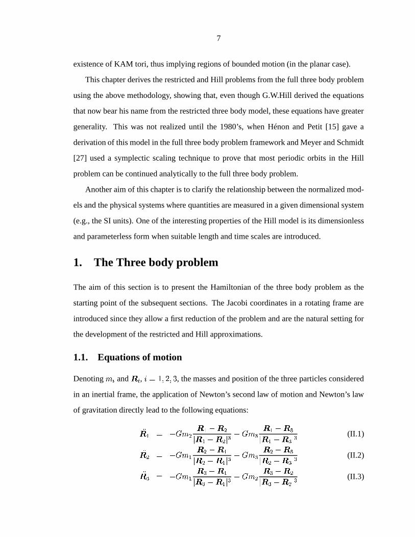
1.1. Equations of motion

Denoting and , , the masses and position of the three particles considered

in an inertial frame, the application of Newton’s second law of motion and Newton’s law

of gravitation directly lead to the following equations:

(II.1)

(II.2)

(II.3)

8

where represents the universal gravitational constant.

We can immediately see that, as , the first two equations reduce to a two body

problem, leaving the third equation describing the motion of a massless particle in the

gravitational field of two point mass particles. This is the restricted problem as formulated

in inertial space.

Similarly, as , the first two equations describe two uncoupled Keplerian

problems; this was the basis of Lunar theories before the work of Hill. A subtler scaling is

needed to take into account the coupling between the small masses.

1.2. Hamiltonian formalism and Jacobi coordinates

The Hamiltonian formalism is now introduced to investigate these limiting processes. We

rewrite the above differential equations as:

where

is the conjugate momentum of the position of the particle in the

inertial frame and the Hamiltonian

is given by:

! (II.4)

These equations admit the ten general integrals of motion present in the -body prob-

lem, namely, the energy, the position of the center of mass, the linear and angular momenta.

A change of coordinates can be used to eliminate the barycenter and linear momentum in-

tegrals. These coordinates, the Jacobi coordinates, are useful for deriving the restricted

and Hill model in the case of three bodies.

The first step in defining these coordinates is to transform the initial Hamiltonian (II.4)

into a rotating coordinate system with angular velocity

. That is, weIt is generally convenient to take "!#%$ , but this is not required at this stage.

9

make the following symplectic change of coordinates: where

(II.5)

so that for any vector

.

Under this change of coordinates, the above Hamiltonian transforms to :

!

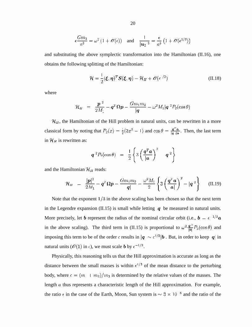
Then one can define the Jacobi coordinates as: " # # # # # #

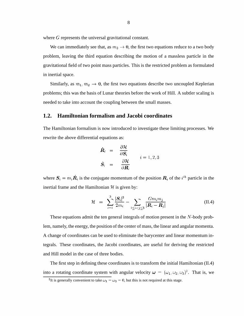
That is, the first vector, " , represents the position of the center of mass of the three

particles, the second vector, , represents the relative position of the second particle

relative to the first one, and the last vector, , corresponds to the position of the third

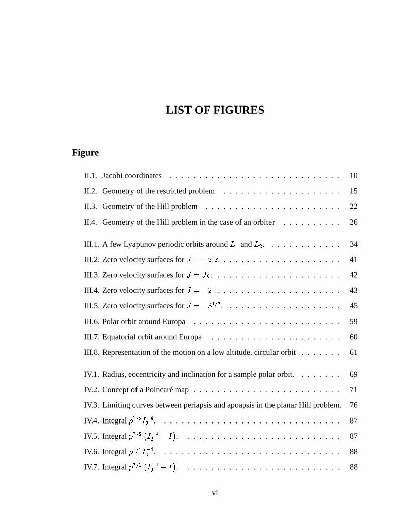
particle relative to the center of mass of the first two particles. Figure II.1 illustrates this

situation.

This point transformation can be made symplectic (see Appendix A) by defining: " # # ! # # # " # # See Meyer and Hall [26] or Arnold [3] for further details on time dependent canonical transformations.

10

Center of mass of the system

Center of mass of m1 and m2

m1

m2

m3

u0

u2

u1

Initial frame (Q’s)

Figure II.1: Jacobi coordinates

Then, the Hamiltonian reduces to

"

# (II.6)

where

" # #

#

# # #

and

#

#

Now the vectors " and " that represent the position and momentum of the center of

mass, are independent of the other variables in the Hamiltonian (they don’t appear in the

potential term) and one can reduce the Hamiltonian by setting " and " . This

corresponds to choosing the center of the frame at the center of mass of the system.

We are now ready to develop the different scalings that lead to the restricted and Hill

approximations.

11

2. The restricted approximation

The restricted three body problem describes the dynamics of a small mass attracted by two

point masses revolving around each other in a Keplerian circular orbit. This model has

found many applications in both astronomy and astrodynamics. It is indeed the simplest

model of the main perturbation of an object in interplanetary space (e.g., comet, Jupiter,

Sun system) or even for Earth orbiters for high enough altitudes [28].

2.1. Derivation

To derive this model from the Hamiltonian of the full three body problem (II.6), let the

mass of the third particle be denoted by . The Hamiltonian (II.6) is rewritten as:

#

(II.7)

where

(II.8)

and #

# # The Hamiltonian

represents a Kepler problem and depends only on and . Since the third mass is assumed to be small, it is physically legitimate to expect that

this particle will have very little effect on the motion of the first two masses. Therefore a

change of variable of the form and where represents a solution of the Hamiltonian (II.8) seems reasonable. We want however to

keep the autonomous nature of the system, and therefore, is chosen to be a

relative equilibrium (i.e., critical point) of the Kepler problem. These relative equilibria

correspond to circular orbits with mean motion equal to the angular velocity of the frame.

12

That is, we perform the following change of variable on : (II.9) (II.10)

where is orthogonal to and satisfies the relation

(see Appendix A):

# (II.11)

Then, one can develop around this nominal circular orbit by using Taylor’s

expansion theorem:

# #

where the constant term can be set to zero without loss of generality

since the addition of a constant in a Hamiltonian does not change the equations of motion.

represents the Hessian of evaluated at the critical point and is

equal to:

(II.12)

where represents the identity matrix.

That is, the term represents the linearized motion of the two particles

around a nominal circular orbit. This is the Clohessy-Wiltshire equations in Hamiltonian

form. These equations also appear in the derivation of the Hill problem (see next section)

and in the analysis of the motion far from the primary in the Hill approximation, as we

will see in the next Chapter. These equations will be studied in more detail at that point.

Returning to the Hamiltonian (II.7), one can complete the transformation (II.9)-(II.10)

into a canonical transformation with multiplier by setting: recall that vectors are represented by bold letters and the corresponding unbold letters represent their

norm. Here, and ! " .

13

Then, the Hamiltonian (II.7) transforms into:

# # (II.13)

where

# (II.14)

represents the Hamiltonian of the restricted problem. It only depends on and

.

Thus we see that an appropriate scaling allows us to rewrite the full three body problem

as the restricted problem plus a linear motion around a reference circular orbit, to the first

order in (i.e., ). That is, the motion of the primaries and the small mass particle

decouple to first order and one can study the motion of the small mass particle assuming

the primaries are fixed in the rotating coordinate system, i.e., and are taken equal to

zero.

Note that the above scaling does not change the length, mass and time scales with

which the original three body problem was formulated. The scaling only affects the

variable in the Hamiltonian of the restricted problem, but this scaling correspond to di-

viding by , which is a consequence of the uncoupling (to the first order) between the

and variables. Indeed, the equation of motion for particle in Newtonian

form does not depend the mass (see equations (II.1)-(II.3)). When the Hamiltonian

decouples, this independence appears directly in the Hamiltonian, in a similar fashion to

that in the Kepler problem (see Appendix A).

2.2. Normalization

In most studies of the restricted problem, the equations are written in a normalized form

where only one parameter, generally denoted , remains in the equations. This allows us,

for example, to perform numerical computation for a given value of and then apply the

results to any physical system which scales to this normalized model with this particular

value of .

14

To obtain this normalized form of the equations and the dependence of on the phys-

ical parameters, we change the length and time scale by using the following symplectic

transformation with multiplier :

where and need be chosen to simplify the Hamiltonian

.

Scaling of the time variable simply results in multiplying the Hamiltonian by the given

factor, here , so that the above scaling results in:

#

where has been obtained from the normalized vector .

Thus, we see that setting , and , results in nondimensional-

izing the Hamiltonian. Recall indeed that # , #

and # .Moreover, denoting , we have , and we obtain the normalized

Hamiltonian of the restricted problem written in vector form as:

# where

. The resulting equations of motion are given by:

# # #

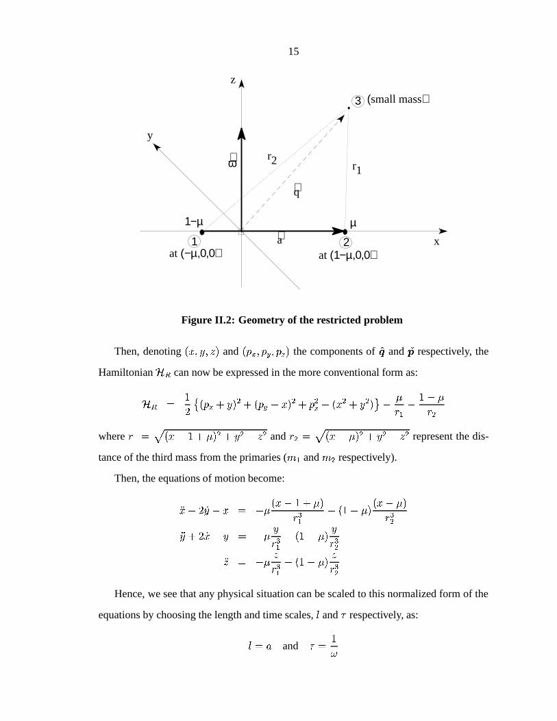
To express this Hamiltonian in Cartesian coordinates, it is standard to let and

, so that the -axis is chosen along the angular momentum of the primaries

and the primaries lie on the -axis. The -axis is chosen to complete the orthonormal frame

(see Figure II.2).

15

∼q

a

ω∼

∼ x

z

y

1−µ µ

1at (−µ,0,0)

2at (1−µ,0,0)

3 (small mass)

r1r2

Figure II.2: Geometry of the restricted problem

Then, denoting and the components of and

respectively, the

Hamiltonian

can now be expressed in the more conventional form as:

# # # #

where # # # and # # represent the dis-

tance of the third mass from the primaries ( and respectively).

Then, the equations of motion become:

#

#

Hence, we see that any physical situation can be scaled to this normalized form of the

equations by choosing the length and time scales, and respectively, as:

and

16

The only dimensionless parameter remaining in the equation, , is given by:

#

2.3. Comments

A more classical derivation of the restricted problem than that presented here can be found

in the treatise on the subject by Szebehely [37]. The above derivation was inspired by

Meyer [24, 25] and Meyer and Schmidt [27], even though the scaling used is not exactly

the same since the emphasis here was to make explicit the normalization process and the

length and time scales.

However, we should note that from the expression of the Hamiltonian derived in

(II.13), a further reduction of the Clohessy-Wiltshire part of the Hamiltonian results in the

following theorem, as a direct application of a standard perturbation theorem on Hamilto-

nian systems (see [24] for the full details):

Any non-degenerate periodic solution of the classical restricted problem

whose period is not a multiple of can be continued into the full three

body problem.

Also, we should note that the restricted problem is still of current research interest as

attested by the monographs of Hénon on families of periodic orbits [13], the papers on

homoclinic phenomena [22], or the studies on transport phenomena in the solar system

[21]. One of the main ingredients in this last subject only involves the dynamics close

to one of the primaries, and it can be analyzed using the Hill problem, as we shall see in

Chapter VI.

3. The Hill approximation

The Hill approximation can be used when two of the masses are close together and small

when compared to the third one. Hence, it is a complementary approach to the restrictedi.e., with multiplicity of the characteristic multiplier +1 exactly equal to 2.

17

case, even though the Hill approximation has traditionally been considered to be a special

case of the restricted problem and is often used in such a restricted sense. This special case

will be considered in the next section.

The general case is derived in this section using the same techniques as in the previous

section. In its full generality, the Hill problem has several applications in dynamical as-

tronomy, in particular in the exploration of planetary ring dynamics and binary encounters.

3.1. Derivation

As in the restricted problem, the derivation of the Hill problem from the full three body

problem results in splitting the Hamiltonian (II.6) into the linearized motion about a cir-

cular orbit and the Hamiltonian of the Hill problem to the first order in a small parameter

related to the smallness assumptions made on the masses and their mutual separations.

In the restricted problem, the third mass has been assumed small as compared to the

two others, thus it was physically reasonable to assume that the two remaining masses

were moving approximately on a Keplerian circular orbit.

Similarly, in the Hill approximation, we assume that the first two masses are small

compared to the third one (i.e., we assume and are small as compared to ) and

that the two small masses are close together as compared to their separation from the third

mass. Therefore, it seems physically reasonable to expect that the center of mass of the

two small masses will move on an approximate Keplerian orbit around , that is the

variables should appear in the Hamiltonian (II.6) as the Hamiltonian of a Kepler

problem to the zeroth order.

Since the terms in (II.6) that depends on are the last two terms, we can expand

them by using a Legendre polynomials. Recall indeed that for any vector and sucg

that ,

"

where represent the cosine of the angle between the vectors and and repre-

18

sents the Legendre polynomial of degree . These polynomials are given by the following

relations:

"

so that, and

.Now it is clear that the term # # can be expanded as:

"

(II.15)

where # " and represents the cosine of the angle between the

vectors and .Since

" # and , we see that the Hamiltonian (II.7) can be rewritten

as:

#

(II.16)

where

# (II.17)

and

We are now ready to apply the scaling that will introduce a small parameter: let represent the ratio , so that a small value of accounts for the smallness of the first

two masses as compared to the third one. Then, in order to take into account the first order

effects of this last large mass on the motion of and , we have to scale this effect

relative to this small parameter. More precisely, we want to scale the distance such that

the phase space region where the gravitational attraction of and on each other and

19

on are of the same order. That is, the smaller is , the farther the third mass must be

as compared to the separation of and . In such a situation, the combined effect of

and on is equivalent (to the first order in ) to the effect of a particle of mass

# that would be located at the center of mass of and . That is, follows

an approximate two body motion, as appears in , and a change of variable similar

to (II.9) and (II.10) for the variables is appropriate.

The following change of variables: " results in writing (II.17) as :

#

where, as previously, the constant term has been set to

zero without loss of generality. The matrix

is given by the same formula as in the case

of the restricted problem (formula (II.12)) but with replaced by and satisfying

the relation:

# #

Completing the above transformation by the identity transformation for the variables

, i.e.: one obtains a symplectic transformation of the original full three body problem.

Using the relations:See Appendix A for further details.

20

# and

#

and substituting the above symplectic transformation into the Hamiltonian (II.16), one

obtains the following splitting of the Hamiltonian:

# # (II.18)

where

, the Hamiltonian of the Hill problem in natural units, can be rewritten in a more

classical form by noting that and . Then, the last term

in

is rewritten as:

and the Hamiltonian

reads:

(II.19)

Note that the exponent in the above scaling has been chosen so that the next term

in the Legendre expansion (II.15) is small while letting be measured in natural units.

More precisely, let represent the radius of the nominal circular orbit (i.e., in the above scaling). The third term in (II.15) is proportional to

and

imposing this term to be of the order results in . But, in order to keep

innatural units ( in ), we must scale by .

Physically, this reasoning tells us that the Hill approximation is accurate as long as the

distance between the small masses is within of the mean distance to the perturbing

body, where # is determined by the relative values of the masses. The

length thus represents a characteristic length of the Hill approximation. For example,

the ratio in the case of the Earth, Moon, Sun system is and the ratio of the

21

Earth-Moon distance to the characteristic length is

. Thus, the Hill problem is

a good approximation to analyze the relative motion of the Earth and Moon as perturbed

by the Sun.

As for the restricted problem, we see that an appropriate scaling allows us to separate

the Hamiltonian of the three body problem, so that the motion of the two particles

and decouples from the motion of the distant, large mass . That is, to study the

motion of the masses and , one can assume the perturbing mass to be fixed in the

rotating frame (in the direction indicated by the vector from the center of mass of the

two small particles) and that its only effect is a linear perturbation (quadratic term in the

Hamiltonian) of a Keplerian problem in rotating coordinates. In fact, the need to formulate

the problem in a rotating frame is entirely due to the effect of this large mass.

Note that classically, the above scaling is described by saying that the perturbing mass

is at infinity and with an infinite mass. This accounts for the relations between the quan-

tities , , and when is taken to be zero in the above development. Of course, the

transformation obtained with such a value for is not symplectic!

3.2. Normalization

As for the restricted problem, the Hill problem can be normalized by selecting proper

length and time scales. Unlike the restricted problem, however, the normalized form of

Hill’s equations are parameterless, which allows us to scale any physical system modeled

by Hill’s equations into a unique “canonical” system.

We proceed similarly to the normalization of the restricted problem by introducing a

symplectic change of variable and time with free parameters ,

and :

and

Then the Hamiltonian (II.19) becomes:

22

where, as previously, tilde letters represent normalized quantities: and

is

obtain using (II.5) and .

Thus, we can see that choosing # , and ,

the Hamiltonian of the Hill problem normalizes to:

No parameters remain in this Hamiltonian and the equations of motion can be written

in vector form as:

# # #

∼

q

a

ω∼

∼

x

z

y1

m1

2

m2

3 (Large mass)

Center of mas ofm1 and m2

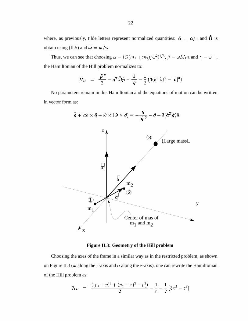
Figure II.3: Geometry of the Hill problem

Choosing the axes of the frame in a similar way as in the restricted problem, as shown

on Figure II.3 ( along the -axis and along the -axis), one can rewrite the Hamiltonian

of the Hill problem as:

# # #

23

where # # .

Then, the equations of motion can be rewritten in a standard form as:

# (II.20)

#

(II.21)

(II.22)

That is, this canonical form of the equations has been obtained by setting the length

and time scales and , respectively, to be:

#

3.3. Comments

In the derivation of the Hill problem in natural units, a preliminary symplectic scaling of

the momenta and allows us to write the Hamiltonian of the Hill

problem (II.19) without the dependence on :

# (II.23)

This reflects the fact that the scaling allows us to decouple the motion of the third particle,

and as a result the relative position of the first two masses depends only on the total mass

# of the system ( indeed represents the relative position of and ), in a

similar manner as for the Kepler problem. This scaling does not affect the units of length,

time and mass.

Another derivation of the Hill problem from the full three body problem can be found

in Hénon and Petit [15]. The above derivation has been inspired by the papers of Meyer on

symplectic scaling and periodic orbits [24, 25] and Meyer and Schmidt [27]. The scaling

adopted here differs from that used in [27], however, since, as for the restricted problem,

our aim was to keep the natural units of length and time throughout to make explicit the

24

relationship between the normalized equations and the physical systems modeled by these

equations. We should note, however, that a further reduction of the Clohessy-Wiltshire

part of the Hamiltonian (II.18) results in an analogous theorem to the one quoted for the

restricted problem (see [27] for the full details):

Any non-degenerate periodic solution of Hill’s equations whose period is

not a multiple of can be continued into the full three body problem.

Besides the study of families of periodic orbits [12], the Hill problem has been investi-

gated by several researchers who studied chaotic scattering [17, 12] and the destruction of

KAM tori [36]. It is interesting to note, indeed, that a linear perturbation of an integrable

problem may result in a non-integrable one.

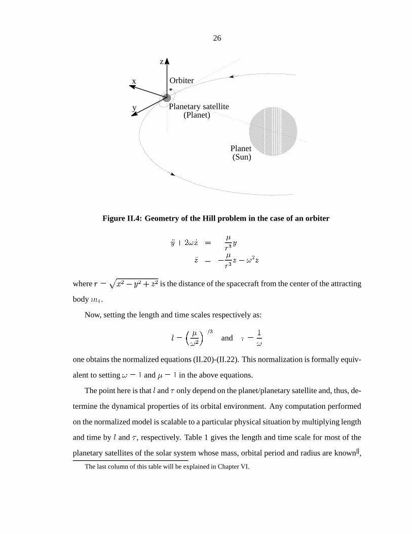
4. The orbiter case: The restricted Hill problem

When the the mass is small compared to in the above Hill problem, one can further

expand the Hamiltonian (II.23) so that the center of the frame is located at the center of

mass of the first body, , and the resulting problem becomes independent of the small

mass (to the first order in this small parameter). This further approximation is the

same as the one performed in the restricted two body problem (see appendix A) where a

spacecraft moving around the Earth is analyzed with an “inertial” frame fixed at the center

of the Earth.

The restricted Hill problem can represent the motion of an orbiter around a planet or

planetary satellite as perturbed by the Sun or a massive planet respectively.

4.1. The restricted Hill problem

We start from the Hill problem as defined by (II.23). Note that, in this problem, the center

of the frame is at the center of mass of and . Now, assuming the second mass small

as compared to the first one, we let and the Hamiltonian

is rewritten as:

#

25

where

(II.24)

This Hamiltonian

is formally the same as

with the mass # replaced

by the mass , and, upon applying the normalization:

the restricted Hill problem transforms into the same normalized form of the equations as

the Hill problem (II.20)-(II.22).

Note here, however, that the Kepler part of the Hamiltonian

corresponds to a

restricted two body problem with center of mass fixed at the origin of the rotating

frame. This is indeed the case since, in this approximation, # , so

that # is defined relative to the center of mass of the first body .

Figure II.4 illustrates this situation.

4.2. Scaling to planetary satellites

The Hamiltonian

is independent of the mass of the spacecraft, , and only depends

on the properties of the central planet/planetary satellite, . These properties are the

gravitational parameter, , and the orbital angular velocity, , around the large,

perturbing mass. The parameter governs the two body effects of the motion while

governs the third body effects. Setting reduces the Hamiltonian

to a restricted

two body problem.

Expressed in natural units, the equations of motions of the spacecraft are:

#

26

x

y

z

Orbiter

Planetary satellite (Planet)

Planet (Sun)

Figure II.4: Geometry of the Hill problem in the case of an orbiter

#

where # # is the distance of the spacecraft from the center of the attracting

body .

Now, setting the length and time scales respectively as:

and

one obtains the normalized equations (II.20)-(II.22). This normalization is formally equiv-

alent to setting and in the above equations.

The point here is that and only depend on the planet/planetary satellite and, thus, de-

termine the dynamical properties of its orbital environment. Any computation performed

on the normalized model is scalable to a particular physical situation by multiplying length

and time by and , respectively. Table 1 gives the length and time scale for most of the

planetary satellites of the solar system whose mass, orbital period and radius are known ,The last column of this table will be explained in Chapter VI.

27

allowing one to scale the subsequent computations to any particular physical system mod-

eled by the Hill equations. In the remainder of this dissertation, computations will be

performed in the non-dimensional setting, with some scaled results given for the sake of

illustration.

Finally, we should note that these scalings depend both on the physical parameters of

the primaries as well as their orbital characteristics (mean motion ). Therefore, planetary

satellites of rather different mass and radius may have the same normalized radius, as is

approximately the case for Io (Jupiter), Dione (Saturn) and Ariel (Uranus) (see Table 1).

Similarly, planetary satellites with similar physical radii can have very different dynamical

properties, and thus a large difference in their normalized radius, as for example with the

Jupiter satellites Amalthea and Himalia. As we will see in the next chapter, low altitude,

stable circular orbits around Himalia are possible while their existence is doubtful for the

case of Amalthea.

4.3. From the restricted to the Hill problem

The restricted Hill problem has been derived from the Hill problem by assuming that the

second mass was small as compared to the first one. The same situation can occur in the

restricted three body problem, thus leading to the same problem.

This subsection indicates how to derive the restricted Hill problem from the restricted

three body problem in order to complete the description of the relationship between the

Hill and the restricted problems. Moreover, this point of view was the original one adopted

by Hill in his “Researches in the Lunar theory” [18]. Starting from the Hamiltonian of

the restricted problem (II.14) and applying the following symplectic change of variables:

#

Though he did not use the Hamiltonian formalism.

28

one obtains the following Hamiltonian:

# #

where the constant term has been removed from the Hamiltonian since

it does not change the equations of motion.

Then, one can expand the term in a similar way as for the derivation of the Hill

problem:

#

# #

where, as previously,

represents the Legendre polynomial of degree and is the

cosine of the angle between the vectors and .

Letting , the relations between and

can be written as:

# and # so that: # and, upon removing the constant terms, one obtains the following Hamiltonian:

# As for the Hill problem, we can let (where

is assumed to be of the

same order as , consistent with the assumption that the disturbing body is far from the

primary ), so that the above Hamiltonian reduces to the Hamiltonian of the restricted

Hill problem to the first order in . (Note that the notation is different from the restricted

Hill problem as given by (II.24). Here, the disturbing body is and the spacecraft is

represented by and the characteristic length is given by ).

See equations (II.11) and Appendix A.

29

4.4. Comments

The terminology “restricted Hill problem” is not used in standard practice and no distinc-

tion is generally made between the Hill problem and its restricted form. These models are

indeed represented by the same sets of equations, even though the length scales are slightly

different. This situation is, in fact, the same as for the two body problem (see Appendix

A) and thus the common usage will be used in the remainder of this dissertation.

As we have seen in this section, the Hill and restricted problems are not incompatible

and the orbiter case represents a physical situation that can be modeled by either of these

models. However, as indicated in the introduction, the Hill problem has the non-negligible

advantage of simplicity.

These two models can also be obtained for the four body problem where the restricted

and Hill approximations can be used in conjunction to model the motion of a spacecraft in

the Earth-Moon environment, as perturbed by the Sun [30].

CHAPTER III

DYNAMICS OF THE HILL PROBLEM

This chapter presents some features of the dynamics in the Hill problem that are used in the

subsequent chapters. The results are presented in the normalized form of the Hill problem,

as given by equations (II.20)-(II.22).

The first section presents the basic properties of Hill’s equations, such as the invariance

of the equatorial plane, the equilibrium solutions and the symmetries present in this prob-

lem. This last property is especially useful in numerical investigations since it generally

reduces (by at least a factor of four) the regions of phase space to be analyzed.

The second section investigates the implications of the Hamiltonian nature of the Hill

problem, by presenting the basic topology and geometry of the energy manifold. The key

points consist of the existence of a minimum threshold in the value of the Hamiltonian

before escape becomes possible, and a maximum value of energy for which all transit

trajectories will have a closest approach to the primary (i.e., periapsis passage).

The third section presents the reformulation of the Hill problem in terms of orbital

elements. This formulation will be used in the following chapters. Orbital elements rep-

resent the most commonly used set of variables in celestial mechanics and astrodynamics

and many properties are easily expressed in terms of them. In particular, all the results

obtained in terms of orbital elements can be compared to a two body model, where these

elements are constants of the motion. This section also presents the Delaunay variables,

which can be though of as a canonical representation of the elements.

While the nonlinear dynamics of interest to us are on the order of the length and time

30

31

scale of the Hill problem, dynamics close to and far from the primary are given attention as

they contain some of the features needed in the orbit transfers considered later. Also, these

dynamics represent a link between two commonly used models in spacecraft trajectory

analyses, the Kepler and restricted three body problems.

In particular, the investigation of dynamics close to the primary, presented in Section, allows us to establish the existence of stable, low altitude, circular orbits. Motion of

a spacecraft can then be approximated by a Keplerian circular orbit when close to the

primary, for relatively short time spans. The presentation uses both a symplectic technique,

allowing us to reduce the Hamiltonian of the Hill problem into a Kepler problem to the

first order in a small parameter and to prove the existence of KAM tori, and an averaging

approach.

Finally, a brief analysis of motion far from the primary is performed using the Clohessy-

Wiltshire equations. These dynamics are related to the restricted problem in the case of

an orbiter. These dynamics can be considered as an outer layer between the Hill and the

restricted problem and can be used to patch the results obtained from the escape problem

to a restricted model.

Note that this chapter is not exhaustive and only presents the properties that are relevant

for the subsequent results. Many topics of interest in the Hill problem are not mentioned

in this chapter.

1. First properties

Recall that the normalized Hill problem is given by the equations:

# (III.1)

#

(III.2)

(III.3)

32

where # # is the magnitude of the relative position vector between the

small masses. The rotating frame in which these equations are formulated has been pre-

sented in Figure II.4 for the case of an orbiter.

Looking at these equations, we see that the only out-of-plane force acting on the par-

ticle is proportional to its altitude over the equatorial plane (i.e. the -plane). Thus,

if at any given instant one has and , the particle will remain in the equatorial

plane for all times. That is, the equatorial plane is invariant under the flow and one can

consider the Hill problem to be restricted in this plane, as was done in the original paper

by Hill [18]. As we will see subsequently, the dynamics in the planar case and in the spa-

tial problem are somewhat different, and generally easier in the planar problem. However,

both cases are of interest and we will consider both of them in the sequel.

1.1. Libration points

The next, almost obvious, property of the Hill problem is the existence of equilibrium

solutions. These can be determined by setting all the derivatives to zero in the above

equations and solving for the remaining variables, or by computing the critical points of

the Hamiltonian (II.20).

These equilibrium solutions are located on the -axis at

. The point with

negative abscissa is generally denoted and the one with positive abscissa is denoted .

We will denote

in the sequel. These solutions are called the libration points

because of the existence of periodic and quasi-periodic orbits in their vicinity.

Indeed, the linearized equations around these points are given by:

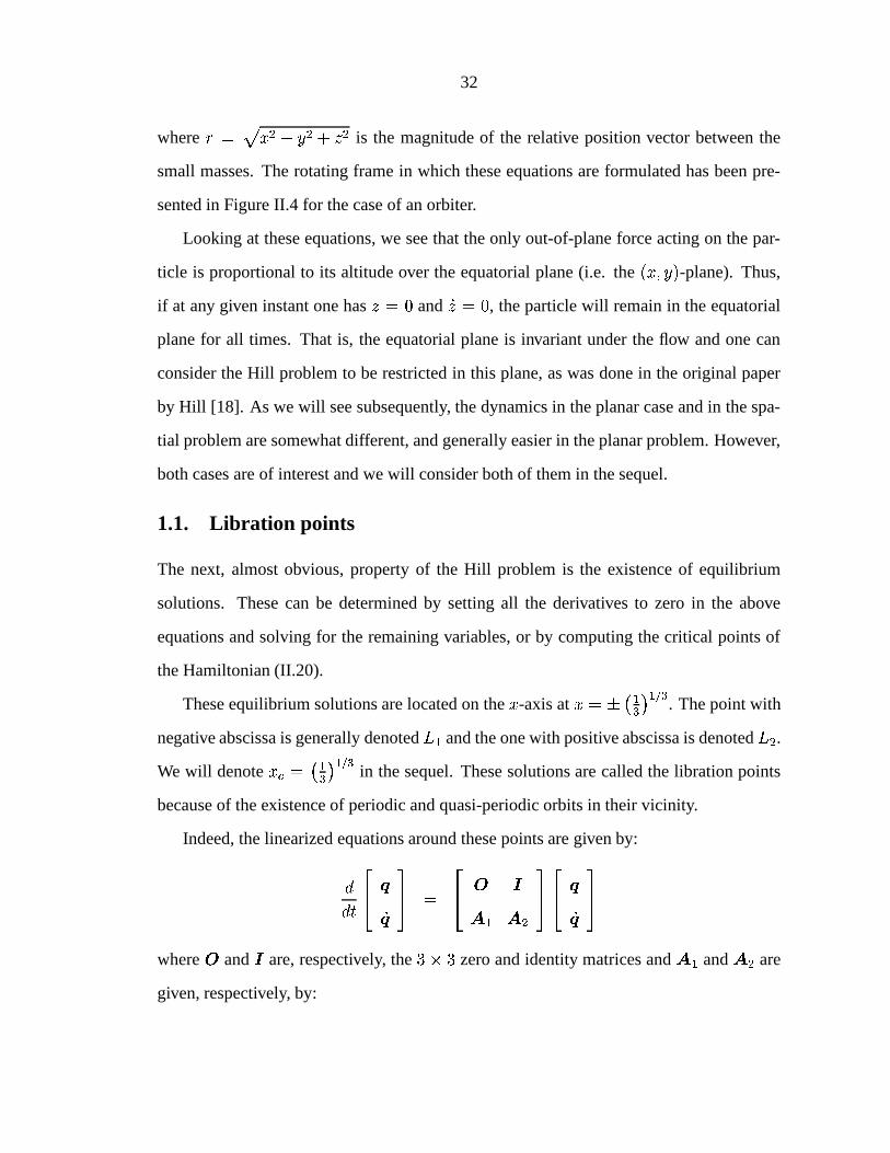
where

and are, respectively, the zero and identity matrices and and

are

given, respectively, by:

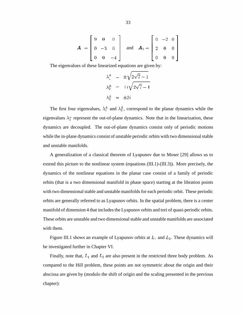
33

and

The eigenvalues of these linearized equations are given by:

#

The first four eigenvalues, and

, correspond to the planar dynamics while the

eigenvalues represent the out-of-plane dynamics. Note that in the linearization, these

dynamics are decoupled. The out-of-plane dynamics consist only of periodic motions

while the in-plane dynamics consist of unstable periodic orbits with two dimensional stable

and unstable manifolds.

A generalization of a classical theorem of Lyapunov due to Moser [29] allows us to

extend this picture to the nonlinear system (equations (III.1)-(III.3)). More precisely, the

dynamics of the nonlinear equations in the planar case consist of a family of periodic

orbits (that is a two dimensional manifold in phase space) starting at the libration points

with two dimensional stable and unstable manifolds for each periodic orbit. These periodic

orbits are generally referred to as Lyapunov orbits. In the spatial problem, there is a center

manifold of dimension 4 that includes the Lyapunov orbits and tori of quasi-periodic orbits.

These orbits are unstable and two dimensional stable and unstable manifolds are associated

with them.

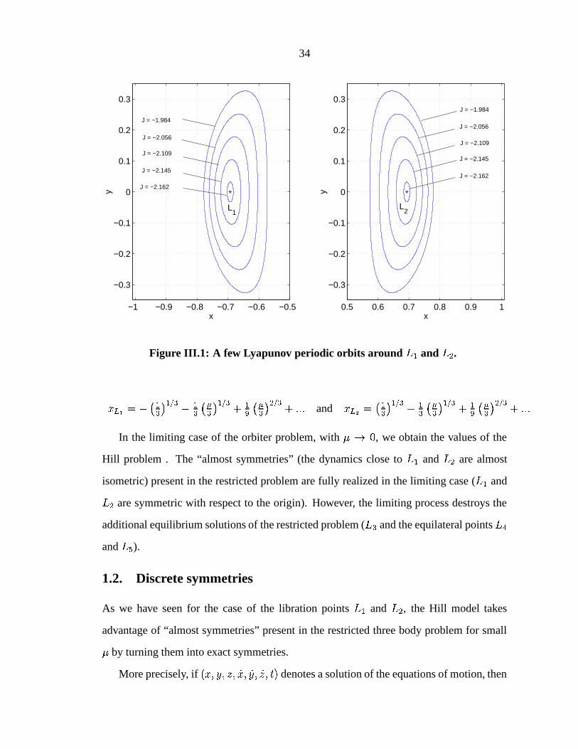
Figure III.1 shows an example of Lyapunov orbits at and . These dynamics will

be investigated further in Chapter VI.

Finally, note that, and are also present in the restricted three body problem. As

compared to the Hill problem, these points are not symmetric about the origin and their

abscissa are given by (modulo the shift of origin and the scaling presented in the previous

chapter):

34

−1 −0.9 −0.8 −0.7 −0.6 −0.5

−0.3

−0.2

−0.1

0

0.1

0.2

0.3

L1

x

yJ = −1.984

J = −2.056

J = −2.109

J = −2.145

J = −2.162

0.5 0.6 0.7 0.8 0.9 1

−0.3

−0.2

−0.1

0

0.1

0.2

0.3

L2

xy

J = −1.984

J = −2.056

J = −2.109

J = −2.145

J = −2.162

Figure III.1: A few Lyapunov periodic orbits around and .

#

# and #

#

#

In the limiting case of the orbiter problem, with , we obtain the values of the

Hill problem . The “almost symmetries” (the dynamics close to and are almost

isometric) present in the restricted problem are fully realized in the limiting case ( and

are symmetric with respect to the origin). However, the limiting process destroys the

additional equilibrium solutions of the restricted problem ( and the equilateral points and ).

1.2. Discrete symmetries

As we have seen for the case of the libration points and , the Hill model takes

advantage of “almost symmetries” present in the restricted three body problem for small

by turning them into exact symmetries.

More precisely, if denotes a solution of the equations of motion, then

35

the trajectories obtained by applying the following transformations are also valid solutions:

The compositions of these three symmetries yield other symmetries, notably the composi-

tions of (1),(2) and (1),(2),(3) yield:

This last symmetry is a pure symmetry about the origin which results in the symmetry

of and . More generally, all the dynamics that are present in the vicinity of are

also present in the vicinity of , and the corresponding trajectories are symmetric about

the origin. This is the case for the Lyapunov orbits, as is clearly apparent on Figure III.1,

and for the stable/unstable manifolds of these periodic orbits. In other words, if is

a property of a trajectory close to , then will be the corresponding property

of the symmetric trajectory in the vicinity of . This will apply to the case of escaping

trajectories as discussed in Chapter VI, where the one-to-one correspondence between

and will allow us to restrict the analysis to -escaping trajectories.

From , we see that the same is true for reflections about the -plane, allowing

us, in the case of escaping trajectories, to restrict the computations to trajectories having a

positive -coordinate. This will be used to simplify the computation of the Poincaré maps.

The symmetries and involve a reflection in time, and applied to the case of the

dynamics close to the libration points, we see that the stable and unstable manifolds are

symmetric about the -plane. Again, this can be seen on Figure III.1. In the case of

escaping trajectories, applying and results in capture trajectories, and the analysis

performed in Chapter VI will directly apply to this class of trajectories. Further discussion

of these cases will be considered then.

36

Thus, we see that the many symmetries present in the Hill problem can significantly

simplify the computation and analysis for preliminary studies, and allows us to see the

similarities between several classes of trajectories which are otherwise different in the

setting of the restricted three body problem.

2. The Jacobi constant and the energy manifold

We have seen in the previous chapter that the Hill problem can be written in normalized

form as a Hamiltonian system with Hamiltonian given by:

(III.4)

(tildes have been removed, as compared to equation (II.20), for notational convenience).

Since this Hamiltonian is independent of time, it is conserved along the flow defined

by the equations of motion. This integral of motion, written in position/velocity form, is

know as the Jacobi constant and is denoted .

#

Written in Cartesian coordinates, this integral takes the form:

(III.5)

where # # represents the speed of the spacecraft in the rotating

frame and # # represents its distance from the center of the primary.

2.1. The energy manifold and zero velocity surfaces

The existence of this integral of motion has an immediate consequence. At a fixed value

of , motion is constrained to lie on the energy manifold , which is five dimensional in

the spatial problem and three dimensional in the planar problem. The manifold can beThis name is sometimes given in the literature to the quantity . Note that .

37

expressed in position/velocity form as:

Notably, the projection of onto position space, called the Hill region, can have a

bounded component, thus implying bounded regions of motion. This region is denoted

:

In order to investigate the topology and geometry of these regions, let us first remark

that the boundaries of and

are the same and correspond to the surfaces of zero

velocity, , defined by setting in the definition of .

# #

#

Away from these surfaces, the pre-image of a point under the natural projection of

over

is a two-sphere representing all possible directions of the velocity vector at that

position. Indeed, the dependence of on is only through its magnitude, , so that for

a given value of the Jacobi constant and a given position, the magnitude of the velocity

vector is fixed.

Thus we see that the topology of the energy manifold and Hill regions are really de-

termined by the surfaces of zero velocity. The topology of these surfaces change at the

critical points of the Jacobi constant when is set to zero:

#

Thus, we see that

for

, , that is the first singularity

in the zero velocity surfaces occurs at the libration points and . These critical points

occur for a value of equal to and it can be checked that they are non-

degenerate with index two. In the compact case, Morse theory indicates that the topology

38

of the surface for and differs by a two-cell. In our case, the surfaces are

non-compact but, as we see below, a similar situation occurs. More precisely, for ,

has three different connected components, one of which (the closest to the primary) is

bounded. For , the two unbounded components connect with the bounded one by

forming two “throats” that allow particles to move from the inner side of the primary’s

orbit to its outer side. The subsection below investigates this change in more detail.

The second singularity of the zero velocity surface is obtained when and

. As we see below, this case does indeed correspond to a change in the topology

of the surfaces, even though the singularity is degenerate. In this case, and the zero

velocity surfaces detach from the -plane.

2.2. A closer look at the zero velocity surfaces

In order to obtain a more precise picture of these zero velocity surfaces, it is convenient to

rewrite the defining relation in spherical coordinates, as defined by:

so that , is the longitude (

) and

is the latitude ( ).

Then the relation # # # is rewritten as (after

multiplication by ):

# ! # (III.6)

where . This equation is a reduced cubic

equation in and an explicit solution is available through the use of Cardan’s formulas (see

Appendix C).

Note that on the planes . From equation (III.6), we deduce that

the zero velocity surfaces will intersect these planes at a fixed distance from the

39

origin. These intersections will only exist for . The projection of these intersections

on the -plane corresponds to ellipses of semi-major axis equal to along the -axis

and semi-minor axis equal to along the -axis.

When the zero velocity surfaces do not intersect these planes, nor do they

restrict motion in the equatorial plane (i.e., the -plane). Indeed, the discriminant of

the reduced cubic (III.6) is:

#

!

so that

when . This implies the existence of a single real root of the

equation, but Descartes’ rule (see Appendix C) indicates that this root is negative (i.e.,

there is no solution since represents a distance and is, by definition, positive). Thus,

there is no component of the zero velocity surface in the region when .

Now, from the definition of , it is clear that , with on the -axis and on the -axis. Thus, this short discussion shows that for

, the zero velocity surfaces do not cross the equatorial plane and only restrict the

out-of plane motion.

Since the applications where the zero velocity surfaces enter into play (chapter VI)

only involve low energies ( ), the remainder of this discussion will focus on this case.

Appendix C contains further material on the case .

When and (polar region), it is clear that

and, by Descartes’

rule, the only real solution of (III.6) is positive. Hence, in the polar region, the zero

velocity surfaces intersect the radial lines at only one point. This solution tends to

as .

For , three cases have to be considered:

When , and Descartes’ rule can be used to show that there are

exactly two distinct positive solutions of (III.6) for each and

. By examining

these solutions (see Appendix C), one can see that the smallest solution connects to

40

the polar cap at on the planes , and the other solution to # as

. Hence, for , the zero velocity surfaces have one bounded

component near the primary and two unbounded components further apart. Motion

in the bounded component is, per force, bounded, and particles close to the primary

cannot escape. Figure III.2 gives a graphical representation of this case.

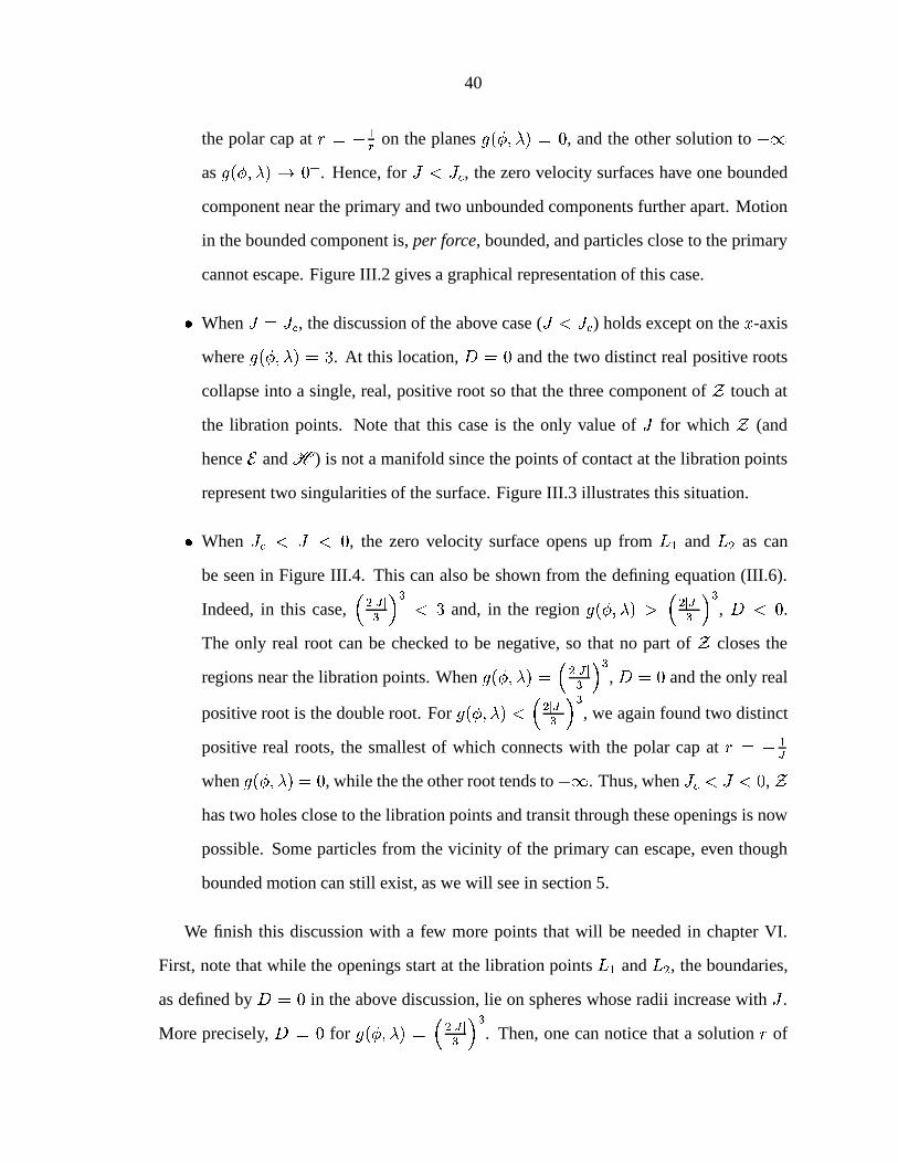
When , the discussion of the above case ( ) holds except on the -axis

where . At this location, and the two distinct real positive roots

collapse into a single, real, positive root so that the three component of touch at

the libration points. Note that this case is the only value of for which (and

hence and

) is not a manifold since the points of contact at the libration points

represent two singularities of the surface. Figure III.3 illustrates this situation.

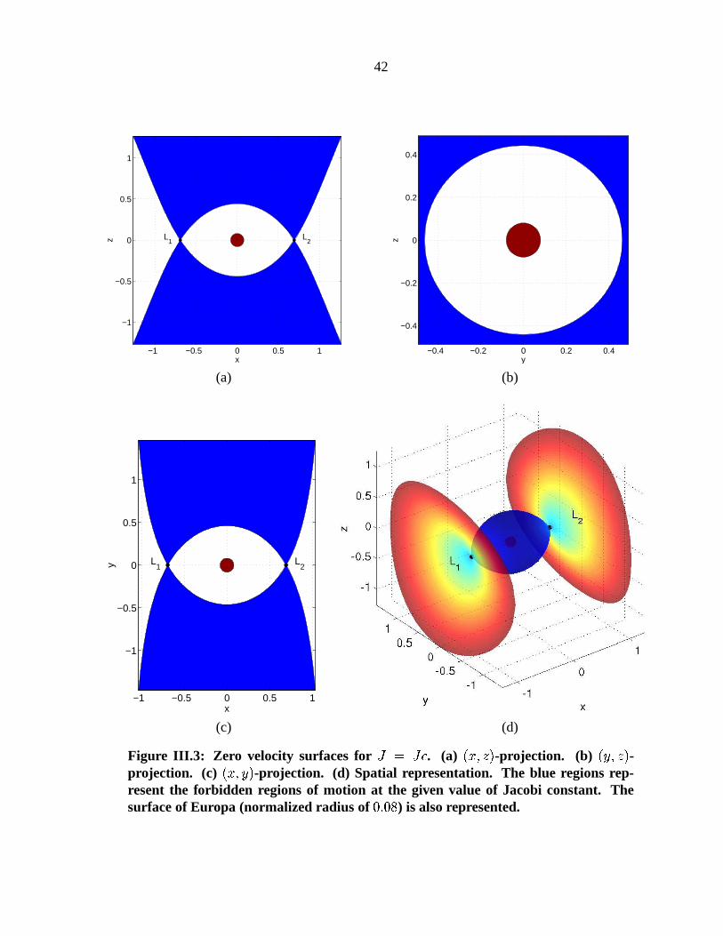
When , the zero velocity surface opens up from and as can

be seen in Figure III.4. This can also be shown from the defining equation (III.6).

Indeed, in this case, and, in the region , .

The only real root can be checked to be negative, so that no part of closes the

regions near the libration points. When , and the only real

positive root is the double root. For , we again found two distinct

positive real roots, the smallest of which connects with the polar cap at

when , while the the other root tends to # . Thus, when ,

has two holes close to the libration points and transit through these openings is now

possible. Some particles from the vicinity of the primary can escape, even though

bounded motion can still exist, as we will see in section 5.

We finish this discussion with a few more points that will be needed in chapter VI.

First, note that while the openings start at the libration points and , the boundaries,

as defined by in the above discussion, lie on spheres whose radii increase with .

More precisely, for . Then, one can notice that a solution of

41

L1

L2

x

z

−1 −0.5 0 0.5 1

−1

−0.5

0

0.5

1

y

z

−0.5 0 0.5

−0.4

−0.2

0

0.2

0.4

(a) (b)

L1

L2

x

y

−1 −0.5 0 0.5 1

−1

−0.5

0

0.5

1

(c) (d)

Figure III.2: Zero velocity surfaces for . (a) -projection. (b) -projection. (c) -projection. (d) Spatial representation. The blue regions rep-resent the forbidden regions of motion at the given value of Jacobi constant. Thesurface of Europa (normalized radius of ) is also represented.

42

L1

L2

x

z

−1 −0.5 0 0.5 1

−1

−0.5

0

0.5

1

y

z

−0.4 −0.2 0 0.2 0.4

−0.4

−0.2

0

0.2

0.4

(a) (b)

L1

L2

x

y

−1 −0.5 0 0.5 1

−1

−0.5

0

0.5

1

(c) (d)


43

L1

L2

x

z

−1 −0.5 0 0.5 1

−1

−0.5

0

0.5

1

y

z

−0.5 0 0.5−0.5

−0.4

−0.3

−0.2

−0.1

0

0.1

0.2

0.3

0.4

0.5

(a) (b)

L1

L2

x

y

−1 −0.5 0 0.5 1

−1

−0.5

0

0.5

1

(c) (d)


44

(III.6) depends on and

only through the function , so that, at constant , is constant.

In the case , one can check that

, that is, the openings, as

defined by tangency with the radial line, correspond to the intersection of the zero velocity

surface with a sphere of radius that increases with (since we only consider the

case ).

However, one can also define the openings as the minimum area sections of the throats.

Since the zero velocity surfaces start from the -axis and is symmetric about the and

plane, these minimum area sections are delimited by the points of at which the

distance from the -axis is minimal. This distance, # , can be obtained from

the definition of (equation (III.5)) as:

# !

(III.7)

Upon computing , one can check that the minimum is reached at:

# for

for

Then, and one can compute to be exactly . That is, while

the openings as defined by tangency with the radial lines lie on spheres whose radii, , increase with , the minimum area sections lie on a fixed sphere with radius ,

independent of .

Further computations of derivatives (see Appendix C) allow us to show that the mini-

mum distance of the zero velocity surfaces from the origin (tangent spheres) are reached

at the poles for the spatial problem and on the -axis in the planar problem at .

This last value is always greater than the radius obtained at the poles. Moreover, since

for , we see that every transit trajectory (i.e., a trajectory crossing

the planes and ) must have a point of closest approach from the primary

inside the region bounded by the planes (i.e., the existence of a periapsis passage

as defined by and

is guaranteed). Figure III.5 illustrates the geometry of the

zero velocity surface for the critical value of .

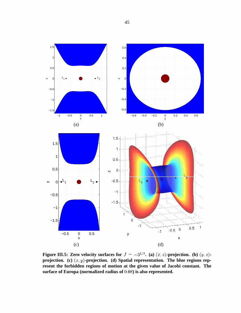
45

L1

L2

x

z

−1 −0.5 0 0.5 1

−1.5

−1

−0.5

0

0.5

1

1.5

yz

−0.6 −0.4 −0.2 0 0.2 0.4 0.6

−0.6

−0.4

−0.2

0

0.2

0.4

0.6

(a) (b)

L1 L

2

x

y

−0.5 0 0.5

−1.5

−1

−0.5

0

0.5

1

1.5

(c) (d)


46

Finally, we should like to note that in the same way as has been derived from the

definition of the Jacobi integral (III.5), we readily obtain that satisfies:

# ! (III.8)

thus showing that the zero velocity surfaces are asymptotic to the surfaces # ! .

3. Orbital elements and Delaunay variables

Orbital elements are ubiquitous in both celestial mechanics and astrodynamics. They rep-

resent a convenient and geometric way of parameterizing the state of a point mass particle,

and much useful information can be easily extracted from them.

This subsection recalls the definition of the orbital elements while emphasizing a slight

modification that is well suited for problems formulated in a rotating frame, as is the case

with the Hill problem.

3.1. Orbital elements

The Kepler problem is completely integrable and the path of any particle consists of a conic

section whose nature depends on the value of the energy (ellipses, parabolas or hyperbolas

for negative, zero or positive energies, respectively). Even though the orbital elements are

defined for all regimes of motion, we are mainly interested in motion presenting several

periapsis passages, so our focus will be on the elliptical case.

The shape of the ellipse in the orbital plane is either described by the semi-major axis,

, and the eccentricity, , or the periapsis and apoapsis radii, and , respectively. These

quantities are related via and # . Then, motion on the ellipse

is described by an angular coordinate that is related to the time, as for example the true

anomaly, , the eccentric anomaly, , or the mean anomaly, . These quantities are

related to each other via:

#

47

This last equation is Kepler’s equation and cannot be solved algebraically. The mean

anomaly is then related to time via " where

is the mean motion

and " represents the time of periapsis passage.

Then in order to complete the description of the state of a particle, one must determine

the position of the ellipse in space, through, for example, the use of three Euler angles

(the sequence from an initial Cartesian frame) known as the longitude of the

ascending node,

, the inclination, , and the argument of periapsis, .

Note that, even though orbital elements are very useful, they are not well defined for

zero eccentricity and zero inclination ( and

are not well defined in these cases). Other

sets of elements have been devised for these cases, but we will not use them in this work.

The relation between the Cartesian coordinates of an inertial frame and the orbital

elements can be expressed as:

(III.9)

where is the direction cosines matrix of the ellipse

in space and , the magnitude of the position vector, satisfies # .

The definition of the orbital elements given above allows us to easily express the mo-

tion of a point particle in a central gravitational field since, in this case, are

constants of motion.

Now, when the field is no longer central, the orbital elements vary as a function of

time, but can still be used as a parameterization of the phase space and often represent a

convenient system of coordinates (even though they are not canonical). Lagrange proposed

an easy way to obtain the differential equation governing these variations. The resulting

equations are now known as the Lagrange planetary equations and can be expressed as:

"!Recall that we are in a non-dimensional setting where the gravitational parameter # is equal to $ .&%('

and% represent the rotation matrices about the third and first axis respectively.

48

where represents the vector of orbital elements, represents a

matrix whose elements are given by the Lagrange brackets (

for any element and ) and !

represents the gradient of the negative

of the Hamiltonian (as expressed in an inertial frame, i.e., kinetic plus potential energy)

with respect to the elements. It is customary to remove the Keplerian energy part of!

,

i.e., , and call the resulting function the disturbing function, denoted

. Since only

the equation governing the variations of the mean anomaly depends on , Lagrange’s

planetary equations can be expressed with

in place of!

, except for the mean anomaly

equation to which has to be added.

3.2. Formulation in a rotating frame

Note that the above definition of the orbital elements are defined specifically relative to

an inertial frame. However, as soon as the center of the frame is at the center of mass of

the primary, any inertial frame can be used. In particular, when a problem is formulated

in a rotating frame, as is the case for the Hill problem, one can define the elements at

each instant of time in the inertial frame that is superimposed with the rotating frame at

that instant. This is equivalent to defining the longitude of the ascending node relative

to the -axis of the rotating frame. Indeed, since at two different instants and the

corresponding inertial frames only differ by a rotation around the -axis with angle , the only difference in defining the elements in the two frames lies in the longitude of

the ascending node which is shifted by . Thus, setting an initial inertial frame

that is superimposed with the rotating frame at the initial epoch , one obtains the

relation:

" We denote the angular speed of the frame to make its dependence explicit and reserve the notation

(that was used in Chapter II) only for the argument of periapsis so as to avoid any confusion. Note that inthe normalized setting, $ .

49

where

represents the longitude of the ascending node in the rotating frame and " is the

longitude of the ascending node with respect to the given, initial inertial frame.

Now, to obtain the variations of the elements in the rotating frame, we can simply note

that and

for any function

. Thus, the Lagrange brackets are

the same in the inertial and rotating frame, and the Lagrange planetary equations for the

rotating frame are simply obtained by adding to the right hand side of the equations

governing " .

However, a more fundamental way to view this point is to realize that the derivation of

Lagrange’s planetary equations are valid for any set of first order differential equations

and any valid set of elements (i.e., a change of variables that must be one-to-one). The

only difficulty being the computation of the brackets.

In particular, this derivation is very well suited for a canonical set of equations. Starting

from and

, one can express the left hand sides in terms of the elements

:

(III.10)

(III.11)

so that, multiplying (III.10) by and (III.11) by

and adding the results, one

obtains:

where, as previously, has its components given by the Lagrange brackets:

(III.12)

Upon inverting , one obtains the Lagrange planetary equations for any Hamiltonian

system.

In the case of the Kepler problem in a rotating frame,

so that

# and, thus,

represents the velocity in inertial space. Then, from (III.12), it

50

is immediately clear that the brackets computed in the rotating frame are exactly equal to

the brackets computed in the inertial frame, which are superimposed on the rotating frame

for each given instant. Moreover, the Hamiltonian of the Kepler problem in a rotating

frame is expressed as a Kepler problem in an inertial frame plus the disturbing function

where

is the angular momentum (per unit mass) of the particle in

inertial space. Thus we see that the Lagrange planetary equations for a problem formulated

in a rotating frame are the same as the classical Lagrange planetary equations with the

addition of a term

, that depends on the angular momentum in the disturbing function.

In the case of the Hill problem, the disturbing function is (without the addition of

):

so that, using the relations between Cartesian and orbital elements, one obtains:

# #

where

is defined with respect to the -axis of the rotating frame.

3.3. The Delaunay variables

The orbital elements are very convenient for many purposes but are not canonical, and

a canonical set of elements may thus be desirable when one wants to apply theorems

that are formulated in a canonical framework, such as the existence of KAM tori. One

such possible set of elements was derived by Delaunay and consists of complementing the

elements , and

by three variables, denoted , and .

Noting that Hamilton’s equations can be written as:

where and is the symplectic matrix and comparing them with the Lagrange

planetary equations as expressed for a Hamiltonian system:

where

and

are, respectively, the zero and identity matrices.

51

we see that the elements will be canonical if and only if (indeed, ).

This is equivalent to imposing normalized conditions for the brackets, as given by:

From the classical expression of the brackets in terms of , it is easy to

check that , and are given by (see [19] for example):

The variable is also expressed as where denotes the Keplerian

energy and the variables and represent, respectively, the magnitude of the angular

momentum and the projection of the angular momentum on the -axis. As for the Keple-

rian elements, the Delaunay variables are not well defined for circular orbits and motion

in the equatorial plane. Other sets of canonical elements (e.g., the Poincaré elements) can

be used in such cases.

We should note that this set of elements can also be obtained directly from another

set of canonical variables (such as the Cartesian elements in inertial space) by using a

generating function. However, since Kepler’s equation is transcendental with respect to

Cartesian coordinates, the expression of this generating function is not necessarily obvious

(see [26] for example). The above derivation, while being simple, has the advantage of

giving the explicit relation of the orbital elements with a canonical framework and to

directly apply to the case where

is defined with respect to a rotating frame, the term

being directly included into the Hamiltonian.

As before, one can decompose the Hamiltonian as # #

where

is

independent of (if the disturbing potential only depends on position) and the equations

52

governing the evolution of , , and are obtained by taking the partial of

with respect

to , and

respectively.

It should be noted that, away from the values , and which

corresponds to the singularity at the origin and the cases of values zero and one for the

eccentricity , the Hamiltonian

and the disturbing function

are analytic in the De-

launay variables.

Finally we conclude this subsection by giving another set of canonical elements, closely

related and derived from the Delaunay’s variables. They simply consists of changing the

conjugate variables by the pair . The variable rep-

resents the difference between the time, , and the time of periapsis passage, . Since and always appear together in any disturbing function, the partial derivatives with re-

spect to and are equal. Thus, it can be easily checked that the resulting transformation

is canonical, and we obtain the following relations:

This set of element may be preferable since the variable has a direct physical mean-

ing as the Keplerian energy. Note also that the Jacobi constant is simply expressed in these

variables as:

This last expression will be used in the next chapter to derive approximate expressions of

given some estimates on and .These results can be proven easily by using the standard Fourier series expansions of , and

as a function of the mean anomaly.

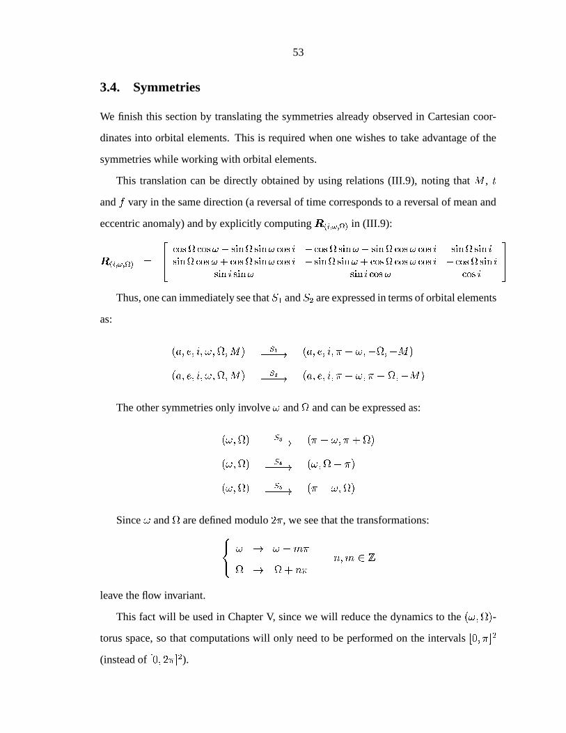
53

3.4. Symmetries

We finish this section by translating the symmetries already observed in Cartesian coor-

dinates into orbital elements. This is required when one wishes to take advantage of the

symmetries while working with orbital elements.

This translation can be directly obtained by using relations (III.9), noting that , and vary in the same direction (a reversal of time corresponds to a reversal of mean and

eccentric anomaly) and by explicitly computing in (III.9):

Thus, one can immediately see that and are expressed in terms of orbital elements

as:

The other symmetries only involve and

and can be expressed as:

# #

#

Since and

are defined modulo , we see that the transformations: #

#

leave the flow invariant.

This fact will be used in Chapter V, since we will reduce the dynamics to the -torus space, so that computations will only need to be performed on the intervals

(instead of ).

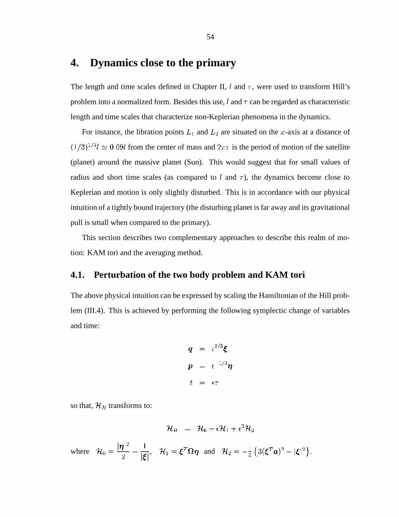
54

4. Dynamics close to the primary

The length and time scales defined in Chapter II, and , were used to transform Hill’s

problem into a normalized form. Besides this use, and can be regarded as characteristic

length and time scales that characterize non-Keplerian phenomena in the dynamics.

For instance, the libration points and are situated on the -axis at a distance of

from the center of mass and is the period of motion of the satellite

(planet) around the massive planet (Sun). This would suggest that for small values of

radius and short time scales (as compared to and ), the dynamics become close to

Keplerian and motion is only slightly disturbed. This is in accordance with our physical

intuition of a tightly bound trajectory (the disturbing planet is far away and its gravitational

pull is small when compared to the primary).

This section describes two complementary approaches to describe this realm of mo-

tion: KAM tori and the averaging method.

4.1. Perturbation of the two body problem and KAM tori

The above physical intuition can be expressed by scaling the Hamiltonian of the Hill prob-

lem (III.4). This is achieved by performing the following symplectic change of variables

and time:

so that,

transforms to:

" # # where

"

, and

.

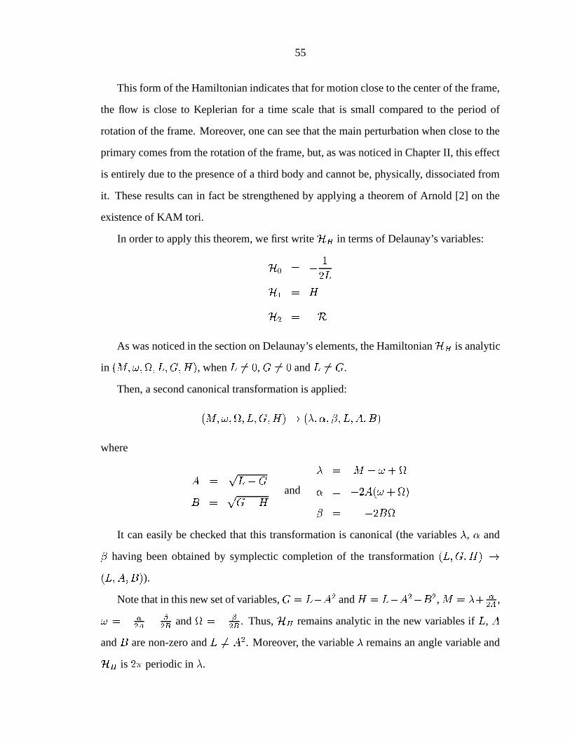
55

This form of the Hamiltonian indicates that for motion close to the center of the frame,

the flow is close to Keplerian for a time scale that is small compared to the period of

rotation of the frame. Moreover, one can see that the main perturbation when close to the

primary comes from the rotation of the frame, but, as was noticed in Chapter II, this effect

is entirely due to the presence of a third body and cannot be, physically, dissociated from

it. These results can in fact be strengthened by applying a theorem of Arnold [2] on the

existence of KAM tori.

In order to apply this theorem, we first write

in terms of Delaunay’s variables:

"

As was noticed in the section on Delaunay’s elements, the Hamiltonian

is analytic

in , when , and .

Then, a second canonical transformation is applied:

where

and

# #

#

It can easily be checked that this transformation is canonical (the variables

, and

having been obtained by symplectic completion of the transformation ).

Note that in this new set of variables, and , # ,

and

. Thus,

remains analytic in the new variables if ,

and are non-zero and . Moreover, the variable

remains an angle variable and

is periodic in

.

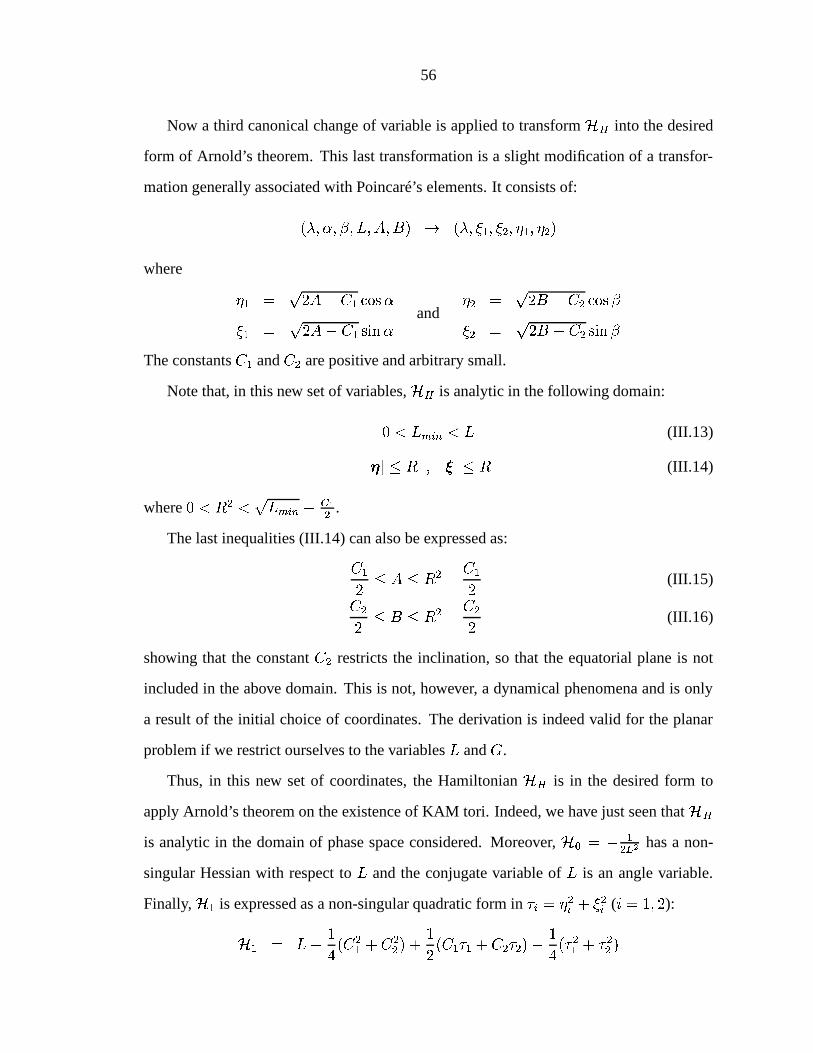
56

Now a third canonical change of variable is applied to transform

into the desired

form of Arnold’s theorem. This last transformation is a slight modification of a transfor-

mation generally associated with Poincaré’s elements. It consists of:

!

where

and

The constants and are positive and arbitrary small.

Note that, in this new set of variables,

is analytic in the following domain:

(III.13)

(III.14)

where

.

The last inequalities (III.14) can also be expressed as:

(III.15)

(III.16)

showing that the constant restricts the inclination, so that the equatorial plane is not

included in the above domain. This is not, however, a dynamical phenomena and is only

a result of the initial choice of coordinates. The derivation is indeed valid for the planar

problem if we restrict ourselves to the variables and .

Thus, in this new set of coordinates, the Hamiltonian

is in the desired form to

apply Arnold’s theorem on the existence of KAM tori. Indeed, we have just seen that

is analytic in the domain of phase space considered. Moreover, " has a non-

singular Hessian with respect to and the conjugate variable of is an angle variable.

Finally, is expressed as a non-singular quadratic form in # ( ):

# #

#

#

57

Thus, in the domain defined by inequalities (III.13)-(III.14), we have an invariant set

foliated by invariant tori on which the flow is conditionally periodic. The complement of

this set in the domain of phase space considered has very small measure (depending on

the constants chosen) but form a dense set in the domain considered.

The invariant tori correspond to small perturbation of the motion on Keplerian orbits in

a rotating frame. Thus, on these tori, the motion of a spacecraft can be well approximated

by the nearby Keplerian motion. This motion corresponds to a linear increase in the mean

anomaly and a constant rate of precession for the longitude of the ascending node.

This theorem does not give us, however, a bound on how far these results can be

applied. Indeed, the existence of these tori depends on the constants in the above variables,

and notably on the first symplectic scaling used. In particular, the region of phase space for

which the KAM tori may exist may be well below the physical surface of the primary. In

the planar case, this happens for example, as soon as the periapsis of the stable or unstable

manifold associated with the libration points is below the surface [36].

The result obtained is, however, interesting since it shows some relations between the

semi-major axis, the eccentricity and the inclination that affect the stability of the motion.

Indeed, from the inequalities (III.15), (III.16) and the definition of

and , we can see

that:

The larger the semi-major axis, the smaller the eccentricity. That is, stable, highly

elliptic motion is destroyed more rapidly than circular motion as we move away

from the center of the frame.

The higher the inclination, the smaller the angular momentum. That is, circular

orbits with given radius are more stable for low inclinations rather that for high

inclinations, thus indicating the possible destabilizing effect of high inclinations.

Finally, we should note that the existence of KAM tori does not prove the stability

of motion in the spatial problem (existence of Arnol’d diffusion), but it does prove the

stability of motion for the planar problem in the region of phase space close to the origin.

58

4.2. Averaging

While the above discussion is rigorous, it does not provide us any idea on how far from the

primary we can consider circular motion to be close to Keplerian . Perturbation methods,

while non-rigorous, give us such an estimate. This subsection briefly reviews the results

obtained in [32].

When the mean motion of the spacecraft is large compared to the mean motion of

the primary around the disturbing body, one can average over the mean anomaly of the

spacecraft to obtain the secular variation of the elements describing its motion. Moreover,

when one wants to consider time scales large compared to the period of revolution of

the primary around the disturbing body, one can average the disturbing function of the

previous averaging over the mean motion of the primary. The resulting disturbing function,

given by

"

"

is independent of time and the Lagrange planetary equations for this disturbing function

yield the secular variations of the orbital elements (except ) as a function of time, i.e.,

the variations that occur on a time scale much larger than .

The result of this double averaging are a zero change in semi-major axis and an inte-

grable system for , and

if we restrict ourselves to the order in eccentricity (i.e.,

orbits close to circular):

#

# #

The resulting integration indicates two distinct realms of motion depending on the initial

inclination.

While the theorem uses averaging on , the resulting small parameter given by the theorem is justguaranteed to exist, but no bound is given on its magnitude. We used an existence theorem.

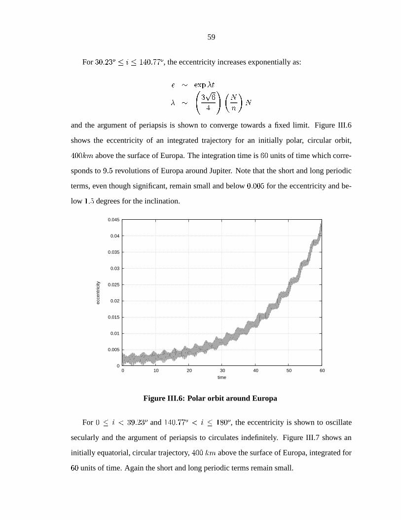
59

For ! ! , the eccentricity increases exponentially as:

"

and the argument of periapsis is shown to converge towards a fixed limit. Figure III.6

shows the eccentricity of an integrated trajectory for an initially polar, circular orbit, above the surface of Europa. The integration time is units of time which corre-

sponds to revolutions of Europa around Jupiter. Note that the short and long periodic

terms, even though significant, remain small and below for the eccentricity and be-

low degrees for the inclination.

0

0.005

0.01

0.015

0.02

0.025

0.03

0.035

0.04

0.045

0 10 20 30 40 50 60

ecce

ntric

ity

time

Figure III.6: Polar orbit around Europa

For ! and ! ! , the eccentricity is shown to oscillate

secularly and the argument of periapsis to circulates indefinitely. Figure III.7 shows an

initially equatorial, circular trajectory, above the surface of Europa, integrated for

units of time. Again the short and long periodic terms remain small.

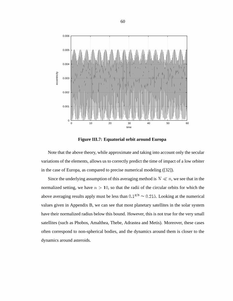
60

0

0.001

0.002

0.003

0.004

0.005

0.006

0 10 20 30 40 50 60

ecce

ntric

ity

time

Figure III.7: Equatorial orbit around Europa

Note that the above theory, while approximate and taking into account only the secular

variations of the elements, allows us to correctly predict the time of impact of a low orbiter

in the case of Europa, as compared to precise numerical modeling ([32]).

Since the underlying assumption of this averaging method is , we see that in the

normalized setting, we have , so that the radii of the circular orbits for which the

above averaging results apply must be less than . Looking at the numerical

values given in Appendix B, we can see that most planetary satellites in the solar system

have their normalized radius below this bound. However, this is not true for the very small

satellites (such as Phobos, Amalthea, Thebe, Adrastea and Metis). Moreover, these cases

often correspond to non-spherical bodies, and the dynamics around them is closer to the

dynamics around asteroids.

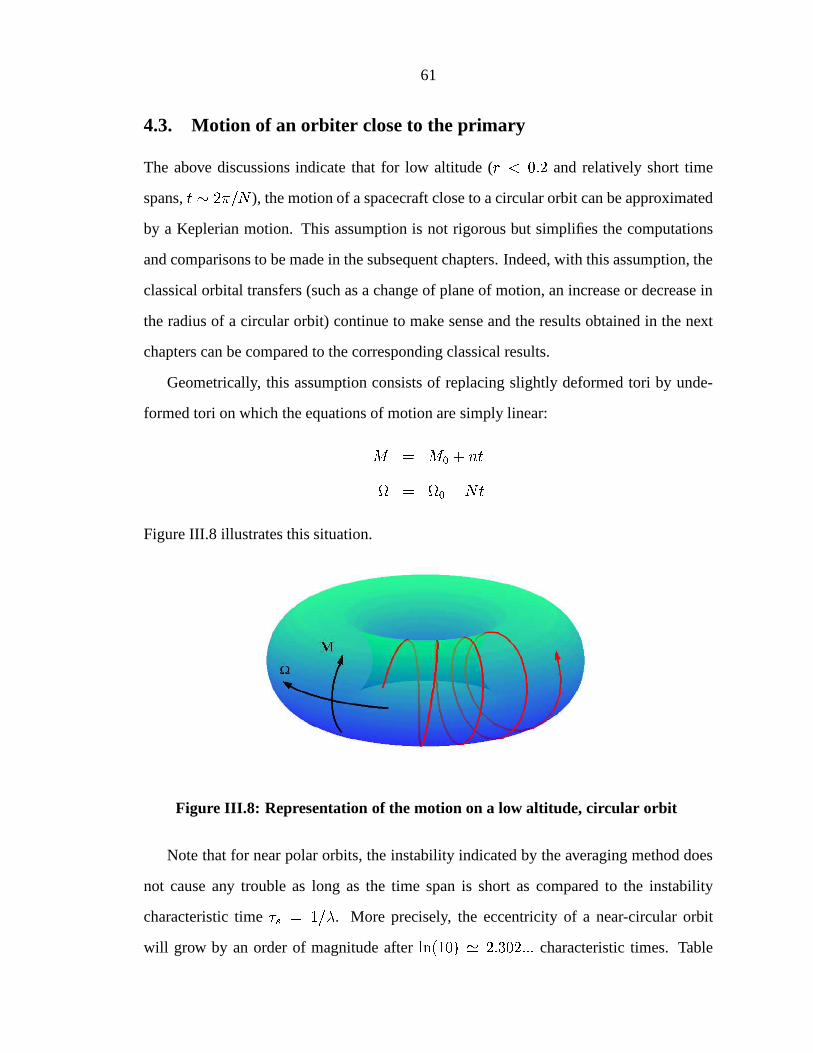
61

4.3. Motion of an orbiter close to the primary

The above discussions indicate that for low altitude ( and relatively short time

spans, ), the motion of a spacecraft close to a circular orbit can be approximated

by a Keplerian motion. This assumption is not rigorous but simplifies the computations

and comparisons to be made in the subsequent chapters. Indeed, with this assumption, the

classical orbital transfers (such as a change of plane of motion, an increase or decrease in

the radius of a circular orbit) continue to make sense and the results obtained in the next

chapters can be compared to the corresponding classical results.

Geometrically, this assumption consists of replacing slightly deformed tori by unde-

formed tori on which the equations of motion are simply linear:

" # "

Figure III.8 illustrates this situation.

Figure III.8: Representation of the motion on a low altitude, circular orbit

Note that for near polar orbits, the instability indicated by the averaging method does

not cause any trouble as long as the time span is short as compared to the instability

characteristic time . More precisely, the eccentricity of a near-circular orbit

will grow by an order of magnitude after characteristic times. Table

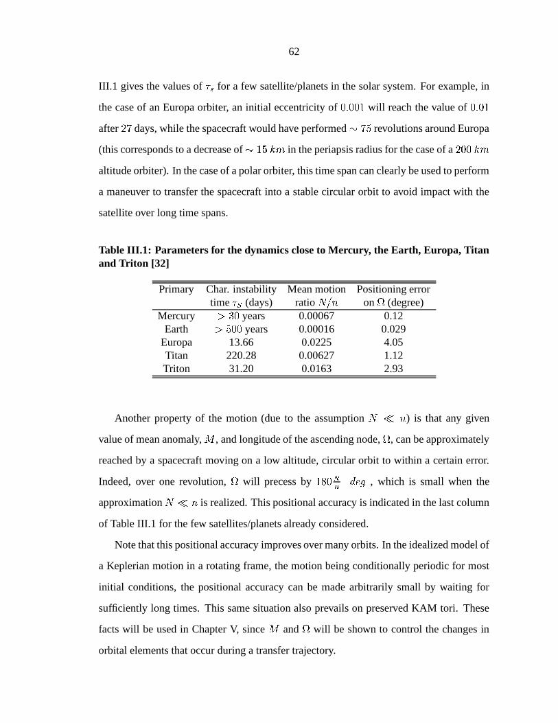
62

III.1 gives the values of for a few satellite/planets in the solar system. For example, in

the case of an Europa orbiter, an initial eccentricity of will reach the value of

after days, while the spacecraft would have performed revolutions around Europa

(this corresponds to a decrease of

in the periapsis radius for the case of a

altitude orbiter). In the case of a polar orbiter, this time span can clearly be used to perform

a maneuver to transfer the spacecraft into a stable circular orbit to avoid impact with the

satellite over long time spans.

Table III.1: Parameters for the dynamics close to Mercury, the Earth, Europa, Titanand Triton [32]

Primary Char. instability Mean motion Positioning errortime (days) ratio on

(degree)

Mercury years 0.00067 0.12Earth years 0.00016 0.029

Europa 13.66 0.0225 4.05Titan 220.28 0.00627 1.12Triton 31.20 0.0163 2.93

Another property of the motion (due to the assumption ) is that any given

value of mean anomaly, , and longitude of the ascending node,

, can be approximately

reached by a spacecraft moving on a low altitude, circular orbit to within a certain error.

Indeed, over one revolution,

will precess by , which is small when the

approximation is realized. This positional accuracy is indicated in the last column

of Table III.1 for the few satellites/planets already considered.

Note that this positional accuracy improves over many orbits. In the idealized model of

a Keplerian motion in a rotating frame, the motion being conditionally periodic for most

initial conditions, the positional accuracy can be made arbitrarily small by waiting for

sufficiently long times. This same situation also prevails on preserved KAM tori. These

facts will be used in Chapter V, since and

will be shown to control the changes in

orbital elements that occur during a transfer trajectory.

63

Finally, we should note that the assumption made on the motion of a low altitude,

circular orbit can be overcome by computing, for example, the short periodic variations

of the elements

, thus including the slight deformation of the tori into the picture. As

long as these perturbations remain small, the large fuel savings obtained in the subsequent

applications would only be slightly changed, but the possibility of performing them would,

of course, not be changed.

5. Dynamics far from the primary

This section investigates the asymptotic form of the motion of a particle when far form

the primary. This situation would occur, for example, after a particle escapes from the

vicinity of the primary through a throat formed by the zero velocity surfaces when .

Also, in the case of an orbiter (i.e., in the framework of the restricted Hill problem), these

asymptotic dynamics allow us to patch any escaping solution of the Hill problem onto an

outer solution, corresponding to a two body motion around the disturbing body, to obtain

an approximate solution of the restricted three body problem.

5.1. Equations of motion

Motion far from the primary can be obtained by scaling the Hamiltonian of the Hill’s

problem using the following symplectic change of variable:

Under this transformation,

is rewritten as:

(III.17)

or by direct numerical integration of the low altitude, initial orbits.

64

That is:

# where

has the same expression as in Chapter II (the only difference being in the unit

chosen):

Thus, when looking at motion far from the primary, the Hill’s equations of motion

reduce to the linearized motion about the circular orbit defined by the motion of the pri-

mary around the disturbing body. This is again the Clohessy-Wiltshire equations.

Note that this fact is physically reasonable since the Hill problem has been defined

as describing the relative motion of two small masses whose center of mass follows an

approximately circular orbit around a massive body. When the small masses are far from

each other, their gravitational attraction is negligible and the particle are thus only moving

under the influence of the massive body on a nearly circular orbit.

Note also that because of the scaling, “infinitely far” in Hill’s coordinates only corre-

sponds to a relatively small displacement when looking at the order of length scale deter-

mined by the large disturbing body.

From (III.17), we immediately compute the equations of motion:

# #

or, expressed in components:

#

#

or the center of mass of the two small masses.

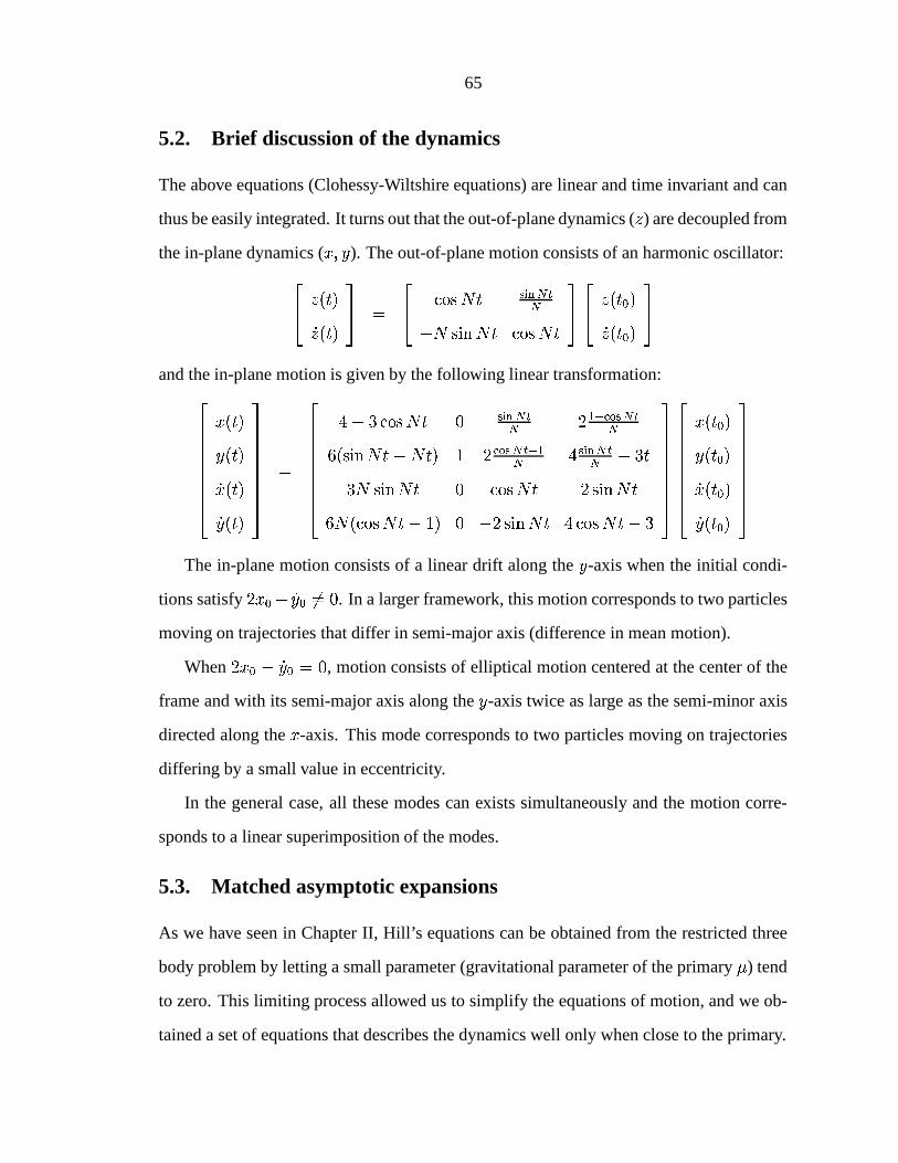
65

5.2. Brief discussion of the dynamics

The above equations (Clohessy-Wiltshire equations) are linear and time invariant and can

thus be easily integrated. It turns out that the out-of-plane dynamics ( ) are decoupled from

the in-plane dynamics ( ). The out-of-plane motion consists of an harmonic oscillator:

" "

and the in-plane motion is given by the following linear transformation:

" " " "

The in-plane motion consists of a linear drift along the -axis when the initial condi-

tions satisfy " " . In a larger framework, this motion corresponds to two particles

moving on trajectories that differ in semi-major axis (difference in mean motion).

When " " , motion consists of elliptical motion centered at the center of the

frame and with its semi-major axis along the -axis twice as large as the semi-minor axis

directed along the -axis. This mode corresponds to two particles moving on trajectories

differing by a small value in eccentricity.

In the general case, all these modes can exists simultaneously and the motion corre-

sponds to a linear superimposition of the modes.

5.3. Matched asymptotic expansions

As we have seen in Chapter II, Hill’s equations can be obtained from the restricted three

body problem by letting a small parameter (gravitational parameter of the primary ) tend

to zero. This limiting process allowed us to simplify the equations of motion, and we ob-

tained a set of equations that describes the dynamics well only when close to the primary.

66

Note also that, when performing this procedure, a simultaneous scaling that depends

on this small parameter was also applied so that when , the length scale also tends

to zero. Equivalently, when looking at the dynamics from the point of view of the Hill’s

length scale, we let the length scale and the gravitational parameter of the disturbing,

massive body tend to infinity.

Now, in the above derivation of the Clohessy-Wiltshire equations, we applied this in-

verse scaling (length scale goes to infinity) on the Hill problem. That is, overall we per-

formed two opposite limiting processes, and one can wonder what happens if the order

of the limits is reversed. As we will see below, this procedure leads to the same set of

equations, the Clohessy-Wiltshire equations.

The procedure just outlined is typical of singularly perturbed problems where an ap-

proximate solution is constructed by matching two asymptotic solutions. Singularly per-

turbed problems generally consist of a set of differential equations depending on a small

parameter in such a way that either the equations degenerate when the small parameter is

set to zero or the small parameter multiplies a singularity of the equations. For example,

this would occur if the highest derivative (either spatial or temporal) of the equations is

multiplied by the small parameter:

# # or

as happens in fluids mechanics when the Reynolds number,

, is large.

In our case, the small parameter multiplies a singularity of the equations correspond-

ing to the center of the primary. Recall from Chapter II that the restricted problem, as

formulated in the body centered frame and normalized, is expressed as:

# # (III.18)

If the small parameter is set to zero in the above equations, the equations simplify (with

much information lost) to the point that all the boundary conditions of the problem cannot

be satisfied: the no-slip condition cannot be satisfied in fluid mechanics and, in our case,

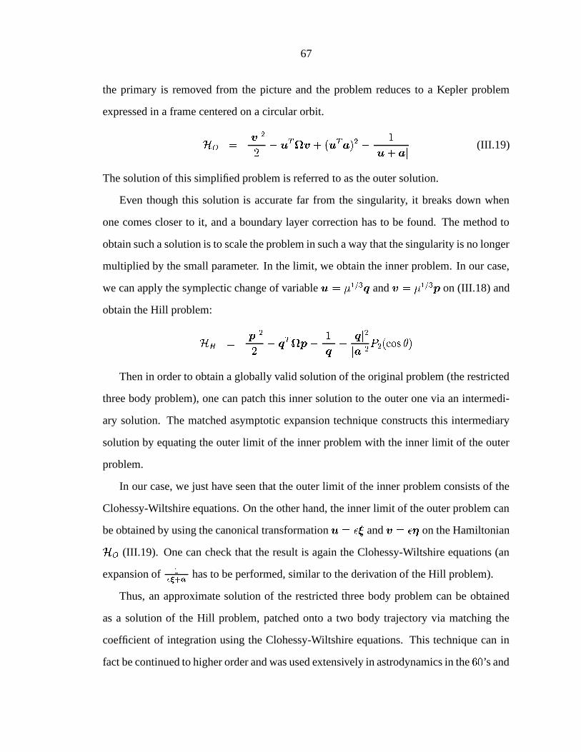
67

the primary is removed from the picture and the problem reduces to a Kepler problem

expressed in a frame centered on a circular orbit.

# # (III.19)

The solution of this simplified problem is referred to as the outer solution.

Even though this solution is accurate far from the singularity, it breaks down when

one comes closer to it, and a boundary layer correction has to be found. The method to

obtain such a solution is to scale the problem in such a way that the singularity is no longer

multiplied by the small parameter. In the limit, we obtain the inner problem. In our case,

we can apply the symplectic change of variable and on (III.18) and

obtain the Hill problem:

#

Then in order to obtain a globally valid solution of the original problem (the restricted

three body problem), one can patch this inner solution to the outer one via an intermedi-

ary solution. The matched asymptotic expansion technique constructs this intermediary

solution by equating the outer limit of the inner problem with the inner limit of the outer

problem.

In our case, we just have seen that the outer limit of the inner problem consists of the

Clohessy-Wiltshire equations. On the other hand, the inner limit of the outer problem can

be obtained by using the canonical transformation and on the Hamiltonian

(III.19). One can check that the result is again the Clohessy-Wiltshire equations (an

expansion of has to be performed, similar to the derivation of the Hill problem).

Thus, an approximate solution of the restricted three body problem can be obtained

as a solution of the Hill problem, patched onto a two body trajectory via matching the

coefficient of integration using the Clohessy-Wiltshire equations. This technique can in

fact be continued to higher order and was used extensively in astrodynamics in the ’s and

68

’s, when interplanetary trajectories were analyzed using patched conic approximations

[5].

In our case, this shows that the escaping solutions to be obtained in chapter VI can

be embedded into a more global framework (for the case of an orbiter) to analyze, for

example, possible future impacts of the spacecraft with the primary (after one or multiple

loops around the disturbing body). Matching between the regions near the libration points

and infinity can also be performed by using series expansions, as given in a paper by Hénon

and Petit [15].

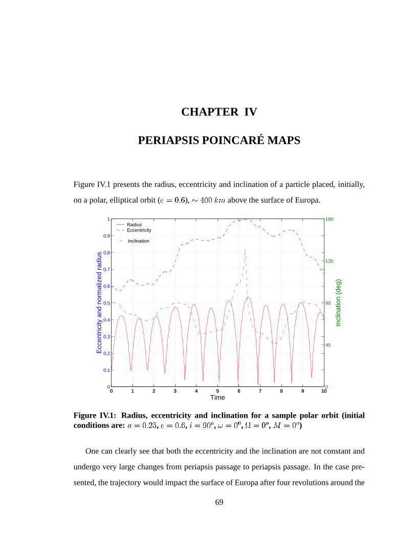
CHAPTER IV

PERIAPSIS POINCARÉ MAPS

Figure IV.1 presents the radius, eccentricity and inclination of a particle placed, initially,

on a polar, elliptical orbit ( ),

above the surface of Europa.

0 1 2 3 4 5 6 7 8 9 100

0.1

0.2

0.3

0.4

0.5

0.6

0.7

0.8

0.9

1

Time

Ecc

entr

icity

and

nor

mal

ized

rad

ius

RadiusEccentricity

0 1 2 3 4 5 6 7 8 9 100

45

90

135

180

Incl

inat

ion

(deg

)

Inclination

Figure IV.1: Radius, eccentricity and inclination for a sample polar orbit (initialconditions are: , , ! ,

", ! , ! )

One can clearly see that both the eccentricity and the inclination are not constant and

undergo very large changes from periapsis passage to periapsis passage. In the case pre-

sented, the trajectory would impact the surface of Europa after four revolutions around the

69

70

planetary satellite.

The aim of the chapter is to present a systematic way of analyzing these dynamics by

considering them from periapsis passage to periapsis passage. Even though these periapsis

maps can be computed numerically, estimates of the functional form of these maps may

be preferable to obtain a global qualitative picture of these dynamics. An attempt to obtain

such estimates is presented in this chapter via the use of Picard’s method of successive

approximations [41].

The first section defines the periapsis maps as Poincaré maps between surfaces of sec-

tion defined by the periapsis condition. It is shown in particular that these maps are well

defined (transversal to the flow) over an interesting range of initial conditions and they

allow us to partition the position space into periapsis or apoapsis exclusive regions.

Section 2 reviews the process of Picard’s method of successive approximations and

investigates their use for the integration of Hamiltonian systems. It is shown in particular

that each step of the process defines a symplectic map for a restricted class of Hamilto-

nian systems (which includes integrable problems) and a reduction process can be used to

transform the process into an energy preserving one.

In section 3, the first step of the method is applied to the system of differential equa-

tions defining the Hill’s problem, resulting in approximate expressions for the changes

in energy and angular momentum over one orbit. A numerical check on the accuracy of

these expressions is given, showing the validity to within for a large range of initial

conditions.

Finally, section 4 gives some qualitative results derived from the previous approximate

expressions. Notably, the dependence on the initial conditions of the changes of the orbital

elements over one orbit are discussed.

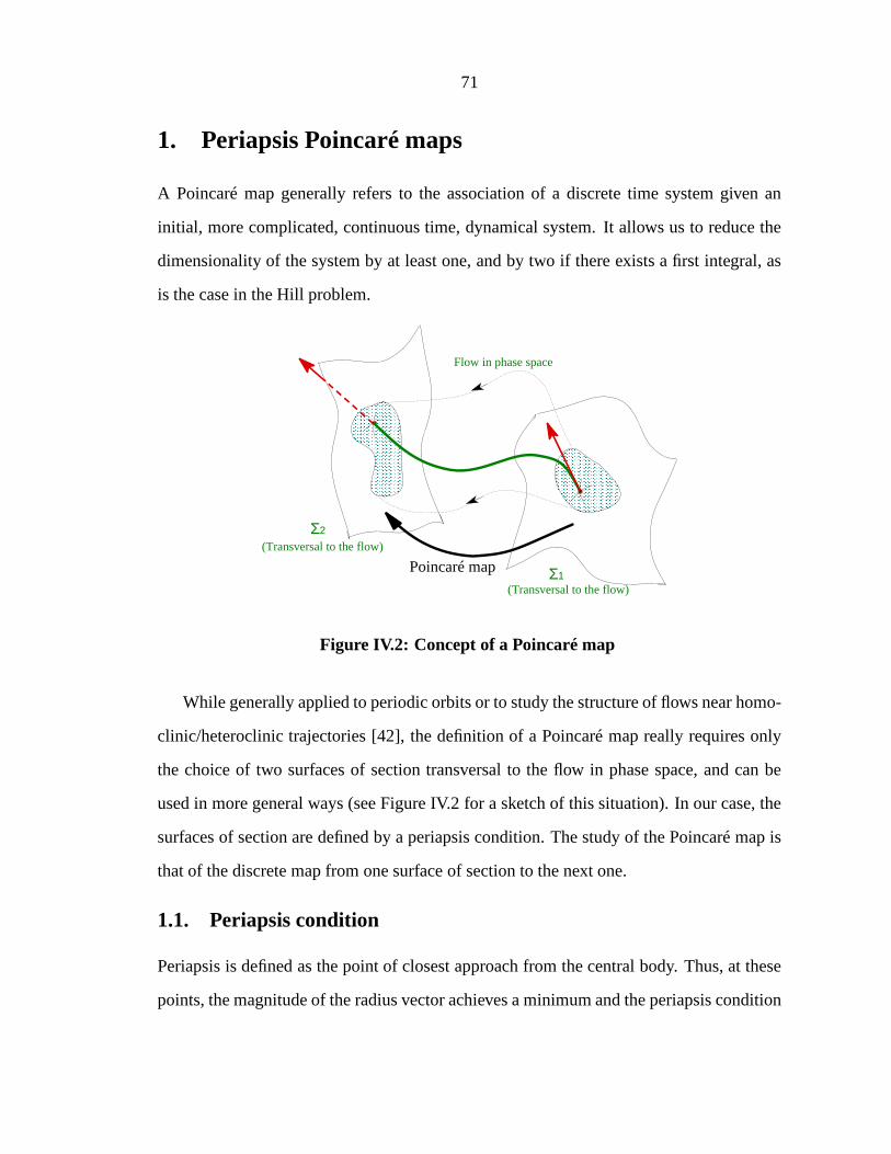
71

1. Periapsis Poincaré maps

A Poincaré map generally refers to the association of a discrete time system given an

initial, more complicated, continuous time, dynamical system. It allows us to reduce the

dimensionality of the system by at least one, and by two if there exists a first integral, as

is the case in the Hill problem.

Σ2

Σ1

Flow in phase space

Poincaré map(Transversal to the flow)

(Transversal to the flow)

Figure IV.2: Concept of a Poincaré map

While generally applied to periodic orbits or to study the structure of flows near homo-

clinic/heteroclinic trajectories [42], the definition of a Poincaré map really requires only

the choice of two surfaces of section transversal to the flow in phase space, and can be

used in more general ways (see Figure IV.2 for a sketch of this situation). In our case, the

surfaces of section are defined by a periapsis condition. The study of the Poincaré map is

that of the discrete map from one surface of section to the next one.

1.1. Periapsis condition

Periapsis is defined as the point of closest approach from the central body. Thus, at these

points, the magnitude of the radius vector achieves a minimum and the periapsis condition

72

can be formulated as :

(IV.1)

Expressed in terms of the position and velocity vectors, this definition is equivalent to:

#

(IV.2)

where represents the acceleration of the particle in the rotating frame.

Thus we can see that periapsis is defined by a geometrical condition ( orthogonal to ) plus a condition on the speed of the particle. In fact, the geometrical condition (apsis

condition) projects onto the whole Hill region,

, while the restriction imposed by the

periapsis condition is more restrictive, as we will see in the next subsection. Note that

when #

, the magnitude of the radius vector achieves a maximum. At such

points, the particle is said to be at apoapsis.

Note that, even though and

are dependent on the frame, it can be easily checked

that the notion of periapsis (or apoapsis) is independent of the frame. That is: # # (IV.3)

where the subscripts and refer, respectively, to an inertial and a rotating frame centered

at the center of mass of the attracting body.

The notion of periapsis (or apoapsis) does depend, however, on the force field consid-

ered. For example, the notion as defined in the Hill problem and the Kepler problem are

not equivalent.

For the Kepler problem in a rotating frame, we have ,

so that periapsis is achieved when and are orthogonal and

.

Strictly speaking, one can also have $ at periapsis but we will restrict ourselves to the definition

given.

73

The acceleration in the Hill problem differs from that of the Kepler problem in a rotat-

ing frame by the term # . That is the periapsis condition is given by:

# (IV.4)

Thus, for , a particle can be at periapsis in the Hill problem while

being at apoapsis in the Kepler problem. For , the situation is opposite,

that is, a particle can be at apoapsis in the Hill problem while being at periapsis in the

Kepler problem. Note that these cases can occur only for small eccentricities, i.e., nearly

circular orbits.

Finally, one can notice that the notion of periapsis and apoapsis agree in both problems

when , which corresponds to a cone in position space with apex at the

origin, axis given by the -axis and with normal section corresponding to circles in the

coordinates. The first situation ( ) occurs “outside” the cone while

the other case (

) occurs “inside” the cone (i.e., the region containing

the axis).

In the remainder, our focus will be on the case of the Hill problem and periapsis will

thus be defined by (IV.4).

1.2. First consequences

An interesting fact in the Hill problem (this also holds for the restricted three body prob-

lem) is that the periapsis condition (resp. apoapsis condition) reduces to a condition in-

dependent of the velocity in the planar case. Indeed, one can use the Jacobi constant

to express the speed of the particle in terms of its position and

energy.

More precisely, in the planar case, at any apsis in the direct case,

while at any apsis in the retrograde case. Table IV.1 summarizes the

implications of this formulation.

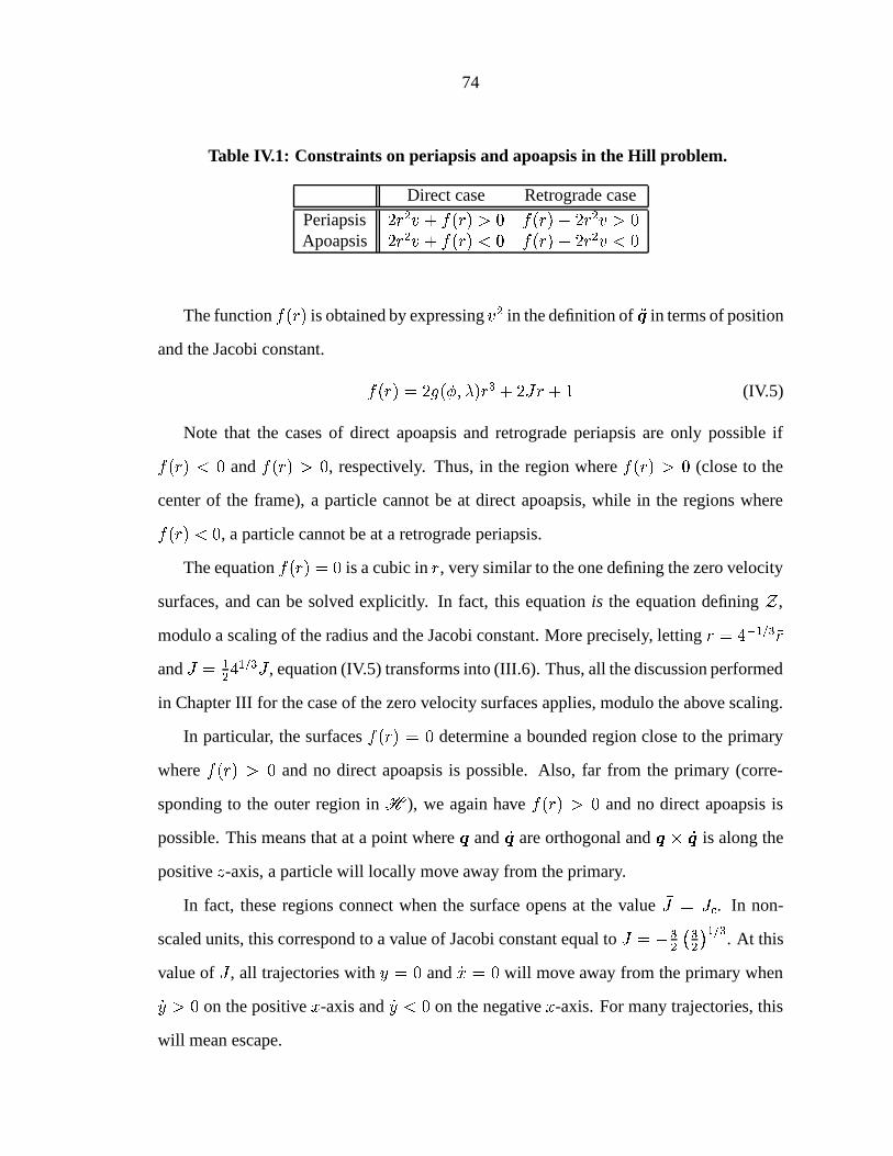
74

Table IV.1: Constraints on periapsis and apoapsis in the Hill problem.

Direct case Retrograde case

Periapsis # Apoapsis #

The function is obtained by expressing in the definition of

in terms of position

and the Jacobi constant.

# ! # (IV.5)

Note that the cases of direct apoapsis and retrograde periapsis are only possible if

and , respectively. Thus, in the region where (close to the

center of the frame), a particle cannot be at direct apoapsis, while in the regions where

, a particle cannot be at a retrograde periapsis.

The equation is a cubic in , very similar to the one defining the zero velocity

surfaces, and can be solved explicitly. In fact, this equation is the equation defining ,

modulo a scaling of the radius and the Jacobi constant. More precisely, letting and

, equation (IV.5) transforms into (III.6). Thus, all the discussion performed

in Chapter III for the case of the zero velocity surfaces applies, modulo the above scaling.

In particular, the surfaces determine a bounded region close to the primary

where and no direct apoapsis is possible. Also, far from the primary (corre-

sponding to the outer region in

), we again have and no direct apoapsis is

possible. This means that at a point where and are orthogonal and is along the

positive -axis, a particle will locally move away from the primary.

In fact, these regions connect when the surface opens at the value . In non-

scaled units, this correspond to a value of Jacobi constant equal to

. At this

value of , all trajectories with and will move away from the primary when

on the positive -axis and

on the negative -axis. For many trajectories, this

will mean escape.

75

Similarly, outside the region , the motion is constrained so that no retrograde

periapsis is possible. It can be easily proven that such regions always exist for . In

fact, all points on corresponds to such a situation when . Recall that this value

of correspond to the tangency of with the radial lines when and lies in the

region of forbidden motion for . Thus, for , all points on in the inner

region corresponds to apoapsis, while all points of in the outer region correspond to

periapsis. When , the situation holds equally well, if the inner region is determined

by . In fact, this result shows that the outer component of meet at

and thus crosses the -axis at when .

Finally, we should note that when , the inner component of lies about

midway between the origin and and exactly midway on the -axis, i.e., at .

Figures IV.3 illustrates these situations in the quadrant of the plane (the other

quadrants being obtained by symmetries).

The above discussion can, in fact, be strengthened by looking at the signs (and hence

the roots) of the functions and # , where is expressed in terms of

position and the Jacobi constant. These functions involve square roots and the zeros cannot

be solved explicitly. These zeros can, however, be easily computed numerically. In fact,

these zeros are the roots of the degree polynomial # :

# ! # # ! # (IV.6)

The roots of can be sorted according to the sign of so as to make them

correspond to the zeros of the above functions. Therefore, with the help of Table IV.1, one

obtains the following diagram for the partioning of a radial line (assuming the roots exist)

between periapsis and apoapsis regions:

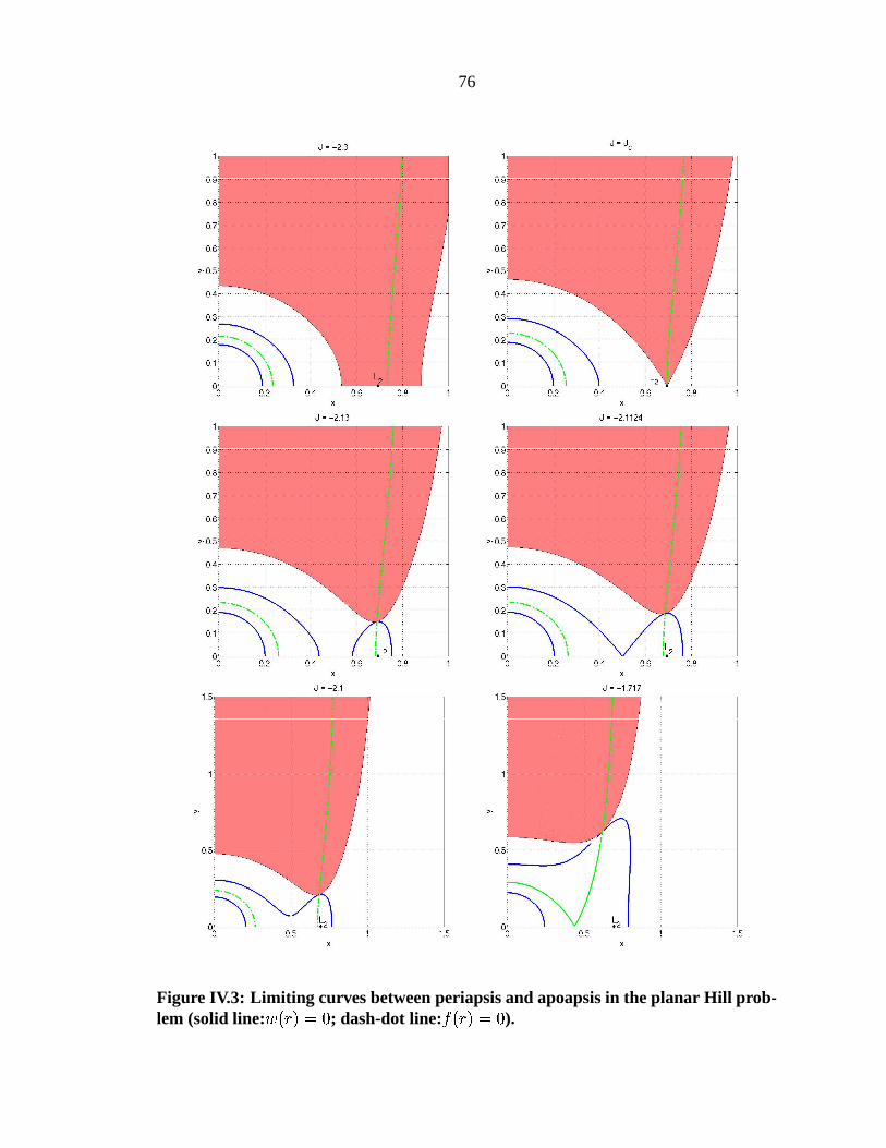
76

Figure IV.3: Limiting curves between periapsis and apoapsis in the planar Hill prob-lem (solid line: ; dash-dot line: ).

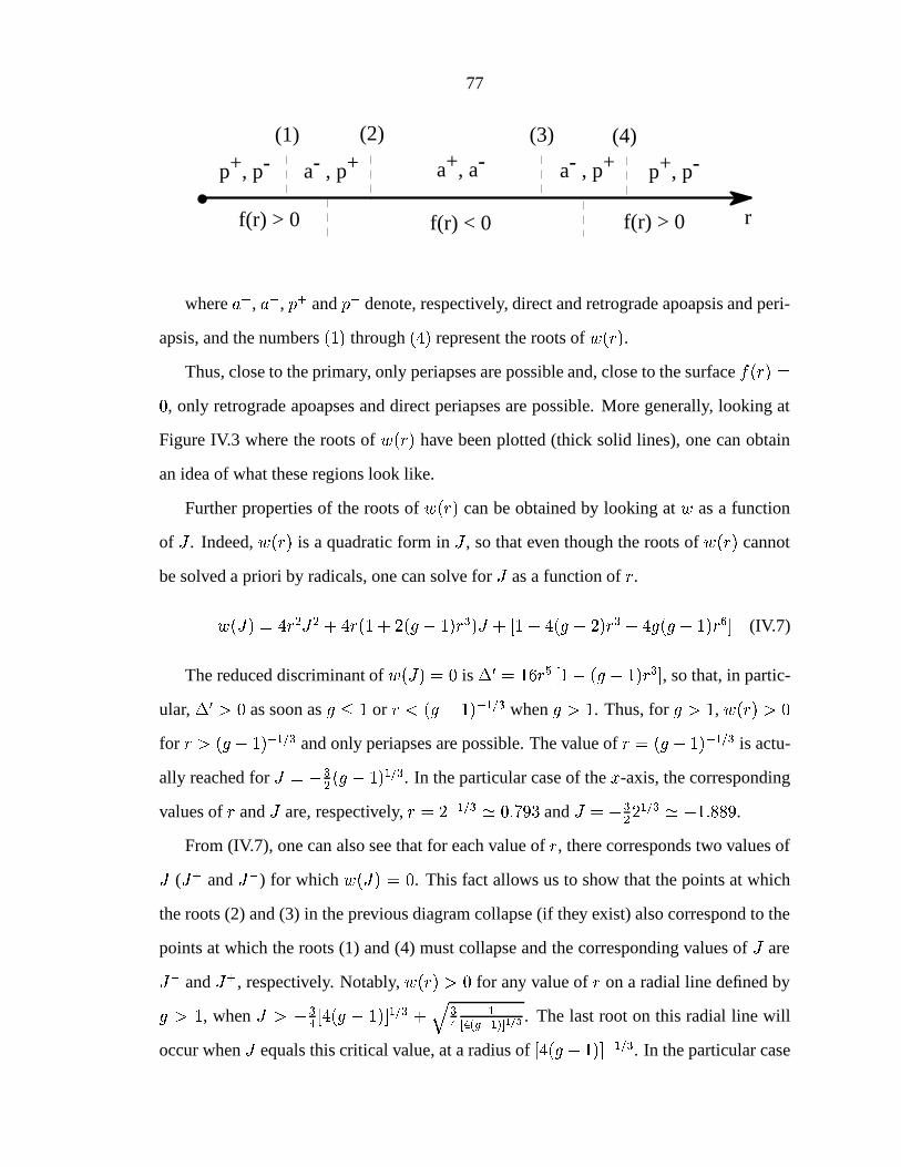
77

f(r) > 0 f(r) < 0 f(r) > 0

p+, p- a- , p+ a+, a- a- , p+ p+, p-

r

(1) (2) (3) (4)

where , ,

and denote, respectively, direct and retrograde apoapsis and peri-

apsis, and the numbers through represent the roots of .Thus, close to the primary, only periapses are possible and, close to the surface

, only retrograde apoapses and direct periapses are possible. More generally, looking at

Figure IV.3 where the roots of have been plotted (thick solid lines), one can obtain

an idea of what these regions look like.

Further properties of the roots of can be obtained by looking at as a function

of . Indeed, is a quadratic form in , so that even though the roots of cannot

be solved a priori by radicals, one can solve for as a function of .

# # # # # (IV.7)

The reduced discriminant of is , so that, in partic-

ular, as soon as or when . Thus, for ,

for and only periapses are possible. The value of is actu-

ally reached for . In the particular case of the -axis, the corresponding

values of and are, respectively, and .

From (IV.7), one can also see that for each value of , there corresponds two values of

(

and ) for which . This fact allows us to show that the points at which

the roots (2) and (3) in the previous diagram collapse (if they exist) also correspond to the

points at which the roots (1) and (4) must collapse and the corresponding values of are

and

, respectively. Notably, for any value of on a radial line defined by

, when #

. The last root on this radial line will

occur when equals this critical value, at a radius of . In the particular case

78

of the -axis, these critical values of collapse and disappearance of roots are " and

and , respectively. This is in

concordance with the plots shown on Figure IV.3.

Another interesting consequence of these results is that for low values of the Jacobi

constant, the two inner roots of lie on curves which are close to circular and the

Hill’s periodic orbits which are almost circular must, per force, lie close to these curves.

Indeed, the periapsis of such an orbit must lie below the first curve in the direct case and

its apoapsis must lie above it. Since the eccentricity is small at each point of these orbits,

the two apses must be close together. The same situation holds true in the retrograde case

with the curve. In fact, the situation is more general and remains true for any quasi-

periodic, quasi-circular orbits. That is, the KAM tori corresponding to trajectories with

small eccentricity in the rotating Kepler problem must lie close to these curves, when they

exist, giving us a qualitative idea of their evolution as a function of .

Finally, we should note that in the spatial problem, where represents the inclination as defined in the rotating frame. The above results apply to this

case by replacing the direct and retrograde cases with below or above ! . The limits

between regions with only periapsis or apoapsis possible are independent of and are thus

given by the roots of .

1.3. Transversality

As was noted in the introduction of the present section, Poincaré maps are defined by

choosing some surface of section transversal to the flow. Transversality means that the flow

generated by the differential equations under consideration crosses, locally, the surfaces of

section from one side to the other. This requirement of transversality is indeed needed to

avoid degeneracies, such as circular orbits in the Kepler problem for a periapsis Poincaré

map.

In our case, the flow is generated by the vector field where is given

79

by Hill equations:

# (IV.8)

The surfaces of section are first defined by the apsis condition, , so that the

transversality condition requires that . That is:

# (IV.9)

Thus, in the case of a periapsis Poincaré map, transversality is automatically satisfied

(with the definition we adopted). In fact, the same holds true for an apoapsis Poincaré map

and one can define periapsis to apoapsis maps, as well.

Note that the cases where are exactly given by the roots of , as

discussed in the previous subsection. Away from these roots, periapsis and apoapsis are

well defined.

By looking at the dynamics via Poincaré maps, the dimensionality of the initial system

is reduced by one. Moreover, one can also restrict the map to lie in a given energy manifold

to remove one additional dimension. Thus, in the spatial Hill problem , we obtain-

dimensional maps, while in the planar problem, one obtains a -dimensional map. As we

have seen in the previous subsection, these maps can be parameterized by the position

and the inclination in the rotating frame. The position can either be defined via Cartesian

coordinates or by using spherical coordinates.

We should note that other restrictions of the maps are possible and will be used in the

subsequent sections and chapters. Indeed, one can consider a restricted region of phase

space (as defined, for example, by some fixed value of a set of orbital elements) and look

at their image under the maps. As compared to the more classical usage of Poincaré

maps, we will study the one-time iterate of the maps to obtain numerical conditions on the

existence of certain transfers, rather than analyzing the asymptotic behavior of these maps.

In the realm of the same idea, note that the periapsis Poincaré maps, as defined above,

are not canonical (which is preferable for theoretical investigations), but can be slightly

80

changed so as to become canonical. Indeed, in the region of phase space where the notion

of periapsis between the Hill and Kepler problems agree, one can define periapsis as the

points where the mean anomaly, , is zero (modulo ). Then, a canonical map can

be obtained from Delaunay’s variables by considering the surface of section defined by

the condition and restricting the flow to the energy manifold by computing

from the expression of the Jacobi constant. A similar map can be defined with the

modified set of Delaunay’s variable (see previous chapter). Even though the numerical

applications which are presented in chapter V and VI do not use these formulations, the

next few sections implicitly rely on them.

2. Picard’s method of successive approximations

Picard’s method of successive approximations is a method that can be used to prove the

existence and uniqueness of solutions to ordinary differential equations by building a se-

quence of functions that converge uniformly towards the solution of the problem. When

applied to the case of a Poincaré map, each approximate function yields an approximation

of the Poincaré map by evaluating the functions on the surfaces of section.

This section reviews this method, emphasizing the case of Hamiltonian systems where

it is shown that each approximate function generated is symplectic for a restricted class

of Hamiltonian, and a modification of Picard’s method is also presented to yield energy

preserving maps.

2.1. General case

Consider a general system of ordinary differential equations:

(IV.10)

The existence and uniqueness of solutions satisfying the initial conditions " "

can be proven if is continuous in and Lipschitz in , uniformly in , and Picard’s

method can be used to prove this fact.

81

The method consists of considering the mapping :

" #

(IV.11)

and showing that it corresponds to a contraction mapping, so that the existence of a unique

fixed point (the solution) is guaranteed. Moreover, we know that for any initial condition

close to the fixed point, iterates of the map converge uniformly and exponentially towards

the fixed point. That is, locally, the sequence of functions:

" "

" #

"

" #

converges uniformly towards the solution of the original problem (IV.10).

More precisely, if is bounded by and is Lipschitz, with constant , in in some

region " and

" , then any function whose graph is contained

in that region will converge towards the solution of (IV.10) with initial condition " . The

error between the solution and the approximation is given by:

(IV.12)

where

represents the maximum error of " on the domain " .

Thus, assuming that the approximation has been computed, one can compute the

change in the state between " and " # , by evaluating at these instants:

" # "

(IV.13)

That is, we obtained an approximation of the time map of the flow around " .

Also, one can as well consider the time maps and obtain similar estimates.

82

2.2. Hamiltonian case

We know that Hamiltonian flows preserve the Hamiltonian function (energy) in the au-

tonomous case, as well as the symplectic structure on the underlying phase space (gener-

ally the cotangent bundle of the configuration space). That is, for each time , the map that

associates the initial state " to the state value at time is a canonical mapping. Therefore it

seems preferable in long term integrations of a Hamiltonian system to prefer either energy

preserving or symplectic preserving schemes

. Thus, in the case of Picard’s method of

successive approximations, one can ask if the contracting map is symplectic or energy

preserving.

More precisely, recall that Hamilton’s equations can be written as

where represents the -dimensional state vector and is the symplectic

matrix. Then Picard’s method of successive approximations generates the maps:

" " # (IV.14)

where is the approximate solution at the iteration of the process. Thus, the

question is to determine if is symplectic ( fixed).

First iterate map

The first step consists of checking if is symplectic. In order to see this, we only need

to compute and see if it is equal to .

One can easily compute that # " , so that:

#

(IV.15)

Thus, is symplectic if .Preserving both the energy and the symplectic structure has been shown by Z.Ge and J.Marsden to be

equivalent to exactly integrating the equations, modulo a reparameterization of time.Strictly speaking, one needs only require that !

! with $but we restrict ourselves to the non-scaling case.

83

In the autonomous case (

independent of ), the condition simplifies to:

(IV.16)

and the first step of Picard’s method corresponds to an Euler step since the map (IV.14)

reduces to " " # " " . However, higher order steps differ, in

general, from Taylor’s series expansions in a similar way as in the non-autonomous case.

We restrict ourselves to the autonomous case in this subsection for simplicity.

Expressing the above condition in terms of the conjugate variables and

, one can

easily check that it is equivalent to:

symmetric

(IV.17)

Note that in the case of an integrable system,

only depends on the action variables, and it is clear that the above conditions are satisfied.

For non-integrable systems, on can write

as an integrable part " that only de-

pends on the action variables, plus a disturbing function .

" # (IV.18)

Then, it can be easily shown that the above conditions are equivalent to :

"

" #

"

(IV.19)

These conditions are certainly restrictive, but are not restricted to only integrable

systems. For example, in the case of a perturbed Kepler problem in a rotating frame, " # in Delaunay’s variables, and any disturbing function

that only depends

on , , and

will satisfy the above conditions.

84

% iterate map

In the case of higher order approximations, it can be shown that Picard’s method leads to

symplectic maps for the class of Hamiltonian satisfying the relation:

(IV.20)

for any and in the domain under consideration.

Even though the class of Hamiltonian systems satisfying this condition includes all

autonomous integrable systems, it seems too unwieldy to be of practical interest, and in

particular the Hamiltonian of the Hill problem does not belong to that class. Instead, one

can ask if Picard’s method preserve the Hamiltonian function.

Energy preserving maps

Away from an equilibrium, , and one can locally solve for one coordinate (say )

in terms of the others.

(IV.21)

where the bar operation consists of removing the first coordinate of its argument. With

this reduction, is constant as varies. For example, in the case of the Hill

problem, one can solve for the Keplerian energy in terms of the other variables.

The equations of motion for are given by:

(IV.22)

Now, assuming

to be (which we have implicitly done so far), it is clear that

is and thus Lipschitz. Picard’s method can be applied to this reduced

system. The variable is obtained after each iteration by using (IV.21).

In the case of the first iteration, this process simply reduces to applying Picard’s method

directly to the full system (since is constant) and then to correct so as to preserve the

energy. This will be applied in the next section.

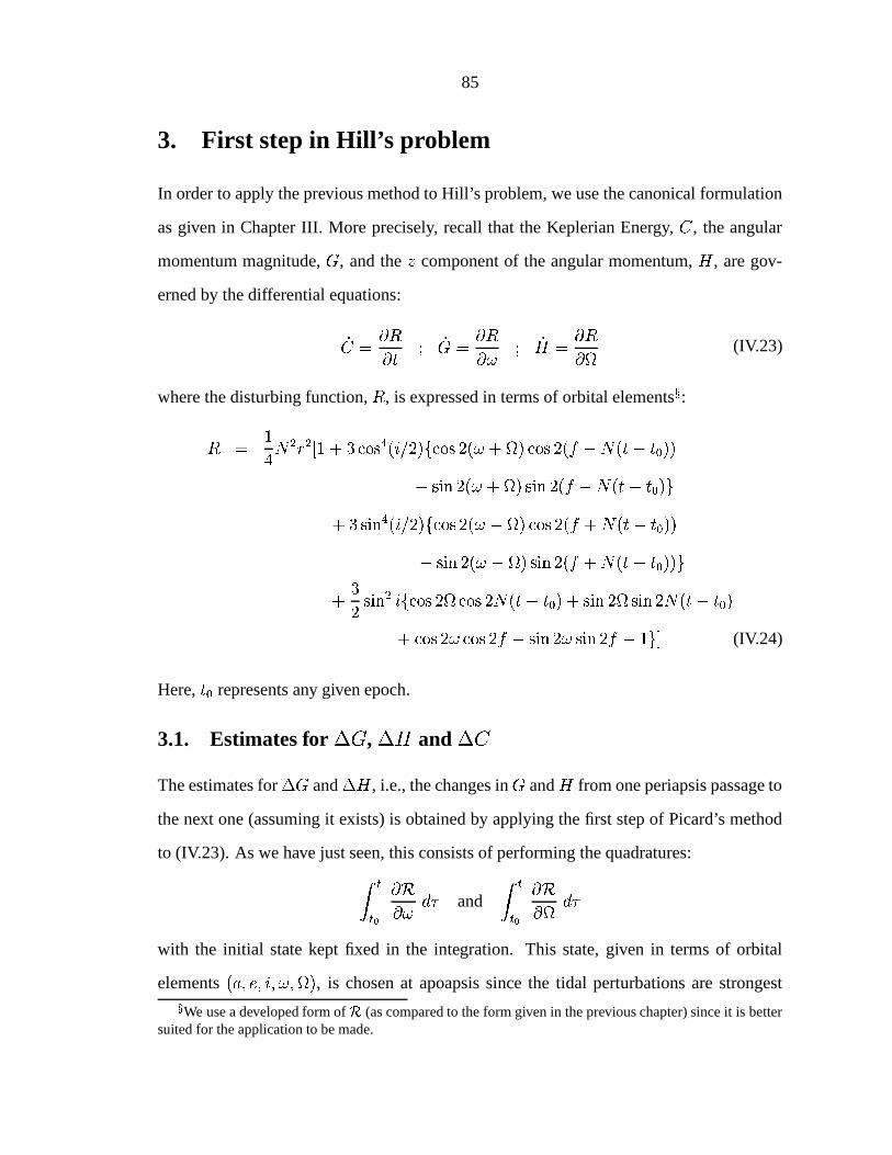
85

3. First step in Hill’s problem

In order to apply the previous method to Hill’s problem, we use the canonical formulation

as given in Chapter III. More precisely, recall that the Keplerian Energy, , the angular

momentum magnitude, , and the component of the angular momentum, , are gov-

erned by the differential equations:

(IV.23)

where the disturbing function, , is expressed in terms of orbital elements:

# ! # "

# " !# ! # "

# " "#

" # "

# (IV.24)

Here, " represents any given epoch.

3.1. Estimates for

,

and

The estimates for and , i.e., the changes in and from one periapsis passage to

the next one (assuming it exists) is obtained by applying the first step of Picard’s method

to (IV.23). As we have just seen, this consists of performing the quadratures:

and

with the initial state kept fixed in the integration. This state, given in terms of orbital

elements , is chosen at apoapsis since the tidal perturbations are strongestWe use a developed form of (as compared to the form given in the previous chapter) since it is better

suited for the application to be made.

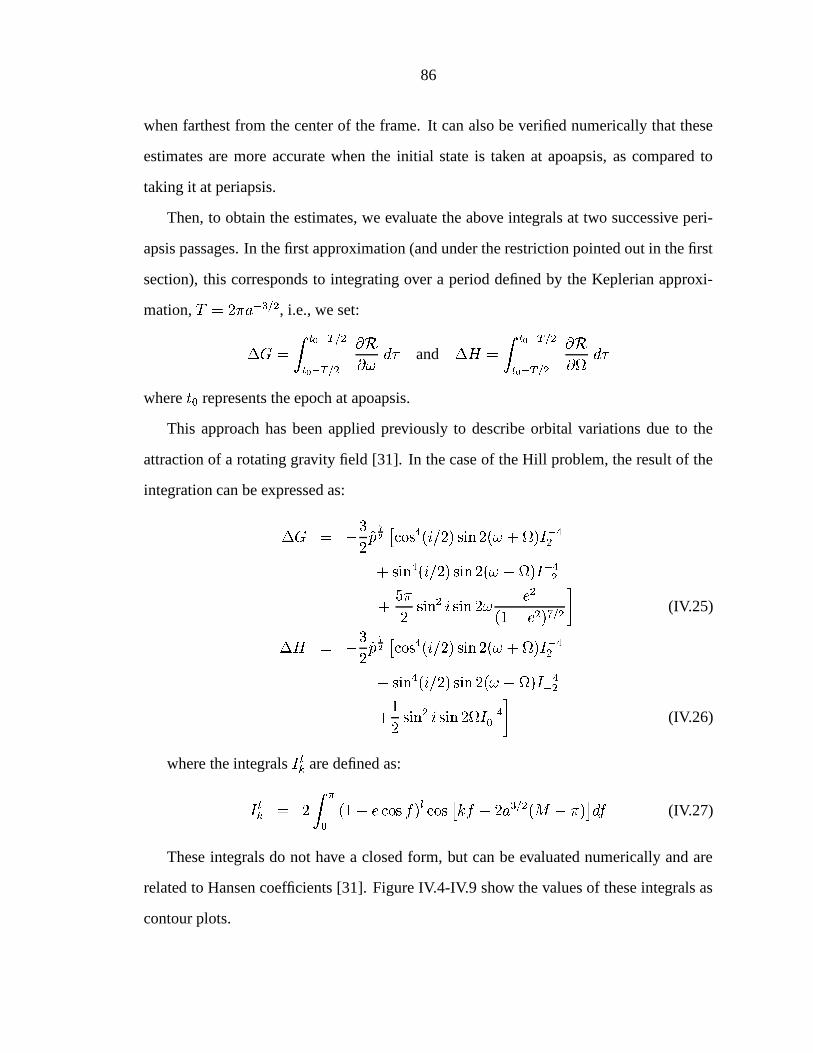
86

when farthest from the center of the frame. It can also be verified numerically that these

estimates are more accurate when the initial state is taken at apoapsis, as compared to

taking it at periapsis.

Then, to obtain the estimates, we evaluate the above integrals at two successive peri-

apsis passages. In the first approximation (and under the restriction pointed out in the first

section), this corresponds to integrating over a period defined by the Keplerian approxi-

mation, , i.e., we set:

and

where " represents the epoch at apoapsis.

This approach has been applied previously to describe orbital variations due to the

attraction of a rotating gravity field [31]. In the case of the Hill problem, the result of the

integration can be expressed as:

# # #

(IV.25)

# # "

(IV.26)

where the integrals are defined as:

" # (IV.27)

These integrals do not have a closed form, but can be evaluated numerically and are

related to Hansen coefficients [31]. Figure IV.4-IV.9 show the values of these integrals as

contour plots.

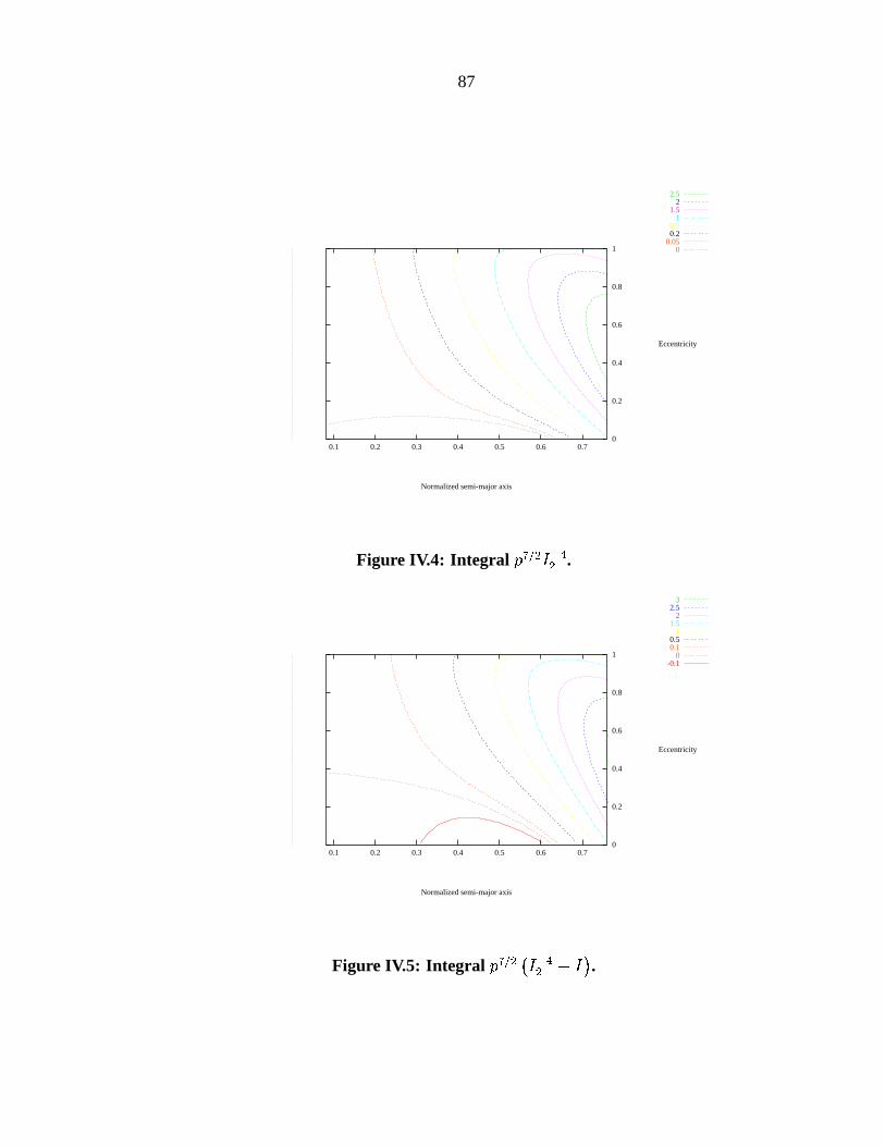
87

2.5 2 1.5 1 0.5 0.2 0.05 0

0.1 0.2 0.3 0.4 0.5 0.6 0.7

Normalized semi-major axis

0

0.2

0.4

0.6

0.8

1

Eccentricity

Figure IV.4: Integral .

3 2.5 2 1.5 1 0.5 0.1 0

-0.1

0.1 0.2 0.3 0.4 0.5 0.6 0.7


0

0.2

0.4

0.6

0.8

1

Eccentricity


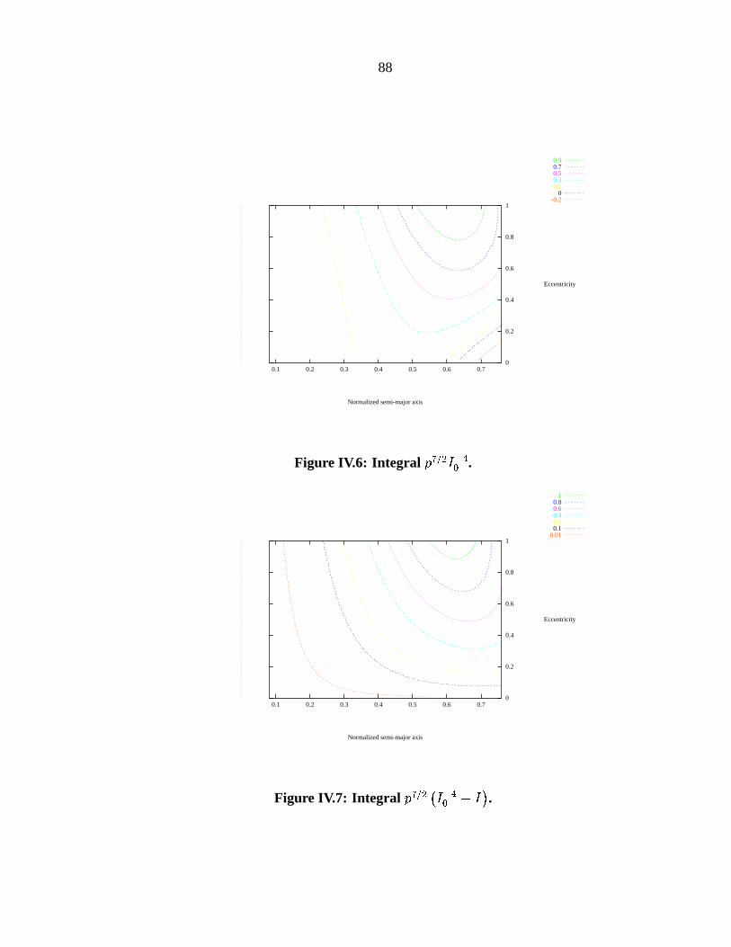
88

0.9 0.7 0.5 0.3 0.1 0

-0.2

0.1 0.2 0.3 0.4 0.5 0.6 0.7


0

0.2

0.4

0.6

0.8

1

Eccentricity

Figure IV.6: Integral " .

1 0.8 0.6 0.4 0.2 0.1 0.01

0.1 0.2 0.3 0.4 0.5 0.6 0.7


0

0.2

0.4

0.6

0.8

1

Eccentricity

Figure IV.7: Integral " .

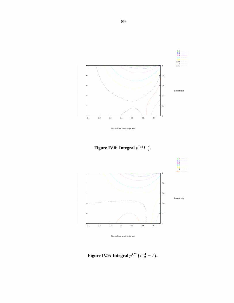
89

0.8 0.6 0.4 0.2 0.1 0.03 0

-0.05

0.1 0.2 0.3 0.4 0.5 0.6 0.7


0

0.2

0.4

0.6

0.8

1

Eccentricity


0.8 0.6 0.4 0.2 0.1 0

-0.1

0.1 0.2 0.3 0.4 0.5 0.6 0.7


0

0.2

0.4

0.6

0.8

1

Eccentricity


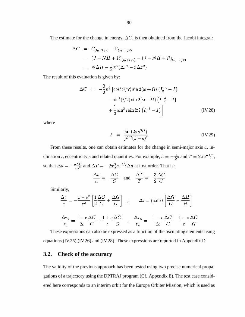
90

The estimate for the change in energy, , is then obtained from the Jacobi integral:

# # # #

The result of this evaluation is given by:

#

# "

(IV.28)

where

# (IV.29)

From these results, one can obtain estimates for the change in semi-major axis , in-

clination , eccentricity and related quantities. For example, and ,so that and at first order. That is:

and

Similarly,

#

;

# #

;

#

These expressions can also be expressed as a function of the osculating elements using

equations (IV.25),(IV.26) and (IV.28). These expressions are reported in Appendix D.

3.2. Check of the accuracy

The validity of the previous approach has been tested using two precise numerical propa-

gations of a trajectory using the DPTRAJ program (Cf. Appendix E). The test case consid-

ered here corresponds to an interim orbit for the Europa Orbiter Mission, which is used as

91

a possible means to lower in the Europa orbit insertion phase of the mission. The ini-

tial conditions are km, and ! at an epoch 05-MAR-2008.

This trajectory impacts the surface of Europa on 12-MAR-2008 after about 12 orbits of

the spacecraft around Jupiter.

From the numerical values of the orbital elements at periapsis and apoapsis, the change

in energy, angular momentum magnitude and its projection on the z-axis has been com-

puted and compared with the values obtained using the analytical expressions. The previ-

ous expressions are then used to calculate the values of the changes in orbital elements.

Table IV.2: Comparison between DPTRAJ and analytical results.

Apoapsis

% error % error error

(km) (km) (deg) (deg) (deg)

A1 6143.77 -162.88 -0.80 0.648 -0.013 -5.08 38.05 14.94 0.52

A2 5822.98 356.95 -0.15 0.524 -0.233 2.66 42.19 -11.78 0.99

A3 5293.84 -8.30 0.06 0.449 -0.012 0.21 36.42 0.66 -0.51

A4 5738.72 -310.06 -0.68 0.559 0.281 0.30 40.91 6.46 0.20

A5 6058.48 111.50 1.23 0.710 0.003 1.96 31.13 -12.56 -3.04

A6 5441.63 228.99 0.25 0.607 -0.280 5.52 29.37 0.63 0.39

A7 5386.55 -203.49 -0.12 0.593 0.254 -4.04 29.27 -0.62 -0.19

A8 6123.58 -180.46 -0.32 0.683 0.014 -6.35 33.23 14.89 1.26

A9 5800.13 351.44 0.27 0.548 -0.253 -0.32 41.63 -9.86 0.68

A10 5301.54 11.76 -0.03 0.447 -0.026 2.11 35.44 -0.54 0.19

A11 5732.30 -314.47 -0.35 0.532 0.257 0.15 40.17 8.92 -0.29

A12 6096.93 65.31 1.52 0.687 0.045 1.08 34.08 -13.69 -2.11

Table IV.2 shows the numerical value of the change (from periapsis to periapsis) in , and together with the percent error made using the analytical theory where the difference

of the changes are normalized by the corresponding quantities at apoapsis. For instance

the percentage error in semi-major axis is defined as where represent the

analytical result, the DPTRAJ result and the value of is taken at the corresponding

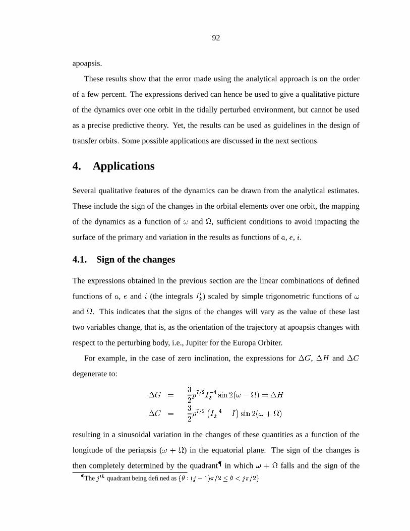
92

apoapsis.

These results show that the error made using the analytical approach is on the order

of a few percent. The expressions derived can hence be used to give a qualitative picture

of the dynamics over one orbit in the tidally perturbed environment, but cannot be used

as a precise predictive theory. Yet, the results can be used as guidelines in the design of

transfer orbits. Some possible applications are discussed in the next sections.

4. Applications

Several qualitative features of the dynamics can be drawn from the analytical estimates.

These include the sign of the changes in the orbital elements over one orbit, the mapping

of the dynamics as a function of and

, sufficient conditions to avoid impacting the

surface of the primary and variation in the results as functions of , , .

4.1. Sign of the changes

The expressions obtained in the previous section are the linear combinations of defined

functions of , and (the integrals ) scaled by simple trigonometric functions of

and

. This indicates that the signs of the changes will vary as the value of these last

two variables change, that is, as the orientation of the trajectory at apoapsis changes with

respect to the perturbing body, i.e., Jupiter for the Europa Orbiter.

For example, in the case of zero inclination, the expressions for , and degenerate to:

#

#

resulting in a sinusoidal variation in the changes of these quantities as a function of the

longitude of the periapsis ( # ) in the equatorial plane. The sign of the changes is

then completely determined by the quadrant in which # falls and the sign of theThe quadrant being defined as $

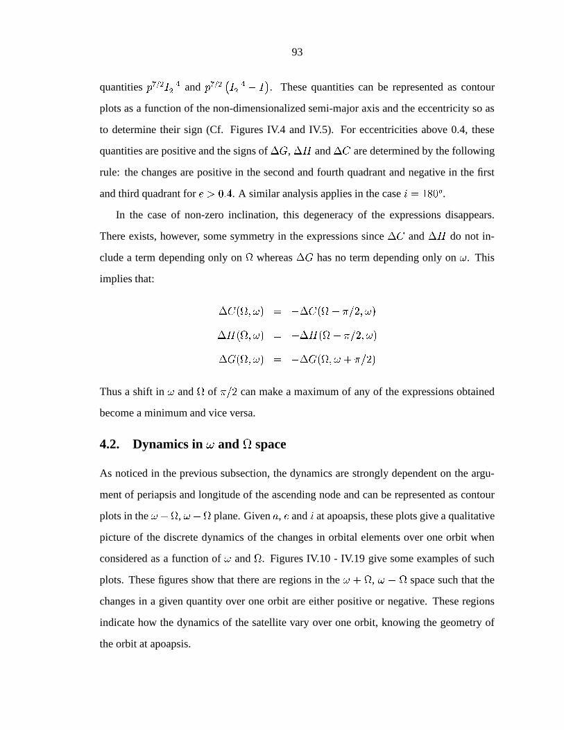
93

quantities and ! . These quantities can be represented as contour

plots as a function of the non-dimensionalized semi-major axis and the eccentricity so as

to determine their sign (Cf. Figures IV.4 and IV.5). For eccentricities above 0.4, these

quantities are positive and the signs of , and are determined by the following

rule: the changes are positive in the second and fourth quadrant and negative in the first

and third quadrant for . A similar analysis applies in the case ! .

In the case of non-zero inclination, this degeneracy of the expressions disappears.

There exists, however, some symmetry in the expressions since and do not in-

clude a term depending only on

whereas has no term depending only on . This

implies that:

# # #

Thus a shift in and

of can make a maximum of any of the expressions obtained

become a minimum and vice versa.

4.2. Dynamics in and

space

As noticed in the previous subsection, the dynamics are strongly dependent on the argu-

ment of periapsis and longitude of the ascending node and can be represented as contour

plots in the # , plane. Given , and at apoapsis, these plots give a qualitative

picture of the discrete dynamics of the changes in orbital elements over one orbit when

considered as a function of and

. Figures IV.10 - IV.19 give some examples of such

plots. These figures show that there are regions in the # , space such that the

changes in a given quantity over one orbit are either positive or negative. These regions

indicate how the dynamics of the satellite vary over one orbit, knowing the geometry of

the orbit at apoapsis.

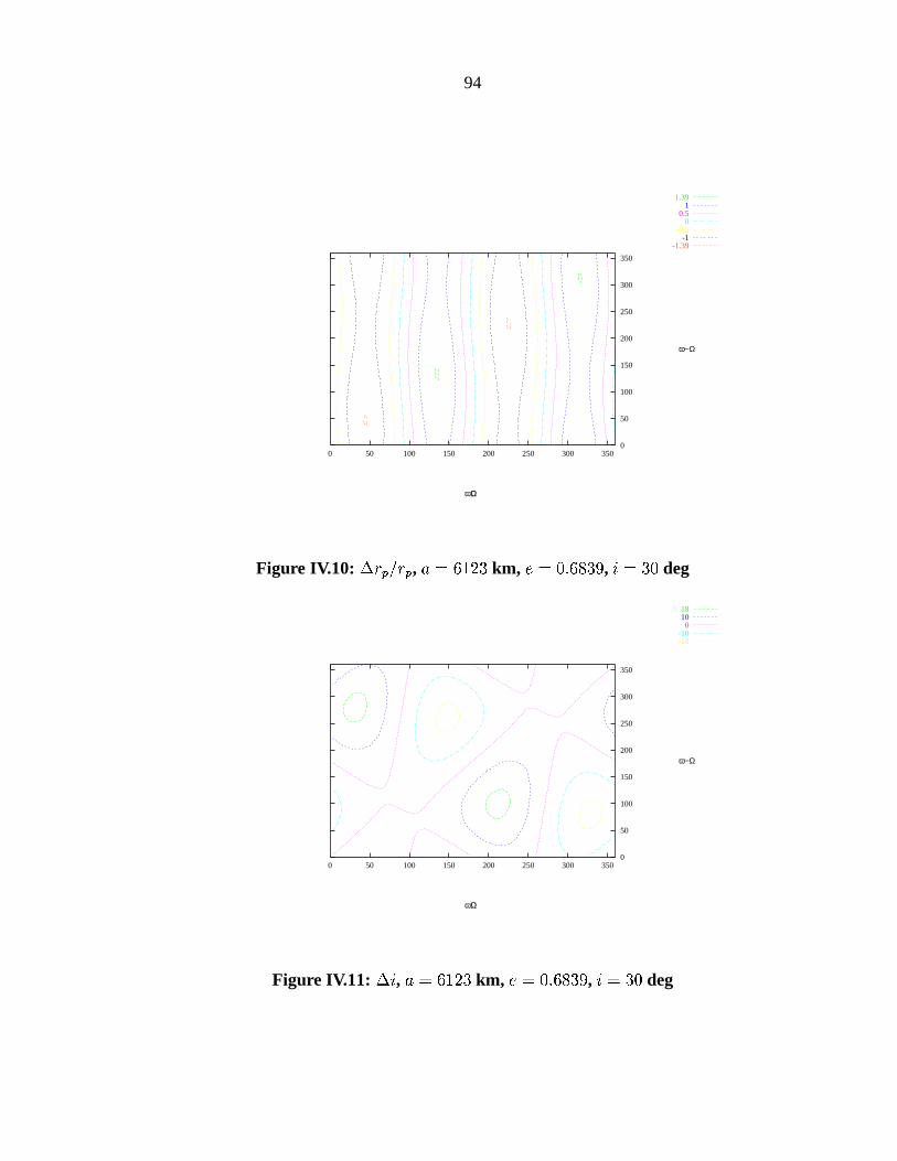
94

1.39 1 0.5 0

-0.5 -1

-1.39

0 50 100 150 200 250 300 350

ω+Ω

0

50

100

150

200

250

300

350

ω−Ω

Figure IV.10: , km, , deg

18 10 0

-10 -18

0 50 100 150 200 250 300 350

ω+Ω

0

50

100

150

200

250

300

350

ω−Ω


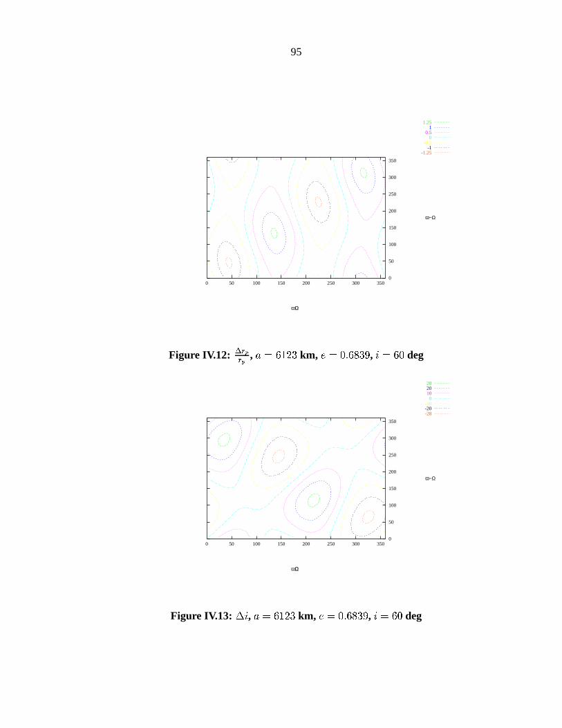
95

1.25 1 0.5 0

-0.5 -1

-1.25

0 50 100 150 200 250 300 350

ω+Ω

0

50

100

150

200

250

300

350

ω−Ω


28 20 10 0

-10 -20 -28

0 50 100 150 200 250 300 350

ω+Ω

0

50

100

150

200

250

300

350

ω−Ω


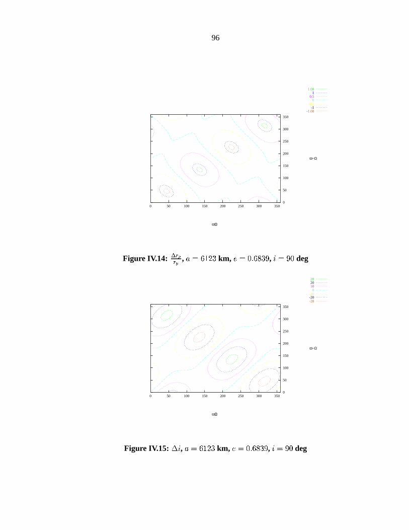
96

1.08 1 0.5 0

-0.5 -1

-1.08

0 50 100 150 200 250 300 350

ω+Ω

0

50

100

150

200

250

300

350

ω−Ω


28 20 10 0

-10 -20 -28

0 50 100 150 200 250 300 350

ω+Ω

0

50

100

150

200

250

300

350

ω−Ω


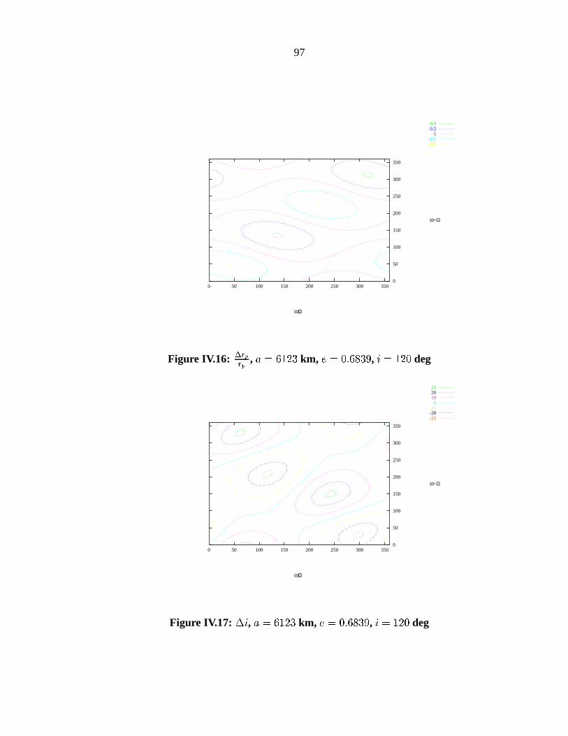
97

0.9 0.5 0

-0.5 -0.9

0 50 100 150 200 250 300 350

ω+Ω

0

50

100

150

200

250

300

350

ω−Ω


25 20 10 0

-10 -20 -25

0 50 100 150 200 250 300 350

ω+Ω

0

50

100

150

200

250

300

350

ω−Ω


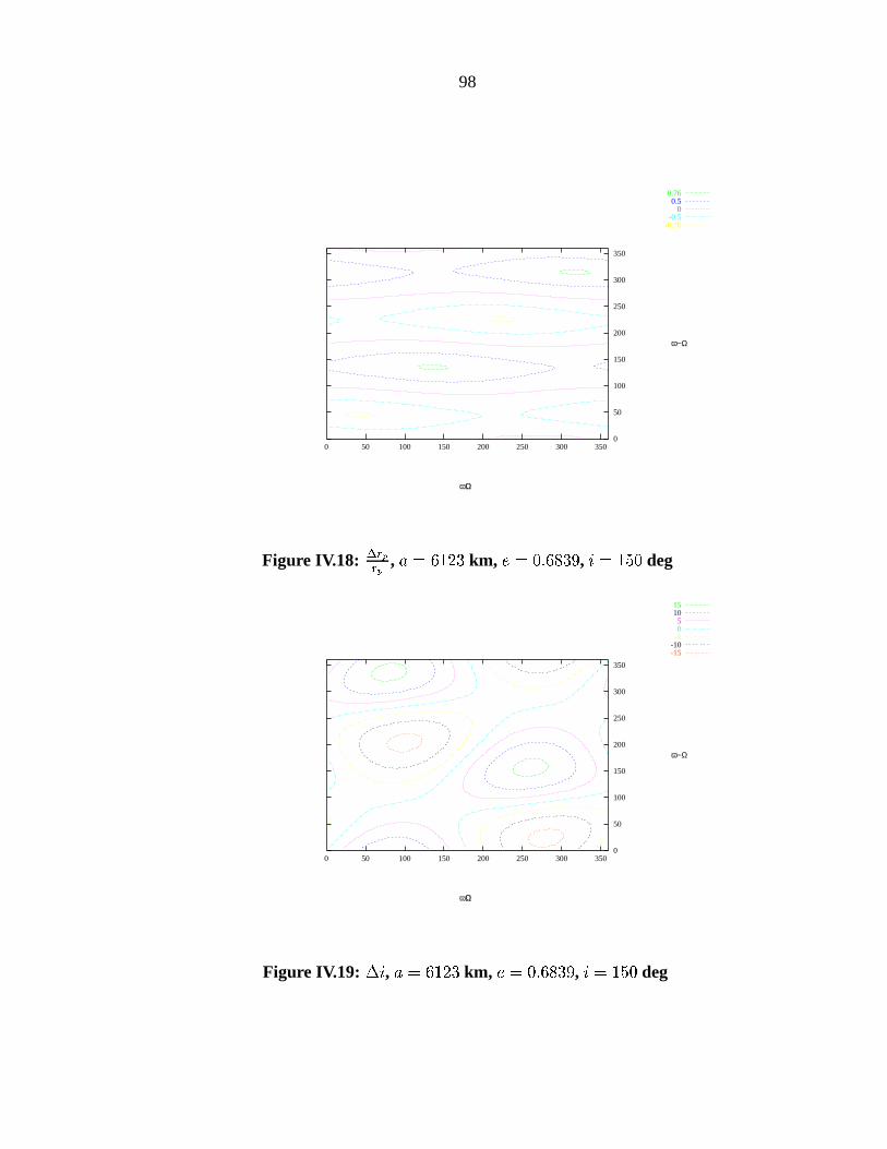
98

0.76 0.5 0

-0.5 -0.76

0 50 100 150 200 250 300 350

ω+Ω

0

50

100

150

200

250

300

350

ω−Ω


15 10 5 0 -5 -10 -15

0 50 100 150 200 250 300 350

ω+Ω

0

50

100

150

200

250

300

350

ω−Ω


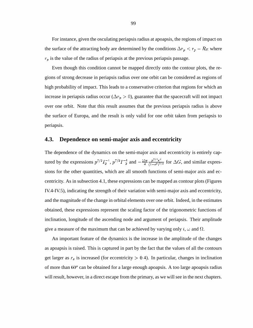
99

For instance, given the osculating periapsis radius at apoapsis, the regions of impact on

the surface of the attracting body are determined by the conditions where

is the value of the radius of periapsis at the previous periapsis passage.

Even though this condition cannot be mapped directly onto the contour plots, the re-

gions of strong decrease in periapsis radius over one orbit can be considered as regions of

high probability of impact. This leads to a conservative criterion that regions for which an

increase in periapsis radius occur ( ), guarantee that the spacecraft will not impact

over one orbit. Note that this result assumes that the previous periapsis radius is above

the surface of Europa, and the result is only valid for one orbit taken from periapsis to

periapsis.

4.3. Dependence on semi-major axis and eccentricity

The dependence of the dynamics on the semi-major axis and eccentricity is entirely cap-

tured by the expressions , and

for , and similar expres-

sions for the other quantities, which are all smooth functions of semi-major axis and ec-

centricity. As in subsection 4.1, these expressions can be mapped as contour plots (Figures

IV.4-IV.5), indicating the strength of their variation with semi-major axis and eccentricity,

and the magnitude of the change in orbital elements over one orbit. Indeed, in the estimates

obtained, these expressions represent the scaling factor of the trigonometric functions of

inclination, longitude of the ascending node and argument of periapsis. Their amplitude

give a measure of the maximum that can be achieved by varying only , and

.

An important feature of the dynamics is the increase in the amplitude of the changes

as apoapsis is raised. This is captured in part by the fact that the values of all the contours

get larger as is increased (for eccentricity ). In particular, changes in inclination

of more than ! can be obtained for a large enough apoapsis. A too large apoapsis radius

will result, however, in a direct escape from the primary, as we will see in the next chapters.

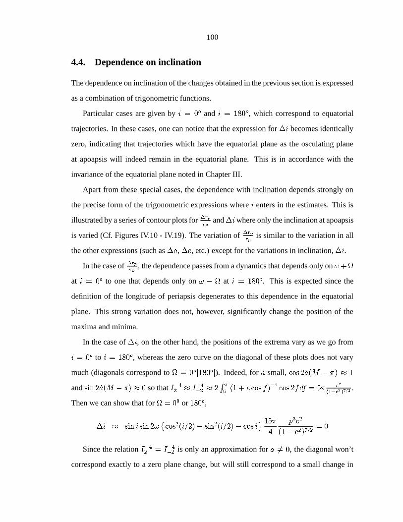
100

4.4. Dependence on inclination

The dependence on inclination of the changes obtained in the previous section is expressed

as a combination of trigonometric functions.

Particular cases are given by ! and ! , which correspond to equatorial

trajectories. In these cases, one can notice that the expression for becomes identically

zero, indicating that trajectories which have the equatorial plane as the osculating plane

at apoapsis will indeed remain in the equatorial plane. This is in accordance with the

invariance of the equatorial plane noted in Chapter III.

Apart from these special cases, the dependence with inclination depends strongly on

the precise form of the trigonometric expressions where enters in the estimates. This is

illustrated by a series of contour plots for and where only the inclination at apoapsis

is varied (Cf. Figures IV.10 - IV.19). The variation of is similar to the variation in all

the other expressions (such as , , etc.) except for the variations in inclination, .In the case of , the dependence passes from a dynamics that depends only on #

at ! to one that depends only on at ! . This is expected since the

definition of the longitude of periapsis degenerates to this dependence in the equatorial

plane. This strong variation does not, however, significantly change the position of the

maxima and minima.

In the case of , on the other hand, the positions of the extrema vary as we go from

! to ! , whereas the zero curve on the diagonal of these plots does not vary

much (diagonals correspond to ! ! ). Indeed, for

small,

and so that " #

.

Then we can show that for

"or ! ,

Since the relation is only an approximation for , the diagonal won’t

correspond exactly to a zero plane change, but will still correspond to a small change in

101

inclination. This holds as long as remains small ( ) and the eccentricity is not too

high ( ).

All these examples show that the dependence on inclination is strong enough to make

the signs of the estimates change over relatively large regions (in the space) but still

too weak to transform a maximum into a minimum, as opposed to the variations obtained

with and

.

The next two chapters describe two practical applications resulting from these dynam-

ics: plane changes and escape/capture maneuvers in an environment perturbed by a third

body.

CHAPTER V

THIRD BODY DRIVEN PLANE CHANGES

This chapter builds on the insights of the two previous chapters by presenting a new class

of plane change maneuvers in a body perturbed environment [40, 39].

As was noted in the introduction of the dissertation, this topic was first motivated by

the Europa Orbiter Mission. Indeed, we have seen in Chapter III that low altitude, nearly

circular, polar orbits are unstable, with instabilities on the order of weeks for the case of

Europa. These polar orbits are interesting scientifically since they allow us to map the high

latitude regions of the satellite, a necessary ingredient in some scientific investigations.

Placing a spacecraft on such a trajectory requires periodic control maneuvers to avoid an

impact with Europa. Such maneuvers are expensive over long time spans, and it seems

preferable to transfer the spacecraft into a low inclination, stable orbit to avoid impacts

over long intervals of time. Such transfers involve a large plane change maneuver (which

is a very expensive maneuver). Minimizing the cost of such a transfer is an important goal.

Also, the topic of plane change maneuvers has its own dynamical interest since it in-

volves, intrinsically, the full -dimensional dynamics and a nontrivial comparison with

classical strategies. Indeed, as we will review in the first section, the optimal classic strat-

egy for plane changes below ! is obtained with a one impulse maneuver. This ma-

neuver is still applicable in a body perturbed environment since it does not involve a

transfer trajectory with a large apoapsis radius. Thus, the question of the optimal plane

change strategy arises. This question has a beautiful answer found with the help of the

Jacobi constant, which allows us to obtain tight bounds on the limits of optimality. This is

102

103

derived in Section .

Section looks at the third body driven plane changes, without concern about the cost

of the transfers. In particular, the problem is formulated as a non-convex optimization

problem for which a numerical approach is proposed.

1. Classic vs. third body driven transfers

Classically, the design of orbit transfers is based on the two body problem for the underly-

ing dynamics. In this model, the trajectory of a spacecraft is entirely determined by its five

orbital elements: semi-major axis , eccentricity , inclination , longitude of the ascend-

ing node

and argument of periapsis . In this situation, relations between two points on a

given orbit are readily obtained and the problem of determining a transfer can be viewed as

a geometrical problem of the intersection of conics together with an optimization over all

possible impulsive maneuvers. In particular, there is no distinction between the dynamics

on the initial, final, and transfer orbits. The time appears as a secondary variable (possibly

as a cost function) in the sense that if a transfer is possible at time " , it is also possible at

time " # where represents the period of motion on the initial orbit. Also, the absolute

position of the initial and final orbits relative to a given inertial frame are not generally

taken into account in the formulation of the problem, only the relative orientation of the

initial orbit with respect to the final one is important. A typical example of transfer is

given by the bi-elliptic plane change (or restricted three impulse plane change [7]), where

a spacecraft starts in an initial low altitude, circular orbit, a first maneuver transfers it to an

ellipse where a second maneuver is performed at apoapsis, changing its orbital plane, and

a final maneuver at the next periapsis re-transfers the spacecraft to a low altitude, circular

orbit (see Figure V.1).

When perturbations occur, however, this state of affairs changes. Orbital elements are

now a function of time and there may be no definite analytical relationship between two

points on a given orbit. The situation is not so bad for small perturbations where averaging

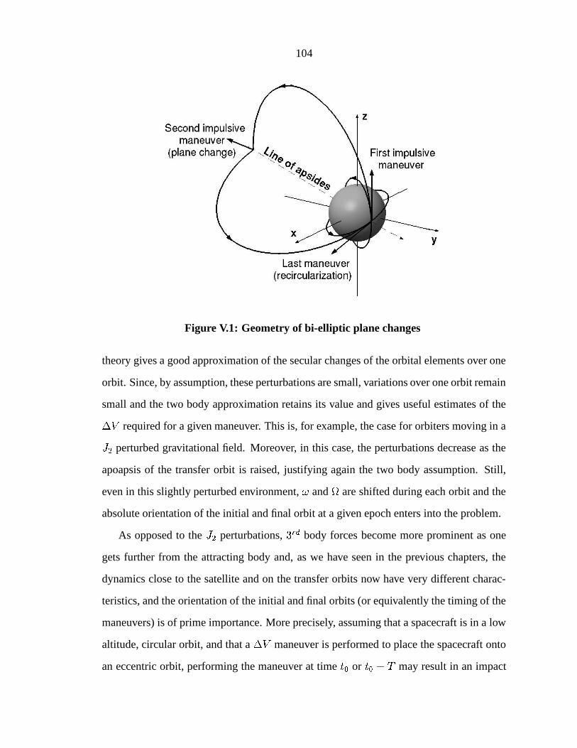
104

Figure V.1: Geometry of bi-elliptic plane changes

theory gives a good approximation of the secular changes of the orbital elements over one

orbit. Since, by assumption, these perturbations are small, variations over one orbit remain

small and the two body approximation retains its value and gives useful estimates of the

required for a given maneuver. This is, for example, the case for orbiters moving in a

perturbed gravitational field. Moreover, in this case, the perturbations decrease as the

apoapsis of the transfer orbit is raised, justifying again the two body assumption. Still,

even in this slightly perturbed environment, and

are shifted during each orbit and the

absolute orientation of the initial and final orbit at a given epoch enters into the problem.

As opposed to the perturbations, body forces become more prominent as one

gets further from the attracting body and, as we have seen in the previous chapters, the

dynamics close to the satellite and on the transfer orbits now have very different charac-

teristics, and the orientation of the initial and final orbits (or equivalently the timing of the

maneuvers) is of prime importance. More precisely, assuming that a spacecraft is in a low

altitude, circular orbit, and that a maneuver is performed to place the spacecraft onto

an eccentric orbit, performing the maneuver at time " or " # may result in an impact

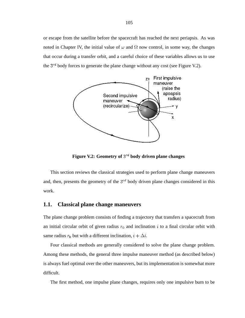
105

or escape from the satellite before the spacecraft has reached the next periapsis. As was

noted in Chapter IV, the initial value of and

now control, in some way, the changes

that occur during a transfer orbit, and a careful choice of these variables allows us to use

the body forces to generate the plane change without any cost (see Figure V.2).

Figure V.2: Geometry of body driven plane changes

This section reviews the classical strategies used to perform plane change maneuvers

and, then, presents the geometry of the body driven plane changes considered in this

work.

1.1. Classical plane change maneuvers

The plane change problem consists of finding a trajectory that transfers a spacecraft from

an initial circular orbit of given radius " and inclination to a final circular orbit with

same radius " but with a different inclination, # .Four classical methods are generally considered to solve the plane change problem.

Among these methods, the general three impulse maneuver method (as described below)

is always fuel optimal over the other maneuvers, but its implementation is somewhat more

difficult.

The first method, one impulse plane changes, requires only one impulsive burn to be

106

performed at one of the nodes of the orbit (i.e., at the crossing with the equatorial plane).

This maneuver consists of rotating the velocity vector by the desired amount of the plane

change. Thus, its cost is given by:

(V.1)

where is the local circular velocity speed at the time of the maneuver. This

method is easy to implement and is cheaper than bi-elliptic and parabolic maneuvers for

plane changes less than ! .Above this value, bi-elliptic maneuvers become less expensive. These maneuvers con-

sist of first placing the spacecraft on an elliptic trajectory in order to raise the apoapsis

radius. When apoapsis is reached, the one impulse plane change is performed so as to

obtain the desired plane change. At the next periapsis, the spacecraft is inserted into the

final circular orbit. The idea behind this transfer is that decreases with an increase in so that decreases with an increase in , as well. Performing the plane change

at apoapsis results in decreased costs. This first and third burn are simply tangent to the

path. This method is illustrated in Figure V.1. The cost of these maneuvers is given by:

#

(V.2)

where is the ratio of the apoapsis radius of the transfer ellipse to the radius of the initial

circular orbit. The optimal choice for this parameter (i.e., the choice which results in the

minimization of for a given ) is given by .From this formula, we can easily see that for ! , # . Thus, starting at

! , plane change are cheaper if we let the spacecraft fly off to ‘infinity’ and perform

the plane change at ‘infinity’, where its cost is zero. The cost of the maneuver is, in fact,

contained in the first and last burns which correspond to escape and capture maneuvers.

From a practical point of view, this result indicates that for large plane change values, the

farther the apoapsis of the transfer trajectory is, the cheaper is the maneuver. The cost of

107

the ideal maneuver is:

(V.3)

Note that the optimal solution of the general three impulse plane change, which con-

sists of performing plane change maneuvers at each burn of a bi-elliptic transfer, merges

with the parabolic result at the same value of ! as for bi-elliptic transfers. No

analytical expression is available for the costs of these transfers as a function of the initial

conditions [7].

Thus, we can see from these results, that large plane change maneuvers require sig-

nificantly raising the apoapsis to perform the transfer and that these maneuvers are very

expensive.

As was noted in the introduction of this section, in a body framework, raising the

apoapsis cannot be performed without incurring large changes on all the orbital elements

and, among the classical methods discussed above, only the one impulse maneuvers can

still be directly applied in such orbital environments.

The next subsection explains a way to take advantage of these dynamics to decrease

the cost of plane change maneuvers.

1.2. Third body driven plane changes

The idea of body driven transfers is to place the spacecraft into a highly eccentric

transfer trajectory (to raise the apoapsis radius) so that the large body forces can per-

form plane change maneuvers without any costs at apoapsis. That is, the body

driven plane changes considered here are analogous to bi-elliptic plane changes, with the

apoapsis maneuver replaced by the “cost free” action of the third body forces.

More precisely, when the spacecraft moves along an initial, low altitude, circular orbit,

we have seen in Chapter III that the mean anomaly, , and the longitude of the ascending

node,

, can be approximated by linear functions of time and can be represented as a line

108

wrapping in the -torus space (all the other orbital elements remaining fixed during

the motion by our approximation of circular motion).

A tangential impulsive maneuver at any point of this initial circular orbit will place

the spacecraft at the periapsis of a transfer trajectory, the orbital elements of which are

determined using the following correspondences :

Initial, circular orbit Transfer trajectory

(V.4)

where represents the mean motion of the spacecraft on the initial circular

orbit. In particular, and

are directly related to the value of and

of the initial

circular orbit and their values vary as we let the spacecraft move along the initial circular

orbit.

Now, numerical integration of the flow up to the next periapsis as and

are varied

( , , being fixed) allows us to map all the possible transfer trajectories from this

initial circular orbit and obtain a simple geometric representation of the change in orbital

elements over a transfer trajectory. That is, we numerically compute a periapsis Poincaré

map with the initial elements taken at periapsis (see Figure V.3).

The existence of curves indicates that for an appropriate choice of and

of the transfer trajectory, a zero change in periapsis radius will result at the next periapsis

passage. If is non zero for this given value of and

, a recircularization maneuver at

the next periapsis passage will correspond to the completion of a plane change maneuver.

Figure V.2 shows a numerically integrated trajectory corresponding to the design of such

a third body driven plane change for ! . !! corresponds to the apoapsis radisu obtained from a tangemtial burn,

starting in a circular orbit.

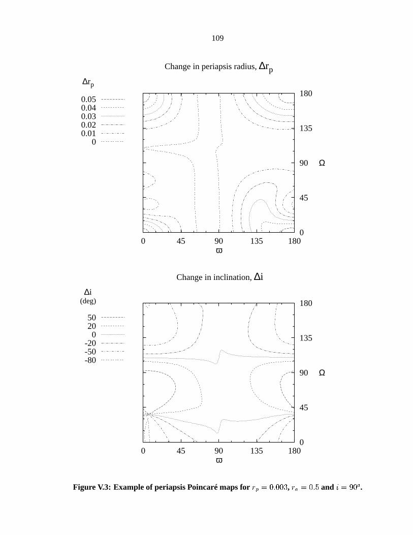
109

Change in periapsis radius, ∆rp

∆rp

0.05 0.04 0.03 0.02 0.01 0

0 45 90 135 180ω

0

45

90

135

180

Ω

Change in inclination, ∆i

∆i (deg)

50 20 0

-20 -50 -80

0 45 90 135 180ω

0

45

90

135

180

Ω

Figure V.3: Example of periapsis Poincaré maps for , " and ! .

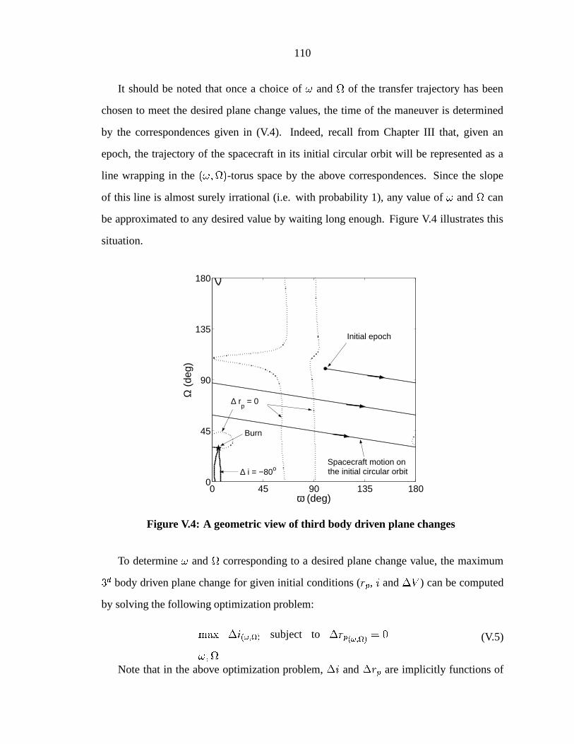
110

It should be noted that once a choice of and

of the transfer trajectory has been

chosen to meet the desired plane change values, the time of the maneuver is determined

by the correspondences given in (V.4). Indeed, recall from Chapter III that, given an

epoch, the trajectory of the spacecraft in its initial circular orbit will be represented as a

line wrapping in the -torus space by the above correspondences. Since the slope

of this line is almost surely irrational (i.e. with probability 1), any value of and

can

be approximated to any desired value by waiting long enough. Figure V.4 illustrates this

situation.

0 45 90 135 1800

45

90

135

180

ω (deg)

Ω (

deg)

∆ rp = 0

∆ i = −80o

Burn

Initial epoch

Spacecraft motion on the initial circular orbit

Figure V.4: A geometric view of third body driven plane changes

To determine and

corresponding to a desired plane change value, the maximum

body driven plane change for given initial conditions ( , and ) can be computed

by solving the following optimization problem:

subject to

(V.5)

Note that in the above optimization problem, and are implicitly functions of

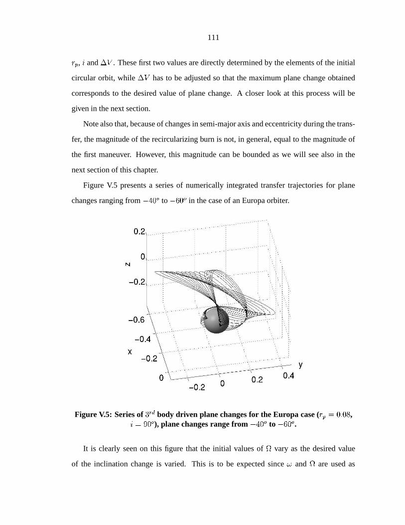
111

, and . These first two values are directly determined by the elements of the initial

circular orbit, while has to be adjusted so that the maximum plane change obtained

corresponds to the desired value of plane change. A closer look at this process will be

given in the next section.

Note also that, because of changes in semi-major axis and eccentricity during the trans-

fer, the magnitude of the recircularizing burn is not, in general, equal to the magnitude of

the first maneuver. However, this magnitude can be bounded as we will see also in the

next section of this chapter.

Figure V.5 presents a series of numerically integrated transfer trajectories for plane

changes ranging from ! to ! in the case of an Europa orbiter.

Figure V.5: Series of body driven plane changes for the Europa case ( , ! ), plane changes range from

! to ! .

It is clearly seen on this figure that the initial values of

vary as the desired value

of the inclination change is varied. This is to be expected since and

are used as

112

control variables and their values are fixed by the amount of plane change to be performed.

Moreover, their values at the next periapsis are also fixed, showing the lack of direct control

of the longitude of the ascending node on the final orbit. However, since

precesses in

this environment, phasing methods can be used to achieve specific values of " at a given

epoch.

2. Fuel unconstrained problem

The above discussion shows that body driven plane changes can be computed by solv-

ing an optimization problem over the Poincaré sections defined by the periapsis condi-

tions. More precisely, we just have seen that the values of and

that yield a desired

plane change are computed by solving the maximum and minimum values of plane change

realizable for a given value of initial inclination, periapsis and apoapsis radii (i.e. ).

That is, we solve the following non-convex optimization problem:

(V.6)

This section presents a numerical algorithm to solve this problem, as well as the results

of the computation. As it turns out, this problem will allow us to solve a more complex

problem formulated in the next section.

2.1. Numerical solution for the maximum and minimum plane change

Even though the above problem can a priori be solved by standard optimization algorithms,

the numerical procedure used in this dissertation consists of first searching the zero

lines on the torus ! ! and then looking for the maximum plane change on

these zero lines. This method has the advantage of not necessitating an initial guess while

allowing us to keep track of the zero lines.

The search for the lines is performed by first searching the crossings of the

lines with the axes ! and ! and then tracking the zero lines from these points.

Resp.

$ for the minimum plane change.

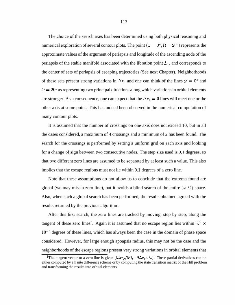
113

The choice of the search axes has been determined using both physical reasoning and

numerical exploration of several contour plots. The point ! ! represents the

approximate values of the argument of periapsis and longitude of the ascending node of the

periapsis of the stable manifold associated with the libration point , and corresponds to

the center of sets of periapsis of escaping trajectories (See next Chapter). Neighborhoods

of these sets present strong variations in and one can think of the lines ! and ! as representing two principal directions along which variations in orbital elements

are stronger. As a consequence, one can expect that the lines will meet one or the

other axis at some point. This has indeed been observed in the numerical computation of

many contour plots.

It is assumed that the number of crossings on one axis does not exceed 10, but in all

the cases considered, a maximum of 4 crossings and a minimum of 2 has been found. The

search for the crossings is performed by setting a uniform grid on each axis and looking

for a change of sign between two consecutive nodes. The step size used is degrees, so

that two different zero lines are assumed to be separated by at least such a value. This also

implies that the escape regions must not lie within degrees of a zero line.

Note that these assumptions do not allow us to conclude that the extrema found are

global (we may miss a zero line), but it avoids a blind search of the entire -space.

Also, when such a global search has been performed, the results obtained agreed with the

results returned by the previous algorithm.

After this first search, the zero lines are tracked by moving, step by step, along the

tangent of these zero lines

. Again it is assumed that no escape region lies within degrees of these lines, which has always been the case in the domain of phase space

considered. However, for large enough apoapsis radius, this may not be the case and the

neighborhoods of the escape regions present very strong variations in orbital elements thatThe tangent vector to a zero line is given . These partial derivatives can be

either computed by a finite difference scheme or by computing the state transition matrix of the Hill problemand transforming the results into orbital elements.

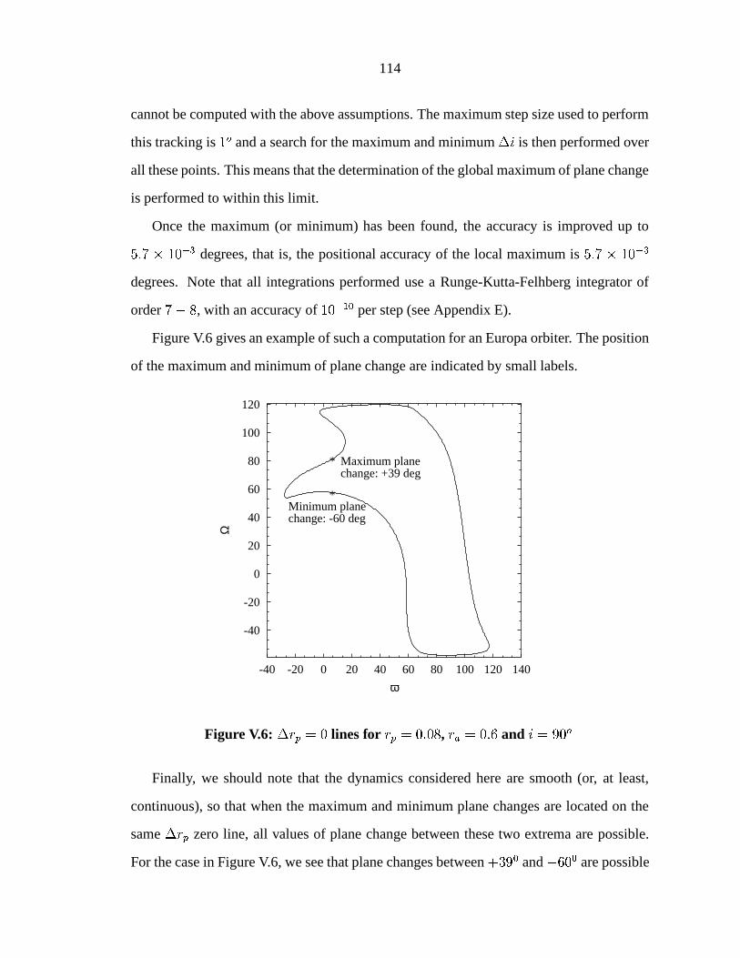
114

cannot be computed with the above assumptions. The maximum step size used to perform

this tracking is ! and a search for the maximum and minimum is then performed over

all these points. This means that the determination of the global maximum of plane change

is performed to within this limit.

Once the maximum (or minimum) has been found, the accuracy is improved up to

degrees, that is, the positional accuracy of the local maximum is

degrees. Note that all integrations performed use a Runge-Kutta-Felhberg integrator of

order , with an accuracy of "

per step (see Appendix E).

Figure V.6 gives an example of such a computation for an Europa orbiter. The position

of the maximum and minimum of plane change are indicated by small labels.

-40

-20

0

20

40

60

80

100

120

-40 -20 0 20 40 60 80 100 120 140

Ω

ω

* Maximum planechange: +39 deg

*Minimum planechange: -60 deg

Figure V.6: lines for , and !

Finally, we should note that the dynamics considered here are smooth (or, at least,

continuous), so that when the maximum and minimum plane changes are located on the

same zero line, all values of plane change between these two extrema are possible.

For the case in Figure V.6, we see that plane changes between # " and " are possible

115

by timing the initial impulsive maneuver. For other cases, such as ! plane changes

indicated in the next subsection, the maximum and minimum plane changes are located

on two different, separated zero lines and not all the values of plane change between these

extrema are realizable.

2.2. Variations with the initial conditions

Once this computation has been performed for a given set of values of periapsis radius,

apoapsis radius, and inclination, the algorithm is repeated to cover a wide range of cases.

Figures V.7 to V.11 give the results of such computations when, respectively, the initial

inclination, apoapsis radius and periapsis radius are varied. Each plot has been computed

with at least points for the independent variable.

Variations with initial inclination

Two distinct behaviors of the variations of the minimum plane change are obtained when

inclination varies, according to the initial values of periapsis radius, , and apoapsis ra-

dius, .

For the lower values of apoapsis radius (at fixed ), the minimum and maximum plane

changes obtained for the inclinations of ! and ! are zero. In this case, the changes in

orbital elements become larger around an inclination of ! as can be seen on Figure V.7

for the change in inclination.

For higher values of apoapsis radius (or lower values of periapsis radius with fixed ),

a bifurcation occurs, so that, at the inclinations of ! and ! , a maximum and minimum

plane change of ! and ! , respectively, are obtained, as can be seen in Figures V.8

and V.9. Note that this result is consistent with the invariance of the -plane in the

Hill problem. A plane change of ! at an inclination of ! or ! corresponds, indeed,Tags on these graphs are explained in the next subsectionOnly plane changes of $ $ are possible with the initial conditions chosen for Figure V.8. Plane

changes of $ $ are possible for higher apoapsis radii (e.g. $ ), but some zero lines cannot becomputed at such a high value of with the present program.

116

-60

-50

-40

-30

-20

-10

0

10

20

30

0 45 90 135 180

Plan

e ch

ange

(de

g)

Inclination (deg)

Critical points*

i=73o

∆i=-37o *i=125o

∆i=-37o

xSavings = 26.8%(i=100o, ∆i=-52o)

+ ∆i=+27o

(i=56o, no savings)

Figure V.7: Extrema values of plane change as a function of inclination ( , " )

to a change in the direction of motion relative to the primary (change from retrograde to

direct orbit or vice versa), and does not involve any -component of the velocity vector.

The motion remains planar during such a transfer. Further results on these transfers are

given in the next section.

These figures also show that the bifurcations for positive and negative plane changes

do not necessarily occur for the same values of periapsis and apoapsis radii. The few

numerical explorations performed suggest that the bifurcation for negative plane changes

occurs at lower values of apoapsis radius than that for positive plane changes. In fact, as

it clearly appears in Figures V.7 to V.11, the dynamics are not symmetric for positive and

negative plane changes, even though there are some similarities. It seems that at any value

of and , the overall maximum plane change realizable (i.e., over all initial inclinations)

is less than the overall negative plane change possible (in absolute value).

In the rest of this subsection, an inclination of ! has been assumed as a representative

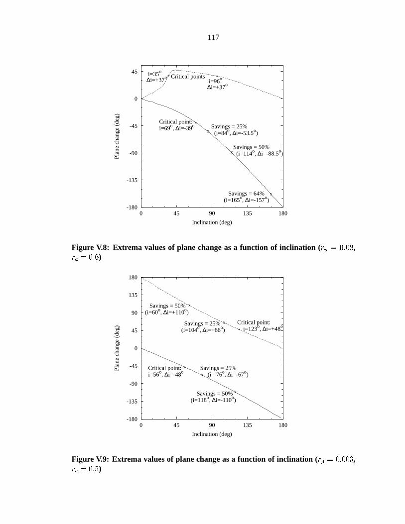
117

-180

-135

-90

-45

0

45

0 45 90 135 180

Plan

e ch

ange

(de

g)

Inclination (deg)

Critical points* i=35o

∆i=+37o * i=96o

∆i=+37o

*Critical point:i=69o, ∆i=-39o

xSavings = 25% (i=84o, ∆i=-53.5o)

xSavings = 50% (i=114o, ∆i=-88.5o)

x Savings = 64%(i=165o, ∆i=-157o)

Figure V.8: Extrema values of plane change as a function of inclination ( , )

-180

-135

-90

-45

0

45

90

135

180

0 45 90 135 180

Plan

e ch

ange

(de

g)

Inclination (deg)

*

Critical point: i=123o, ∆i=+48o

x Savings = 25%(i=104o, ∆i=+66o)

x Savings = 50%(i=60o, ∆i=+110o)

*Critical point:i=56o, ∆i=-48o

xSavings = 25% (i =76o, ∆i=-67o)

x Savings = 50%(i=118o, ∆i=-110o)

Figure V.9: Extrema values of plane change as a function of inclination ( , " )

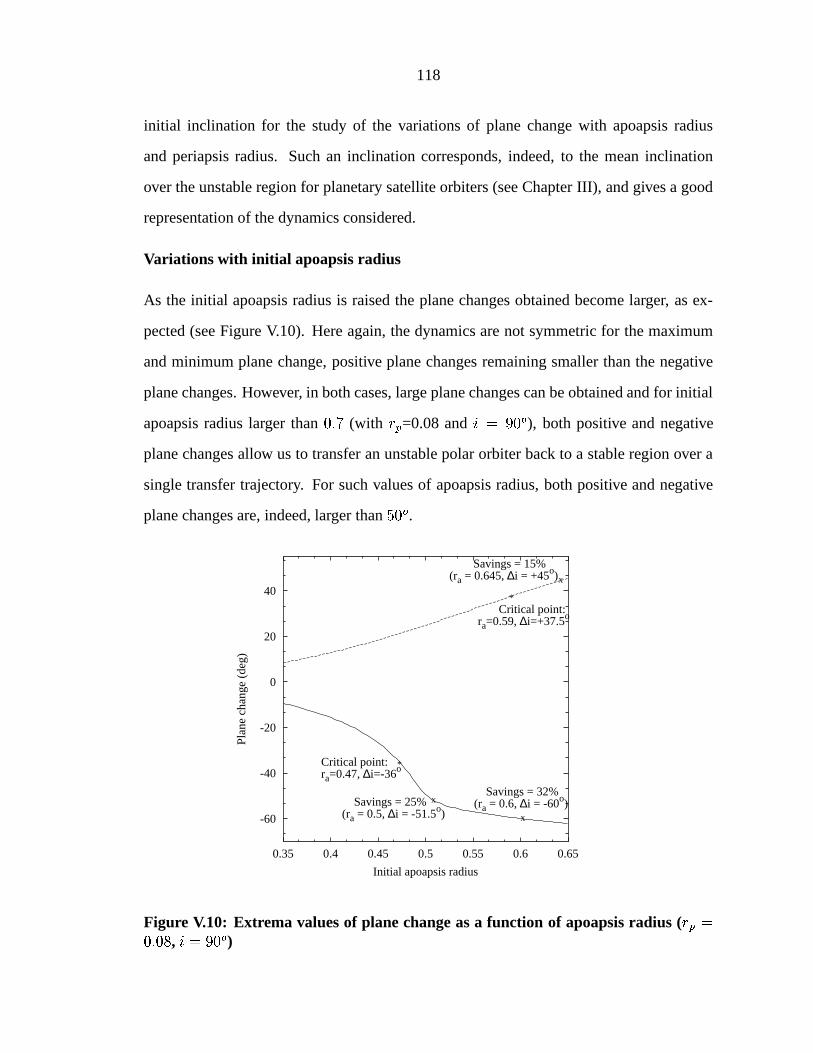
118

initial inclination for the study of the variations of plane change with apoapsis radius

and periapsis radius. Such an inclination corresponds, indeed, to the mean inclination

over the unstable region for planetary satellite orbiters (see Chapter III), and gives a good

representation of the dynamics considered.

Variations with initial apoapsis radius

As the initial apoapsis radius is raised the plane changes obtained become larger, as ex-

pected (see Figure V.10). Here again, the dynamics are not symmetric for the maximum

and minimum plane change, positive plane changes remaining smaller than the negative

plane changes. However, in both cases, large plane changes can be obtained and for initial

apoapsis radius larger than (with =0.08 and ! ), both positive and negative

plane changes allow us to transfer an unstable polar orbiter back to a stable region over a

single transfer trajectory. For such values of apoapsis radius, both positive and negative

plane changes are, indeed, larger than ! .

-60

-40

-20

0

20

40

0.35 0.4 0.45 0.5 0.55 0.6 0.65

Plan

e ch

ange

(de

g)

Initial apoapsis radius

* Critical point:ra=0.59, ∆i=+37.5o

*Critical point:ra=0.47, ∆i=-36o

x Savings = 25%(ra = 0.5, ∆i = -51.5o) x

Savings = 32%(ra = 0.6, ∆i = -60o)

x

Savings = 15%(ra = 0.645, ∆i = +45o)

Figure V.10: Extrema values of plane change as a function of apoapsis radius ( , ! )

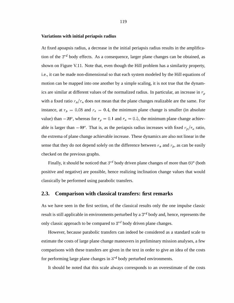
119

Variations with initial periapsis radius

At fixed apoapsis radius, a decrease in the initial periapsis radius results in the amplifica-

tion of the body effects. As a consequence, larger plane changes can be obtained, as

shown on Figure V.11. Note that, even though the Hill problem has a similarity property,

i.e., it can be made non-dimensional so that each system modeled by the Hill equations of

motion can be mapped into one another by a simple scaling, it is not true that the dynam-

ics are similar at different values of the normalized radius. In particular, an increase in with a fixed ratio does not mean that the plane changes realizable are the same. For

instance, at and , the minimum plane change is smaller (in absolute

value) than ! , whereas for and , the minimum plane change achiev-

able is larger than ! . That is, as the periapsis radius increases with fixed ratio,

the extrema of plane change achievable increase. These dynamics are also not linear in the

sense that they do not depend solely on the difference between and , as can be easily

checked on the previous graphs.

Finally, it should be noticed that body driven plane changes of more than ! (both

positive and negative) are possible, hence realizing inclination change values that would

classically be performed using parabolic transfers.

2.3. Comparison with classical transfers: first remarks

As we have seen in the first section, of the classical results only the one impulse classic

result is still applicable in environments perturbed by a body and, hence, represents the

only classic approach to be compared to body driven plane changes.

However, because parabolic transfers can indeed be considered as a standard scale to

estimate the costs of large plane change maneuvers in preliminary mission analyses, a few

comparisons with these transfers are given in the text in order to give an idea of the costs

for performing large plane changes in body perturbed environments.

It should be noted that this scale always corresponds to an overestimate of the costs

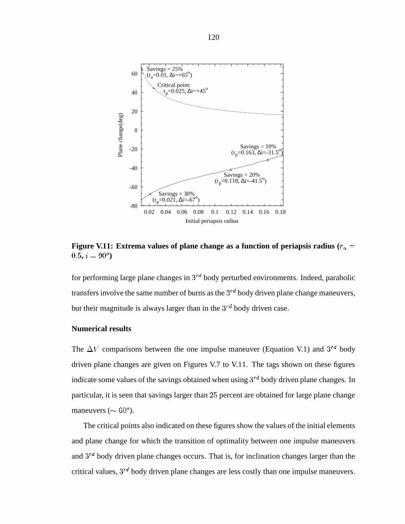
120

-80

-60

-40

-20

0

20

40

60

0.02 0.04 0.06 0.08 0.1 0.12 0.14 0.16 0.18

Plan

e ch

ange

(deg

)

Initial periapsis radius

*Critical point: rp=0.025, ∆i=+45o

x Savings = 25%(ra=0.01, ∆i=+65o)

x Savings = 30%(rp=0.021, ∆i=-67o)

x Savings = 20%(rp=0.118, ∆i=-41.5o)

x

Savings = 10%(rp=0.163, ∆i=-31.5o)

Figure V.11: Extrema values of plane change as a function of periapsis radius ( , ! )

for performing large plane changes in body perturbed environments. Indeed, parabolic

transfers involve the same number of burns as the body driven plane change maneuvers,

but their magnitude is always larger than in the body driven case.

Numerical results

The comparisons between the one impulse maneuver (Equation V.1) and body

driven plane changes are given on Figures V.7 to V.11. The tags shown on these figures

indicate some values of the savings obtained when using body driven plane changes. In

particular, it is seen that savings larger than percent are obtained for large plane change

maneuvers ( ! ).

The critical points also indicated on these figures show the values of the initial elements

and plane change for which the transition of optimality between one impulse maneuvers

and body driven plane changes occurs. That is, for inclination changes larger than the

critical values, body driven plane changes are less costly than one impulse maneuvers.

121

These critical plane change values depend on the initial conditions of the low altitude,

circular orbit ( , and ) and seem to increase (in absolute value) as the periapsis radius

decreases. For periapsis on the order of the normalized radius of Europa, the critical values

for optimality lie close to ! .As expected, for plane changes larger than ! , body driven maneuvers are less

costly than the classic scale of parabolic plane changes. The costs are lower by

in the case of Figure V.11 and more than in the case of Figure V.10. Also, we should

note the large savings made for the case of change of direction of motion (plane changes

of ! ), as shown on Figures V.8 and V.9. In this case, savings of more than are obtained when compared to the parabolic transfers and more than as compared

to 1-impulse plane changes. In addition, such transfers have the advantage of remaining

bounded, and in particular, the transfer time is much smaller than in the parabolic case.

All these results show that the classical optimality of bi-elliptic transfers over one im-

pulse maneuvers for plane changes larger than ! has an analogue in the case of body

perturbed environments, where bi-elliptic transfers are replaced by the body driven

plane changes defined here. This situation is, however, more complex than in the classical

case, since at any given initial conditions, the range of body driven plane changes re-

alizable is restricted. For example, the equatorial plane is invariant under the flow of the

Hill equations, and the only plane changes possible are ! or ! . One cannot transfer

a spacecraft from the equatorial plane to a polar orbit using only the natural dynamics,

whereas it is perfectly possible to do this using a one impulse maneuver. The next section

looks at this problem by using semi-analytical techniques.

3. Design problem and optimality

The aim of this section is to investigate the optimality of the body driven plane change

maneuvers presented above, by answering the question: given a spacecraft on a circular

orbit (with given radius and inclination ), what is the most cost effective approach to

122

perform a desired plane change maneuver ?While the analysis performed in the previous section searched for the global extrema

of plane changes that are realizable given some initial conditions [40], the answer to the

above question requires a closer look at the range of the possible plane changes realizable

using the body forces. This range does not cover the set of all allowable plane changes,

and one impulse maneuvers must still sometimes be used. In the case of body driven

plane changes, analytical estimates and a numerical algorithm are proposed to compare

third body driven transfers and direct one impulse maneuvers. It is shown, in particular,

that third body driven plane changes are always optimal above a critical value ( ! )

that depends on the initial conditions. The resulting criterion for optimality allows us

to directly choose the optimal approach for a plane change maneuver, given some initial

conditions.

3.1. Approaches to the solution

A natural approach to solve the optimality problem is to compare the given by the

different methods to perform the given plane change, " . For one impulse maneuvers,

this value is determined by equation (V.1) and for third body driven plane changes, one

needs to solve the following optimization problem:

subject to " and

(V.7)

Even though such an approach gives a complete solution to the problem, it is not

computationally effective and problem (V.7) does not have necessarily a solution for any

initial conditions.

Therefore, a better approach consists of first investigating the question of the optimal

method to be used without concern for the precise numerical value of the required. In

particular, a first computation must answer the question of the range of third body driven

plane changes that are possible. This is discussed in the next subsection by finding the

123

‘local-global’ extrema of .The Jacobi constant can be used to obtain rather sharp estimates for the body driven

needed to perform a given plane change with given initial conditions , , and .These estimates result in an upper bound (depending on , , and ) above which body driven plane changes are shown to be optimal.

However, these constraints do not solve the problem completely and a numerical algo-

rithm must be used to complete the answer. The idea of the algorithm proposed is based

on comparing the plane changes obtained via both methods for a given . This results

in reducing the question of the optimal method to solving problem (V.5) instead of (V.7).

3.2. Dynamical restriction on realizable transfers

In the previous section, the solution of (V.5) was solved by finding the global extrema

of on the manifolds . While there is a unique global

maximum and minimum for any given value of , and , their positions in the -space may not be on the same connected component of

. In such cases, it may happen

that the range of body driven plane changes between the computed extrema may not

be connected. This does happen in practice, especially for near equatorial orbits ( near !or ! ).

In order to determine the range of possible third body driven plane changes, the ex-

trema of are computed by pairs on each connected component of

. Any plane change

can then be realized between the two extrema of a given pair.

The connected components of

can be computed by first searching along the axis

and and then, by tracking the lines step by step along their

tangents, as in the previous section. Figure V.12 represents an example of manifold

with three different connected components with the location of the pair of extrema on

these components. In the case shown, the global extrema of plane change are located on

the same component and all plane change values between " and # ! are possible.

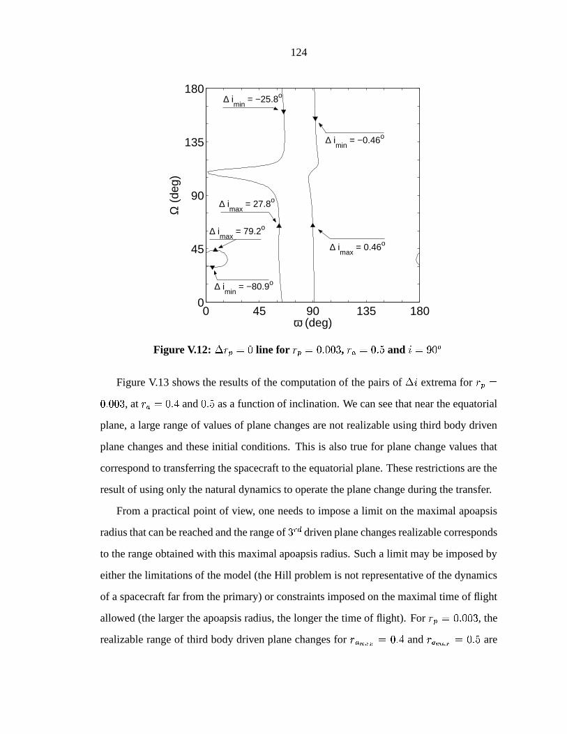
124

0 45 90 135 1800

45

90

135

180

∆ imin

= −80.9o

∆ imax

= 79.2o

∆ imin

= −25.8o

∆ imax

= 27.8o

∆ imin

= −0.46o

∆ imax

= 0.46o

ω (deg)

Ω (

deg)

Figure V.12: line for , " and !

Figure V.13 shows the results of the computation of the pairs of extrema for , at

and as a function of inclination. We can see that near the equatorial

plane, a large range of values of plane changes are not realizable using third body driven

plane changes and these initial conditions. This is also true for plane change values that

correspond to transferring the spacecraft to the equatorial plane. These restrictions are the

result of using only the natural dynamics to operate the plane change during the transfer.

From a practical point of view, one needs to impose a limit on the maximal apoapsis

radius that can be reached and the range of driven plane changes realizable corresponds

to the range obtained with this maximal apoapsis radius. Such a limit may be imposed by

either the limitations of the model (the Hill problem is not representative of the dynamics

of a spacecraft far from the primary) or constraints imposed on the maximal time of flight

allowed (the larger the apoapsis radius, the longer the time of flight). For , the

realizable range of third body driven plane changes for

and are

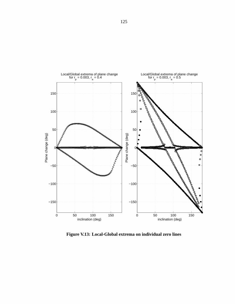
125

0 50 100 150

−150

−100

−50

0

50

100

150

inclination (deg)

Pla

ne c

hang

e (d

eg)

Local/Global extrema of plane change for r

p = 0.003, r

a = 0.4

0 50 100 150

−150

−100

−50

0

50

100

150

inclination (deg)

Pla

ne c

hang

e (d

eg)

Local/Global extrema of plane change for r

p = 0.003, r

a = 0.5

Figure V.13: Local-Global extrema on individual zero lines

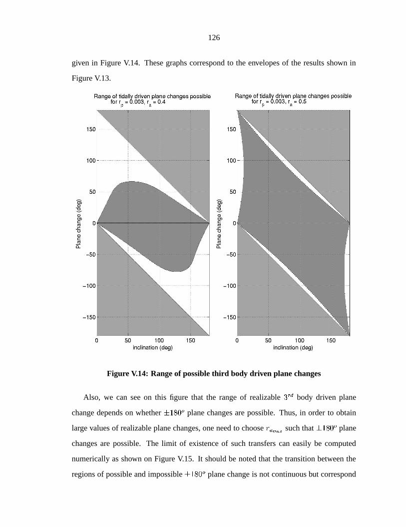
126

given in Figure V.14. These graphs correspond to the envelopes of the results shown in

Figure V.13.

Figure V.14: Range of possible third body driven plane changes

Also, we can see on this figure that the range of realizable body driven plane

change depends on whether ! plane changes are possible. Thus, in order to obtain

large values of realizable plane changes, one need to choose such that ! plane

changes are possible. The limit of existence of such transfers can easily be computed

numerically as shown on Figure V.15. It should be noted that the transition between the

regions of possible and impossible ! plane change is not continuous but correspond

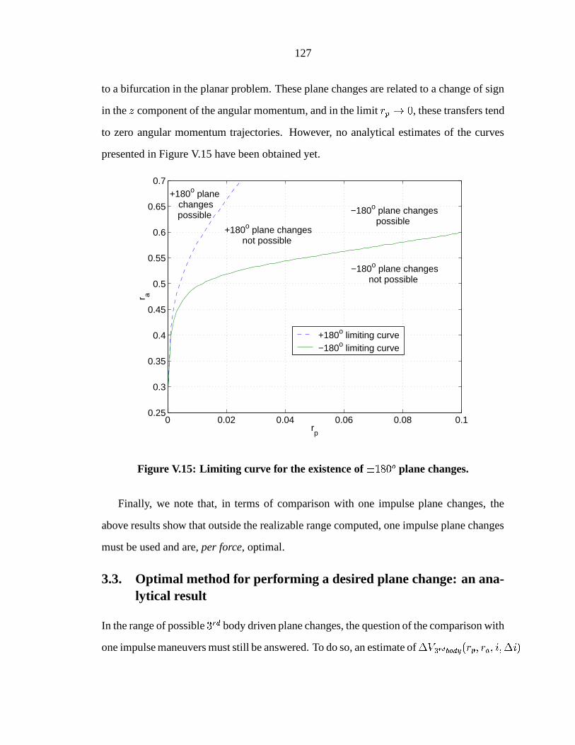
127

to a bifurcation in the planar problem. These plane changes are related to a change of sign

in the component of the angular momentum, and in the limit , these transfers tend

to zero angular momentum trajectories. However, no analytical estimates of the curves

presented in Figure V.15 have been obtained yet.

0 0.02 0.04 0.06 0.08 0.10.25

0.3

0.35

0.4

0.45

0.5

0.55

0.6

0.65

0.7

rp

r a

+180o limiting curve−180o limiting curve

+180o plane changespossible −180o plane changes

possible +180o plane changes

not possible

−180o plane changesnot possible

Figure V.15: Limiting curve for the existence of ! plane changes.

Finally, we note that, in terms of comparison with one impulse plane changes, the

above results show that outside the realizable range computed, one impulse plane changes

must be used and are, per force, optimal.

3.3. Optimal method for performing a desired plane change: an ana-lytical result

In the range of possible body driven plane changes, the question of the comparison with

one impulse maneuvers must still be answered. To do so, an estimate of !

128

is obtained first, via the Jacobi constant expressed in inertial coordinates:

#

(V.8)

where , and denote, respectively, the magnitude of the position, velocity and angular

momentum vector in inertial space (same origin as in the rotating frame).

Along a transfer trajectory, and

have been chosen so that . It follows that

the terms depending only on cancel out in the difference of the Jacobi constant taken

between the final and initial periapsis passages of the transfer trajectory. Moreover, at

periapsis, the angular momentum magnitude is expressed as so that we obtain:

# #

(V.9)

where the subscripts and refer to the initial and final periapsis, respectively.

Now, denoting , we can solve for (quadratic form in ):

# #

# # # (V.10)

Note, here, that is expressed in terms of and of the transfer trajectory at the initial

periapsis as where only depends on the ratio .

is the local circular speed in inertial space.

The quantity in (V.10) depends on and

and can be bounded as # , so that we obtain a bound on as:

(V.11)

where

# #

# #

# #

# #

It results that ! # is also bounded, ! , yielding a bound on the limit of optimality for one impulse plane

change maneuvers. Indeed, for any in the realizable range, the minimum ! to

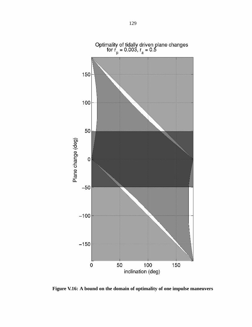
129

Figure V.16: A bound on the domain of optimality of one impulse maneuvers

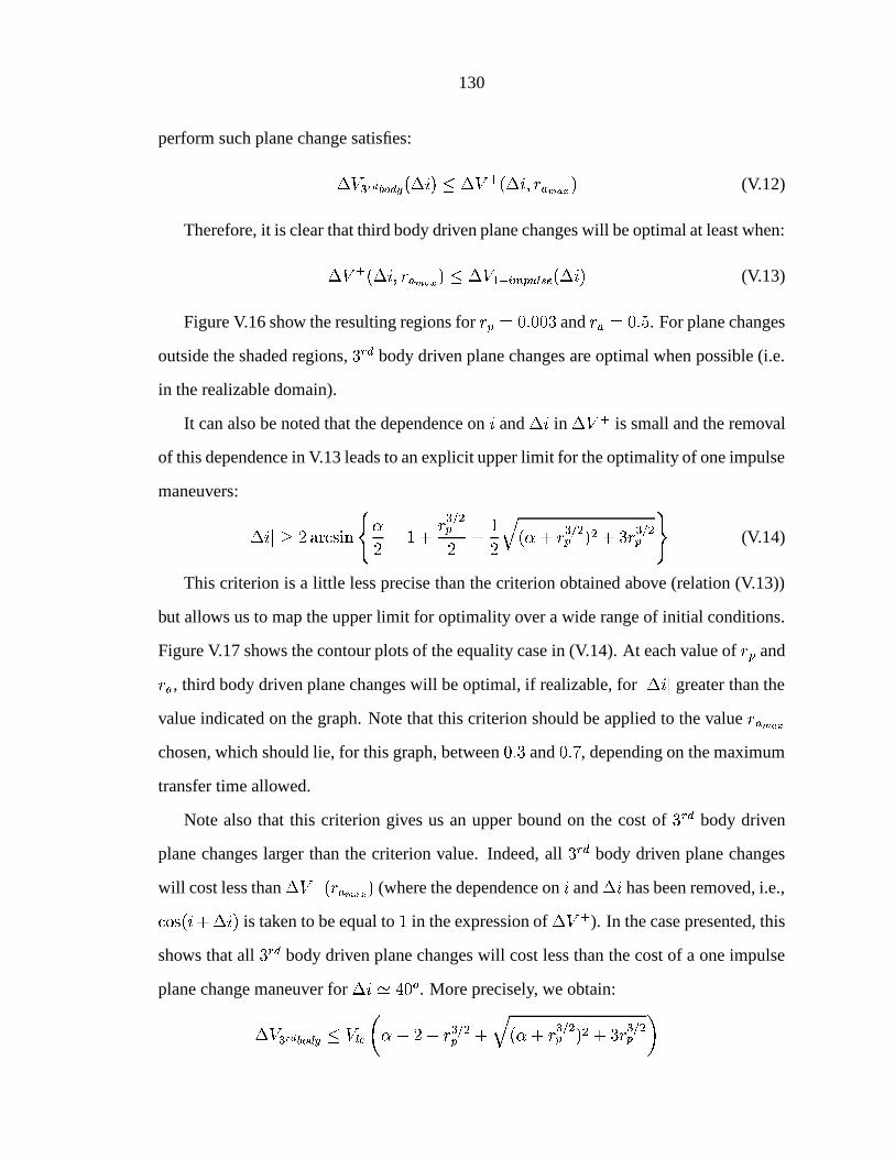
130

perform such plane change satisfies:

! (V.12)

Therefore, it is clear that third body driven plane changes will be optimal at least when:

(V.13)

Figure V.16 show the resulting regions for and " . For plane changes

outside the shaded regions, body driven plane changes are optimal when possible (i.e.

in the realizable domain).

It can also be noted that the dependence on and in is small and the removal

of this dependence in V.13 leads to an explicit upper limit for the optimality of one impulse

maneuvers:

#

#

# #

(V.14)

This criterion is a little less precise than the criterion obtained above (relation (V.13))

but allows us to map the upper limit for optimality over a wide range of initial conditions.

Figure V.17 shows the contour plots of the equality case in (V.14). At each value of and

, third body driven plane changes will be optimal, if realizable, for greater than the

value indicated on the graph. Note that this criterion should be applied to the value

chosen, which should lie, for this graph, between and , depending on the maximum

transfer time allowed.

Note also that this criterion gives us an upper bound on the cost of body driven

plane changes larger than the criterion value. Indeed, all body driven plane changes

will cost less than (where the dependence on and has been removed, i.e.,

# is taken to be equal to in the expression of ). In the case presented, this

shows that all body driven plane changes will cost less than the cost of a one impulse

plane change maneuver for ! . More precisely, we obtain:

! # # # #

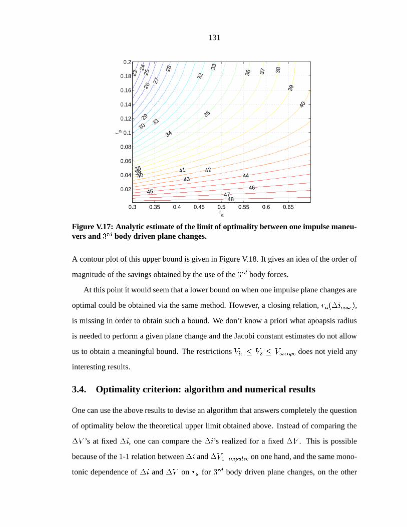
131

0.3 0.35 0.4 0.45 0.5 0.55 0.6 0.65

0.02

0.04

0.06

0.08

0.1

0.12

0.14

0.16

0.18

0.2

ra

r p

2324

2526

27

28

29

30 31

32

33

34

35

36 37 38

38

39

3940

40

41 42

43 44

4546

4748

Figure V.17: Analytic estimate of the limit of optimality between one impulse maneu-vers and body driven plane changes.

A contour plot of this upper bound is given in Figure V.18. It gives an idea of the order of

magnitude of the savings obtained by the use of the body forces.

At this point it would seem that a lower bound on when one impulse plane changes are

optimal could be obtained via the same method. However, a closing relation, ,is missing in order to obtain such a bound. We don’t know a priori what apoapsis radius

is needed to perform a given plane change and the Jacobi constant estimates do not allow

us to obtain a meaningful bound. The restrictions does not yield any

interesting results.

3.4. Optimality criterion: algorithm and numerical results

One can use the above results to devise an algorithm that answers completely the question

of optimality below the theoretical upper limit obtained above. Instead of comparing the

’s at fixed , one can compare the ’s realized for a fixed . This is possible

because of the 1-1 relation between and on one hand, and the same mono-

tonic dependence of and on for body driven plane changes, on the other

132

0.3 0.35 0.4 0.45 0.5 0.55 0.6 0.65

0.02

0.04

0.06

0.08

0.1

0.12

0.14

0.16

0.18

0.2

ra

r p

1

1.2

1.4

1.6

1.8 2

2.32.6

3

4

56

8 1015 20

Figure V.18: Analytic upper bound for the cost of body driven plane changes.

hand.

Given " , we have given by equation (V.1). Then we can solve for in

, yielding two solutions :

(V.15)

where

# # # #

Now, problem V.5 can be solved numerically with , resulting in to be compared

with " . However, note that, when " , one needs to solve exactly for

! to decide of the optimality by comparing with . In practice, this

case covers only a very thin strip of initial conditions and generally, the above algorithm

requires only solving problem (V.5) once or twice per initial conditions to settle the ques-

tion.

Numerical computations for the case shown in Figure V.16 shows that the theoretical

limit (V.13) is within ! of the numerically computed limit.

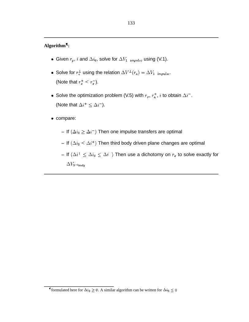
133

Algorithm :

Given , and " , solve for using (V.1).

Solve for using the relation .(Note that ).

Solve the optimization problem (V.5) with , , to obtain .

(Note that ).

compare:

– If " Then one impulse transfers are optimal

– If " Then third body driven plane changes are optimal

– If " Then use a dichotomy on to solve exactly for

!

formulated here for $ . A similar algorithm can be written for $

CHAPTER VI

ESCAPE, CAPTURE AND TRANSIT

This chapter presents a second application of the use of body forces to effect orbital

transfers. As for the previous application, this second application, escape and capture

maneuvers, was also motivated by the Europa Orbiter Mission.

While the transfers considered are analyzed using a periapsis Poincaré map, the initial

conditions are chosen on a surface of section close to the libration points and the map is

then obtained by backward integration. The main difference between the previous chapters

(IV and V) is that the existence of a next (or previous) periapsis passage is not guaranteed

(since we are working at energies where the zero velocity surface is open, i.e., ).

Thus, this approach shows the limits of the approximations of the periapsis Poincaré maps

obtained in Chapter IV.

Note that, unlike body driven plane changes, low energy transit trajectories have

been studied by several authors, the first one being Conley [9], who analyzed the flow

near the collinear libration points in the planar circular restricted three body problem

(PCR3BP). Belbruno [4] pointed out that these nonlinear dynamics can be used to nu-

merically compute ballistic transfers to the moon and gave several ways of finding such

transfers. More recent work by Koon et al. [21, 20] gives a more rigorous explanation of

these phenomena by applying some techniques from dynamical systems theory to systems

of coupled PCR3BP. They obtained a systematic way of designing ballistic lunar transfers

and, more generally, trajectories with a predetermined future and past (in terms of transfer

from the inner side of the orbit of the primary to the outer side).

134

135

In this chapter, we give another view of the geometry of escaping trajectories, focusing

on obtaining practical characterizations of the initial conditions of these escaping trajec-

tories at periapsis. Applications of these results are made to the analysis of direct escape

maneuvers. In particular, the minimum energy needed to directly escape, starting at a given

altitude, is obtained. These results should be useful for mission design and planning.

While the results presented here were first reported in [38], this chapter takes a slightly

different point of view by relating these results to the linearized theory at the libration

points and the notion of escaping trajectory is slightly sharpened. In [38], escape has been

considered from a practical viewpoint where any trajectories crossing the plane with an outward velocity (with respect to the primary) was considered to be an escaping

trajectory. The aim of the paper was indeed to obtain estimates of the initial costs for

escape starting in a low altitude, circular orbit (thus close to the primary) and once near

the libration points, a very small may be used to transfer the spacecraft on a trajectory

that will never meet the planetary satellite again.

In this chapter, the set of escaping trajectories that come close to the primary are in-

tegrated forward to check that they indeed correspond to escaping trajectories for the Hill

problem and can be patched onto the outer restricted three body problem if needed. This

does not mean, however, that the spacecraft will not meet the planetary satellite in the

framework of the restricted three body problem, but the time of return will at least be

much larger than the period of the primary around the disturbing body.

In Section , we review the dynamics near the libration points, following a paper by

Conley [9], resulting in a classification of the trajectories in this region. The use of a

periapsis Poincaré map allows us to extend this local picture up to the neighborhood of

the primary by integrating the flow backward, resulting also in a proposed classification of

planetary satellites.

Applications of the previous results are then made, in Section , to the problem of

directly escaping trajectories assuming a spacecraft initially in a low altitude, circular orbit.

136

It is shown, in particular, that the minimum to directly escape is obtained for tangential

burns and that this minimum decreases as altitude increases. A new optimality criterion

is then stated for the class of directly escaping trajectories using one impulsive maneuver,

resulting in fuel savings on the order of 130 m/s in the case of Europa (as compared to

a two body Keplerian model). Given an initial altitude, the optimal Jacobi constant and

the minimum required to reach escape can be read from some graphs. The time of

the maneuver is determined by a condition on the longitude of the ascending node and the

argument of periapsis of the transfer trajectory, similar to the previous chapter. Restrictions

on the inclination for these transfers to be possible also exist, as the initial orbit must be

near-equatorial.

1. Periapsis Poincaré map for escape, capture and transit

We have seen in Chapter III that the linearized dynamics at the libration points is given by

a -dimensional center manifold and two -dimensional invariant manifolds (one stable

and one unstable direction) in the planar case. In the spatial problem, the center manifold

is-dimensional and consists of periodic and quasi-periodic trajectories. This section

presents a closer look at these dynamics by first recalling some results from [9] and then

extending the local picture obtained with the help of numerical integration methods. The

consequences of the results obtained are discussed.

1.1. Taxonomy of trajectories near the libration points

Recall from chapter III that the linearized dynamics around the libration points is given

by:

;

;

and the eigenvalues are denoted

, and , where:

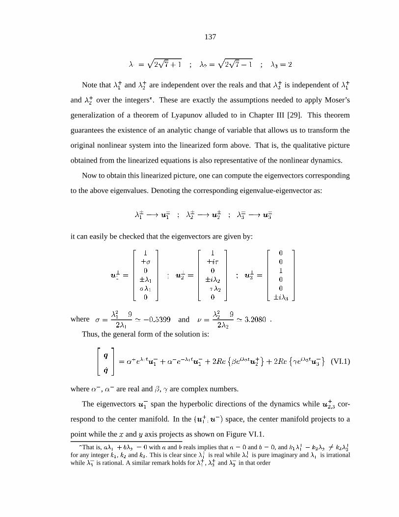
137

# ;

;

Note that and

are independent over the reals and that

is independent of

and over the integers . These are exactly the assumptions needed to apply Moser’s

generalization of a theorem of Lyapunov alluded to in Chapter III [29]. This theorem

guarantees the existence of an analytic change of variable that allows us to transform the

original nonlinear system into the linearized form above. That is, the qualitative picture

obtained from the linearized equations is also representative of the nonlinear dynamics.

Now to obtain this linearized picture, one can compute the eigenvectors corresponding

to the above eigenvalues. Denoting the corresponding eigenvalue-eigenvector as:

it can easily be checked that the eigenvectors are given by:

where

and

.

Thus, the general form of the solution is:

# # # (VI.1)

where

, are real and

, are complex numbers.

The eigenvectors span the hyperbolic directions of the dynamics while cor-

respond to the center manifold. In the space, the center manifold projects to a

point while the and axis projects as shown on Figure VI.1.That is, ! $ with and reals implies that $ and $ , and ! ! ' '

for any integer , ! and ' . This is clear since is real while ! is pure imaginary and is irrationalwhile ' is rational. A similar remark holds for , ' and ! in that order

138

u1-

x

y

u1+

Transit

Transit

Non-transit

Non-transit

Figure VI.1: Stable and unstable direction of the libration points dynamics

Thus, when,

, the trajectories cross the axis and go from to # (or

vice versa) in this linearized setting. If , the trajectories stay on one side of the

the -axis.Thus Conley [9] proposed the following classification:

: transit trajectories

: non-transit trajectories

: asymptotic trajectories

where the last class includes the center manifold as well. This classification was originally

derived in the restricted three body problem where transit trajectories go from one region

dominated by the gravitational attraction of one body to a region dominated by the second

body. In our case, transit trajectories are either escaping trajectories when going from the

inner region to the outer region of the Hill’s problem, or capture trajectories when going

the other way.

Note that it can easily be proven in this linear setting that non-escaping trajectories are

bounded by the lines that are tangent to the Lyapunov orbits at their apses. That is, non-

transit trajectories coming from the inner region cannot go further than the planes

tangent to the apoapsis of the Lyapunov orbits. Thus, as far as this linear picture holds,

139

if an integrated trajectory crosses the neck from one side of a Lyapunov orbit to the other

side (as defined by the above tangent planes), then the trajectory is a transit trajectory.

From a practical point of view, we will integrate the trajectories up to a radius to

check escape.

At a given value of , it can also be shown from (VI.1), that the envelope of the transit

trajectories consists of the set of asymptotic trajectories. This set forms, moreover, a ‘tube’

that separates the phase space. In the planar problem, these tubes project onto some strips

(resp., solid cylinders in the spatial problem) in position space and any initial condition

outside these tubes corresponds to a non-transit trajectory, no matter what the direction of

the velocity is. Inside the strips, transit and non-transit trajectories are distinguished by a

condition on the velocity direction.

In the case of escaping trajectories at , the tubes are formed by the inner branch of

the stable manifold associated with the center manifold, , and the outer branch of the

unstable manifold, . Llibre et al. [22] have shown that for low values of (i.e., such

that the above linear picture holds), extends to infinity in the planar Hill problem. That

is, in the framework of the Hill problem, once an escape trajectory crossed the neck region,

it never comes back close to the primary, i.e., it is really an escape trajectory. However, in

the framework of the restricted problem, the spacecraft can return close to the neck region

after one or several loops around the disturbing body and encounter the primary again.

In view of these results, a trajectory can be considered as escaping as soon as it crosses

the neck region and numerical integration only needs to be performed up to that point.

However, since an estimate of the value of the Jacobi constant for which the linear picture

can be used is not available, we will numerically integrate escaping trajectories up to

to ensure escape.

Concerning capture trajectories, we defined them as trajectories that come from the

outer regions, cross one of the neck and then have at least one of their periapsis passages

close to the primary (i.e. inside the first curve of chapter IV). Thus, in view

140

of the symmetry of the Hill problem (time-reversal reflection about the -plane),

we see that the symmetric of an escape trajectory is a capture one and vice versa. It is

therefore sufficient to analyze escaping trajectories to obtain a complete characterization

of transit trajectories.

Finally, we should note that while the above picture has first been obtained by Conley

in the planar case

, the three dimensional case has been obtained by Appleyard [1] and a

more recent presentation is given in [11].

1.2. Numerical integration of escaping trajectories

In view of the preceding results, the envelope of the escaping trajectories can simply be

obtained by computing . This computation is, however, subtle and a more direct nu-

merical scheme is proposed to analyze escaping trajectories. This scheme is closely tied

with the results presented in [38] and consists of integrating the outward flow of the neck

regions close to the libration points, back to the previous periapsis passages . Because of

the symmetries and (see Chapter III), we only need to integrate the outward flow

near and at those points having a positive coordinate.

From the linearized results, it would seem that a good choice of surface of section in

the neck regions would be a sphere or plane, normal to the -axis and located just above

the apoapsis of the Lyapunov orbits (as viewed from the primary). This choice requires,

however, to compute the Lyapunov orbit and the precise value at which the surface must

be located is not clear for large values of . It should be taken far enough to ensure that

non-transit trajectories from the inside regions do not cross the surface, yet not too far

since the number of points used to integrate the flow increases with the area of the surfaceOne should be careful in reading Conley’s paper because of an error in the linearization (the matrix

should really be ). This error does not change the results except for a global reversal of time. Thus, thedirection of the Lyapunov orbit is clockwise and not counter-clockwise.

The ‘flow’ is integrated by randomly sampling the phase space region corresponding to the initial con-ditions and using an integration subroutine to propagate in time this discrete set of points. The difficultywith this approach lies in the large number of sampling points that may be required to obtained a sufficientaccuracy for computing, for exmaple, the boundary of the phase space region considered.

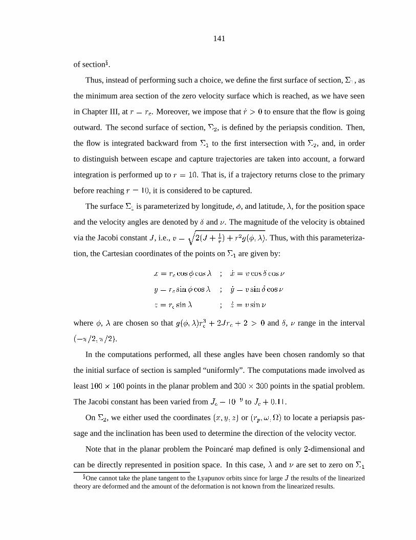
141

of section.

Thus, instead of performing such a choice, we define the first surface of section, , as

the minimum area section of the zero velocity surface which is reached, as we have seen

in Chapter III, at . Moreover, we impose that to ensure that the flow is going

outward. The second surface of section, , is defined by the periapsis condition. Then,

the flow is integrated backward from to the first intersection with , and, in order

to distinguish between escape and capture trajectories are taken into account, a forward

integration is performed up to . That is, if a trajectory returns close to the primary

before reaching , it is considered to be captured.

The surface is parameterized by longitude, , and latitude,

, for the position space

and the velocity angles are denoted by and . The magnitude of the velocity is obtained

via the Jacobi constant , i.e., #

# . Thus, with this parameteriza-

tion, the Cartesian coordinates of the points on are given by:

;

;

;

where ,

are chosen so that # # and , range in the interval

.In the computations performed, all these angles have been chosen randomly so that

the initial surface of section is sampled “uniformly”. The computations made involved as

least points in the planar problem and points in the spatial problem.

The Jacobi constant has been varied from #

to # .

On , we either used the coordinates or to locate a periapsis pas-

sage and the inclination has been used to determine the direction of the velocity vector.

Note that in the planar problem the Poincaré map defined is only -dimensional and

can be directly represented in position space. In this case,

and are set to zero on One cannot take the plane tangent to the Lyapunov orbits since for large the results of the linearized

theory are deformed and the amount of the deformation is not known from the linearized results.

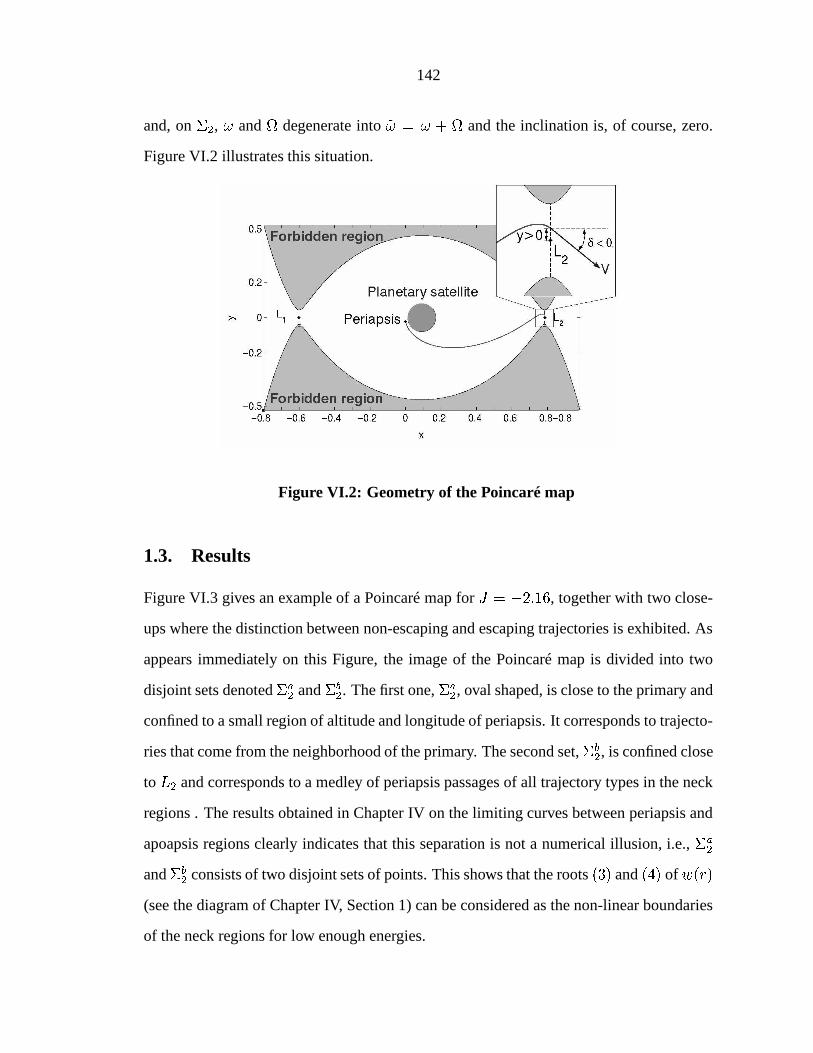
142

and, on , and

degenerate into # and the inclination is, of course, zero.

Figure VI.2 illustrates this situation.

Figure VI.2: Geometry of the Poincaré map

1.3. Results

Figure VI.3 gives an example of a Poincaré map for ! , together with two close-

ups where the distinction between non-escaping and escaping trajectories is exhibited. As

appears immediately on this Figure, the image of the Poincaré map is divided into two

disjoint sets denoted and

. The first one, , oval shaped, is close to the primary and

confined to a small region of altitude and longitude of periapsis. It corresponds to trajecto-

ries that come from the neighborhood of the primary. The second set,

, is confined close

to and corresponds to a medley of periapsis passages of all trajectory types in the neck

regions . The results obtained in Chapter IV on the limiting curves between periapsis and

apoapsis regions clearly indicates that this separation is not a numerical illusion, i.e., and

consists of two disjoint sets of points. This shows that the roots and of (see the diagram of Chapter IV, Section 1) can be considered as the non-linear boundaries

of the neck regions for low enough energies.

143

In the sequel, we will focus almost exclusively on the first region, . It is, indeed,

the most important set to be considered for the practical application of these computations

to the problem of direct escape from a planetary satellite. The main information coming

from the set

is a measure of the extent to which the neck region extends.

We can also see from Figure VI.3 that the non-escaping trajectories coming from the

vicinity of the primary surround the set of escaping trajectories, . From the linearized

results, we know that the boundary of should be the stable manifold associated with

the Lyapunov orbit at . As we can see, the set of non-escaping trajectories computed

(i.e., the non-escaping trajectories that reach with an outward velocity) is rather small

and the distance between this set and will decrease forward in time under the influence

of . Thus, in the neck region, a small will be sufficient to transfer a non-escaping

particle that cross onto an escaping trajectory, thus supporting the pragmatic viewpoint

adopted in [38].

The above remarks made for the planar Poincaré map shown in Figure VI.3 remain

valid for the results obtained in the spatial problem. It is found that the set of points

obtained is divided into two disjoint sets and

, whose intersections with the ( )-

plane match the image of the Poincaré map in the planar case. The three dimensional

picture of looks like the set of points obtained from the planar , by rotating it along

its diameter (the line connecting the points of extremal radius on this set). Restrictions on

inclination for are given in Figure VI.11 and will be discussed in the next section.

Note, however, that, unlike the planar case, the projection of the set of non-escaping

points onto position space includes all the points in the projection of . Indeed, is

four dimensional in the spatial problem and the separation between escape and non-escape

also involves the inclination of the velocity vector. Thus, at a given position, small values

of inclination may correspond to a escaping trajectory, while larger values will correspond

to non-escaping trajectories.

As varies, the size and shape of varies. Figure VI.4 shows a series of Poincaré

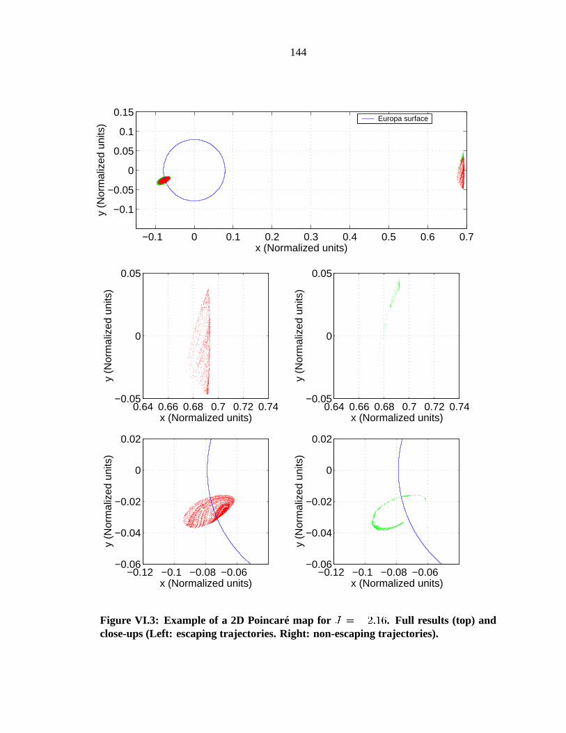
144

−0.1 0 0.1 0.2 0.3 0.4 0.5 0.6 0.7

−0.1

−0.05

0

0.05

0.1

0.15

x (Normalized units)

y (N

orm

aliz

ed u

nits

)

Europa surface

0.64 0.66 0.68 0.7 0.72 0.74−0.05

0

0.05


y (N

orm

aliz

ed u

nits

)

0.64 0.66 0.68 0.7 0.72 0.74−0.05

0

0.05


y (N

orm

aliz

ed u

nits

)

−0.12 −0.1 −0.08 −0.06−0.06

−0.04

−0.02

0

0.02


y (N

orm

aliz

ed u

nits

)

−0.12 −0.1 −0.08 −0.06−0.06

−0.04

−0.02

0

0.02


y (N

orm

aliz

ed u

nits

)

Figure VI.3: Example of a 2D Poincaré map for . Full results (top) andclose-ups (Left: escaping trajectories. Right: non-escaping trajectories).

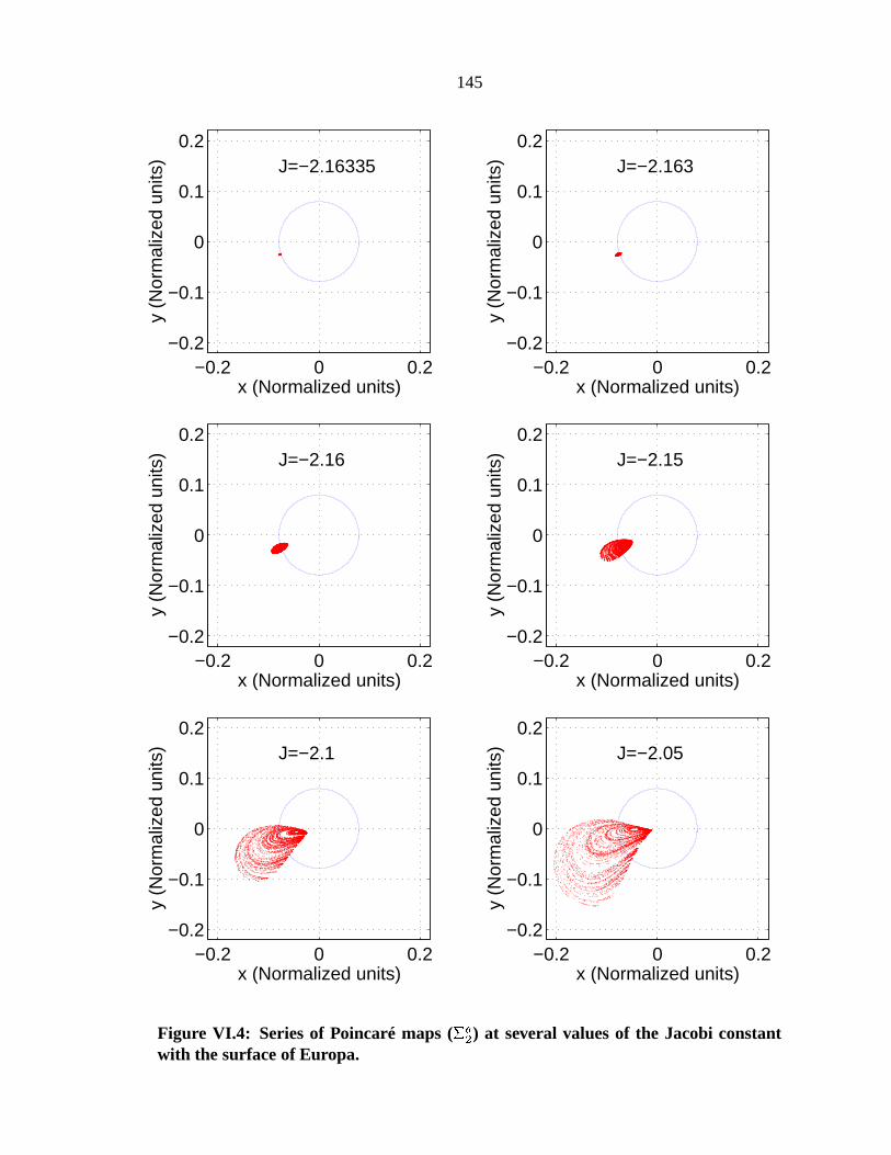
145

−0.2 0 0.2−0.2

−0.1

0

0.1

0.2


y (N

orm

aliz

ed u

nits

) J=−2.16335

−0.2 0 0.2−0.2

−0.1

0

0.1

0.2


y (N

orm

aliz

ed u

nits

) J=−2.163

−0.2 0 0.2−0.2

−0.1

0

0.1

0.2


y (N

orm

aliz

ed u

nits

) J=−2.16

−0.2 0 0.2−0.2

−0.1

0

0.1

0.2


y (N

orm

aliz

ed u

nits

) J=−2.15

−0.2 0 0.2−0.2

−0.1

0

0.1

0.2


y (N

orm

aliz

ed u

nits

) J=−2.1

−0.2 0 0.2−0.2

−0.1

0

0.1

0.2


y (N

orm

aliz

ed u

nits

) J=−2.05

Figure VI.4: Series of Poincaré maps ( ) at several values of the Jacobi constantwith the surface of Europa.

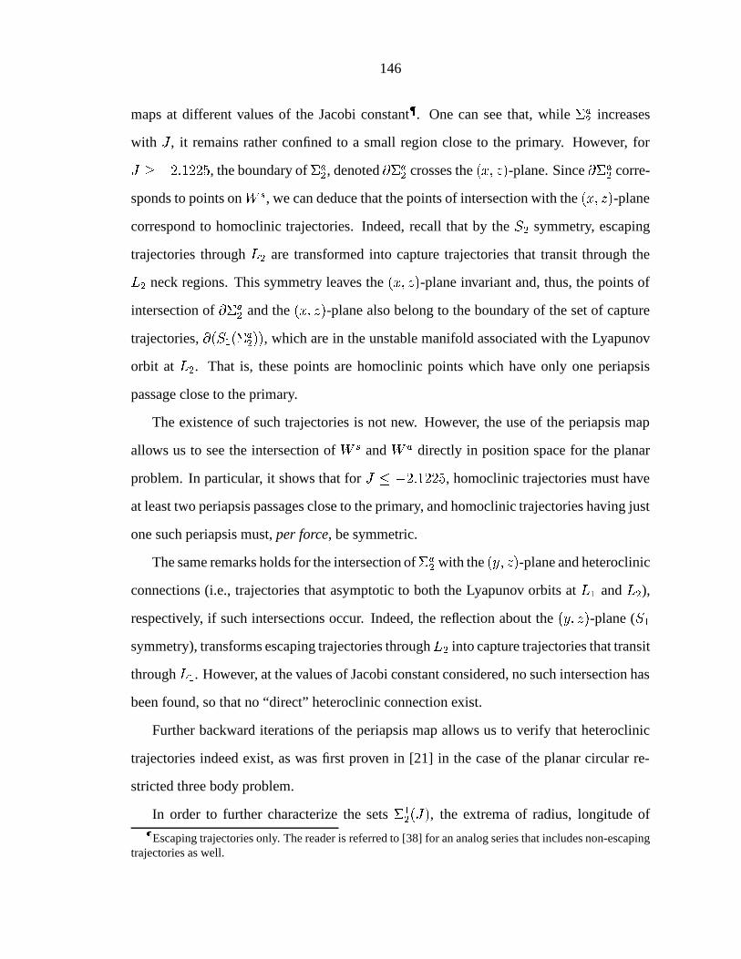
146

maps at different values of the Jacobi constant . One can see that, while increases

with , it remains rather confined to a small region close to the primary. However, for

! , the boundary of , denoted crosses the -plane. Since

corre-

sponds to points on , we can deduce that the points of intersection with the -plane

correspond to homoclinic trajectories. Indeed, recall that by the symmetry, escaping

trajectories through are transformed into capture trajectories that transit through the

neck regions. This symmetry leaves the -plane invariant and, thus, the points of

intersection of and the -plane also belong to the boundary of the set of capture

trajectories, , which are in the unstable manifold associated with the Lyapunov

orbit at . That is, these points are homoclinic points which have only one periapsis

passage close to the primary.

The existence of such trajectories is not new. However, the use of the periapsis map

allows us to see the intersection of and directly in position space for the planar

problem. In particular, it shows that for , homoclinic trajectories must have

at least two periapsis passages close to the primary, and homoclinic trajectories having just

one such periapsis must, per force, be symmetric.

The same remarks holds for the intersection of with the -plane and heteroclinic

connections (i.e., trajectories that asymptotic to both the Lyapunov orbits at and ),

respectively, if such intersections occur. Indeed, the reflection about the -plane ( symmetry), transforms escaping trajectories through into capture trajectories that transit

through . However, at the values of Jacobi constant considered, no such intersection has

been found, so that no “direct” heteroclinic connection exist.

Further backward iterations of the periapsis map allows us to verify that heteroclinic

trajectories indeed exist, as was first proven in [21] in the case of the planar circular re-

stricted three body problem.

In order to further characterize the sets , the extrema of radius, longitude ofEscaping trajectories only. The reader is referred to [38] for an analog series that includes non-escaping

trajectories as well.

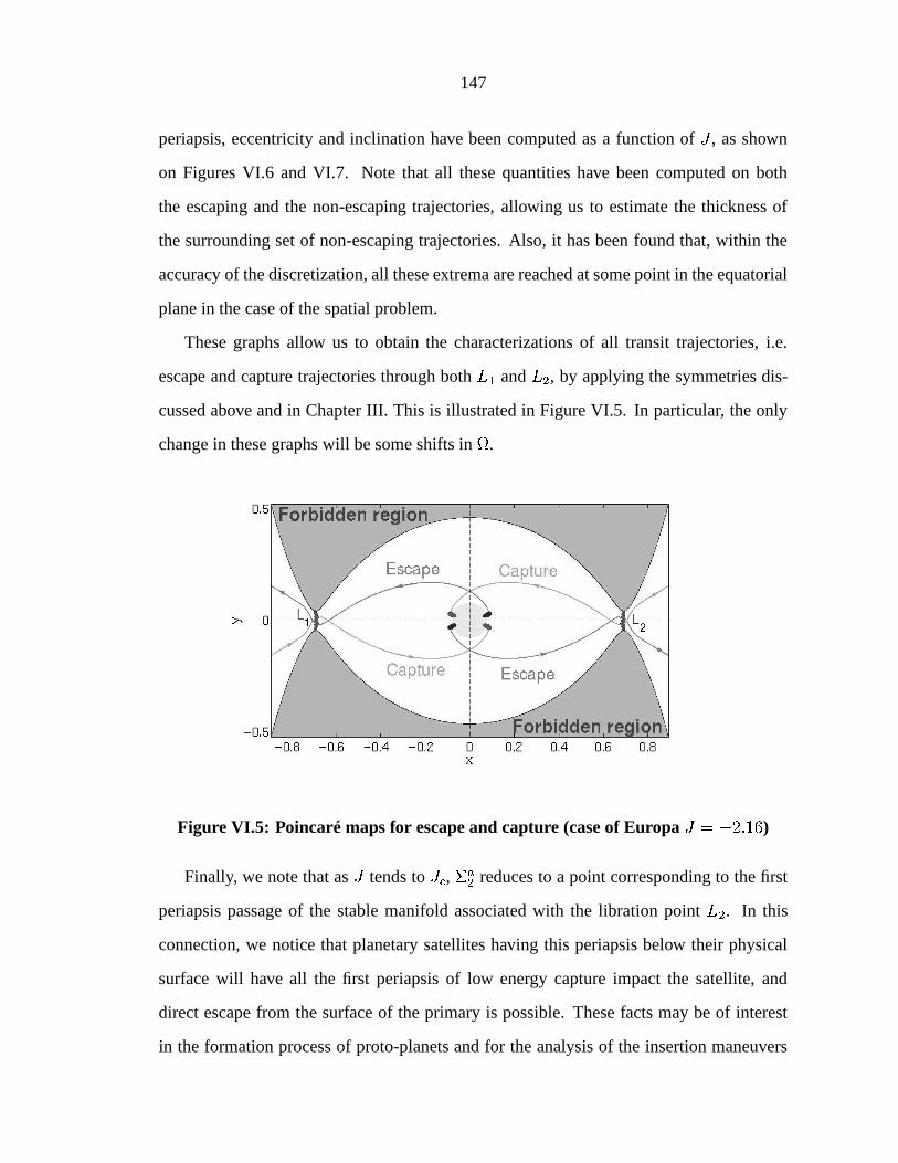
147

periapsis, eccentricity and inclination have been computed as a function of , as shown

on Figures VI.6 and VI.7. Note that all these quantities have been computed on both

the escaping and the non-escaping trajectories, allowing us to estimate the thickness of

the surrounding set of non-escaping trajectories. Also, it has been found that, within the

accuracy of the discretization, all these extrema are reached at some point in the equatorial

plane in the case of the spatial problem.

These graphs allow us to obtain the characterizations of all transit trajectories, i.e.

escape and capture trajectories through both and , by applying the symmetries dis-

cussed above and in Chapter III. This is illustrated in Figure VI.5. In particular, the only

change in these graphs will be some shifts in

.

Figure VI.5: Poincaré maps for escape and capture (case of Europa )

Finally, we note that as tends to , reduces to a point corresponding to the first

periapsis passage of the stable manifold associated with the libration point . In this

connection, we notice that planetary satellites having this periapsis below their physical

surface will have all the first periapsis of low energy capture impact the satellite, and

direct escape from the surface of the primary is possible. These facts may be of interest

in the formation process of proto-planets and for the analysis of the insertion maneuvers

148

of spacecraft around these satellites. In particular, this shows that very low energy capture

trajectories are not viable options for insertion around these celestial bodies and low energy

capture maneuvers would have to be designed carefully (since at any value of a large set

of capture trajectories will impact). In [38], we proposed to refer such planetary satellites

as being of type , the other planetary satellites being referred to as type (i.e., having the

periapsis of the stable manifold associated with above their physical surface. Table

1 in Appendix B gives the type of many planetary satellites in the solar system. For

example, Miranda is of type 1 (periapsis below the surface), Europa, Titan and Triton are

of type 2 (periapsis above the surface). Note however, that Europa is rather exceptional:

the periapsis of the stable (and unstable) manifold associated with (or ) lies only above the surface of Europa .

Periapsis radius of the stable manifold $ $ $ . Normalized radius of Europa %$ $ .

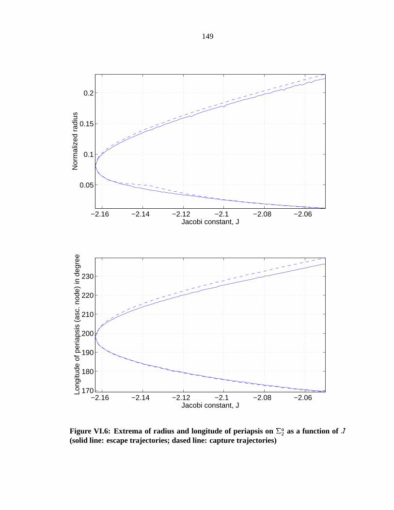
149

−2.16 −2.14 −2.12 −2.1 −2.08 −2.06

0.05

0.1

0.15

0.2

Jacobi constant, J

Nor

mal

ized

rad

ius

−2.16 −2.14 −2.12 −2.1 −2.08 −2.06170

180

190

200

210

220

230

Jacobi constant, J

Long

itude

of p

eria

psis

(as

c. n

ode)

in d

egre

e

Figure VI.6: Extrema of radius and longitude of periapsis on as a function of (solid line: escape trajectories; dased line: capture trajectories)

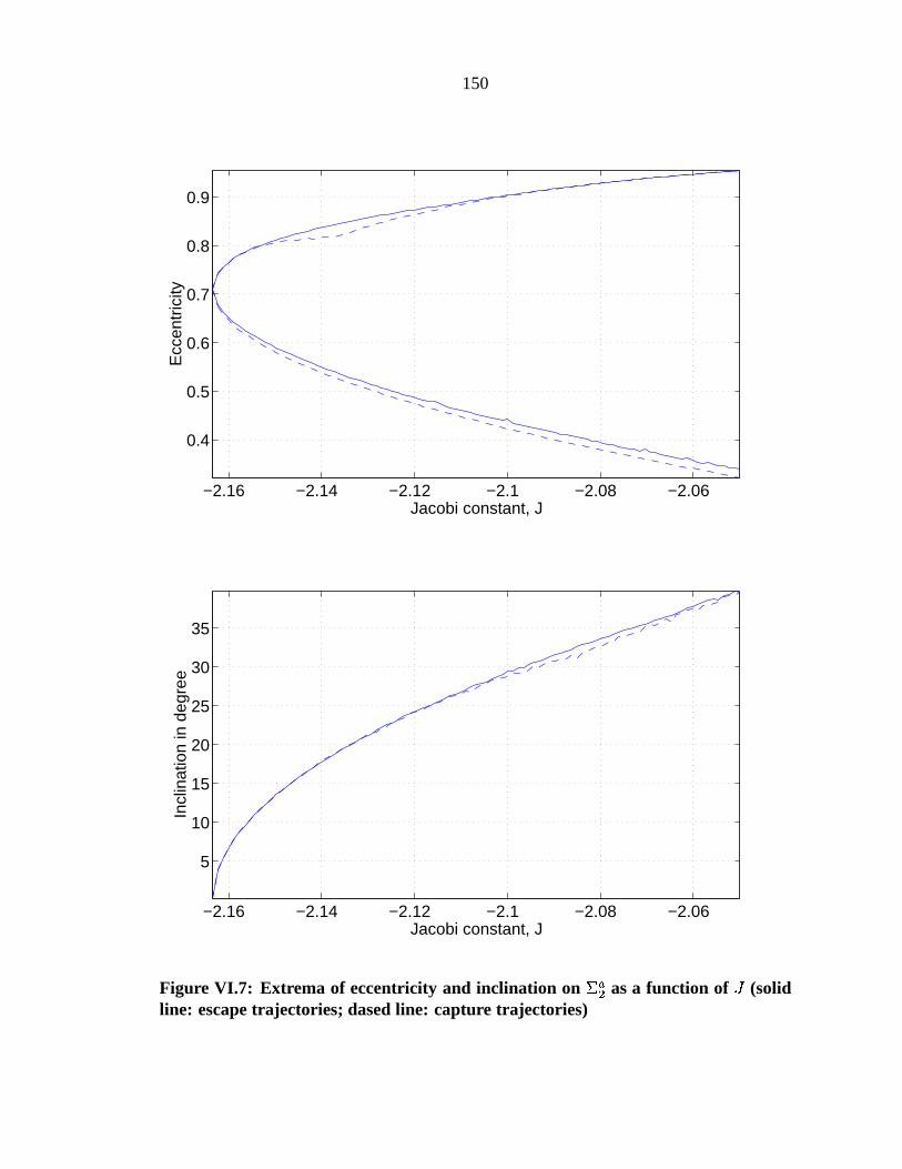
150

−2.16 −2.14 −2.12 −2.1 −2.08 −2.06

0.4

0.5

0.6

0.7

0.8

0.9

Jacobi constant, J

Ecc

entr

icity

−2.16 −2.14 −2.12 −2.1 −2.08 −2.06

5

10

15

20

25

30

35

Jacobi constant, J

Incl

inat

ion

in d

egre

e

Figure VI.7: Extrema of eccentricity and inclination on as a function of (solidline: escape trajectories; dased line: capture trajectories)

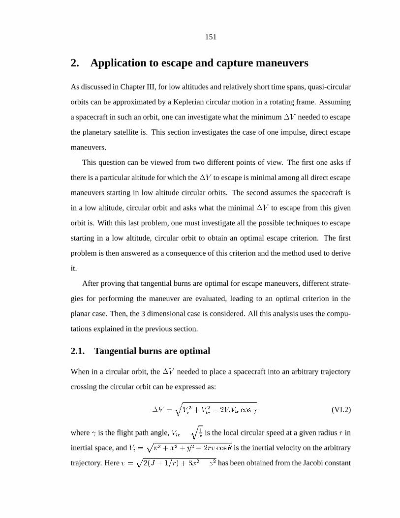
151

2. Application to escape and capture maneuvers

As discussed in Chapter III, for low altitudes and relatively short time spans, quasi-circular

orbits can be approximated by a Keplerian circular motion in a rotating frame. Assuming

a spacecraft in such an orbit, one can investigate what the minimum needed to escape

the planetary satellite is. This section investigates the case of one impulse, direct escape

maneuvers.

This question can be viewed from two different points of view. The first one asks if

there is a particular altitude for which the to escape is minimal among all direct escape

maneuvers starting in low altitude circular orbits. The second assumes the spacecraft is

in a low altitude, circular orbit and asks what the minimal to escape from this given

orbit is. With this last problem, one must investigate all the possible techniques to escape

starting in a low altitude, circular orbit to obtain an optimal escape criterion. The first

problem is then answered as a consequence of this criterion and the method used to derive

it.

After proving that tangential burns are optimal for escape maneuvers, different strate-

gies for performing the maneuver are evaluated, leading to an optimal criterion in the

planar case. Then, the 3 dimensional case is considered. All this analysis uses the compu-

tations explained in the previous section.

2.1. Tangential burns are optimal

When in a circular orbit, the needed to place a spacecraft into an arbitrary trajectory

crossing the circular orbit can be expressed as:

# (VI.2)

where is the flight path angle, is the local circular speed at a given radius in

inertial space, and # # # is the inertial velocity on the arbitrary

trajectory. Here # # has been obtained from the Jacobi constant

152

and represents the inclination in the rotating frame.

Figure VI.8 shows the numerical computation of along the stable manifold as-

sociated with the libration point . As it appears clearly, achieves a minimum at

periapsis and the value of this minimum is, remarkably, equal to one.

1

1.1

1.2

1.3

1.4

1.5

1.6

1.7

1.8

1.9

2

0 0.1 0.2 0.3 0.4 0.5 0.6 0.7

DV

r

-60

-40

-20

0

20

40

60

80

0 0.1 0.2 0.3 0.4 0.5 0.6 0.7

flight path angle (deg)

r

Figure VI.8: as computed along the stable manifold associated with

In the planar case, heuristic argument can be used to show that reaches its minima

at the periapsis passages of the trajectory considered. Indeed, near periapsis, the motion

is very fast and the change in orbital elements are small. Thus, as a first approximation,

one can consider the motion to be represented by a Keplerian motion in a rotating frame.

That is, we let and

, where denotes the

semi-latus rectum and is the true anomaly.

In this approximation, it can be checked that:

where

#

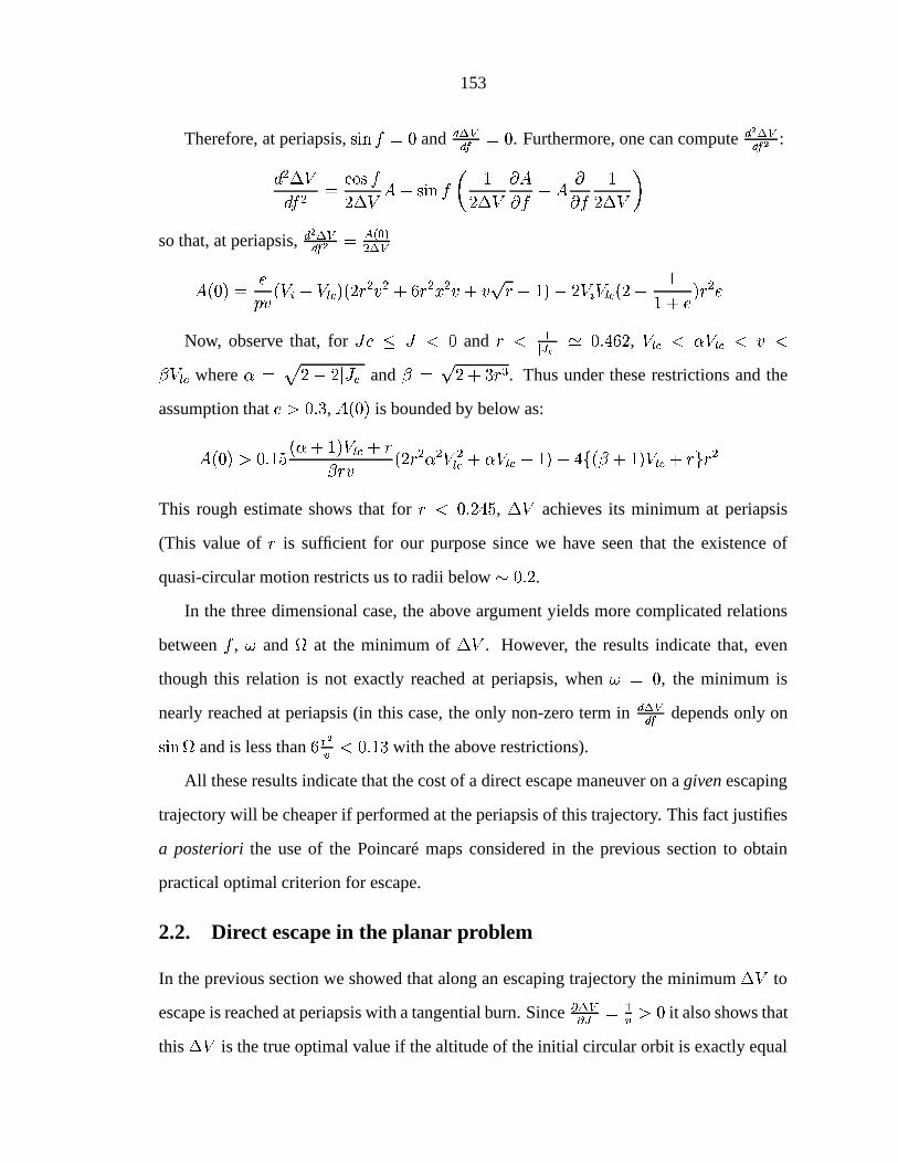
153

Therefore, at periapsis, and . Furthermore, one can compute

:

#

#

so that, at periapsis, "

# #

#

Now, observe that, for and ,

where

and

# . Thus under these restrictions and the

assumption that , is bounded by below as:

# # # # #

This rough estimate shows that for , achieves its minimum at periapsis

(This value of is sufficient for our purpose since we have seen that the existence of

quasi-circular motion restricts us to radii below

.

In the three dimensional case, the above argument yields more complicated relations

between , and

at the minimum of . However, the results indicate that, even

though this relation is not exactly reached at periapsis, when , the minimum is

nearly reached at periapsis (in this case, the only non-zero term in depends only on

and is less than with the above restrictions).

All these results indicate that the cost of a direct escape maneuver on a given escaping

trajectory will be cheaper if performed at the periapsis of this trajectory. This fact justifies

a posteriori the use of the Poincaré maps considered in the previous section to obtain

practical optimal criterion for escape.

2.2. Direct escape in the planar problem

In the previous section we showed that along an escaping trajectory the minimum to

escape is reached at periapsis with a tangential burn. Since

it also shows that

this is the true optimal value if the altitude of the initial circular orbit is exactly equal

154

to the periapsis radius of the stable manifold of . However, for arbitrary this case

is not met in general. Two strategies for escape are then possible. The first one consists

of considering a larger value of so that the Poincaré map reaches the given radius (i.e.,

). Then, a tangential burn is applied at the periapsis of an escaping

trajectory. We indeed saw in the subsection VI.1.3 that the range of altitudes reached by

increases as increases. The second strategy, only applicable for , consists of

performing a non-tangential burn to place the spacecraft on the stable manifold of . For

, only the first strategy is applicable in the case of single impulse, direct escape

maneuvers. Figure VI.9 illustrates the geometry of these two strategies.

Escaping trajectory

Tangential burn

Initial low altitude circular orbit

J>JL2

a

Escaping trajectory(stable manifold of L2)

Non-tangential burn

Initial low altitude circular orbit

J=JL2

b

Figure VI.9: Strategies to escape. (a) First strategy: increase and perform a tan-gential burn. (b) Second strategy: non-tangential burn to place the spacecraft intothe stable manifold associated with or .

Let’s for now assume and compare these strategies. To do so, we compute

the minimum possible using the first strategy, the corresponding to the second

approach being greater than or equal to 1.

Minimum as a function of

For , is not reduced to a single point and on this set, is a function of radius

and longitude of periapsis . We can show that for

,

and that the

minimum is reached on the boundary of the Poincaré map at a point close to (but not

155

equal to) the maximal radius point in the Poincaré map. Denoting this minimal

value at a given , we can numerically compute this value at several values of the Jacobi

constant. The altitude at which is reached increases with so that we can also

compute , which is more convenient from a practical point of view. Figure VI.10

gives the results of such a computation.

We clearly see that decreases as a function of . This result allows us to choose

the first strategy as being optimal. Indeed, for " , " where

" . Now " " where corresponds to the

calculated at any point of an escape trajectory having " as periapsis (by the

optimality of tangential burns). Therefore, " " for any , in

the Poincaré map at a given Jacobi constant . By the fact that decreases as

increases, we see that this inequality is, in fact, satisfied for any " .In particular, " , i.e., the first strategy for escape is more optimal

than the second strategy.

For " , no optimality of " has been proven . In the case of non-

optimality, this result is, thus, only sufficient.

Optimal criterion

For , the strategy to escape is similar to the case . However, in this case,

the minimum to escape does not correspond to the minimum taken over the set

. It is reached at a point near (but not exactly at) . From a practical point of view,

is considered as an optimal solution in this case.

When applying a tangential burn at a given point, the elements of the transfer trajectory

are fixed at periapsis. Therefore, at the time of the maneuver, is equal to the polar angle

(which is approximated by in a circular orbit), which allows us to characterize the

placement of the maneuver in terms of . Using this remark and the results of the previous

i.e., it may happen that (as taken on the boundary of

! ) is slightly less than for slightly greater than . Settling this question depends on evaluating

at a

fixed on the boundary of ! , which is a difficult quantity to compute.

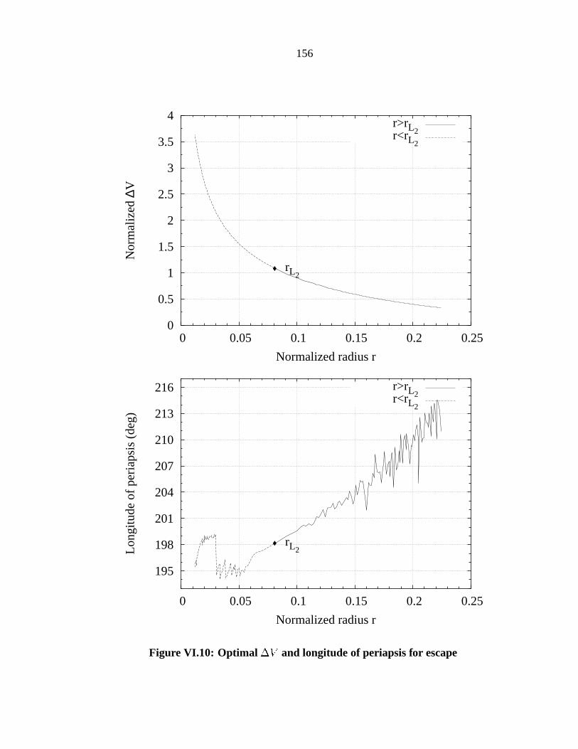
156

0

0.5

1

1.5

2

2.5

3

3.5

4

0 0.05 0.1 0.15 0.2 0.25

Nor

mal

ized

∆V

Normalized radius r

♦ rL2

r>rL2r<rL2

195

198

201

204

207

210

213

216

0 0.05 0.1 0.15 0.2 0.25

Lon

gitu

de o

f pe

riap

sis

(deg

)

Normalized radius r

♦ rL2

♦ rL2

r>rL2r<rL2

Figure VI.10: Optimal and longitude of periapsis for escape

157

sections, we obtain the following escape criterion

:

Starting in a low altitude, circular orbit, at a given radius , fuel optimal

direct escape maneuvers are obtained using an impulsive thrust, tangential

to the path, whose magnitude and placement are determined, respectively,

by and , as given in Figure VI.10 .

We should note that, even though this criterion may be optimal, in practice one would

better use a larger value of to achieve escape since the optimal point lie on the bound-

ary of , which is in . That is, the spacecraft is transfered on trajectory that is caught

in the neck regions for, ideally, an infinite amount of time. This point of optimality is thus

very sensitive to the initial conditions. Applying a larger than this value (at the same

longitude of periapsis), results in increasing so that ! and the point

of the maneuver lies now inside , i.e., the transfer trajectory escapes. This result also

indicates that increasing results in a certain robustness of escape relative to errors in

the initial thrust. In fact, since the optimal point is not isolated, small errors in thrust di-

rection correspond to placing the spacecraft on an escaping trajectory with periapsis near

the optimal value.

Finally, besides quantitatively determining fuel optimal direct escape maneuvers, Fig-

ure VI.10 shows that the answer to the first initial question is negative: there is no optimal

value of such that is minimal among all directly escaping transfers for low circular

orbits. In fact, one can show that there is a minimum for (corresponding to

), but the assumption for a spacecraft to be in a circular orbit at this radius is not

valid anymore and the definition of is less meaningful. Applying our previous results

to the available planetary satellites (whose normalized radius are covered by the range of

Note that, as compared to the results reported in [38], the difference in cannot be seen at theresolution of the graphs given. The only main difference lie in a small difference in the optimal longitude ofthe periapsis.

Because of the limited sampling of the phase space in the numerical procedure, the results for thelongitude of periapsis present some noise for large values of . This appears clearly on this plot, eventhough the computations have been performed with $ $ $ $ points in this case.

158

Jacobi constant considered), we can compute the minimal to escape from these plane-

tary satellites starting in a circular orbit at a low altitude ( ). The savings compared to

a Keplerian escape maneuver (parabolic trajectory) are also computed and summarized in

Table VI.1. Note that savings on the order of in the case of Europa are obtained.

Table VI.1: Minimum to escape the surface of some planetary satellites

Planet Satellite Non- Keplerian Savings when

dimensional scale factor to escape to escape comp. to

( ) ( ) ( ) Kepler. ( )Earth Moon 2.79 235.4 656.8 695.7 38.9

Mars II Deimos 0.44 1.9 0.8 1.9 1.1

Jupiter I Io 0.76 624.7 474.8 748.7 273.9

II Europa 1.12 402.9 451.2 590.9 139.7

III Ganymede 1.44 464.9 669.5 802.8 133.3

IV Callisto 2.04 315.0 642.6 716.0 73.4

X Lysithea 2.75 1.1 3.0 3.3 0.3

Saturn II Enceladus 0.38 64.0 24.3 58.2 33.9

III Thethys 0.52 123.8 64.4 126.3 61.9

IV Dione 0.75 123.1 92.3 146.6 54.3

V Rhea 1.00 139.0 139.0 193.5 54.5

VI Titan 2.02 345.3 697.5 775.6 78.13

VII Hyperion 2.08 15.7 32.7 36.3 3.6

Uranus I Ariel 0.75 137.5 103.1 163.5 60.4

II Umbriel 0.96 111.0 106.6 151.1 44.5

III Titania 1.53 125.2 191.6 225.8 34.2

IV Oberon 1.92 102.7 197.2 212.5 15.3

V Miranda 0.37 62.0 22.9 57.5 34.6

Neptune I Triton 1.42 260.8 370.3 426.3 56.0

Pluto I Charon 1.58 135.8 214.6 252.4 37.8

159

2.3. Direct escape in the spatial problem

As noticed in the first section, the extrema of and over are reached at some point

in the equatorial plane ( ). This is also true for , for which the minimal value is

reached at . The previous optimal criterion is therefore still valid in 3 dimensional

space. However in this case, one can ask what is the minimum to escape starting in a

non-zero inclination initial orbit.

Variations in inclination

As varies, the ranges of inclination reached by the Poincaré maps increase, reaching

rather large values for relatively large values of (see Figure VI.7).

The radius where the maximal inclination is reached decreases with . However, it is

still true that at any fixed , the maximum in inclination increases with . Figure VI.11

gives the envelope curve of a series of Poincaré maps at several values of Jacobi constant,

projected onto the space.

By projecting the data points representing on the plane, it is observed that, to

within the accuracy of the discretization, all these extrema are reached at some point of

the equatorial plane.

Strategy to escape starting in a non-zero inclined orbit

The above remark, and the results discussed on the optimality of tangential burns show

that tangential maneuvers are optimal when compared to non-tangential ones at the points

where the inclination achieves some extrema. This leads us to choose the same approach

to the problem as in the planar case (see subsection “Strategies to escape”).

Starting from a non-zero inclination, low altitude, circular orbit (determined by the

radius and the inclination ), the strategy to escape consists of increasing so that the

maximal inclination reached by the Poincaré map at the given radius equals the initial

inclination . Then, a tangential maneuver is applied at this point of maximal inclination

(at fixed radius ). Since we know that this maximum is reached in the equatorial plane

160

0

5

10

15

20

25

30

35

40

0 0.05 0.1 0.15 0.2 0.25

Incl

inat

ion

i (de

g)

Normlaized radius r

♦rL2

J=-2.163J=-2.16 J=-2.15 J=-2.12 J=-2.05

Figure VI.11: Envelopes of the projections of a few Poincaré maps ( ) onto the space

0

0.5

1

1.5

2

2.5

3

3.5

0.05 0.1 0.15 0.2

Nor

mal

ized

∆V

Normalized radius r

♦rL2

J=-2.05

Figure VI.12: Projection of a Poincaré map onto the space

161

( ), we have the condition ! at the time of the maneuver. The longitude of the

ascending node at such point is restricted to lie in the range , as determined

by Figure VI.6.

Next arises the question of the optimality of such an approach, for which no definite

result is given in this paper. However, a hint at the near optimality of such an approach is

given in Figure VI.12, which presents the projection of a Poincaré map onto the space. We can see on this graph that, at any fixed radius and Jacobi constant , the

variations of over the cross-section of the Poincaré map is very small (less than 0.05).

In fact, as decreases, the thickness of the cross-sections decreases as well, so that for

all the values of considered in this paper, the variations of over a Poincaré map

at a fixed radius are less than 0.05. Moreover, since, as increases, increases at

any fixed point, it can be concluded that, in the case of non-optimality of the previous

approach, the value obtained is very close to the true optimum.

Thus, this may be sufficient from a practical point of view. For example, less than

error on the total costs in the case of Europa are due to the small variations of across at fixed radius .

CHAPTER VII

FUTURE DIRECTIONS

This chapter concludes the dissertation by summarizing the results obtained and discussing

some thoughts on possible research directions.

1. Summary of the results obtained

As we have seen in the previous chapters, the central theme of this dissertation lies in the

idea of periapsis Poincaré maps (which capture the notion of orbital dynamics) and the use

of body perturbations to help achieve orbital control objectives at reduced costs.

1.1. Periapsis Poincaré maps

The investigation of the concept of periapsis lead us to very simple but interesting results

that are a beautiful generalization of the two body problem dynamics. We have seen

indeed that for each value of the Jacobi constant, the position space is partitioned into

exclusively periapsis and apoapsis regions by pairs of surfaces defined as the zero loci of

a six degree polynomial ( ). These pairs of surfaces are delimited by a “mean”

surface ( ) which is a scaled version of the surface of zero velocity. In the Kepler

problem, this mean surface is represented by the set of circular orbits (at a given values

of energy) and the surfaces collapse into this mean surface. This situation is

very similar to the analogy between the zero velocity surfaces in the Hill problem and the

Kepler problem.

We have seen that a direct application of these curves is that the tori of quasi-periodic

162

163

motion predicted by the KAM theory must lie close to these curves, giving us an idea of the

variations of these tori with the Jacobi constant. These results also indicate that retrograde

motion seems more stable than the direct case , a fact also observed in the stability of

periodic orbits [12].

Periapsis Poincaré maps also appear as a natural arena to analyze orbital transfers and,

in particular, are well suited to check the non-impact condition for transfer trajectories.

The use of Picard’s method of successive approximations allows us to derive approxi-

mate expressions for these maps, yielding a first qualitative idea of the short term dynamics

in the Hill problem, notably, the ‘quadrant rule’ of the planar problem that has been ob-

served by several authors has been generalized to the spatial problem.

These estimates also show that body forces can be controlled by the longitude of

the ascending node and the argument of periapsis of a transfer trajectory, thus opening the

way for the use of these forces in orbital control purposes.

Thus, it appears that the concept of periapsis is very useful in many orbit transfers and

the features of the periapsis Poincaré maps should be investigated in connection with other

problems in astrodynamics.

1.2. Third body driven transfers

A new way of performing plane changes in an orbital environment perturbed by a body has been investigated both for its own interest, and as an example of a body

driven maneuver.

These body driven plane changes are performed using two impulsive maneuvers

and a timing of the first burn, resulting in transfers analogous to the bi-elliptic plane

changes, but with the apoapsis maneuver suppressed. It has been shown that these trans-

fers can improve the classical one impulse results by lowering the required for plane

change values larger than ! . Savings on the order of have been obtained for large

plane changes ( ! ) and the possibility of a reversal of the direction of motion has been

164

shown to exist using such an approach.

Besides these results, the analysis performed shows that interesting information can be

obtained with the help of the Jacobi constant, yielding in our case an analytical estimate

of the limit of optimality between body driven plane changes and one impulse maneu-

vers and a significant simplification of the numerical algorithm used to solve the design

problem. This method may be applicable to other problems of astrodynamics.

1.3. Escape and Capture maneuvers

Escaping and capture trajectories in the Hill three body problem have been investigated

using a Poincaré map. This map allows us to characterize the set of periapses before escape

(or, after capture) by some bounds on radius, longitude of periapsis and inclination.

These results show, in particular, that very low energy capture trajectories cannot be

performed for all planetary satellites since the capture trajectories would impact the surface

of the primary before reaching periapsis.

These results have also been applied to the problem of determining the minimum needed to escape from a planetary satellite, starting in a low altitude, circular orbit. An

optimal criterion has been given in the planar case and a practical approach has been given

in the three dimensional case. It is shown that the resulting cost for escape decreases as

the initial altitude increases. The cost to escape in the vicinity of a planetary satellite is on

the order of the scale factor, , and represents significant savings as compared

to a parabolic escape.

2. Possible future research directions

In this section we outline some possible directions of research that emerge from the pre-

ceding work. Two main lines of investigation can be envisioned, one related to the peri-

apsis Poincaré maps (tools of investigation) and the other would be more focused on the

applications to orbital transfers.

165

2.1. Periapsis Poincaré maps

The idea of periapsis limiting curves can be applied to the restricted three body problem

or other astrodynamical problems such as the asteroid or binary asteroid problems. As we

have seen, while involving rather simple calculations, these curves can yield information

on the qualitative behavior of quasi-circular motion and may be used to corroborate results

obtained by other means.

A second path of research would be to develop computer algebra techniques to deal

with higher order estimates of the periapsis Poincaré maps. These techniques would allow

us to apply the method of periapsis Poincaré maps to other astrodynamical systems and

yield more accurate information on the dynamics than first order estimates. This would

lead to a software tool that could be used to analyze multiple loop transfers or optimization

problem with path constraints, such as a non-impact condition.

2.2. Further transfers

The limitations encountered on the range of body driven plane changes due to the sole

use of the natural dynamics can be removed by performing plane changes at the first and

last burn. With the addition of an apoapsis maneuver, these transfers would generalize the

classic full three impulse plane change to the case of body perturbed environments,

improving the savings obtained here. This approach would unconditionally improve on

the classical results and may appear as the optimal method over all the possible impulsive

transfers in such environments.

Other orbital objectives could also be analyzed in the body perturbed environments,

the most direct extension of these results presented being the case of simultaneous radius

change and plane change maneuvers. Instead of computing the zero lines of , one has

to compute the lines where represents the amount of desired radius change.

Though larger savings may be possible in such cases, the order of magnitude of the savings

obtained for the case should be attainable since these zero lines correspond to

166

a change of sign of the function , so that performing the first maneuver a little

ahead or after the values considered in this dissertation should yield a positive or negative

net change in periapsis radius while keeping the values of plane change realized with

the zero periapsis change. This may be of interest for safety issues where a decrease in

periapsis radius is generally not desirable.

Third body driven transfer ideas could also be used in conjunction with other transfer

techniques used in interplanetary mission. For example, as the body driven maneuvers

involve raising the apoapsis radius to a significant distance from the central body, third

body effects together with fly-bys of other celestial bodies in the vicinity of the primary,

e.g., the Moon in the Earth environment, could be used to perform cheaper transfers. An-

other example would be to use the control of and

in conjunction with aerocapture

techniques to decrease the energy of a spacecraft upon arrival at Mars faster than with the

sole use of the aerocapture technique, thus shortening the travel time from Earth to Mars.

Finally, escape and capture maneuvers should be investigated further. Notably, results

in the spatial problem should be obtained and multiple loop transfers (i.e., escape after

revolution around the primary) should be investigated. These transfers involve interesting

dynamics that mix transit through both libration points and . Moreover these trans-

fers could be connected with the previous ideas on third body driven transfers to obtain

path constrained transits. That is, one could envision design of capture trajectories that

reach a desired inclination after revolutions around the primary, only with the use of

natural dynamics or with a minimum amount of impulsive control, much in the same spirit

as some of the results reported in [11].

APPENDIX A

SYMPLECTIC TRANSFORMS, JACOBICOORDINATES AND KEPLER PROBLEM

This appendix reviews the basics facts about symplectic transformations, the Jacobi coor-

dinates and the Kepler problem.

1. Symplectic transformations with multipliers

Symplectic transformations were defined classically as transformations that leave the form

of Hamilton’s equations invariant. As such, there are no restrictions on the form of the

Hamiltonian, provided that the transformed variables satisfy Hamilton’s equations with

the new Hamiltonian. With this definition, it has been shown by Wintner [43]that a trans-

formation is symplectic if and only if:

(A.1)

where

is the symplectic matrix and is non-zero and is called the mul-

tiplier of the transformation ( and

are the identity and zero elements of the ,

respectively). In this case the original Hamiltonian is transformed into the new

Hamiltonian .These transformations are also called symplectic transformations with multiplier , to

reserve the appellation symplectic transformation to the case where .

These transformations with multiplier allow us to scale the variables ’canonically’ in

Hamiltonian systems. For example, if and , then the

167

168

transformation:

is symplectic with multiplier .2. Application to the Kepler problem

When in a frame with origin at the center of mass of the frame, the two body problem

reduces to the Kepler problem. That is, the Kepler problem represents the relative motion

of two point mass particles interacting gravitationally. Expressed in a rotating frame, this

problem is given by the Hamiltonian:

where is sometimes called the reduced mass of the system. In fact, Kepler’s

problem depends only on one parameter, the total mass of the system. The following

symplectic transformation with multiplier makes this fact apparent:

; ;

where # is the gravitational parameter of the system.

In this form, we see also that Kepler’s problem can be interpreted as the motion of a

unit mass in a central gravitational field (fixed center) of strength . This interpretation

leads to the restricted two body problem when one of the masses is much smaller than

the other one. For example, in the case of , # . Even though

these two problems represent two different situations, they are represented by the same

set of equations and the restricted two body problem is generally referred to as the Kepler

problem, as well.

Now observe that the equations of motion are given by: #

169

Thus and

when and

are constant (say, " and " , respectively) and

we obtain the following relations: " " " "These solutions represent relative equilibria of the Kepler problem and correspond to

circular orbits in the inertial space.

For these solutions, the angular velocity is related to the orbit raidus. Indeed, from the

above relations we obtain:

" "and, denoting the angular speed of the frame:

In order to investigate the motion close to a relative equilibrium, one can look at small

perturbations from these solutions. That is, we let:

" " This transformation is symplectic, and, applying Taylor’s expansion theorem to the

Hamiltonian, one obtains:

" " # " "

# " "

#

Since " " is a relative equilibrium, " "

. Also, the constant term

is generally dropped since it does not change the equations of motion. The Hessian

170

is given by:

" "

and the higher order terms only involve the terms ( ), and these

terms scale with as . That is, if we let " , scales as since the term is fixed. Thus, we find that

" " #

3. Symplectic completion

A simple but useful operation related to symplectic transformations is the process of

symplectic completion, that is the extension of a point transformation on configuration

space into a symplectic transformation in phase space. This process was first analyzed by

Matthieu and are also referred to as Matthieu transforms.

Let be a point transformation on configuration space (any smooth mani-

fold). Then one can complete this transformation into a symplectic transformation with

multiplier by transforming the corresponding momenta

according to such

that:

(A.2)

Indeed, let

denote the transformation from the to the variables. That

is, . Then:

so that

171

and, upon imposing the relation (1), one arrives at (2).

In the particular case of a linear transformation where

is non-

singular, one obtain a symplectic transformation with multiplier by transforming the

momenta according to . Similarly, the symplectic completion of

is .

4. Application to the Jacobi coordinates

In Chapter II, we defined the Jacobi coordinates from the

variables the the variables

by choosing " to represents the position of the center of mass of the three particles, to represents the relative position of the second particle with respect to the first particle

and to be the position of the third particle with respect to the center of mass of the first

two particles, as is illustrated in Figure II.1. That is, we made the point transformation , where:

where # # .

Then we immediately obtain the conjugate momenta so that transforma-

tion is is symplectic. can easily be computed as:

and we readily obtain the formulas given Chapter II (equations (II.6)-(II.6)).

APPENDIX B

SCALING TO PLANETARY SATELLITES

The following table (1) give the length and time scales of all the planetary satellites in the

solar system whose mass, orbital period and radius are known [35].

The length and time scales, and are the unit length and time scales

used to normalize the Hill equations in Chapter II. The type has been defined in Chapter

VI. A planetary satellite is of type 1 if the first periapsis of the stable manifold of the

libration points and are below the physical surface of the satellite. It is of type 2

otherwise.

172

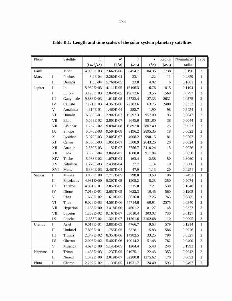
173

Table B.1: Length and time scales of the solar system planetary satellites

Planet Satellite # Radius Normalized Type

( ' ! ) ( $ ) ( ) ( ) ( ) radius

Earth Moon 4.903E+03 2.662E-06 88454.7 104.36 1738 0.0196 2

Mars I Phobos 6.4E-04 2.280E-04 23.1 1.22 11 0.4859 1

II Deimos 1.3E-04 5.760E-05 33.8 4.82 6 0.1881 1

Jupiter I Io 5.930E+03 4.111E-05 15196.3 6.76 1815 0.1194 1

II Europa 3.193E+03 2.048E-05 19672.6 13.56 1569 0.0797 2

III Ganymede 9.883E+03 1.016E-05 45733.4 27.33 2631 0.0575 2

IV Callisto 7.171E+03 4.357E-06 72283.6 63.75 2400 0.0332 2

V Amalthea 4.814E-01 1.460E-04 282.7 1.90 98 0.3454 1

VI Himalia 6.335E-01 2.902E-07 19592.3 957.09 93 0.0047 2

VII Elara 5.068E-02 2.801E-07 8645.0 991.80 38 0.0044 2

VIII Pasiphae 1.267E-02 9.894E-08 10897.8 2807.49 25 0.0023 2

IX Sinope 5.070E-03 9.594E-08 8196.2 2895.35 18 0.0022 2

X Lysithea 5.070E-03 2.805E-07 4008.2 990.15 81 0.0202 2

XI Carme 6.330E-03 1.051E-07 8308.9 2643.25 20 0.0024 2

XII Ananke 2.530E-03 1.152E-07 5756.7 2410.24 15 0.0026 2

XIII Leda 3.800E-04 3.046E-07 1600.0 911.84 8 0.0050 2

XIV Thebe 5.068E-02 1.078E-04 163.4 2.58 50 0.3060 1

XV Adrastea 1.270E-03 2.438E-04 27.7 1.14 10 0.3606 1

XVI Metis 6.330E-03 2.467E-04 47.0 1.13 20 0.4251 1

Saturn I Mimas 3.035E+00 7.717E-05 798.8 3.60 196 0.2453 1

II Enceladus 4.931E+00 5.307E-05 1205.2 5.23 250 0.2074 1

III Thethys 4.931E+01 3.852E-05 3215.0 7.21 530 0.1648 1

IV Dione 7.018E+01 2.657E-05 4632.3 10.45 560 0.1208 1

V Rhea 1.669E+02 1.610E-05 8636.0 17.26 765 0.0885 1

VI Titan 9.028E+03 4.561E-06 75714.8 60.91 2575 0.0340 2

VII Hyperion 1.138E+00 3.418E-06 4601.2 81.27 148 0.0322 2

VIII Lapetus 1.252E+02 9.167E-07 53010.4 303.02 730 0.0137 2

IX Phoebe 2.655E-02 1.321E-07 11501.6 2102.68 110 0.0095 2

Uranus I Ariel 9.017E+01 2.885E-05 4766.7 9.63 579 0.1214 1

II Umbriel 7.803E+01 1.755E-05 6328.1 15.83 586 0.0926 1

III Titania 2.347E+02 8.353E-06 14982.5 33.25 790 0.0527 2

IV Oberon 2.006E+02 5.402E-06 19014.2 51.43 762 0.0400 2

V Miranda 4.624E+00 5.145E-05 1204.4 5.40 240 0.1992 1

Neptune I Triton 1.433E+03 1.237E-05 21075.1 22.45 1353 0.0642 2

II Nereid 1.372E+00 2.019E-07 32280.8 1375.62 170 0.0052 2

Pluto I Charon 2.202E+02 1.139E-05 11931.7 24.40 593 0.0497 2

APPENDIX C

REDUCED CUBIC EQUATIONS

This appendix reviews the basic results about reduced cubic equations and applies these

results to the zero velocity surfaces defined in Chapter III. The book by Conkwright [8]

has been used as a reference for the cubic equation.

1. Basic results

A reduced cubic equation is an equation of the form:

# # (C.1)

where the variable is a priori a complex number and we restrict ourselves to the case of

and real.

In this case, Descartes’ rule in conjunction with the sign of the discriminant, allows us

to determine the number of positive and negative roots of the equation. More precisely,

Descartes’ rule consists of counting the numbers of change of sign between the coeffi-

cients. Then, it follows that the number of positive roots differs from this number by an

even integer. For example, if is negative and is positive, there is two change of signs

and thus the equation (3) has zero or two positive roots. If and are both positive,

this rule ensures that there is exactly one positive root. By applying Descartes’ rule to

the equation obtained by replacing by , one can obtain some informations about the

number of negative roots.

174

175

The discriminant rule consists of computing the discriminant of the reduced cubic

equation:

# (C.2)

and then applying the following result:

if

, then equation (3) admits exactly one real root.

if , then equation (3) admits a double root.

if , then equation (3) admits three distinct real roots.

When Descartes’ rule informed us that the equation (3) has or positive roots, the

discriminant can tell us which number to choose. If

then there is zero positive root,

whereas if then the equations admits exactly two positive roots. This last statement

is not a direct consequence of the discriminant rule but follows from the specific form of

the reduced cubic equation. Indeed, when , the three roots of (3) are given by:

# (C.3)

where

, .

From this form of the solution, it is clear that when the reduced cubic has three distinct

real roots, at least one of them is negative. Thus the result follows.

When , so that depending on the sign of . The roots

are given in this case by:

; ; where represents the sign of .

When

, the only real root is given by Cardan’s formula:

# #

#

# (C.4)

176

When and are function of a parameter (as in the case of the defining equation of

the zero velocity surfaces), the roots of 3) are also continuous functions of the parameter.

For example, if , and (3) has exactly two positive roots and if a change in the

parameter results in setting , then the two positive roots collapse at

. If further

change in the parameter results in

, then we know that the only real root will be

negative. Moreover, in this case, the two positive roots (when ) are separated by

the collapse value so that one root will increase towards while the other root will

decrease towards this value. This situation occurs when goes from to ,

starting first on the x-axis. For , and the two positive roots correspond to

the two components of and the value of separates these components. When

, the roots collapse at . For , there are no longer any

positive roots and the zero velocity surface is now open.

2. Application to the zero velocity surfaces

Recall that the zero velocity surface, , is defined as the zero loci of the reduced cubic

equation:

# #

where , and and is non-zero (In

the case , the above cubic equation reduces to for and has no real

positive solutions for ).

From (4), we see that #

, and the sign of

is determined by

the sign of # .

Now, applying the above results (Descarte’s and discriminent rules), we obtain the

charaterization of the roots presented in Table 2.

In order to check the critical points of the roots, , of (3) with and

, we first note

that depends on and

only through , so that these critical points are obtained when

(when defined).

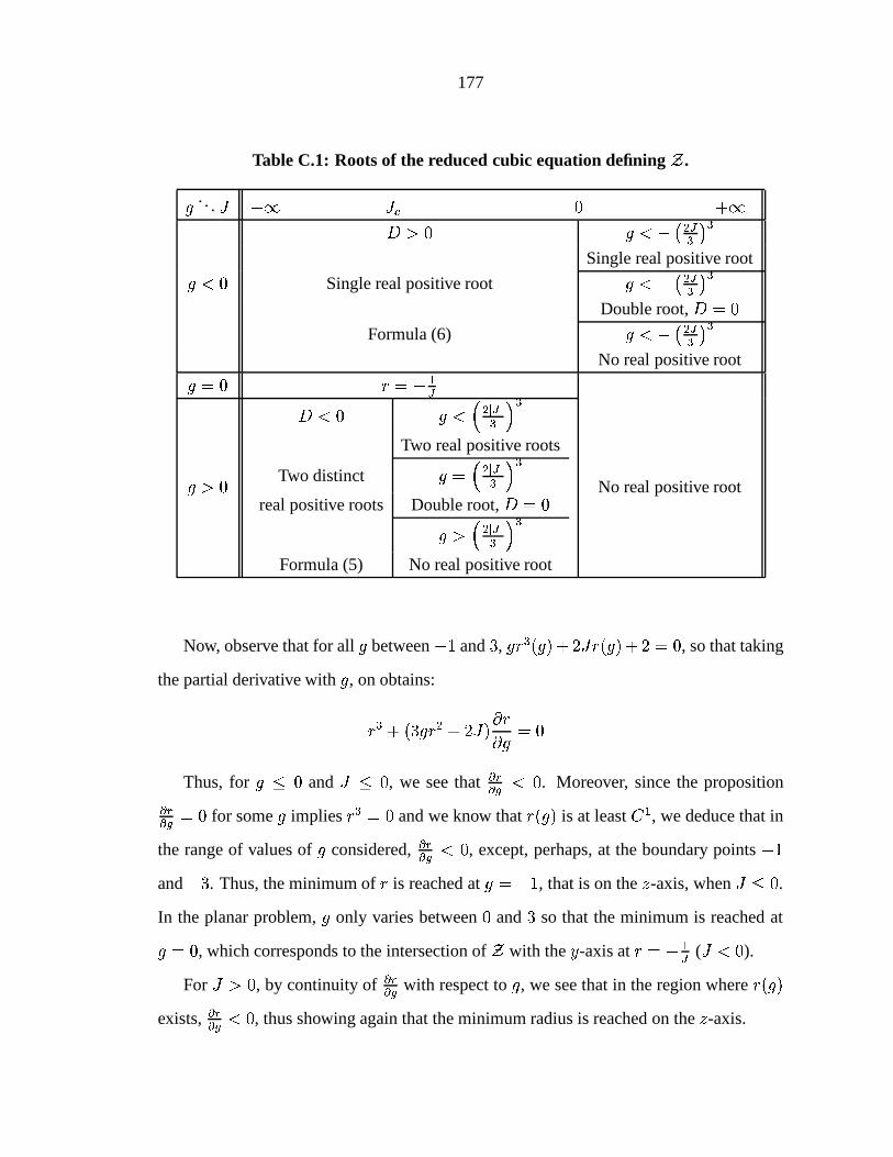
177

Table C.1: Roots of the reduced cubic equation defining .

. . . #

Single real positive root

Single real positive root

Double root,

Formula (6)

No real positive root

Two real positive roots

Two distinct real positive roots Double root,

Formula (5) No real positive root

No real positive root

Now, observe that for all between and , # ! # , so that taking

the partial derivative with , on obtains:

# #

Thus, for and , we see that

. Moreover, since the proposition

for some implies and we know that is at least , we deduce that in

the range of values of considered,

, except, perhaps, at the boundary points

and . Thus, the minimum of is reached at , that is on the -axis, when .

In the planar problem, only varies between and so that the minimum is reached at

, which corresponds to the intersection of with the -axis at ( ).

For , by continuity of with respect to , we see that in the region where exists,

, thus showing again that the minimum radius is reached on the -axis.

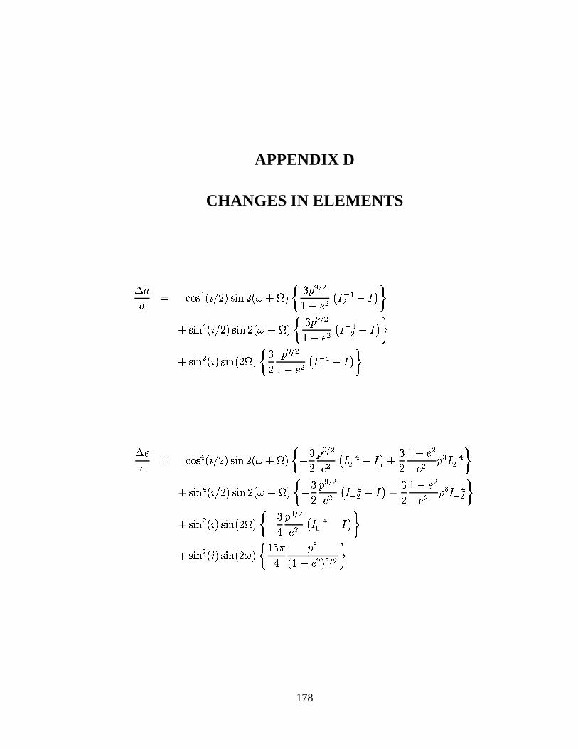
APPENDIX D

CHANGES IN ELEMENTS

#

#

#

"

#

#

#

#

#

" ! #

178

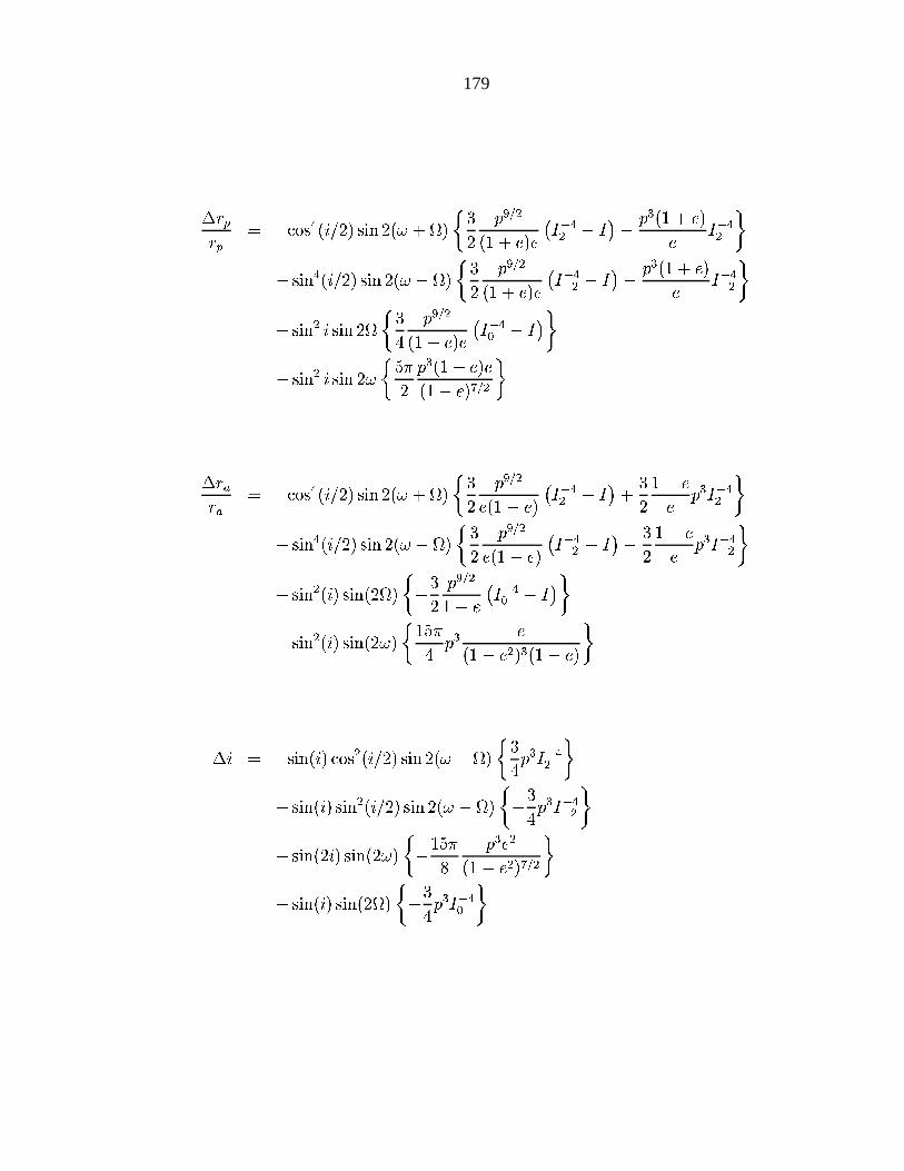
179

#

# #

# #

#

# "

#

#

! #

#

"

#

#

#

#

#

"

APPENDIX E

NUMERICAL INTEGRATION

Throughout this work, a Runge-Kutta-Felhberg type integrator of order has been used

for the numerical integrations, with accuracy of "

per step. That is, an embedded

order Runge-Kutta method is used in an order scheme to estimate the truncation error

made at each step and correct the time step in order to meet the desired accuracy.

The results presented in Table IV.2 have been obtained from the data of an integrated

trajectory with DPTRAJ, communicated by M.D. Guman. The following paragraph, also

due to M.D. Guman, briefly presents this integration.

DPTRAJ is a high accuracy trajectory computation program developed at the Jet Propul-

sion Laboratory for use in the navigation and design of space missions [10]. It is an accu-

rate and general spacecraft trajectory program due to its ability to model all relevant force

perturbations found in the solar system to high levels of precision. In order to simulate the

“real” orbit dynamics of the Europa orbiter we use this program with a complete suite of

force models. In the runs made for this analysis these force models included gravitational

perturbations from the Sun and planets, the Galilean satellites (Io, Ganymede, Callisto,

and Europa of course), ! and for Jupiter and the Europa gravity field up to de-

gree and order. Also incorporated are the non-gravitational perturbations of the Europa

atmosphere and solar radiation pressure.

180

Bibliography

[1] D.F. Appleyard. Invariant Sets near the Collinear Lagrangian Points of the Nonlin-

ear Restricted Three-Body Problem. PhD thesis, University of Wisconsin, 1970.

[2] V.I. Arnol’d. Dynamical systems III. Encyclopedia of Mathematical Sciences.

Springer-Verlag, 1988.

[3] V.I. Arnol’d. Small denominators and problems of stability of motion in classical

and celestial mechanics. Russian Mathematical Surveys (published by the London

Mathematical Society), 18(6), Nov-Dec. 1963.

[4] E.A. Belbruno. Sun-perturbed Earth-to-Moon Transfers with Ballistic Capture. Jour-

nal of Guidance, Control and Dynamics, 16(4), July-August 1993.

[5] J.V. Breakwell and L.M. Perko. Matched asymptotic expansions, patched conics

and the computation of interplanetary trajectories. In Proceedings of the AIAA/ION

Astrodynamics Specialists Conference, pages 291–300, 1965.

[6] B. Chavineau. Dynamique à long terme des astéroides binaires. Bilan des observa-

tions et approche théoriques. Ph.D. thesis. Université de Nice, 1990.

[7] V.A. Chobotov, editor. Orbital Mechanics. AIAA Education Series. American Insti-

tute of Aeronautics and Astronautics, edition edition, 2002.

[8] N.B. Conkwright. Introduction to the Theory of Equations. Blaisdell Publishing

Company, New York, Toront, London, 1965.

181

182

[9] C.C. Conley. Low energy transit orbits in the restricted three-body problem. SIAM

Journal of Applied Mathematics, 16(4):732–746, July 1968.

[10] J.E. Ekelund. DPTRAJ-ODP User’s Reference Manual, volume 1. Jet Propulsion

Laboratory internal memo JPL 642-3405-DPTRAJ-ODP, 1996.

[11] G. Gomez, W.S. Koon, M.W. Lo, J.E. Marsden, J. Masdemont, and S.D. Ross. In-

variant manifolds, the spatial three-body problem and space mission design. In As-

trodynamics Specialist Meeting, pages AAS 01–31, Quebec City, Canada, August

2001.

[12] M. Hénon. Numerical exploration of the restricted problem.v. hill’s case: Periodic

orbits and their stability. Astronomy and Astrophysics, 1:223–238, 1969.

[13] M. Hénon. Generating families in the restricted three-body problem. Lectures Notes

in Physics. New series m. Springer-Verlag, 1997.

[14] M. Hénon. New families of periodic orbits in hill’s problem of three bodies. Celestial

Mechanics and Dynamical Astronomy, 85(3):223–246, March 2003.

[15] M. Hénon and J.M. Petit. Series Expansions for Encounter-type Solutions of Hill’s

Problem. Celestial Mechanics and Dynamical Astronomy, 38:67–100, 1986.

[16] M. Hénon and J.M. Petit. Satellite encounters. Icarus, 66(3):536–555, June 1986.

[17] J. Henrard and J.F. Navarro. Spiral structures and chaotic scattering in coorbital

satellites. Celestial Mechanics and Dynamical Astronomy, 79:297–314, 2001.

[18] G.W. Hill. Researches in the Lunar Theory. American Journal of Mathematics,

1:5–26, 1878.

[19] Kaula. Application of Satellite to geodesy. Dover Science Books, New York, 1960.

183

[20] W.S. Koon, M.W. Lo, J.E. Marsden, and S.D. Ross. Low energy transfer to the moon.

Celestial Mechanics and Dynamical Astronomy, 81:63–73, 2001.

[21] W.S. Koon, M.W. Lo, J.E. Marsden, and S.D. Ross. Heteroclinc connections between

periodic orbits and resonance transitions in celestial mechanics. Chaos, 10(2):427–

469, June 2000.

[22] J. Llibre, R. Martínez, and C. Simó. Transversality of the invariant manifolds asso-

ciated to the lyapunov family of periodic orbits near in the restricted three-body

problem. Journal of Differential Equations, 58:104–156, 1985.

[23] M.W. Lo, B.G. Williams, W.E. Bollman, D.S. Han, Y.S. Hahn, J.L. Bell, E.A. Hirst,

R.A. Corwin, P.E. Hong, K.C. Howell, B. Barden, and R. Wilson. Genesis mission

design. Journal of the Astonautical Sciences, 49(1):169–184, January-March 2001.

[24] K.R. Meyer. Periodic solutions of the n-body problem. Journal of Differential Equa-

tions, 39:2–38, 1981.

[25] K.R. Meyer. Scaling hamiltonian systems. SIAM Journal of Mathematical Analysis,

15(5), September 1984.

[26] K.R. Meyer and G.R. Hall. Introduction to Hamiltonian Dynamical Systems and the

N-body Problem, volume 90 of Applied Mathematical Sciences. Springer-Verlag,

1991.

[27] K.R. Meyer and D.S. Schmidt. Hill’s lunar equations and the three-body problem.

Journal of Differential Equations, 44:263–272, 1982.

[28] O. Montenbruck and E. Gill. Satellite Orbits: models, methods, and applications.

Springer, 2000.

[29] J. Moser. On the generalization of a theorem of a.lyapunov. Communications on

Pure and Applied Mathematics, XI:257–271, 1958.

184

[30] D.J. Scheeres. The restricted Hill four-body problem with applications to the Earth-

Moon-Sun system. Celestial Mechanics and Dynamical Astonomy, 70:75–98, 1998.

[31] D.J. Scheeres. Changes in rotational angular momentum due to gravitational inter-

actions between two finit bodies. Celestial Mechanics and Dynamical Astronomy,

81(1-2):39–44, 2001.

[32] D.J. Scheeres, M.D. Guman, and B.F. Villac. Stability analysis of planetary satel-

lite orbiters: Application to the europa orbiter. Journal of Guidance, Control and

Dynamics, 24(4), July-August 2001.

[33] D.J. Scheeres and F. Marzari. Spacecraft dynamics in the vicinity of a comet. Journal

of Astronautical sciences, 50(1):35–52, January-March 2002.

[34] Scottish Universities Summer School in Physics, editor. The restless Universe: ap-

plications of gravitational n-body dynamics to planetary, stellar and galactic sys-

tems. Copublished by Scottish Universities Summer School in Physics & Institute of

Physics Pub., 2001.

[35] K.P. Seidelmann. Explanatory supplement of the Astronomical almanac. Mill Valley

Calif.: University Science Books, 1992.

[36] C. Simó and T.J. Stuchi. Central stable/unstable manifolds and the destruction of

kam tori in the planar hill problem. Physica D, 140:1–32, 2000.

[37] V. Szebehely. Theory of Orbits. Academic Press, New York, 1967.

[38] B.F. Villac and D.J. Scheeres. Escaping trajectories in the hill three body problem

and applications. Journal of Guidance, Control and Dynamics, 26(2):224–232, 2002.

[39] B.F. Villac and D.J. Scheeres. Optimality of tidally driven plane changes. In Pro-

ceedings of the New trends in Astrodynamics conference, 2003.

185

[40] B.F. Villac and D.J. Scheeres. A new class of optimal plane change maneuvers.

Journal of Guidance, Control and Dynamics, in press.

[41] B.F. Villac, D.J. Scheeres, L.A. D’Amario, and M.D. Guman. The effect of tidal

forces in orbit transfers. In Proceedings of the AAS/AIAA Spaceflight Mechanics

Meeting at Santa Barbara, CA, pages 2049–2070, 2001.

[42] S. Wiggins. Introduction to Applied Nonlinear Dynamical Systems and chaos.

Springer-Verlag, 1990.

[43] A. Wintner. Analytical Foundations of Celestial Mechanics. Princeton University

Press, 1941.

Documents

DYNAMICS IN THE HILL PROBLEM WITH …...DYNAMICS IN THE HILL PROBLEM WITH APPLICATIONS TO SPACECRAFT MANEUVERS by Benjamin F. Villac A dissertation submitted in partial fulﬁllment