Dynamics and motion control Lecture 5 Model following ... · KTH MMK Mechatronics Lab 5.3.7. General remarks • The two concepts of servo control are often combined • Some process

Mechatronics LabKTH MMK

Date: 2009-08-27File: Q:\md.kth.se\md\mmk\gru\mda\mf2007\arbete\Lectures\FinalVersions\For2009\L5.fm

Slide: 1(35)

Dynamics and motion control

Lecture 5

Model following control-servo design

Jan Wikander,Bengt Eriksson

KTH, Machine DesignMechatronics Lab

e-mail: [email protected]



Slide: 2(35)

5.1. Lecture outline

• 1. Introduction

• 2. Transfer function based model following

• 3. Time domain based model following

• 4. An example

• 5. Matlab example for the dc motor



Slide: 3(35)

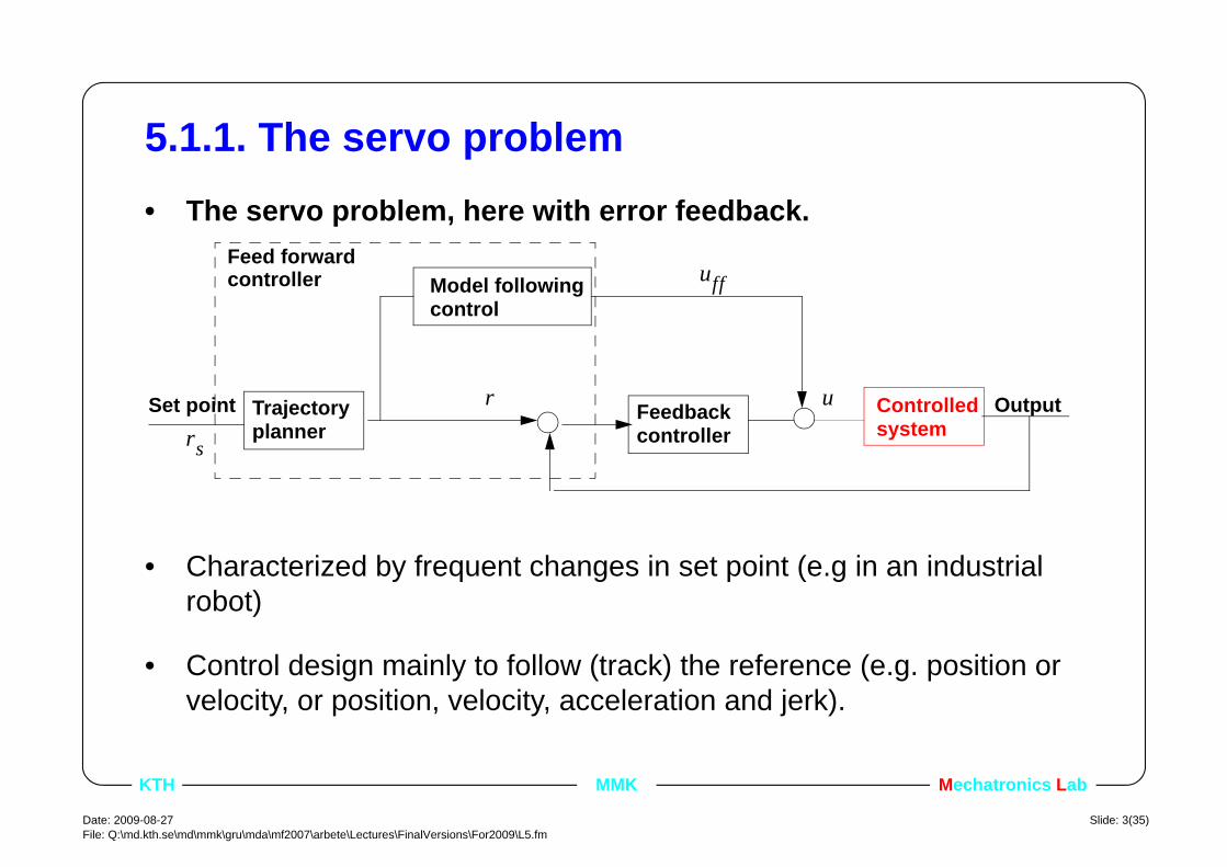
5.1.1. The servo problem• The servo problem, here with error feedback.

• Characterized by frequent changes in set point (e.g in an industrial robot)

• Control design mainly to follow (track) the reference (e.g. position or velocity, or position, velocity, acceleration and jerk).

Controlledsystem

Model followingcontrol

Trajectoryplanner

OutputSet pointrs

ur

uff

Feedbackcontroller

Feed forwardcontroller


Slide: 4(35)


5.1.2. Feedback control properties• The main principle in control engineering

• Typically model based (but not required to be)

• Produces control signals after an error has occurred

• Disturbance rejection is achieved

• Effect of process parameter variations is reduced

• Leads to a closed loop

• Sensor noise may be amplified and deteriorate performance

• May lead to instability if designed incorrectly



Slide: 5(35)

5.1.3. Feed forward control properties

• Model based (but fairly simple models typically helps a lot)

• Produces control signals before error has occurred

• Uses measured or modelled disturbance and compensates for it

• Uses carefully designed reference signals to make the process follow the references “exactly” and without saturating the control signal.

ProcessFeed forwardcontrol

Reference signal

DisturbanceDisturbance (measured or modelled)

Output


Slide: 6(35)


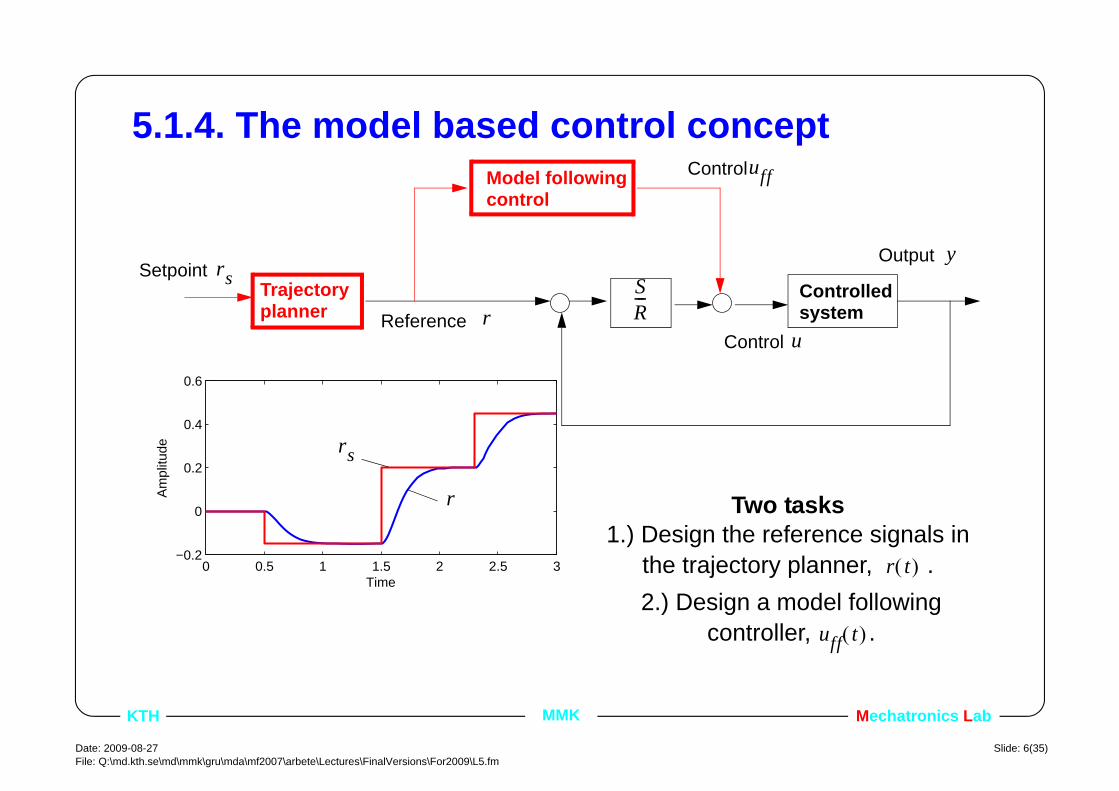
5.1.4. The model based control concept

0 0.5 1 1.5 2 2.5 3−0.2

0

0.2

0.4

0.6

Time

Am

plitu

de rs

r

Controlledsystem


Trajectoryplanner

Output

SR---

Reference

Setpoint

r

yrs

Control u

Controluff

Two tasks 1.) Design the reference signals in

the trajectory planner, . 2.) Design a model following

controller, .

r t( )

uff t( )



Slide: 7(35)

5.1.5. The ultimate goal, Exact model following

• Design the trajectory planner and the model following controller such that the feed forward input signal uff(t) drives the output to the desired setpoint

• Note that the model following control part can be a nonlinear system

• Two main concepts, Transfer function and Time domain.

Controlledsystem


Trajectoryplanner

OutputReference

uff

Set point


Slide: 8(35)


5.2. Lecture outline• 1. Introduction



• 4. An example




Slide: 9(35)

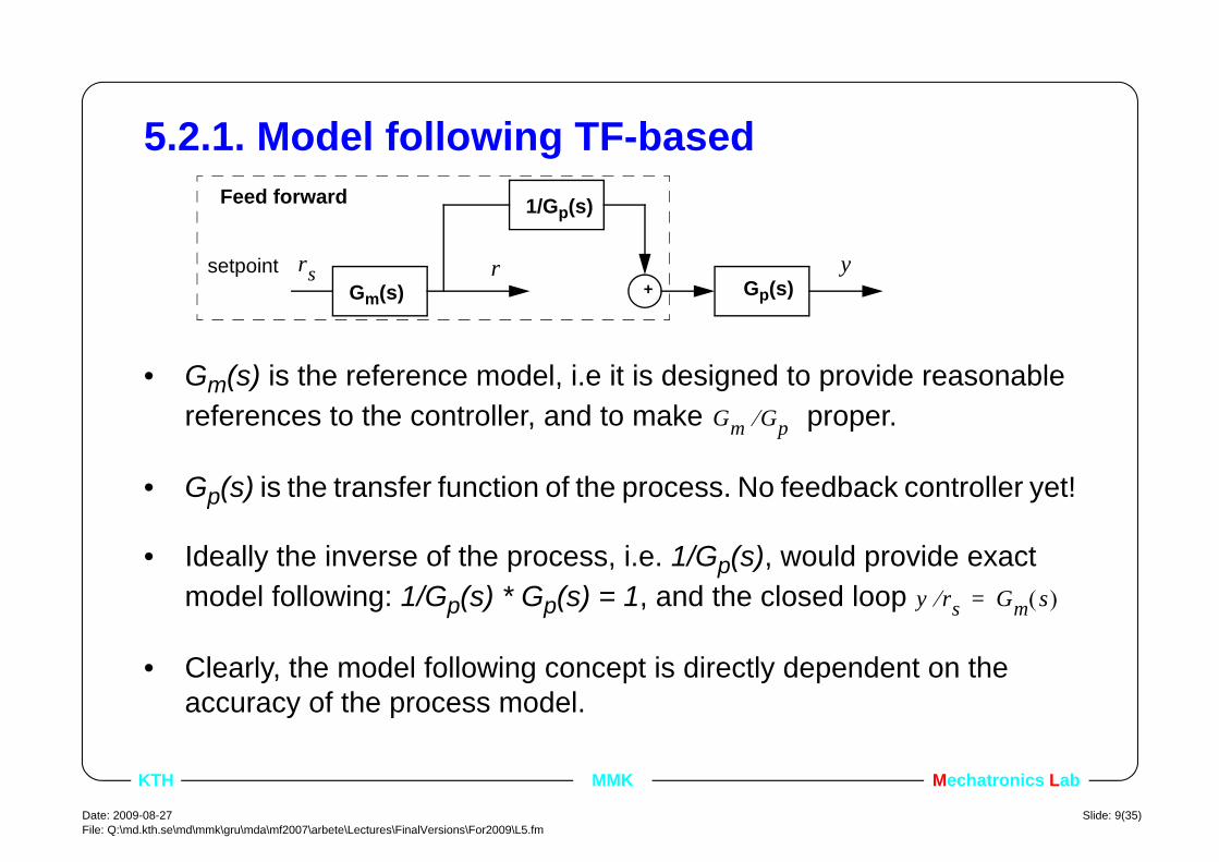
5.2.1. Model following TF-based

• Gm(s) is the reference model, i.e it is designed to provide reasonable references to the controller, and to make proper.

• Gp(s) is the transfer function of the process. No feedback controller yet!

• Ideally the inverse of the process, i.e. 1/Gp(s), would provide exact model following: 1/Gp(s) * Gp(s) = 1, and the closed loop

• Clearly, the model following concept is directly dependent on the accuracy of the process model.

Gp(s)

1/Gp(s)

Gm(s) +setpoint rs r y

Feed forward

Gm Gp⁄

y rs⁄ Gm s( )=


Slide: 10(35)


5.2.2. The reference model Gm(s)

• The task of the reference model is to generate smooth references that the process is able to follow.

• To implement complete model following, i.e a full process inverse, we must require that the pole excess dm of the reference model is larger than or equal to the pole excess d of the process, i.e if

is the pole excess of the process dp

and finally the requirement

Gp s( ) B s( )A s( )-----------=

dp deg A( ) deg B( )–=

dm dp≥ Gm s( )Bm s( )

Am s( )---------------= dm deg Am( ) deg Bm( )–=



Slide: 11(35)

5.2.3. Model following TF-based cont.• Since exact model following involves taking the inverse of the process

model, the inverse must be possible to implement. I.e. the inverse must constitute a stable dynamic system.

• A stable dynamic system has no right half plane (RHP) poles. This means for model following that the process must not have any RHP zeros.

• Care must be taken when doing the discrete time implementation because, as we know, a continuous time system with only LHP zeros may become zeros outside the unit circle when transformed into discrete time. This often happens for very low sampling periods.


Slide: 12(35)


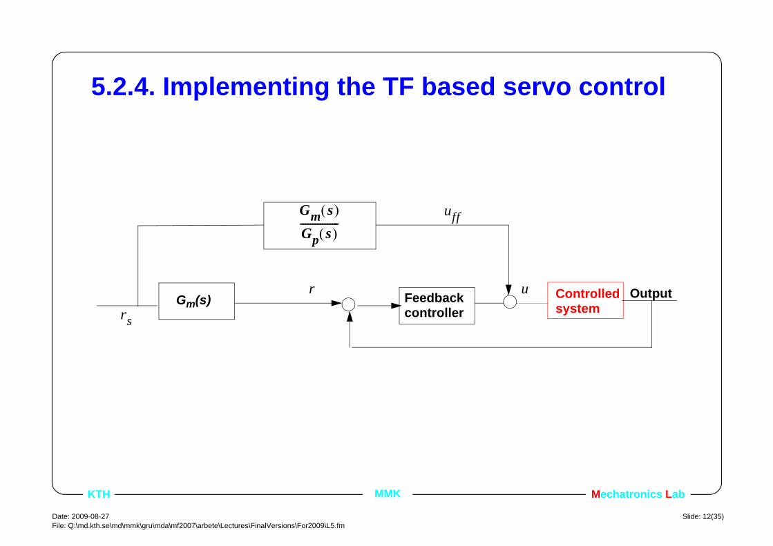
5.2.4. Implementing the TF based servo control

ControlledsystemGm(s) Output

rs

ur

uff

Feedbackcontroller

Gm s( )

Gp s( )----------------



Slide: 13(35)




• 4. An example



Slide: 14(35)


5.3.1. Model following Time domain (TD)• Instead of the combined trajectory and model following transfer function

are the trajectory and model following implemented separately

and based on trajectories in time.

• Model following: If the inverse model (from y -> u) can be written as a function of the output and n-times the derivatives of the output (n:th order model).

• Trajectory planner: Design based on closed loop

specifications and process limitations, e.g., saturation.

Gm s( )

Gp s( )---------------

u t( ) f y dydt------ d2y

dt2-------- … dny

dtn--------, , , ,

⎝ ⎠⎜ ⎟⎛ ⎞

=

y dydt------ d2y

dt2-------- … dny

dtn--------, , , ,



Slide: 15(35)

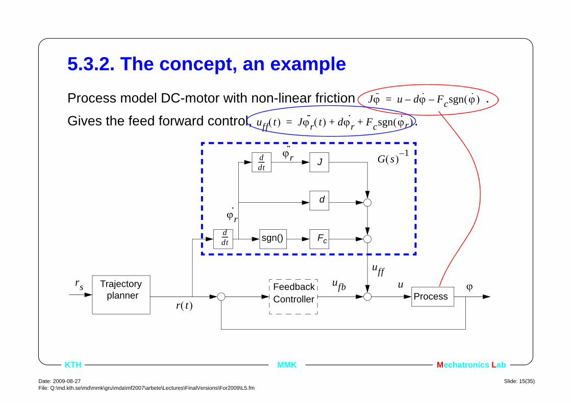
5.3.2. The concept, an exampleProcess model DC-motor with non-linear friction .

Gives the feed forward control, .

Jϕ·· u dϕ·– Fcsgn ϕ·( )–=

uff t( ) Jϕr·· t( ) dϕr

· Fcsgn ϕ· r( )+ +=

d

Fc

Trajectoryplanner Process

G s( ) 1–

sgn()

FeedbackController

rs

r t( )

uuff

ufb ϕ

J

ddt-----

ddt-----

ϕr··

ϕr·


Slide: 16(35)


5.3.3. Practical implementation• We want to avoid to take the derivative of signals.

-> The Trajectory planner must provide the derivatives

d

Fc

Trajectoryplanner

Process

G s( ) 1–

sgn()

FeedbackController

rsr ϕr= u

uffufb ϕ

J

ϕ· r

ϕ·· r



Slide: 17(35)

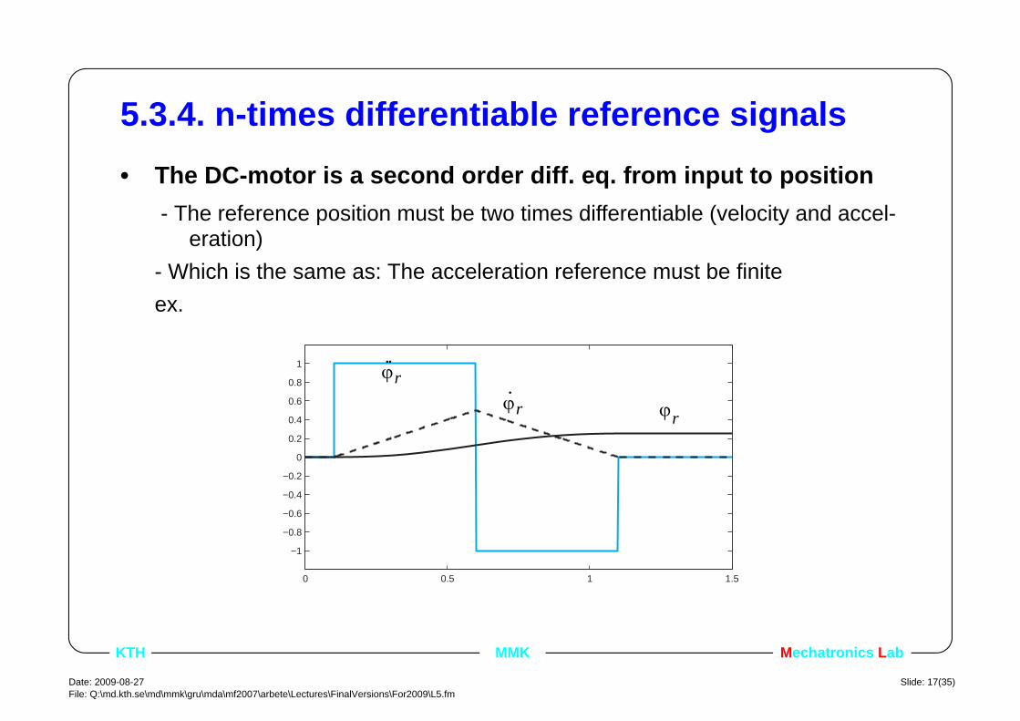
5.3.4. n-times differentiable reference signals• The DC-motor is a second order diff. eq. from input to position

- The reference position must be two times differentiable (velocity and accel-eration)

- Which is the same as: The acceleration reference must be finiteex.

0 0.5 1 1.5

−1

−0.8

−0.6

−0.4

−0.2

0

0.2

0.4

0.6

0.8

1 ϕ·· rϕ· r ϕr


Slide: 18(35)


5.3.5. How to choose the reference signals• Fastest possible positioning (or specific time trajectories)

- Calculate max acceleration and velocity of the process, without saturating the input to the motor.

- For the DC-motor: If max input torque is then max acceleration at zero velocity is . Max velocity at zero acceleration is

Mmax±

amax Mmax±( ) J⁄=

vmax Msat±( ) d Fc+( )⁄=

0 0.5 1 1.5 2 2.5

−1

−0.8

−0.6

−0.4

−0.2

0

0.2

0.4

0.6

0.8

1 rposvmax

amax

Examplereferencetrajectories



Slide: 19(35)

5.3.6. Example: how to calculate the ref. traj., zero initial condition!

, the time when maximum velocity is reached using maximum acceleration

, position reached at time

-> is the latest time to start braking.

v at=

t1vmaxamax------------=

y t1( ) amax t td

0

t1

∫12---amaxt1

2 12---

vmax2

amax------------= = = t1

rs 2y t1( )– vmax t2 t1–( )= t2rs

vmax------------

vmaxamax------------– t1+=

0 0.2 0.4 0.6 0.8 1 1.2 1.4 1.6 1.8 2−80

−60

−40

−20

0

20

40

60

80

t2

t1

Example::

rs 60vmax

,55

amax 70

===


Slide: 20(35)


5.3.7. General remarks• The two concepts of servo control are often combined

• Some process models are inherently difficult to invert.- Flexible links: Approximate the flexible model with a stiff model, the inertia and

the friction of the process is still fed forward.

• You need some margin to the theoretical maximum acceleration and speeds.- delays in computer implementation, flexibility.- Maximum torque is a function of motor speed.



Slide: 21(35)




• 4. An example



Slide: 22(35)


5.4.1. Model following control example I• Consider a second order motion control system. The output is position.

The electrical motor (the coil inductance is neglected) is operating against a linear spring with spring constant K

• Or in transfer function form

x·0 1KfJ-----–

Kemk Km⋅

J-------------------------⟨ ⟩–

0KmJ

--------u⋅+= y 1 0

x1x2

⋅=

Gp s( )Km J⁄

s2 sKm Kemk⋅

J-------------------------⎝ ⎠⎛ ⎞ Kf

J-----+ +

----------------------------------------------------------=



Slide: 23(35)

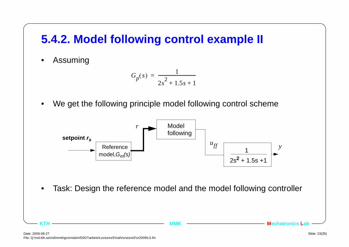
5.4.2. Model following control example II• Assuming

• We get the following principle model following control scheme

• Task: Design the reference model and the model following controller

Gp s( ) 1

2s2 1.5s 1+ +----------------------------------=

12s2 + 1.5s +1

Reference

Modelfollowing

model,Gm(s)

uff

r

ysetpoint rs


Slide: 24(35)


5.4.3. Implementing the model following• The perfect model following is the inverse of the model

(not proper)

• Use a reference model with pole excess dm > 2 (version 1)

(proper)

• Or use a trajectory planner, position, velocity and acceleration (version 2)

Gm s( ) 1=

Gm s( )

Gp s( )---------------

uff s( )

rs s( )-------------- 2s2 15s 1+ +

1---------------------------------= =

Gm s( ) ω2 s2 2ξωs ω2+ +( )⁄=

uff s( )

rs s( )-------------- 2s2 15s 1+ +( )ω2

s2 2ξωs ω2+ +---------------------------------------------=

uff s( ) 2s2 15s 1+ +( )rs s( )=

uff t( ) 2rs·· t( ) 15rs

· t( ) rs t( )+ +=



Slide: 25(35)

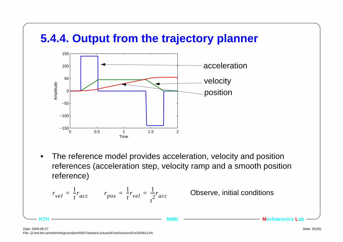
5.4.4. Output from the trajectory planner

• The reference model provides acceleration, velocity and position references (acceleration step, velocity ramp and a smooth position reference)

Observe, initial conditions

0 0.5 1 1.5 2−150

−100

−50

0

50

100

150

Time

Am

plitu

de

acceleration

velocityposition

rvel1t---racc= rpos

1t---rvel

1

t2----racc= =


Slide: 26(35)


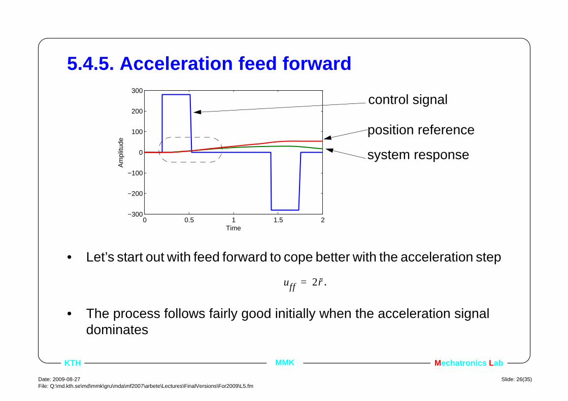
5.4.5. Acceleration feed forward

• Let’s start out with feed forward to cope better with the acceleration step

.

• The process follows fairly good initially when the acceleration signal dominates

0 0.5 1 1.5 2−300

−200

−100

0

100

200

300

Time

Am

plitu

de

control signal

system response

position reference

uff 2r··=



Slide: 27(35)

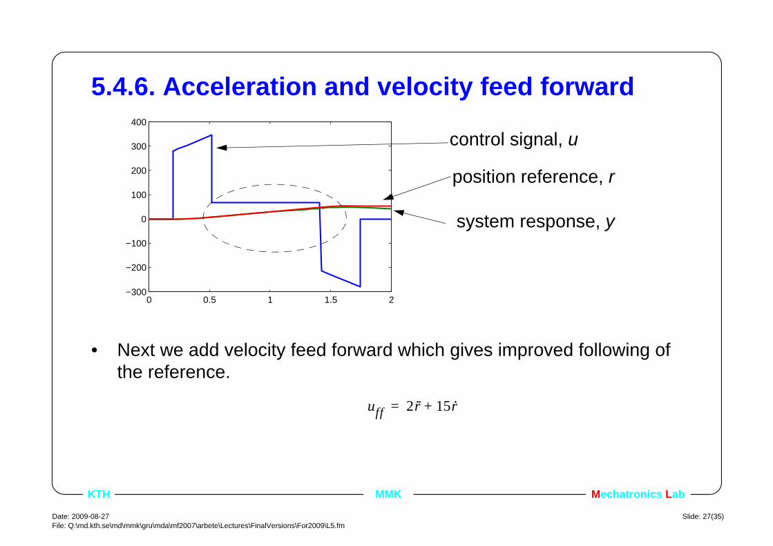
5.4.6. Acceleration and velocity feed forward

• Next we add velocity feed forward which gives improved following of the reference.

0 0.5 1 1.5 2−300

−200

−100

0

100

200

300

400

control signal, u

system response, y

position reference, r

uff 2r·· 15r·+=


Slide: 28(35)


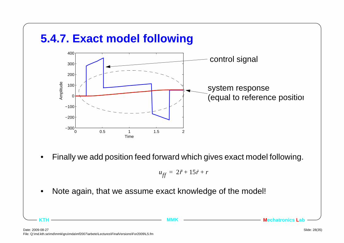
5.4.7. Exact model following

• Finally we add position feed forward which gives exact model following.

• Note again, that we assume exact knowledge of the model!

0 0.5 1 1.5 2−300

−200

−100

0

100

200

300

400

Time

Am

plitu

decontrol signal

system response(equal to reference position

uff 2r·· 15r· r+ +=



Slide: 29(35)

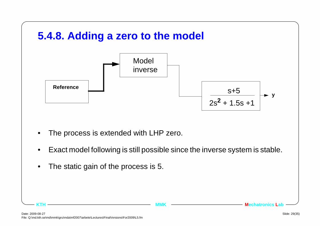
5.4.8. Adding a zero to the model

• The process is extended with LHP zero.

• Exact model following is still possible since the inverse system is stable.

• The static gain of the process is 5.

s+52s2 + 1.5s +1

yReference

Modelinverse


Slide: 30(35)


5.4.9. Feed forward without numerator inverse

• Let’s first have look on the response with only changing the gain of the feed forward controller. .

• The added dynamics (model zeros) is clearly visible.

0 0.5 1 1.5 2−60

−40

−20

0

20

40

60

80

Time

Am

plitu

decontrol signal

reference position

system response

uff2r·· 15r· r+ +

5-----------------------------=



Slide: 31(35)

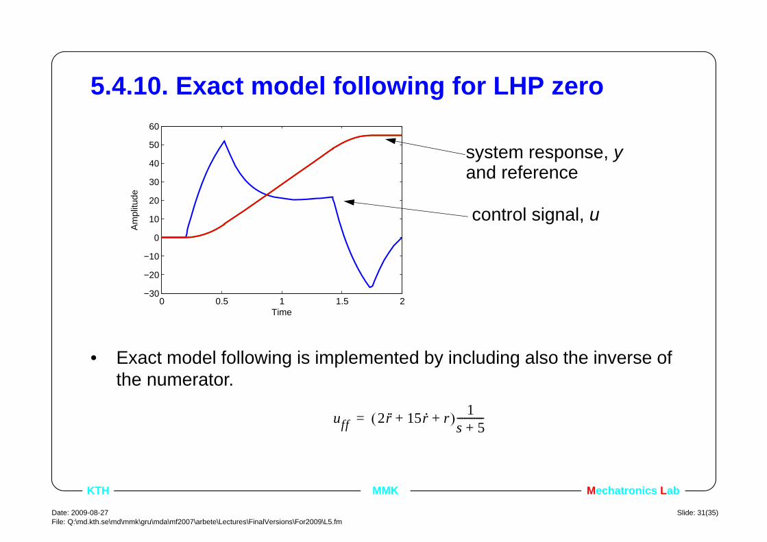
5.4.10. Exact model following for LHP zero

• Exact model following is implemented by including also the inverse of the numerator.

0 0.5 1 1.5 2−30

−20

−10

0

10

20

30

40

50

60

Time

Am

plitu

de

control signal, u

system response, yand reference

uff 2r·· 15r· r+ +( ) 1s 5+-----------=


Slide: 32(35)


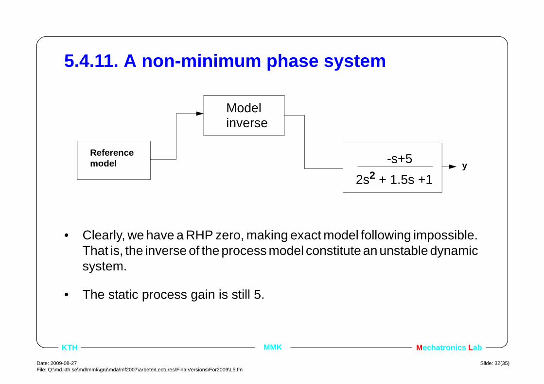
5.4.11. A non-minimum phase system

• Clearly, we have a RHP zero, making exact model following impossible. That is, the inverse of the process model constitute an unstable dynamic system.

• The static process gain is still 5.

-s+52s2 + 1.5s +1

yReferencemodel

Modelinverse



Slide: 33(35)

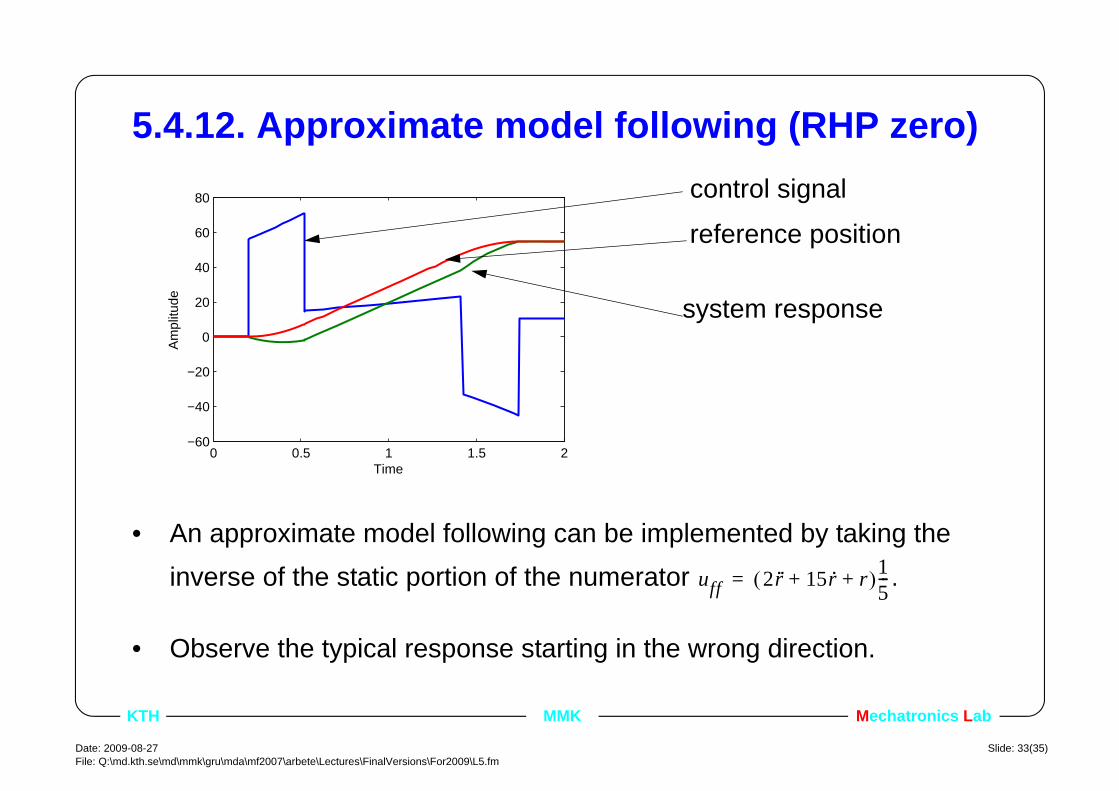
5.4.12. Approximate model following (RHP zero)

• An approximate model following can be implemented by taking the inverse of the static portion of the numerator .

• Observe the typical response starting in the wrong direction.

0 0.5 1 1.5 2−60

−40

−20

0

20

40

60

80

Time

Am

plitu

de

control signal

system response

reference position

uff 2r·· 15r· r+ +( )15---=


Slide: 34(35)


5.4.13. Summary

Controlledsystem


Trajectoryplanner

Output

SR---

Reference

Setpoint

uc

yrs

Control u

Controluff

Design the trajectory planner based on the performance of the motor.

Design the model following control based on an inverse model of the process. Excellent for non-linear phenomena.



Slide: 35(35)




• 4. An example


Documents

Dynamics and motion control Lecture 5 Model following ... · KTH MMK Mechatronics Lab 5.3.7. General remarks • The two concepts of servo control are often combined • Some process