Dynamics and Controls Modeling and Analysis Toolbox (DOCS

1

MIT Space Systems LaboratoryChart: 1September 22, 2000

Interferometry Summer School, Leiden NL

Interferometry Summer SchoolInterferometry Summer School18-22 September 2000, Leiden,NL18-22 September 2000, Leiden,NL

Dynamics and Controls Modeling andDynamics and Controls Modeling andAnalysis Toolbox (DOCS) forAnalysis Toolbox (DOCS) forSpace-Based ObservatoriesSpace-Based Observatories

Olivier de Weck, Prof. David MillerOlivier de Weck, Prof. David MillerSpace Systems LaboratorySpace Systems Laboratory

Massachusetts Institute of TechnologyMassachusetts Institute of [email protected]@mit.edu

Abstract

The DOCS (Dynamics-Optics-Controls-Structures) framework presented hereis a powerful toolbox for the modeling and analysis of precision opto-mechanical systems such as interferometers. Within the MATLABenvironment a model of the system can be created, which simulates thedynamic behavior of the structure, the optical train, the control systems and theexpected disturbance sources in an integrated fashion. This modeling is criticalin order to identify important modal and physical parameters of the systemthat drive the opto-mechanical performance. Other uses are the developmentand tuning of attitude and optical controllers, uncertainty analysis, modelupdating with test data, the development of error budgets and the flowdown ofsubsystem requirements. This presentation outlines the technical challengesfaced by precision telescopes and gives an overview of how the DOCSframework can assist in solving observatory design problems. Two specificanalysis examples are presented. First the derivation of an error budget forNGST with two performance metrics and three error sources is shown.Secondly the effect of reaction wheel disturbances and OPD control bandwidthon the transmissivity function of TPF is presented. Experimental validations ofthe toolbox are carried out with telescope testbeds in 1g. Preliminary versionsof the framework have been successfully applied to conceptual designs ofSIM, NGST, TPF and Nexus.

2



Technological Challenges

HST - 1990

NEXUS-2004 SIM-2006NGST-2009

Deployable Cold OpticsNGST Precursor Mission

Faint Star InterferometerPrecision Astrometry

Lightweight 8m-OpticsIR Deep Field Observations

Space-Based ObservatoryMultipurpose UV/Visual/IR Imaging and Spectroscopy

The next generation of space based observatories isexpected to provide significant improvements in

angular resolution, spectral resolution and sensitivity.

ScienceRequirements

EngineeringRequirements

D&C SystemRequirements

TPF-2011

5 year wide-angle astro-metric accuracy of 4 µµasec

to limit 20th Magnitude stars

Fringe Visibility> 0.8 for astrometry

Science InterferometerOPD < 10 nm RMS

Sample Requirements Flowdown for SIM

Achieve requirements in a cost-effective manner with predictable risk level.

Nulling InterferometerPlanet Detection

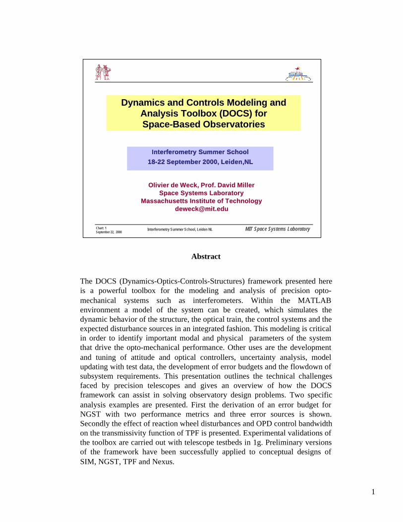
The Hubble Space Telescope (HST) has celebrated it’s 10th year of on-orbitoperation in 2000. Hubble has broken technological ground for space basedastronomy as a multi-purpose UV/visual and IR observatory. The main scienceobjectives for Hubble are multi-purpose astrophysical imaging andspectroscopy. The next generation of space based observatories, includinginterferometers is being designed at this time and is expected to providesignificant improvements in angular resolution, spectral resolution andsensitivity. In spaceborne interferometry SIM will provide precisionastrometry for faint stars and TPF (and DARWIN) will work as a nulling(Bracewell) interferometer for direct plant detection in the IR. In designingthese ambitious missions a requirements flowdown is taking place from thescience requirements, to the engineering requirements to sub-disciplinerequirements such as dynamics and controls (D&C). Thus phasing andpointing requirements for the metrology-, guide- and science-light can bepostulated in terms of wavefront error (WFE), optical pathlength difference(OPD), wavefront tilt (WFT), line-of-sight(LOS) jitter, beam shear (BS) andothers. The primary objective of DOCS is to address these dynamic systemrequirements. This can be done for the various telescope modes such asscience light integration, tracking, retargeting and slewing.

3



Research Motivation - Problem Statement

Disturbances

Opto-Structural Plant

White Noise Input

Control

Performances

Phasing (WFE)

Pointing (LOS)

σσz,2 = RSS LOS

Appended LTI System Dynamics

(ACS, FSM, ODL)

(RWA, Cryo)

d

w

u y

z

ΣΣ ΣΣActuator Noise Sensor

Noise

σσz,1=RMS WFE

[Ad,Bd,Cd,Dd]

[Ac ,Bc ,Cc,Dc]

OverallState Vector

plantstates

disturbancestates

controllerstates

qd

qpqc

qzd=[Az d, Bzd, Cz d, Dzd]

z=Czd qz d

Science Target Observation Mode

# of parameters: j=1…n p# of performances: i=1…nz

np>nz

Parameters: pj

Video Clip

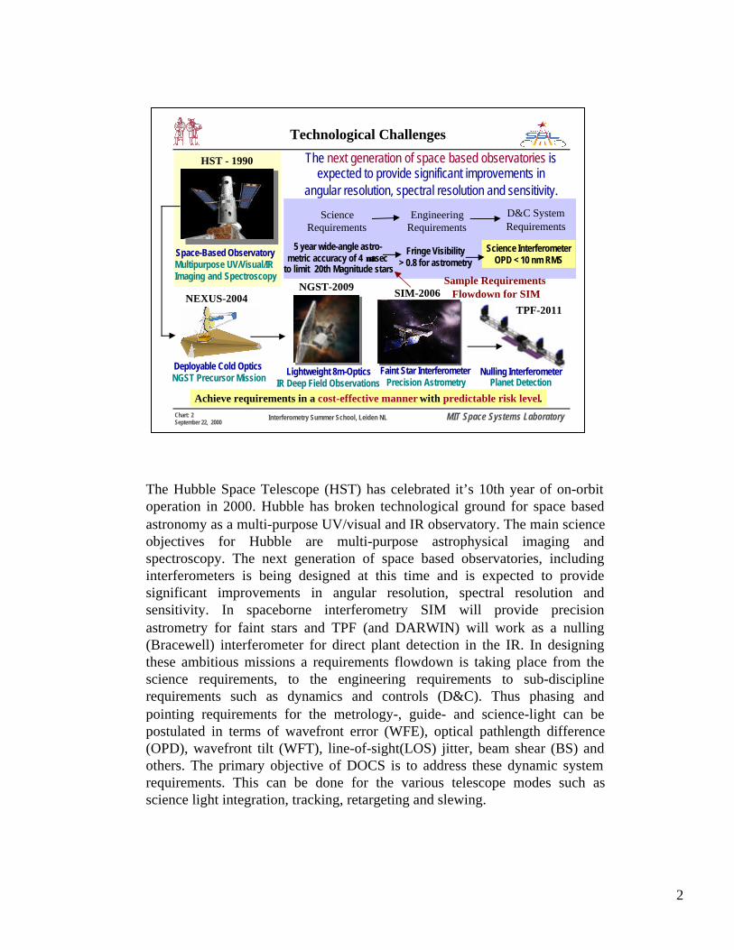
The present work is motivated by the need to simulate the dynamic behavior ofthe future generation of space interferometers during the conceptual andpreliminary design phases. In order for these space or ground-based telescopesto meet their stringent phasing (e.g. OPD) and pointing requirements (e.g. LOSjitter), the path from disturbances to the performance metrics of interest ,z ,must be modeled in detail. It is assumed that the systems are linear and time-invariant (LTI). The premise is that a number of disturbances sources (reactionwheel assembly (RWA), cryocooler, guide star noise etc.) are acting during thevarious operational modes of interest as zero-mean random stochasticprocesses. Their effect is captured with the help of state space shaping filters[Ad,Bd,Cd,Dd], such that the input to the appended system dynamics[Azd,Bzd,Czd,Dzd] is assumed to be unit-intensity white noise d, which isuncorrelated for each disturbance source. The shaped disturbances w arepropagated through the opto-structural plant dynamics [Ap,Bp,Cp,Dp], whichinclude the structural dynamics of the spacecraft and the linear optics matrices.A compensator [Ac,Bc,Cc,Dc] is often present in order to stabilize theobservable rigid body modes (ACS) and to improve the disturbance rejectioncapability (ODL, FSM). The sensor outputs y and actuator inputs u might besubject to noise. One of the goals of the DOCS framework is to accuratelypredict the root-mean-square (RMS) values and sensitivities of theperformances z under the above assumptions.Reaction Wheel Picture: http://www.ithaco.com/T-Wheel.html, FSM picture:http://www.lefthand.com/prod_fsm.html, SIM Picture: http://sim.jpl.nasa.gov

4



Examples

DOCS Toolbox Structure

Design Structure:IMOSStructure:IMOS

DisturbanceSources

DisturbanceSources

DYNAMODDYNAMOD

UncertaintyDatabase

UncertaintyDatabase

Baseline Control

Baseline Control

Model Reduction &Conditioning

Model Reduction &Conditioning

ModelAssembly

ModelAssembly

ModelUpdating

ModelUpdating

DisturbanceAnalysis

DisturbanceAnalysis

Sensor &Actuator

Topologies

Sensor &Actuator

Topologies

UncertaintyAnalysis

UncertaintyAnalysis

ControlForgeControlForge

Data

SystemControlStrategy

Modeling Model Prep Analysis Design

CampbellBourgault

Gutierrez

Mallory

Masterson

Moore Skelton

Jacques

ControlTuning

ControlTuning

Optics:MACOSOptics:MACOS

Hasselman

IsoperformanceIsoperformance

SubsystemRequirements

ErrorBudgets

Blaurock

JPL

ZhouHowHall

Miller

Balmes

Blaurock

OptimizationOptimization

SensitivitySensitivity

ΣΣ Margins

MastersCrawley

Haftka

Gutierrez

System Requirements

Feron

Feron

van Schoor

Crawley

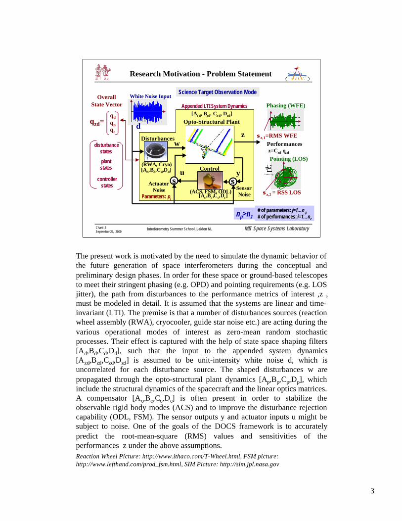
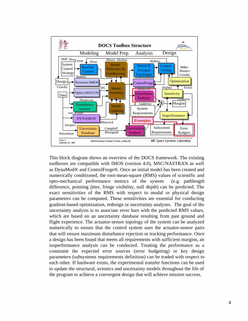
This block diagram shows an overview of the DOCS framework. The existingtoolboxes are compatible with IMOS (version 4.0), MSC/NASTRAN as wellas DynaMod® and ControlForge®. Once an initial model has been created andnumerically conditioned, the root-mean-square (RMS) values of scientific andopto-mechanical performance metrics of the system (e.g. pathlengthdifference, pointing jitter, fringe visibility, null depth) can be predicted. Theexact sensitivities of the RMS with respect to modal or physical designparameters can be computed. These sensitivities are essential for conductinggradient-based optimization, redesign or uncertainty analyses. The goal of theuncertainty analysis is to associate error bars with the predicted RMS values,which are based on an uncertainty database resulting from past ground andflight experience. The actuator-sensor topology of the system can be analyzednumerically to ensure that the control system uses the actuator-sensor pairsthat will ensure maximum disturbance rejection or tracking performance. Oncea design has been found that meets all requirements with sufficient margins, anisoperformance analysis can be conducted. Treating the performance as aconstraint the expected error sources (error budgeting) or key designparameters (subsystems requirements definition) can be traded with respect toeach other. If hardware exists, the experimental transfer functions can be usedto update the structural, avionics and uncertainty models throughout the life ofthe program to achieve a convergent design that will achieve mission success.

5



Example 1: Error Budgeting (I)

(1) Why is error budgeting important ?

(2) How is it done today?

(3) How can DOCS/ isoperformance help error budgeting ?

Goal: Balance anticipated error sources, which are given by physical process limits and imperfections of hardware in a predictable and physically realizable

manner. Example: balancing of sensor vs. process noise.NGST Example : Assume 3 Main Error Sources

Error Source 2: RWA Error Source 3: GS Noise

Us: Static Imbalance [gcm] Tint: Integration Time [sec]0.005 <= Qc <= 0.05

Error Source 1: CRYO

Qc: Amplification Factor [-]0 0.5 1

-2

0

2 Axial Force [N]

[sec] 0 1 2 3 4 5 6 7 8-5

-4

-3

-2

-1

0

1

2

3

4

5x 10

-3

Time [sec]x

RWA Force Fx

1.0 <= U s <= 30.0 0.020 <= Tint <= 0.100

-0.04 -0.03 -0.02 -0.01 0 0.01 0.02 0.03 0.04-0.04

-0.03

-0.02

-0.01

0

0.01

0.02

0.03

Centroid Pos

Establishes feasibility of dynamic systemperformance given noise source assumptions.

Ad-Hoc error budgeting, RSS error tree,limited physical understanding of interactions.

Leverages sensitivity analysis and integrated modeling. Creates link to physical parameters .

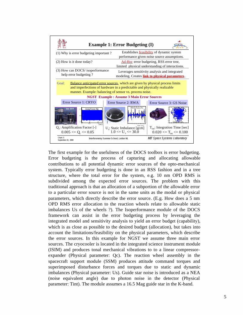
The first example for the usefulness of the DOCS toolbox is error budgeting.Error budgeting is the process of capturing and allocating allowablecontributions to all potential dynamic error sources of the opto-mechanicalsystem. Typically error budgeting is done in an RSS fashion and in a treestructure, where the total error for the system, e.g. 10 nm OPD RMS issubdivided among the expected error sources. The problem with thistraditional approach is that an allocation of a subportion of the allowable errorto a particular error source is not in the same units as the modal or physicalparameters, which directly describe the error source. (E.g. How does a 5 nmOPD RMS error allocation to the reaction wheels relate to allowable staticimbalances Us of the wheels ?). The Isoperformance module of the DOCSframework can assist in the error budgeting process by leveraging theintegrated model and sensitivity analysis to yield an error budget (capability),which is as close as possible to the desired budget (allocation), but takes intoaccount the limitations/feasibility on the physical parameters, which describethe error sources. In this example for NGST we assume three main errorsources. The cryocooler is located in the integrated science instrument module(ISIM) and produces tonal mechanical vibrations to to a linear compressor-expander (Physical parameter: Qc). The reaction wheel assembly in thespacecraft support module (SSM) produces attitude command torques andsuperimposed disturbance forces and torques due to static and dynamicimbalances (Physical parameter: Us). Guide star noise is introduced as a NEA(noise equivalent angle) due to photon noise in the detector (Physicalparameter: Tint). The module assumes a 16.5 Mag guide star in the K-band.

6



Example 1: Error Budgeting (II)

ERROR SOURCE 1

ERROR SOURCE 2ERROR SOURCE 3

PERFORMANCE 1

PERFORMANCE 2

-K-

ps-1

ps

ps

nm

nm

-K-

mean

XY Graph

White Noise

Ch X

WhiteNoise

RWA

WhiteNoiseCryo

WhiteNoiseCh Y

x' = Ax+Bu y = Cx+Du

SpacecraftStructuralDynamics

Scope

Mux

Mux

Mux

MuxsqrtMath

Function1

sqrt

MathFunction

t_losLOS Jitter

K

Kwfe

K

Klos

K KfsmK

Kacs


HexapodIsolator


FSM Controller


FGSNoise

t_wfeDynamic WFE

Dot Product2

Dot Product

Demux

Demux


CryocoolerDisturbance


AttitudeControl System


Reaction Wheel Assembly Disturbance

Dynamics and Controls Block Diagram for NGST

486 states

Disturbance Parameters(Inhomogeneous Dynamics)

Plant Parameters(Homogeneous Dynamics)

Control Parameters(Homogeneous Dynamics)

(variable) (fixed) (fixed)

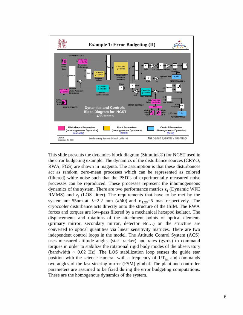
This slide presents the dynamics block diagram (Simulink®) for NGST used inthe error budgeting example. The dynamics of the disturbance sources (CRYO,RWA, FGS) are shown in magenta. The assumption is that these disturbancesact as random, zero-mean processes which can be represented as colored(filtered) white noise such that the PSD’s of experimentally measured noiseprocesses can be reproduced. These processes represent the inhomogeneousdynamics of the system. There are two performance metrics z1 (Dynamic WFERMMS) and z2 (LOS Jitter). The requirements that have to be met by thesystem are 55nm at λ=2.2 mm (λ/40) and σLOS=5 mas respectively. Thecryocooler disturbance acts directly onto the structure of the ISIM. The RWAforces and torques are low-pass filtered by a mechanical hexapod isolator. Thedisplacements and rotations of the attachment points of optical elements(primary mirror, secondary mirror, detector etc…) on the structure areconverted to optical quantities via linear sensitivity matrices. There are twoindependent control loops in the model. The Attitude Control System (ACS)uses measured attitude angles (star tracker) and rates (gyros) to commandtorques in order to stabilize the rotational rigid body modes of the observatory(bandwidth ~ 0.02 Hz). The LOS stabilization loop senses the guide starposition with the science camera with a frequency of 1/T int and commandstwo angles of the fast steering mirror (FSM) gimbal. The plant and controllerparameters are assumed to be fixed during the error budgeting computations.These are the homogenous dynamics of the system.

7



Example 1: Error Budgeting (III)

Isoperformance Engine

Example: NGST Error Budget (Excel)

Find Error SourceContributions

EvaluateError Contribution

Sphere

Cap

abili

ty =

Clo

sest

Fea

sib

le E

rro

r B

ud

get

LTI System , σσz,req,p_bounds, p_nom

Isoperformancesolution set

Parameters: Qc=0.029, Us=14.09, Tint=0.0407

0.20.4

0.60.8

00.2

0.40.6

0.8

0

0.2

0.4

0.6

0.8

CRYO

Error Contribution

Sphere

RWA

GS

Noi

se

WFE BudgetLOS BudgetCapability

var_contr

z1: WFE RMS [nm] Req: 55.00 z2: LOS Jitter [asec] Req: 0.005Error Source VAR % Allocation VAR% Capability VAR % Allocation VAR% CapabilityCryocooler 0.49 38.50 0.72 46.6467 0.40 0.003162 0.31 0.002823RWA 0.49 38.50 0.28 29.1543 0.40 0.003162 0.53 0.0037016GStar Noise 0.02 7.78 0.00 0.0000 0.20 0.002236 0.17 0.0020829Total 55.00 55.0081 0.005000 0.0051

1.0

Allo

cate

d B

ud

get

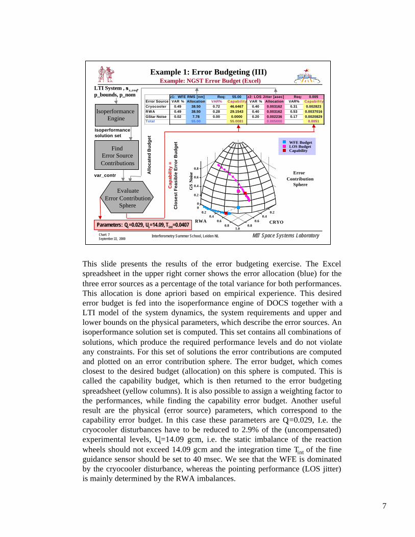
This slide presents the results of the error budgeting exercise. The Excelspreadsheet in the upper right corner shows the error allocation (blue) for thethree error sources as a percentage of the total variance for both performances.This allocation is done apriori based on empirical experience. This desirederror budget is fed into the isoperformance engine of DOCS together with aLTI model of the system dynamics, the system requirements and upper andlower bounds on the physical parameters, which describe the error sources. Anisoperformance solution set is computed. This set contains all combinations ofsolutions, which produce the required performance levels and do not violateany constraints. For this set of solutions the error contributions are computedand plotted on an error contribution sphere. The error budget, which comesclosest to the desired budget (allocation) on this sphere is computed. This iscalled the capability budget, which is then returned to the error budgetingspreadsheet (yellow columns). It is also possible to assign a weighting factor tothe performances, while finding the capability error budget. Another usefulresult are the physical (error source) parameters, which correspond to thecapability error budget. In this case these parameters are Qc=0.029, I.e. thecryocooler disturbances have to be reduced to 2.9% of the (uncompensated)experimental levels, Us=14.09 gcm, i.e. the static imbalance of the reactionwheels should not exceed 14.09 gcm and the integration time Tint of the fineguidance sensor should be set to 40 msec. We see that the WFE is dominatedby the cryocooler disturbance, whereas the pointing performance (LOS jitter)is mainly determined by the RWA imbalances.

8



Example 2: RWA Noise and Nulling Performance

No

rmal

ized

In

ten

sity

Angular separation in sky

0.5 AU

Interferometer Transmissivity Function

Reaction wheel imbalances causevibrations that “wash out”

lobes in the transmissivity functionExample: ITHACO E-Wheel

Wheel speed 1000 +/- 1000 RPMSymmetric Pyramid of 4 Wheels

Nominal Test data : Scale factor =1.0 Increased Imbalances : Scale factor =10.0

SF=10SF=1

“Washout” Effect

TPF

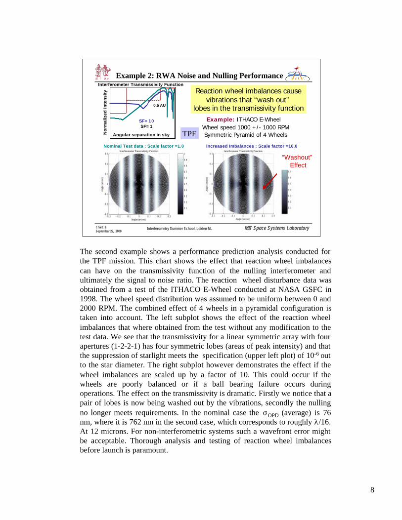
The second example shows a performance prediction analysis conducted forthe TPF mission. This chart shows the effect that reaction wheel imbalancescan have on the transmissivity function of the nulling interferometer andultimately the signal to noise ratio. The reaction wheel disturbance data wasobtained from a test of the ITHACO E-Wheel conducted at NASA GSFC in1998. The wheel speed distribution was assumed to be uniform between 0 and2000 RPM. The combined effect of 4 wheels in a pyramidal configuration istaken into account. The left subplot shows the effect of the reaction wheelimbalances that where obtained from the test without any modification to thetest data. We see that the transmissivity for a linear symmetric array with fourapertures (1-2-2-1) has four symmetric lobes (areas of peak intensity) and thatthe suppression of starlight meets the specification (upper left plot) of 10-6 outto the star diameter. The right subplot however demonstrates the effect if thewheel imbalances are scaled up by a factor of 10. This could occur if thewheels are poorly balanced or if a ball bearing failure occurs duringoperations. The effect on the transmissivity is dramatic. Firstly we notice that apair of lobes is now being washed out by the vibrations, secondly the nullingno longer meets requirements. In the nominal case the σOPD (average) is 76nm, where it is 762 nm in the second case, which corresponds to roughly λ/16.At 12 microns. For non-interferometric systems such a wavefront error mightbe acceptable. Thorough analysis and testing of reaction wheel imbalancesbefore launch is paramount.

9



10

Optical Control System improves nulling performance

Trade studyshows that

optical controlbandwidth

is insufficientat 5 Hz but

can meet therequirements

at 100 Hz

10-4

10-3

10-2

10-110

-12

10-10

10-8

10-6

10-4

10-2

100

Nor

mal

ized

Inte

nsity

Angular separation in sky (arcsec)

0.5 AU

Exo-solar systemat 10 pc

Interferometer Transmissivity Function

5 Hz Optical Control BW100 Hz Optical Control BW

σOPD=27.3 nm

σOPD=107 nm

Note: RMS OPD values shown are average for

all apertures

Requirement

4 Apertures, SCI,linear symmetric @ 1AU

Example 2: Effect of Optical Control on Nulling

TPF

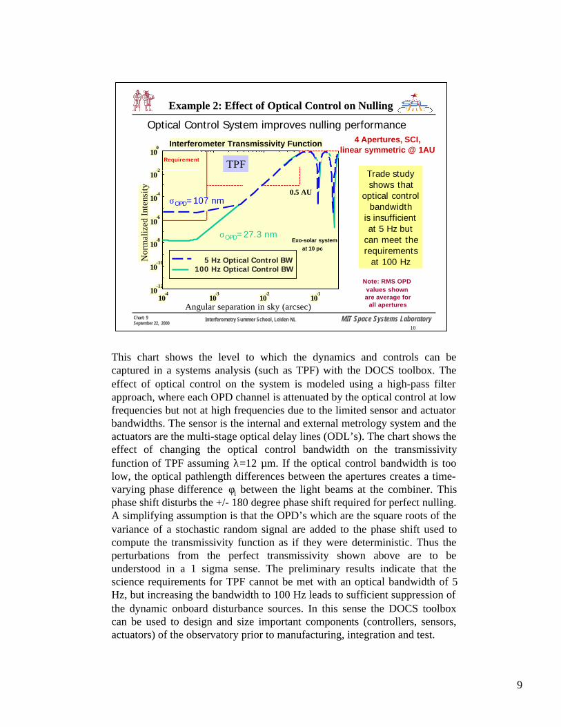
This chart shows the level to which the dynamics and controls can becaptured in a systems analysis (such as TPF) with the DOCS toolbox. Theeffect of optical control on the system is modeled using a high-pass filterapproach, where each OPD channel is attenuated by the optical control at lowfrequencies but not at high frequencies due to the limited sensor and actuatorbandwidths. The sensor is the internal and external metrology system and theactuators are the multi-stage optical delay lines (ODL’s). The chart shows theeffect of changing the optical control bandwidth on the transmissivityfunction of TPF assuming λ=12 µm. If the optical control bandwidth is toolow, the optical pathlength differences between the apertures creates a time-varying phase difference φi between the light beams at the combiner. Thisphase shift disturbs the +/- 180 degree phase shift required for perfect nulling.A simplifying assumption is that the OPD’s which are the square roots of thevariance of a stochastic random signal are added to the phase shift used tocompute the transmissivity function as if they were deterministic. Thus theperturbations from the perfect transmissivity shown above are to beunderstood in a 1 sigma sense. The preliminary results indicate that thescience requirements for TPF cannot be met with an optical bandwidth of 5Hz, but increasing the bandwidth to 100 Hz leads to sufficient suppression ofthe dynamic onboard disturbance sources. In this sense the DOCS toolboxcan be used to design and size important components (controllers, sensors,actuators) of the observatory prior to manufacturing, integration and test.

10



Experimental Validation (1)

Test Article allows to trade:imbalance Us, mass m1, Wheel Speed

Ro, Suspension Spring Stiffness k1

Reaction Wheel Disturbance Testbed

Axial Stabilization System

Weight Bed

Lower Stage

Upper Stage: RWA

Goal: Validate predictive capabilityof DOCS toolbox on a test article

050

100150

200

0

1000

2000

30000

5

10

15

20

Mass m1

[lbs]

Kistler Accelerometer Results

Wheel Speed [RPM]

Dis

plac

emen

t R

MS

[ µµm

]

050

100150

200

0

1000

2000

30000

5

10

15

20

Mass m 1 [lbs]

Performance Prediction (6 state model)

Wheel Speed [RPM]

Dis

plac

emen

t R

MS

[ µµm

]

Demo

Video Clip

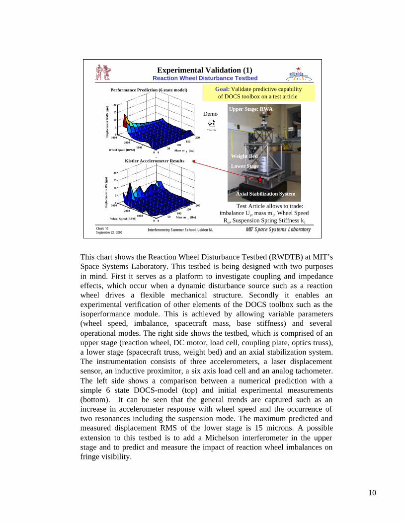
This chart shows the Reaction Wheel Disturbance Testbed (RWDTB) at MIT’sSpace Systems Laboratory. This testbed is being designed with two purposesin mind. First it serves as a platform to investigate coupling and impedanceeffects, which occur when a dynamic disturbance source such as a reactionwheel drives a flexible mechanical structure. Secondly it enables anexperimental verification of other elements of the DOCS toolbox such as theisoperformance module. This is achieved by allowing variable parameters(wheel speed, imbalance, spacecraft mass, base stiffness) and severaloperational modes. The right side shows the testbed, which is comprised of anupper stage (reaction wheel, DC motor, load cell, coupling plate, optics truss),a lower stage (spacecraft truss, weight bed) and an axial stabilization system.The instrumentation consists of three accelerometers, a laser displacementsensor, an inductive proximitor, a six axis load cell and an analog tachometer.The left side shows a comparison between a numerical prediction with asimple 6 state DOCS-model (top) and initial experimental measurements(bottom). It can be seen that the general trends are captured such as anincrease in accelerometer response with wheel speed and the occurrence oftwo resonances including the suspension mode. The maximum predicted andmeasured displacement RMS of the lower stage is 15 microns. A possibleextension to this testbed is to add a Michelson interferometer in the upperstage and to predict and measure the impact of reaction wheel imbalances onfringe visibility.

11



2

1

Experimental Validation (2)ORIGINS Telescope Testbed

ActuatorsRWA Reaction Wheel AssemblyVC Voice Coil MirrorPZT Piezo MirrorFSM Fast Steering Mirror

Testbed Transfer Functions

SensorsENC Digital Angle EncoderRGA Rate Gyro AssemblyDPL Differential Path LaserQC Quad Cell Pointing

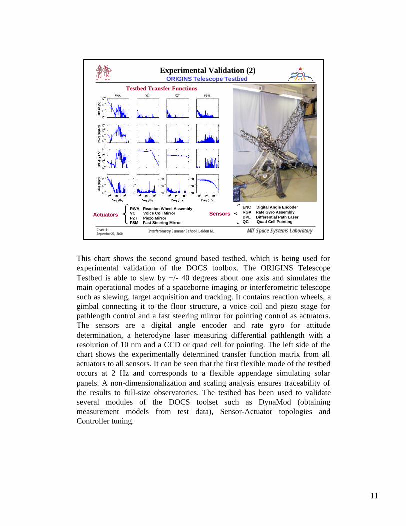
This chart shows the second ground based testbed, which is being used forexperimental validation of the DOCS toolbox. The ORIGINS TelescopeTestbed is able to slew by +/- 40 degrees about one axis and simulates themain operational modes of a spaceborne imaging or interferometric telescopesuch as slewing, target acquisition and tracking. It contains reaction wheels, agimbal connecting it to the floor structure, a voice coil and piezo stage forpathlength control and a fast steering mirror for pointing control as actuators.The sensors are a digital angle encoder and rate gyro for attitudedetermination, a heterodyne laser measuring differential pathlength with aresolution of 10 nm and a CCD or quad cell for pointing. The left side of thechart shows the experimentally determined transfer function matrix from allactuators to all sensors. It can be seen that the first flexible mode of the testbedoccurs at 2 Hz and corresponds to a flexible appendage simulating solarpanels. A non-dimensionalization and scaling analysis ensures traceability ofthe results to full-size observatories. The testbed has been used to validateseveral modules of the DOCS toolset such as DynaMod (obtainingmeasurement models from test data), Sensor-Actuator topologies andController tuning.

12



Conclusions

Further information contact: [email protected]

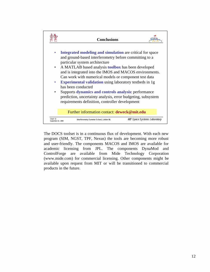
• Integrated modeling and simulation are critical for spaceand ground-based interferometry before committing to aparticular system architecture

• A MATLAB based analysis toolbox has been developedand is integrated into the IMOS and MACOS environments.Can work with numerical models or component test data

• Experimental validation using laboratory testbeds in 1ghas been conducted

• Supports dynamics and controls analysis: performanceprediction, uncertainty analysis, error budgeting, subsystemrequirements definition, controller development

The DOCS toolset is in a continuous flux of development. With each newprogram (SIM, NGST, TPF, Nexus) the tools are becoming more robustand user-friendly. The components MACOS and IMOS are available foracademic licensing from JPL. The components DynaMod andControlForge are available from Mide Technology Corporation(www.mide.com) for commercial licensing. Other components might beavailable upon request from MIT or will be transitioned to commercialproducts in the future.

Documents

Dynamics and Controls Modeling and Analysis Toolbox (DOCS