DYNAMICAL THEORY OF NEUTRON DIFFRACTION FOR PERFECT

CRYSTALS WITH AND WITHOUT STRAIN GRADIENTS

Saravanamuthu Maheswaran

B.Sc.(Physics Honours), University of Peradeniya, Sri Lanka, 1981

M.Sc.(Bio Physics), Simon Fraser University, 1985

A THESIS SUBMITTED IN PARTIAL FULFILLMENT OF

THE REQUIREMENTS FOR THE DEGREE OF

DOCTOR OF PHILOSOPHY

in the Department

of

Physics

O Saravanamuthu Maheswaran 1989

SIMON FRASER UNIVERSITY

March 1989

All rights reserved. This work may not be

reproduced in whole or in part, by photocopy

or other means, without permission of the author.

APPROVAL

Name: Saravanamuthu Maheswaran

Degree: Doctor of Philosophy

Title of Thesis: Dynamical Theory of Neutron Diffraction for Parfect Crystals with and

without Strain Gradients

Examining Committee:

Chairman: J. F. Cochran

.,- s - - . J /

A. S. Arrott

Senior Supervisor

- - L. E. Ballentine

V

A. E. Curzon

d Y

E. D. Crozier

- L- : -

- . . -.--- 7 . - S. A. Werner

External Examiner

Physics Department, University of Missouri, Columbia

Date Approved: March 17. 1989

PARTIAL COPYRIGHT LICENSE

I hereby grant t o S I m n Fraser U n i v e r s i t y the r i g h t t o lend

my thes is , proJect o r extended essay ( t h e t i t l e o f which i s shown below)

t o users o f the Simon Fraser U n i v e r s i t y L ib ra ry , and t o make p a r t i a l o r

s i n g l e copies on ly f o r such users o r I n response t o a request from the

l i b r a r y o f any o ther un i ve rs i t y , o r o t h e r educat ional I n s t i t u t i o n , on

i t s own behalf o r f o r one o f I t s users. I f u r t h e r agree t h a t permission

f o r m u l t i p l e copying o f t h i s work f o r s c h o l a r l y purposes may be granted

by me o r the Dean o f Graduate Studies. I t i s understood t h a t copying

o r publication of t h i s work f o r f i n a n c i a l ga in s h a l l not be al lowed

w i thout my w r i t t e n permission,

T i t l e o f Thes i s/Project/Extended Essay

Dynamical Theory of Neutron D i f f r a c t i o n f o r

P e r f e c t Crys t a l s With and Without S t r a i n Gradient6

. Author: y.J - v I r . w ~ - , u J u r . --- / r

(s ignature)

S. Maheswaran

( name

ABSTRACT

The dynamical theory of neutron diffraction is studied for perfect crystals and crystals

with strain gradients. In the case of parallel-sided slab crystals, it is customary to

distinguish the Bragg case where the beam enters and exits on the same side of the slab and

the Laue case where the beam enters on one side and exits on the other. The symmetric

Bragg case has the angle of incidence equal to the angle of diffraction with respect to the 1

surface, that is the scattering vector is perpendicular to the surface. In the symmetric Laue

case the scattering vector is parallel to the surface. In extreme cases either the incoming or

exiting beam is close to being parallel to the surface. Schriidinger's equation for the perfect

slab crystal with a periodic potential is solved by two methods which can give similar

results. In the first method, which is known as the eikonal approach, a quartic dispersion

relation is obtained and solved for all possible internal wave vectors. A given incident

plane wave generates four pairs of internal waves. Each pair is coupled together by the

periodic potential. Four waves, in addition to the incident wave, appear outside the crystai

as a result of the interaction with the crystal slab. All the unknown internal and external

amplitudes are found from the boundary conditions. In non-extreme cases, two pairs of

internal waves suffice to describe the propagation of neutrons in the crystal. In the second

approach, commonly referred to as the Takagi-Taupin method, one assumes that the wave

amplitudes are position dependent solutions of coupled differential equations. We have

measured the dependence of the diffracted beam intensity as a function of thickness of Si

wafers and found good agreement with the theory. The theory has applications in the

design of elements for neutron optics, particularly monochromating and analyzing crystals.

In the extreme cases, all four pairs of internal waves are considered. It is shown that

three pairs are sufficient to describe adequately the propagation of neutrons inside the

crystal in almost all cases. The treatment of perfect crystals given here is unique in the

fullness of the approach and its direct application to a simple and actual experimental

geometry.

For practical design considerations it is necessary to introduce elastic strain gradients to

improve the efficiency of elements for neutron optics. In the case of homogeneously bent

crystals, the solutions of the dynamical problem have been expressed by others in terms of

confluent hypergeometric functions. Mathematical obscurities have been eliminated here by

expressing the confluent hypergeometric functions in terms of Chebyshev polynomials.

The results are in a form suitable for numerical computation of the variation of intensity of

neutron scattering with crystal thickness and amplitude of the strain gradient. In the

experiments the crystals are bent by loading along two lines at each of two parallel edges.

The resulting strain gradients are more complicated than expected. In addition in most of

our experiments we have exceeded the limits in which the simple bending theory can be

applied. In this situation the displacement field is given by two nonlinear fourth order

differential equations. The elasticity theory of bending and the dynarnical theory of

diffraction can be computationally combined to interpret the experimental results.

Dedicated to my father

for his continual support and encozcragement.

ACKNOWLEDGEMENTS

My deepest gratitude and sincere thanks goes to my senior supervisor, Professor

Anthony Arrott, for his constant encouragement, assistance and humor during the course of

this project. His unbridled enthusiasm and continually fertile imagination were a great

source of inspiration for me to complete this project.

Special thanks also goes to Dr. T. Templeton for providing experimental results and

for many helpful discussions. I wish to thank the members of the supervisory committee

Profs. L. E. Ballentine and A. E. Curzon for their useful discussions in writing the thesis.

I also thank the external examiner Prof. S. A. Werner and the university examiner Prof. E.

D. Crozier for their many helpful suggestions.

I record my sincere thanks to my colleagues, specially, Steve Purcell, Jeff Rudd, Don

Hunter, Ken Urquhart, Ross Walker and Ken Myrtle for their kind assistance at various

instances during the study.

The financial support from my supervisor through a research grant from the Natural

Sciences and Engineering Research Council of Canada, the scholarships, President 's

stipend and the teaching assistantships from Simon Fraser University are also gratefully

acknowledged.

I take this opportunity to express my gratitude to my parents, brothers Vicky, Kumar

and sister Kala for their unending confidence and support. Finally I thank my wife,

Pathmini, for her support and encouragement during the course of this work, as well as for

all of her help in the preparation of this thesis.

-

v i i

TABLES OF CONTENTS

Approval ii ...

Abstract ul

Dedication v

Acknowledgements vi

Tables of Contents vii

List of Tables x

List of Figures xi

1 . Introduction 1

1.1 History 1

1.2 General review of the dynarnical theory for a perfect crystal

slab 2

1.3 The scope of this thesis 2 1

1.3.1 Approximations in the eikonal approach 22

1.3.2 The T-T method 24

1.3.3 The extreme cases 25

1.3.4 Elastically deformed crystals 29

1.3.5 Elastic strain gradients 30

2. Conventional dynamical theory of diffraction 34

2.1 Eikonal approach 34

2.2 The T-T approach 42

2.3 Calculation of diffracted beam intensity 45

2.4 Calculation of integrated intensity of the diffracted beam 47

2.5 Experimental methods 55

viii

2.6 Results and Discussion 57

3. Extended theory of diffraction 66

3.1 Introduction 66

3.2 Theoretical formulation 67

3.3 Boundary conditions 70

3.4 The extreme cases 72

3.4.1 Extreme asymmetric Laue case where the angle between

the incident beam and the crystal surface is small 72

3.4.2 Extreme asymmetric Laue case where the angle between

the Bragg diffracted beam and the crystal surface is small - 8 1

3.4.3 Extreme asymmetric Bragg case where the angle between

the Bragg diffracted beam and the crystal surface is small -88

3.4.1 Extreme asymmetric Bragg case in which the incident

beam makes a small angle with the crystal surface 95

3.5 Spatially dependent amplitude approach 102

4. Dynamical theory of diffraction for bent crystals 104

4.1 Introduction 104

4.2 Solution to a uniform strain gradient problem using Takagi-

Taupin equations 106

4.3 Calculation of the diffracted beam intensity 115

4.4 Conventional bending theory of thin crystals plates 122

4.5 Application of uniform strain gradient solutions to the

experimental situation 132

4.6 Bending theory of crystals plates with large deflections - 134

Summary 136

Appendix

Appendix

Appendix

Appendix

Appendix

Appendix

Appendix

Appendix

Appendix

References

Table

LIST OF TABLES

Page

2.1 Comparison of experimental and theoretical results 64

LIST OF FIGURES

Figure

1.1

1.2

1.3

page

Asymmetric Laue-transmission geometry 4

Representation of external wave vectors 6

Situation explaining the formation of evanescent surface diffracted

waves 8

a and fl branches of the dispersion surface 14

Relation between the oblique and rectangular coordinate systems - 20

The circles describing the asymptotic form in (a,b) space 20

The dispersion surfaces in the extreme asymmetric case 27

Sketch of the Laue and Bragg cases 3 5

Dispersion surfaces in the Laue and Bragg cases 3 8 *A *C Intensity of the diffracted wave as a function of K:$ and ( - G Z ) -48

Intensity of the diffracted wave as a function of ( K:$ - 6:) 49

(a) Lines representing the positions where the Lorentzian envelope has

the peak value in (A0,AK) space.

(b) A set of lines correspond to a full width at half maximum of

Lorentzian envelope 50

A universal curve representing thickness oscillations in the Lam

diffraction for a perfect crystal 54

A schematic diagram of neutron diffraction apparatus 5 6

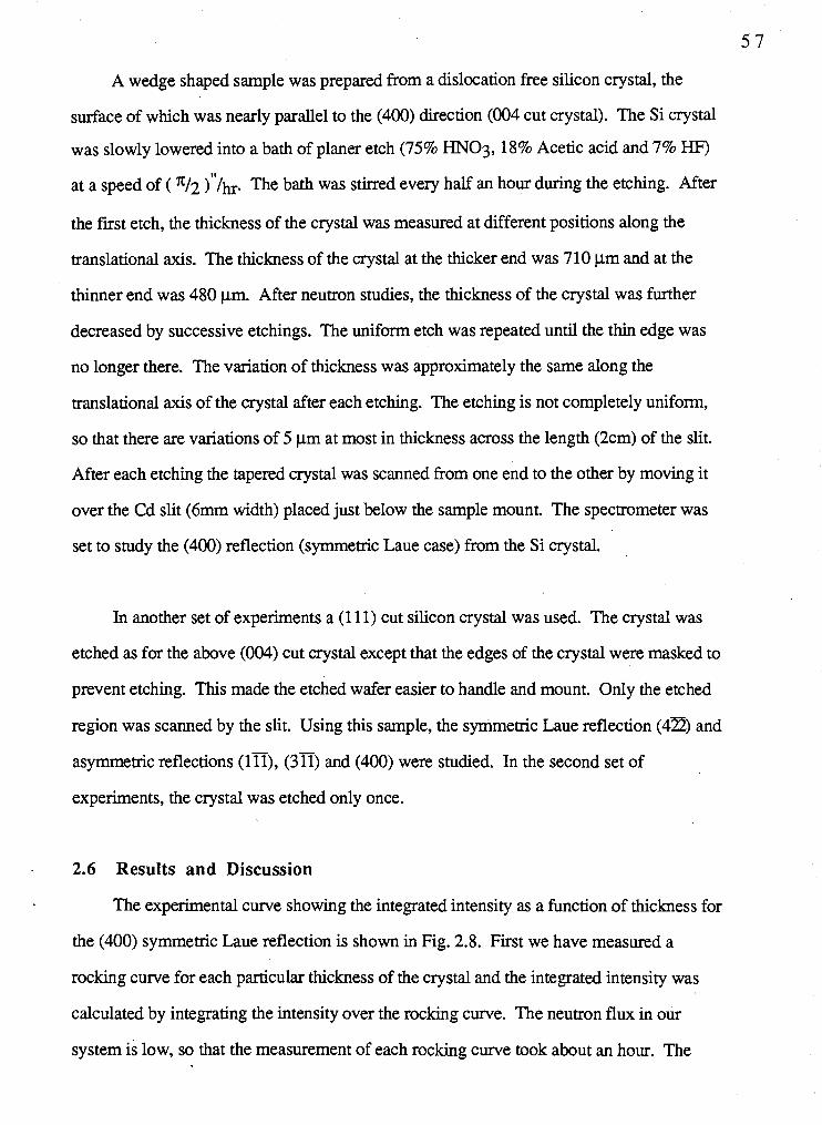
Integrated intensity measured experimentally as a function of thickness

of the crystal for (400) symmetric Laue reflection 5 8

The cross-sectional area of incident and diffracted beams 61

The integrated intensity as a function of position at the exit

surface of the crystal 63

Experimental and theoretical curves of thickness oscillation for (400)

xii

symmetric Laue transmission geometry 65

A schematic representation of the extreme asymmetric Laue case in

which the incident beam is almost parallel to the crystal surface - 68

Dispersion surfaces in the extreme asymmetric Laue case in which

the incident beam is almost parallel to the crystal surface 74

Representation of total external reflection explaining the approximate

and the accurate conditions 75

Misset angle corresponding to the border of the critical region

calculated using the approximate and accurate conditions 77

Intensities of the Bragg diffracted and specular reflected waves as a

function of misset angle in the extreme Laue case 79

The deviation from the Bragg law and EWHM of the envelope of the

diffraction pattern calculated using extended theory, Rustichelli's

formulation and conventional theory 82

Dispersion surfaces in the extreme asymmetric Laue case in which

the Bragg diffracted beam is almost parallel to the crystal surface - 84

Situation explaining the formation of evanescent surface

diffracted waves 85

Misset angles corresponding to the borders of the different regions

in the dispersion surface in the extreme Laue case 87

Intensities of the Bragg diffracted and specular diffracted waves as a

function of misset angle in the extreme Laue case 89

Dispersion surfaces in the extreme asymmetric Bragg case in which

the Bragg diffracted beam is almost parallel to the crystal surface - 9 1

Misset angles corresponding to the borders of the different regions

in the dispersion surface calculated using the approximate and

accurate conditions 93

. . . X l l l

Intensities of the Bragg diffracted and specular diffracted waves as a

function of misset angle in the extreme Bragg case 94

Dispersion surfaces in the extreme asymmetric Bragg case in which

the incident beam is almost parallel to the crystal surface 96

Misset angles corresponding to the borders of the different regions

in the dispersion surface in the extreme Bragg case 99

Intensities of the Bragg diffracted and specular reflected waves as a

function of misset angle in the extreme Bragg case 101

The deviation from the Bragg law and the width of the Darwin

plateau calculated using extended theory, Rustichelli's

formulation and conventional theory 103

Representation of the Borrmann triangle 11 1

The geometry of the crystal experiencing homogeneous bending

which was elaborated by Penning and Polder 116

The mid-surface displacement of a homogeneously bent crystal

elaborated by Penning and Polder 118

Bent crystal rocking curves 121

Integrated intensity as a function of curvature of the bending 123

Integrated intensity as a function of thickness of the crystal for

different values of radius of curvature 124

Scheme of the bending system & the coordinate system of the

bent crystal 126

The mid-surface displacement of a bent crystal in our experimental

set up without and with strain in the z direction 131

CHAPTER 1

INTRODUCTION

1.1 History

Since the advent of nuclear reactors, the neutron has been extensively used to study

condensed matter in general and crystals structures in particular. Thermalized neutrons

from reactors have wavelengths comparable to atomic spacings in crystals. Neutron

diffraction from crystals supplements x-ray diffraction, particularly in distinguishing

among elements on the basis of nuclear cross-sections, which vary strongly from element

to element. For example the neutron is strongly scattered by hydrogen. The mass of the

neutron is well suited to the study of inelastic scattering, for example from phonons in

solids. Because the neutron has a magnetic moment, but no charge, it makes an ideal probe

of the magnetic induction on the atomic scale.

The theory of neutron diffraction, like that of x-ray diffraction is well developed in

the kinematic and dynamic limits. In the kinematic limit small volbmes of matter diffract

intensity from beam to beam. In the dynamical theory one adds the amplitudes of the

waves scattered from atoms. Dynamical theory is applied to small regions of mosaic

crystals to determine the diffracted beam intensities used in the kinematic theory where the

lack of correlation from region to region leads to the addition of intensities. Dynamical

theory must be used to treat the whole problem of diffraction in crystals with a high degree

of correlation over extended volumes. In the study of most crystals it is sufficient to

employ kinematic theory, but with the development of commercially available dislocation

free silicon wafers (up to 20 cm in diameter and 0.5 -1 mm in thickness) it becomes

important to be able to use dynamical theory for large highly correlated crystals. These Si

wafers are an order of magnitude too thick for their optimum employment as neutron

monoc'hromating crystals. By introducing elastic strain gradients into them it is possible to

increase their ability to reflect neutron beams by an order of magnitude. The main purpose

of this study is to increase our understanding of the propagation of neutrons in such

crystals. To accomplish this we start with the dynamic theory of perfect crystals. The next

step is to calculate diffraction from crystals with uniform elastic strain gradients. The final

step is to determine the actual elastic strains in deformed crystals and to apply the dynamical

theory with uniform strain gradients to each small region of the crystal with spatially

varying strain gradients. The elasticity theory of bent crystals is more complicated than one

would gather from most texts on the subject. Rather than one fourth order linear

differential equation one is faced with a pair of coupled non linear fourth order differential

equations.

The dynamical theory of diffraction is highly developed for the x-ray case, beginning

with the historic work of C. G. Darwin, P. P. Ewald and M. V. Laue. The dynamical

theory of x-rays is summarized in the books of Zachariasen [I] and James [2] and more

recent aspects are included in [3]. Since the first observation of Pendellosung fiinge

structure in a neutron diffraction experiment, using perfect single crystals of silicon, by C.

G. Shull in 1968 141, interest in the application of the dynamical theory to the neutron case

has grown substantially. Excellent reviews exist for the neutron case, such as those of

Sears [5] and by Rauch and Petrascheck [6]. The dynamical theory of neutron diffraction

is closely related to the corresponding theory for x-ray diffraction. The main difference is

that, for neutrons, the coherent wave is weakly absorbed in most materials, whereas, for x-

rays, it is very strongly absorbed. This is particularly true for the case of Si crystals.

Dynamical theory provides a theoretical frame work for a number of phenomena which are

absent in the kinematical theory.

1.2 General review of the dynamical theory for a perfect crystal slab + Consider an incoming plane wave of wave vector ko impinging on a slab of perfect

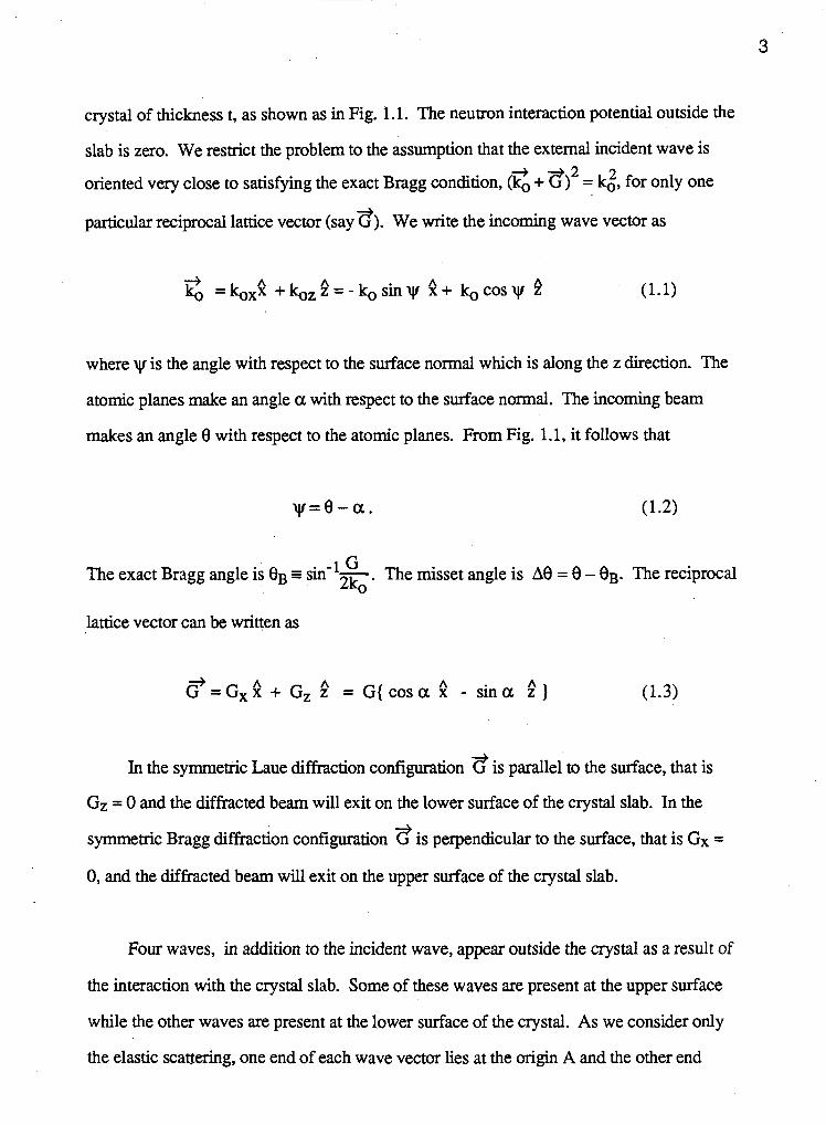
crystal of thickness t, as shown as in Fig. 1.1. The neutron interaction potential outside the

slab is zero. We restrict the problem to the assumption that the external incident wave is + 2

oriented very close to satisfying the exact Bragg condition, (k, + 8) = g, for only one

particular reciprocal lattice vector (say 3). We write the incoming wave vector as

where y~ is the angle with respect to the surface normal which is along the z direction. The

atomic planes make an angle a with respect to the surface normal. The incoming beam

makes an angle 8 with respect to the atomic planes. From Fig. 1.1, it follows that

The exact Bragg angle is eB = sin' - . The misset angle is ~8 = 8 - eB. The reciprocal 2ko

lattice vector can be written as

+ G =G,? + Gz z" = G{cosa ? - s ina 4 ) (1.3)

In the symmetric Laue diffraction configuration -d is parallel to the surface, that is

GZ = 0 and the diffracted beam will exit on the lower surface of the crystal slab. In the

symmetric Bragg diffraction configuration -d is perpendicular to the surface, that is Gx =

0, and the difhcted beam will exit on the upper surface of the crystal slab.

Four waves, in addition to the incident wave, appear outside the crystal as a result of

the interaction with the crystal slab. Some of these waves are present at the upper surface

while the other waves are present at the lower surface of the crystal. As we consider only

the elastic scattering, one end of each wave vector lies at the origin A and the other end

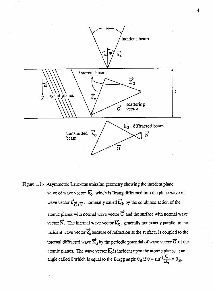
Figure 1.1:- Asymmetric Laue-transmission geometry showing the incident plane -+

wave of wave vector ko , which is Bragg diffracted into the plane wave of +

wave vector k$+$ , nominally called G, by the combined action of the

A internal beams

atomic planes with normal wave vector d and the surface with normal wave

t

v

vector 3. The internal wave vector , generally not exactly parallel to the -+

incident wave vector ko because of refraction at the surface, is coupled to the

internal diffracted wave by the periodic potential of wave vector 5 of the -+

atomic planes. The wave vector his incident upon the atomic planes at an 1 G angle called 8 which is equal to the Bragg angle BB if 8 = sin- - 2k0 - = 'B.

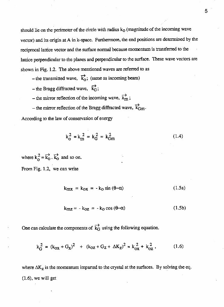
should lie on the perimeter of the circle with radius k~ (magnitude of the incoming wave

vector) and its origin at A in k-space. Furthermore, the end positions are determined by the

reciprocal lattice vector and the surface normal because momentum is transferred to the

lattice perpendicular to the planes and perpendicular to the surface. These wave vectors are

shown in Fig. 1.2. The above mentioned waves are referred to as + - the transmitted wave, ko; (same as incoming beam)

+ - the Bragg diffracted wave, kG ;

+ - the mirror reflection of the incoming wave, km ; + - the mirror reflection of the Bragg diffracted wave, kGm.

According to the law of conservation of energy

where k i = g . and so on.

From Fig. 1.2, we can write

kmx = kox = - ko sin (&a)

+ One can calculate the components of kG using the following equation.

where AK, is the momentum imparted to the crystal at the surfaces. By solving the eq.

(1.6), we will get

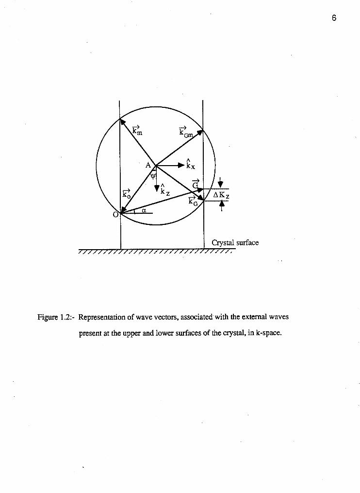
Figure 1.2:- Representation of wave vectors, associated with the external waves

present at the upper and lower surfaces of the crystal, in k-space.

and then

kGx = kG* = (kox + Gx)

(Note:- For the Bragg geometry the signs of kGZ and hmz will interchange.)

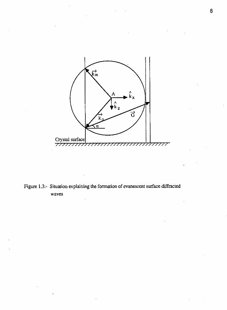
In some cases, as shown as in Fig. 1.3, kcZ and bmz become purely imaginary,

i.e. when the diffracted beam is almost parallel to the crystal surface, for some directions of

incident wave (very close to the exact Bragg condition), the Bragg diffracted wave and the

mirror reflection of the Bragg diffracted wave become evanescent. The condition for this

situation is

Under this condition, both of these evanescent waves are propagated along the

surface of the crystal. The amplitudes of the waves, which are propagated along the lower

and upper surfaces of the crystal, are damped in the (-ve) and (+ve) z direction respectively

in order that the amplitude = 0 at +oo. The calculations are shown in chapter 3.

The amplitudes of the specified external waves are found by matching the waves

internal and external to the slab. The external wave vectors select among the many

possible internal wave vectors. In particular the components parallel to the surface of the

internal wave vectors must match the components parallel to the surface of the external

Crystal surfact /////////

Figure 1.3:- Situation explaining the formation of evanescent surface diffracted waves

wave vectors. The possible internal wave vectors are determined by solving Schriidinger's

equation for the neutron, which contains the periodic neutron-nuclear interaction potential

inside the crystal. This determines the relations between the components of the internal

wave vectors and the other known quantities such as magnitude of the incident wave vector

and the fourier components of the periodic interaction potential. These are called the

dispersion relations. A given kox of the incoming wave will select four internal waves

A3'C'D = bx and four coherently generated Bragg rt,", rt,B, 2: and 2: all with G~ A +B +C diffracted waves 6 , KG , KG and SD all with K&'B'CP = kox + Gx. As $ =

ft, + $, the dispersion relations determine the four values of G, that go with both Kox

and KG,. We now justify these remarks in more detail.

, The time independent Schrijdinger equation for a neutron inside a crystal is

h2 + - - 2m v2y ( t ) + v(;)Y(;~) = E~ ~ ( r ) , (1.10)

where V (7) is the interaction potential of the neutron inside the crystal, and Eo is the

incident neutron kinetic energy,

The total energy of the neutron inside the crystal is Eo. For the perfect crystal V (7) is periodic. If we define a reduced potential with the dimensions of ko2,

we can write eq. (1.10) as

The reduced periodic neutron-nuclear interaction potential for a rigid array of nuclei can be

written as

where the position vector of the lth nucleus is denoted by Rl and bl is the scattering length

of that nucleus, or can be expanded in a Fourier series

By Fourier analyzing the above expression we will get

++ where F+ = x bl di 'R1 is the unit cell structure factor and V c e ~ is the volume of a

G 1

unit cell.

4 Using the assumption that the incident wave vector ko is oriented very close to the

exact Bragg condition for the particular reciprocal lattice vectorz, only the Fourier

components of the potential associated with 8, normal to the reflecting planes, become

important. Thus, we write

where vo is the average potential inside the crystal with respect to the potential outside the

crystal which is zero, i.e. the potential which corresponds to zero reciprocal lattice vector.

Note that for the silicon crystals I v(22O) I = a 1 v(ll1) I = vo e-W, where w is the Debye-

Waller temperature factor. Furthermore, for a non absorbing, centrosymrnetric crystal v--+ G

= v . The typical values of vo and v+ for silicon crystals are given in appendix 1. As -G G

the periodic potential couples the incident wave with the diffracted wave, the neutron wave

function can be expanded in Bloch functions

ti

Under the same assumption as above, only two amplitudes Yo and YG, will be large.

Thus we anticipate the solutions of eq. (1.13) to be of the form

where

By substituting this wave function into the Schriidinger equation (1.13) together with

(1.15) and comparing the coefficients of the fourier components on both sides, we get a

pair of linear algebraic equations:

2 2 + (ko-vO-&)yG = 0. (1.18b)

For a non trivial solution of eqs. (1.18) to exist, the determinant of the coefficients of Yo

and YG must vanish, i.e.

This is known as a "dispersion relation". (Note that from here onwards we will drop the vector sign appearing in v+ and v +.)

G -G

The neutron wave function must be continuous at the boundary and so the

components parallel to the surface of the internal and external wave vectors must match.

Therefore we can write the following relations for the parallel sided slab:

and

We see that the dispersion relation (eq. (1.19)) becomes quartic in KO, by substituting the + + eqs. (1.20). One can now see that, a given incident plane wave <po exp ( k, . r ) generates

A,B,CP - four internal waves having wave vectors sA, 3:. 3: and SD with KOx -

bx. These four waves in turn generate, and are coherently coupled to, four Bragg A +B A,B,C,D diffracted internal waves having wave vectors 6 , Kg , and with Gx

= kox + Gx. Consequently the total wave in'side the crystal consists of coherent

superposition of eight plane waves, i.e.

2 To the extent that VGVG cc &, and v ~ v ~ cc k2 (i.e. VGV.G = O), the quartic

relation describes two intersecting spheres, one centered at the origin 0 and the other at G,

both of radius .I=. These spheres are the asymptotic forms of the dispersion

surface; We treat the case where the incident wave vector, the reciprocal lattice vector and

the surface normal all lie in the same plane which cuts the spheres into two circles. The

equation of the asymptotic circles is given by

The solutions selected by the boundary conditions are found by intersecting the dispersion

surface with a line which is normal to the crystal surface at the value of kx. This line

intersects the asymptotic circles at four points with coordinates

and

2 where A = Gx + 2 bx Gx, hz = cos (8 - a), kox =- k, sin (8 - a), Gz = - G sin a,

and Gx = G cos a. The fmt two roots are for the circle of ( g - vo - K:) = 0 and the last

two roots are for the circle of (g - vo - g) = 0. By knowing these roots, we can rewrite

the dispersion relation in the form

A A C P with Kox = kox. The solutions of the above eq. (1.23) give the exact values of

&,. The term v ~ v - G leads to a splitting of the two circles into an outside curve (a -

branch) and an inside curve (P - branch) as shown in Fig. 1.4.

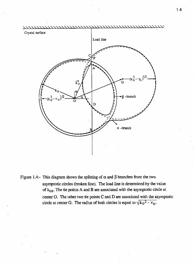
Figure 1.4:- This diagram shows the splitting of a and P branches from the two

asymptotic circles (broken line). The load line is determined by the value of 16,. The tie points A and B are associated with the asymptotic circle at

center 0. The other two tie points C and D are associated with the asymptotic circle at center G. The radius of both circles is equal to d G

The boundary conditions for the parallel-sided slab then lead to the values for the

corresponding eight internal wave amplitudes and four unknown external wave amplitudes

in terms of the known incident wave amplitude ao. The boundary conditions at the crystal

surfaces are

- the continuity of the waves,

- the continuity of the gradients of the waves normal to the surface.

If quartic equations were sufficiently transparent, one would just write down the

expressions for the eight waves and let it go at that. These things are handled readily by

computers using complex arithmetic. To obtain useful analytic expressions some

approximations are called for. These approximations, corresponding to different

situations, are explained later in this chapter. This approach of solving the parallel-sided

slab problem is known as the "eikonal approach".

There is an alternative mathematical approach to solve the parallel-sided slab problem.

In this approach, we again solve the Schrijdinger's equation (1.13), but now the

amplitudes yo(?) and yG(?) of the waves inside the crystal are allowed to depend upon

+ position. Under the assumption that the incident wave vector k, is oriented very close to

the exact Bragg condition for a particular reciprocal lattice vector, we again anticipate the

solution inside the crystal of the form

whereagain $ = + d .

-+ In particular, we will choose the internal wave vector K, to satisfy the exact Bragg

condition for one particular scattering wave vector 8 and to have magnitude

Note that the external Bragg angle eB is given by

whereas the internal Bragg angle (i$ is given by

A A We set up an oblique coordinate system choosing unit vectors soalong ?o and SG

along as shown in Fig. 1.5. The relations between the oblique coordinate system

(So,SG) and the rectangular axes chosen to be parallel (x) and perpendicular (z) to the

surface of the slab (see Fig. 1.5) are:

I so = ( z s i n ( ~ ~ + a ) - x c o s ( ~ ; + a ) ~

sin 20;

and

SG = {z sin (8; - a ) + x cos (8; - a ) } . sin 28;

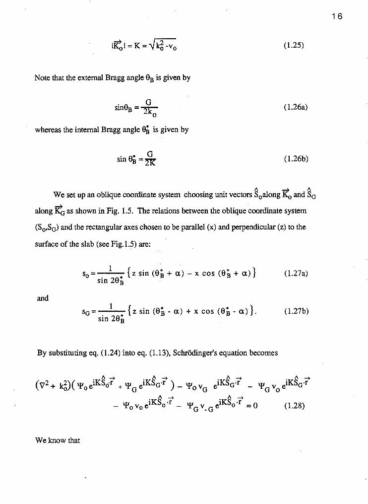
By substituting eq. (1.24) into eq. (1.13), Schriidinger's equation becomes

We know that

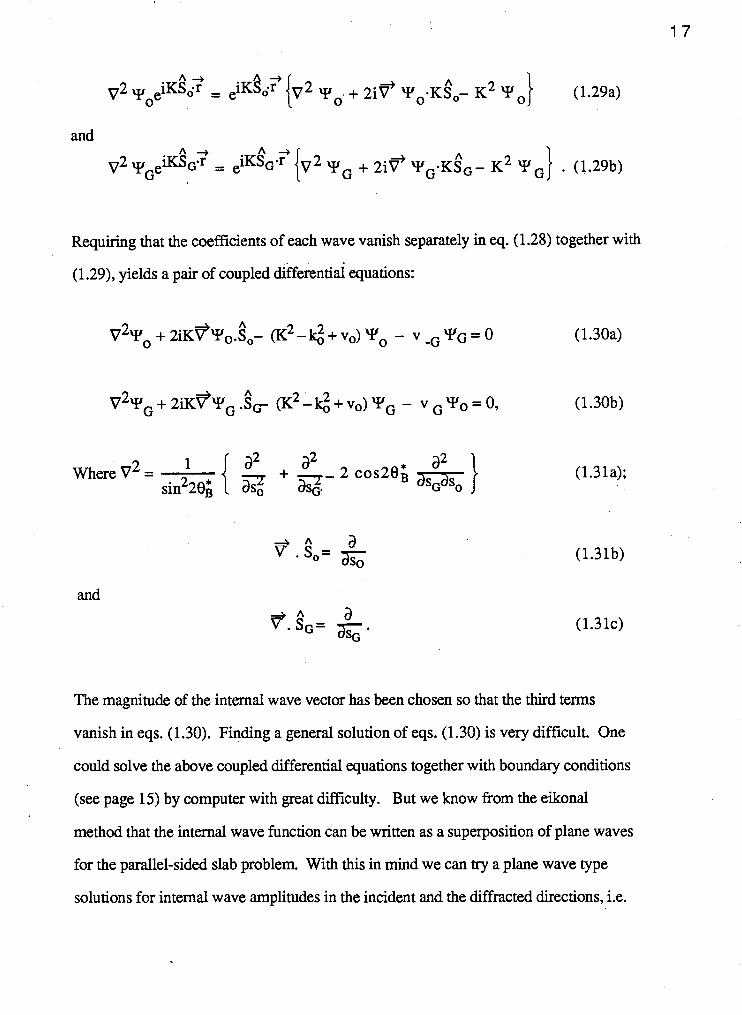
and A + A v2 Y ~ ~ ~ ~ ~ G ' ~ = + 2iP) YG.KSG - K2 Y . (1.29b)

Requiring that the coefficients of each wave vanish separately in eq. (1.28) together with

(1 .B), yields a pair of coupled differential equations:

and

The magnitude of the internal wave vector has been chosen so that the third terms

vanish in eqs. (1.30). Finding a general solution of eqs. (1.30) is very difficult. One

could solve the above coupled differential equations together with boundary conditions

(see page 15) by computer with great difficulty. But we know from the eikonal

method that the internal wave function can be written as a superposition of plane waves

for the parallel-sided slab problem. With this in mind we can try a plane wave type

solutions for internal wave amplitudes in the incident and the diffracted directions, i.e.

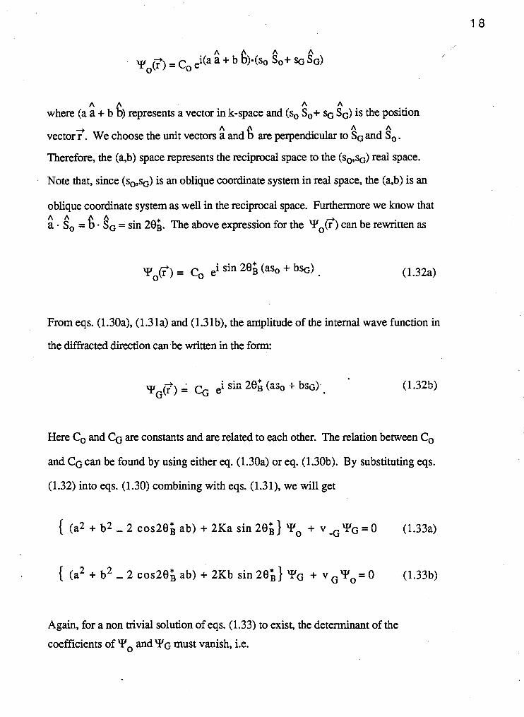
A A A A where (a a + b b) represents a vector in k-space and (so So+ sc SG) is the position

A 6 A A vector?. We choose the unit vectors a and are perpendicular to So and So.

Therefore, the (ii,b) space represents the reciprocal space to the (so,sG) real space.

Note that, since (sO,sG) is an oblique coordinate system in real space, the (a,b) is an

oblique coordinate system as well in the reciprocal space. Furthermore we know that A A A a . So = 6. SG = sin 28;. The above expression for the yo(?) can be rewritten as

Y~(?) = Co e i sin 28; (aso + bsG)

From eqs. (1.30a), (1.3 la) and (1.3 lb), the amplitude of the internal wave function in

the diffracted direction can be written in the form:

. . = CG e i sn 28; (as, + bsc).

Here Co are constants and are related to each other. The relation between Co

and CG can be found by using either eq. (1.30a) or eq. (1.30b). By substituting eqs.

(1.32) into eqs. (1.30) combining with eqs. (1.31), we will get

{ (a2 + b2 - 2 cos28; ab) + 2Ka sin 28;) Yo + v -GYG = 0 (1.33a)

{ (a2 + b 2 - 2 cos28;ab) + 2 ~ b sin20;) yG + v G Y 0 = 0 (1.33b)

Again, for a non trivial solution of eqs. (1.33) to exist, the determinant of the

coefficients of Yo and YG must vanish, i.e.

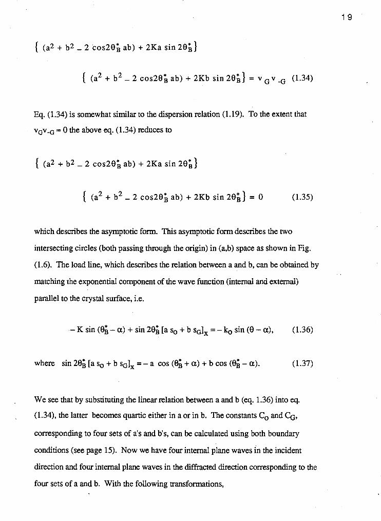
{ (a2 + b2 - 2 cos29; ab) + 2Ka sin 29;)

{ (a2 + b2 - 2 cos29; ab) + 2Kb sin 29;) = v G~ -G (1.34)

Eq. (1.34) is somewhat similar to the dispersion relation (1.19). To the extent that

VGV-G = 0 the above eq. (1.34) reduces to

{ (a2 + b2 - 2 cos29; ab) + 2Ka sin 29;)

{ (a2 + b2 - 2 cos28; ab) + 2Kb sin 29;) = 0 (1.35)

which describes the asymptotic form. This asymptotic form describes the two

intersecting circles (both passing through the origin) in (a,b) space as shown in Fig.

(1.6). The load line, which describes the relation between a and b, can be obtained by

matching the exponential component of the wave function (internal a d externalj

parallel to the crystal surface, i.e.

where sin 2% [a so + b so], = - a cos (6 + a) + b cos ($ - a). (1.37)

We see that by substituting the linear relation between a and b (eq. 1.36) into eq.

(1.34), the latter becomes quartic either in a or in b. The constants Co and CG,

corresponding to four sets of a's and b's, can be calculated using both boundary

conditions (see page 15). Now we have four internal plane waves in the incident

direction and four internal plane waves in the diffracted direction corresponding to the

four sets of a and b. With the following transformations,

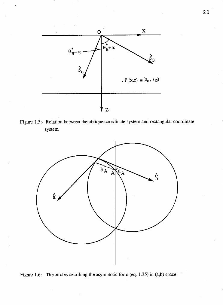
Figure .5:- Relation between the oblique coordinate system and rectangular

system

coordinate

Figure 1.6:- The circles decribing the asymptotic form (eq. 1.35) in (a,b) space

{(Kx,K,) are components of the internal wave vector in the eikonal approach.), we

could recover all the eight internal waves which we got in the eikonal approach. Thus

we would get nothing new. However, the advantage of this method in certain

geometries and also in treating the strain problem (under some assumptions suitable for

these situations) are briefly discussed later in this chapter. I will call this second

approach the "spatially dependent amplitude method" in rest of my thesis.

1.3 The scope of this thesis

When treating the strain gradient problem we will look for approximate solutions of

Schriidinger's equation. The approximations in the eikonal method and in the spatially

dependent amplitude method are conceptually different. We will show for the unstrained

crystal slab that they lead to almost the same results in most cases. In order to understand

some of the differences, we will study some extreme cases in which either the incoming or

outgoing beam is very close to paralleling the surface. When we treat the elastic strain

gmhent problem we will do it using the spatially dependent amplitude method But we

will already have some understanding of the effects that cannot be obtained from this

method in the unstrained crystal. The approximate treatment using the spatially dependent

amplitude method is commonly referred to as the T-T method in the literature in recognition

of the contributions of Takagi and Taupin.

To discuss what comes into the T-T method applied to crystals with strain gradients it

is first necessary to discuss the T-T method applied to the unstrained crystal. After this we

will return to outline what is involved in the study of diffraction from crystals with strain

gradients and also to discuss the strain itself and Row it is determined using elasticity

theories for single crystals in the form of thin plates.

1.3.1 Approximations in the eikonal approach

In the eikonal approach, only four internal waves out of eight internal waves become

important in most cases except extreme asymmetric cases. In other words the amplitudes

of the other four internal waves are negligible. In the literature, researchers in this field use

different approximations in order to reduce the eight wave problem into a four wave

problem. Sometimes these approximations confuse the reader. Therefore we will state the

approximations very clearly.

For example we will consider the non extreme asymmetric Laue geometry and will

state all the approximations. The dispersion surfaces, which determine the internal wave

vectors, for this particular case are shown in Fig. 1.4 @age 14). The tie points A and C are

closer to one end (P) of the incident wave vector. The four internal waves with wave

vectors sA, 22, R!: and e, corresponding to these two tie points (A and C) are A C

important here. Note that the two z components &-,, and &-,, are close to each other and

to the value of hz (z component of the incident wave vector). Therefore these two z

components have to be calculated more accurately using the dispersion relation (1.23). We

can rewrite the dispersion relation (1.23) in the form

We can approximate the above equation (1.39) to

*A *C in this particular case. This has been done by replacing I?,, by KO, and hz in the right

*A hand side of the equation (1.39) which is small. Note that the asymptotic roots and *B *C Koz correspond to the asymptotic circle with center at 0 while the other two roots Koz

*D and KO, correspond to the asymptotic circle which center is at G. Thus, the right hand

side of the eq. (1.40) will take the simplest form. The quantity E is an energy in reduced

2 units of (inverse length) . It sets the length scale for pendellosung effects in dynamical

theory, as will be seen in chapter 2. By solving the above quadratic equation (1.40), we A C can calculate accurate values for KO, and KO,. Since the tie points B and D are far away

*B *D B D from point P, we can use the asymptotic values and I?,= for I?,, and I?,z.

By using the two boundary conditions mentioned earlier, one could calculate all eight

internal wave amplitudes and four unknown external wave amplitudes. This can be done

numerically very easily, but we see that the amplitudes of the four internal waves

cmesponchg to ~ l e tie B and D are negligible. We take them to be zero.

Furthermore, the amplitudes of two external waves (mirror reflection of the incoming wave

and of Bragg diffracted wave) are negligible in this case. For simplicity we take them to be

zero as well. Now we have only four internal waves and three external waves including

the incoming wave. By using the boundary condition, continuity of internal and external

waves at the crystal surfaces, we can find analytical expressions for the amplitudes of the

four internal waves and of the two unknown external waves in terms of the known

incoming wave amplitude aO' Since we have omitted four internal waves and two external

waves, it is unnecessary to invoke the second boundary condition, continuity of the

gradients of the waves normal to surface. Similar approximations are applicable to the non

extreme asymmetric Bragg geometry. Calculations in these cases are made and analytical

expressions are given in chapter 2.

1.3.2 The T-T method

In these non extreme cases, we can reduce the spatially dependent amplitude method

to the T-T method. Here, we take advantage of the fact that the amplitudes of the wave

function (eq. 1.24) inside the crystal are slowly varying (much slower than that of the 2 carrier wave), so that terms involving V Yo which are numerically small compared to

A KSo .vy0 , are neglected. This assumption has an effect similar to the omission of four

internal waves in the eikonal approach. Now using the oblique coordinates, one obtains a

simple form to the coupled differential equations (1.30a & b):

and

which combine to give a second order partial differentialequation for YG:

We can solve the equations (1.41) together with the boundary condition, continuity of

waves at the crystal surfaces, and determine the amplitudes of the internal and external

waves. By rearranging the complete internal wave function, we will get four plane

waves which seem similar to those obtained in the eikonal approach. But the results

obtained by these two methods are not quite same because the approximations are different.

These remarks are justified in more detail in chapter 2.

The T-T method has a unique advantage. For certain geometries, the solutions of the

equations (1.41) are straight forward. For a "6 - function" incident beam (narrow slit

geometry), the solutions are in the form of Bessel functions [7]. This spatially dependent

amplitude method with the above mentioned assumption was first developed by Takagi [8]

and Taupin [9] to study the effects of strain in the dynamical diffraction of x-rays and more

recently utilized by Werner [lo] to calculate the effects of gravitational and magnetic fields

on the diffraction of neutrons.

We have calculated the integrated diffracted beam intensity (at the exit surface) as a

function of crystal thickness for non extreme asymmetric Laue cases. In order to verify

these results, experiments were performed in the symmetric and non extreme asymmetric

Laue geometry. In these experiments, we have measured the dependence of the diffracted

beam intensity as a function of thickness of Si wafers successively etched to thinner and

thinner dimensions. The comparison of theory and experiments are given in chapter 2.

1.3.3 The extreme cases

The above described four wave theory (conventional theory) starts to fail in extreme

asymmetric cases. These extreme cases can be divided into four categories. They are

1. incident beam almost parallel to the crystal surface (Laue geometry)

2. Bragg diffracted beam almost parallel to the crystal surface (Laue geometry)

3. Bragg diffracted beam almost parallel to the crystal surface (Bragg geometry)

4. incident beam almost parallel to the crystal surface (Bragg geometry).

Theoretically, these cases are obtained by rotating the incident beam and the reciprocal

lattice vector with respect to the crystal surface. In experiments, one can obtain these cases

by cutting the crystal surface at different angles with respect to the reciprocal lattice vector

and by choosing the proper incident beam where the incident beam is oriented very close to

satisfying the exact Bragg condition for that particular reciprocal lattice vector.

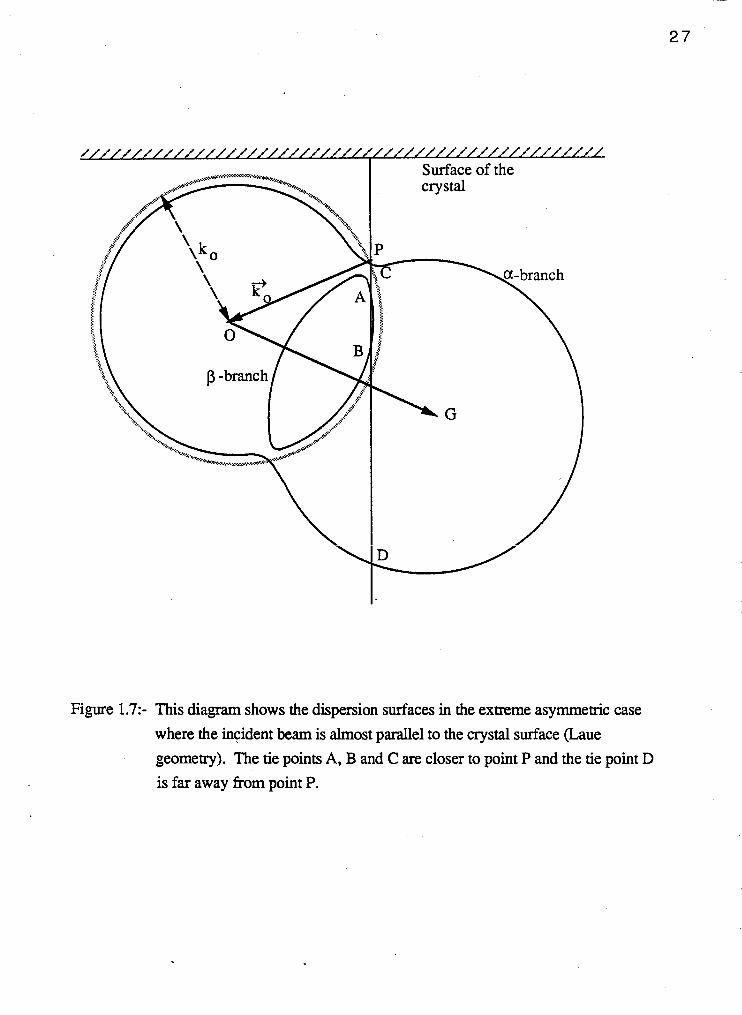
In the extreme asymmetric cases, more than four waves become important. We

consider the case where the incident beam is almost parallel to the crystal surface as an

example. The dispersion surface which gives the internal wave vectors are shown in Fig.

1.7 for this particular case. As we see from the Fig. 1.7, the tie points A, B and C are

close to each other and to point P. Therefore, six waves corresponding to these tie points A B C

A, B and C are important in this case. The three z components ( Gz , Gz and G z ) can

be dete-ed accurately using the dispersion relation in the form

We can approximate the above equation to

which is a cubic equation with coefficients as shown:

Since the tie point D is far away from point P (see Fig. 1.7), we have used the asymptotic *D D

value GZ for KOz .

Furthermore the amplitude of the mirror reflection of the incident wave becomes

significant. In this case we see that at least six internal waves and four external waves,

including the incident wave, are important (i.e. the amplitudes of these waves have

significant values.). The amplitudes of the internal wave associated with the tie point D and

#/1//////1///////////,/

Surface of the crystal

Figure 1.7:- This diagram shows the dispersion surfaces in the extreme asymmetric case where the incident beam is almost parallel to the crystal surface (Laue geometry). The tie points A, B and C are closer to point P and the tie point D is far away from point P.

of the mirror reflection of the Bragg diffracted wave are negligible in this case. For

simplicity we assume them to be zero. To calculate the amplitudes of the important internal

and external waves, we have to use both boundary conditions mentioned earlier. Using

these boundary conditions and ratio of amplitudes (from eqs. (1.18)), we will get a number

of equations which is more than the number of unknowns. One will find easily that two of

these equations become approximately equivalent to two other equations. Therefore,

among the equivalent equations, one of each pair can be omitted in calculating the unknown

internal and external wave amplitudes. Now, we have a number of equations which is

equal to the number of unknowns. The detailed calculations are shown in chapter 3. The

discrepancies among the results obtained using the four wave conventional theory and the

above described modified theory in extreme cases, are discussed in the same chapter. In

addition, the other three extreme cases with detailed calculations are also described. Note

that in all of these four extreme cases, only three tie points are close to the point P. So we

have to calculate at most three values z components of the internal wave vectors more

accurately. Therefore we meed not solve the quartic equation except in the extreme extreme .

case of both incoming and out going wave vectors being close to parallel to the surface.

In the spatially dependent amplitude method, terms like v2yo and v2yG cannot be

neglected in these extreme cases. So we have to solve the coupled differential equations

(1.30) together with boundary conditions. First we have to calculate four sets of values for

a and b from the eqs. (1.34), (1.36) and (1.37). Only three sets of a and b which are close

to zero, are important in the extreme cases. One could proceed and solve the problem in the

same way as we did in the eikonal approach. However, here we have two variables a and

b instead of the one variable KO, in the eikonal approach. Furthermore, the asymptotic *

values of a and b are not trivial. But, the asymptotic value of I?,, (KO,) is known.

Therefore the eikonal approach becomes easier than the spatially dependent amplitude

method in solving the extreme cases of parallel-sided slab geometries.

1.3.4 Elastically deformed crystals

We have treated the elastically deformed crystal problem in the case of a uniform

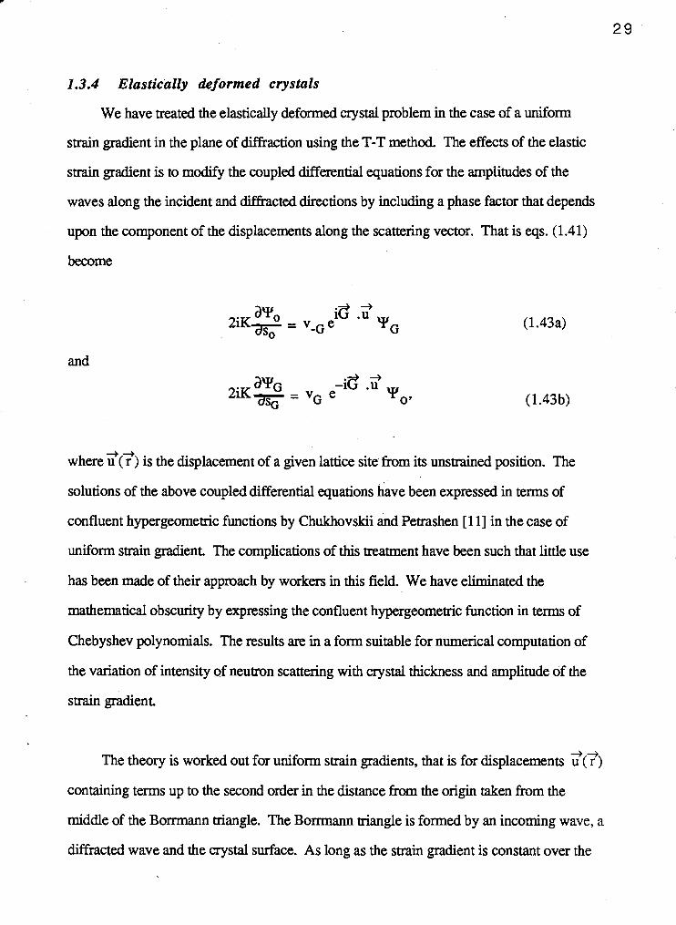
strain gradient in the plane of diffraction using the T-T method. The effects of the elastic

strain gradient is to modify the coupled differential equations for the amplitudes of the

waves along the incident and diffracted directions by including a phase factor that depends

upon the component of the displacements along the scattering vector. That is eqs. (1.41)

become

and

++ where u ( r ) is the displacement of a given lattice site from its unstrained position. The

solutions of the above coupled differential equations have been expressed in terms of

confluent hypergeometric functions by Chukhovskii and Petrashen [l 11 in the case of

uniform strain gradient. The complications of this treatment have been such that little use

has been made of their approach by workers in this field. We have eliminated the

mathematical obscurity by expressing the confluent hypergeometric function in terms of

Chebyshev polynomials. The results are in a form suitable for numerical computation of

the variation of intensity of neutron scattering with crystal thickness and amplitude of the

strain gradient.

++ The theory is worked out for uniform strain gradients, that is for displacements u ( r )

containing terms up to the second order in the distance from the origin taken from the

middle of the Bonmann triangle. The Borrmann triangle is formed by an incoming wave, a

diffracted wave and the crystal surface. As long as the strain gradient is constant over the

Bomnann triangle standard treatment using the T-T method is applicable. The solutions for

uniform strain gradients will apply point by point along the crystal as long as the strain

gradients vary very slowly on the scale of the Bonmann triangle. For example the theory

would apply in the far field of a single dislocation even though it would be quite suspect if

the dislocation was in the middle of the Bornnann mangle.

1.3.5 Elastic strain gradients

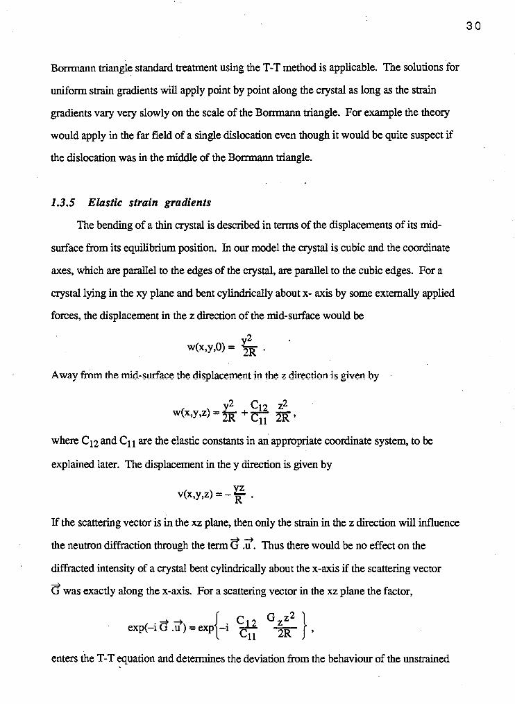
The bending of a thin crystal is described in terms of the displacements of its mid-

surface from its equilibrium position. In our model the crystal is cubic and the coordinate

axes, which are parallel to the edges of the crystal, are parallel to the cubic edges. For a

crystal lying in the xy plane and bent cylindrically about x- axis by some externally applied

forces, the displacement in the z direction of the mid-surface would be

Away from the mid-surface the displacement in the z dkction is given by

where C12 and C1 are the elastic constants in an appropriate coordinate system, to be

explained later. The displacement in the y direction is given by

If the scattering vector is in the xz plane, then only the strain in the z direction will influence

the neutron diffraction through the term d .?. Thus there would be no effect on the

diffracted intensity of a crystal bent cylindrically about the x-axis if the scattering vector

8 was exactly along the x-axis. For a scattering vector in the xz plane the factor,

+ exp(-i 8' .u ) = exp C12 Gzz2

enters the T-T equation and detenrdnes the deviation from the behaviour of the unstrained

crystal.

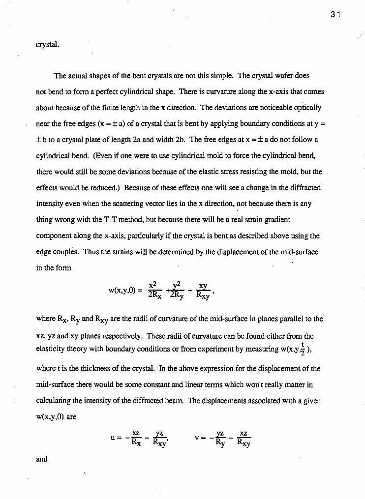
The actual shapes of the bent crystals are not this simple. The crystal wafer does

not bend to foxm a perfect cylindrical shape. There is curvature along the x-axis that comes

about because of the finite length in the x direction. The deviations are noticeable optically

near the free edges (x = f a) of a crystal that is bent by applying boundary conditions at y =

It b to a crystal plate of length 2a and width 2b. The fiee edges at x = + a do not follow a

cylindrical bend. (Even if one were to use cylindrical mold to force the cylindrical bend,

there would still be some deviations because of the elastic stress resisting the mold, but the

effects would be reduced.) Because of these effects one will see a change in the diffracted

intensity even when the scattering vector lies in the x direction, not because there is any

thing wrong with the T-T method, but because there will be a real strain gradient

component along the x-axis, particularly if the crystal is bent as described above using the

edge couples. Thus the strains will be determined by the displacement of the mid-surface

where Rx, Ry and Rxy are the radii of curvature of the mid-surface in planes parallel to the

xz, yz and xy planes respectively. These radii of curvature can be found either from the t elasticity theory with boundary conditions or fiom experiment by measuring w(x,yq ),

where t is the thickness of the crystal. In the above expression for the displacement of the

mid-surface there would be some constant and linear terms which won't really matter in

calculating the intensity of the difhcted beam. The displacements associated with a given

and

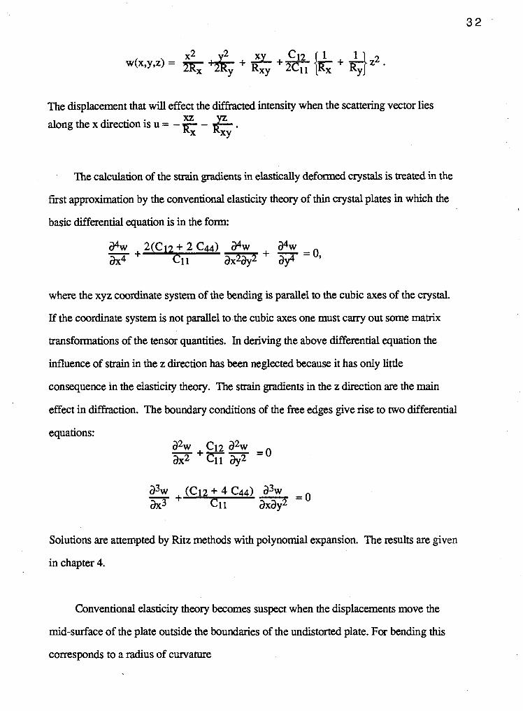
The displacement that will effect the diffracted intensity when the scattering vector lies

along the x direction is u = - - - z, Rx Rxy

The calculation of the strain gradients in elastically deformed crystals is treated in the

first approximation by the conventional elasticity theory of thin crystal plates in which the

basic differential equation is in the form:

where the xyz coordinate system of the bending is parallel to the cubic axes of the crystal.

If the coordinate system is not parallel to the cubic axes one must cany out some matrix

transfoxmations of the tensor quantities. In deriving the above differential equation the

influence of strain in the z direction has been neglected because it has only little

consequence in the elasticity theory. The strain gradients in the z direction are the main

effect in diffraction. The boundary conditions of the free edges give rise to two differential

eauations:

Solutions are attempted by Ritz methods with polynomial expansion. The results are given

in chapter 4.

Conventional elasticity theory becomes suspect when the displacements move the

mid-surface of the plate outside the boundaries of the undistorted plate. For bending this

corresponds to a radius of curvature

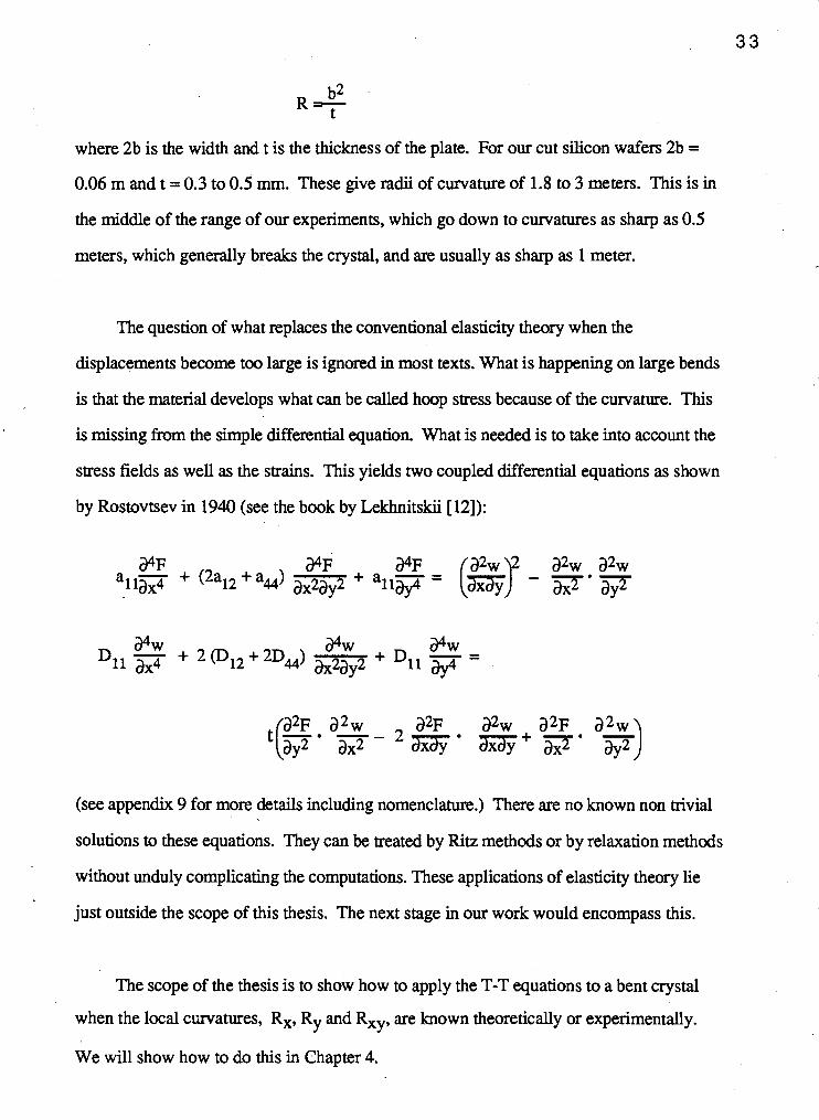
where 2b is the width and t is the thickness of the plate. For our cut silicon wafers 2b =

0.06 m and t = 0.3 to 0.5 mm. These give radii of curvature of 1.8 to 3 meters. This is in

the middle of the range of our experiments, which go down to curvatures as sharp as 0.5

meters, which generally breaks the crystal, and are usually as sharp as 1 meter.

The question of what replaces the conventional elasticity theory when the

displacements become too large is ignored in most texts. What is happening on large bends

is that the material develops what can be called hoop stress because of the curvature. This

is missing from the simple differential equation. What is needed is to take into account the

stress fields as well as the strains. This yields two coupled differential equations as shown

by Rostovtsev in 1940 (see the book by Lekhnitskii [12]):

(see appendix 9 for more details including nomenclature.) There are no known non trivial

solutions to these equations. They can be treated by Ritz methods or by relaxation methods

without unduly complicating the computations. These applications of elasticity theory lie

just outside the scope of this thesis. The next stage in our work would encompass this.

The scope of the thesis is to show how to apply the T-T equations to a bent crystal

when the local curvatures, R , Ry and Rxy, are known theoretically or experimentally.

We will show how to do this in Chapter 4.

CHAPTER 2

CONVENTIONAL DYNAMICAL THEORY OF DIFFRACTION

2.1 The eikonal approach

Here we give detailed calculations of internal wave vectors (important ones only) and

of corresponding internal wave amplitudes in the case of symmetric and non extreme

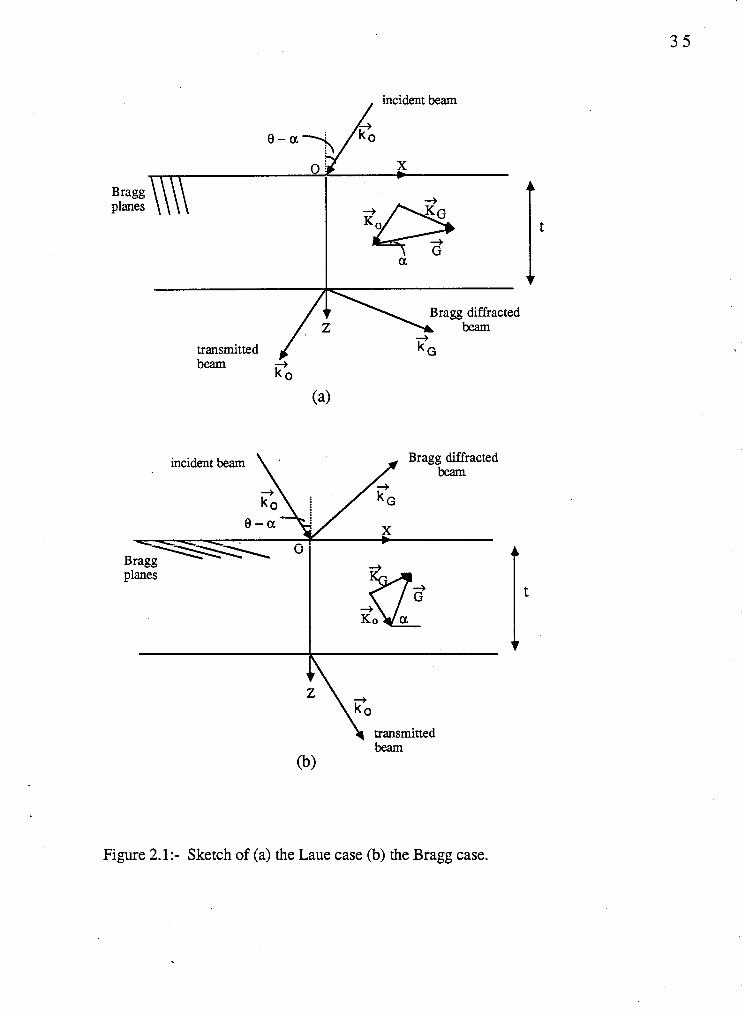
asymmetric Laue and Bragg geometries. We distinguish now between the Laue case (Fig.

2. la) and the Bragg case (Fig. 2.1 b). There are some differences in solving the parallel-

sided slab problem between Laue and Bragg cases. We will state the differences wherever

they occur.

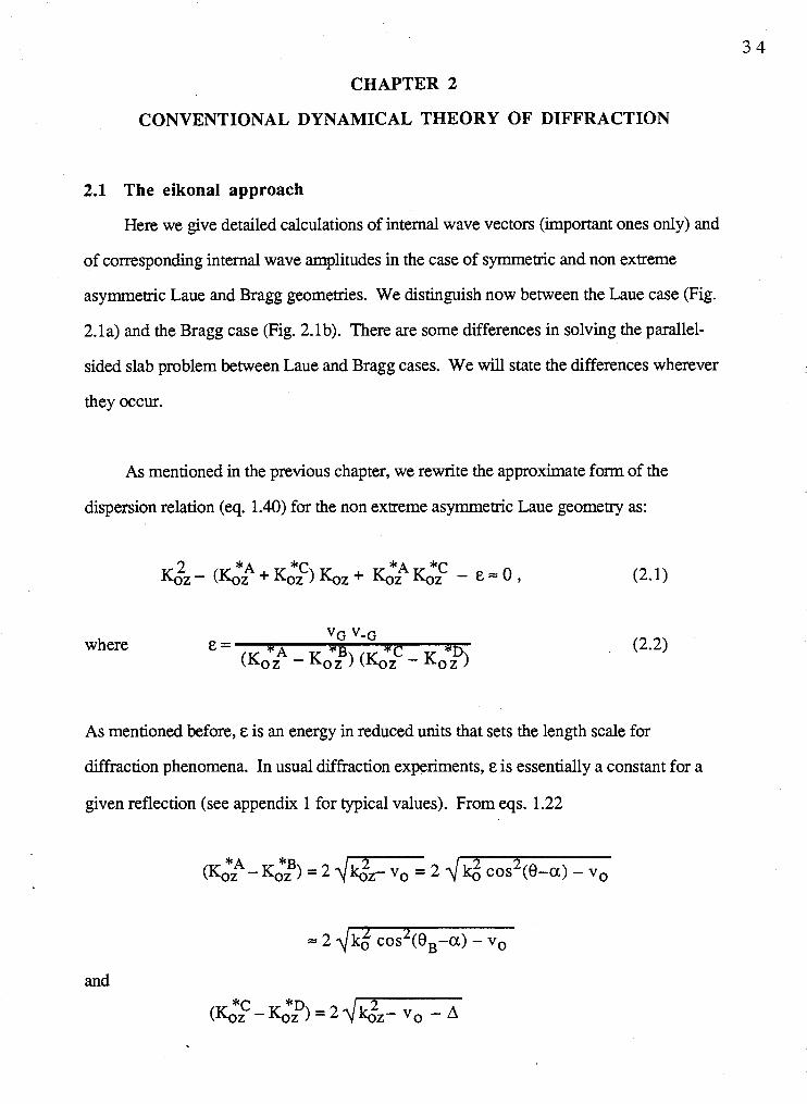
As mentioned in the previous chapter, we rewrite the approximate form of the

dispersion relation (eq. 1.40) for the non extreme asymmetric Laue geometry as:

where

As mentioned before, r is an energy in reduced units that sets the length scale for

diffraction phenomena. In usual diffraction experiments, E is essentially a constant for a

given reflection (see appendix 1 for typical values). From eqs. 1.22

and

B r a s planes

transmitted beam co / Bragg diffracted

+ k,

Bragg diffracted beam

0

planes

\ transmitted beam

(b)

Figure 2.1 :- Sketch of (a) the Laue case (b) the Bragg case.

2 2 2 2 = 2 .\1bcos (0-a) - vo - G cos a + 2koGsin(0-cx)cosa

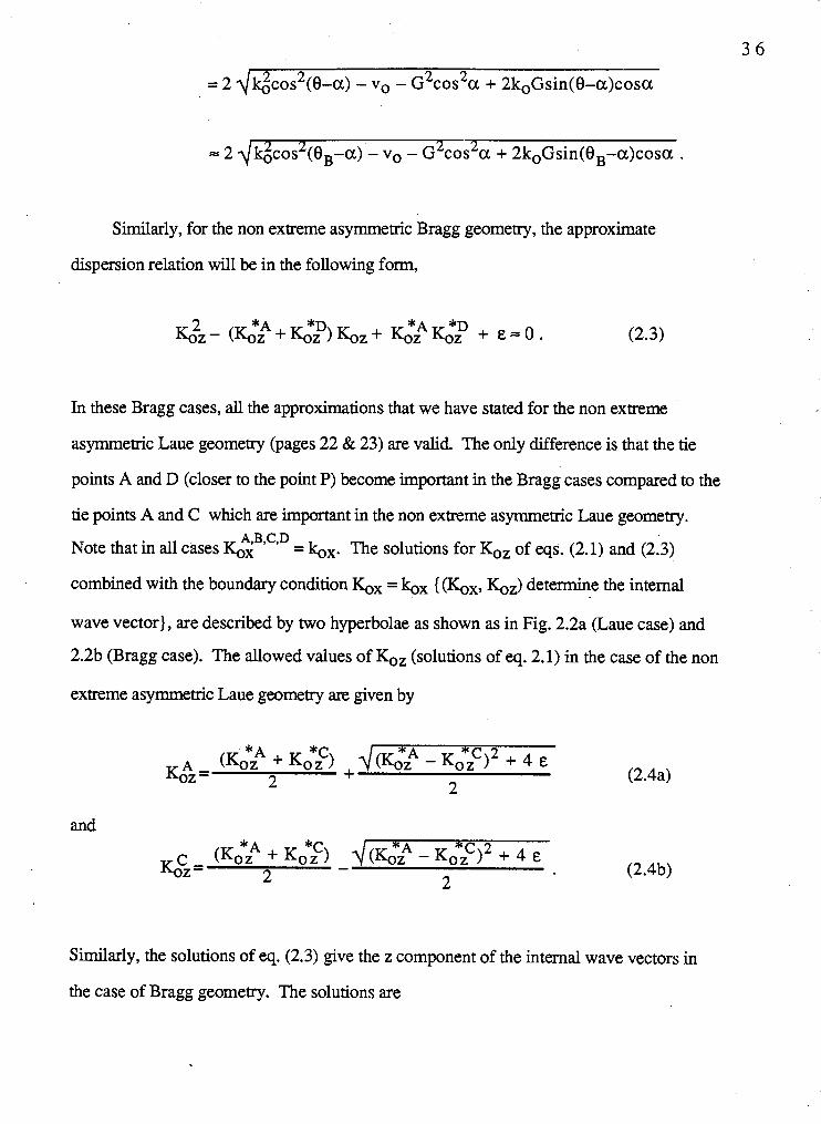
Similarly, for the non extreme asymmetric Bragg geometry, the approximate

dispersion relation will be in the following form,

In these Bragg cases, all the approximations that we have stated for the non extreme

asymmetric Laue geometry (pages 22 & 23) are valid The only difference is that the tie

points A and D (closer to the point P) become important in the Bragg cases compared to the

tie points A and C which are important in the non extreme asymmetric Laue geometry. A,B.C,D Note that in all cases Gx = bx. The solutions for Gz of eqs. (2.1) and (2.3)

combined with the boundary condition I(ox = bx {(I&,,, G Z ) determine the internal

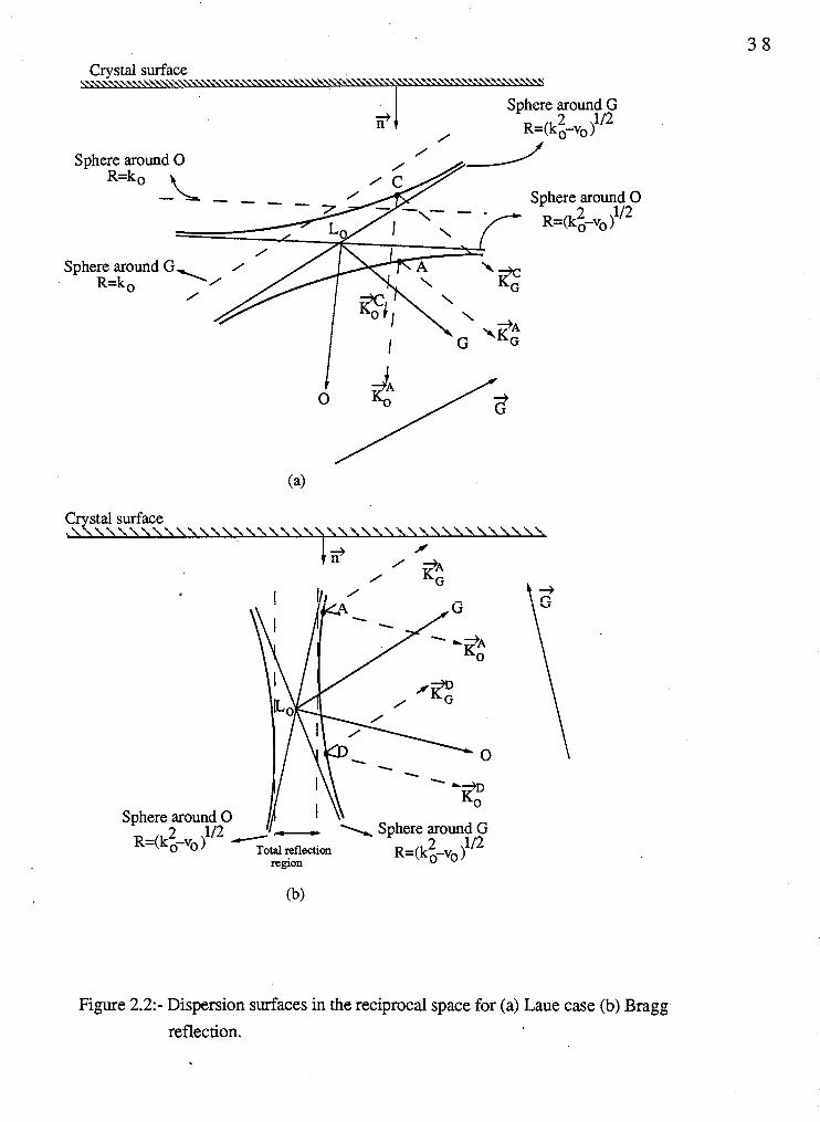
wave vector), are described by two hyperbolae as shown as in Fig. 2.2a (Laue case) and

2.2b (Bragg case). The allowed values of Gz (solutions of eq. 2.1) in the case of the non

extreme asymmetric Laue geometry are given by

and

Similarly, the solutions of eq. (2.3) give the z component of the internal wave vectors in

the case of Bragg geometry. The solutions are

and

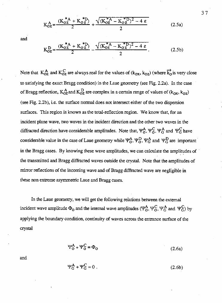
Note that I& and are always real for the values of ( k X , k z ) (where is very close

to satisfying the exact Bragg condition) in the Laue geometry (see Fig. 2.2a). In the case A of Bragg reflection, G Z a n d &% are complex in a certain range of values of (kox, h z )

(see Fig. 2.2b), i.e. the surface normal does not intersect either of the two dispersion

surfaces. This region is known as the total-reflection region. We know that, for an

incident plane wave, two waves in the incident direction and the other two waves in the A C diffracted direction have considerable amplitudes. Note that, Yo, Yo, Y& and YE have

A D A considerable value in the case of Laue geometry while Yo, Yo, Yo and Y!: are important

in the Bragg cases. By howing these wave amplitudes, we can calculate the amplitudes of ' . . the transmitted and Bragg diffracted waves outside the crystal. Note that the amplitudes of

mirror reflections of the incoming wave and of Bragg diffracted wave are negligible in

these non extreme asymmetric Laue and Bragg cases.

In the Laue geometry, we will get the following relations between the external

A C incident wave amplitude Q0 and the internal wave amplitudes (Yo, Yo, Y& and YE) by

applying the boundary condition, continuity of waves across the entrance surface of the

crystal

and

Sphere around G 2 112

0 R=(k ,-v0 )

Suhere around u V , - 2 - 1 \ Sphere around G

CV0 Total reflection R=(ko-v0 2 ) 112 muinn

Figure 2.2:- Dispersion surfaces in the reciprocal space for (a) Laue case (b) Bragg

reflection.

3 9

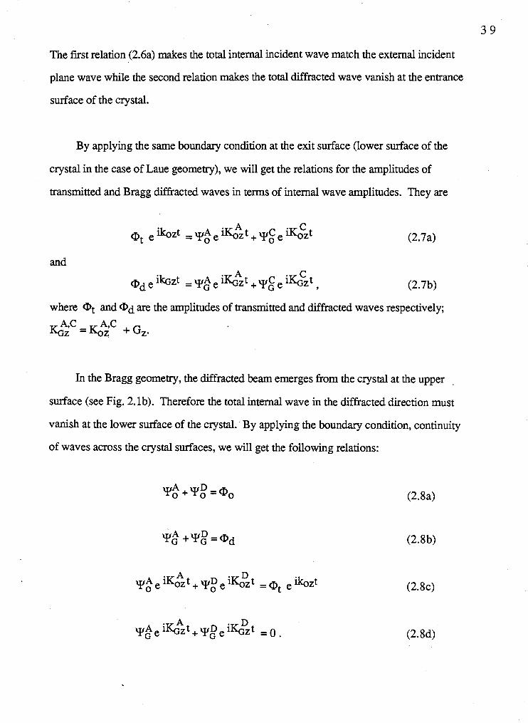
The first relation (2.6a) makes the total internal incident wave match the external incident

plane wave while the second relation makes the total diffracted wave vanish at the entrance

surface of the crystal.

By applying the same boundary condition at the exit surface (lower surface of the

crystal in the case of Laue geometry), we will get the relations for the amplitudes of

transmitted and Bragg diffracted waves in terms of internal wave amplitudes. They are

and

where at and a d are the amplitudes of transmitted and diffracted waves respectively;

In the Bragg geometry, the diffracted beam emerges from the crystal at the upper ,

surface (see Fig. 2.lb). Therefore the total internal wave in the diffracted direction must

vanish at the lower surface of the crystal. By applying the boundary condition, continuity

of waves across the crystal surfaces, we will get the following relations:

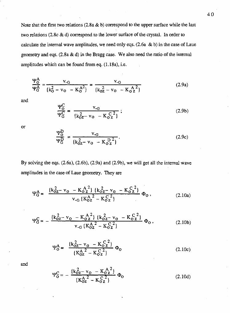
Note that the first two relations (2.8a & b) correspond to the upper surface while the last

two relations (2 .8~ & d) correspond to the lower surface of the crystal. In order to

calculate the internal wave amplitudes, we need only eqs. (2.6a & b) in the case of Laue

geometry and eqs. (2.8a & d) in the Bragg case. We also need the ratio of the internal

amplitudes which can be found from eq. (l.l8a), i.e.

and

By solving the eqs. (2.6a), (2.6b), (2.9a) and (2.9b), we will get all the internal wave

amplitudes in the case of Laue geometry. They are

and

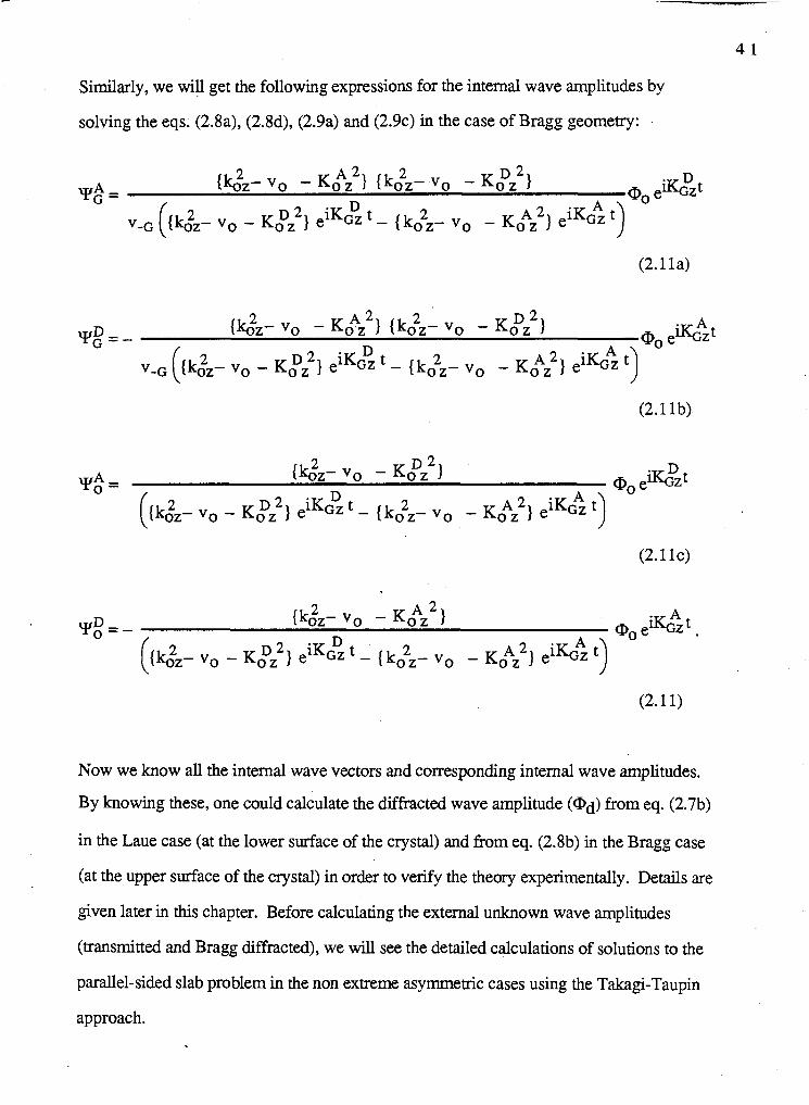
Similarly, we will get the following expressions for the internal wave amplitudes by

solving the eqs. (2.8a), (2.8d), (2.9a) and (2.9~) in the case of Bragg geometry:

(2.1 la)

Now we know all the internal wave vectors and corresponding internal wave amplitudes.

By knowing these, one could calculate the diffracted wave amplitude (ad) from eq. (2.7b)

in the Laue case (at the lower surface of the crystal) and from eq. (2.8b) in the Bragg case

(at the upper surface of the crystal) in order to verify the theory experimentally. Details are

given later in this chapter. Before calculating the external unknown wave amplitudes

(transmitted and Bragg diffracted), we will see the detailed calculations of solutions to the

parallel-sided slab problem in the non extreme asymmetric cases using the Takagi-Taupin

approach.

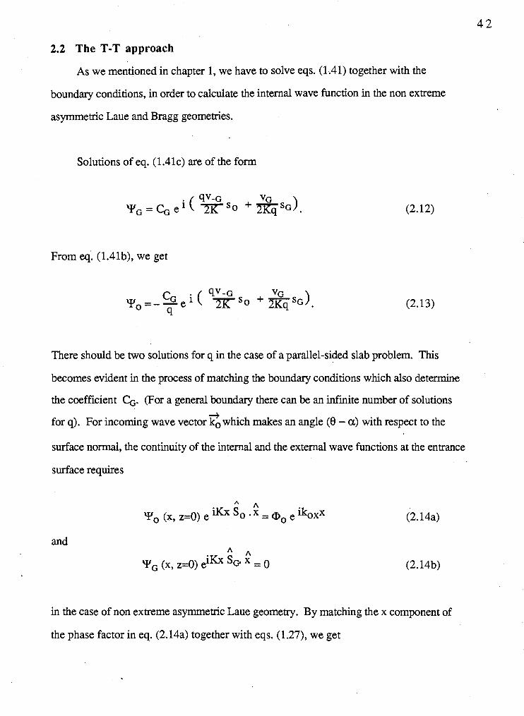
2.2 The T-T approach

As we mentioned in chapter 1, we have to solve eqs. (1.41) together with the

boundary conditions, in order to calculate the internal wave function in the non extreme

asymmetric Laue and Bragg geometries.

Solutions of eq. (1 Ale) are of the form

From eq. (1.41b), we get

There should be two solutions for q in the case of a parallel-sided slab problem. This

becomes evident in the process of matching the boundary conditions which also determine

the coefficient G. (For a general boundary there can be an infinite number of solutions +

for q). For incoming wave vector ko which makes an angle (8 - a) with respect to the

surface normal, the continuity of the internal and the external wave functions at the entrance

surface requires

and

in the case of non extreme asymmetric Laue geometry. By matching the x component of

the phase factor in eq. (2.14a) together with eqs. (1.27), we get

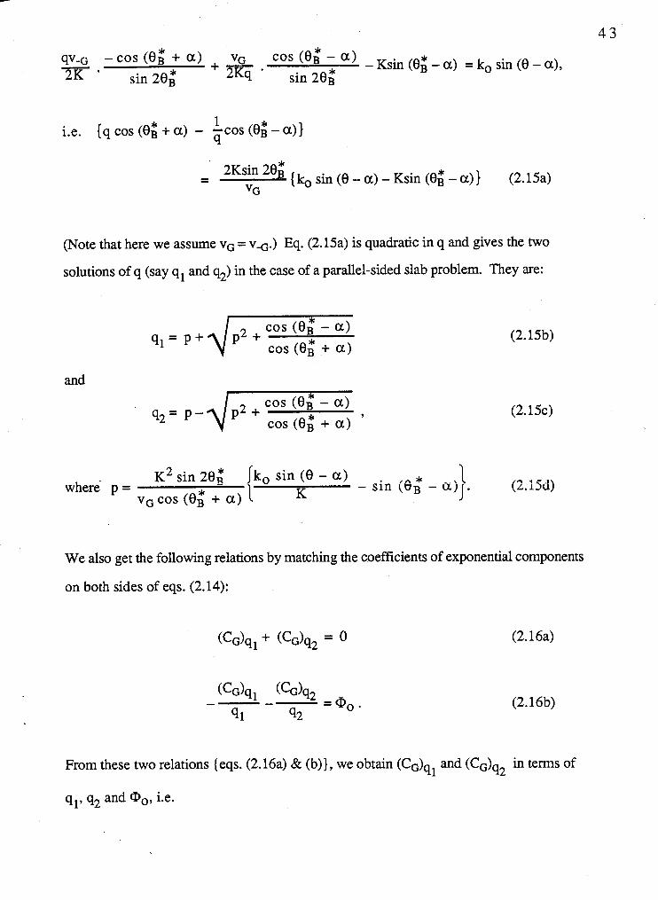
qv-G - cos (0; + a ) VG cos (0; - a) - + - 2Kq ' - Ksin (0; - a) = ko sin (0 - a),

2K ' sin 20; sin 20;

- - 20' { ko sin (0 - a ) - Ksin (0; - a ) } (2.15a) VG

(Note that here we assume vG = v - ~ . ) Eq. (2.15a) is quadratic in q and gives the two

solutions of q (say ql and q2) in the case of a parallel-sided slab problem. They are:

= p + d p 2 + cos (0; - a ) 91 cos (0: + a )

and

cos (8; - a ) q2= P-

cos (0; + a) '

where p = - sin (eB - i)ij ' . (2. 15d) v, cos (0; + a) * I

We also get the following relations by matching the coefficients of exponential components

on both sides of eqs. (2.14):

From these two relations {eqs. (2.16a) & (b)), we obtain (CG)ql and (CG)q2 in terms of

ql, q2 and a?,, i.e.

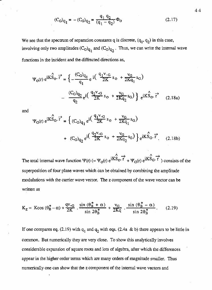
We see that the spectrum of separation constants q is discrete, (ql, q2) in this case,

involving only two amplitudes (CG)a, and (CG)a,, . Thus, we can write the internal wave 1 'L

functions in the incident and the diffracted directions as,

and

x;~.? += The total internal wave function Y(r) (= Yo(r) e + YG@) e i K S ~ . ) consists of the

superposition of four plane waves which can be obtained by combining the arhplitude

modulations with the carrier wave vector. The z component of the wave vector can be

written as

* qv-G sin (8; + a) VG sin (8; - a ) Kz = Kcos (BB - a) + . + - , (2.19) sin 28; 2 K q ' sin28;

If one compares eq. (2.19) with ql and q2 with eqs. (2.4a & b) there appears to be little in

common. But numerically they are very close. To show this analytically involves

considerable expansion of square roots and lots of algebra, after which the differences

appear in the higher order terms which are many orders of magnitude smaller. Thus

numerically one can show that the z component of the internal wave vectors and

corresponding wave amplitudes, which are calculated using both eikonal and T-T

approach, are very nearly equal in the non extreme asymmetric Laue cases. The x

component of the internal wave vectors in both approaches are equal to kox, of course.

The different approximations in both methods create the very small differences in the z

component of the internal wave vectors and in the corresponding wave amplitudes.

Similarly, one could calculate the total internal wave function in the case of Bragg

geometry.

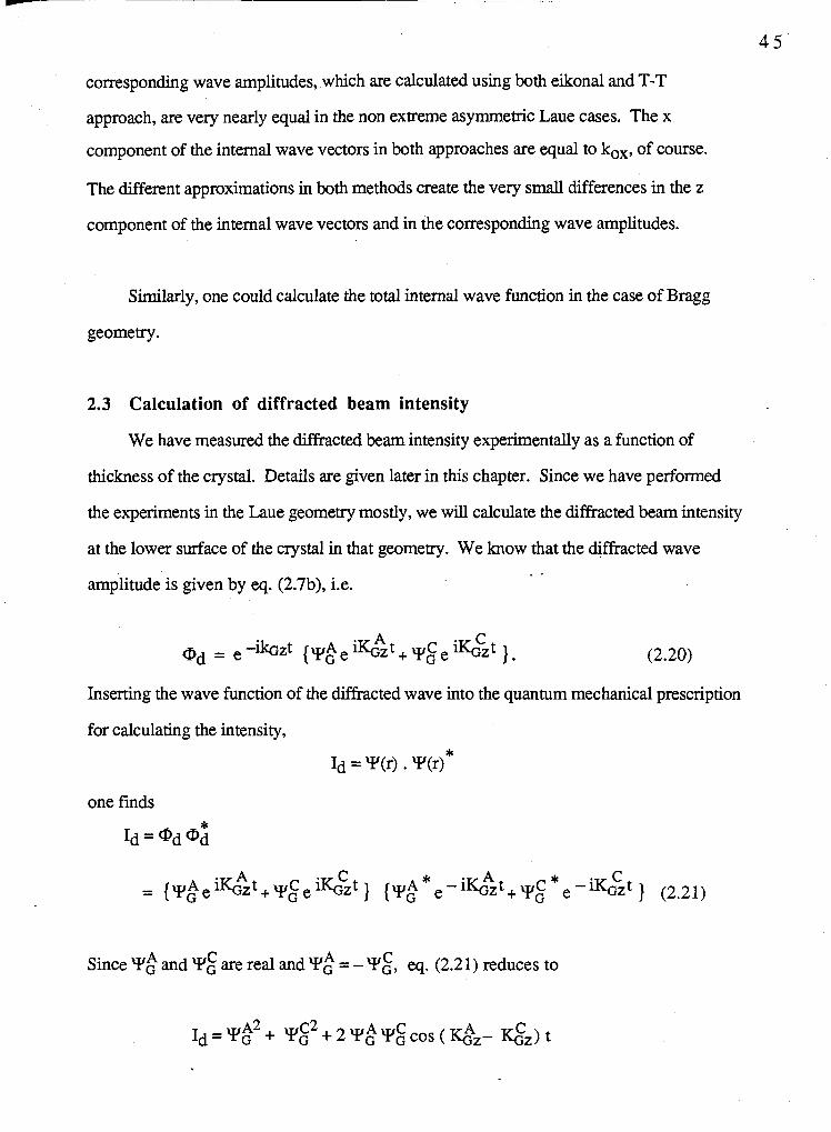
2.3 Calculation of diffracted beam intensity

We have measured the diffracted beam intensity experimentally as a function of

thickness of the crystal. Details are given later in this chapter. Since we have performed

the experiments in the Laue geometry mostly, we will calculate the diffracted beam intensity

at the lower surface of the crystal in that geometry. We know that the diffracted wave - ~

amplitude is given by eq. (2.7b), i.e.

Inserting the wave function of the diffracted wave into the quantum mechanical prescription

for calculating the intensity,

1d = y(r) . ~ ( r ) *

one finds *

Id = @d @d

C Since Y& and YE are real and Y$ = - YG, eq. (2.21) reduces to

A C I ~ = Y & ~ + G z ) t

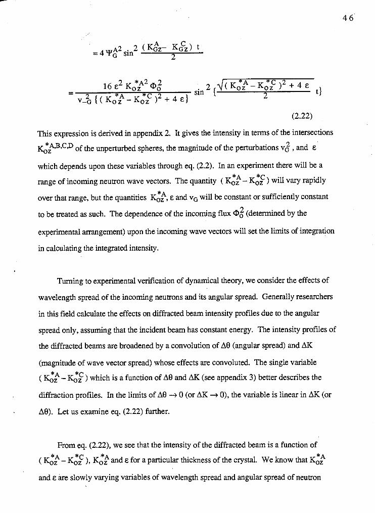
A2 2 ( &- K&) = 4 YG sin 2

2 *~2@, - 16 E KO, 2 ~(K:$K::)~+~E - 2 A 2 sin {

V-G { ( K& -KO*ZC l2 + 4 4 t 1

This expression is derived in appendix 2. It gives the intensity in terms of the intersections

of the unperturbed spheres, the magnitude of the perturbations v z , and E

which depends upon these variables through eq. (2.2). In an experiment there will be a

range of incoming neutron wave vectors. The quantity ( <," - K;Z ) will vary rapidly

over that range, but the quantities d,", E and vc will be constant or sufficiently constant

to be treated as such. The dependence of the incoming flux (determined by the

experimental arrangement) upon the incoming wave vectors will set the limits of integration

in calculating the integrated intensity.

Turning to experimental verification of dynamical theory, we consider the effects of

wavelength spread of the incoming neutrons and its angular spread. Generally researchers

in this field calculate the effects on diffracted beam intensity profiles due to the angular

spread only, assuming that the incident beam has constant energy. The intensity profiles of

the diffracted beams are broadened by a convolution of A8 (angular spread) and AK

(magnitude of wave vector spread) whose effects are convoluted. The single variable

( <,A - KO*: ) which is a function of A8 and AK (see appendix 3) better describes the

diffraction profiles. In the limits of A8 + 0 (or AK O), the variable is linear in AK (or

A8). Let us examine eq. (2.22) further.

From eq. (2.22), we see that the intensity of the diffracted beam is a function of

( K;,A - K:$ ), KZ and E for a particular thickness of the crystal. We know that K,*$

and E are slowly varying variables of wavelength spread and angular spread of neutron

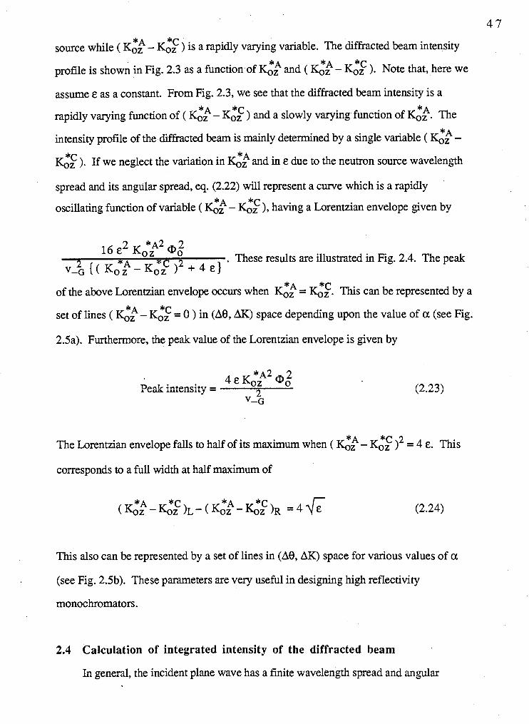
source while ( KcfiA - K:: ) is a rapidly varying variable. The diffracted beam intensity

profile is shown in Fig. 2.3 as a function of Kt$ and ( $& - K:: ). Note that, here we

assume E as a constant. From Fig. 2.3, we see that the diffracted beam intensity is a *c rapidly varying function of ( df - Gz ) and a slowly varying function of K:&. The

intensity profile of the diffracted beam is mainly determined by a single variable ( K:& -

*A Kt: ). If we neglect the variation in Koz and in E due to the neutron source wavelength

spread and its angular spread, eq. (2.22) will represent a curve which is a rapidly

oscillating function of variable ( KG& - d: ), having a Lorentzian envelope given by

2 *~2@, 1 6 8 Koz 2 A . These results are illustrated in Fig. 2.4. The peak

2 + 4 & } v-G { ( K;Z - G Z )

of the above Lorentzian envelope occurs when K:: = <:. This can be represented by a

set of lines ( KG& - IS:: = 0 ) in (Ae, AK) space depending upon the value of a (see Fig.

2.5a). Furthermore, the peak value of the Lorentzian envelope is given by

The Lorentzian envelope falls to half of its maximum when ( d& - IS:: l2 = 4 E. This

corresponds to a full width at half maximum of

This also can be represented by a set of lines in (A8, AK) space for various values of a

(see Fig. 2.5b). These parameters are very useful in designing high reflectivity

monochromators.

2.4 Calculation of integrated intensity of the diffracted beam

In general, the incident plane wave has a fmite wavelength spread and angular

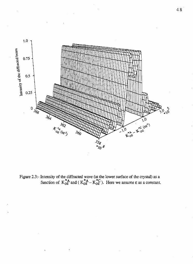
Figure 2.3:- Intensity of the diffracted wave (at the lower surface of the crystal) as a *A *C function of KO, and ( dk - Koz ). Here we assume E as a constant.

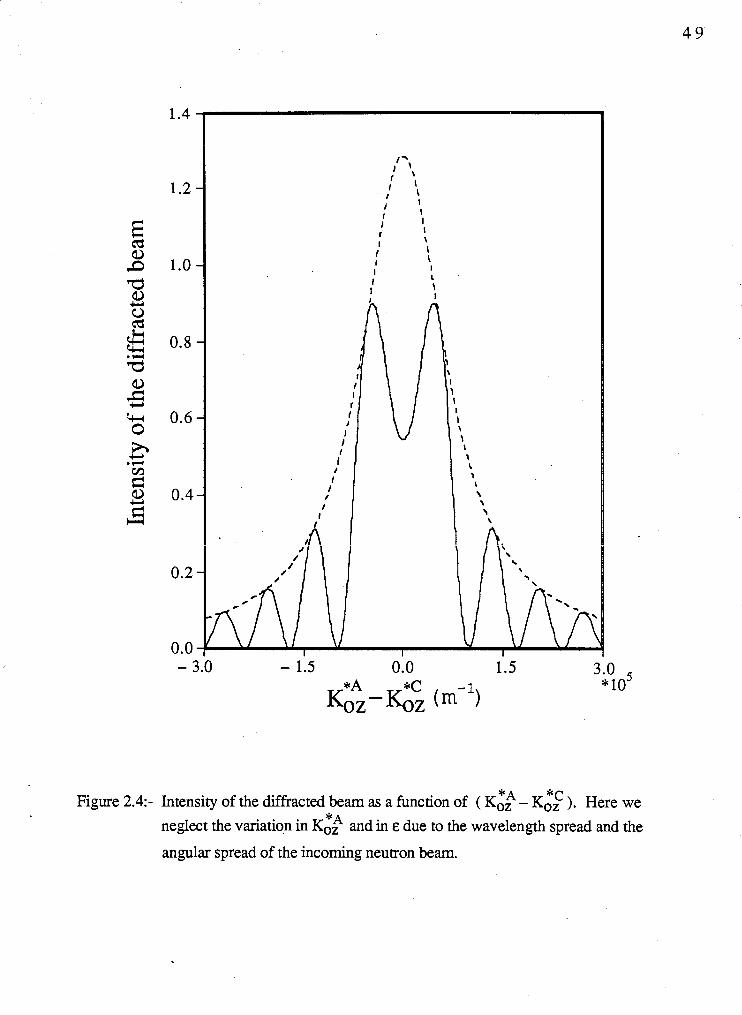
*C Figure 2.4:- Intensity of the diffracted beam as a function of ( K:; - KO, ). Here we

neglect the variation in K:; and in E due to the wavelength spread and the

angular spread of the incoming neutron beam.

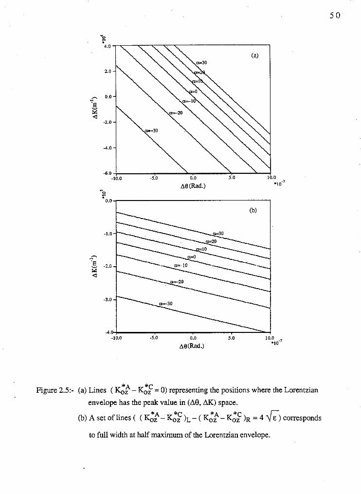
Figure 2.5:- (a) Lines ( g$ - K:: = 0) representing the positions where the Lorentzian

envelope has the peak value in (Ae, AK) space.

*A *C (b) A set of lines ( ( K, - I&,, )L - ( KZ - K:$ )R = 4 6) corresponds

to f d width at half maximum of the Lorentzian envelope.

divergence. So one can represent the incident beam profile by a set of contours in k-space

((k,, kz) plane) depending upon the experimental situations. Therefore, one has to take the

wavelength spread and the angular spread of the incoming beam into account in calculating

the integrated intensity. The integrated intensity of the diffracted beam can be defined as

As we mentioned earlier, the diffracted beam intensity

(2.25)

is a rapidly varying function of

( <$ - 6; ) and a slowly varying function of <,A. One can evaluate the above double

integration (eq. 2.25) by the change of variable method, i.e.

*a - cos (gB + G) where the Jacobian J ( K;e - Gz , I<oz ) -

2 sin eB cos a

(for details see appendix 4).

Substituting the diffracted beam intensity Id {from eq. (2.22)) into eq. (2.26a) we will get,

cos (eB + a) ~(G$-K:$) CI(K;~).

2 sin eB cos a

We see from Fig. 2.3 that the intensity of the diffracted beam decreases rapidly with

increasing or decreasing value of ($2 - KS) from zero. A small spread in wavelength

and in angle of the incoming beam gives a range of values for the variable (K,*," - K:$) in

which the intensity of the diffracted beam has a significant value. For simplicity, we

assume that the incident beam profile is constant over this region. Furthermore the

intensity of the diffracted beam is a slowly varying function of K G ~ over a wide range (see

Fig. 2.3). Therefore one has to take the incident beam profile dependence on into

account in the integrated intensity calculation. The variation of the incident beam profile

with the variable (gk - <$) can be neglected within the range in which the intensity of

the diffracted beam has a significant value. Furthermore, we have neglected also the

variation of E due to the wavelength spread and the angular spread of the incoming

neutrons. With the above assumptions, the double integral {eq. (2.27)) can be split into

two single integrals, i.e.

16 e2 cos (eB + a) I = - I K;*,"".,~(K,*,A)~(K$) v& 2 sin Bg cos a

( K , * , A - K ~ ) ~ + ~ E sin {' r 2 t 1

The second integral is a function of thickness of the crystal (t). The first integral, which is

independent of crystal thickness, is determined by the incident beam profile. For a

particular experimental set up, one could assume that the value of the frst integral is

constant (say C). Then we can rewrite eq. (2.28) as

Our ultimate aim is to calculate the integrated intensity as a function of thickness of the

crystal for several scattering vectors making various angles with respect to the surface of

the crystal. By defining new dimensionless variables

d ( K l k - ~ 2 ) ~ + 4 & V = and T = 6 t , the above equation can be further

reduced to

One can remange this equation in the following form

2 00

I sin €IB cos a sin (VT) dV . 4 E ~ J ~ C O S (eB + a ) c 1 1 = 2 1 7

1+ V ~ V - 1

The right hand side of eq. (2.29) depends only on T (= 6 t ), the normalized crystal

thickness. Now we define I. as the normalized integrated intensity

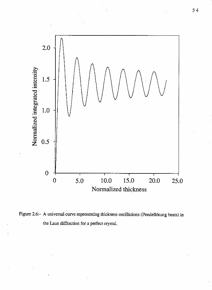
The curve of normalized integrated intensity versus normalized thickness is a universal

curve as shown as in Fig. 2.6. The period of thickness oscillation is 3.102 in normalized

units. From this curve, one can calculate the integrated intensity as a function of thickness

of the crystal for all possible cases of Laue-transmission geometries by multiplying with the

. scaling factors (corresponding to the integrated intensity as well as the thickness of the

crystal). The scaling factors differ from case to case. The period of thickness oscillation is

3.102 e-lR {E-'/' is the characteristic length given by eq. (2.2)) . These results are

verified experimentally and details are given later in this chapter. One has to notice that we

have neglected the variation in E due to the angular spread and the wavelength spread of the

5.0 10.0 15.0 20.0 25.0 Normalized thickness

Figure 2.6:- A universal curve representing thickness oscillations (Pendellbung beats) in

the Laue diffraction for a perfect crystal.

incoming neutrons throughout the integrated intensity calculation. If the portion of incident

beam hitting the sample changes during the process of rotating the crystal sample in order

to examine the different Laue transmission geometries, one would have a different value of

the constant C for different reflections.

2.5 Experimental methods

The experiments were carried out using neutrons (2-5x10~ thermal neutrons1

cm21sec source flux, depending upon how much the proton beam effectiveness is decreased

in the isotope production facility) from the TNF (Thermal Neutron Facility) at TRIUMF.

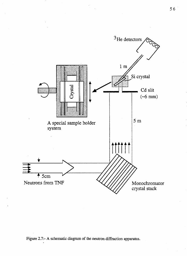
The experimental set up described below is shown in Fig. 2.7. The cross-section of the

thermal neutron beam from the D20 moderator is rectangular with dimensions 5 cm x 20

cm. The beam is monochromated by 90" scattering from the (422) reflection from stacks

of silicon wafers (7.5 cm diameter) which have been specially treated to produce high

reflectivity. This monochromator set up produces neutrons of wavelength =: 1.57 A'. A

cadmium slit of width - 61nm x 20rnm was placed just in front of the sample, 5 m from the

monochromating crystals. The sample crystal was placed on a special sample holder which

was mounted on the spectrometer table. The special sample holder allows one to scan the

crystal from one end to the other using a stepping motor. With this system, one can rotate

the crystal on the table in order to study the asymmetric Laue and Bragg geometries as well

as the symmetric cases. This sample holder is also specially designed for bending the

crystal in a unique manner. Further details are given in chapter 4. The diffracted beam is

detected by a set of 3 ~ e detectors (25 mm diameter by 150 mm) which are placed at a

distance of 1 m from the sample. The detector collects neutrons over a range of 1.75'.

Actually, there are four detectors side by side in our experimental set up. All of the

diffracted neutrons hit one detector while the other three detectors count the background.

These detectors are coupled to a Tennelec electronic counting system. All experimental data

are collected using an IMS computer which also controls the experiment via stepping

motors.

A special sample holder sys tern

I Cd slit (-6 mm)

Figure 2.7:- A schematic diagram of the neutron diffraction apparatus.

A wedge shaped sample was prepared from a dislocation free silicon crystal, the

surface of which was nearly parallel to the (400) direction (004 cut crystal). The Si crystal

was slowly lowered into a bath of planer etch (75% HNO3, 18% Acetic acid and 7% HF)

at a speed of ( XI2 ))Ih. The bath was stirred every half an hour during the etching. After

the fust etch, the thickness of the crystal was measured at different positions along the

translational axis. The thickness of the crystal at the thicker end was 710 pm and at the

thinner end was 480 pm. After neutron studies, the thickness of the crystal was further

decreased by successive etchings. The uniform etch was repeated until the thin edge was

no longer there. The variation of thickness was approximately the same along the

translational axis of the crystal after each etching. The etching is not completely uniform,

so that there are variations of 5 pm at most in thickness across the length (2cm) of the slit.

After each etching the tapered crystal was scanned from one end to the other by moving it

over the Cd slit (6mm width) placed just below the sample mount. The spectrometer was

set to study the (400) reflection (symmetric Laue case) from the Si crystal.

In another set of experiments a (1 11) cut silicon crystal was used. The crystal was

etched as for the above (004) cut crystal except that the edges of the crystal were masked to

prevent etching. This made the etched wafer easier to handle and mount. Only the etched

region was scanned by the slit. Using this sample, the syrnmemc Laue reflection (42) and

asymmetric reflections (In) , (311) and (400) were studied. In the second set of

experiments, the crystal was etched only once.

2.6 Results and Discussion

The experimental curve showing the integrated intensity as a function of thickness for

the (400) symmetric Laue reflection is shown in Fig. 2.8. First we have measured a

rocking curve for each particular thickness of the crystal and the integrated intensity was

calculated by integrating the intensity over the rocking curve. The neutron flux in our

system is low, so that the measurement of each rocking curve took about an hour. The

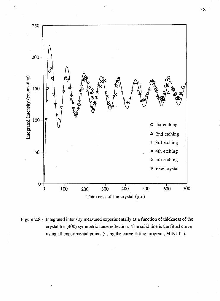
o 1st etching

A 2nd etching

+ 3rd etching

x 4th etching

o 5th etching

V new crystal

Thickness of the crystal (pm)

Figure 2.8:- Integrated intensity measured experimentally as a function of thickness of the

crystal for (400) symmetric Laue reflection. The solid line is the fitted curve

using all experimental points (using the curve fitting program, MINUIT).

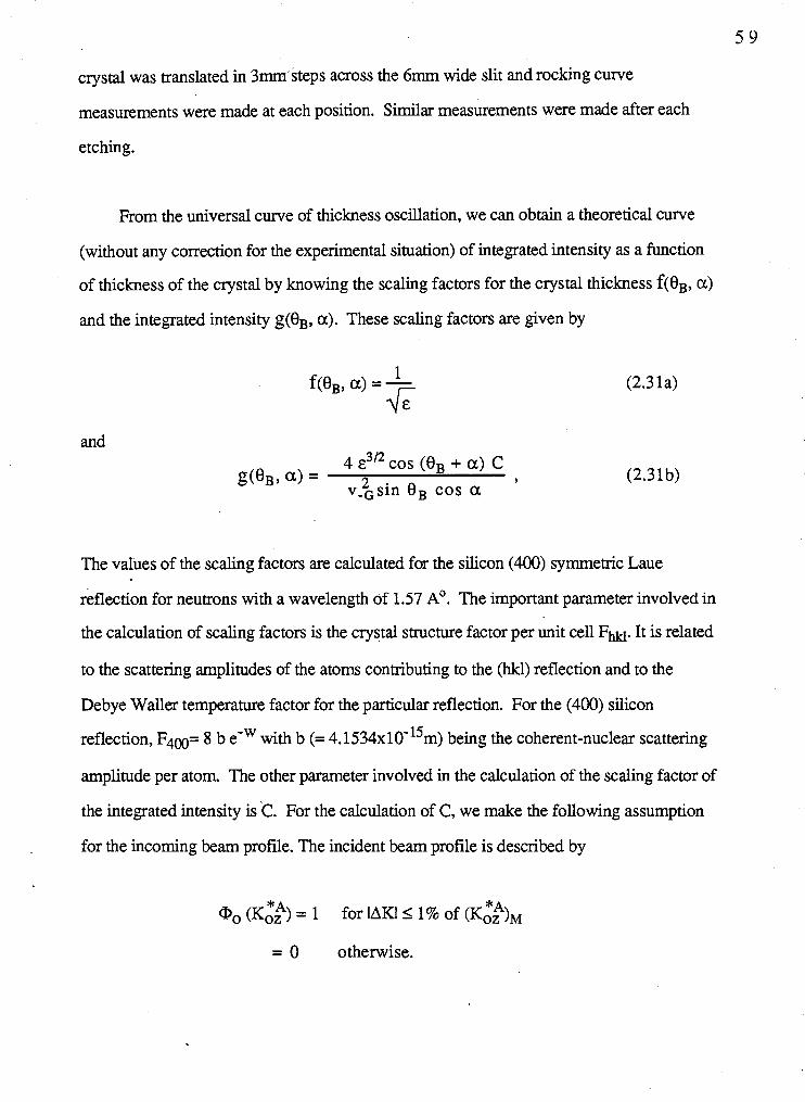
crystal was translated in 3- steps across the 6mm wide slit and rocking curve

measurements were made at each position. Similar measurements were made after each

etching.

From the universal curve of thickness oscillation, we can obtain a theoretical curve

(without any correction for the experimental situation) of integrated intensity as a function

of thickness of the crystal by knowing the scaling factors for the crystal thickness f(eB, a)

and the integrated intensity g(eB9 a). These scaling factors are given by

and 4 e3I2 cos (eB + a ) C

ge , , a ) = 2 sin eB cos a 9

The values of the scaling factors are calculated for the silicon (400) symmetric Laue

reflection for neutrons with a wavelength of 1.57 A". The important parameter involved in

the calculation of scaling factors is the crystal structure factor per unit cell Fhkl. It is related

to the scattering amplitudes of the atoms contributing to the (hkl) reflection and to the

Debye Waller temperature factor for the particular reflection. For the (400) silicon

reflection, F 4 ~ = 8 b e-W with b (= 4.1534~10-~~m) being the coherent-nuclear scattering

amplitude per atom. The other parameter involved in the calculation of the scaling factor of

the integrated intensity is C. For the calculation of C, we make the following assumption

for the incoming beam profile. The incident beam profile is described by

"A ( K ) = 1 for IAKI 5 1% of (KO, ),

= 0 otherwise.

6 0

where K:; = (K::)~ + AK and (&&,l is the value of 6: at the exact Bragg condition

for ko = 4 x 10'~m-' (h = 1.57 A'). With this assumption the value of C is equal to

6.942x10*~(m-') for the (400) symmetric Laue reflection. The calculated values of the

scaling factors are 2.66x10-~(m) and 3.457~10'~(m-~) for the crystal thickness and for the

integrated intensity using the above parameters.

Next we will consider the corrections for the experimental situation. During the

experiment we have placed a 6 mm wide Cd slit across the incoming beam. So one has to

consider the effects of the slit in the intensity calculation. However, there won't be any

correction in the total integrated intensity by introducing the slit across the incident beam.

Now we will justify this statement.

We consider the geometry as shown in Fig. 2.9. Let Wo (=2a) be the width of the

slit AB. The incoming neutrons impinge on the entrance surface of the crystal along a strip

A'B' of width Wi { = 2a/cos (&a) = 2a/cos (eB-a)) due to the presence of the slit AB.

The origin is chosen to be at the center of A'B'. By introducing the slit AB across the

incident beam, we will get non-zero wave fields in the segment CF at the lower surface of

the crystal. The width of the segment CF (W) is related to the width of the strip A'B' (Wi )

and the thickness of the crystal by

As we see from Fig. 2.9, any point in the region DE receives the same neutron flux as it

would if the slit were infinitely wide, i.e. the points in the region DE covers a complete

inverse Borrmann triangle. At the same time, the points in the regions CD and EF receive

only a part of the plane wave intensity. Therefore the wave field is constant on the segment

DE and is found as the solution of the ordinary dynamic problem (Plane wave type

approximation). The width of the segment DE (Wd) is given by

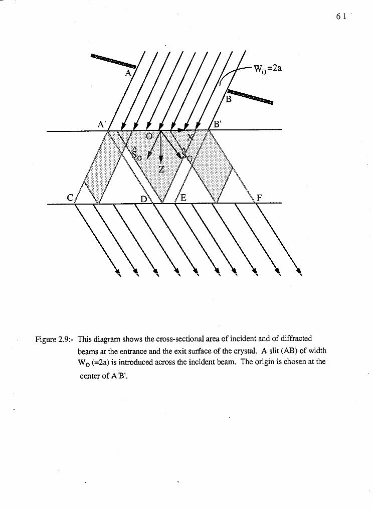
Figure 2.9:- This diagram shows the cross-sectional area of incident and of diffracted

beams at the entrance and the exit surface of the crystal. A slit (AB) of width Wo (=2a) is introduced across the incident beam. The origin is chosen at the

center of A'B'.

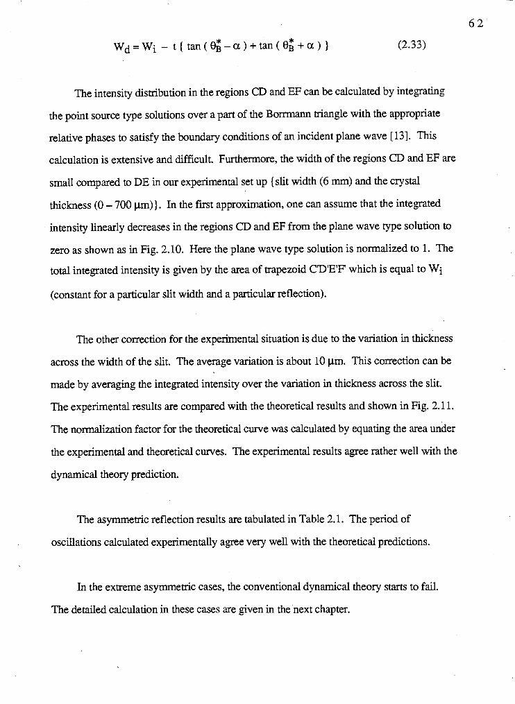
The intensity distribution in the regions CD and EF can be calculated by integrating

the point source type solutions over a part of the Borrrnann triangle with the appropriate

relative phases to satisfy the boundary conditions of an incident plane wave [13]. This

calculation is extensive and difficult. Furthermore, the width of the regions CD and EF are

small compared to DE in our experimental set up {slit width (6 mm) and the crystal

thickness (0 - 700 pm)). In the fnst approximation, one can assume that the integrated

intensity linearly decreases in the regions CD and EF from the plane wave type solution to

zero as shown as in Fig. 2.10. Here the plane wave type solution is normalized to 1. The

total integrated intensity is given by the area of trapezoid C'D'E'F' which is equal to Wi

(constant for a particular slit width and a particular reflection).

The other correction for the experimental situation is due to the variation in thickness

across the width of the slit. The average variation is about 10 ym. This correction can be

made by averaging the integrated intensity over the variation in thickness across the slit.

The experimental results are compared with the theoretical results and shown in Fig. 2.1 1.

The normalization factor for the theoretical curve was calculated by equating the area under

the experimental and theoretical curves. The experimental results agree rather well with the

dynamical theory prediction.

The asymmetric reflection results are tabulated in Table 2.1. The period of

oscillations calculated experimentally agree very well with the theoretical predictions.

In the extreme asymmetric cases, the conventional dynarnical theory starts to fail.

The detailed calculation in these cases are given in the next chapter.

Figure 2.10:- This diagram illustrates the integrated intensity as a function of position

at the exit surface of the crystal. The integrated intensity in the segment DE

(plane wave type solution) is normalized to 1.

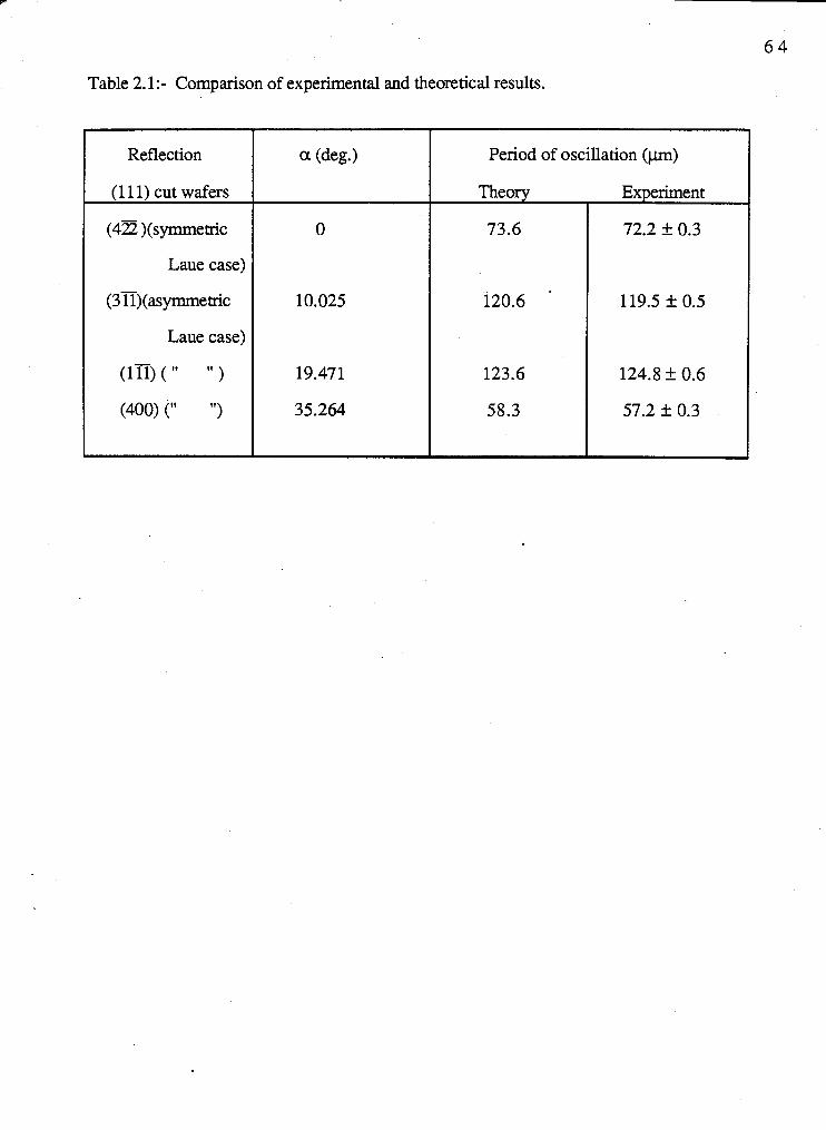
Table 2.1:- Comparison of experimental and theoretical results.

Reflection

(1 11) cut wafers

( 4 2 )(symmetric

Laue case)

(3ii)(asyrnmetric

Laue case)

(111) ( " " )

(400) (" ")

Period of oscillation (pm)

Theory Experiment

72.2 + 0.3

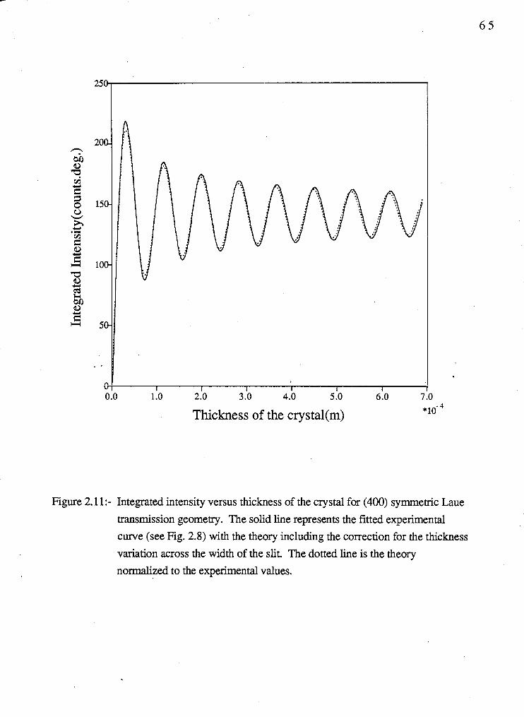
Thickness of the crystal(m) *lo-

Figure 2.11:- Integrated intensity versus thickness of the crystal for (400) symmemc Laue

transmission geometry. The solid line represents the fitted experimental

curve (see Fig. 2.8) with the theory including the correction for the thickness

variation across the width of the slit. The dotted line is the theory

normalized to the experimental values.

CHAPTER 3

EXTENDED THEORY OF DIFFRACTION

3.1 Introduction

The conventional dynamical theory of neutron diffraction, which works very well in

both symmetric and non extreme asymmetric Laue and Bragg cases, is not valid in extreme

asymmetric cases of Laue and Bragg geometries. In the conventional theory, the

dispersion surface is approximated to hyperboloids and the asymptotes of the dispersion

surfaces are straight lines. In general, the dispersion surface is described by an equation of

the fourth order. This fourth order equation can be reduced to a second order equation in

symmetric and non extreme asymmetric Laue and Bragg cases, because the distance

between the Laue point and only two of the four tie points is small. Therefore, only the

wave field corresponding to these two tie points have considerable amplitudes and only

they have to be known accurately. Note that the wave field corresponding to each tie point

consists of two waves, one in the incident direction and the other in the diffracted Ciirectbii.

However, in the extreme asymmetric cases, the distance between the Laue point and at least

three tie points is small and three wave fields associated with these three tie points become

important. In addition, there are four waves appearing out side the crystal (besides the

incident wave) instead of two in the symmetric and non extreme asymmetric cases. They

are the transmitted wave, the Bragg diffracted wave and the mirror reflections of the

incident and of the diffracted wave (specular reflected wave and specular diffracted wave).

There are four possible extreme asymmetric cases, depending on which beam

(incident or diffracted beam) makes a small angle with the crystal surface and whether the

geometry is Laue or Bragg. These extreme asymmetric cases of x-ray diffraction were

studied extensively using some approximations by different groups. Kishino and Kohra

[14], Briimmer et. al. [15, 161 and Zeilinger and Beatty [17] treated an extreme asymmetric

Bragg case in which the angle between the incident beam and the crystal surface is small.

Kishino [18] and ~ e n ~ & k a [19] investigated the Bragg case with a small angle between

the crystal surface and their diffracted beam. The diffraction patterns in extremely

asymmetric Laue cases were studied in the papers by Kishino et. al. [20], ~ e n ~ d s k a

[19,21] and H&twig [22,23].

In this chapter, four extreme asymmetric cases of neutron diffraction are investigated.

In these cases, at most three tie points are close to the Laue point. One tie point is always

far away from the Laue point. Therefore one can use the asymptotic value for the wave

vector corresponding to this tie point. In addition, the amplitudes of the internal wave field

associated with this tie point are extremely small. With this assumption, we can reduce the

fourth order equation of dispersion to a cubic equation. The solution of a cubic equation is

straight forward. The solutions of this cubic equation will give accurate values of the wave

vectors associated with the three tie points. Furthermore, either the specular reflected wave

or the specui& diffracted wave will have a considerable amplitude in the extreme

asymmetric cases depending on which beam, either the incident beam or the diffracted

beam makes, a small angle with the crystal surface. The unknown internal and external

wave amplitudes can be calculated by applying the boundary conditions at the upper and

lower surfaces of the crystal. The results are discussed in this chapter in great detail for all

extreme asymmetric cases. The results are also compared with the conventional theory.

3.2 Theoretical formulation

We consider the diffraction geometry schematically shown in Fig. 3.1, for the Laue

case. Diffraction takes place from the lattice planes (hkl) making an angle a with the

inward crystal normal. In this particular case, the angle between the incident beam and the

crystal surface is small (comparable to the critical angle of specular reflection ec). Note

that, theoretically one can obtain the other extreme asymmetric cases by changing the value

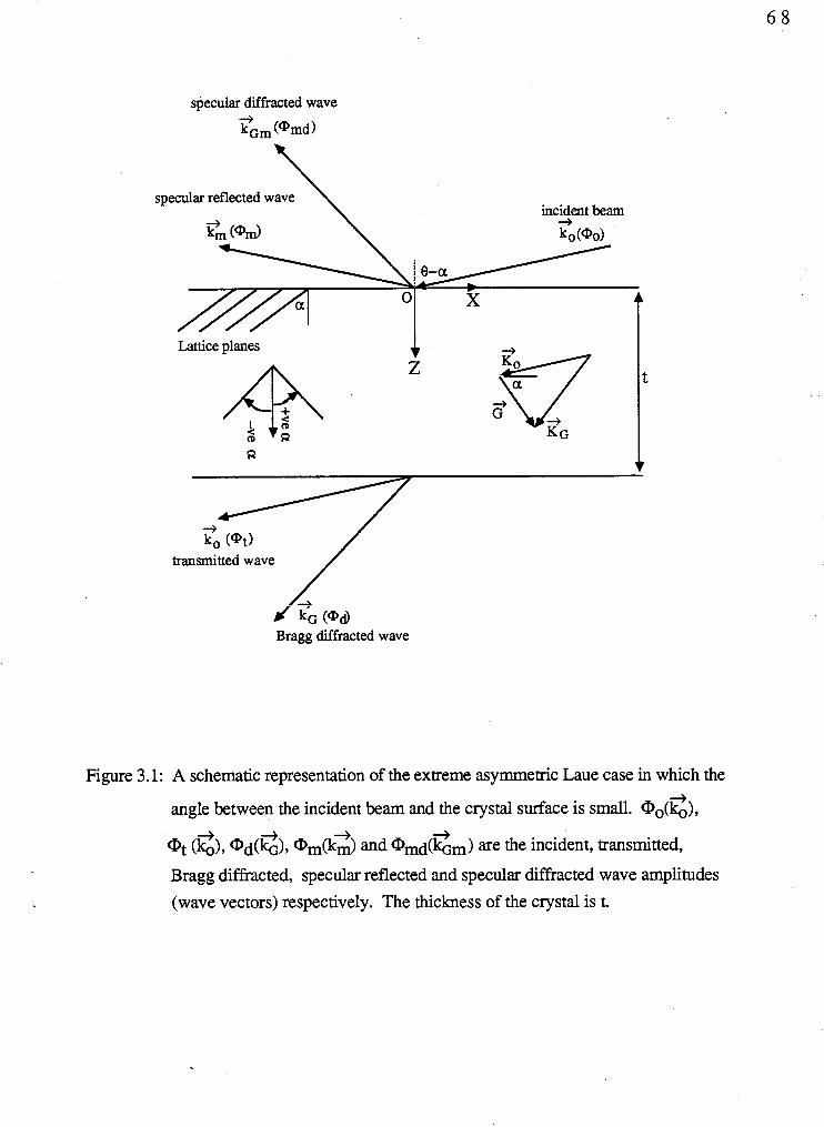
specular diacted wave -+ kGm (amdl

specular reflected wave \ incident beam

transmitted wave /

Bragg diffracted wave

Figure 3.1: A schematic representation of the extreme asymmetric Laue case in which the

angle between the incident beam and the crystal surface is small. a o ( z ) , 7' at (s), o ~ ( G ) , am(k2) and Qmd(bm) are the incident, transmitted,

Bragg diffracted, specular reflected and specular diffracted wave amplitudes

(wave vectors) respectively. The thickness of the crystal is t.

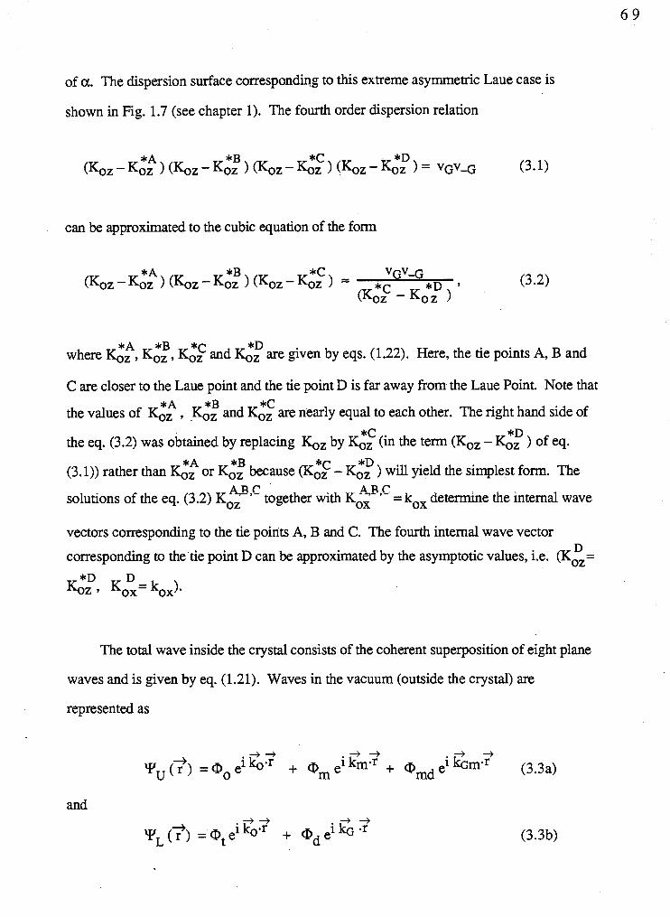
of a. The dispersion surface corresponding to this extreme asymmetric Laue case is

shown in Fig. 1.7 (see chapter 1). The fourth order dispersion relation

can be approximated to the cubic equation of the form

*A *B *C *D where KO, , KO, , KO, and Gz are given by eqs. (1.22). Here, the tie points A, B and

C are closer to the Laue point and the tie point D is far away from the Laue Point. Note that *A *B *C

the values of GZ , .Gz and Gz are nearly equal to each other. The right hand side of *C *D

the eq. (3.2) was obtained by replacing GZ by GZ (in the term ( G Z - Koz ) of eq. *A *B *D

(3.1)) rather than Gz or Koz because (K:: - GZ ) will yield the simplest form. The A E,C solutions of the eq. (3.2) K&?" together with KO,' = kox determine the internal wave

vectors corresponding to the tie points A, B and C. The fourth internal wave vector D corresponding to the tie point D can be approximated by the asymptotic values, i.e. (K,,=

The total wave inside the crystal consists of the coherent superposition of eight plane

waves and is given by eq. (1.21). Waves in the vacuum (outside the crystal) are

represented as

and

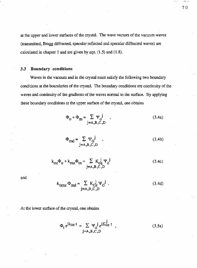
at the upper and lower surfaces of the crystal. The wave vectors of the vacuum waves

(transmitted, Bragg diffracted, specula. reflected and specular diffracted waves) are

calculated in chapter 1 and are given by eqs. (1.5) and (1.8).

3.3 Boundary conditions

Waves in the vacuum and in the crystal must satisfy the following two boundary

conditions at the boundaries of the crystal. The boundary conditions are continuity of the

waves and continuity of the gradients of the waves normal to the surface. By applying

these boundary conditions at the upper surface of the crystal, one obtains

and

At the lower surface of the crystal, one obtains

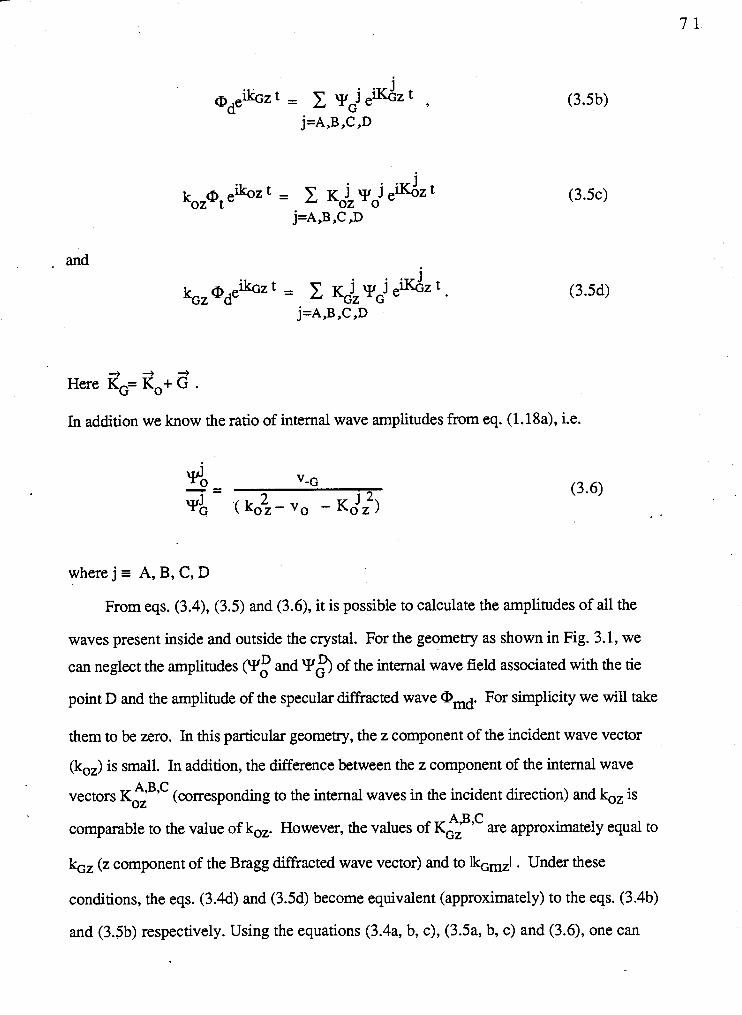
. and

+ + + Here KG= KO+ G .

In addition we know the ratio of internal wave amplitudes from eq. (1.18a), i.e.

wherej z A,B, C,D

From eqs. (3.4), (3.5) and (3.6), it is possible to calculate the amplitudes of all the

waves present inside and outside the crystal. For the geometry as shown in Fig. 3.1, we

can neglect the amplitudes (Y," and Y G ~ of the internal wave field associated with the tie

point D and the amplitude of the specular diffracted wave am& For simplicity we will take

them to be zero. In this particular geometry, the z component of the incident wave vector

(ko,) is small. In addition, the difference between the z component of the internal wave

(corresponding to the internal waves in the incident direction) and ko, is vectors KO,

are approximately equal to comparable to the value of ko,. However, the values of KGz

bZ (Z component of the Bragg diffracted wave vector) and to IbmzI . Under these

conditions, the eqs. (3.4d) and (3.5d) become equivalent (approximately) to the eqs. (3.4b)

and (3.5b) respectively. Using the equations (3.4a, b, c), (3.5a, b, c) and (3.6), one can

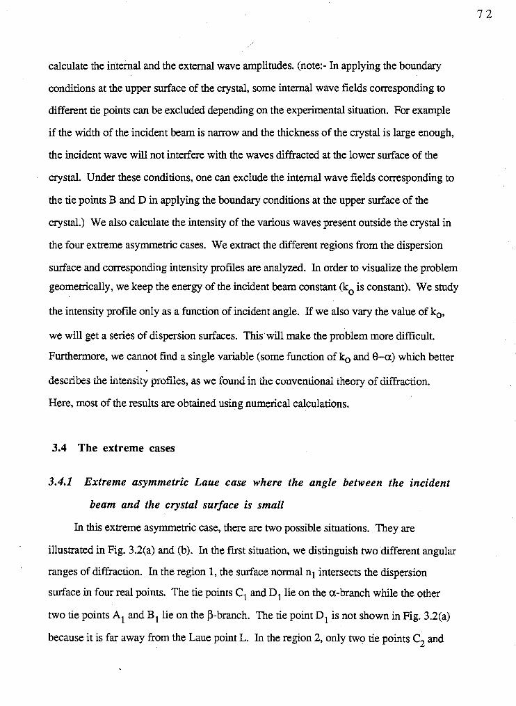
calculate the internal and the external wave amplitudes. (note:- In applying the boundary

conditions at the upper surface of the crystal, some internal wave fields corresponding to

different tie points can be excluded depending on the experimental situation. For example

if the width of the incident beam is narrow and the thickness of the crystal is large enough,

the incident wave will not interfere with the waves diffracted at the lower surface of the

crystal. Under these conditions, one can exclude the internal wave fields corresponding to

the tie points B and D in applying the boundary conditions at the upper surface of the

crystal.) We also calculate the intensity of the various waves present outside the crystal in

the four extreme asymmetric cases. We extract the different regions from the dispersion

surface and corresponding intensity profiles are analyzed. In order to visualize the problem

geometrically, we keep the energy of the incident beam constant (ko is constant). We study

the intensity profile only as a function of incident angle. If we also vary the value of ko,

we will get a series of dispersion surfaces. This will make the problem more difficult.

Furthermore, we cannot find a single variable (some function of k, and 9-a) which better

describes the intensity profiles, as we found in the conventional theory of diffraction.

Here, most of the results are obtained using numerical calculations.

3.4 The extreme cases

3.4.1 Extreme asymmetric Laue case where the angle between the incident

beam and the crystal surface is small

In this extreme asymmetric case, there are two possible situations. They are

illustrated in Fig. 3.2(a) and (b). In the first situation, we distinguish two different angular

ranges of diffraction. In the region 1, the surface normal nl intersects the dispersion

surface in four real points. The tie points C1 and Dl lie on the a-branch while the other

two tie points Al and B1 lie on the kbranch. The tie point Dl is not shown in Fig. 3.2(a)

because it is far away from the Laue point L. In the region 2, only two tie points C2 and

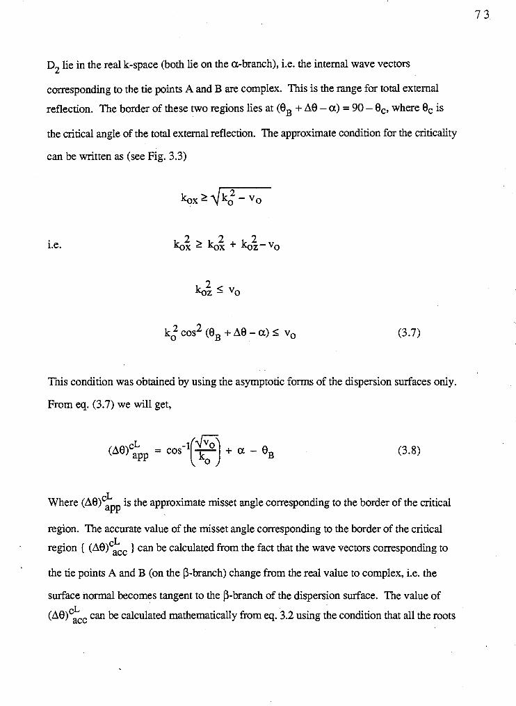
D2 lie in the real k-space (both lie on the a-branch), i.e. the internal wave vectors

corresponding to the tie points A and B are complex. This is the range for total external

reflection. The border of these two regions lies at (Bg + A0 - a ) = 90 - Bc, where €Ic is

the critical angle of the total external reflection. The approximate condition for the criticality

can be written as (see Fig. 3.3)

2 2 2 kox 2 kox + bz- vo

2 2 ko cos (BB + A0 - a ) 5 vo

. . - . lnis condition was obtained by using the asymptotic forms of the dispersion surfaces oniy.

From eq. (3.7) we will get,

Where ( ~ 0 ) ~ : ~ ~ is the approximate misset angle corresponding to the border of the critical

region. The accurate value of the misset angle corresponding to the border of the critical

region { (~0)';~ } can be calculated from the fact that the wave vectors corresponding to

the tie points A and B (on the P-branch) change from the real value to complex, i.e. the

surface normal becomes tangent to the P-branch of the dispersion surface. The value of

( A B ) C ~ can be calculated mathematically from eq. 3.2 using the condition that all the roots

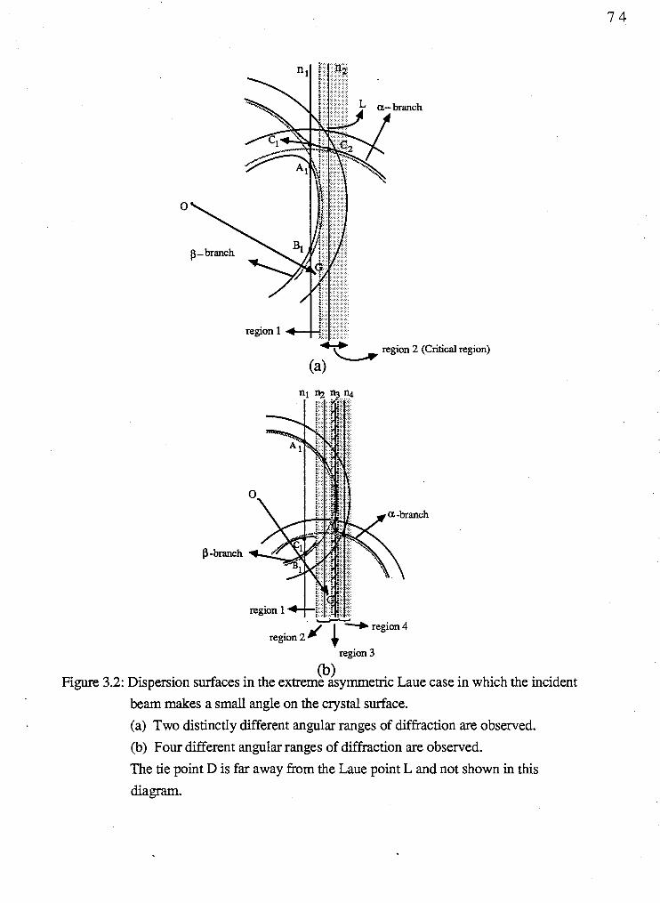
branch

-- region 2 (Critical region)

(a)

;w ---) region 4

region 2 J & region 3

0) Figure 3.2: Dispersion surfaces in the extreme asymmetric Laue case in which the incident

beam makes a small angle on the crystal surface.

(a) Two distinctly different angular ranges of diffraction are observed.

(b) Four different angular ranges of diffraction are observed.

The tie point D is far away from the Laue point L and not shown in this

diagram.

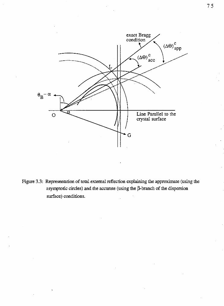
Line Parallel to the crystal surface

Figure 3.3: Representation of total external reflection explaining the approximate (using the asymptotic circles) and the accurate (using the fl-branch of the dispersion

surface) conditions.

of that cubic equation (eq. 3.2) have to be real and at least two are equal. aPP ' (AO)C.&~ and the difference between these two values - ( ~ 0 ) ~ ; ~ ) are plotted

aPP

against (BB - a ) in Fig. 3.4.

In the second situation {Fig. 3.2(b)), we distinguish four different angular regions of

diffraction. In the region 1, we excite four real tie points in a same way as in the region 1

of the f is t situation. In the region 2, we excite only two real tie points (both lie on the a-

branch). If we decrease the angle of incidence, we are in a situation such that the surface

normal n3 again cut the dispersion surface in four real points (region 3). These four tie

points are now arranged on the a-branch of the dispersion surface. We excite only two

real tie points in the region 4.

In Fig. 3.2(b), the incident beam corresponding to the exact Bragg condition would

have to be inside the crystal, i.e. BB - a > 90'. However, the incident beams which

produce the four different angular ranges of diffraction (see Fig. ?.2(b)) have finite misset

angles and can be outside the crystal surface, making small angles with the crystal surface.

It is clear that these two situations {Fig. 3.2(a) & (b)) are well separated by a condition in

which the surface normal becomes tangent to the a-branch of the dispersion surface at the

inflection point of that branch. For a particular value of G, this condition is determined by

the values of k, and a , i.e. if we fixed the orientation of the reflecting planes with respect

to the inward surface normal (a), the condition will occur at a particular value of k, (kb) or

if we fixed k,, the condition will occur at a particular value of a (a!$. Note that this

condition occurs only when BB - a > 90'. We will get either the f i s t or the second

situation depending upon the value of k, (a) which is slightly greater than or less than kk

(4) for the fixed values of a (k,) and G.

In this particular extreme asymmetric case, the amplitude of the specula reflected

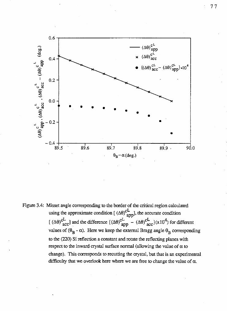
8, - a (deg.)

Figure 3.4: Misset angle corresponding to the border of the critical region calculated

using the approximate condition [ ( ~ 0 ) ' ~ 1, the accurate condition aPP

[ (AB)C;~] and the difference { ( A B ) C ~ ~ ~ - ( A € ~ ) C ~ ~ ) ( X ~ O ~ ) for different

values of (BB - a). Here we keep the external Bragg angle eB corresponding

to the (220) Si reflection a constant and rotate the reflecting planes with respect to the inward crystal surface normal (allowing the value of a to

change). This corresponds to recutting the crystal, but that is an experimental difficulty that we overlook here where we are free to change the value of a.

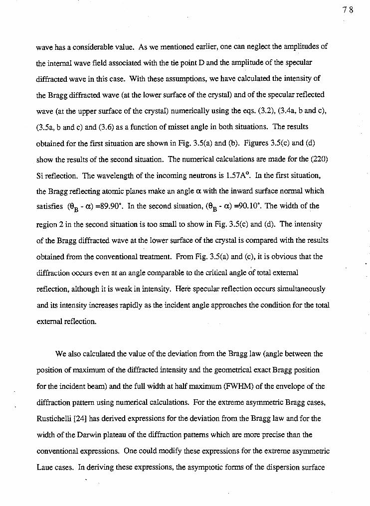
wave has a considerable value. As we mentioned earlier, one can neglect the amplitudes of

the internal wave field associated with the tie point D and the amplitude of the specular

diffracted wave in this case. With these assumptions, we have calculated the intensity of

the Bragg diffracted wave (at the lower surface of the crystal) and of the specular reflected

wave (at the upper surface of the crystal) numerically using the eqs. (3.2), (3.4a, b and c),

(3.5a, b and c) and (3.6) as a function of misset angle in both situations. The results

obtained for the first situation are shown in Fig. 3.5(a) and (b). Figures 3.5(c) and (d)

show the results of the second situation. The numerical calculations are made for the (220)

Si reflection. The wavelength of the incoming neutrons is 1.57A0. In the first situation,

the Bragg reflecting atomic planes make an angle a with the inward surface normal which

satisfies (BB - a ) =89.90•‹. In the second situation, (BB - a) =90.10•‹. The width of the

region 2 in the second situation is too small to show in Fig. 3.5(c) and (d). The intensity

of the Bragg diffracted wave at the lower surface of the crystal is compared with the results

obtained from the conventional treatment. From Fig. 3.5(a) and (c), it is obvious that the

biffiactisn occurs even at an angle cornpafable to the ~witical angle of total external

reflection, although it is weak in intensity. Here specular reflection occurs simultaneously

and its intensity increases rapidly as the incident angle approaches the condition for the total

external reflection.

We also calculated the value of the deviation from the Bragg law (angle between the

position of maximum of the diffracted intensity and the geometrical exact Bragg position

for the incident beam) and the full width at half maximum (FWHM) of the envelope of the

diffraction pattern using numerical calculations. For the extreme asymmetric Bragg cases,

Rustichelli [24] has derived expressions for the deviation from the Bragg law and for the

width of the Darwin plateau of the diffraction patterns which are more precise than the

conventional expressions. One could modify these expressions for the extreme asymmetric

Laue cases. In deriving these expressions, the asymptotic forms of the dispersion surface

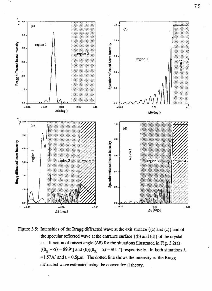
- 0.20

A9 (deg.)

region 1

0.00

A 9 (deg.)

Figure 3.5: Intensities of the Bragg diffracted wave at the exit surface ((a) and (c)) and of

the specular reflected wave at the entrance surface {(b) and (d)) of the crystal as a function of misset angle (A8) for the situations illustrated in Fig. 3.2(a) [(e, - a ) = 89.9'1 and (b)[(BB - a) = 90.1'1 respectively. In both situations h

=1.57A0 and t = 0.5pm. The dotted line shows the intensity of the Bragg

diffracted wave estimated using the conventional theory.

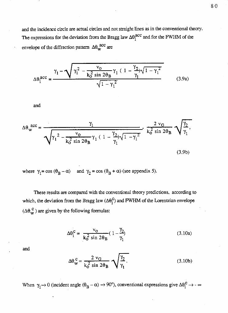
and the incidence circle are actual circles and not straight lines as in the conventional theory.

The expressions for the deviation from the Bragg law Aeiacc and for the FWHM of the

envelope of the diffraction pattern AB? are

vo y l . \ I ~ : - sin 2eB Y1 ( 1 - % / - -

~ 0 . y = % (3.9a)

+7

and

where yl= cos (eB - a) and y2 = cos (BB + a) (see appendix 5).

These results are compared with the conventional theory predictions, according to

which, the deviation from the Bragg law (A8f) and FWHM of the Lorentzian envelope

(88; ) are given by the following formulas:

and

When yl+ 0 (incident angle (OB - a) + 90•‹), conventional expressions give A0f -t - -

and A 8 4 + -. Rustichelli's modified expressions give Aeiacc + -

A 8 F + 0 as yl + 0. We see that the conventional expressions start to fail as yl

approaches to zero. Results obtained from these three approaches are graphically shown in

Figs. 3.6(A) and (B). The numerical values calculated using the present theory (extended

theory) agree with Rustichelli's curves representing the deviation from the Bragg law and

the FWHM of the envelope of the diffraction pattern.

3.4.2 Extreme asymmetric Laue case where the angle between the Bragg

diffracted beam and the crystal surface is small

In this extreme asymmetric Laue case, it is possible to distinguish three different

angular ranges of diffraction (see Fig. 3.7). In the range 1, the surface normal nl intersects

the dispersion surface in four real points; C1 and B lie on the a-branch, Al and D lie on

the ebranch. Here the tie point B1 is far away from the Laue point L and it is not shown

in Fig. 3.7. In the range 2, only two tie points A2 and B2 (both on the a-branch) lie in the

real k-space. In the range 3, the tie points Ag and Bg lie in the real k-space. In addition,

bz and bmz (Z components of the wave vectors of the Bragg diffracted and of the

specular diffracted waves) are purely imaginary in this region, i.e. the phenomenon of total

internal reflection of the diffracted wave occurs.

The approximate misset angle corresponding to the border of the regions 1 and 2

[(Ae)iPp] can be calculated from the following condition:

K;; = K*D = - G, , oz (see Fig 3.8)

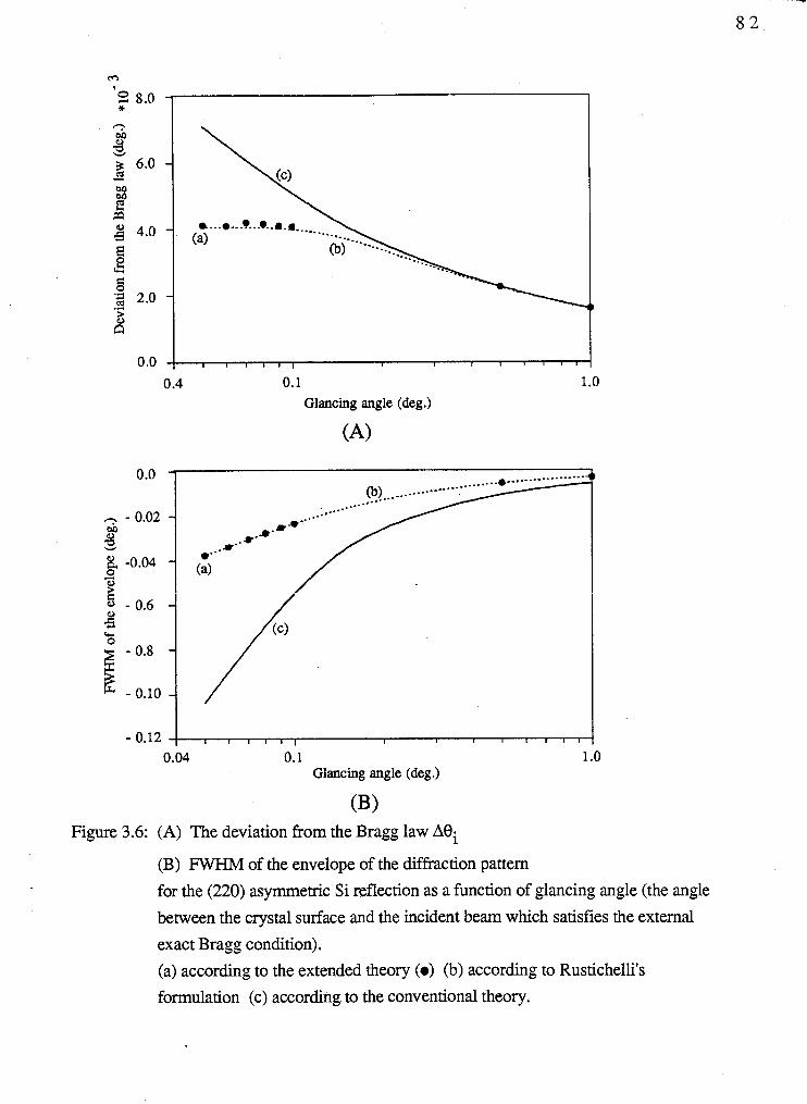
0.4 0.1 Glancing angle (deg.)

(A)

Figure 3.6: (A) The deviation from the Bragg law ABi

0.0 -

- 0.02 -

-0.04 -

- - - 0.6 0.10 0.8 - - -

- 0.12

(B) FWHM of the envelope of the diffraction pattern

for the (220) asymmetric Si reflection as a function of glancing angle (the angle

between the crystal surface and the incident beam which satisfies the external

. .................... .......... 0) ........-.....- ......... .... .-

m-*-'. *.a.

. * - a *" (a)

// I I I l l [ I I I I I l l 1

exact Bragg condition).

(a) according to the extended theory (e) (b) according to Rustichelli's

0.04 0.1 1 .O Glancing angle (deg.)

formulation (c) according to the conventional theory.

$cos2 (0 - a) - vo - 4 $sin2 BB cos2 a + 2 k, sin (8-a). 2 k, sin BB cos a = 0

$ - $ sin2 (8 - a) + 4 Gsin (9-a). sin eB cos a - v0 - 4 $sin2 eB cos2 a = O

2 vo sin2 (8 - a) - (4 sin $ cos a) sin (9-a) + 4 sin2 BB cos a c-- - 1 = 0 0

vo sin (9 - a) = 2 sin eB cos a +

sin (8 - a) = 2 sin eB cos a - vo - a-

Here we eliminate the solution with (+) sign by physical considerations. The approximate

misset angle is given by

where P1 = sin-' { 2 sin Bg cos a - 4- } . ko

(3.1 la)

The accurate value of misset angle corresponding to this border (~8);' can be calculated

using the fact that the surface normal becomes tangent to the ebranch of the dispersion

surface. Since only the tie points C, A and D are close to the Laue point in this case, one

could reduce the fourth order dispersion relation to the cubic equation of the form

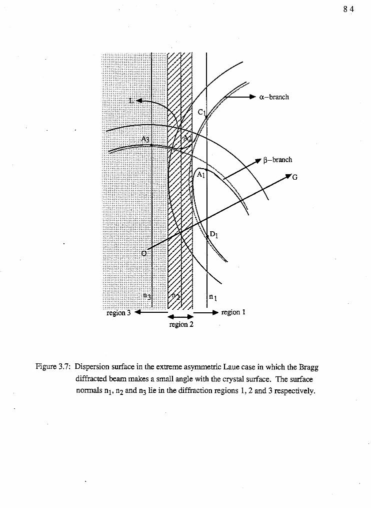
region 2

Figure 3.7: Dispersion surface in the extreme asymmetric Laue case in which the Bragg

diffracted beam makes a small angle with the crystal surface. The surface normals nl, n2 and n3 lie in the diffraction regions 1,2 and 3 respectively.

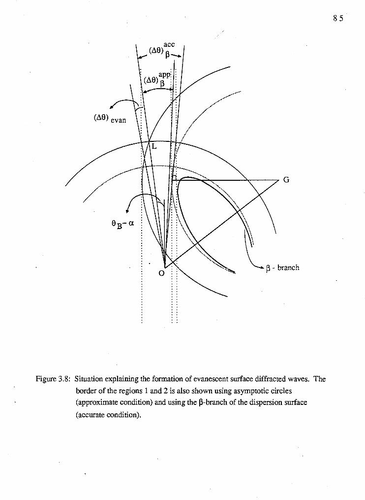
Figure 3.8: Situation explaining the formation of evanescent surface diffracted waves. The

border of the regions 1 and 2 is also shown using asymptotic circles (approximate condition) and using the P-branch of the dispersion surface

(accurate condition).

Mathematically the solutions of the above cubic equation are real and at least two have to be

equal at the rnisset angle of value ( A B ) ~ .

The border of the regions 2 and 3 can be calculated from the condition that the Bragg

diffracted and the specular diffracted waves become evanescent ( b Z and bmz become

imaginary quantities). This situation can be expressed mathematically as

(bx + Gx) 2 , (see Fig. 1.3)

i.e. G cos a - k, sin (8 - a ) 2 b

where 8 = BB + A8 and p2 = sin-' (2 sin eB cos a - 1).

Therefore, the rnisset angle corresponding to the border of the regions 2 and 3 (A@,, is

given by

(A@),, , ( ~ 0 ) ; ~ ~ and ( A B ) ~ are plotted against (eB + a ) in Fig. 3.9.

The amplitudes of the specular reflected wave and of the internal wave field

associated with the tie point B are negligible in this extreme asymmetric Laue case. We will

take them to be zero. However, the amplitude of the specular diffracted wave becomes

large. In this extreme case, the eqs. (3.4~) and (3.52) become equivalent (approximately)

to the eqs. (3.4a) and (3.5a) respectively (Same kind of argument given for the case 1 is

valid. The only difference is that the value of bz is small instead of koz in the case 1.

Therefore, one can assume that the values of ~ 2 ' ~ are approximately equal to &.).

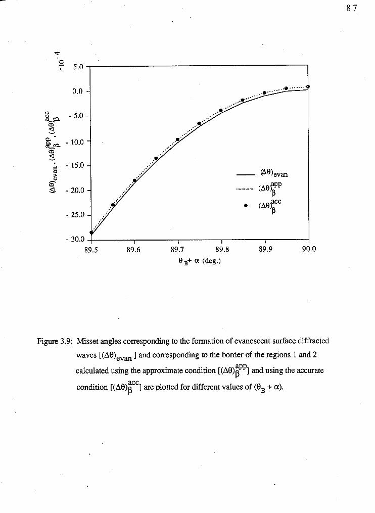
./ WJ) evan

89.5 89.6 89.7 89.8 89.9 90.0 0 ,+ a (deg.)

Figure 3.9: Misset angles corresponding to the formation of evanescent surface diffracted

waves [(AQeV, ] and corresponding to the border of the regions 1 and 2

calculated using the approximate condition [(A@ ] and using the accurate kPP condition [ ( A € ) ) ~ ~ ~ ] are plotted for different values of (BB + a). P

Using the equations (3.4a, b, d), (3.5a, b, d) and (3.6), we have calculated all the

unknown internal and external wave amplitudes. Note that the cubic equation which gives

the z components of the important internal wave vectors associated with the tie points C, A

and D (closer to the Laue point L) is of the form

in this extreme case. The intensities of the Bragg diffracted wave (at the lower surface of

the crystal) and of the specular diffracted wave (at the upper surface of the crystal) are

shown in Fig. 3.10(a) and (b) as a function of misset angle. The calculations were made

for the (220) Si reflection where the atomic planes make an angle a with the inward surface

normal such that (BB + a ) = 89.75'. In the region 3, the diffracted waves outside the

crystal are propagated along the crystal surfaces because the normal component of the wave

vectors are purely imaginary. Therefore the wave function of the Bragg diffracted wave at

the exit surface of the crystal is of the form odei ( i * h ) ei ( = Ode- ~ O Z . ei 'ox

'). Note that, the amplitude of this wave is equal to aGde- lQz . Therefore, the

intensities of the diffracted waves outside the crystal are exponentially attenuated in this

region as expected.

3.4.3 Extreme asymmetric Bragg case where the angle between the Bragg

diffracted beam and the crystal surface is small

The dispersion surface corresponding to this extreme case is shown in Fig. 3.11. In

Fig. 3.1 1, we distinguish five possible different angular ranges of diffraction. The surface

normals are denoted by nl, n2, n3, n4 and n5 in these five different regions. In the region

1, the surface normal nl intersects the dispersion surface in four real points; C1 and B1 lie

on the a-branch, A1 and Dl lie on the P-branch (note that the tie point B1 is far away from

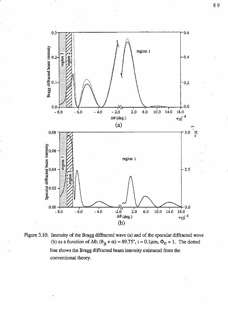
- 8.0 - 6.0 - 4.0 - 2.0 2.0 6.0 10.0 14.0 18.0

A0 (deg .) *16

region 1

Figure 3.10: Intensity of the Bragg diffracted wave (a) and of the specular diffracted wave (b) as a function of A0; (OB + a) = 89.75', t = 0.lp1-1, Qo = 1. The dotted

line shows the Bragg diffracted beam intensity estimated from the

conventional theory.

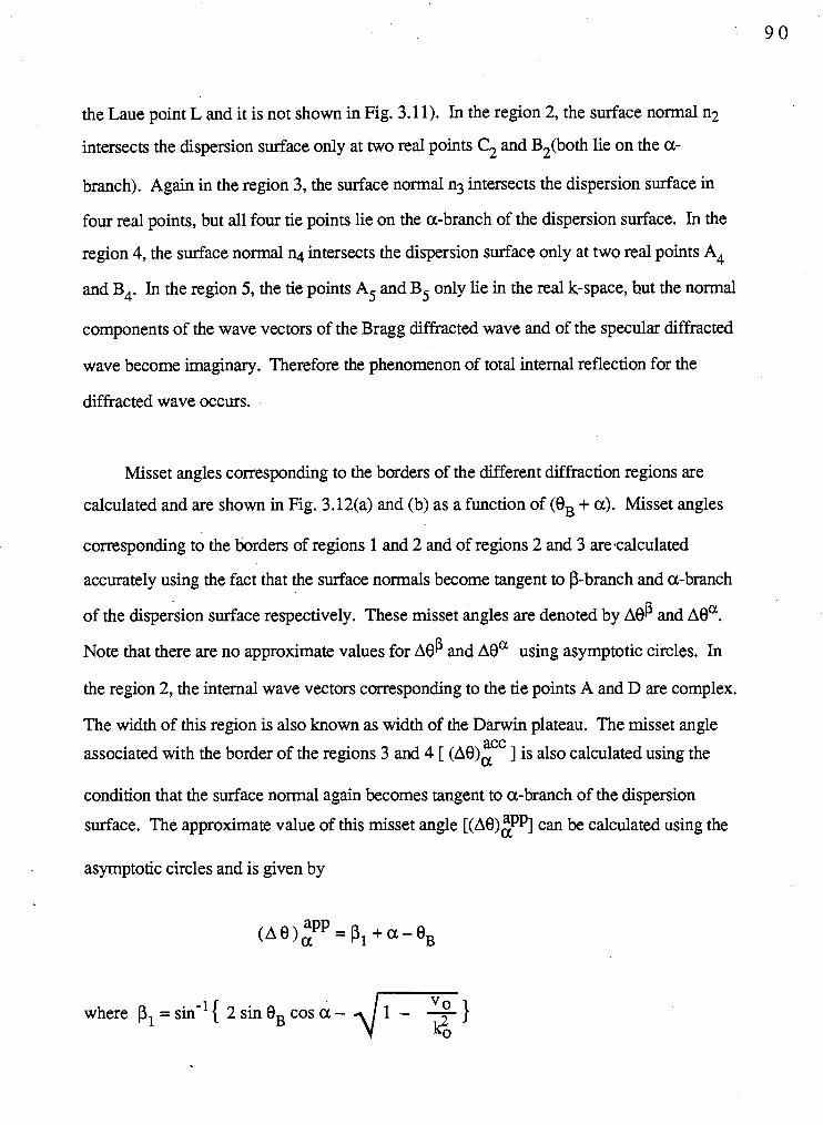
the Laue point L and it is not shown in Fig. 3.1 1). In the region 2, the surface normal n2

intersects the dispersion surface only at two real points C2 and B2(both lie on the a-

branch). Again in the region 3, the surface normal n3 intersects the dispersion surface in

four real points, but all four tie points lie on the a-branch of the dispersion surface. In the

region 4, the surface normal nq intersects the dispersion surface only at two real points A4

and B4. In the region 5, the tie points A5 and B5 only lie in the real k-space, hut the normal

components of the wave vectors of the Bragg diffracted wave and of the specular diffracted

wave become imaginary. Therefore the phenomenon of total internal reflection for the

diffracted wave occurs.

Misset angles corresponding to the borders of the different diffraction regions are

calculated and are shown in Fig. 3.12(a) and (b) as a function of (eB + a). Misset angles

corresponding to the borders of regions 1 and 2 and of regions 2 and 3 are.calculated

accurately using the fact that the surface normals become tangent to P-branch and a-branch

of the dispersion surface respectively. These misset angles are denoted by A@ and bea.

Note that there are no approximate values for A$ and ~ 0 " using asymptotic circles. In

the region 2, the internal wave vectors corresponding to the tie points A and D are complex.

The width of this region is also known as width of the Darwin plateau. The misset angle

associated with the border of the regions 3 and 4 [ ( A O ) ~ ] is also calculated using the

condition that the surface normal again becomes tangent to a-branch of the dispersion

surface. The approximate value of this misset angle [(Ae)tPp] can be calculated using the

asymptotic circles and is given by

vo when ~ l = s i n - 1 { 2 s i n 0 B c o s a - 41 -

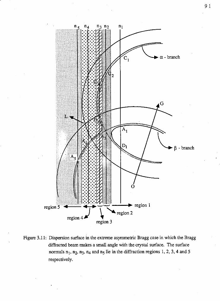
bra

region 4 region 3

p - branch

Figure 3.1 1: Dispersion surface in the extreme asymmetric Bragg case in which the Bragg

diffracted beam makes a small angle with the crystal surface. The surface normals nl, n2, n3, n4 and ng lie in the diffraction regions 1,2, 3 ,4 and 5

respectively.

The misset anglecorresponding to the border of the regions 4 and 5 is given by

eq. (3.13).

As we see from Fig. 3.11, the tie points C, A and D are closer to the Laue point L

and the internal wave fields corresponding to these tie points have to be taken into account.

The amplitudes of the fourth internal wave field associated with the tie point B which is far

away from the Laue point L, are extremely small and therefore this wave field may be

neglected. Furthermore the amplitude of the specular reflected can also be neglected in this

extreme case. Under these conditions, the eqs. (3.442) and (3%) obtained from the

boundary conditions, become equivalent (approximately) to eqs. (3.4a) and (3.5a) as for

the case 2. Note that the internal wave vectors associated with the tie points C, A and D

can be calculated from eq. (3.14). We have calculated the intensity of the diffracted waves

present at the upper and lower surfaces of the crystal using the boundary conditions and the

ratio of internal wave amplitudes. The results which covers all five different angular ranges

of diffraction are shown in Fig. 3.13(a) and (b). The intensity of the Bragg diffracted

wave at the entrance surface of the crystal is compared with the results obtained from the

conventional treatment. The calculations were made for the (220) Si reflection in which the

atomic planes make an angle a with the inward surface normal, satisfies the condition (eB

+ a ) = 90.25'. The intensity of the diffracted waves outside the crystal are exponentially

attenuated in the region 5 where the total internal reflection for the diffracted wave occurs.

The difference between the case 2 (section 3.4.2) and the case 3 (section 3.4.3) is the

number of possible different angular ranges of diffraction. In the case 2, there are only

three possible angular ranges of diffraction while there are five in the case 3. These two

cases are well separated by a situation where the surface normal cuts the a-branch of the

dispersion surface at four real points and three (which are closer to the Laue point L) out of

four tie,points have to coincide each other, i.e. the surface normal has to be tangent to the

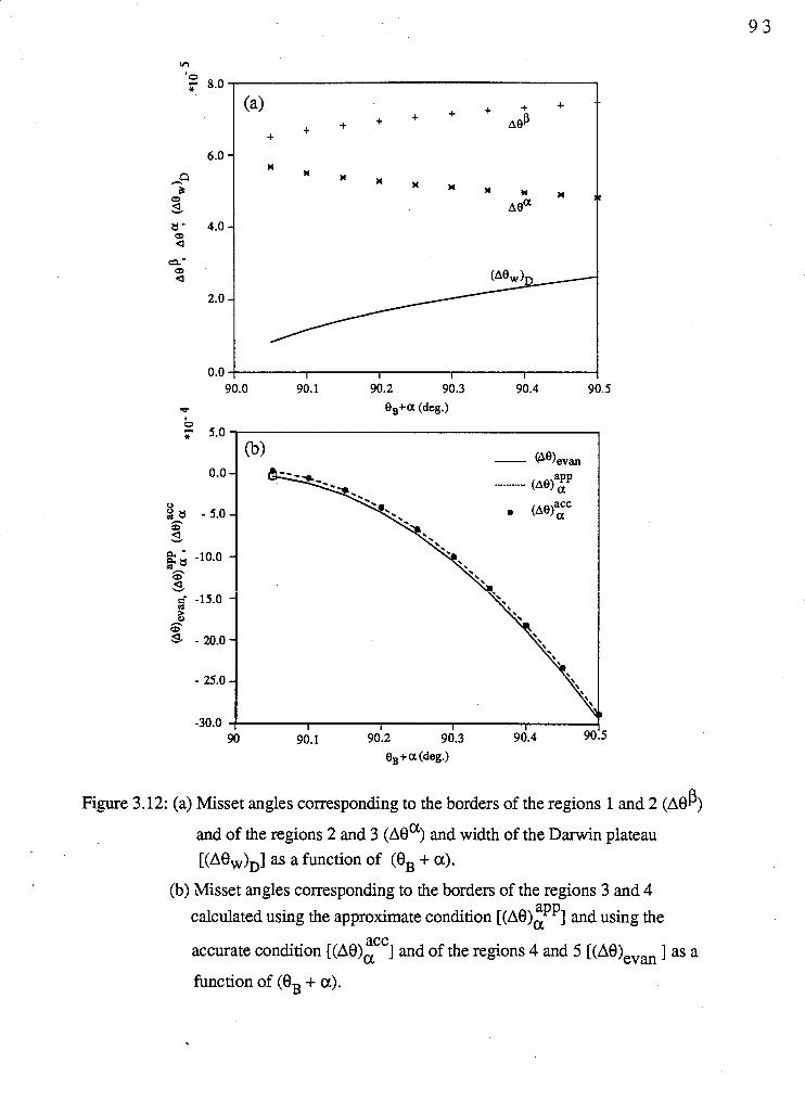
w 0,+a (deg.)

Figure 3.12: (a) Misset angles corresponding to the borders of the regions 1 and 2 (A84

and of the regions 2 and 3 ( ~ 8 ~ ) and width of the Darwin plateau [(~ie,)~] as a function of (eB + a).

(b) Misset angles corresponding to the borders of the regions 3 and 4 aPP calculated using the approximate condition ] and using the

accurate condition [ ( A B ) ~ ] and of the regions 4 and 5 [(A@,, ] as a

function of (eB + a).

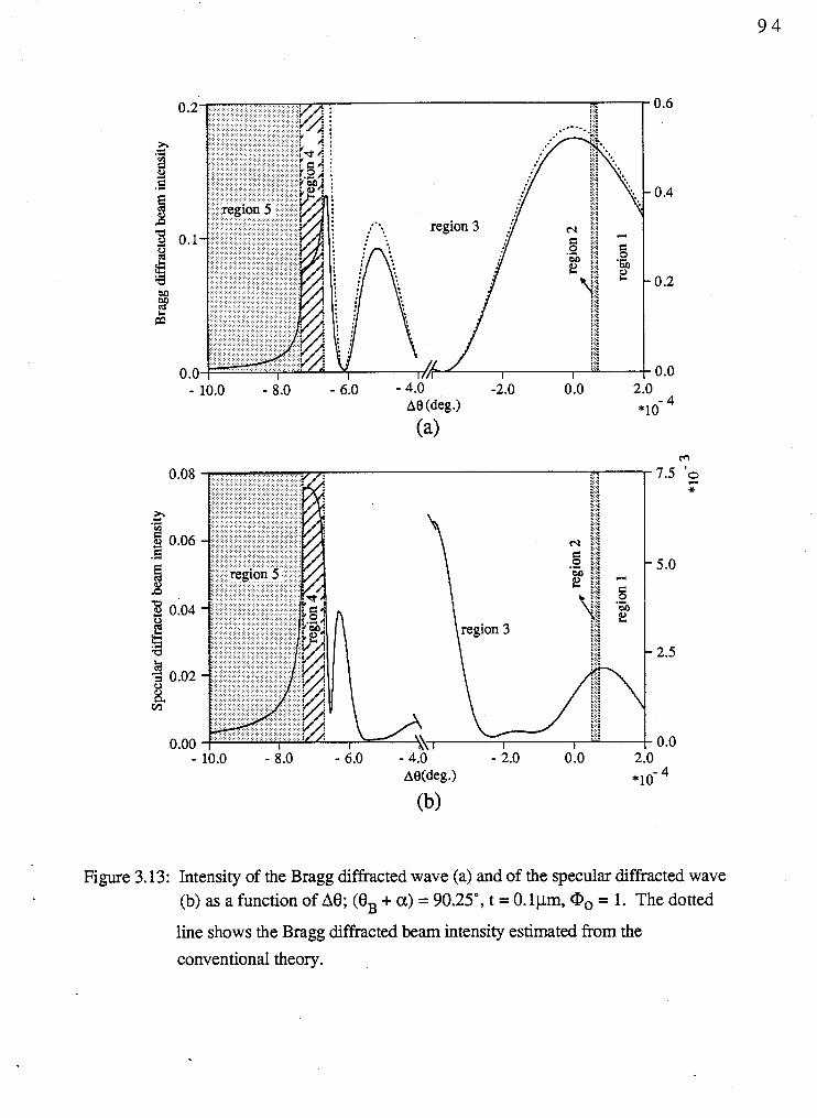
Figure 3.13: Intensity of the Bragg diffracted wave (a) and of the specula diffracted wave (b) as a function of A0; (Bg + a) = 90.25', t = 0. lpm, Q0 = 1. The dotted

line shows the Bragg diffracted beam intensity estimated from the

conventional theory.

a-branch of the dispersion surface at the inflection point of that branch. This situation can

be expressed mathematically by the condition that the solutions of the cubic equation (eq.

3.14) are real and also equal to each other. This situation occurs at a particular value of a

(*) for fixed k, and G or at a particular value of k, (*) for fixed values of a and G.

If we fixed the value of k, and G, we will get the extreme asymmetric cases like either case

2 or case 3 depending upon the value of a which is slightly less than or greater than e. Similarly, we will get the extreme asymmetric cases like either case 2 or case 3 depending

upon the value of k, which is slightly greater than or less than GB for fixed values of a

and G.

3.4.4 Extreme asymmetric Bragg case in which the incident beam makes a

small angle with the crystal surface

In this extreme case, there are two possible situations as shown as in Fig. 3.14(a) and

(b). In the first situation (Fig. 3.14(a)), we have distinguished four different regions of

diffraction. In the region 1, the surface normal nl cuts the dispersion surface in four real

tie points (A and D lie on the P-branch while C and B lie on the a-branch) and therefore

four wave fields associated with these tie points are excited inside the crystal. The surface

normal n2 cuts the dispersion surface in only two real tie points (both lie on the a-branch)

in the region 2. This is also known as Darwin plateau region. In the region 3, we have

again four real tie points, but now they are arranged on the a-branch of the dispersion

surface. Again we have only two real tie points in the region 4. This region is known as

the critical region.

The rnisset angles associated with the borders of the regions 1 and 2 ( A@ ) and the

regions 2 and 3 ( Aea ) are calculated using the fact that the surface normals become

tangent to P-branch and a-branch of the dispersion surface respectively. The width of the

Darwin'plateau (width of the region 2) is given by

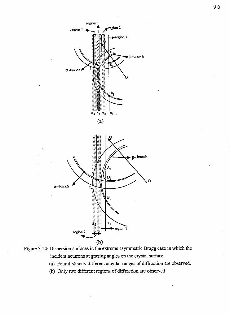
region 3

region 4 t / region

(b> Figure 3.14: Dispersion surfaces in the extreme asymmetric Bragg case in which the

incident neutrons at grazing angles on the crystal surface.

(a) Four distinctly different angular ranges of diffraction are observed.

(b) Only two different regions of diffraction are observed.

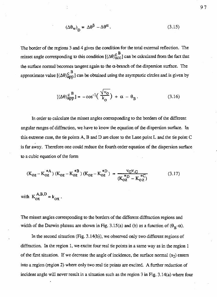
The border of the regions 3 and 4 gives the condition for the total external reflection. The B

misset angle corresponding to this condition [(Ae)CCc] can be calculated from the fact that

the surface normal becomes tangent again to the a-branch of the dispersion surface. The B

approximate value [ ( ~ e ) : ~ ~ ] can be obtained using the asymptotic circles and is given by

In order to calculate the misset angles corresponding to the borders of the different

angular ranges of diffraction, we have to know the equation of the dispersion surface. In

this extreme case, the tie points A, B and D are close to the Laue point L and the tie point C

is far away. Therefore one could reduce the fourth order equation of the dispersion surface

to a cubic equation of the form

A,BD - with K,, - kox .

The misset angles corresponding to the borders of the different diffraction regions and

width of the Danvin plateau are shown in Fig. 3.15(a) and (b) as a function of (BB-a).

In the second situation (Fig. 3.14(b)), we observed only two different regions of

diffraction. In the region 1, we excite four real tie points in a same way as in the region 1

of the first situation. If we decrease the angle of incidence, the surface normal (n2) enters

into a region (region 2) where only two real tie points are excited. A further reduction of

incident angle will never result in a situation such as the region 3 in Fig. 3.14(a) where four

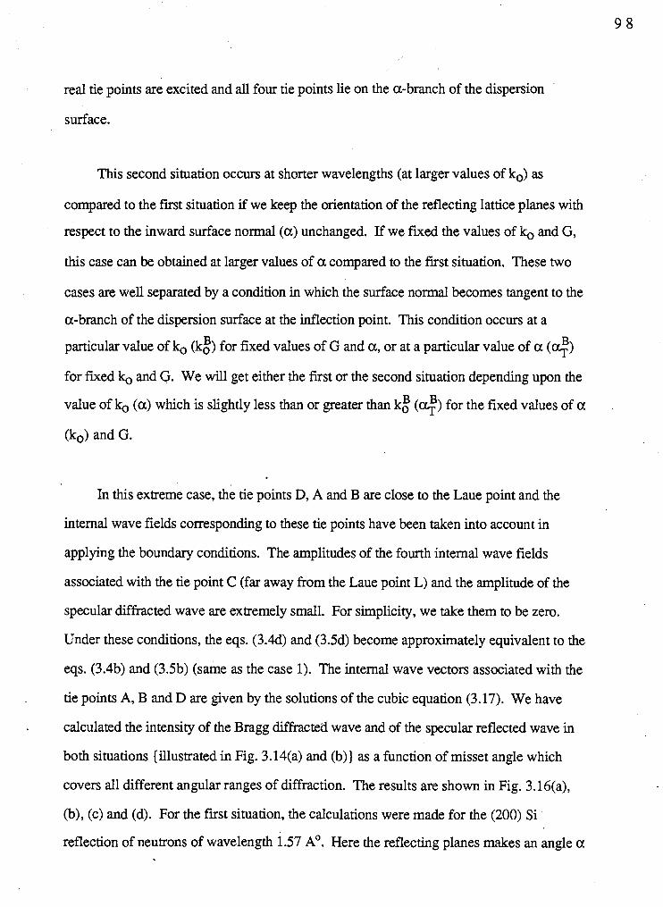
real tie points are excited and all four tie points lie on the a-branch of the dispersion

surface.

This second situation occurs at shorter wavelengths (at larger values of ko) as

compared to the fust situation if we keep the orientation of the reflecting lattice planes with

respect to the inward surface normal (a) unchanged. If we fixed the values of k, and G,

this case can be obtained at larger values of a compared to the first situation. These two

cases are well separated by a condition in which the surface normal becomes tangent to the

a-branch of the dispersion surface at the inflection point. This condition occurs at a

particular value of k, (k:) for fixed values of G and a, or at a particular value of a (G) for fixed k, and G. We will get either the first or the second situation depending upon the

value of k, (a) which is slightly less than or greater than k: (4) for the fixed values of a

(ko) and G.

In this extreme case, the tie points D, A and B are close to the Laue point and the

internal wave fields corresponding to these tie points have been taken into account in

applying the boundary conditions. The amplitudes of the fourth internal wave fields

associated with the tie point C (far away from the Laue point L) and the amplitude of the

specular diffracted wave are extremely small. For simplicity, we take them to be zero.

Under these conditions, the eqs. (3.44 and (3.5d) become approximately equivalent to the

eqs. (3.4b) and (3.5b) (same as the case 1). The internal wave vectors associated with the

tie points A, B and D are given by the solutions of the cubic equation (3.17). We have

. calculated the intensity of the Bragg diffracted wave and of the specular reflected wave in

both situations {illustrated in Fig. 3.14(a) and (b)) as a function of misset angle which

covers all different angular ranges of diffraction. The results are shown in Fig. 3.16(a),

(b), (c) and (d). For the first situation, the calculations were made for the (200) Si

reflection of neutrons of wavelength 1.57 A'. Here the reflecting planes makes an angle a

Figure 3.15: (a) Misset angles corresponding to the borders of the regions 1 and 2

and of the regions 2 and 3 ( ~ 8 ~ ) and width of the Darwin plateau as a function of (eB - a).

(b) Misset angle corresponding to the border of the regions 3 and 4 calculated

using the approximate condition [ ( ~ 0 ) ~ ~ 1, the accurate condition aPP

4 [ ( ~ e ) ~ ~ ~ ~ ] and the difference ( (A0gPp - (AO)&~ ) (x 10 ) as a

function of (eB - a).

The calculations were made for a fixed value of eB and by changing the value

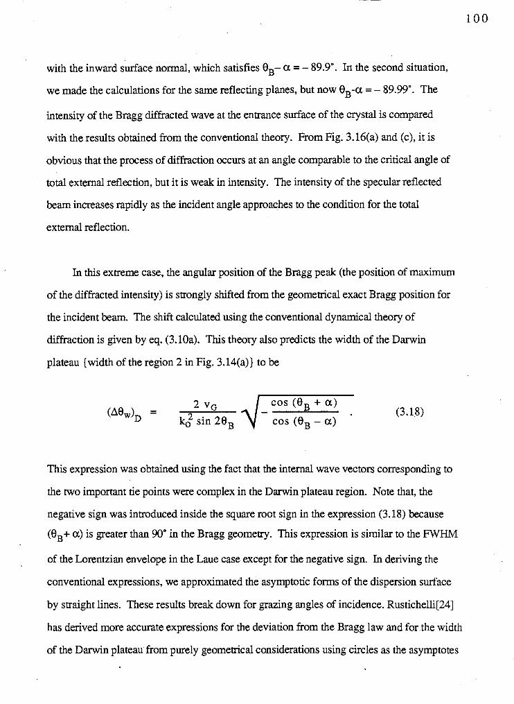
with the inward surface normal, which satisfies eB- a = - 89.9". In the second situation,

we made the calculations for the same reflecting planes, but now eB-a = - 89.99". The

intensity of the Bragg diffracted wave at the entrance surface of the crystal is compared

with the results obtained from the conventional theory. From Fig. 3.16(a) and (c), it is

obvious that the process of diffraction occurs at an angle comparable to the critical angle of

total external reflection, but it is weak in intensity. The intensity of the specular reflected

beam increases rapidly as the incident angle approaches to the condition for the total

external reflection.

In this extreme case, the angular position of the Bragg peak (the position of maximum

of the diffracted intensity) is strongly shifted from the geometrical exact Bragg position for

the incident beam. The shift calculated using the conventional dynamical theory of

diffraction is given by eq. (3.10a). This theory also predicts the width of the Darwin

plateau {width of the region 2 in Fig. 3.14(a)) to be

- cos (eB + a ) (W, -

cos (eB - a )

This expression was obtained using the fact that the internal wave vectors corresponding to

the two important tie points were complex in the Darwin plateau region. Note that, the

negative sign was introduced inside the square root sign in the expression (3.18) because

(eB+ a ) is greater than 90" in the Bragg geometry. This expression is similar to the FWHM

of the Lorentzian envelope in the Laue case except for the negative sign. In deriving the

conventional expressions, we approximated the asymptotic forms of the dispersion surface

by straight lines. These results break down for grazing angles of incidence. Rustichelli[24]

has derived more accurate expressions for the deviation from the Bragg law and for the width

of the Darwin plateau from purely geometrical considerations using circles as the asymptotes

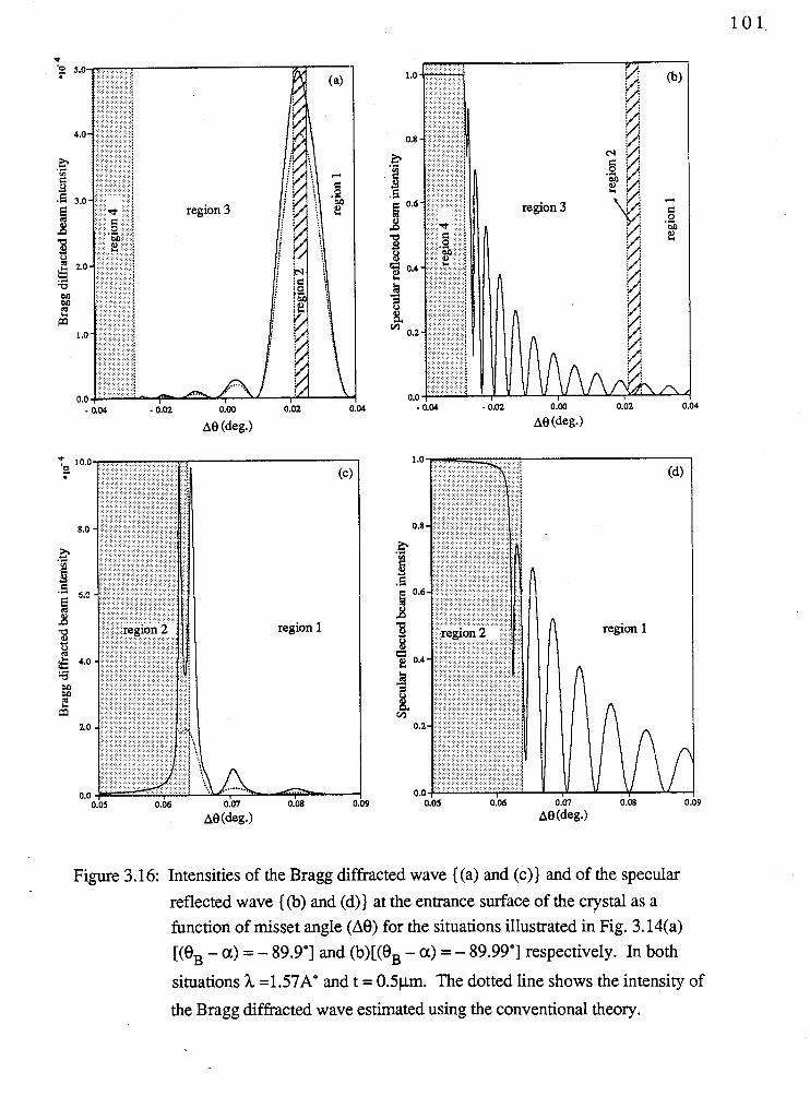
Figure 3.16: Intensities of the Bragg diffracted wave {(a) and (c)) and of the specular

reflected wave {(b) and (d)) at the entrance surface of the crystal as a

function of misset angle (A@) for the situations illustrated in Fig. 3.14(a) [($ - a ) = - 89.9'1 and (b)[(OB - a ) = - 89.99'1 respectively. In both

situations h =1.57A0 and t = 0.5ym. The dotted line shows the intensity of

the Bragg diffracted wave estimated using the conventional theory.

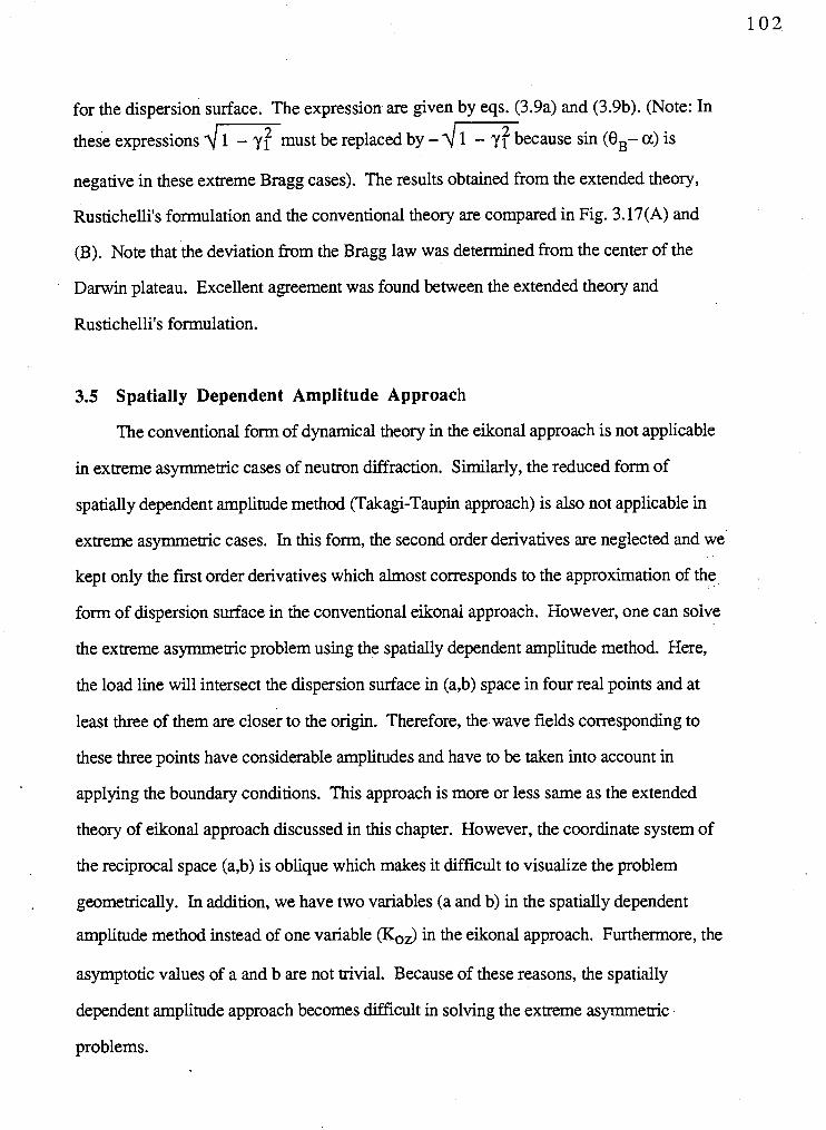
for the dispersion surface. The expression are given by eqs. (3.9a) and (3.9b). (Note: In

these expressions 4-must be replaced by - . I n b e c a u s e sin (0,- a) is

negative in these extreme Bragg cases). The results obtained from the extended theory,

Rustichelli's formulation and the conventional theory are compared in Fig. 3.17(A) and

(B). Note that the deviation from the Bragg law was determined from the center of the

Darwin plateau. Excellent agreement was found between the extended theory and

Rustic helli's formulation.

3.5 Spatially Dependent Amplitude Approach

The conventional form of dynarnical theory in the eikonal approach is not applicable

in extreme asymmetric cases of neutron diffraction. Similarly, the reduced form of

spatially dependent amplitude method (Takagi-Taupin approach) is also not applicable in

extreme asymmetric cases. In this form, the second order derivatives are neglected and we'

kept only the first order derivatives which almost corresponds to the approximation of the

form of dispersion surface in the conventional eiiconai approach. However, one can soive

the extreme asymmetric problem using the spatially dependent amplitude method. Here,

the load line will intersect the dispersion surface in (a,b) space in four real points and at

least three of them are closer to the origin. Therefore, the. wave fields corresponding to

these three points have considerable amplitudes and have to be taken into account in

applying the boundary conditions. This approach is more or less same as the extended

theory of eikonal approach discussed in this chapter. However, the coordinate system of

the reciprocal space (a,b) is oblique which makes it difficult to visualize the problem

geometrically. In addition, we have two variables (a and b) in the spatially dependent

amplitude method instead of one variable (I&) in the eikonal approach. Furthermore, the

asymptotic values of a and b are not trivial. Because of these reasons, the spatially

dependent amplitude approach becomes difficult in solving the extreme asymmetric

problems.

Grazing angle (deg.)

(A)

0.1 Grazing angle (deg.)

(B)

Figure 3.17: (A) The deviation from the Bragg law Aei

(B) Width of the Darwin plateau

for (220) asymmetric Si reflection as a function of glazing angle (the angle

between the crystal surface and the incident beam which satisfies the external

exact Bragg condition).

(a) according to the extended theory (e) (b) according to Rustichelli's

fornulation (c) according to the conventional theory.

CHAPTER 4

DYNAMICAL THEORY OF DIFFRACTION FOR BENT CRYSTALS

4.1 Introduction

In the last three decades, diffraction phenomena in deformed crystals have been

studied both theoretically and experimentally. The dynamical theory of x-ray diffraction

from a bent crystal was first developed by Penning and Polder (1961)[25] and Kato

(1964)[26]. They used the eikonal approximation and explained some experimental

results. However, because of the strong restrictions associated with the conditions for the

applicability of the eikonal approximation, this theory does not give the correct description

of X-ray diffraction in strongly distorted crystal regions, nor near the edges of the

Borrmann triangle.

A second approach of dynamicd theory of diffraction for a distorted crystal was

developed by Takagi (1962,1969)[8] and Taupin [9]. This theory was developkd purely

based on wave-optical phenomena So far, the Takagi-Taupin type equations have been

solved exactly only for the case of a crystal with a uniform strain gradient [I 1 and

references therein]. The analytical solutions of these equations are expressed in terms of

confluent hypergeometric functions. The mathematical treatment of these functions is very

complicated. However, the physical analysis of this solution is absolutely necessary to

give an adequate explanation for the diffraction phenomenon in a homogeneously bent

crystal. The wave field, which was obtained using the asymptotic forms of the confluent

. hypergeometric function, tends to results of kinematical theory as the strain gradient

increases, and tends to the solution of the eikonal theory with decreasing strain gradient.

Therefore, this approach can be used to explain the diffraction phenomenon from a crystal

with a wide range of distortion.

We have modified the theory of x-ray diffraction from a homogeneously bent crystal

based on the Takagi-Taupin equations to treat the neutron case. The details are given in this

chapter. The complication of the mathematical treatment of confluent hypergeometric

functions have been such that little use has been made in this approach by workers in this

field. We have eliminated the mathematical obscurity by expressing the confluent

hypergeometric function in terms of Chebyshev polynomials. This makes it possible to

study the neutron diffraction phenomena from a homogeneously bent crystal numerically.

We have chosen the type of homogeneous bending which was elaborated by Penning and

Polder [25] as an example. Here we study the diffraction pattern (rocking curves) for

different amplitudes of the strain gradient, integrated intensity as a function of curvature of

bending, and dynamical thickness oscillations of integrated intensity in the Laue diffraction

geometry. The results, computed numerically, are discussed in this chapter.

Elasticity theory adds more complications if theory is to be compared with

experiments. The diffraction theory has been well established only in the case of a uniform

strain gradient. In most experimental arrangements which were intended to produce

uniform strain gradients, the strain gradient varies with the position. Yet, most of the

researchers in this field have assumed the simplest form of displacement field which

corresponds to the uniform strain gradient. The appropriate displacement field

corresponding to the experimental arrangement can be found only by using elasticity

theory. We have considered the bending of crystals by loading along two lines at each of

two edges as an example. By using the conventional bending theory of thin crystal plates,

. we have found that higher order (> second order) terms of the coordinates of the position

are necessary in order to specify the appropriate displacement field. These results indicate

that the local radii of curvature vary position to position and even change sign. Either they

can be calculated from the mid-surface displacements or can be measured experimentally.

In diffraction theory, when we calculate the intensity of the diffracted beam at an arbitrary

point, only the strain field in the inverse Bomann triangle associated with that point

matters. The far strain fields won't come into the problem. The width of Borrmann

triangles are very small compared to the length and width of crystal plates which we used in

our experiments. Therefore one can assume that the strain gradient in any Bonmann

triangle is uniform and they are determined by local radii of curvature. Now one can apply

the solutions of diffraction theory as developed for the case of a uniform strain gradient to

calculate the intensity of the diffracted beam at any point on the exit surface of the crystal.

These remarks are discussed in detail in this chapter.

In most of our experiments we have exceeded the limits in which the conventional

theory of bending can be applied, that is the displacements of the mid-surface become

greater than the thickness of the crystal. In-plane forces (as a result of large curvature),

which are neglected in the conventional bending theory, now have to be taken into account.

This result in a pair of coupled non linear fourth order differential equations. There are no

known non trivial solutions of these differential equations.

4 .2 Solution to a uniform strain gradient problem using Takagi-Taupin

equations

In the perfect crystal, the reduced neutron -nuclear interaction potential can be written

as

-9 Here we assume that the incident wave vector kois oriented very close to the exact Bragg

condition for a particular reciprocal lamce vector -d. Therefore, the Fourier components of

the potential corresponding to the other reciprocal lamce vectors are neglected.

~etl?(T') be the displacement of the atom at ? in a slightly distorted crystal and 6 be the position vector of the atom before the distortion which is now displaced to? during

distortion. Thus the relation between T' and i$ is given by

++ Note that, u ( r ) is a continuous function. If the distortion is slight (i.e. as long as the

atoms within a single unit cell can be regarded as being uniformly displaced), the value of

v(? ) in the distorted crystal can be mapped to the value of the reduced potential in the

perfect crystal at the corresponding position s, i.e.

In these equations, d is the reciprocal lamce vector for the undistorted crystal. In this

approximation, the changes in Fourier coefficients and d on bending are neglected. The

spatial frequency of the potential is modulated due to strain gradients. The effect of this

variation in the potential on the internal wave function will be modeled using a single spatial

frequency with amplitude modulation. Therefore, the wave function in a distorted crystal

can be expressed by a sum of modulated waves

Under the same assumption as mentioned above, we anticipate the wave function to be of

the form

where

With the assumption that the amplitudes yo(?) and lG(?) are slowly varying functions of

position, the terms v2y0(?) and v2yG(?) are small compared with terms proportional to

lo (? ) and yG(?) or their first derivatives and can be neglected. By substituting the

reduced periodic potential given by eq. (4.3) and the above form of the wave function {eq.

(4.4)) into the Schrijdinger equation for the neutron {eq. (1.13)) and using the oblique

coordinate system described in chapter 1, we will get the following coupled differential

equations:

where K is the magnitude of the internal wave vector % and has the value -,/Go. These above equations (4.5a) and (4.5b) are the Takagi-Taupin type equations for a

++' distorted crystal. These expressions are the same as the eqs. (1.41a & b) if u ( r ) = 0.

In the general case of a crystal with a uniform strain gradient, the function 8.3 is of

the form

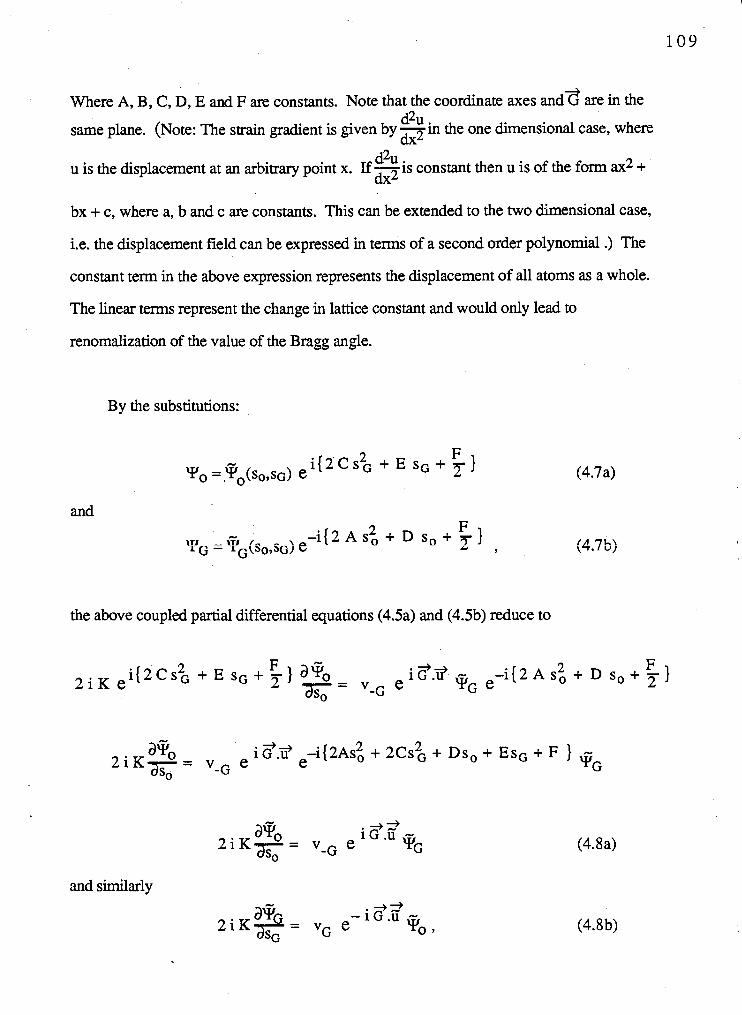
Where A, B, C, D, E and F are constants. Note that the coordinate axes a n d 2 are in the d2u

same plane. (Note: The strain gradient is given by -in the one dimensional case, where dx2

d2u u is the displacement at an arbitrary point x. If -is constant then u is of the form ax2 +

dx2

bx + c, where a, b and c are constants. This can be extended to the two dimensional case,

i.e. the displacement field can be expressed in terms of a second order polynomial .) The

constant term in the above expression represents the displacement of all atoms as a whole.

The linear terms represent the change in lattice constant and would only lead to

renomalization of the value of the Bragg angle.

By the substitutions:

and

the above coupled partial differential equations (4.5a) and (4.5b) reduce to

and similarly

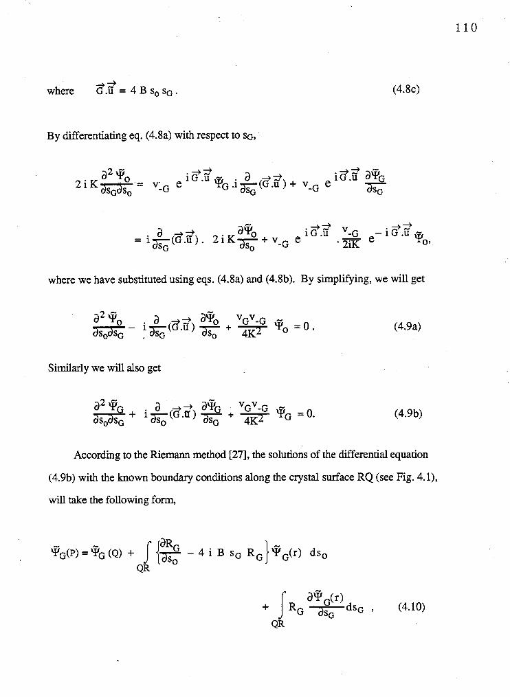
where 3.2 = 4 B so so .

By differentiating eq. (4.8a) with respect to Q,

where we have substituted using eqs. (4.8a) and (4.8b). By simplifying, we will get

Similarly we will also get

According to the Riemann method [27], the solutions of the differential equation

(4.9b) with the known boundary conditions along the crystal surface RQ (see Fig. 4. I),

will take the following form,

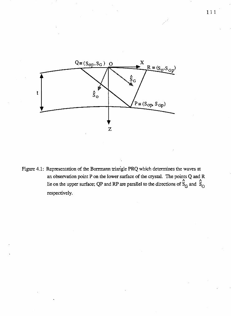
Figwe 4.1: Represent~tbn d the 130m=n trh.igb PRO whi& detdnes he wwes zt

an observation point P on the lower surface of the crystal. The points Q and R A A

lie on the upper surface; QP and RP are parallel to the directions of SG and So

respectively.

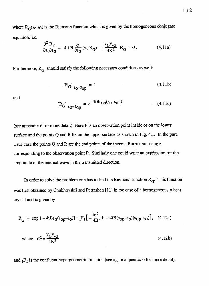
where R G ( s O , ~ ~ ) is the Riemann function which is given by the homogeneous conjugate

equation, i.e.

Furthermore, RG should satisfy the following necessary conditions as well:

and

(4.1 la)

(see appendix 6 for more detail) Here P is an observation point inside or on the lower

surface and the points Q and R lie on the upper surface as shown in Fig. 4.1. In the pure

Laue case the points Q and R are the end points of the inverse Borrmann triangle

corresponding to the observation point P. Similarly one could write an expression for the

amplitude of the internal wave in the transmitted direction.

In order to solve the problem one has to find the Riemann function RG. This function

was first obtained by Chukhovskii and Petrashen [I 11 in the case of a homogeneously bent

crystal and is given by

V ~ V - ~ where 02= - 4 ~ 2

(4.12b)

and is the confluent hypergeometric function (see again appendix 6 for more detail).

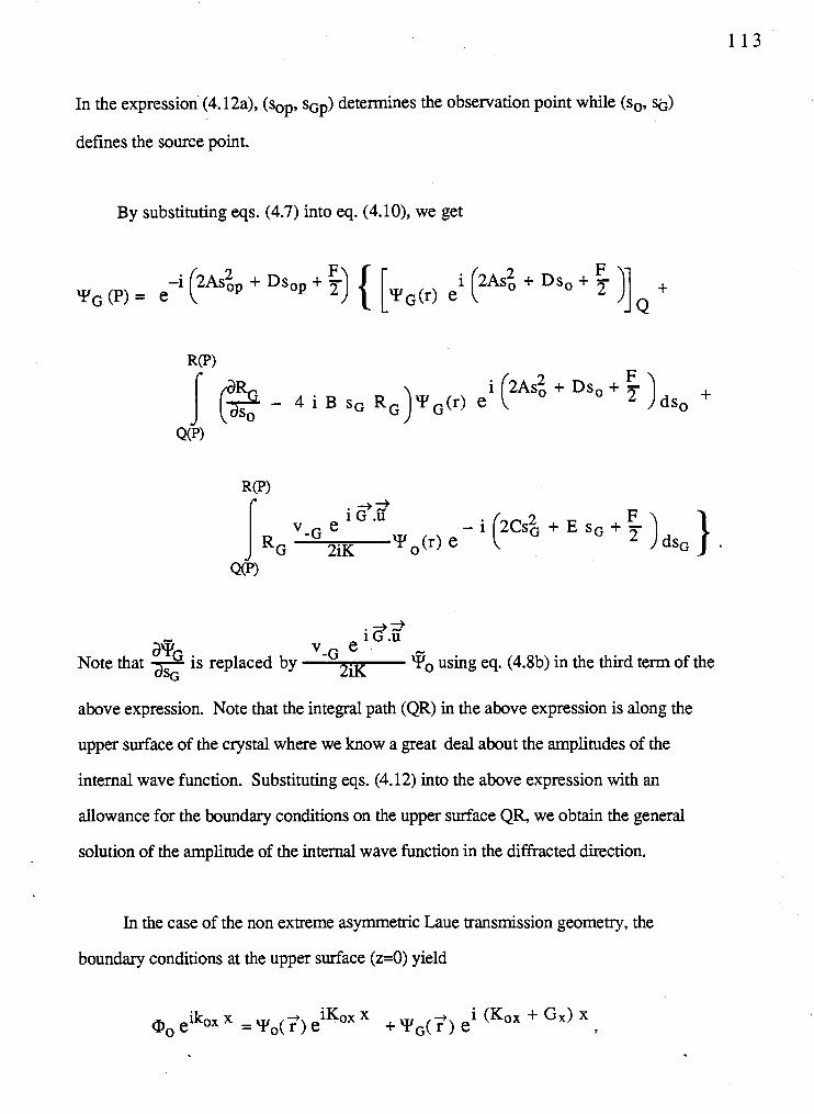
In the expression (4.12a), (sop, sop) determines the observation point while (so, sij)

defines the source point.

By substituting eqs. (4.7) into eq. (4.10), we get

, ,

+ Ds, + F ) dso +

V-G e i 3.2

aqG Note that is replaced by 2iK go using eq. (4.8b) in the third term of the

SG

above expression. Note that the integral path (QR) in the above expression is along the

upper surface of the crystal where we know a great deal about the amplitudes of the

internal wave function. Substituting eqs. (4.12) into the above expression with an

allowance for the boundary conditions on the upper surface QR, we obtain the general

solution of the amplitude of the internal wave function in the diffracted direction.

In the case of the non extreme asymmetric Laue transmission geometry, the

boundary conditions at the upper surface (z=O) yield

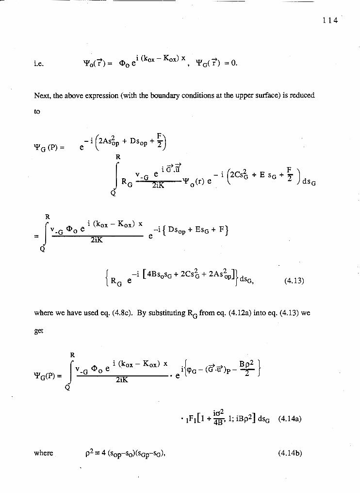
Next, the above expression (with the boundary conditions at the upper surface) is reduced

to

where we have used eq. (4.8~). By substituting RG from eq. (4.12a) into eq. (4.13) we

get

where

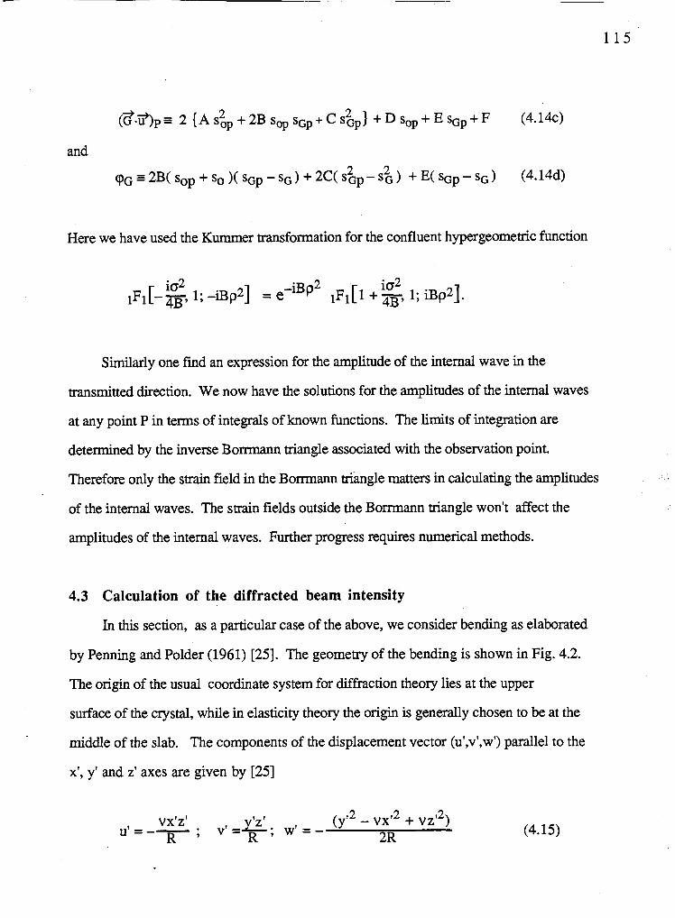
Here we have used the Kummer transformation for the confluent hypergeometric function

Similarly one find an expression for the amplitude of the internal wave in the

transmitted direction. We now have the solutions for the amplitudes of the internal waves

at any point P in terms of integrals of known functions. The limits of integration are

determined by the inverse Bomnann triangle associated with the observation point.

Therefore only the strain field in the Bomann triangle matters in calculating the amplitudes

of the internal waves. The strain fields outside the Borrmann triangle won't affect the

amplitudes of the internal waves. Further progress requires numerical methods.

4.3 Calculation of the diffracted beam intensity

In this section, as a particular case of the above, we consider bending as elaborated

by Penning and Polder (1961) [25]. The geometry of the bending is shown in Fig. 4.2.

The origin of the usual coordinate system for diffraction theory lies at the upper

surface of the crystal, while in elasticity theory the origin is generally chosen to be at the

middle of the slab. The components of the displacement vector (ul,v',w') parallel to the

x', y' and z' axes are given by [25]

2 2 vx'z' Y'Z' . (y'2 - vx' + vz' ) U' = -- ' R 9 v ' - R , w t = -

2R

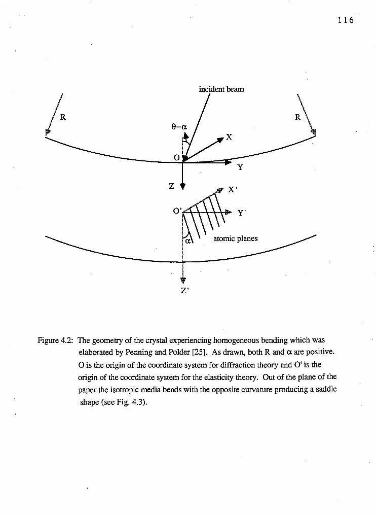
incident beam

z '

Figure 4.2: The geometry of the crystal experiencing homogeneous bending which was elaborated by Penning and Polder [25]. As drawn, both R and a are positive.

0 is the origin of the coordinate system for diffraction theory and 0' is the

origin of the coordinate system for the elasticity theory. Out of the plane of the

paper the isotropic media bends with the opposite curvature producing a saddle

shape (see Fig. 4.3).

1 1 7

respectively, where R is the radius of curvature and v is Poisson's ratio. Note that the local

radii of curvature of the mid-surface in planes parallel to yz and xz, R and - R/v, are

constant and independent of position. These results are obtained for a prismatic beam

which is bent in one of its principal planes by two equal and opposite couples [28]. In

deriving these displacement components, they ignore the fact that the crystal is a crystal and

treat the crystalline media as an isotropic medium with Poisson's ratio V. We need the

components of the displacement vector (u,v,w) parallel to the x, y and z axes of the

coordinate system with origin at 0 in order to calculate the coefficients A, B, C, D, E and

F. These components are given by

Note that the relations between the two coordinate systems &e x'=x, y'=y and

z'= 1 z - I) , where t is the thickness of the crystal. The mid-surface displacement 2 '2

calculated using the above equation (4.16) is saddle shaped as shown in Fig 4.3.

We consider the reflection corresponding to the lattice planes whose scattering vector

is in the xz plane at y = 0, where the bending takes place as the result of an enforced bend

in the yz plane. The reciprocal lattice vector -d associated with these reflecting planes make

an angle a with the crystal surface. Then,

vx{z - $1 [ - v x 2 + v { z -;I2] =-Gcos a R + G sin a 2R (4.17)

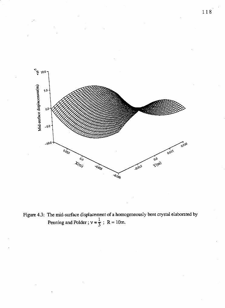
Figure 4.3: The mid-surface displacement of a homogeneously bent crystal elaborated by 1

Penning and Polder ; v = ; R = 10m.

By comparing the eq. (4.17) with the eq. (4.6), the coefficients A, B, C, D, E and F can be

determined. They are given by the following relations (see appendix 7):

* 1 a2 + A =--(&I ) = v G sin ( 2 8 ~ - a ) 4 as$ 4 R

a2 ( 3 . 3 ) = - v G sin a B = ~ w 4 R

1 a2 c=-- (&?) =- v G sin (28; + a ) 4 as$ 4 R

* D = constant term of -J- (G .U ) = -

K O ++ I v G t sin OB 2 R

* v G t sin eB

E = constant term of 2 R

V G t 2 s i n a F = constant term of ( 3 . 2 ) = 8 R

In order to calculate the internal wave amplitudes, one should know how to handle

the confluent hypergeometric function. The mathematical treatment of this function is very

complicated. However, one can expand the confluent hypergeometric function in an

ascending series of Chebyshev polynomials [28], i.e.

* where Tn (x I 5) = Tn(2x - 1) = cos {n cos -1 (2x - 1)) (4.19b)

is the shifted Chebyshev polynomials of the first kind and w is the preselected scale factor

L such that 0 < i 1.

The coefficients of the above expansion Cn(w) satisfy the following recurrence formula.

where@= 1 a n d ~ ~ = 2 f o r n > O .

The coefficients Cn(w)'s can be found by using the above recursion formula {eq. (4.20))

in the backward direction, together with the following normalization relation

This means if we work with (n+l) terms, we take Cn+2 = 0, Cn+3 = 0 and Cn+l = C

(constant) and calculate Cn using the above recursion relation {eq. (4.20)) and finally 00

scale the coefficients dividing by (- 1)" Cn(w). n=O

Now we can calculate the diffracted wave amplitude (the approximate value depends

on the value of n) numerically using the expansion of confluent hypergeometric function in

terms of Chebyshev polynomials. The diffraction profiles are calculated as a function of

rnisset angle for different values of curvature with v = $. The calculations are made for the

(400) Si reflection ((1 11) cut crystal) in which the crystal surface is parallel to ( 4 2 ).

Because of the Pendelliisung fringes in the Laue geometry, the diffraction profiles depend

strongly on the thickness of the crystal. However, we fixed the crystal thickness ( 75 pm)

to study the dependence of the diffraction profile on the curvature of the bending. The

results are shown in Fig 4.4. The rocking curves retain the box-like shape characteristics,

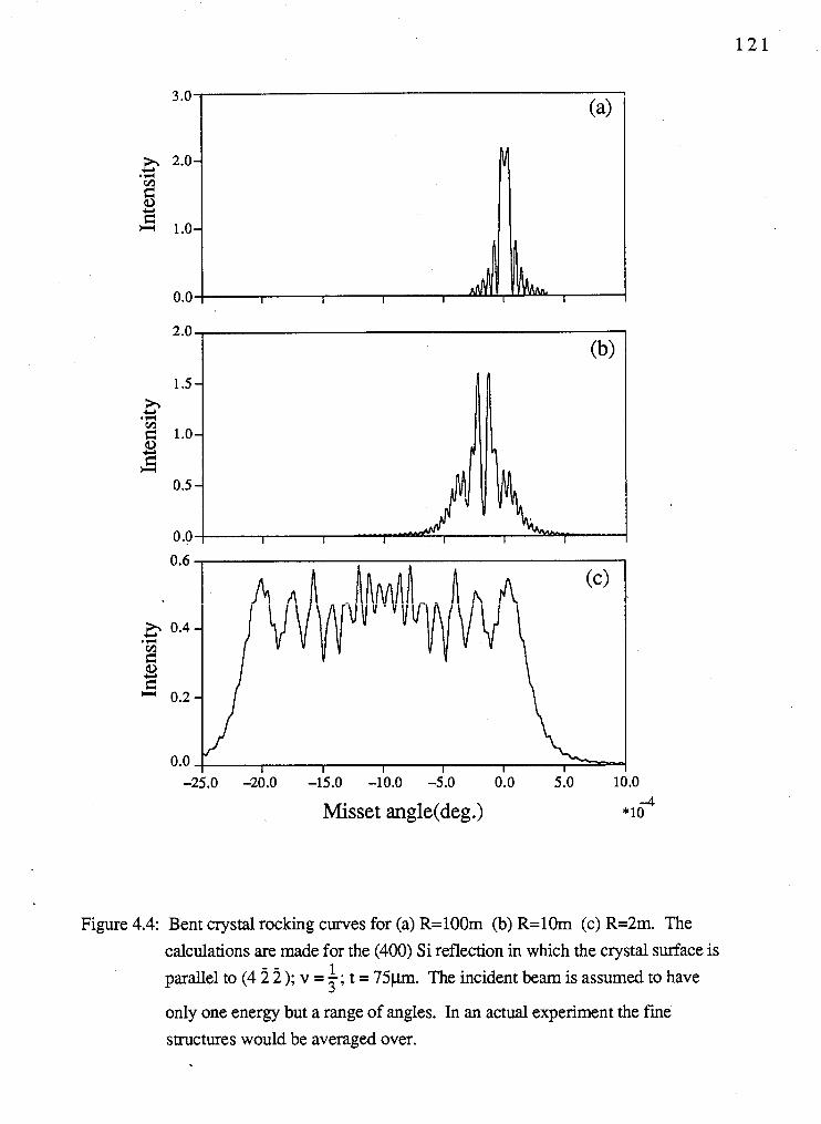
Misset angle(deg.)

Figure 4.4: Bent crystal rocking curves for (a) R=100m (b) R=lOm (c) R=2m. The

calculations are made for the (400) Si reflection in which the crystal surface is 1 parallel to (4 3 3 ); v = 5 ; t = 7 5 p . The incident beam is assumed to have

only one energy but a range of angles. In an actual experiment the fine

structures would be averaged over.

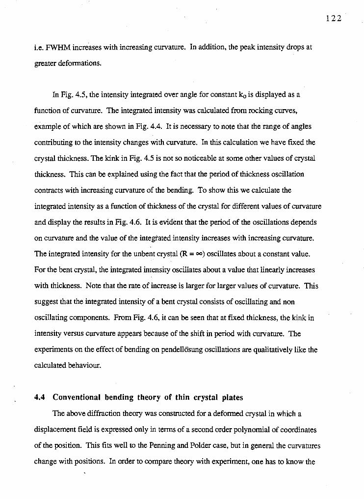
i.e. FWHM increases with increasing curvature. In addition, the peak intensity drops at

greater deformations.

In Fig. 4.5, the intensity integrated over angle for constant ko is displayed as a

function of curvature. The integrated intensity was calculated from rocking curves,

example of which are shown in Fig. 4.4. It is necessary to note that the range of angles

contributing to the intensity changes with curvature. In this calculation we have futed the

crystal thickness. The kink in Fig. 4.5 is not so noticeable at some other values of crystal

thickness. This can be explained using the fact that the period of thickness oscillation

contracts with increasing curvature of the bending. To show this we calculate the

integrated intensity as a function of thickness of the crystal for different values of curvature

and display the results in Fig. 4.6. It is evident that the period of the oscillations depends

on curvature and the value of the integrated intensity increases with increasing curvature.

The integrated intensity for the unbent crystal (R = w) oscillates about a constant value.

For the bent crystal, the integrated intensity osciliates about a value that linearly increases

with thickness. Note that the rate of increase is larger for larger values of curvature. This

suggest that the integrated intensity of a bent crystal consists of oscillating and non

oscillating components. From Fig. 4.6, it can be seen that at fixed thickness, the kink in

intensity versus curvature appears because of the shift in period with curvature. The

experiments on the effect of bending on pendellosung oscillations are qualitatively like the

calculated behaviour.

4.4 Conventional bending theory of thin crystal plates

The above diffraction theory was constructed for a deformed crystal in which a

displacement field is expressed only in terms of a second order polynomial of coordinates

of the position. This fits well to the Penning and Polder case, but in general the curvatures

change with positions. In order to compare theory with experiment, one has to know the

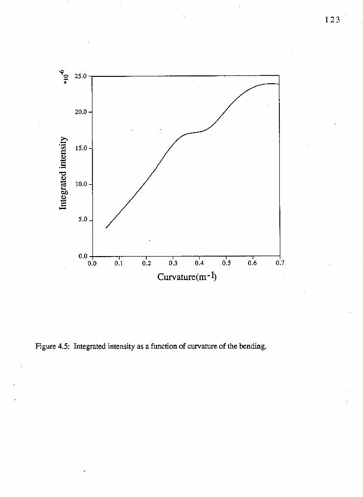
Figure 4.5: Integrated intensity as a function of curvature of the bending.

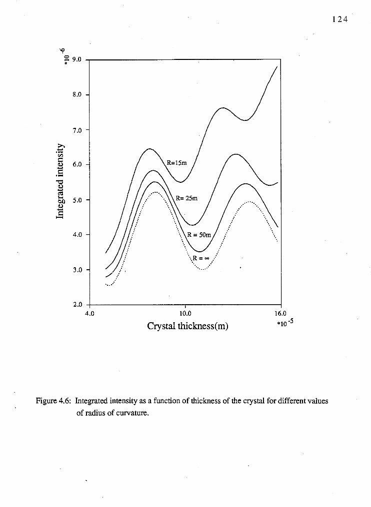
10.0 16.0

Crystal thickness(m) *lo -5

Figure 4.6: Integrated intensity as a function of thickness of the crystal for different values

of radius of curvature.

displacement fields corresponding to the type of bending created during the experiment.

This can be obtained by applying the conventional elasticity theory with boundary

conditions suitable for the experimental situation. In most situations, the displacement field

cannot be expressed accurately in terms of a second order polynomial of coordinates, i.e.

higher order polynomials are necessary to specify the displacement field adequately.

We now consider the following type of bending as an example. The method of

bending is to apply forces which determine the positions and slopes of the surfaces at two

opposite edges, leaving two edges free. For this purpose we used four aluminium rods in

pairs to create couples near each of the two edges. This bending device is illustrated in Fig.

4.7a. Under these conditions, the boundary conditions in the xyz coordinate system (see

Fig. 4.7b) are given by

where w is the z component of the mid-surface displacement vector and m is the slope of

the mid-surface at the fixed edges. Note that 2a, 2b and t are the dimensions of the crystal

plate.

In conventional elasticity theory we use the calculus of variations to produce

differential equations from the elastic energy. For simplicity, we choose Si crystals (cubic

crystal) as our model to calculate this energy. The coordinate axes are parallel to the cubic

edges which are also parallel to the edges of the crystal. Taking the elastic symmetry into

account, one can write the elastic energy per unit volume as

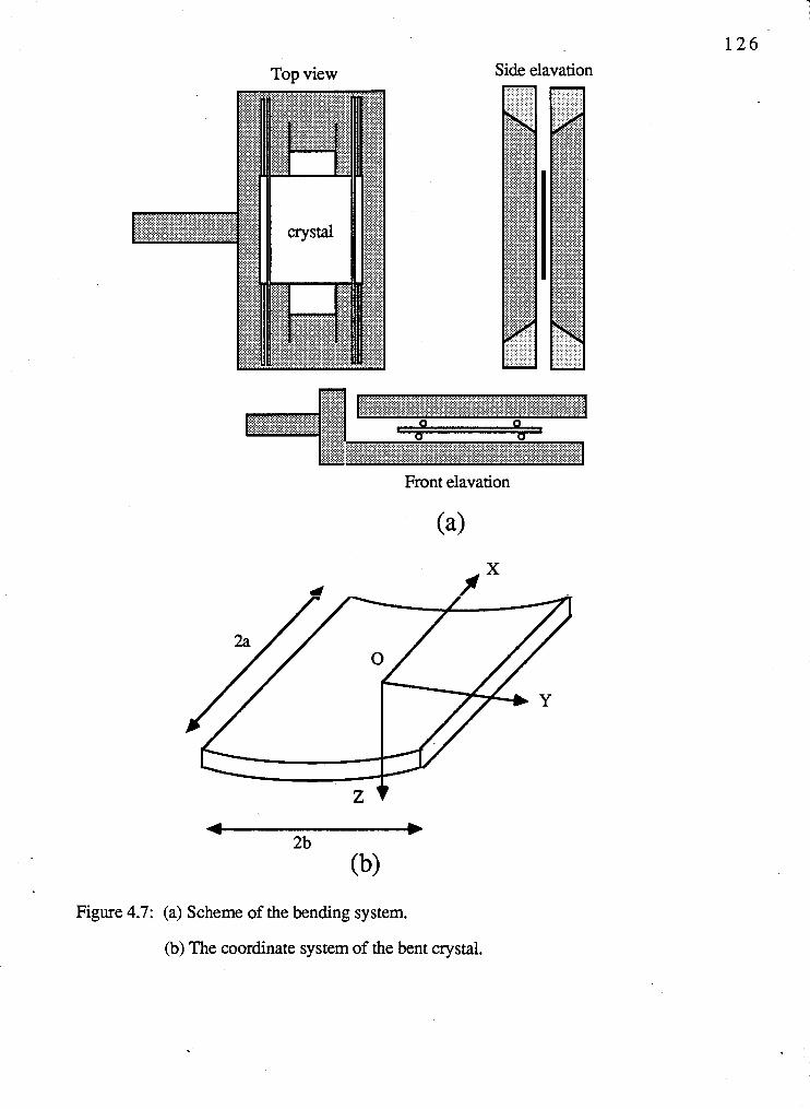
Side elavation Top view

Front elavation

(a)

Figure 4.7: (a) Scheme of the bending system.

(b) The coordinate system of the bent crystal.

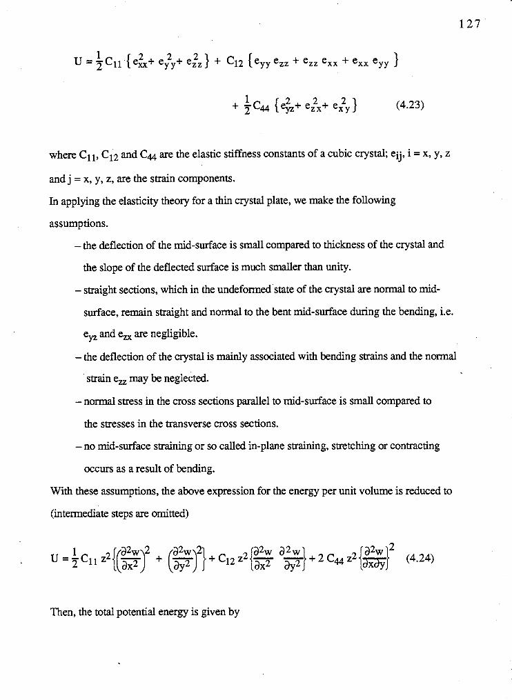
where Cll, C12 and CU are the elastic stiffness constants of a cubic crystal; eij, i = x, y, z

and j = x, y, z, are the strain components.

In applying the elasticity theory for a thin crystal plate, we make the following

assumptions.

-the deflection of the mid-surface is small compared to thickness of the crystal and

the slope of the deflected surface is much smaller than unity.

- straight sections, which in the undeformed state of the crystal are normal to mid-

surface, remain straight and normal to the bent mid-surface during the bending, i.e.

eF and e, are negligible.

- the deflection of the crystal is mainly associated with bending strains and the normal

strain e, may be negiected.

- normal stress in the cross sections parallel to mid-surface is small compared to

the stresses in the transverse cross sections.

-no mid-surface straining or so called in-plane straining, stretching or contracting

occurs as a result of bending.

With these assumptions, the above expression for the energy per unit volume is reduced to

(intermediate steps are omitted)

Then, the total potential energy is given by

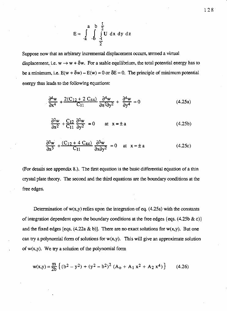
Suppose now that an arbitrary incremental displacement occurs, texmed a virtual

displacement, i.e. w -+ w + 6w. For a stable equilibrium, the total potential energy has to

be a minimum, i.e. E(w + 6w) - E(w) = 0 or 6E = 0. The principle of minimum potential

energy thus leads to the following equations:

(For details see appendix 8.). The first equation is the basic differential equation of a thin

crystal plate theory. The second and the third equations are the boundary conditions at the

free edges.

Determination of w(x,y) relies upon the integration of eq. (4.25a) with the constants

of integration dependent upon the boundary conditions at the free edges {eqs. (4.25b & c))

and the fixed edges [eqs. (4.22a & b)]. There are no exact solutions for w(x,y). But one

can try a polynomial form of solutions for w(x,y). This will give an approximate solution

of w(x,y). We try a solution of the polynomial form

Note that the boundary conditions at the fixed edges are already built in the above solution.

Because of symmetry in our bending system, there are no odd order terms of coordinates in

the above solution. By substituting the above solution of w into the eqs. (4.25), and then

equating the constant terms on both sides, we can calculate the constants Ao, A1 and A2.

The mid-surface displacement, calculated using the above expression {eq. (4.26)) of

w(x,y), is shown in Fig. 4.8a.

In the case of the isotropic thick beam considered above, the curvature of mid-surface v

due to the opposite bending was constant (= F). In our type of bending, we see from Fig.

4.8a that a similar kind of opposite bending occurs, but it is much less and is concentrated

only close to the free edges of the crystal. If we drop the term A2 x4 in the above solution

of w, the solutions will give the opposite sign to A1 and look more like the thick beam

case. The crystals that we have used in our experiments are quite good mirrors. On

bending, the reflection from the light sources can be used to see how uniform is the

displacement along the x-axis. In the experiments, the bending was obtained by tightening

five screws on each side of the crystal. The natural tendency of the crystal not to bend

uniformly was partially compensated by the experimenters. The tendency of this bending

not to be perfectly cylindrical is qualitatively explained by 'the higher order polynomial

solutions using the conventional elasticity theory, as for example eq. (4.26).

In the above described bending theory, we have neglected the strain in the z direction.

. To explain the increase in intensity on bending, the strain field in the z direction has to be

. taken into account in diffraction theory. We include the strain field in the z direction to the

first order as t(x,y)z. The displacement in the z direction becomes

Again by minimizing the total energy (similar to that shown in appendix 8) we get

and

In deriving the above expressions we have neglected the higher order terms (24 and 26)

which are small compared to z2 term. The differential equations (429), which determine

w(x,y,O), are similar to eqs. (4.25) except the coefficients are slightly different, as C11= 3

C12. Again we try a polynomial solution for w(x,y,O) in the form given by eq. (4.26) and

thereby the coefficients Ao, A1 and A2 are calculated. The mid-surface displacement

w(x,y,O), calculated using these coefficients, is shown in Fig. 4.8b. The mid-surface

displacements, calculated with and without strain in the z direction, show little difference.

The strain field in the z direction which is important in the diffraction theory, can be

calculated from eq. (4.28) with w(x,y,O) found from either eqs. (4.29) or (4.25), or from

experimental measurements of w(x,y,tI2). Of course, it is no more work to use the more

accurate form, that is eq. (4.29).

In some experimental situations, the axes of the coordinate system are not parallel to

the cubic edges. The elastic stiffness constants which enter into equations depend on the

direction of the axes of the coordinate system. If the direction of the axes is changed, then

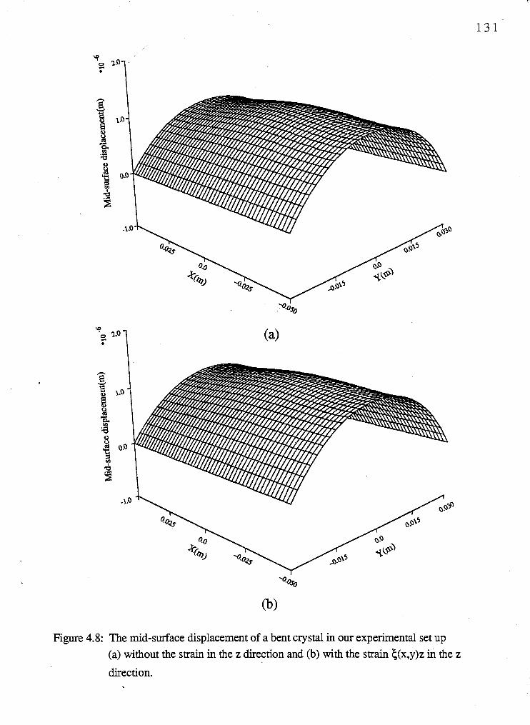
Figure 4.8: The mid-surface displacement of a bent crystal in our experimental set up (a) without the strain in the z direction and (b) with the strain c(x,y)z in the z

direction.

the elastic constants must be recalculated. One can determine the elastic constants

corresponding to the new coordinate system in terms of known elastic constants associated

with the simple coordinate system, that we have mentioned above, by finding a proper

transformation. This transformation tensor can be found using the expressions of the

elastic potential and the equations of the generalized Hooke's law with the elastic symmetry

[30]. The different sets of elastic constants are necessary to study the different types of Si

crystals ((1 11) and (100) cut wafers).

4.5 Application of uniform strain gradient solutions to the experimental

situation

The bending created in our experimental arrangements can be modeled by

conventional bending theory as explained in section 4.4. The mid-surface displacement

contains higher order terms (> second order). The local radii of curvature of the mid-

surface, Rx, Ry and Rxy,which are given by

vary position to position.

Calculating the intensity of the diffracted beam at an arbitrary point involves only the

strains in the inverse Borrmann triangle associated with that observation point. The

thickness of crystals that we used in our experiments is small compared to other

. dimensions, so the width of the Bornnann triangle is small as well. Therefore we can

assume that the strain gradient in the Borrmann triangle is uniform. This uniform strain

gradient is determined by the local radii of curvature at the center of the Borrmann triangle.

The value of uniform strain gradient varies slowly from one Borrmann triangle to other.

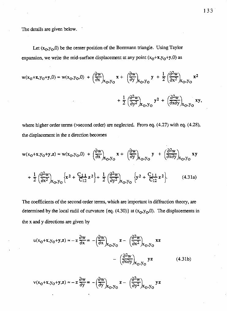
The details are given below. '

Let (xo,yo,O) be the center position of the Borrmann triangle. Using Taylor

expansion, we write the mid-surface displacement at any point (xo+x,yo+y,O) as

where higher order terms (>second order) are neglected. From eq. (4.27) with eq. (4.28),

the displacement in the z direction becomes

The coefficients of the second order terms, which are important in diffraction theory, are

determined by the local radii of curvature {eq. (4.30)) at (xo,yo,O). The displacements in

the x and y directions are given by

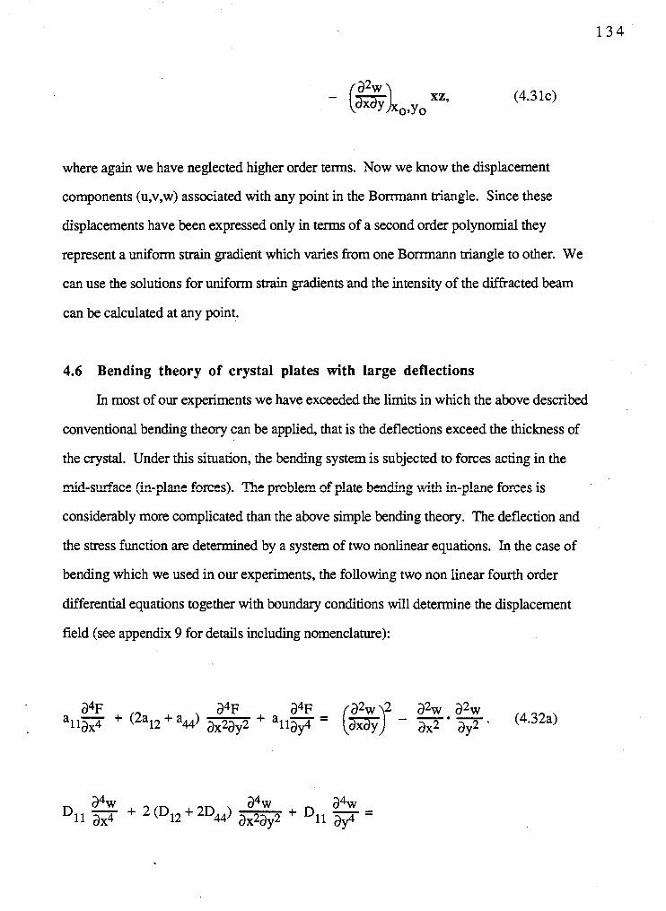
where again we have neglected higher order terms. Now we know the displacement

components (u,v,w) associated with any point in the Bomnann mangle. Since these

displacements have been expressed only in terms of a second order polynomial they

represent a uniform strain gradient which varies from one Bonmann triangle to other. We

can use the solutions for uniform strain gradients and the intensity of the diffracted beam

can be calculated at any point.

4.6 Bending theory of crystal plates with large deflections

In most of our experiments we have exceeded the limits in which the above described

conventional bending theory can be applied, that is the deflections exceed the thickness of

the crystal. Under this situation, the bending system is subjected to forces acting in the

mid-swfacp, (in-plms fcrcs). ms pr~blem ~f nlate r- bsndhqg with in -phe fmces is

considerably more complicated than the above simple bending theory. The deflection and

the stress function are determined by a system of two nonlinear equations. In the case of

bending which we used in our experiments, the following two non linear fourth order

differential equations together with boundary conditions will determine the displacement

field (see appendix 9 for details including nomenclature):

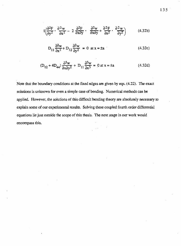
Note that the boundary conditions at the fixed edges are given by eqs. (4.22). The exact

solutions is unknown for even a simple case of bending. Numerical methods can be

applied. However, the solutions of this difficult bending theory are absolutely necessary to

explain some of our experimental results. Solving these coupled fourth order differential

equations lie just outside the scope of this thesis. The next stage in our work would

encompass this.

CHAPTER 5

SUMMARY

The dynamical theory of neutron diffraction is studied for parallel-sided perfect

crystals using the eikonal approach and the spatially dependent amplitude approach. In the

eikonal approach a given incident plane wave.generates four pairs of internal waves. The

wave vectors of these waves are found by expressing the dispersion relation in terms of *A *B *C *D

four convenient parameters &, , KO,, &, and &,. Boundary conditions at the

surfaces of the crystal determine all the unknown internal and external wave amplitudes.

The spatially dependent amplitude approach was developed because of its utility in an

approximate form called the T-T method. The spatially dependent amplitude approach

yields the same results as the eikonal method but is less convenient because of the oblique

coordinate system used in deriving the coupled differential equations. This is particularly

so for extreme cases where wave vectors are nearly parallel to surfaces.

In studying the non extreme cases some approximations are useful in both

approaches. In the eikonal approach, two pairs of internal waves suffice to describe the

propagation of neutrons in the crystal. In the T-T approach, the second derivatives of the

wave amplitudes are neglected in the coupled differential equations, using the fact that they

are slowly varying. These two approaches lead to almost the same results in most cases.

An analytical expression was obtained for the intensity of the diffracted beam in the Laue

geometry. Integrated intensity was calculated by taking the wavelength spread and the

. angular spread of the incoming beam into account. By defining new dimensionless

variables, normalized thickness and normalized intensity, we have obtained a universal

curve representing intensity as a function of thickness from which one can calculate the

period of oscillation in all possible cases of Laue transmission geometries. The

experimentally measured diffracted beam intensity as a function of thickness of Si wafers

shows good agreement with the theory.

In the extreme cases, it has been shown that three pairs of internal waves are

sufficient to describe adequately the propagation of neutrons inside the crystal. The

dynamical diffraction theory for perfect crystals given in this thesis is unique in the fullness

of the approach and its direct application to a simple and actual experimental geometry.

Using the T-T method, the solutions of the dynamical problem in the case of

homogeneously bent crystals have been expressed previously in terms of confluent

hypergeometric functions . Mathematical obscurities have been eliminated here by

expressing the confluent hypergeometric functions in terms of Chebyshev polynomials.

Calculating the amplitudes of the internal waves at an arbitrary point involves only the

strain field in the inverse Borrmann triangle associated with the observation point. In our

experiments the crystals are bent almost to a cylindrical form. The deviations are

qualitatively explained by the solutions of the conventional elasticity the&. The results

show that the strain gradient varies from position to position. However, the strain gradient

can be treated as uniform in each Bomnann triangle for the Si wafers that we used in our

experiments. The local strain gradients are determined by the local radii of curvature at the

center point of the Borrmann triangles. The local radii of curvature, which vary from one

Bomnann triangle to other, either can be calculated from the mid-surface displacement

obtained using the conventional elasticity theory or measured experimentally. By knowing

the value of uniform strain gradient in the Borrmann triangle, we can calculate the internal

wave amplitudes at any point.

In some experiments we have exceeded the limits in which the conventional elasticity

theory can be applied. In this situation, two coupled non linear fourth order differential

equations determine the mid-surface displacement.

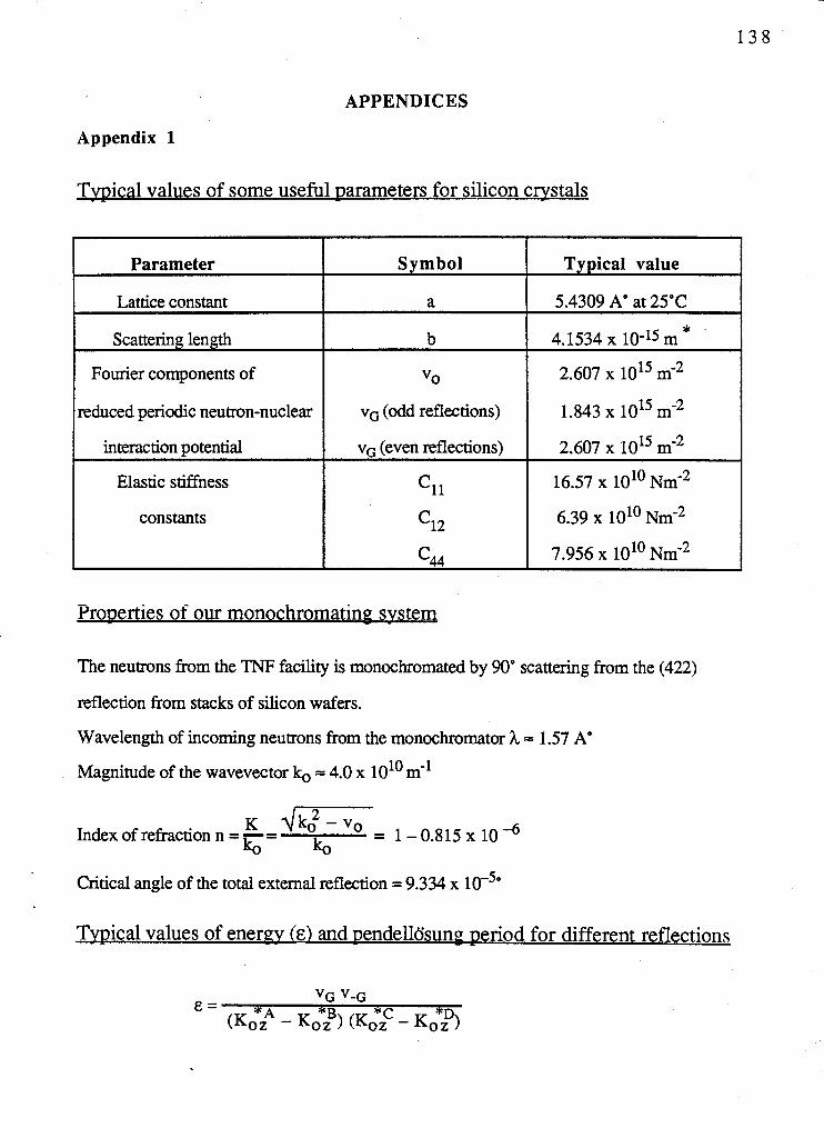
APPENDICES

Appendix 1

Twical values of some useful Darameters for silicon crystals

Parameter

Lattice constant

Scattering length

Fourier components of

reduced periodic neutron-nuclear

interaction ~otential

Elastic stiffness

constants

Symbol

vG (odd reflections)

vc, (even reflections)

Typical value

5.4309 A' at 25•‹C

Yro~erties of our monochromating svstem

The neutrons from the TNF facility is monochromated by 90" scattering from the (422)

reflection from stacks of silicon wafers.

Wavelength of incoming neutrons from the monochromator h = 1.57 A"

10 -1 Magnitude of the wavevector k, = 4.0 x 10 m

K l /k&vo Index of refraction n = - = k, k,

= 1-0.815 x l o 4

Critical angle of the total external reflection = 9.334 x

Tpical values of energy (&) and pendelltSsung ~ e r i o d for different reflections

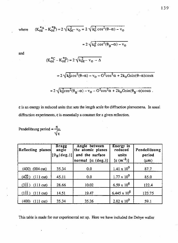
where ( ~ ~ * ~ - < ~ ) = 2 ~ ~ = 2 . \ 1 ~ ~ 0 s ~ ( e - a ) - ~ ~

and

E is an energy in reduced units that sets the length scale for diffraction phenomena. In usual

diffraction experiments, E is essentially a constant for a given reflection.

n; PendellCjsung period = - 6

Reflecting planes

(400) (004 cut)

(422, (111 cut,

(400) (1 11 cut)

Angle between the atomic planes and the surface

normal [a (deg.)]

0.0

units I period I

Energy in reduced

This table is made for our experimental set up. Here we have included the Debye waller

Pendellosung

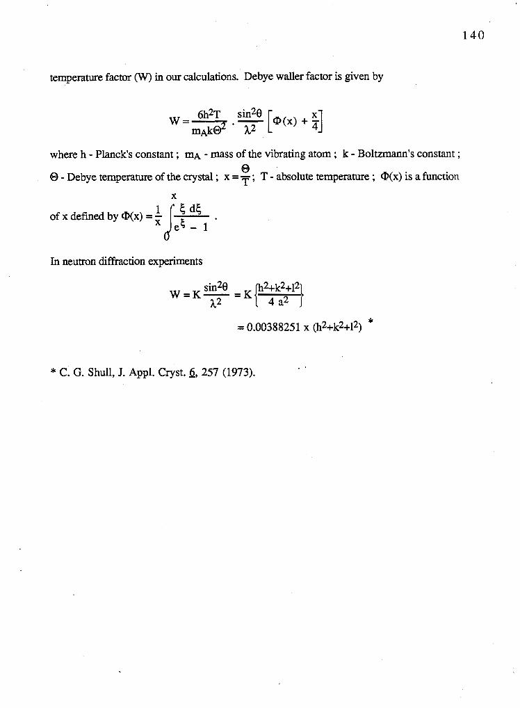
temperature factor (W) in our calculations. Debye waller factor is given by

where h - Planck's constant ; mA - mass of the vibrating atom ; k - Boltmann's constant ; 0

8 - Debye temperature of the crystal ; x = T ; T - absolute temperature ; Q(x) is a function

X

of x defined by cP(x) = -

In neutron diffraction experiments

. - * C. G. Shull, J. Appl. Cryst. 6, 257 (1973).

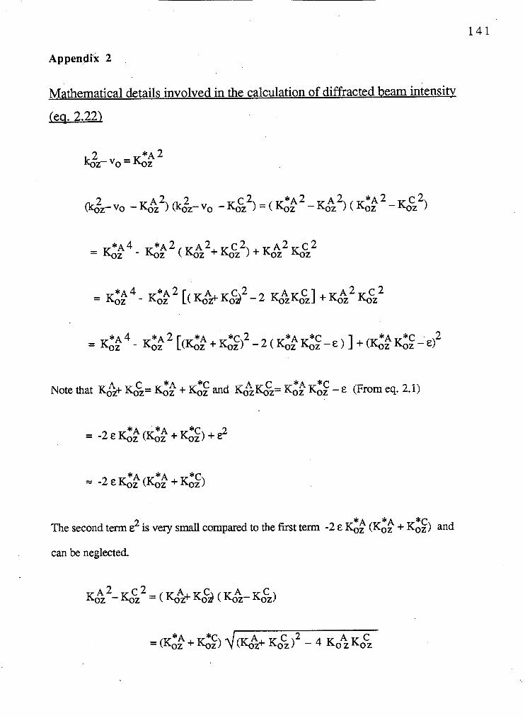
Mathematical details involved in the calculation of diffracted beam intensity

(ea. 2.22)

The second term e2 is very small compared to the fust term -2 E gk (Id: + KG:) and

can be neglected.

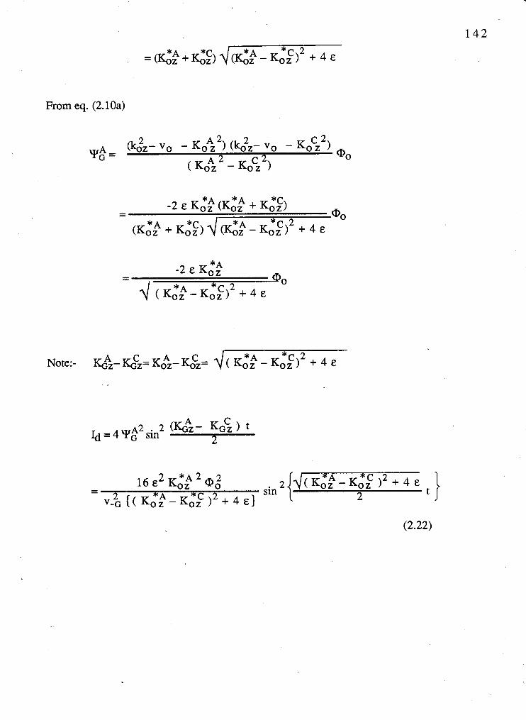
From eq. (2.10a)

~2 2 Id = 4 YG sin

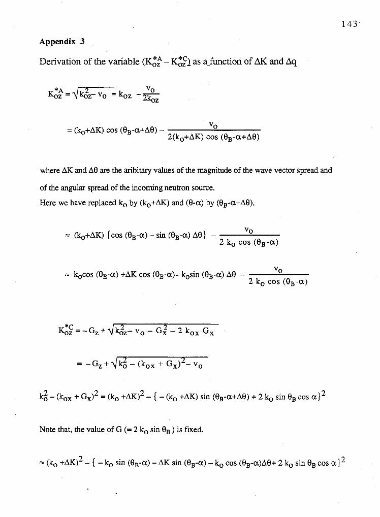
Appendix 3

Derivation of the variable (IS:$ - K,*$) as afunction of AK and Aq

where AK and A8 are the aribitary values of the magnitude of the wave vector spread and

of the angular spread of the incoming neutron source.

Here we have replaced ko by (b+AK) and (8-a) by (eB-a+A8).

{cos (BB-a) - sin @,-a) A@) - vo 2 ko COS ( 8 ~ - a )

vo 2 ko cos (QB-a)

ki - (kox + G , ) ~ = (ko + A K ) ~ - { - (ko +AK) sin ( B ~ - ~ + A B ) + 2 sin BB cos a} 2

Note that, the value of G (= 2 ko sin eB ) is fixed.

= (ko + A K ) ~ - { - kg sin (eB-a) - AK sin (eB-a) - ko cos (eB-a)A8+ 2 ko sin eg cos a } 2

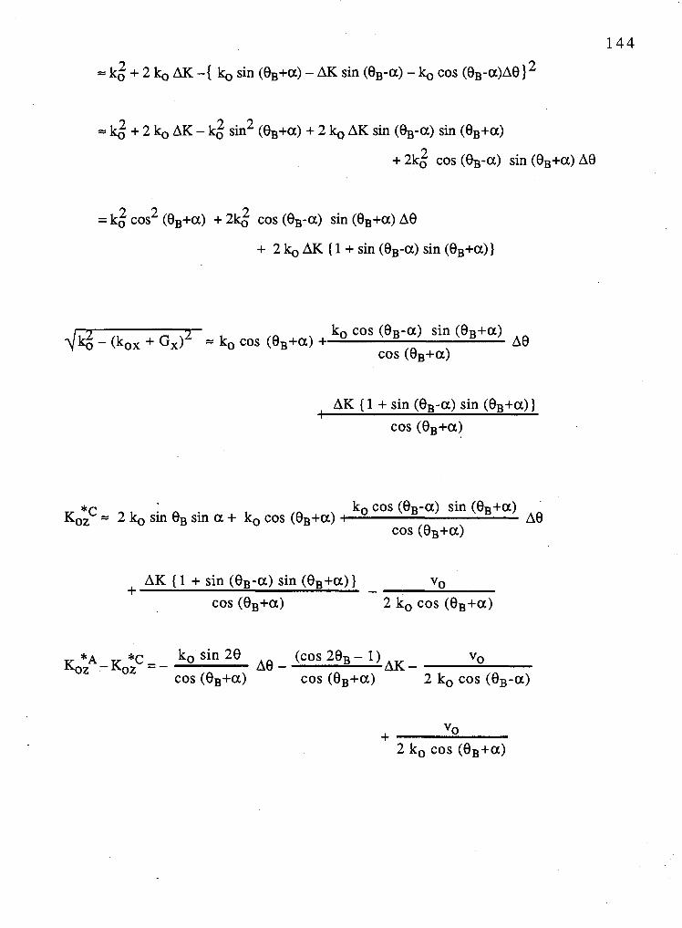
2 2 - 2 = ko + 2 k, AK - k, sin (eB+a) + 2 k, AK sin (eB-a) sin (eB+a)

+ 2162 cos (eB-a) sin (eB+a) AB

2 2 2 = ko COS (eB+a) + 2k, COS (eB-a) sin (eB+a) A 8

+ 2 k, AK (1 + sin (eB-a) sin (eB+a))

ko COS (eB-a) sin (eB+a) d k g - (kox + G , ) ~ = ko cos (BB+a) + A0

cos (eB+a)

, AK { 1 + sin (8B-a) sin (eB+a) ) I

cos (eB+a)

ko COS (oB-a) sin (eB+a) K,*,C = 2 ko sin 8, sin a + ko cos (eB+a) : At3 cos (eB+a)

*c , ko sin 28 (COS 2eB - - -- A8 - ' )AK-

vo cos (eB+a) cos (eB+a) 2 ko cos (eB-a)

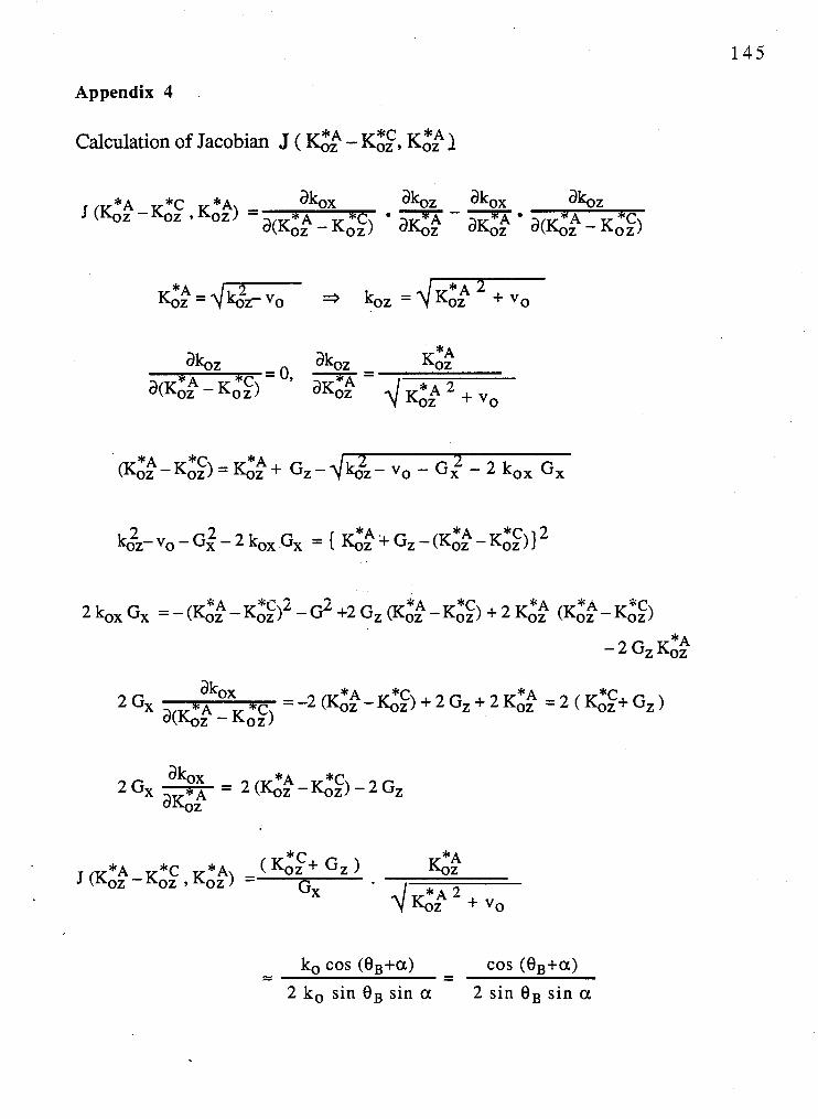
Appendix 4

Calculation of Jacobian J ( e k - K ~ ~ , K:; 1

*A - J ( G k - G , C ,KO,) - akox akoz akox

C '*A-** akoz

a c e - ~ , * z aKoz a ( G - K,I,C)

a b z akoz =o, *A= K:,A a ( ~ 2 - K,*$) a K ~ ~ 4 K:; + vo

- ko COS (eB+a) - - cos ( eB+a) - 2 ko sin eB sin a 2 sin eB sin a

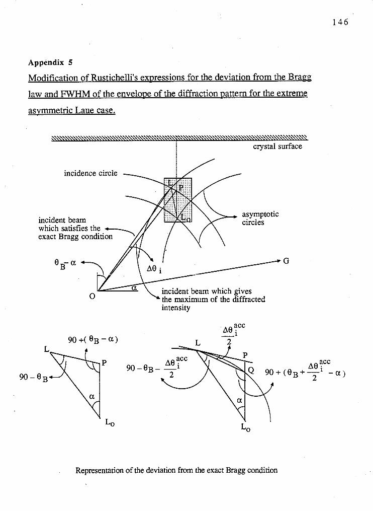
Appendix 5

Modification of Rustichelli's expressions for the deviation from the Bragrz,

law and FWHM of the envelope of the diffraction vattern for the extreme

asvrnrnetric Laue case.

crystal surface

incidence circle

asymptotic incident beam circles which satisfies the exact Bragg conditi

0 incident beam which gives the maximum of the diffracted intensity

A0 yc

Representation of the deviation from the exact Bragg condition

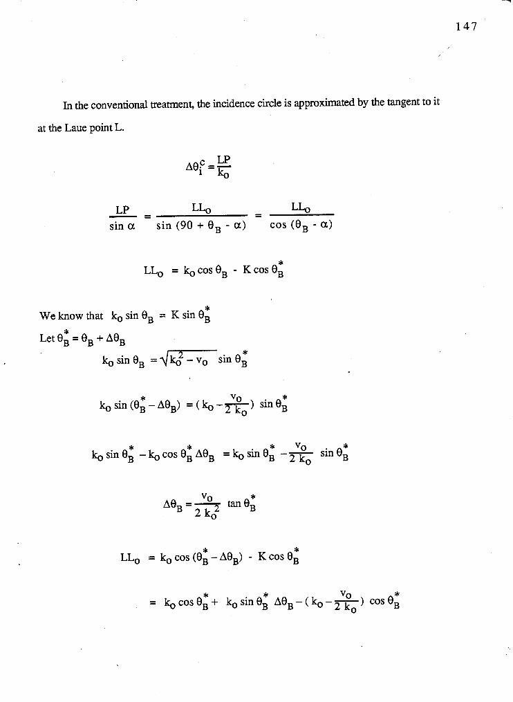
In the conventional treatment, the incidence circle is approximated by the tangent to it

at the Laue point L.

LP - = LLo - - LL, sin a sin (90 + B B - a) cos (BB - a)

* We know that k, sin BB = K sin BB

* Let BB = BB + ABB

* k, sin Bg = sin BB

* * ) sin eB k,sin(BB-AeB) =(k,--

2 ko

* * * * sin eB k,sinBB -k,cosBBABB =kosinBB -=

vo ABB = - tan 0; 2 k,2

* * LLo = ko cos (BB - ABB) - K cos BB

* * vo * = kOcosBB + k0sineB A e B - ( k 0 - r n ) cosBB

0

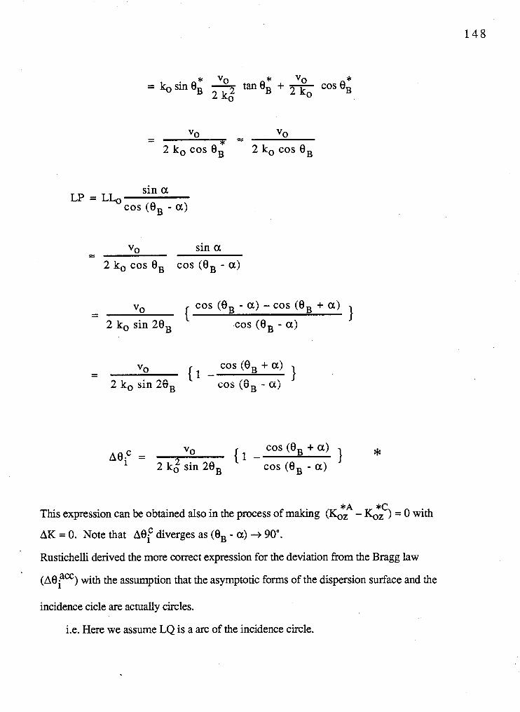
* * "0 V0 tan eB + - = k, sin eB -

2 k,2 2 ko

sin a LP = LLo

cos (eB - a)

- vo sin a - 2 ko cos OB cos (eB - a)

vo { cos (€IB - a) - cos (eB + a) - -

2 ko sin 2eB cos (€IB - a) I

Vo cos (€IB + a) A e f = 2 k,2 sin 2eg

( 1 - cos (€IB - a) I *

*A *C This expression can be obtained also in the process of making O(oz - Koz ) = 0 with

AK = 0. Note that ~ 8 ; diverges as (€IB - a) + 90'. Rustichelli derived the more correct expression for the deviation from the Bragg law

(Aeiacc) with the assumption that the asymptotic forms of the dispersion surface and the

incidence cicle are actually circles.

i.e. Here we assume LQ is a arc of the incidence circle.

- arc LQ 1 - k,

LLo w = - A € I ~ sin a

sin (90 + [€IB + - al)

Aeyc 2 ko sin ( )

" - - - A € I ~ sin a

2 ko cos €IB cos (€IB + - a)

heyc vo - 2 k o ( 2 ) -

A€IfcC sin a 2 kn w cos 8, (cos (€IB - a) - sin (Bg - a)

D 2 1

A(-) .act 1

~ e a c c ) +

vo sin a sin (€IB - a) ( )2 - cos (€IB - a) ( 2 = O

4 k i cos €IB

where yl = cos (BB - a) and y2 = cos (BB + a)

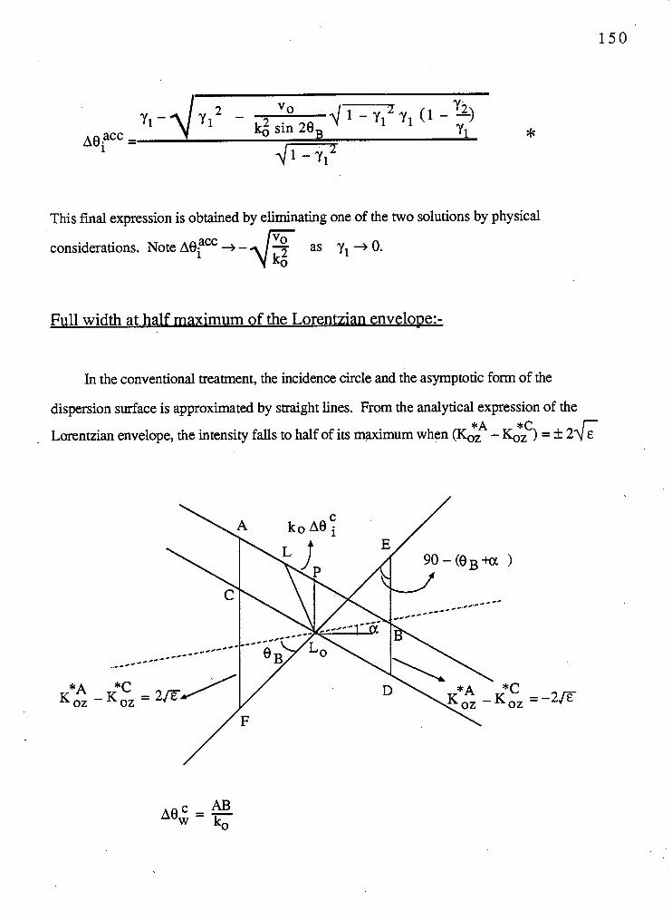
This final expression is obtained by eliminating one of the two solutions by physical

considerations. Note heiaCC + - a as yl + 0.

Full width at half maximum of the Lorentzian envelope:-

In the conventional treatment, the incidence circle and the asymptotic form of the

dispersion surface is approximated by straight lines. From the analytical expression of the *A *C

Lorentzian envelope, the intensity falls to half of its maximum when (Koz - KO, ) = k 2 6

1 AB = CD, CLo = DLo = 2 CD

ED - - w - - w sin 28, sin [90 - (eB + a)] cos (8, + a)

ED =2&= VG

ko d c o s (8, - a) cos (8, + a)

ko 4 cos (8, - a) cos (8, + a) sin 2gB

- - ko sin 29, cos (OB - a)

~8; = * cos (8, - a)

*A *C 2 This expression can be obtained also from the condition (G, - KO, ) = 4 E with

AK = 0.

For AB<< ko, it is also valid to a good approximation that

Lp = = "0 (1-a) 2 k, sin 28, Y1

Note that AOFC + 0 as yl + 0.

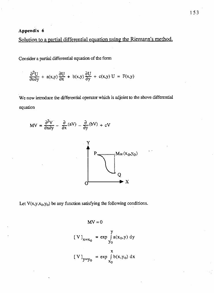
Appendix 6

Solution to a partial differential eauation using the Riemann's method.

Consider a partial differential equation of the form

We now introduce the differential operator which is adjoint to the above differential

equation

Let V(x,y,xo,yo) be any function satisfying the following conditions.

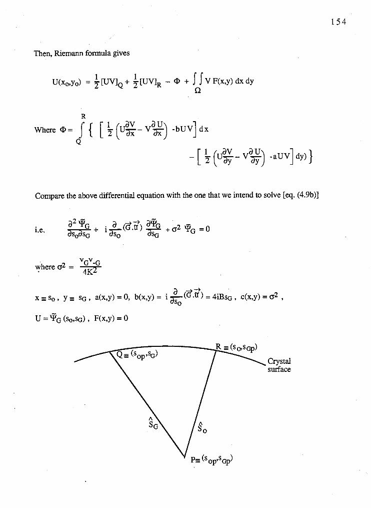
Then, Riemann formula gives

Compare the above differential equation with the one that we intend to solve [eq. (4.9b)l

where 02 - v ~ v - ~ 4 I C 2

Crystal surface

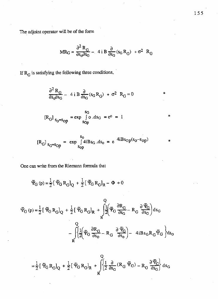
The adjoint operator will be of the form

If RG is satisfying the following three conditions,

so = exp I 4iBsG .dso = e 4 i B ~ ~ ~ ( s ~ - s o ~ ) lRG1 SG=SG~

. . One can write from the Riemann formula that

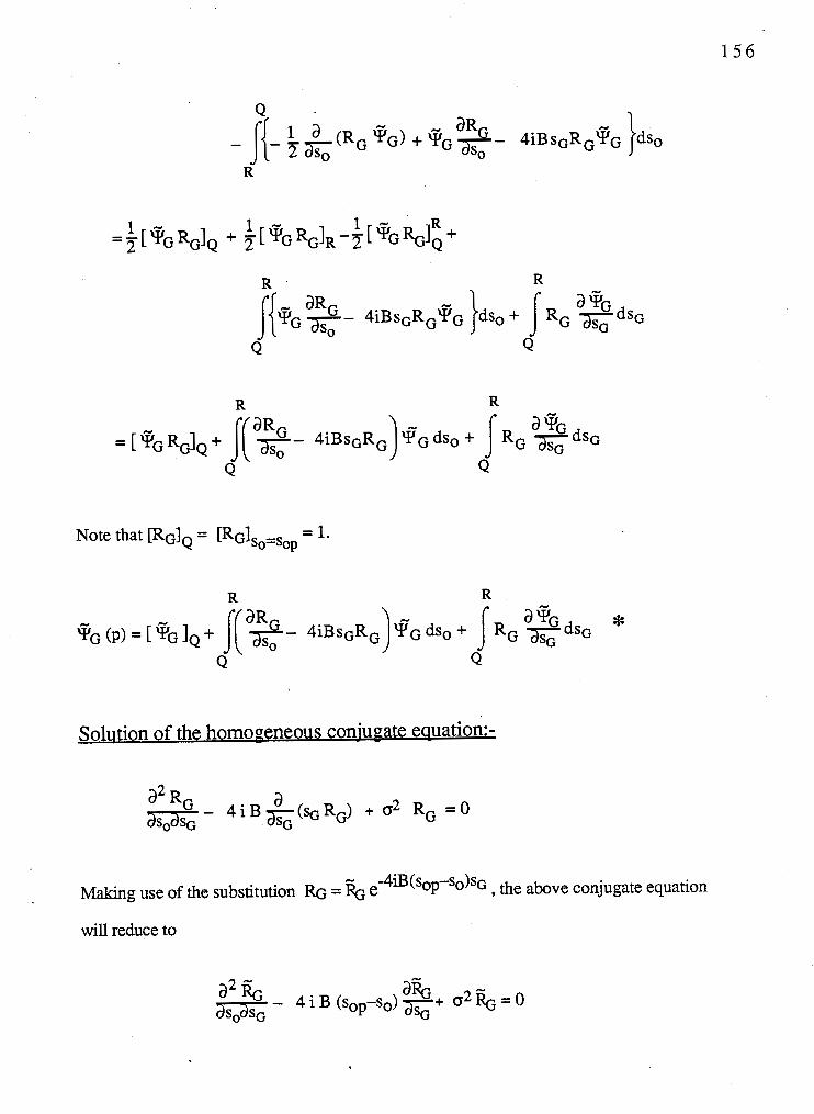
~ S G * qG (p) = ( - ~~BSGRG)'G dso + j R G

Q Q

Solution of the homoaeneous conjugate emation:-

Making use of the substitution RG = & e -~~B(so~-so)sG th

will reduce to

[e abov .e conjugate equati

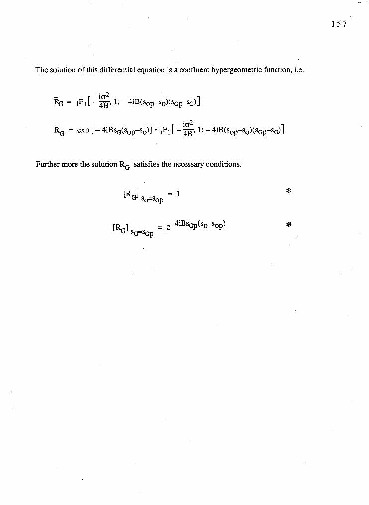
The solution of this differential equation is a confluent hypergeometric function, i.e.

Further more the solution RG satisfies the necessary conditions.

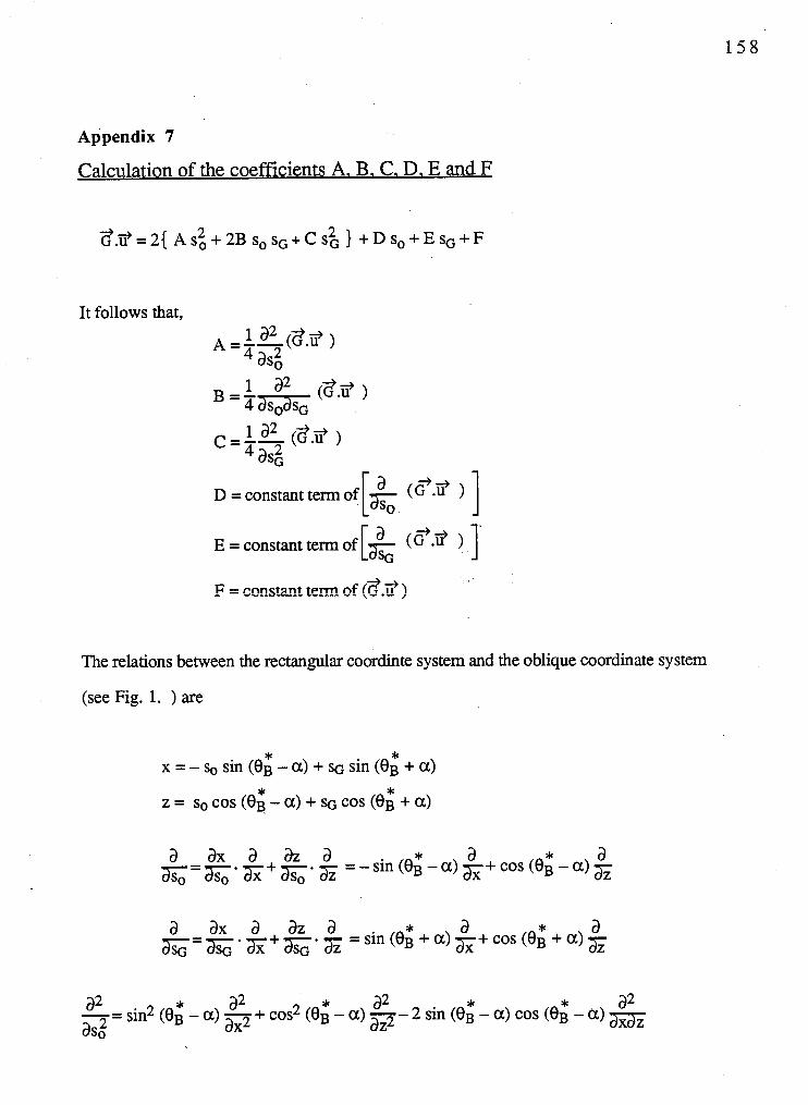
Appendix 7

Calculation of the coefficients A. B, C. D. E and F

It follows that,

D = constant term of (G JJ ) K O " I [ tG (g.3 ) 1' E = constant term of

F = constant term of (3.3 )

The relations between the rectangular coordinte system and the oblique coordinate system

(see Fig. 1. ) are

* * x = - so sin (€IB - a) + SG sin (eB + a) * *

z = so cos (€IB - a) + SG cos (eB + a)

a2 * a2 * a2 * * a2 -- sin2 (eB - a) - + cos2 (€IB - a) -- 2 sin (Bg - a) cos (OB - a) a x as$ - ax2 az2

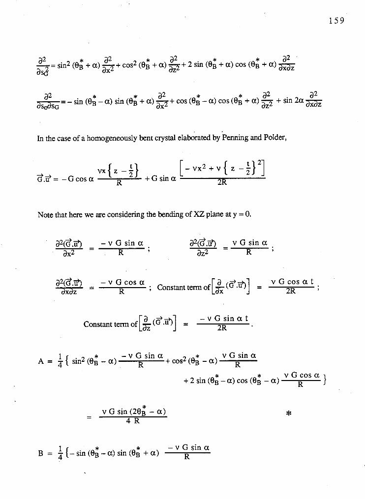
a2 * a2 * a2 * * a2 -= sin2 (eB + a) -+ cos2 (€IB + a) -+ 2 sin (BB + a) cos ( 8 ~ + a) as2 ax2 az2

a2 * * a* * * a2 a2 ZG = - sin (eB - a) sin (BB + a) - + cos (BB - a) cos (BB + a) - + sin 2a a x

ax2 az2

In the case of a homogeneously bent crystal elaborated by penning and Polder,

Note that here we are considering the bending of XZ plane at y = 0.

az(Z.i?) - - v ~ c o s a ; constant term of[& ( 2 . 3 1 = v G cos a t axaz- R 2R 9

Constant term of [$ ($.a] = - v G s i n a t

2R

1 * - v G sin a * v G sin a A = 4 { sin2 (eB - a) R + cos2 (eB - a) R

* * v G cos a + 2 sin (BB - a) cos (eB - a) I

* - - v G sin ( 2 8 ~ - a)

4 R

1 * * - v G sin a B = {- sin (eB - a) sin (eB + a) R

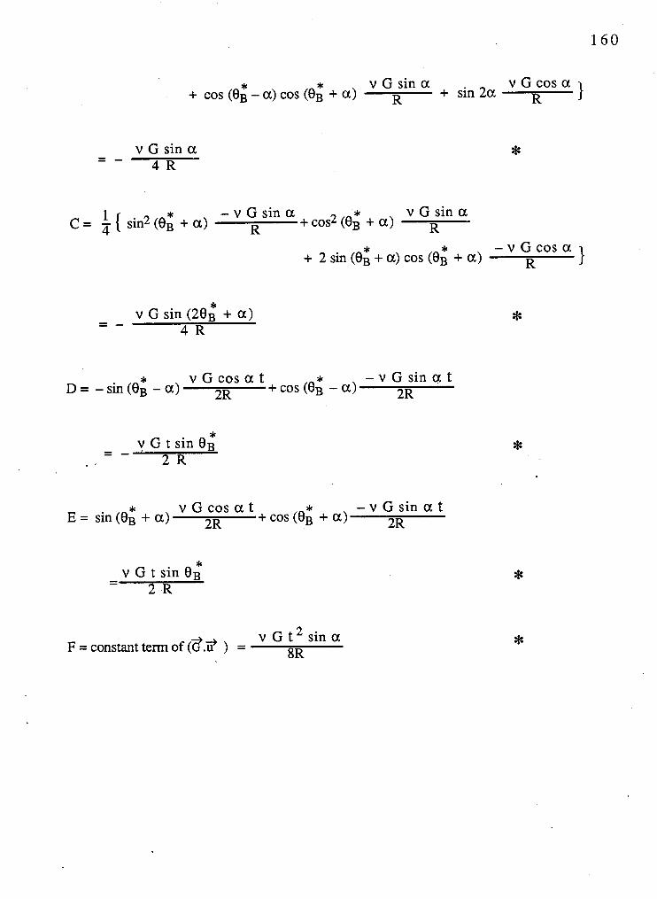
* * v G sin a v G cos a + cos (eB - a ) cos (eB + a) + sin 2 a 1

- - - v G sin a * 4 R

1 * - v G sin a v G sin a C = 7 { sin2 (OB + a ) R + cos2 (8: + a ) R

* * - v G cos a + 2 sin (eB + a ) cos (eB + a ) R 1

* v G cos a t * - v G s i n a t D= -sin(eB - a ) 2R + cos (€IB - a ) 2R

* - - - v G t sin eB

2 R

* v G cos a t - v G s i n a t E = sin (eB + a ) 2R + cos (0; + a) 2R

- v G t sin 0; - 2 -R

v G t 2 s i n a F = constant term of (3.3 ) = 8R

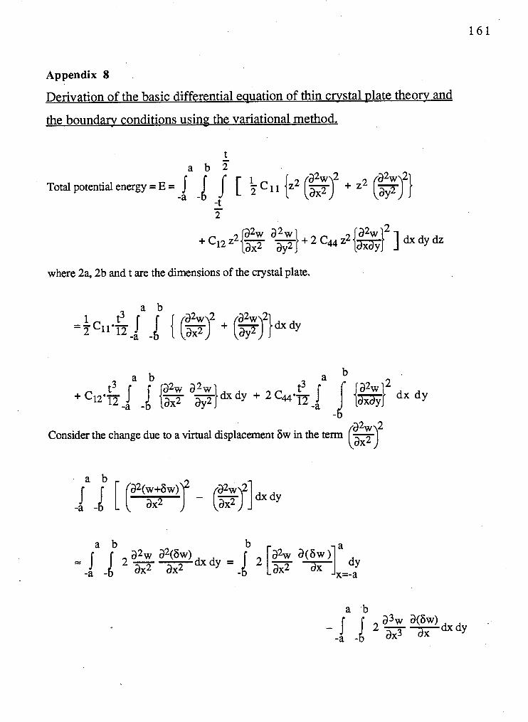
Appendix 8

Derivation of the basic differential equation of thin cnrstal date theorv and

the boundary conditions us in^ the variational method.

a b 7 a2w 2 a 2 ~ 2

Totalpotential energy = E = 1 1 I [ \ C 1 {z2 (=) + z2 (p-) } -a - -t

where 2% 2b and t are the dimensions of the crystal plate.

Consider the change due to a virtual displacement 6w in the term - (zr

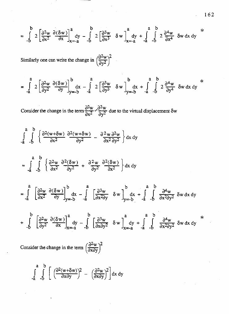
Similarly one can write the change in - ($7

a 2 ~ a 2 ~ Consider the change in the term- - due to the virtual displacement 6w

ax2 ay2

a a b a b aiw a(sw)] - - . d x - a 4 ~

a3w S w b ax2ay2 [s 7 = [- 6w dx dy -a ly=-b -a -

Consider the change in the term (a:;r

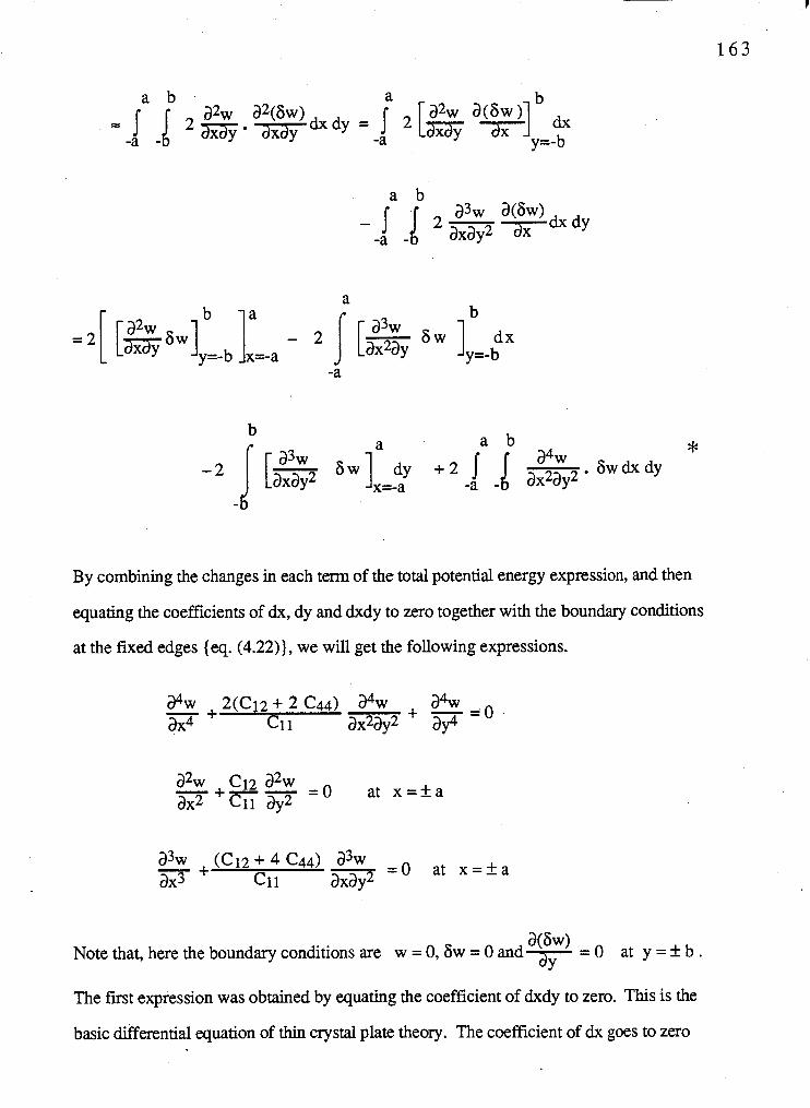
By combining the changes in each terrn of the total potential energy expression, and then

equating the coefficients of dx, dy and dxdy to zero together with the boundary conditions

at the fixed edges {eq. (4.22)), we will get the following expressions.

Note that, here the boundary conditions are w = 0,6w = 0 and W w ) 7 = O at y = + b .

The first expression was obtained by equating the coefficient of dxdy to zero. This is the

basic differential equation of thin crystal plate theory. The coefficient of dx goes to zero

automatically. The second and the third equations are the boundary conditions at the free

edges which are obtained by equating the coefficient of dy to zero.

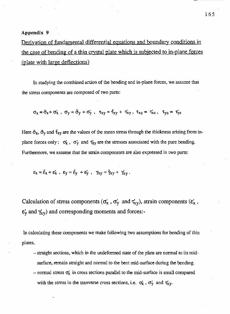
Appendix 9

Derivation of fundamental differential equations and boundary conditions in

the case of bending of a thin crystal plate which is subiected to in-plane forces

(plate with large deflections)

In studying the combined action of the bending and in-plane forces, we assume that

the stress components are composed of two parts:

Here ex, ey and fxy are the values of the mean stress through the thickness arising from in-

plane forces only ; & , o$ and zky are the stresses associated with the pure bending.

Furthermore, we assume that the strain components are also expressed in two parts:

Calculation of stress components (a; , a; and Gy), strain components (E; ,

E; and Yxy) and corresponding moments and forces:-

In calculating these components we make following two assumptions for bending of thin

plates.

- straight sections, which in the undeformed state of the plate are normal to its mid-

surface, remain straight and normal to the bent mid-surface during the bending.

- normal stress oi in cross sections parallel to the mid-surface is small compared

with the stress in the tranverse cross sections, i.e. & , oj, and ziy.

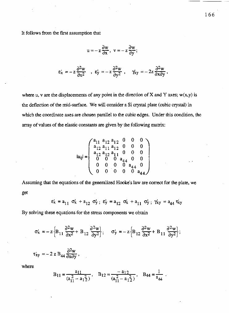
It follows from the first assumption that

where u, v are the displacements of any point in the direction of X and Y axes; w(x,y) is

the deflection of the mid-surface. We will consider a Si crystal plate (cubic crystal) in

which the coordinate axes are chosen parallel to the cubic edges. Under this condition, the

array of values of the elastic constants are given by the following matrix:

Assuming that the equations of the generalized Hooke's law are correct for the plate, we

By solving these equations for the stress components we obtain

where

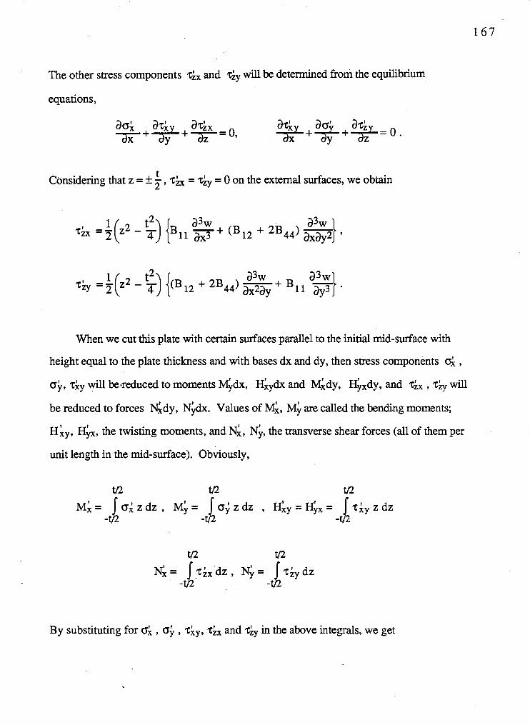
The other stress components 6, and Gy will be determined from the equilibrium

equations,

t Considering that z = f - , z& = Gy = 0 on the external surfaces, we obtain 2

When we cut this plate with certain surfaces parallel to the initial mid-surface with

height equal to the plate thickness and with bases dx and dy, then stress components c& ,

o i , 7iy will be~reduced to moments Midx, H & ~ X and ~ ; d y , ~;,dy, and GX , rS will

be reduced to forces &dy, N&. Values of M;, M; are called the bending moments;

H , ~ , Hi,, the twisting moments, and N;, N;, the transverse shear forces (all of them per

unit length in the mid-surface). Obviously,

By substituting for o;( , oi , 7ky, r& and Gy in the above integrals, we get

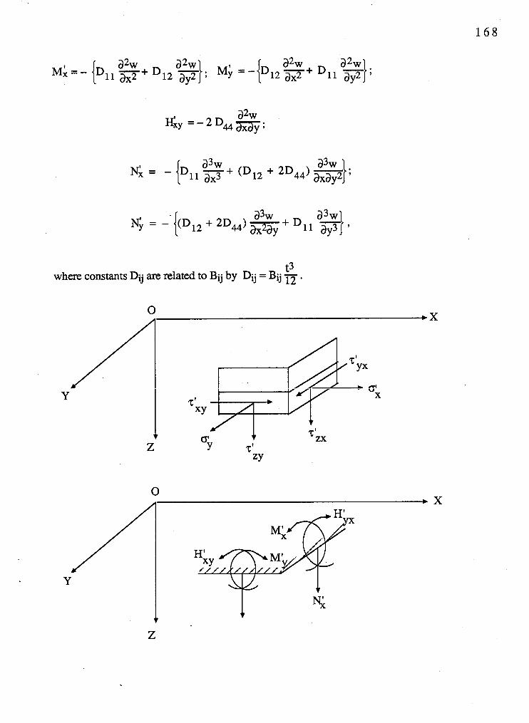
t3 where constants Dij are related to Bij by Dij = Bij .

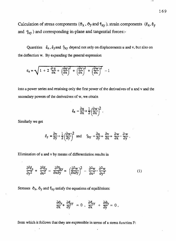
Calculation of stress components (6, , ay h d Zxy ), strain components (Ex, CJy

and Txy ) and corresponding in-plane and tangential forces:-

Quantities $, Eyand % depend not only on displacements u and v, but also on

the deflection w. By expanding the general expression

into a power series and retaining only the first power of the derivatives of u and v and the

secondary powers of the derivatives of w, we obtain

Similarly we get

Elimination of u and v by means of differentiation results in

Stresses ex, ey and fxy satisfy the equations of equilibrium:

from which it follows that they are expressible in terms of a stress function F:

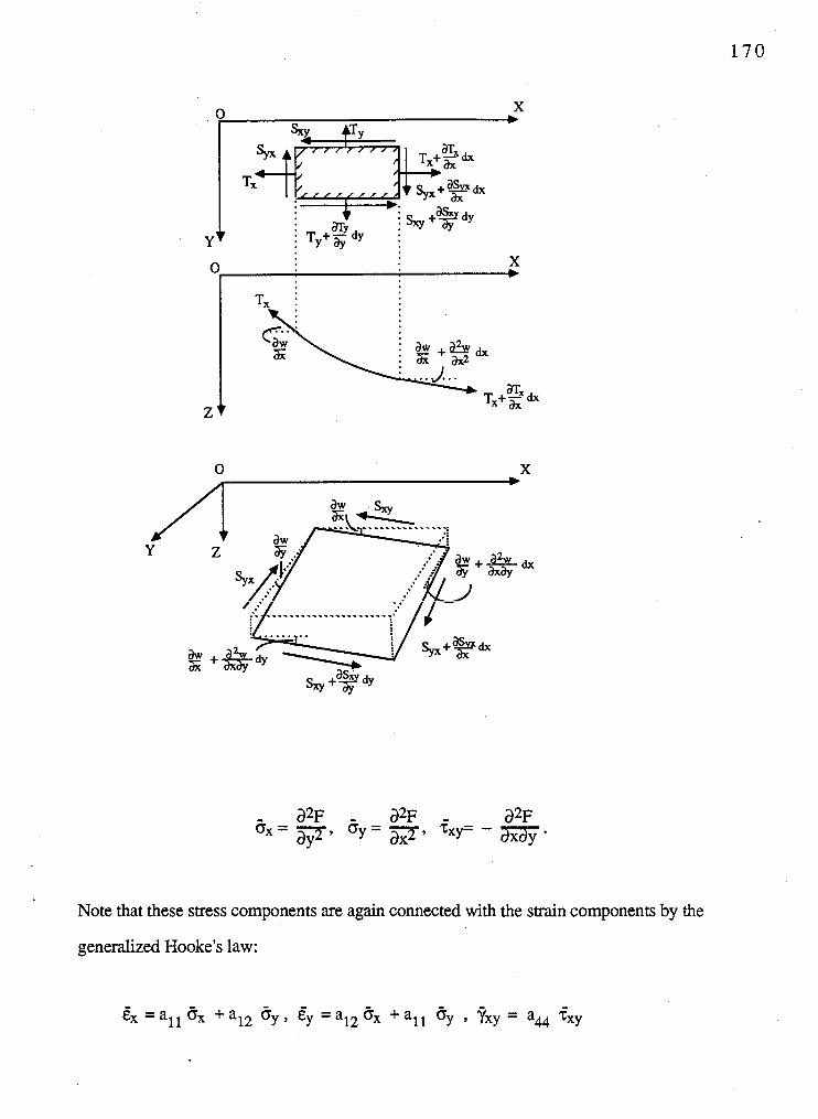
Note that these stress components are again connected with the strain components by the

generalized Hooke's law:

Ex =al , 5x +al2 Er,

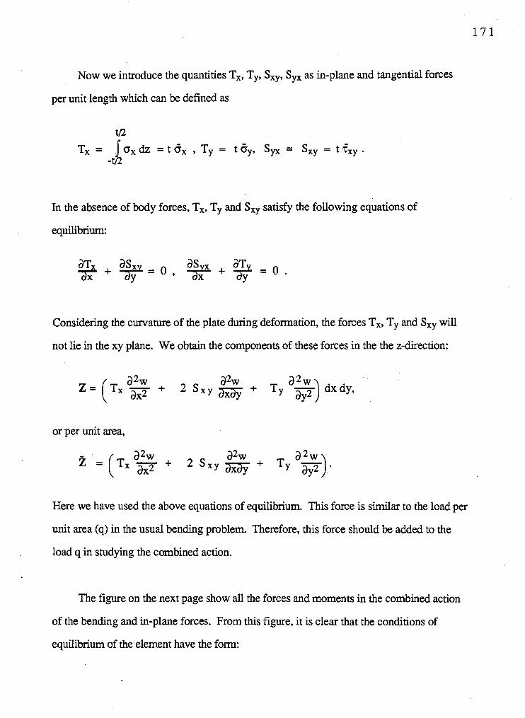
Now we introduce the quantities Tx, Ty, Sxy, Syx as in-plane and tangential forces

per unit length which can be defined as

In the absence of body forces, Tx, Ty and Sxy satisfy the following equations of

equilibrium:

Considering the curvature of the plate during deformation, the forces Tx, Ty and Sxy will

not lie in the xy plane. We obtain the components of these forces in the'the z-direction:

or per unit area,

Here we have used the above equations of equilibrium. This force is similar to the load per

unit area (q) in the usual bending problem. Therefore, this force should be added to the

load q in studying the combined action.

The figure on the next page show all the forces and moments in the combined action

of the bending and in-plane forces. From this figure, it is clear that the conditions of

equilibrium of the element have the form:

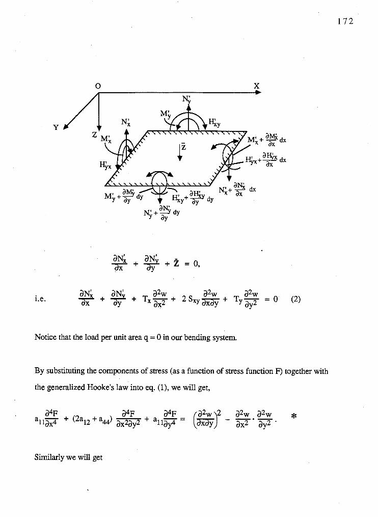
Notice that 1

a ~ ; , ax

:he loa d per unit area q = 0 in our bending system.

By substituting the components of stress (as a function of stress function F) together with

the generalized Hooke's law into eq. (I), we will get,

Similarly we will get

from eq. (2). The solutions of these two coupled non-linear differential equations

determine the deflection w and the stress function F.

Boundary conditions: -

At the supported edges (y = + b) in our bending system,

At the free edges (x = + a), Mx = 0, where

Furthermore, N; + ?* = 0 at the free edges, where

REFERENCES

[I] W. H. Zachariasen, Theory of X-rav Diffraction in Crystals, John Wiley and Sons,

London, 1945.

[2] R. W. James, The &tical Princiwles of the Diffraction of X-Rays, Bell and Sons,

London, 1950.

[3] L. V. Azarov, R. Kaplow, N. Kato, R. J. Weiss, A. J. C. Wilson and R. A.

Young, X-Ray Diffraction, Chapters 3 ,4 and 5, McGraw-Hill, London, 1974.

[4] C. G. Shull, Phys. Rev. Lett. 21, 1585 (1968).

[5] V. F. Sears, Can. J. Phys.3, 1261 (1978).

[6] H. Rauch and D. Pertaschek in Neutron Diffraction, ed. H. Dachs, Springer, Berlin

(1978), pp. 303-35 1.

[7] S. A. Werner, R. R. Berliner and M. Arif, Physica 137B, 245 (1986).

[8] S. Takagi, Acta Cryst. 15, 1131 (1962); J. Phys. Soc. Japan 26, 1239 (1969).

[9] D. Taupin, Bull. Soc. Franc. Mineral Crist. 87,469 (1964).

[lo] S. A. Werner, Phys. Rev. m, 1774, (1980).

[I 11 F. N. Chukhovskii and P. V. Petrashen, Acta Cryst. a, 31 1 (1977).

[12] S. G. Lekhnitskii, Anisotropic plates, (trans. S. W. Tsai & T. Cheron), Gordon and

Breach Science Publishers, New York (1968), pp. 273-292.

[13] S. Slobodetskii and F. N. Chukhovskii, Sov. Phys. Cryst. 15,963 (1971); J. Arthur

and M. A. Home, Phys. Rev. m, 5747 (1985); J. Arthur, C. G. Shull and A.

Zelinger, Phys. Rev. m, 5753 (1985).

[14] S. Kishino and K. Kohra, Japan J. app. Phys. 10, 551 (1971).

[15] 0. Briimmer, H. R. Hiiche and J. Nieber, Phys. Stat. Sol. &3, 587 (1976).

[16] 0. Briimmer, H. R. Hiiche and J. Nieber, Phys. Stat. Sol. m, 529 (1976).

[17] A. Zeilinger and T. J. Beatty. Phys. Rev. m, 7239 (1983).

[18] S. Kishino , J. Phys. Soc. Japan 3, 1168 (1971).

[19] T. ~ e d y h k a , Phys. Stat. Sol. m, 365 (1973).

[20] S. Kishino, A. Noda and K. Kohra, J. Phys. Soc. Japan 33, 158 (1972).

[21] T. ~ e d ~ h k a , Phys. Stat. Sol. &, 405 (1974).

[22] J. Hiirtwig, Phys. Stat. Sol. m, 417 (1976).

[23] 1. Hiirtwig,.Phys. Stat. Sol. &, 495 (1977).

[24] F. Rustichelli, Phil. Mag. 3, 1 (1975).

[25] P. Penning and D. Polder, Phylips. Res. 16,419 (1961).

[26] N. Kato, J. Phys. Soc. Japan 19, 97 1 (1964).

[27] S. L. Sobolev, Partial differential equations of Mathematical Physics, pp. 58-71.

1281 Enrico Volterra and J. H. Gaines, Advances Strength of Materials, pp. 212-214.

[29] Y. L. Luke, Akorithms for the computation of mathematical functions (1977), pp.

70-76.

[30] S. G. Lekhnitskii, Theorv of elasticitv of an inisotropic elastic body, ed. J.

Brandstatter (trans. P. Fern), Holden-Day , Inc., San Francisco (1 963), pp. 32-40.