Embed Size (px)
Citation preview
Dynamical Systems Method for Solving
Ill-conditioned Linear Algebraic Systems
Sapto W. IndratnoDepartment of Mathematics
Kansas State University, Manhattan, KS 66506-2602, USA
A G RammDepartment of Mathematics
Kansas State University, Manhattan, KS 66506-2602, [email protected]
Abstract
A new method, the Dynamical Systems Method (DSM), justified re-cently, is applied to solving ill-conditioned linear algebraic system (ICLAS).The DSM gives a new approach to solving a wide class of ill-posed prob-lems. In this paper a new iterative scheme for solving ICLAS is proposed.This iterative scheme is based on the DSM solution. An a posteriori stop-ping rules for the proposed method is justified. This paper also gives ana posteriori stopping rule for a modified iterative scheme developed inA.G.Ramm, JMAA,330 (2007),1338-1346, and proves convergence of thesolution obtained by the iterative scheme.
MSC: 15A12; 47A52; 65F05; 65F22
Keywords: Hilbert matrix, Fredholm integral equations of the first kind, itera-tive regularization, variational regularization, discrepancy principle, DynamicalSystems Method
1 Introduction
We consider a linear equationAu = f, (1)
where A : Rm → Rm, and assume that equation (1) has a solution, possibly non-unique. According to Hadamard [9, p.9], problem (1) is called well-posed if theoperator A is injective, surjective, and A−1 is continuous. Problem (1) is calledill-posed if it is not well-posed. Ill-conditioned linear algebraic systems arise as
1
discretizations of ill-posed problems, such as Fredholm integral equations of thefirst kind, ∫ b
a
k(x, t)u(t)dt = f(x), c ≤ x ≤ d, (2)
where k(x, t) is a smooth kernel. Therefore, it is of interest to develop a methodfor solving ill-conditioned linear algebraic systems stably. In this paper we give amethod for solving linear algebraic systems (1) with an ill-conditioned-matrix A.The matrix A is called ill-conditioned if κ(A) >> 1, where κ(A) := ||A|||A−1|| isthe condition number of A. If the null-space of A, N (A) := {u : Au = 0}, is non-trivial, then κ(A) = ∞. Let A = UΣV ∗ be the singular value decomposition(SVD) of A, UU∗ = U∗U = I, V V ∗ = V ∗V = I, and Σ = diag(σ1, σ2, . . . , σm),where σ1 ≥ σ2 ≥ · · · ≥ σm ≥ 0 are the singular values of A. Applying this SVDto the matrix A in (1), one gets
f =∑
i
βiui and y =∑
i,σi>0
βi
σivi, (3)
where βi = 〈ui, f〉. Here 〈·, ·〉 denotes the inner product of two vectors. Theterms with small singular values σi in (3) cause instability of the solution, be-cause the coefficients βi are known with errors. This difficulty is essential whenone deals with an ill-conditioned matrix A. Therefore a regularization is neededfor solving ill-conditioned linear algebraic system (1). There are many methodsto solve (1) stably: variational regularization, quasisolutions, iterative regular-ization (see e.g, [2], [4], [6], [9]). The method proposed in this paper is basedon the Dynamical Systems Method (DSM) developed in [9, p.76]. The DSM forsolving equation (1) with, possibly, nonlinear operator A consists of solving theCauchy problem
u(t) = Φ(t, u(t)), u(0) = u0; u(t) :=du
dt, (4)
where u0 ∈ H is an arbitrary element of a Hilbert space H, and Φ is somenonlinearity, chosen so that the following three conditions hold: a) there existsa unique solution u(t) ∀t ≥ 0, b) there exists u(∞), and c) Au(∞) = f.
In this paper we choose Φ(t, u(t)) = (A∗A + a(t)I)−1f − u(t) and considerthe following Cauchy problem:
ua(t) = −ua(t) + [A∗A + a(t)Im]−1A∗f, ua(0) = u0, (5)
wherea(t) > 0, and a(t) ↘ 0 as t →∞, (6)
A∗ is the adjoint matrix and In is an m×m identity matrix. The initial elementu0 in (5) can be chosen arbitrarily in N(A)⊥, where
N (A) := {u | Au = 0}. (7)
2
For example, one may take u0 = 0 in (5) and then the unique solution to (5)with u(0) = 0 has the form
u(t) =∫ t
0
e−(t−s)T−1a(s)A
∗fds, (8)
where T := A∗A, Ta := T + aI, I is the identity operator. In the case of noisydata we replace the exact data f with the noisy data fδ in (8), i.e.,
uδ(t) =∫ tδ
0
e−(tδ−s)T−1a(s)A
∗fδds, (9)
where tδ is the stopping time which will be discussed later. There are manyways to solve the Cauchy problem (5). For example, one may apply a family ofRunge-Kutta methods for solving (5). Numerically, the Runge-Kutta methodsrequire an appropriate stepsize to get an accurate and stable solution. Usuallythe stepsizes have to be chosen sufficiently small to get such a solution. Thenumber of steps will increase when tδ, the stopping time, increases, see [2].Therefore the computation time will increase significantly. Since limδ→0 tδ = ∞,as was proved in [9], the family of the Runge-Kutta method may be less efficientfor solving the Cauchy problem (5) than the method, proposed in this paper.We give a simple iterative scheme, based on the DSM, which produces stablesolution to equation (1). The novel points in our paper are iterative schemes(12) and (13) (see below), which are constructed on the basis of formulas (8)and (9), and a modification of the iterative scheme given in [8]. Our stoppingrule for the iterative scheme (13) is given in (85) (see below). In [9, p.76] thefunction a(t) is assumed to be a slowly decaying monotone function. In thispaper instead of using the slowly decaying continuous function a(t) we use thefollowing piecewise-constant function:
a(n)(t) =n−1∑
j=0
α0qj+1χ(tj ,tj+1](t), q ∈ (0, 1), tj = −j ln(q), n ∈ N, (10)
where N is the set of positive integer, t0 = 0, α0 > 0, and
χ(tj ,tj+1](t) ={
1, t ∈ (tj , tj+1];0, otherwise. (11)
The parameter α0 in (10) is chosen so that assumption (17) (see below) holds.This assumption plays an important role in the proposed iterative scheme. Def-inition (10) allows one to write (8) in the form
un+1 = qun + (1− q)T−1α0qn+1A
∗f, u0 = 0. (12)
A detailed derivation of the iterative scheme (12) is given in Section 2. Whenthe data f are contaminated by some noise, we use fδ in place of f in (8), andget the iterative scheme
uδn+1 = quδ
n + (1− q)T−1α0qn+1A
∗fδ, uδ0 = 0. (13)
3
We always assume that‖fδ − f‖ ≤ δ, (14)
where fδ are the noisy data, which are known, while f is unknown, and δ isthe level of noise. Here and throughout this paper the notation ‖z‖ denotes thel2-norm of the vector z ∈ Rm. In this paper a discrepancy type principle (DP)is proposed to choose the stopping index of iteration (13). This DP is based ondiscrepancy principle for the DSM developed in [11], where the stopping timetδ is obtained by solving the following nonlinear equation
∫ tδ
0
e−(tδ−s)a(s)‖Q−1a(s)fδ‖ds = Cδ, C ∈ (1, 2]. (15)
It is a non-trivial task to obtain the stopping time tδ satisfying (15). In thispaper we propose a discrepancy type principle based on (15) which can be easilyimplemented numerically: iterative scheme (13) is stopped at the first integernδ satisfying the inequalities:
nδ−1∑
j=0
(qnδ−j−1 − qn−j)α0qj+1‖Q−1
α0qj+1fδ‖ds ≤ Cδε
<
n−1∑
j=0
(qn−j−1 − qn−j)α0qj+1‖Q−1
α0qj+1fδ‖, 1 ≤ n < nδ,
(16)
and it is assumed that
(1− q)α0q‖Q−1α0qfδ‖ ≥ Cδε, C > 1, ε ∈ (0, 1), α0 > 0. (17)
We prove in Section 2 that using discrepancy-type principle (16), one gets theconvergence:
limδ→0
‖uδnδ− y‖ = 0, (18)
where uδn is defined in (13). About other versions of discrepancy principles for
DSM we refer the reader to [6],[12]. In this paper we assume that A is bounded.If the operator A is unbounded then fδ may not belong to the domain of A∗. Inthis case the expression A∗fδ is not defined. In [7], [8] and [10] solving (1) withunbounded operators is discussed. In these papers the unbounded operator A isassumed to be linear, closed, densely defined operator in a Hilbert space. Underthese assumptions one may use the operator A∗(AA∗+aI)−1 in place of T−1
a A∗.This operator is defined for any f in the Hilbert space.In [8] an iterative scheme with a constant regularization parameter is given:
uδn+1 = aT−1
a uδn + T−1
a A∗fδ, (19)
but the stopping rule, which produces a stable solution of equation (1) by thisiterative scheme, has not been discussed in [8]. In this paper the constant reg-ularization parameter a in iterative scheme (19) is replaced with the geometricseries {α0q
n}∞n=1, α0 > 0, q ∈ (0, 1), i.e.
uδn+1 = α0q
nT−1α0qnuδ
n + T−1α0qnA∗fδ. (20)
4
Stopping rule (85) (see below) is used for this iterative scheme. Without lossof generality we use α0 = 1 in (20). The convergence analysis of this iterativescheme is presented in Section 3. In Section 4 some numerical experiments aregiven to illustrate the efficiency of the proposed methods.
2 Derivation of the proposed method
In this section we give a detailed derivation of iterative schemes (12) and (13).Let us denote by y ∈ Rm the unique minimal-norm solution of equation (1).Throughout this paper we denote Ta(t) := A∗A+a(t)Im, where Im is the identityoperator in Rm, and a(t) is given in (10).
Lemma 2.1. Let g(x) be a continuous function on (0,∞), c > 0 and q ∈ (0, 1)be constants. If
limx→0+
g(x) = g(0) := g0, (21)
then
limn→∞
n−1∑
j=1
(qn−j−1 − qn−j
)g(cqj+1) = g0. (22)
Proof. Letωj(n) := qn−j − qn+1−j , ωj(n) > 0, (23)
and
Fl(n) :=l−1∑
j=1
ωj(n)g(cqj+1). (24)
Then
|Fn+1(n)− g0| ≤ |Fl(n)|+∣∣∣∣∣∣
n∑
j=l
ωj(n)g(cqj)− g0
∣∣∣∣∣∣.
Take ε > 0 arbitrary small. For sufficiently large l(ε) one can choose n(ε), suchthat
|Fl(ε)(n)| ≤ ε
2, ∀n > n(ε),
because limn→∞ qn = 0. Fix l = l(ε) such that |g(cqj) − g0| ≤ ε2 for j > l(ε).
This is possible because of (21). One has
|Fl(ε)(n)| ≤ ε
2, n > n(ε)
and∣∣∣∣∣∣
n∑
j=l(ε)
ωj(n)g(cqj)− g0
∣∣∣∣∣∣≤
n∑
j=l(ε)
ωj(n)|g(cqj)− g0|+ |n∑
j=l(ε)
ωj(n)− 1||g0|
≤ ε
2
n∑
j=l(ε)
ωj(n) + qn−l(ε)|g0|
≤ ε
2+ |g0|qn−l(ε) ≤ ε,
5
if n is sufficiently large. Here we have used the relation
n∑
j=l
ωj(n) = 1− qn+1−l.
Since ε > 0 is arbitrarily small, Lemma 2.1 is proved.
Let us define
un :=∫ tn
0
e−(tn−s)T−1a(n)(s)
A∗fds, tn = −n ln(q), q ∈ (0, 1). (25)
Note that
un =∫ tn−1
0
e−(tn−s)T−1a(n)(s)
A∗fds +∫ tn
tn−1
e−(tn−s)T−1a(n)(s)
A∗fds
= e−(tn−tn−1)
∫ tn−1
0
e−(tn−1−s)T−1a(s)A
∗fds +∫ tn
tn−1
e−(tn−s)T−1a(n)(s)
A∗fds
= e−(tn−tn−1)un−1 +∫ tn
tn−1
e−(tn−s)T−1a(n)(s)
A∗fds.
Using definition (10), one gets
un = e−(tn−tn−1)un−1 + [1− e−(tn−tn−1)]T−1α0qnA∗f
=qn
qn−1un−1 + (1− qn
qn−1)T−1
α0qnA∗f.
Therefore, (25) can be rewritten as iterative scheme (12).
Lemma 2.2. Let un be defined in (12) and Ay = f . Then
‖un − y‖ ≤ qn‖y‖+n−1∑
j=0
(qn−j−1 − qn−j
)α0q
j+1‖T−1α0qj+1y‖, ∀n ≥ 1, (26)
and‖un − y‖ → 0 as n →∞. (27)
Proof. By definitions (25) and (10) we obtain
un =∫ tn
0
e−(tn−s)T−1a(s)A
∗fds =n−1∑
j=0
(qn
qj+1− qn
qj
)T−1
α0qj+1A∗f. (28)
6
From (28) and the equation Ay = f , one gets:
un =n−1∑
j=0
(qn
qj+1− qn
qj
)T−1
α0qj+1A∗f
=n−1∑
j=0
(qn
qj+1− qn
qj
)T−1
α0qj+1(Tα0qj+1 − α0qj+1Im)y
=n−1∑
j=0
(qn−j−1 − qn−j
)y −
n−1∑
j=0
(qn−j−1 − qn−j
)α0q
j+1T−1α0qj+1y
= y − qny −n−1∑
j=0
(qn−j−1 − qn−j
)α0q
j+1T−1α0qj+1y.
Thus, estimate (26) follows. To prove (27), we apply Lemma 2.1 with g(a) :=a‖T−1
a y‖. Since y ⊥ N (A), it follows from the spectral theorem that
lima→0
g2(a) = lima→0
∫ ∞
0
a2
(a + s)2d〈Esy, y〉 = ‖PN (A)y‖2 = 0,
where Es is the resolution of the identity corresponding to A∗A, and P is theorthogonal projector onto N (A). Thus, by Lemma 2.1, (27) follows.
Let us discuss iterative scheme (13). The following lemma gives the estimateof the difference of the solutions uδ
n and un.
Lemma 2.3. Let un and uδn be defined in (12) and (13), respectively. Then
‖uδn − un‖ ≤
√q
1− q3/2wn, n ≥ 0, (29)
where wn := (1− q) δ2√
q√
α0qn .
Proof. Let Hn := ‖uδn−un‖. Then from the definitions of uδ
n and un we get theestimate
Hn+1 ≤ q‖uδn − un‖+ (1− q)‖T−1
α0qn+1A∗(fδ − f)‖ ≤ qHn + wn. (30)
Let us prove inequality (29) by induction. For n = 0 one has u0 = uδ0 = 0, so
(29) holds. For n = 1 one has ‖uδ1− u1‖ ≤ (1− q) δ
2√
α0q2, so (29) holds. If (29)
holds for n ≤ k, then for n = k + 1 one has
Hk+1 ≤ qHk + wk ≤(
q3/2
1− q3/2+ 1
)wk =
11− q3/2
wk
=1
1− q3/2
wk
wk+1wk+1 ≤ 1
1− q3/2
√qwk+1.
(31)
Hence (29) is proved for n ≥ 0.
7
2.1 Stopping criterion
In this section we give a stopping rule for iterative scheme given in (13). LetQ := AA∗, Qa := Q + aIm, and
Gn :=∫ tn
0
e−(tn−s)a(s)‖Q−1a(s)fδ‖ds
=n−1∑
j=0
(qn−j−1 − qn−j)α0qj+1‖Q−1
α0qj+1fδ‖, n ≥ 1,
(32)
where tn = −n ln q, q ∈ (0, 1) and α0 > 0. Then stopping rule (16) can berewritten as
Gnδ≤ Cδε < Gn, 1 ≤ n < nδ, ε ∈ (0, 1), C > 1, G1 > Cδε. (33)
Note that
Gn+1 =n∑
j=0
(qn−j − qn+1−j)α0qj+1‖Q−1
α0qj+1fδ‖
=n−1∑
j=0
(qn−j − qn+1−j)α0qj+1‖Q−1
α0qj+1fδ‖+ (1− q)α0qn+1‖Q−1
α0qn+1fδ‖
= qGn + (1− q)α0qn+1‖Q−1
α0qn+1fδ‖,so
Gn = qGn−1 + (1− q)α0qn‖Q−1
α0qnfδ‖, n ≥ 1, G0 = 0. (34)
Lemma 2.4. Let Gn be defined in (34). Then
Gn ≤ 11−√q
√α0qn
‖y‖2
+ δ, n ≥ 1, q ∈ (0, 1). (35)
Proof. Using the identity
−aQ−1a = AT−1
a A∗ − Im, a > 0, T := A∗A, Ta := T + aIm,
the estimatesa‖Q−1
a ‖ ≤ 1, ‖fδ − f‖ ≤ δ,
and
a‖AT−1a ‖ ≤
√a
2,
8
where Q := AA∗, Qa := Q + aIm, we get
Gn = qGn−1 + (1− q)‖AT−1α0qnA∗fδ − fδ‖
= qGn−1 + (1− q)‖AA∗Q−1α0qnfδ − fδ‖
= qGn−1 + (1− q)‖(AA∗ + α0qnI − α0q
nI)Q−1qn fδ − fδ‖
= qGn−1 + (1− q)α0qn‖Q−1
α0qnfδ‖= qGn−1 + (1− q)α0q
n‖Q−1α0qn(fδ − f + f)‖
≤ qGn−1 + (1− q)α0qn‖Q−1
α0qn(fδ − f)‖+ (1− q)α0qn‖Q−1
α0qnf‖≤ qGn−1 + (1− q)δ + (1− q)‖AT−1
α0qnA∗f − f‖= qGn−1 + (1− q)δ + (1− q)‖A(T−1
α0qnA∗Ay − y)‖= qGn−1 + (1− q)δ + (1− q)‖A(−α0q
nT−1α0qny)‖
= qGn−1 + (1− q)δ + (1− q)α0qn‖AT−1
α0qny‖
≤ qGn−1 + (1− q)δ + (1− q)α0qn ‖y‖2√
α0qn
= qGn−1 + (1− q)δ + (1− q)√
α0qn‖y‖2
= qGn−1 + (1− q)δ +√
q
√α0qn−1
2‖y‖.
(36)
Therefore,
Gn − δ ≤ q(Gn−1 − δ) +√
q
√α0qn−1
2‖y‖, n ≥ 1, G0 = 0. (37)
Let us prove relation (35) by induction. From relation (37) we get
G1− δ ≤ −qδ +√
α0q
2‖y‖ ≤ −qδ +
11−√q
√α0q
2‖y‖ ≤ 1
1−√q
√α0q
2‖y‖. (38)
Thus, for n = 1 relation (35) holds. Suppose that
Gn − δ ≤ 11−√q
√α0qn
2‖y‖, 1 ≤ n ≤ k. (39)
Then by inequalities (37) and (39) we obtain
Gk+1 − δ ≤ q(Gk − δ) +√
q
√α0qk
2‖y‖
≤ q1
1−√q
√α0qk
2‖y‖+
√q
√α0qk
2‖y‖
=√
q
1−√q
√α0qk
2‖y‖ =
√q
1−√q
√α0qk
2√
α0qk+1
√α0qk+1‖y‖
≤ 11−√q
√α0qk+1
2‖y‖.
(40)
9
Thus, relation (35) is proved.
Lemma 2.5. Let Gn be defined in (34), q ∈ (0, 1), and α0 > 0 be chosen suchthat G1 > Cδε, ε ∈ (0, 1), C > 1. Then there exists a unique integer nc suchthat
Gnc−1 < Gncand Gnc
> Gnc+1, nc ≥ 1. (41)
Moreover,Gn+1 < Gn, ∀n ≥ nc. (42)
Proof. From Lemma 2.4 we have
Gn ≤ 11−√q
√α0qn
‖y‖2
+ δ, n ≥ 1, q ∈ (0, 1).
Since G1 > Cδε and lim supn→∞Gn ≤ δ < Cδε, it follows that there existsan integer nc ≥ 1 such that Gnc−1 < Gnc
and Gnc> Gnc+1. Let us prove the
monotonicity of Gn, for n ≥ nc. We have Gnc+1 − Gnc < 0. Using definition(34), we get
Gnc+1 −Gnc = qGnc + (1− q)α0qnc+1‖Q−1
α0qnc+1fδ‖ −Gnc
= (1− q)(α0q
nc+1‖Q−1α0qnc+1fδ‖ −Gnc
)< 0.
(43)
This impliesα0q
nc+1‖α0Q−1qnc+1fδ‖ −Gnc < 0. (44)
Note thatGn+1 −Gn = (1− q)(α0q
n+1‖Q−1α0qn+1fδ‖ −Gn).
Therefore, to prove the monotonicity of Gn for n ≥ nc, one needs to prove theinequality
α0qn+1‖Q−1
α0qn+1fδ‖ −Gn < 0, ∀n ≥ nc.
This inequality is a consequence of the following lemma:
Lemma 2.6. Let Gn be defined in (34), and (44) holds. Then
α0qn+1‖Q−1
α0qn+1fδ‖ −Gn < 0, ∀n ≥ nc. (45)
Proof. Let us prove Lemma 2.6 by induction. Let
Dn := α0qn+1‖Q−1
α0qn+1fδ‖ −Gn
andh(a) := a2‖Q−1
a fδ‖2.The function h(a) is a monotonically growing function of a, a > 0. Indeed, bythe spectral theorem, we get
h(a1) = a21‖Q−1
a1fδ‖2 =
∫ ∞
0
a21
(a1 + s)2d〈Fsfδ, fδ〉
≤∫ ∞
0
a22
(a2 + s)2d〈Fsfδ, fδ〉 = a2
2‖Q−1a2
fδ‖2 = h(a2),(46)
10
where Fs is the resolution of the identity corresponding to Q := AA∗, becausea21
(a1+s)2 ≤ a22
(a2+s)2 if 0 < a1 < a2 and s ≥ 0. By the assumption we haveDnc
= α0qnc+1‖Q−1
α0qnc+1fδ‖ − Gnc< 0. Thus, relation (45) holds for n = nc.
For n = nc + 1 we get
Dnc+1 = α0qnc+2‖Q−1
α0qnc+2fδ‖ − (1− q)α0qnc+1‖Q−1
α0qnc+1fδ‖ − qGnc
=√
h(α0qnc+2)−√
h(α0qnc+1) + q√
h(α0qnc+1)− qGnc
=√
h(α0qnc+2)−√
h(α0qnc+1) + q(√
h(α0qnc+1)−Gnc)
=√
h(α0qnc+2)−√
h(α0qnc+1) + qDnc
=√
h(α0qnc+2)−√
h(α0qnc+1) + qDnc < 0.
(47)
Here we have used the monotonicity of the function h(a). Thus, relation (45)holds for n = nc + 1. Suppose
Dn < 0, nc ≤ n ≤ nc + k − 1.
This, together with the monotonically growth of the function h(a) := a2‖Q−1q fδ‖2,
yields
Dnc+k = α0qnc+k+1‖Q−1
α0qnc+k+1fδ‖ −Gnc+k
=√
h(α0qnc+k+1)− (1− q)√
h(α0qnc+k)− qGnc+k−1
=√
h(α0qnc+k+1)−√
h(α0qnc+k) + q(√
h(α0qnc+k)−Gnc+k−1)
=√
h(α0qnc+k+1)−√
h(α0qnc+k) + qDnc+k−1
=√
h(α0qnc+k+1)−√
h(α0qnc+k) + qDnc+k−1 < 0.
(48)
Thus, Dn < 0, n ≥ 1. Lemma 2.6 is proved.
Let us continue with the proof of Lemma 2.5. From relation (34) we have
Gn+1 −Gn = (q − 1)Gn + (1− q)α0qn+1‖Q−1
α0qn+1fδ‖= (1− q)
(α0q
n+1‖Q−1α0qn+1fδ‖ −Gn
).
Using assumption (44) and applying Lemma 2.6, one gets
Gn+1 −Gn < 0, ∀n ≥ nc.
Let us prove that the integer nc is unique. Suppose there exists another integernd such that Gnd−1 < Gnd
and Gnd> Gnd+1. One may assume without loss
of generality that nc < nd. Since Gn > Gn+1, ∀n ≥ nc, and nc < nd, it followsthat Gnd−1 > Gnd
. This contradicts the assumption Gnd−1 < Gnd. Thus, the
integer nc is unique. Lemma 2.5 is proved.
11
Lemma 2.7. Let Gn be defined in (34). If α0 is chosen such that relationsG1 > Cδε, C > 1, ε ∈ (0, 1), holds then there exists a unique nδ satisfyinginequality (33).
Proof. Let us show that there exists an integer nδ so that inequality (33) holds.Applying Lemma 2.4, one gets
lim supn→∞
Gn ≤ δ. (49)
Since G1 > Cδε and lim supn→∞Gn ≤ δ < Cδε, it follows that there exists anindex nδ satisfying stopping rule (33). The uniqueness of the index nδ followsfrom the monotonicity of Gn, see Lemma 2.5. Thus, Lemma 2.7 is proved.
Lemma 2.8. Let Ay = f , y ⊥ N (A), and nδ be chosen by rule (33). Then
limδ→0
qnδ = 0, q ∈ (0, 1), (50)
solimδ→0
nδ = ∞. (51)
Proof. From rule (33) and relation (34) we have
qCδε + (1− q)α0qnδ‖Q−1
α0qnδ fδ‖ < qGnδ−1 + (1− q)α0qnδ‖Q−1
α0qnδ fδ‖= Gnδ
≤ Cδε,(52)
so(1− q)α0q
nδ‖Q−1α0qnδ fδ‖ ≤ (1− q)Cδε. (53)
Thus,α0q
nδ‖Q−1α0qnδ fδ‖ < Cδε. (54)
Note that if f 6= 0 then there exists a λ0 > 0 such that
Fλ0f 6= 0, 〈Fλ0f, f〉 := ξ > 0, (55)
where ξ is a constant which does not depend on δ, and Fs is the resolution ofthe identity corresponding to the operator Q := AA∗. Let
h(δ, α) := α2‖Q−1α fδ‖2.
For a fixed number c1 > 0 we obtain
h(δ, c1) = c21‖Qc1fδ‖2 =
∫ ∞
0
c21
(c1 + s)2d〈Fsfδ, fδ〉 ≥
∫ λ0
0
c21
(c1 + s)2d〈Fsfδ, fδ〉
≥ c21
(c1 + λ0)2
∫ λ0
0
d〈Fsfδ, fδ〉 =c21‖Fλ0fδ‖2(c1 + λ0)2
, δ > 0.
(56)
12
Since Fλ0 is a continuous operator, and ‖f − fδ‖ < δ, it follows from (55) that
limδ→0
〈Fλ0fδ, fδ〉 = 〈Fλ0f, f〉 > 0. (57)
Therefore, for the fixed number c1 > 0 we get
h(δ, c1) ≥ c2 > 0 (58)
for all sufficiently small δ > 0, where c2 is a constant which does not depend onδ. For example one may take c2 = ξ
2 provided that (55) holds. Let us derivefrom estimate (54) and the relation (58) that qnδ → 0 as δ → 0. From (54) wehave
0 ≤ h(δ, α0qnδ ) ≤ (Cδε)2.
Therefore,limδ→0
h(δ, α0qnδ ) = 0. (59)
Suppose limδ→0 qnδ 6= 0. Then there exists a subsequence δj → 0 such that
α0qnδj ≥ c1 > 0, (60)
where c1 is a constant. By (58) we get
h(δj , α0qnδj ) > c2 > 0, δj → 0 as j →∞. (61)
This contradicts relation (59). Thus, limδ→0 qnδ = 0. Lemma 2.8 is proved.
Lemma 2.9. Let nδ be chosen by rule (33). Then
δ√α0qnδ
→ 0 as δ → 0. (62)
Proof. Relation (35), together with stopping rule (33), implies
Cδε < Gnδ−1 ≤ 11−√q
√α0qnδ−1
2‖y‖+ δ. (63)
Then1√
α0qnδ−1≤ ‖y‖
2(1−√q)δε(C − 1), ε ∈ (0, 1). (64)
This yields
limδ→0
δ√α0qnδ
= limδ→0
δ√α0qqnδ−1
≤ limδ→0
δ1−ε
2√
q(1−√q)(C − 1)‖y‖ = 0. (65)
Lemma 2.9 is proved.
13
Theorem 2.10. Let y ⊥ N (A), ‖fδ − f‖ ≤ δ, ‖fδ‖ > Cδε, C > 1, ε ∈ (0, 1).Suppose nδ is chosen by rule (33). Then
limδ→0
‖uδnδ− y‖ = 0, (66)
where uδn is given in (13).
Proof. Using Lemma 2.2 and Lemma 2.3, we get the estimate
‖uδnδ− y‖ ≤ ‖uδ
nδ− unδ
‖+ ‖unδ− y‖ ≤
√q
1− q3/2(1− q)
δ
2q√
α0qnδ+ ‖unδ
− y‖
:= I1 + I2,
(67)
where I1 :=√
q
1−q3/2 (1 − q) δ2q√
α0qnδand I2 := ‖unδ
− y‖. Applying Lemma 2.9,one gets limδ→0 I1 = 0. Since nδ →∞ as δ → 0, it follows from Lemma 2.2 thatlimδ→0 I2 = 0. Thus, limδ→0 ‖uδ
nδ− y‖ = 0. Theorem 2.10 is proved.
The algorithm based on the proposed method can be stated as follows:
Step 1. Assume that (14) holds. Choose C ∈ (1, 2) and ε ∈ (0.9, 1). Fix q ∈ (0, 1),and choose α0 > 0 so that (17) holds. Set n = 1, and u0 = 0.
Step 2. Use iterative scheme (13) to calculate un.
Step 3. Calculate Gn, where Gn is defined in (34).
Step 4. If Gn ≤ Cδε then stop the iteration, set nδ = n, and take uδnδ
as theapproximate solution. Otherwise set n = n + 1, and go to Step 1.
3 Iterative scheme 2
In [8] the following iterative scheme for the exact data f is given:
un+1 = aT−1a un + T−1
a A∗f, u1 = u1 ⊥ N (A), (68)
where a is a fixed positive constant. It is proved in [8] that iterative scheme(68) gives the relation
limn→∞
‖un − y‖ = 0, y ⊥ N (A).
In the case of noisy data the exact data f in (68) is replaced with the noisy datafδ, i.e.
uδn+1 = aT−1
a uδn + T−1
a A∗fδ, u1 = u1 ⊥ N (A), (69)
where ‖fδ − f‖ ≤ δ for sufficiently small δ > 0. It is proved in [8] that thereexist an integer nδ such that
limδ→0
‖uδnδ− y‖ = 0, (70)
14
where uδn is the approximate solution corresponds to the noisy data. But a
method of choosing the integer nδ has not been discussed. In this section wemodify iterative scheme (68) by replacing the constant parameter a in (68) witha geometric sequence {qn−1}∞n=1, i.e.
un+1 = qnT−1qn un + T−1
qn A∗f, u1 = 0, (71)
where q ∈ (0, 1). The initial approximation u1 is chosen to be 0. In general onemay choose an arbitrary initial approximation u1 in the set N (A)⊥. If the dataare noisy then the exact data f in (71) is replaced with the noisy data fδ, anditerative scheme (69) is replaced with:
uδn+1 = qnT−1
qn uδn + T−1
qn A∗fδ, uδ1 = 0. (72)
We prove convergence of the solution obtained by iterative scheme (71) in The-orem 3.1 for arbitrary q ∈ (0, 1), i.e.
limn→∞
‖un − y‖ = 0, ∀q ∈ (0, 1).
In the case of noisy data we use discrepancy-type principle (85) to obtain theinteger nδ such that
limδ→0
‖uδnδ− y‖ = 0. (73)
We prove relation (73), for arbitrary q ∈ (0, 1), in Theorem 3.6.Let us prove that the sequence un, defined by iterative scheme (71), convergesto the minimal norm solution y of equation (1).
Theorem 3.1. Consider iterative scheme (71). Let y ⊥ N (A). Then
limn→∞
‖un − y‖ = 0. (74)
Proof. Consider the identity
y = aT−1a y + T−1
a A∗f, Ay = f. (75)
Let wn := un − y and Bn := qnT−1qn . Then wn+1 = Bnwn, w1 = y − u1 = y.
One uses (75) and gets
‖y − un‖2 = ‖Bn−1Bn−2 . . . B1w1‖2 = ‖Bn−1Bn−2 . . . B1y‖2
=∫ ∞
0
(qn−1
qn−1 + s
qn−2
qn−2 + s. . .
q
q + s
)2
d〈Esy, y〉
=∫ ∞
0
(qn−1
qn−1 + s
)2 (qn−2
qn−2 + s
)2
. . .
(q
q + s
)2
d〈Esy, y〉
≤∫ ∞
0
q2n
(q + s)2nd〈Esy, y〉,
(76)
15
where Es is the resolution of the identity corresponding to the operator T :=A∗A. Here we have used the identity (75) and the monotonicity of the functionφ(x) := x2
(x+s)2 , s ≥ 0. From estimate (76) we derive relation (74). Indeed, write
∫ ∞
0
q2n
(q + s)2nd〈Esy, y〉 =
∫ b
0
q2n
(q + s)2nd〈Esy, y〉+
∫ ∞
b
q2n
(q + s)2nd〈Esy, y〉,
(77)where b is a sufficiently small number which will be chosen later. For any fixedb > 0 one has q
q+s ≤ qq+b < 1 if s ≥ b. Therefore, it follows that
∫ ∞
b
q2n
(q + s)2nd〈Esy, y〉 → 0 as n →∞. (78)
On the other hand one has∫ b
0
q2n
(q + s)2nd〈Esy, y〉 ≤
∫ b
0
d〈Esy, y〉. (79)
Since y ⊥ N (A), one has limb→0
∫ b
0d〈Esy, y〉 = 0. Therefore, given an arbitrary
number ε > 0 one can choose b(ε) such that∫ b(ε)
0
q2n
(q + s)2nd〈Esy, y〉 <
ε
2. (80)
Using this b(ε), one chooses sufficiently large n(ε) such that∫ ∞
b(ε)
q2n
(q + s)2nd〈Esy, y〉 <
ε
2, ∀n > n(ε). (81)
Since ε > 0 is arbitrary, Theorem 3.1 is proved.
As we mentioned before if the exact data f are contaminated by some noisethen iterative scheme (72) is used, where ‖fδ − f‖ ≤ δ. Note that
‖uδn+1 − un+1‖ ≤ qn‖T−1
qn (uδn − un)‖+
δ
2√
qn≤ ‖uδ
n − un‖+δ
2√
qn. (82)
To prove the convergence of the solution obtained by iterative scheme (72), weneed the following lemmas:
Lemma 3.2. Let un and uδn be defined in (71) and (72), respectively. Then
‖uδn − un‖ ≤
√q
1−√q
δ
2√
qn, n ≥ 1. (83)
Proof. Let us prove relation (83) by induction. For n = 1 one has uδ1 − u1 = 0.
Thus, for n = 1 the relation holds. Suppose
‖uδl − ul‖ ≤
√q
1−√q
δ
2√
ql, 1 ≤ l ≤ k. (84)
16
Then from (82) and (84) we have
‖uδk+1 − uk+1‖ ≤ ‖uδ
k − uk‖+δ
2√
qk≤
√q
1−√q
δ
2√
qk+
δ
2√
qk
≤ √q
δ
(1−√q)2√
qk+1.
Thus,
‖uδn − un‖ ≤ √
qδ
(1−√q)2√
qn, n ≥ 1.
Lemma 3.2 is proved.
Let us formulate our stopping rule: the iteration in iterative scheme (72) isstopped at the first integer nδ satisfying
‖AT−1qnδ A∗fδ − fδ‖ ≤ Cδε < ‖AT−1
qn A∗fδ − fδ‖, 1 ≤ n < nδ, C > 1, ε ∈ (0, 1),(85)
and it is assumed that ‖fδ‖ > Cδε.
Lemma 3.3. Let uδn be defined in (72), and Wn := ‖AT−1
qn A∗fδ − fδ‖. Then
Wn+1 ≤ Wn, n ≥ 1. (86)
Proof. Note that
Wn = ‖AA∗Q−1qn fδ − fδ‖ = ‖(Qqn − qnIm)Q−1
qn fδ − fδ‖ = ‖qnQ−1qn fδ‖, (87)
where Q := AA∗, and Qa := Q + aIm. Using the spectral theorem, one gets
W 2n+1 =
∫ ∞
0
q2(n+1)
(qn+1 + s)2d〈Fsfδ, fδ〉 ≤
∫ ∞
0
q2n
(qn + s)2d〈Fsfδ, fδ〉 = W 2
n , (88)
where Fs is the resolution of the identity corresponding to the operator Q :=AA∗. Here we have used the monotonicity of the function g(x) = x2
(x+s)2 , s ≥0. Thus,
Wn+1 ≤ Wn, n ≥ 1. (89)
Lemma 3.3 is proved.
Lemma 3.4. Let uδn be defined in (72), and ‖fδ‖ > Cδε, ε ∈ (0, 1), C > 1.
Then there exists a unique index nδ such that inequality (85) holds.
Proof. Let en := AT−1qn A∗fδ − fδ. Then
en = qnQ−1qn fδ, (90)
where Qa := AA∗ + aI. Therefore,
‖en‖ ≤ ‖qnQ−1qn (fδ − f)‖+ ‖qnQ−1
qn f‖
≤ ‖fδ − f‖+ ‖qnQ−1qn Ay‖ ≤ δ +
√qn
2‖y‖,
(91)
17
where the estimate ‖Q−1a A‖ = ‖AT−1
a ‖ ≤ 12√
awas used. Thus,
lim supn→∞
‖en‖ ≤ δ.
This shows that the integer nδ, satisfying (85), exists. The uniqueness of nδ
follows from its definition.
Lemma 3.5. Let uδn be defined in (72). If nδ is chosen by rule (85) then
limδ→0
δ√qnδ
= 0. (92)
Proof. From (91) we have
‖AT−1qn−1A
∗fδ − fδ‖ ≤ δ +
√qn−1
2‖e1‖, (93)
where e1 := u1 − y = −y. It follows from stopping rule (85) and estimate (93)that
Cδε ≤ ‖AT−1qnδ−1A
∗fδ − fδ‖ ≤√
qnδ−1
2‖e1‖+ δ. (94)
Therefore,
(C − 1) δε ≤√
qnδ−1
2‖e1‖, (95)
and so1√
qnδ−1≤ ‖e1‖
2(C − 1)δε, ε ∈ (0, 1). (96)
This implies
δ√qnδ
=δ√
qqnδ−1≤ ‖e1‖δ
2q1/2(C − 1)δε=
‖e1‖2q1/2(C − 1)
δ1−ε. (97)
Thus, δ√qnδ
→ 0 as δ → 0. Lemma 3.5 is proved.
The proof of convergence of the solution obtained by iterative scheme (72)is given in the following theorem:
Theorem 3.6. Let uδn be defined in (72), y ⊥ N (A), ‖fδ‖ > Cδε, ε ∈ (0, 1),
C > 1, q ∈ (0, 1). If nδ is chosen by rule (85), then
‖uδn − y‖ → 0 as δ → 0. (98)
Proof. From Lemma 3.2 we get the following estimate:
‖uδnδ−y‖ ≤ ‖uδ
nδ−unδ
‖+‖unδ−y‖ ≤
√q
1−√q
δ
2√
qnδ+‖unδ
−y‖ := I1+I2, (99)
where I1 :=√
q
1−√qδ
2√
qnδand I2 := ‖unδ
− y‖. By Lemma 3.5 one gets I1 → 0as δ → 0. To prove limδ→0 I2 = 0 one needs the relation limδ→0 nδ = ∞. Thisrelation is a consequence of the following lemma:
18
Lemma 3.7. If nδ is chosen by rule (85), then
qnδ → 0 as δ → 0, (100)
solimδ→0
nδ = ∞. (101)
Proof. Note that
AT−1a A∗fδ − fδ = AA∗Q−1
a fδ − fδ = (AA∗ + aIm − aIm)Q−1a fδ − fδ
= fδ − aQ−1a fδ − fδ = −aQ−1
a fδ,
where a > 0, Q := AA∗ and Qa := Q + aI. From stopping rule (85) we have0 ≤ ‖AT−1
qnδ A∗fδ − fδ‖ ≤ Cδε. Thus,
limδ→0
‖AT−1qnδ A∗fδ − fδ‖ = lim
δ→0‖qnδQ−1
qnδ fδ‖ = 0. (102)
Using an argument given in the proof of Lemma 2.8, (see formulas (54)-(61)in which α0 = 1), one gets limδ→0 qnδ = 0, so limδ→0 nδ = ∞. Lemma 3.7 isproved.
Lemma 3.7 and Theorem 3.1 imply I2 → 0 as δ → 0. Thus, Theorem 3.6 isproved.
4 Numerical experiments
In all the experiments we measure the accuracy of the approximate solutionsusing the relative error:
Rel.Err =‖uδ
nδ− y‖
‖y‖ ,
where ‖.‖ is the Euclidean norm in Rn. The exact data are perturbed by somenoises so that
‖fδ − f‖ ≤ δ,
wherefδ = f + δ
e
‖e‖ ,
δ is the noise level, and e ∈ Rn is the noise taken from the Gaussian distributionwith mean 0 and standard deviation 1. The MATLAB routine called ”randn”with seed 15 is used to generate the vector e. The iterative schemes (13) and (72)will be denoted by IS1 and IS2, respectively. In the iterative scheme IS1, forfixed q ∈ (0, 1), one needs to choose a sufficiently large α0 > 0 so that inequality(17) hold, for example one may choose α0 ≥ 1. The number of iterations ofIS1 and IS2 are denoted by Iter1 and Iter2, respectively. We compare theresults obtained by the proposed methods with the results obtained by using the
19
variational regularization method (VR). In VR we use the Newton method forsolving the equation for regularization parameter. In [4] the nonlinear equation
‖AuV R(a)− fδ‖2 = (Cδ)2, C = 1.01, (103)
where uV R(a) := T−1a A∗fδ, is solved by the Newton’s method. In this paper the
initial value of the regularization parameter is taken to be α0 = α02kδ
, where kδ isthe first integer such that the Newton’s method for solving (103) converges. Westop the iteration of the Newton’s method at the first integer nδ satisfying theinequality |‖AT−1
anA∗fδ − fδ‖2 − (Cδ)2| ≤ 10−3(Cδ)2, a0 := α0. The number
of iterations needed to complete a convergent Newton’s method is denoted byIterV R.
4.1 Ill-conditioned linear algebraic systems
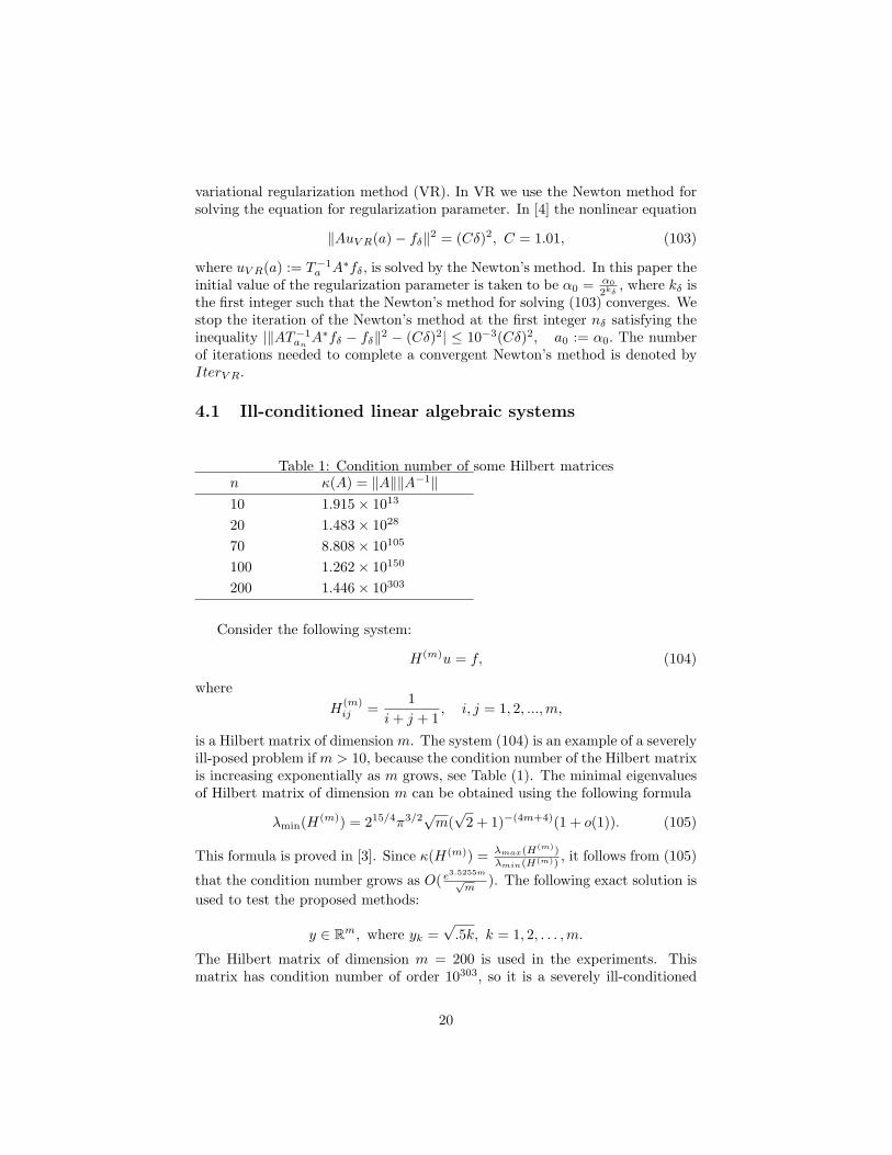
Table 1: Condition number of some Hilbert matricesn κ(A) = ‖A‖‖A−1‖10 1.915× 10¹³
20 1.483× 1028
70 8.808× 10105
100 1.262× 10150
200 1.446× 10303
Consider the following system:
H(m)u = f, (104)
whereH
(m)ij =
1i + j + 1
, i, j = 1, 2, ..., m,
is a Hilbert matrix of dimension m. The system (104) is an example of a severelyill-posed problem if m > 10, because the condition number of the Hilbert matrixis increasing exponentially as m grows, see Table (1). The minimal eigenvaluesof Hilbert matrix of dimension m can be obtained using the following formula
λmin(H(m)) = 215/4π3/2√
m(√
2 + 1)−(4m+4)(1 + o(1)). (105)
This formula is proved in [3]. Since κ(H(m)) = λmax(H(m))λmin(H(m))
, it follows from (105)
that the condition number grows as O( e3.5255m√m
). The following exact solution isused to test the proposed methods:
y ∈ Rm, where yk =√
.5k, k = 1, 2, . . . ,m.
The Hilbert matrix of dimension m = 200 is used in the experiments. Thismatrix has condition number of order 10303, so it is a severely ill-conditioned
20
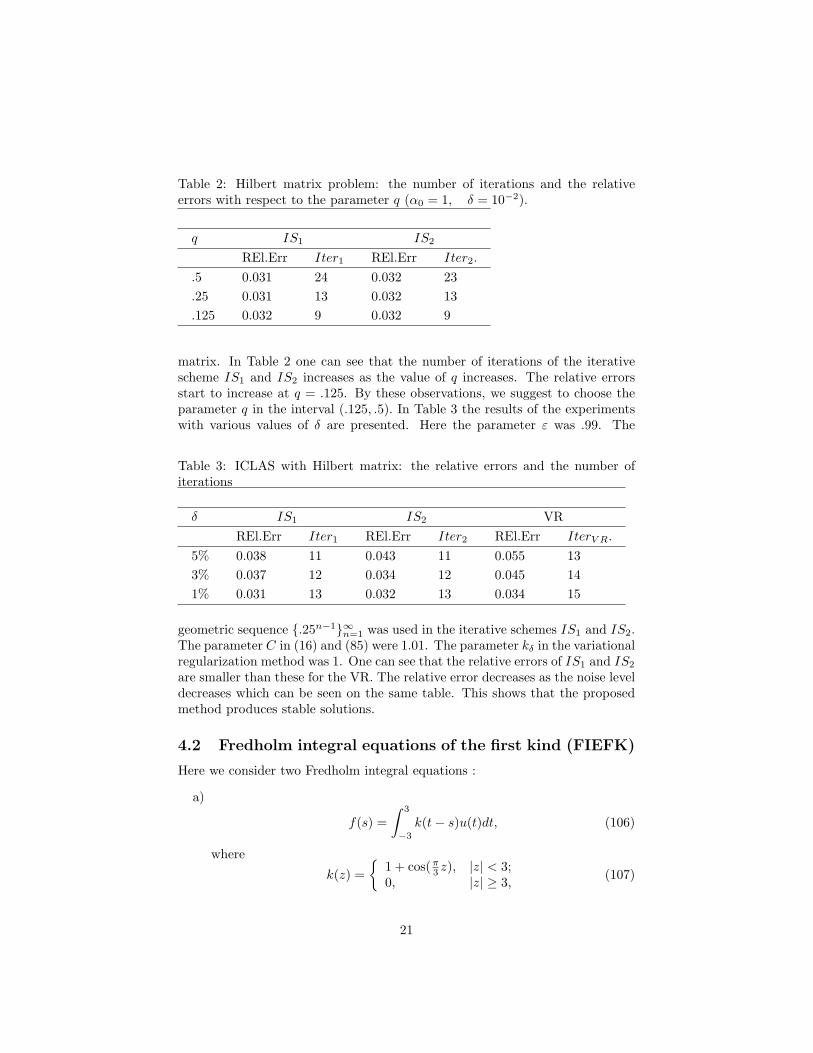
Table 2: Hilbert matrix problem: the number of iterations and the relativeerrors with respect to the parameter q (α0 = 1, δ = 10−2).
q IS1 IS2
REl.Err Iter1 REl.Err Iter2..5 0.031 24 0.032 23.25 0.031 13 0.032 13.125 0.032 9 0.032 9
matrix. In Table 2 one can see that the number of iterations of the iterativescheme IS1 and IS2 increases as the value of q increases. The relative errorsstart to increase at q = .125. By these observations, we suggest to choose theparameter q in the interval (.125, .5). In Table 3 the results of the experimentswith various values of δ are presented. Here the parameter ε was .99. The
Table 3: ICLAS with Hilbert matrix: the relative errors and the number ofiterations
δ IS1 IS2 VRREl.Err Iter1 REl.Err Iter2 REl.Err IterV R.
5% 0.038 11 0.043 11 0.055 133% 0.037 12 0.034 12 0.045 141% 0.031 13 0.032 13 0.034 15
geometric sequence {.25n−1}∞n=1 was used in the iterative schemes IS1 and IS2.The parameter C in (16) and (85) were 1.01. The parameter kδ in the variationalregularization method was 1. One can see that the relative errors of IS1 and IS2
are smaller than these for the VR. The relative error decreases as the noise leveldecreases which can be seen on the same table. This shows that the proposedmethod produces stable solutions.
4.2 Fredholm integral equations of the first kind (FIEFK)
Here we consider two Fredholm integral equations :
a)
f(s) =∫ 3
−3
k(t− s)u(t)dt, (106)
where
k(z) ={
1 + cos(π3 z), |z| < 3;
0, |z| ≥ 3, (107)
21
and
f(z) ={
(6 + z)[1− 1
2 cos(π3 z)
]− 92π sin(πz
3 ), |z| ≤ 6;0, |z| > 6. (108)
b)
f(s) =∫ 1
0
k(s, t)u(t)dt, s ∈ (0, 1), (109)
where
k(s, t) ={
s(t− 1), s < t;t(s− 1), s ≥ t, (110)
andf(s) = (s3 − s)/6. (111)
The problem a) is discussed in [5] where the solution to this problem is u(x) =k(x). The second problem is taken from [1] where the solution is u(x) = x. TheGalerkin’s method is used to discretized the integrals (106) and (109). For thebasis functions we use the following orthonormal box functions
φi(s) :=
{ √mc1
, [si−1, si] ;
0, otherwise,(112)
and
ψi(t) :=
{ √mc2
, [ti−1, ti] ;
0, otherwise,(113)
where si = d1 + id2m , ti = d3 + id4
m , i = 0, 1, 2, . . . , m. In the problem a) theparameters c1, c2, d1, d2, d3 and d4 are set to 12, 6, −6, 12, −3 and 6,respectively. In the second problem we use d1 = d3 = 0 and c1 = c2 = d2 =d4 = 1. Here we approximate the solution u(t) by u =
∑mj=1 cjψj(t). Therefore
solving problem (106) is reduced to solving the linear algebraic system
Ac = f, c, f ∈ Rm, (114)
where in problem a)
Aij =∫ 3
−3
∫ 6
−6
k(t− s)φi(s)ψj(t)dsdt
and fi =∫ 6
−6f(s)φi(s)ds, i, j = 1, 2, . . . , m, and in problem b)
Aij =∫ 1
0
∫ 1
0
k(s, t)φi(s)ψj(t)dsdt
and fi =∫ 1
0f(s)φi(s)ds, and cj = cj i, j = 1, 2, . . . , m.
The parameter m = 600 is used in problem a). In this case the conditionnumber of the matrix A with m = 600 is 3.427× 10⁹, so it is an ill-conditioned
22
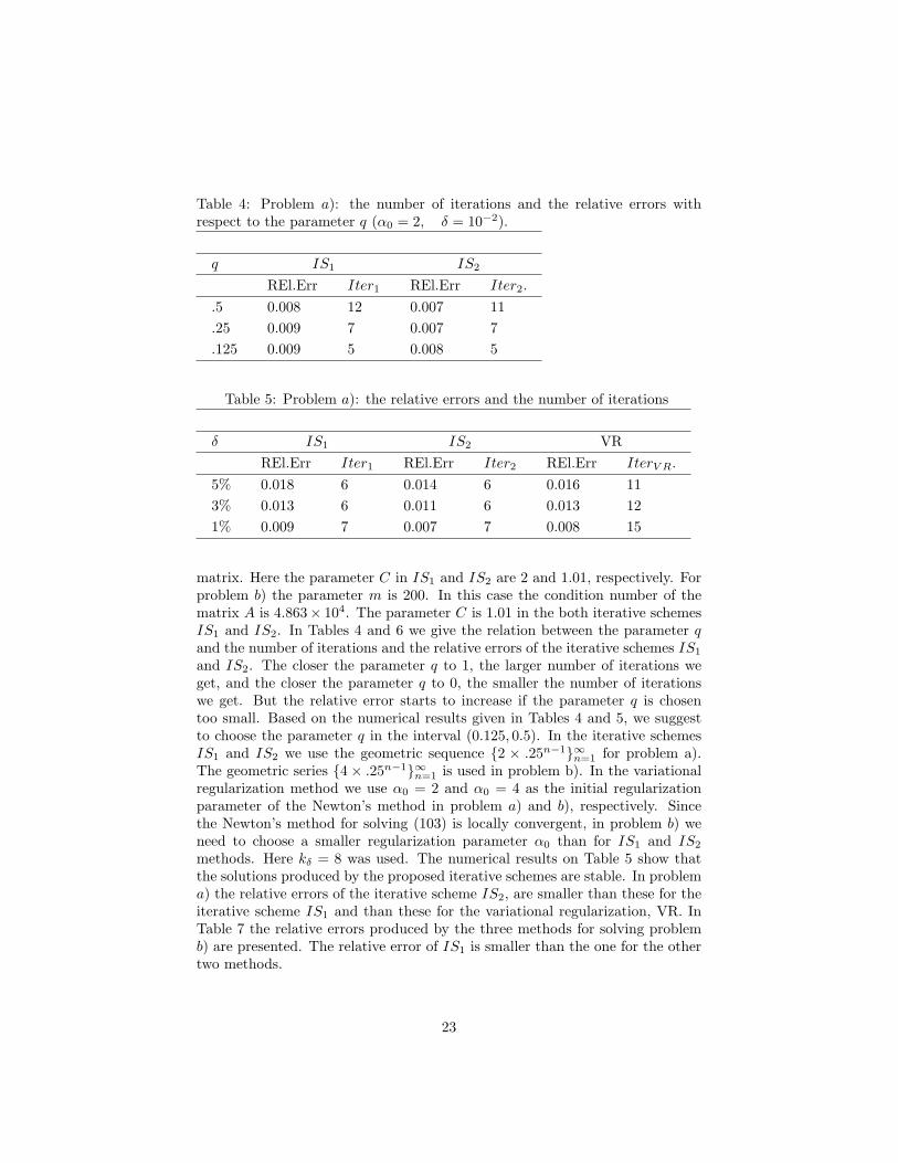
Table 4: Problem a): the number of iterations and the relative errors withrespect to the parameter q (α0 = 2, δ = 10−2).
q IS1 IS2
REl.Err Iter1 REl.Err Iter2..5 0.008 12 0.007 11.25 0.009 7 0.007 7.125 0.009 5 0.008 5
Table 5: Problem a): the relative errors and the number of iterations
δ IS1 IS2 VRREl.Err Iter1 REl.Err Iter2 REl.Err IterV R.
5% 0.018 6 0.014 6 0.016 113% 0.013 6 0.011 6 0.013 121% 0.009 7 0.007 7 0.008 15
matrix. Here the parameter C in IS1 and IS2 are 2 and 1.01, respectively. Forproblem b) the parameter m is 200. In this case the condition number of thematrix A is 4.863× 10⁴. The parameter C is 1.01 in the both iterative schemesIS1 and IS2. In Tables 4 and 6 we give the relation between the parameter qand the number of iterations and the relative errors of the iterative schemes IS1
and IS2. The closer the parameter q to 1, the larger number of iterations weget, and the closer the parameter q to 0, the smaller the number of iterationswe get. But the relative error starts to increase if the parameter q is chosentoo small. Based on the numerical results given in Tables 4 and 5, we suggestto choose the parameter q in the interval (0.125, 0.5). In the iterative schemesIS1 and IS2 we use the geometric sequence {2 × .25n−1}∞n=1 for problem a).The geometric series {4× .25n−1}∞n=1 is used in problem b). In the variationalregularization method we use α0 = 2 and α0 = 4 as the initial regularizationparameter of the Newton’s method in problem a) and b), respectively. Sincethe Newton’s method for solving (103) is locally convergent, in problem b) weneed to choose a smaller regularization parameter α0 than for IS1 and IS2
methods. Here kδ = 8 was used. The numerical results on Table 5 show thatthe solutions produced by the proposed iterative schemes are stable. In problema) the relative errors of the iterative scheme IS2, are smaller than these for theiterative scheme IS1 and than these for the variational regularization, VR. InTable 7 the relative errors produced by the three methods for solving problemb) are presented. The relative error of IS1 is smaller than the one for the othertwo methods.
23
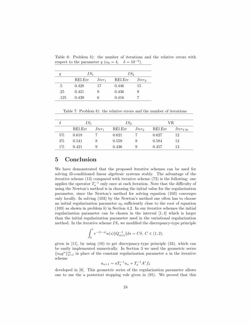
Table 6: Problem b): the number of iterations and the relative errors withrespect to the parameter q (α0 = 4, δ = 10−2).
q IS1 IS2
REl.Err Iter1 REl.Err Iter2..5 0.428 17 0.446 15.25 0.421 9 0.436 9.125 0.439 6 0.416 7
Table 7: Problem b): the relative errors and the number of iterations
δ IS1 IS2 VRREl.Err Iter1 REl.Err Iter2 REl.Err IterV R.
5% 0.618 7 0.621 7 0.627 123% 0.541 8 0.559 8 0.584 131% 0.421 9 0.436 9 0.457 13
5 Conclusion
We have demonstrated that the proposed iterative schemes can be used forsolving ill-conditioned linear algebraic systems stably. The advantage of theiterative scheme (13) compared with iterative scheme (72) is the following: oneapplies the operator T−1
a only once at each iteration. Note that the difficulty ofusing the Newton’s method is in choosing the initial value for the regularizationparameter, since the Newton’s method for solving equation (103) convergesonly locally. In solving (103) by the Newton’s method one often has to choosean initial regularization parameter a0 sufficiently close to the root of equation(103) as shown in problem b) in Section 4.2. In our iterative schemes the initialregularization parameter can be chosen in the interval [1, 4] which is largerthan the initial regularization parameter used in the variational regularizationmethod. In the iterative scheme IS1 we modified the discrepancy-type principle
∫ t
0
e−(t−s)a(s)‖Q−1a(s)‖ds = Cδ, C ∈ (1, 2),
given in [11], by using (10) to get discrepancy-type principle (33), which canbe easily implemented numerically. In Section 3 we used the geometric series{α0q
n}∞n=1 in place of the constant regularization parameter a in the iterativescheme
un+1 = aT−1a un + T−1
a A∗fδ
developed in [8]. This geometric series of the regularization parameter allowsone to use the a posteriori stopping rule given in (85). We proved that this
24
stopping rule produces stable approximation of the minimal norm solution ofequation (1). In all the experiments stopping rules (33) and (85) produce stableapproximations to the minimal norm solution of equation (1). It is of interest todevelop a method for choosing the parameter q in the proposed methods whichgives sufficiently small relative error and small number of iterations.
References
[1] Delves, L. M. and Mohamed, J. L., Computational Methods for IntegralEquations, Cambridge University Press, 1985; p. 310.
[2] Hoang, N.S. and Ramm, A. G. Solving ill-conditioned linear algebraic sys-tems by the dynamical systems method (DSM), Inverse Problems in Sci.and Engineering, 16, N5, (2008), 617-630.
[3] Kalyabin, G. A., An asymptotic formula for the minimal eigenvalues ofHilbert type matrices, Functional analysis and its applications, Vol. 35,No. 1, pp 67-70, 2001.
[4] Morozov, V., Methods of solving incorrectly posed problems, Springer Ver-lag, New York, 1984.
[5] Phillips, D. L., A technique for the numerical solution of certain integralequations of the first kind, J Assoc Comput Mach, 9, 84-97, 1962.
[6] Ramm, A. G., Inverse problems, Springer, New York, 2005.
[7] Ramm, A. G., Ill-posed problems with unbounded operators, Journ. Math.Anal. Appl., 325, , 490-495,2007.
[8] Ramm, A. G., Iterative solution of linear equations with unbounded oper-ators, Jour. Math. Anal. Appl., 330, N2, 1338-1346, 2007.
[9] Ramm, A. G., Dynamical systems method for solving operator equations,Elsevier, Amsterdam, 2007.
[10] Ramm, A. G., On unbounded operators and applications, Appl. Math.Lett., 21, 377-382, 2008.
[11] Ramm, A. G., Discrepancy principle for DSM, I, II, Comm. Nonlin. Sci.and Numer. Simulation, 10, N1, (2005), 95-101; 13, (2008), 1256-1263.
[12] Ramm, A. G., A new discrepancy principle, Journ. Math.Anal. Appl., 310,(2005), 342-345.
25


![Untitled-1 [] · 2020. 10. 9. · Thi Ill I Il Ill Olli Ill Ill 1 Ill ill Ill Il Ill ill Ill 11 Ill](https://img.pdfslide.us/doc/110x75/60d272307160da1c310a85a5/untitled-1-2020-10-9-thi-ill-i-il-ill-olli-ill-ill-1-ill-ill-ill-il-ill.jpg)