Embed Size (px)
Citation preview
Model Results Heuristics
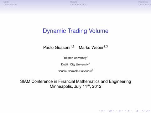
Dynamic Trading Volume
Paolo Guasoni1,2 Marko Weber2,3
Boston University1
Dublin City University2
Scuola Normale Superiore3
SIAM Conference in Financial Mathematics and EngineeringMinneapolis, July 11th, 2012
Model Results Heuristics
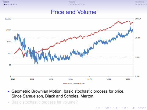
Price and Volume
• Geometric Brownian Motion: basic stochastic process for price.Since Samuelson, Black and Scholes, Merton.
• Basic stochastic process for volume?
Model Results Heuristics
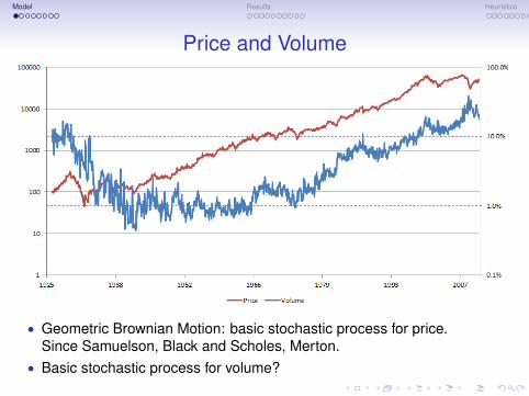
Price and Volume
• Geometric Brownian Motion: basic stochastic process for price.Since Samuelson, Black and Scholes, Merton.
• Basic stochastic process for volume?
Model Results Heuristics
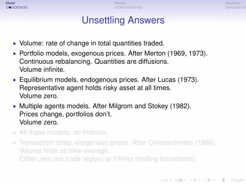
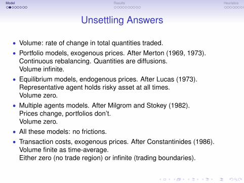
Unsettling Answers
• Volume: rate of change in total quantities traded.• Portfolio models, exogenous prices. After Merton (1969, 1973).
Continuous rebalancing. Quantities are diffusions.Volume infinite.
• Equilibrium models, endogenous prices. After Lucas (1973).Representative agent holds risky asset at all times.Volume zero.
• Multiple agents models. After Milgrom and Stokey (1982).Prices change, portfolios don’t.Volume zero.
• All these models: no frictions.• Transaction costs, exogenous prices. After Constantinides (1986).
Volume finite as time-average.Either zero (no trade region) or infinite (trading boundaries).

Model Results Heuristics
Unsettling Answers
• Volume: rate of change in total quantities traded.• Portfolio models, exogenous prices. After Merton (1969, 1973).
Continuous rebalancing. Quantities are diffusions.Volume infinite.
• Equilibrium models, endogenous prices. After Lucas (1973).Representative agent holds risky asset at all times.Volume zero.
• Multiple agents models. After Milgrom and Stokey (1982).Prices change, portfolios don’t.Volume zero.
• All these models: no frictions.• Transaction costs, exogenous prices. After Constantinides (1986).
Volume finite as time-average.Either zero (no trade region) or infinite (trading boundaries).

Model Results Heuristics
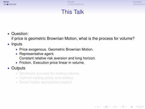
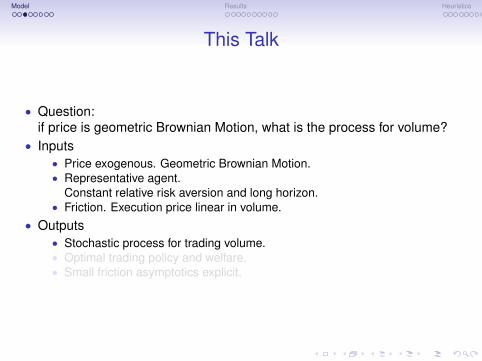
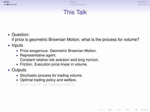
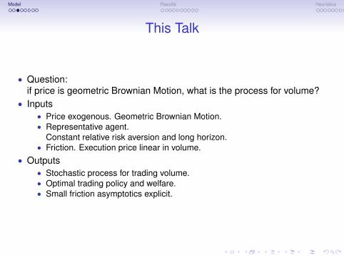
This Talk
• Question:if price is geometric Brownian Motion, what is the process for volume?
• Inputs• Price exogenous. Geometric Brownian Motion.• Representative agent.
Constant relative risk aversion and long horizon.• Friction. Execution price linear in volume.
• Outputs• Stochastic process for trading volume.• Optimal trading policy and welfare.• Small friction asymptotics explicit.

Model Results Heuristics
This Talk
• Question:if price is geometric Brownian Motion, what is the process for volume?
• Inputs• Price exogenous. Geometric Brownian Motion.• Representative agent.
Constant relative risk aversion and long horizon.• Friction. Execution price linear in volume.
• Outputs• Stochastic process for trading volume.• Optimal trading policy and welfare.• Small friction asymptotics explicit.
Model Results Heuristics
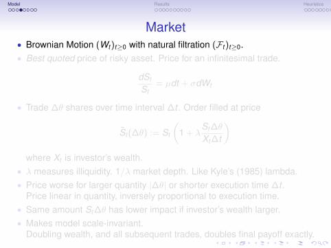
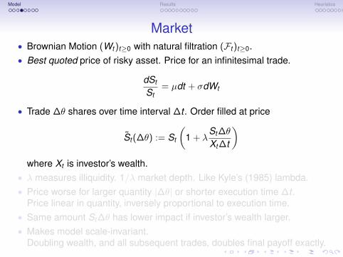
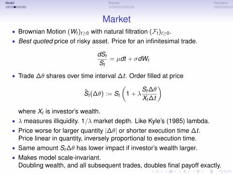
Market• Brownian Motion (Wt )t≥0 with natural filtration (Ft )t≥0.• Best quoted price of risky asset. Price for an infinitesimal trade.
dSt
St= µdt + σdWt
• Trade ∆θ shares over time interval ∆t . Order filled at price
St (∆θ) := St
(1 + λ
St ∆θ
Xt ∆t
)where Xt is investor’s wealth.
• λ measures illiquidity. 1/λ market depth. Like Kyle’s (1985) lambda.• Price worse for larger quantity |∆θ| or shorter execution time ∆t .
Price linear in quantity, inversely proportional to execution time.• Same amount St ∆θ has lower impact if investor’s wealth larger.• Makes model scale-invariant.
Doubling wealth, and all subsequent trades, doubles final payoff exactly.

Model Results Heuristics
Market• Brownian Motion (Wt )t≥0 with natural filtration (Ft )t≥0.• Best quoted price of risky asset. Price for an infinitesimal trade.
dSt
St= µdt + σdWt
• Trade ∆θ shares over time interval ∆t . Order filled at price
St (∆θ) := St
(1 + λ
St ∆θ
Xt ∆t
)where Xt is investor’s wealth.
• λ measures illiquidity. 1/λ market depth. Like Kyle’s (1985) lambda.• Price worse for larger quantity |∆θ| or shorter execution time ∆t .
Price linear in quantity, inversely proportional to execution time.• Same amount St ∆θ has lower impact if investor’s wealth larger.• Makes model scale-invariant.
Doubling wealth, and all subsequent trades, doubles final payoff exactly.
Model Results Heuristics
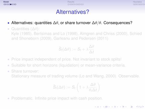
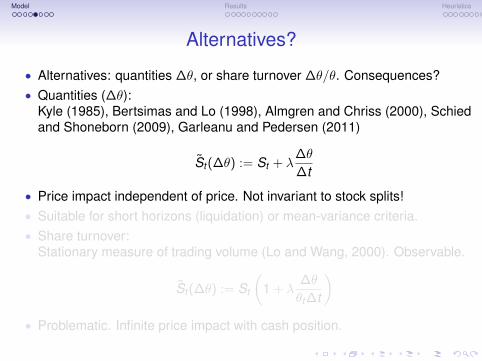
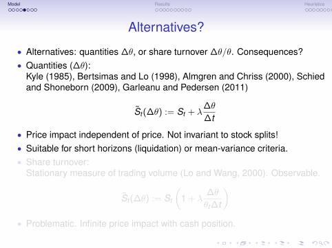
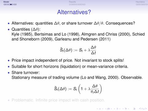
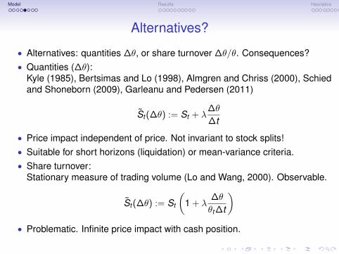
Alternatives?
• Alternatives: quantities ∆θ, or share turnover ∆θ/θ. Consequences?• Quantities (∆θ):
Kyle (1985), Bertsimas and Lo (1998), Almgren and Chriss (2000), Schiedand Shoneborn (2009), Garleanu and Pedersen (2011)
St (∆θ) := St + λ∆θ
∆t
• Price impact independent of price. Not invariant to stock splits!• Suitable for short horizons (liquidation) or mean-variance criteria.• Share turnover:
Stationary measure of trading volume (Lo and Wang, 2000). Observable.
St (∆θ) := St
(1 + λ
∆θ
θt ∆t
)• Problematic. Infinite price impact with cash position.

Model Results Heuristics
Alternatives?
• Alternatives: quantities ∆θ, or share turnover ∆θ/θ. Consequences?• Quantities (∆θ):
Kyle (1985), Bertsimas and Lo (1998), Almgren and Chriss (2000), Schiedand Shoneborn (2009), Garleanu and Pedersen (2011)
St (∆θ) := St + λ∆θ
∆t
• Price impact independent of price. Not invariant to stock splits!• Suitable for short horizons (liquidation) or mean-variance criteria.• Share turnover:
Stationary measure of trading volume (Lo and Wang, 2000). Observable.
St (∆θ) := St
(1 + λ
∆θ
θt ∆t
)• Problematic. Infinite price impact with cash position.
Model Results Heuristics
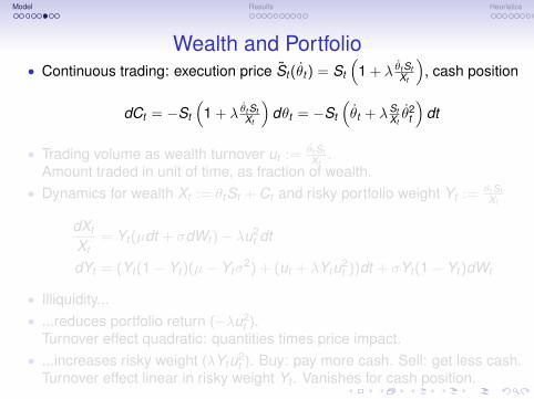
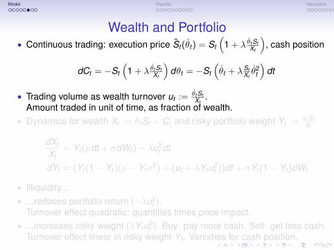
Wealth and Portfolio• Continuous trading: execution price St (θt ) = St
(1 + λ θt St
Xt
), cash position
dCt = −St
(1 + λ θt St
Xt
)dθt = −St
(θt + λSt
Xtθ2
t
)dt
• Trading volume as wealth turnover ut := θt StXt
.Amount traded in unit of time, as fraction of wealth.
• Dynamics for wealth Xt := θtSt + Ct and risky portfolio weight Yt := θt StXt
dXt
Xt= Yt (µdt + σdWt )− λu2
t dt
dYt = (Yt (1− Yt )(µ− Ytσ2) + (ut + λYtu2
t ))dt + σYt (1− Yt )dWt
• Illiquidity...• ...reduces portfolio return (−λu2
t ).Turnover effect quadratic: quantities times price impact.
• ...increases risky weight (λYtu2t ). Buy: pay more cash. Sell: get less cash.
Turnover effect linear in risky weight Yt . Vanishes for cash position.
Model Results Heuristics
Admissible Strategies
DefinitionAdmissible strategy: process (ut )t≥0, adapted to Ft , such that system
dXt
Xt= Yt (µdt + σdWt )− λu2
t dt
dYt = (Yt (1− Yt )(µ− Ytσ2) + (ut + λYtu2
t ))dt + σYt (1− Yt )dWt
has unique solution satisfying Xt ≥ 0 a.s. for all t ≥ 0.
• Contrast to models without frictions or with transaction costs:control variable is not risky weight Yt , but its “rate of change” ut .
• Portfolio weight Yt is now a state variable.• Illiquid vs. perfectly liquid market.
Steering a ship vs. driving a race car.• Frictionless solution Yt = µ
γσ2 unfeasible. A still ship in stormy sea.
Model Results Heuristics
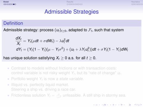
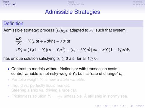
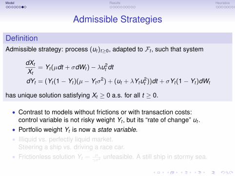
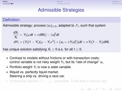
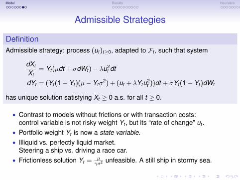
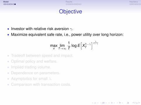
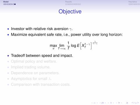
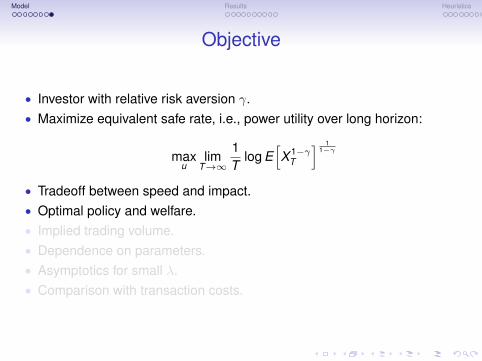
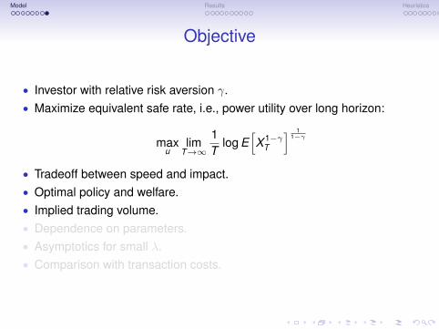
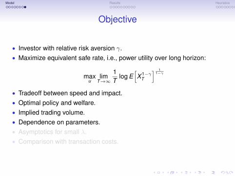
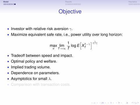
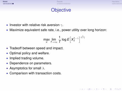
Objective
• Investor with relative risk aversion γ.• Maximize equivalent safe rate, i.e., power utility over long horizon:
maxu
limT→∞
1T
log E[X 1−γ
T
] 11−γ
• Tradeoff between speed and impact.• Optimal policy and welfare.• Implied trading volume.• Dependence on parameters.• Asymptotics for small λ.• Comparison with transaction costs.
Model Results Heuristics
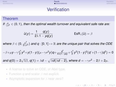
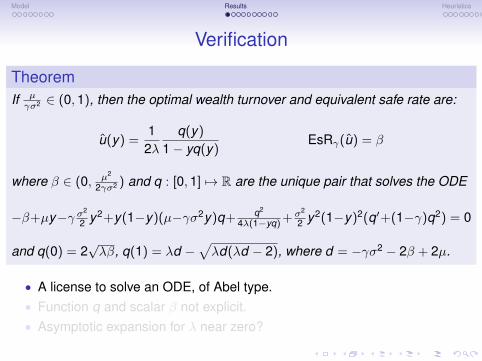
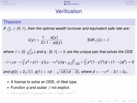
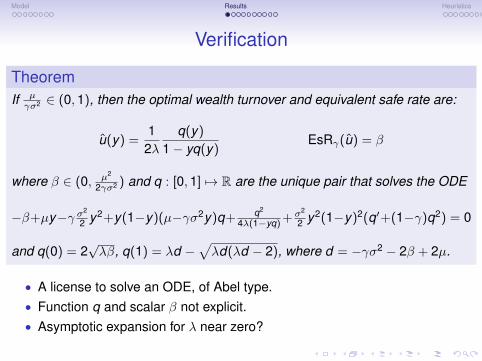
Verification
TheoremIf µγσ2 ∈ (0,1), then the optimal wealth turnover and equivalent safe rate are:
u(y) =1
2λq(y)
1− yq(y)EsRγ(u) = β
where β ∈ (0, µ2
2γσ2 ) and q : [0,1] 7→ R are the unique pair that solves the ODE
−β+µy−γ σ2
2 y2+y(1−y)(µ−γσ2y)q+ q2
4λ(1−yq) + σ2
2 y2(1−y)2(q′+(1−γ)q2) = 0
and q(0) = 2√λβ, q(1) = λd −
√λd(λd − 2), where d = −γσ2 − 2β + 2µ.
• A license to solve an ODE, of Abel type.• Function q and scalar β not explicit.• Asymptotic expansion for λ near zero?
Model Results Heuristics
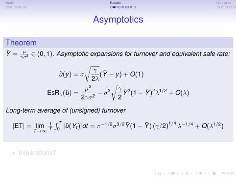
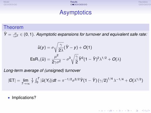
Asymptotics
TheoremY = µ
γσ2 ∈ (0,1). Asymptotic expansions for turnover and equivalent safe rate:
u(y) = σ
√γ
2λ(Y − y) + O(1)
EsRγ(u) =µ2
2γσ2 − σ3√γ
2Y 2(1− Y )2λ1/2 + O(λ)
Long-term average of (unsigned) turnover
|ET| = limT→∞
1T
∫ T0 |u(Yt )|dt = π−1/2σ3/2Y (1− Y ) (γ/2)1/4
λ−1/4 + O(λ1/2)
• Implications?
Model Results Heuristics
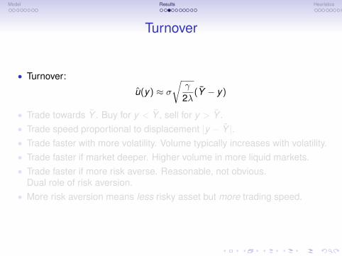
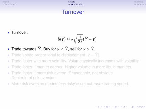
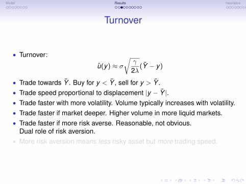
Turnover
• Turnover:
u(y) ≈ σ√
γ
2λ(Y − y)
• Trade towards Y . Buy for y < Y , sell for y > Y .• Trade speed proportional to displacement |y − Y |.• Trade faster with more volatility. Volume typically increases with volatility.• Trade faster if market deeper. Higher volume in more liquid markets.• Trade faster if more risk averse. Reasonable, not obvious.
Dual role of risk aversion.• More risk aversion means less risky asset but more trading speed.
Model Results Heuristics
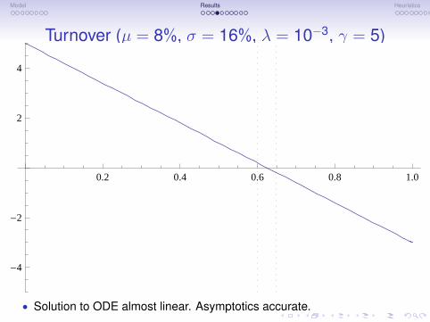
Turnover (µ = 8%, σ = 16%, λ = 10−3, γ = 5)
0.2 0.4 0.6 0.8 1.0
-4
-2
2
4
• Solution to ODE almost linear. Asymptotics accurate.
Model Results Heuristics
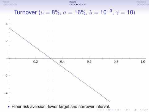
Turnover (µ = 8%, σ = 16%, λ = 10−3, γ = 10)
0.2 0.4 0.6 0.8 1.0
-4
-2
2
4
• Hiher risk aversion: lower target and narrower interval.
Model Results Heuristics
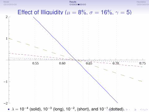
Effect of Illiquidity (µ = 8%, σ = 16%, γ = 5)
0.55 0.60 0.65 0.70 0.75
-2
-1
1
2
• λ = 10−4 (solid), 10−3 (long), 10−2, (short), and 10−1 (dotted).
Model Results Heuristics
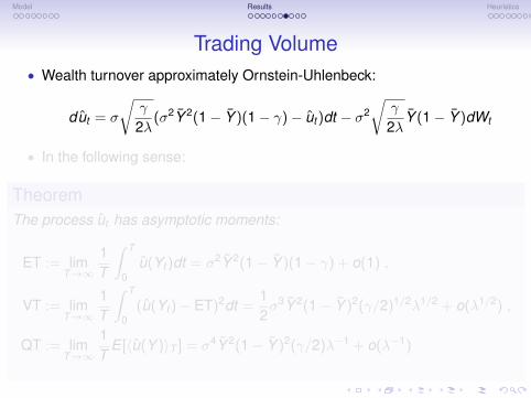
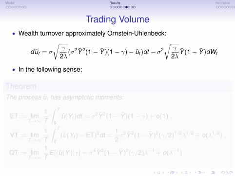
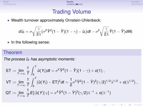
Trading Volume• Wealth turnover approximately Ornstein-Uhlenbeck:
dut = σ
√γ
2λ(σ2Y 2(1− Y )(1− γ)− ut )dt − σ2
√γ
2λY (1− Y )dWt
• In the following sense:
TheoremThe process ut has asymptotic moments:
ET := limT→∞
1T
∫ T
0u(Yt )dt = σ2Y 2(1− Y )(1− γ) + o(1) ,
VT := limT→∞
1T
∫ T
0(u(Yt )− ET)2dt =
12σ3Y 2(1− Y )2(γ/2)1/2λ1/2 + o(λ1/2) ,
QT := limT→∞
1T
E [〈u(Y )〉T ] = σ4Y 2(1− Y )2(γ/2)λ−1 + o(λ−1)
Model Results Heuristics
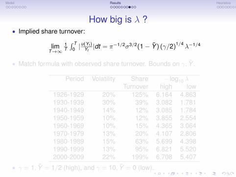
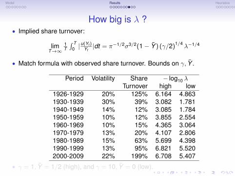
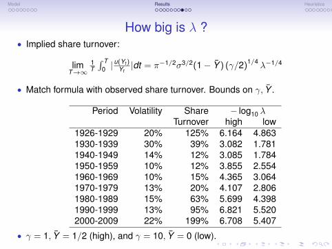
How big is λ ?• Implied share turnover:
limT→∞
1T
∫ T0 |
u(Yt )Yt|dt = π−1/2σ3/2(1− Y ) (γ/2)1/4
λ−1/4
• Match formula with observed share turnover. Bounds on γ, Y .
Period Volatility Share − log10 λTurnover high low
1926-1929 20% 125% 6.164 4.8631930-1939 30% 39% 3.082 1.7811940-1949 14% 12% 3.085 1.7841950-1959 10% 12% 3.855 2.5541960-1969 10% 15% 4.365 3.0641970-1979 13% 20% 4.107 2.8061980-1989 15% 63% 5.699 4.3981990-1999 13% 95% 6.821 5.5202000-2009 22% 199% 6.708 5.407
• γ = 1, Y = 1/2 (high), and γ = 10, Y = 0 (low).
Model Results Heuristics
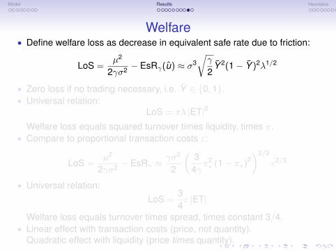
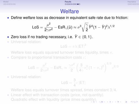
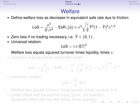
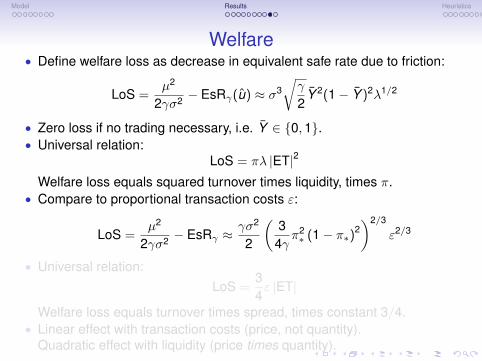
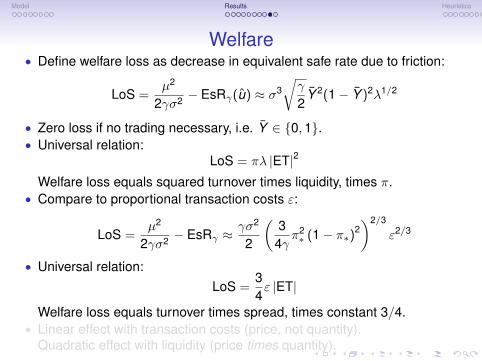
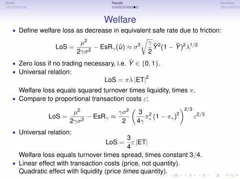
Welfare• Define welfare loss as decrease in equivalent safe rate due to friction:
LoS =µ2
2γσ2 − EsRγ(u) ≈ σ3√γ
2Y 2(1− Y )2λ1/2
• Zero loss if no trading necessary, i.e. Y ∈ {0,1}.• Universal relation:
LoS = πλ |ET|2
Welfare loss equals squared turnover times liquidity, times π.• Compare to proportional transaction costs ε:
LoS =µ2
2γσ2 − EsRγ ≈γσ2
2
(3
4γπ2∗ (1− π∗)2
)2/3
ε2/3
• Universal relation:LoS =
34ε |ET|
Welfare loss equals turnover times spread, times constant 3/4.• Linear effect with transaction costs (price, not quantity).
Quadratic effect with liquidity (price times quantity).
Model Results Heuristics
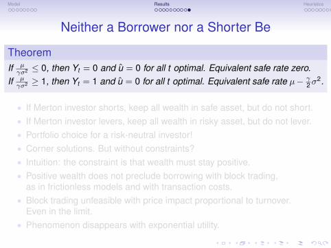
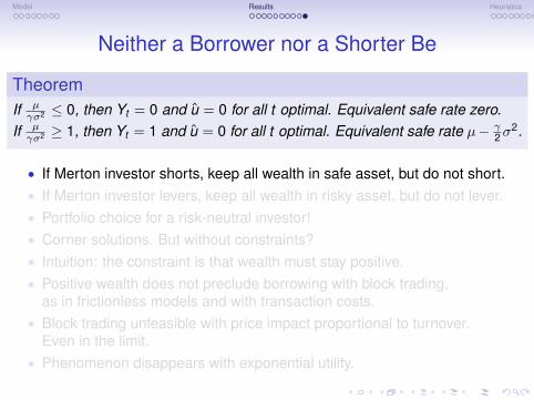
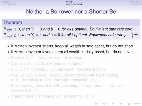
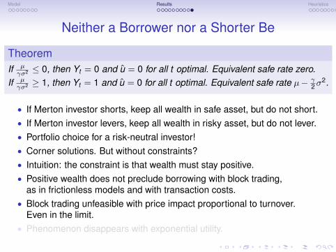
Neither a Borrower nor a Shorter Be
TheoremIf µγσ2 ≤ 0, then Yt = 0 and u = 0 for all t optimal. Equivalent safe rate zero.
If µγσ2 ≥ 1, then Yt = 1 and u = 0 for all t optimal. Equivalent safe rate µ− γ
2σ2.
• If Merton investor shorts, keep all wealth in safe asset, but do not short.• If Merton investor levers, keep all wealth in risky asset, but do not lever.• Portfolio choice for a risk-neutral investor!• Corner solutions. But without constraints?• Intuition: the constraint is that wealth must stay positive.• Positive wealth does not preclude borrowing with block trading,
as in frictionless models and with transaction costs.• Block trading unfeasible with price impact proportional to turnover.
Even in the limit.• Phenomenon disappears with exponential utility.
Model Results Heuristics
Neither a Borrower nor a Shorter Be
TheoremIf µγσ2 ≤ 0, then Yt = 0 and u = 0 for all t optimal. Equivalent safe rate zero.
If µγσ2 ≥ 1, then Yt = 1 and u = 0 for all t optimal. Equivalent safe rate µ− γ
2σ2.
• If Merton investor shorts, keep all wealth in safe asset, but do not short.• If Merton investor levers, keep all wealth in risky asset, but do not lever.• Portfolio choice for a risk-neutral investor!• Corner solutions. But without constraints?• Intuition: the constraint is that wealth must stay positive.• Positive wealth does not preclude borrowing with block trading,
as in frictionless models and with transaction costs.• Block trading unfeasible with price impact proportional to turnover.
Even in the limit.• Phenomenon disappears with exponential utility.
Model Results Heuristics
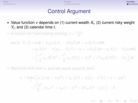
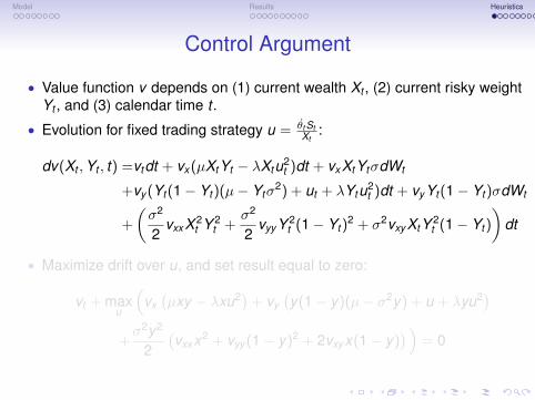
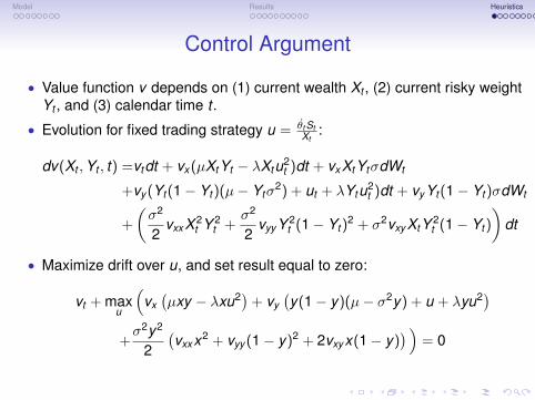
Control Argument
• Value function v depends on (1) current wealth Xt , (2) current risky weightYt , and (3) calendar time t .
• Evolution for fixed trading strategy u = θt StXt
:
dv(Xt ,Yt , t) =vtdt + vx (µXtYt − λXtu2t )dt + vxXtYtσdWt
+vy (Yt (1− Yt )(µ− Ytσ2) + ut + λYtu2
t )dt + vy Yt (1− Yt )σdWt
+
(σ2
2vxxX 2
t Y 2t +
σ2
2vyy Y 2
t (1− Yt )2 + σ2vxy XtY 2
t (1− Yt )
)dt
• Maximize drift over u, and set result equal to zero:
vt + maxu
(vx(µxy − λxu2)+ vy
(y(1− y)(µ− σ2y) + u + λyu2)
+σ2y2
2(vxxx2 + vyy (1− y)2 + 2vxy x(1− y)
) )= 0
Model Results Heuristics
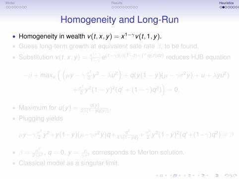
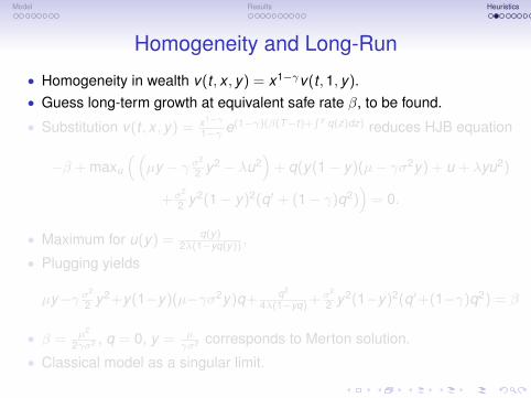
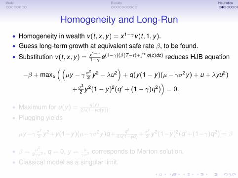
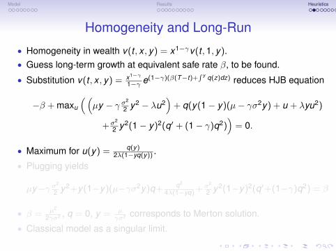
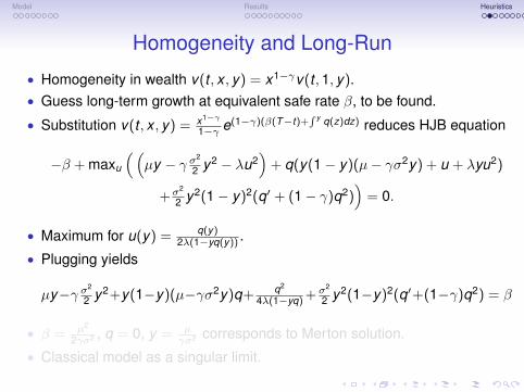
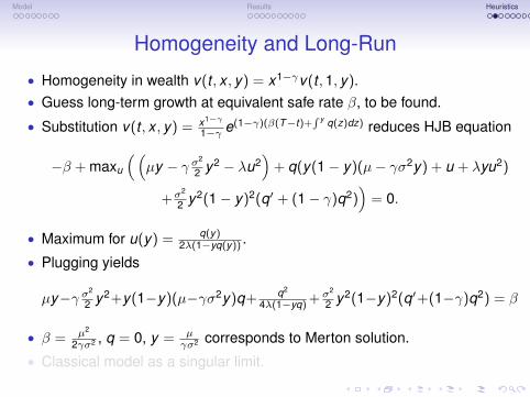
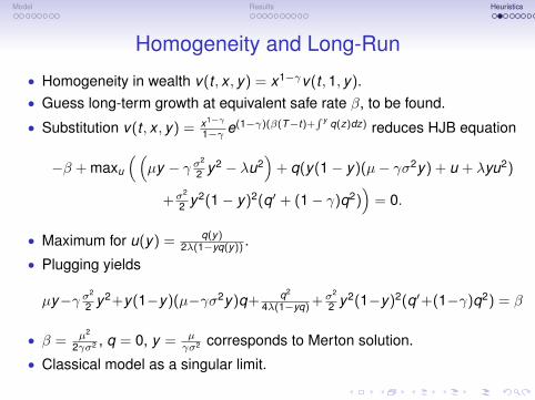
Homogeneity and Long-Run
• Homogeneity in wealth v(t , x , y) = x1−γv(t ,1, y).• Guess long-term growth at equivalent safe rate β, to be found.
• Substitution v(t , x , y) = x1−γ
1−γ e(1−γ)(β(T−t)+∫ y q(z)dz) reduces HJB equation
−β + maxu
((µy − γ σ
2
2 y2 − λu2)
+ q(y(1− y)(µ− γσ2y) + u + λyu2)
+σ2
2 y2(1− y)2(q′ + (1− γ)q2))
= 0.
• Maximum for u(y) = q(y)2λ(1−yq(y)) .
• Plugging yields
µy−γ σ2
2 y2+y(1−y)(µ−γσ2y)q+ q2
4λ(1−yq) + σ2
2 y2(1−y)2(q′+(1−γ)q2) = β
• β = µ2
2γσ2 , q = 0, y = µγσ2 corresponds to Merton solution.
• Classical model as a singular limit.
Model Results Heuristics
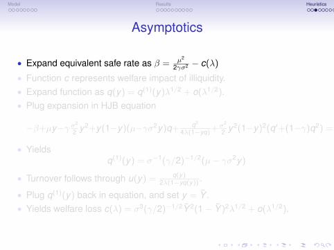
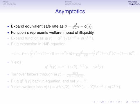
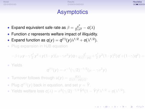
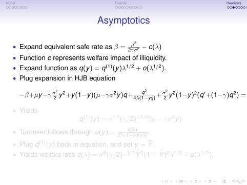
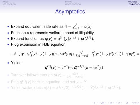
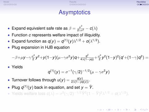
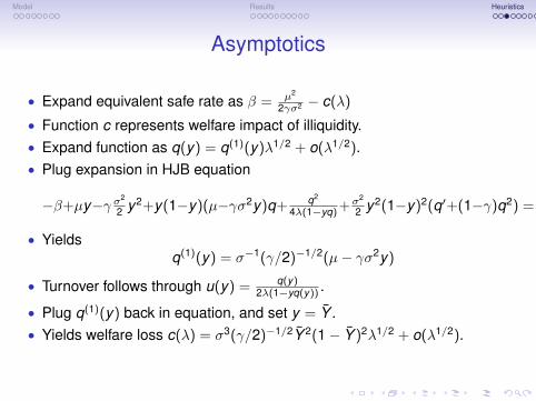
Asymptotics
• Expand equivalent safe rate as β = µ2
2γσ2 − c(λ)
• Function c represents welfare impact of illiquidity.• Expand function as q(y) = q(1)(y)λ1/2 + o(λ1/2).• Plug expansion in HJB equation
−β+µy−γ σ2
2 y2+y(1−y)(µ−γσ2y)q+ q2
4λ(1−yq) +σ2
2 y2(1−y)2(q′+(1−γ)q2) = 0
• Yieldsq(1)(y) = σ−1(γ/2)−1/2(µ− γσ2y)
• Turnover follows through u(y) = q(y)2λ(1−yq(y)) .
• Plug q(1)(y) back in equation, and set y = Y .• Yields welfare loss c(λ) = σ3(γ/2)−1/2Y 2(1− Y )2λ1/2 + o(λ1/2).
Model Results Heuristics
Asymptotics
• Expand equivalent safe rate as β = µ2
2γσ2 − c(λ)
• Function c represents welfare impact of illiquidity.• Expand function as q(y) = q(1)(y)λ1/2 + o(λ1/2).• Plug expansion in HJB equation
−β+µy−γ σ2
2 y2+y(1−y)(µ−γσ2y)q+ q2
4λ(1−yq) +σ2
2 y2(1−y)2(q′+(1−γ)q2) = 0
• Yieldsq(1)(y) = σ−1(γ/2)−1/2(µ− γσ2y)
• Turnover follows through u(y) = q(y)2λ(1−yq(y)) .
• Plug q(1)(y) back in equation, and set y = Y .• Yields welfare loss c(λ) = σ3(γ/2)−1/2Y 2(1− Y )2λ1/2 + o(λ1/2).
Model Results Heuristics
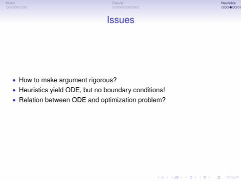
Issues
• How to make argument rigorous?• Heuristics yield ODE, but no boundary conditions!• Relation between ODE and optimization problem?
Model Results Heuristics
Issues
• How to make argument rigorous?• Heuristics yield ODE, but no boundary conditions!• Relation between ODE and optimization problem?
Model Results Heuristics
Issues
• How to make argument rigorous?• Heuristics yield ODE, but no boundary conditions!• Relation between ODE and optimization problem?
Model Results Heuristics
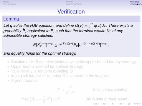
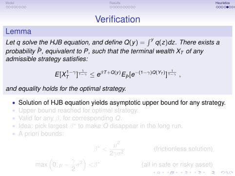
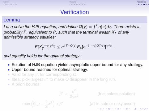
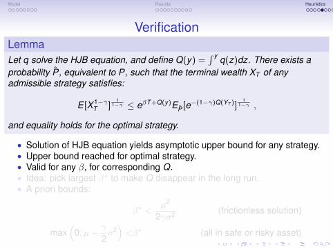
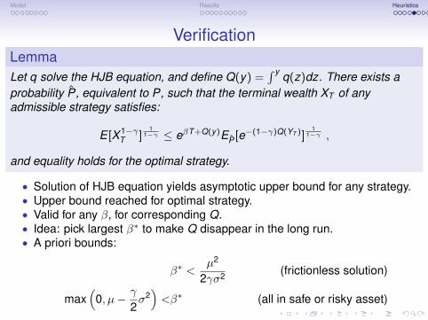
VerificationLemmaLet q solve the HJB equation, and define Q(y) =
∫ y q(z)dz. There exists aprobability P, equivalent to P, such that the terminal wealth XT of anyadmissible strategy satisfies:
E [X 1−γT ]
11−γ ≤ eβT +Q(y)EP [e−(1−γ)Q(YT )]
11−γ ,
and equality holds for the optimal strategy.
• Solution of HJB equation yields asymptotic upper bound for any strategy.• Upper bound reached for optimal strategy.• Valid for any β, for corresponding Q.• Idea: pick largest β∗ to make Q disappear in the long run.• A priori bounds:
β∗ <µ2
2γσ2 (frictionless solution)
max(
0, µ− γ
2σ2)<β∗ (all in safe or risky asset)
Model Results Heuristics
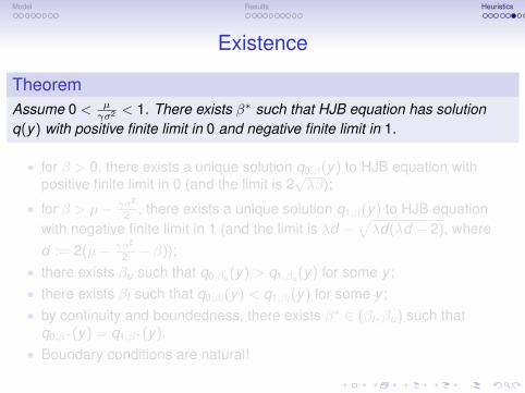
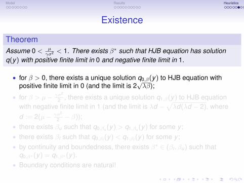
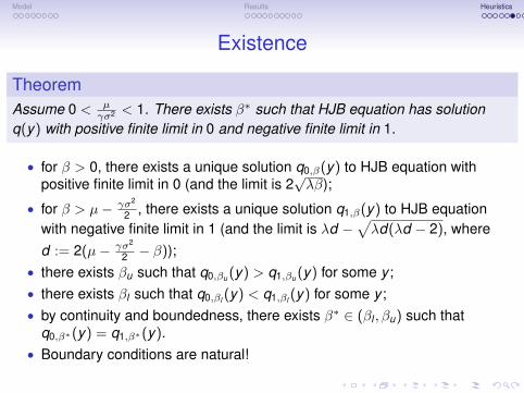
Existence
TheoremAssume 0 < µ
γσ2 < 1. There exists β∗ such that HJB equation has solutionq(y) with positive finite limit in 0 and negative finite limit in 1.
• for β > 0, there exists a unique solution q0,β(y) to HJB equation withpositive finite limit in 0 (and the limit is 2
√λβ);
• for β > µ− γσ2
2 , there exists a unique solution q1,β(y) to HJB equationwith negative finite limit in 1 (and the limit is λd −
√λd(λd − 2), where
d := 2(µ− γσ2
2 − β));• there exists βu such that q0,βu (y) > q1,βu (y) for some y ;• there exists βl such that q0,βl (y) < q1,βl (y) for some y ;• by continuity and boundedness, there exists β∗ ∈ (βl , βu) such that
q0,β∗(y) = q1,β∗(y).• Boundary conditions are natural!
Model Results Heuristics
Existence
TheoremAssume 0 < µ
γσ2 < 1. There exists β∗ such that HJB equation has solutionq(y) with positive finite limit in 0 and negative finite limit in 1.
• for β > 0, there exists a unique solution q0,β(y) to HJB equation withpositive finite limit in 0 (and the limit is 2
√λβ);
• for β > µ− γσ2
2 , there exists a unique solution q1,β(y) to HJB equationwith negative finite limit in 1 (and the limit is λd −
√λd(λd − 2), where
d := 2(µ− γσ2
2 − β));• there exists βu such that q0,βu (y) > q1,βu (y) for some y ;• there exists βl such that q0,βl (y) < q1,βl (y) for some y ;• by continuity and boundedness, there exists β∗ ∈ (βl , βu) such that
q0,β∗(y) = q1,β∗(y).• Boundary conditions are natural!
Model Results Heuristics
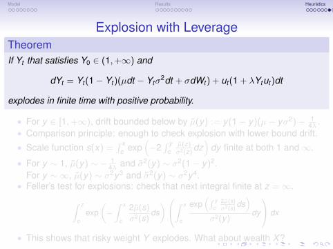
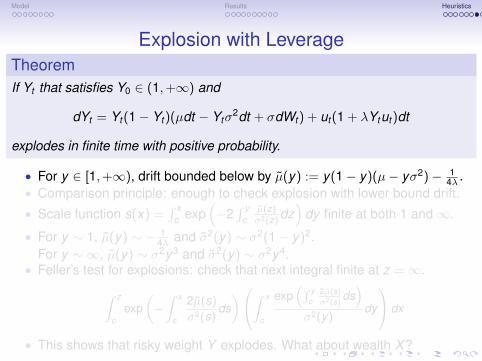
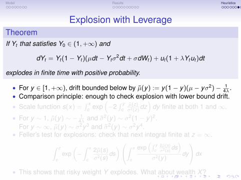
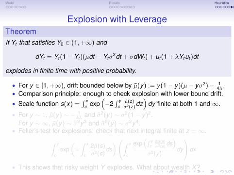
Explosion with LeverageTheoremIf Yt that satisfies Y0 ∈ (1,+∞) and
dYt = Yt (1− Yt )(µdt − Ytσ2dt + σdWt ) + ut (1 + λYtut )dt
explodes in finite time with positive probability.
• For y ∈ [1,+∞), drift bounded below by µ(y) := y(1− y)(µ− yσ2)− 14λ .
• Comparison principle: enough to check explosion with lower bound drift.• Scale function s(x) =
∫ xc exp
(−2∫ y
cµ(z)σ2(z)
dz)
dy finite at both 1 and∞.
• For y ∼ 1, µ(y) ∼ − 14λ and σ2(y) ∼ σ2(1− y)2.
For y ∼ ∞, µ(y) ∼ σ2y3 and σ2(y) ∼ σ2y4.• Feller’s test for explosions: check that next integral finite at z =∞.∫ z
cexp
(−∫ x
c
2µ(s)σ2(s)
ds)∫ x
c
exp(∫ y
c2µ(s)
σ2(s)ds)
σ2(y)dy
dx
• This shows that risky weight Y explodes. What about wealth X?
Model Results Heuristics
Explosion with LeverageTheoremIf Yt that satisfies Y0 ∈ (1,+∞) and
dYt = Yt (1− Yt )(µdt − Ytσ2dt + σdWt ) + ut (1 + λYtut )dt
explodes in finite time with positive probability.
• For y ∈ [1,+∞), drift bounded below by µ(y) := y(1− y)(µ− yσ2)− 14λ .
• Comparison principle: enough to check explosion with lower bound drift.• Scale function s(x) =
∫ xc exp
(−2∫ y
cµ(z)σ2(z)
dz)
dy finite at both 1 and∞.
• For y ∼ 1, µ(y) ∼ − 14λ and σ2(y) ∼ σ2(1− y)2.
For y ∼ ∞, µ(y) ∼ σ2y3 and σ2(y) ∼ σ2y4.• Feller’s test for explosions: check that next integral finite at z =∞.∫ z
cexp
(−∫ x
c
2µ(s)σ2(s)
ds)∫ x
c
exp(∫ y
c2µ(s)
σ2(s)ds)
σ2(y)dy
dx
• This shows that risky weight Y explodes. What about wealth X?
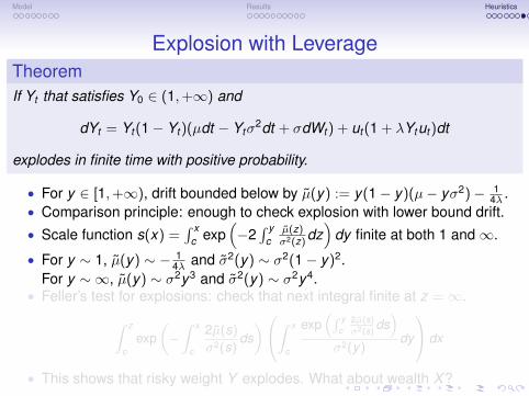
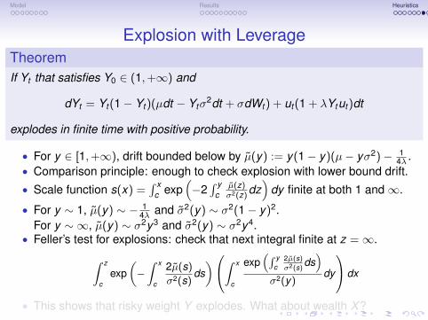
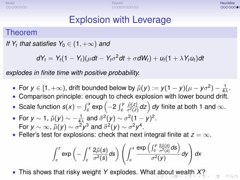
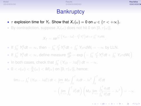
Model Results Heuristics
Bankruptcy
• τ explosion time for Yt . Show that Xτ (ω) = 0 on ω ∈ {τ < +∞}.• By contradiction, suppose Xt (ω) does not hit 0 on [0, τ(ω)].
XT = xe∫ T
0
(Ytµ−λu2
t −σ22 Y 2
t
)dt+σ
∫ T0 Yt dWt .
• If∫ τ
0 Y 2t dt =∞, then −
∫ τ0σ2
2 Y 2t dt +
∫ τ0 YtσdWt = −∞ by LLN.
• If∫ τ
0 Y 2t dt <∞, define measure dP
dP = exp(−∫ τ
0σ2
2 Y 2t dt +
∫ τ0 YtσdWt
)• In both cases, check that
∫ τ0
(Ytµ− λu2
t)
dt = −∞.
• 0 < ε(ω) < StXt
(ω) < M(ω) on [0, τ(ω)], hence:
limT→τ
∫ T0
(Ytµ− λu2
t)
dt < limT→τ
Mµ
∫ T
0θtdt − λε2
∫ T
0θ2
t dt
=
(lim
T→τ
∫ T
0θ2
t dt)(
Mµ limT→τ
∫ T0 θtdt∫ T0 θ2
t dt− λε2
)= −∞.
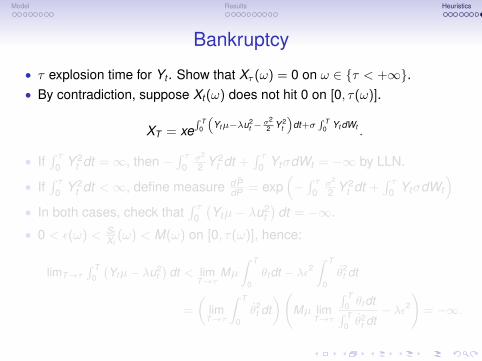
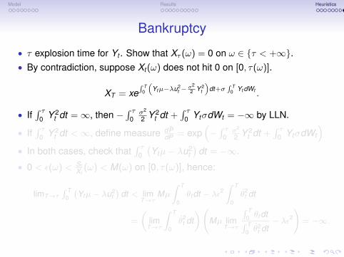
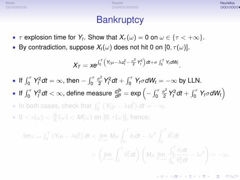
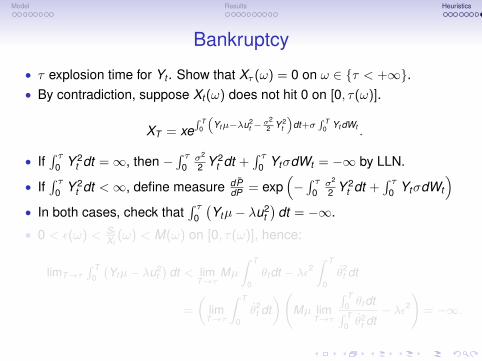
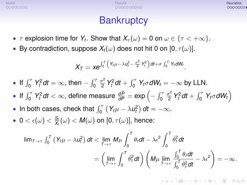
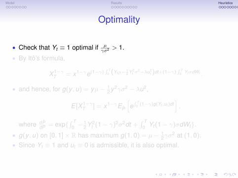
Model Results Heuristics
Optimality
• Check that Yt ≡ 1 optimal if µγσ2 > 1.
• By Itô’s formula,
X 1−γT = x1−γe(1−γ)
∫ T0 (Ytµ− 1
2 Y 2t σ
2−λu2t )dt+(1−γ)
∫ T0 YtσdWt .
• and hence, for g(y ,u) = yµ− 12 y2γσ2 − λu2,
E [X 1−γT ] = x1−γEP
[e∫ T
0 (1−γ)g(Yt ,ut )dt],
where dPdP = exp{
∫ T0 −
12 Y 2
t (1− γ)2σ2dt +∫ T
0 Yt (1− γ)σdWt}.• g(y ,u) on [0,1]× R has maximum g(1,0) = µ− 1
2γσ2 at (1,0).
• Since Yt ≡ 1 and ut ≡ 0 is admissible, it is also optimal.
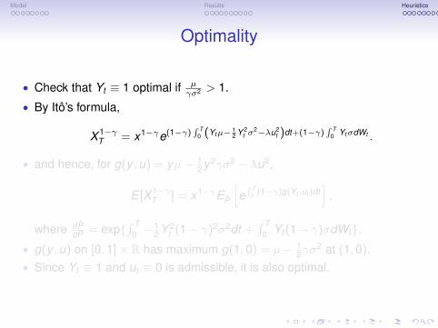
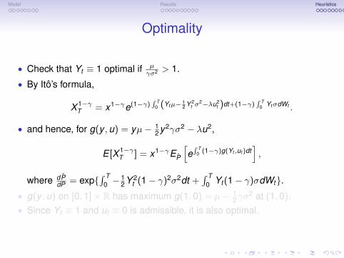
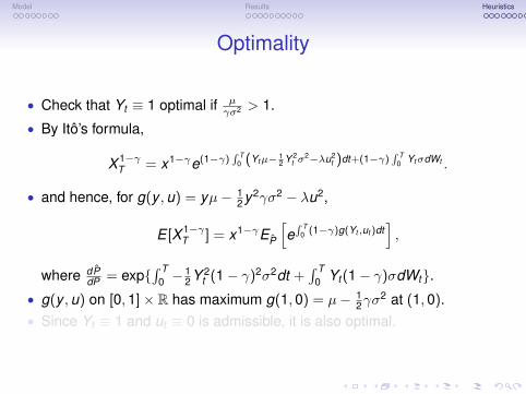
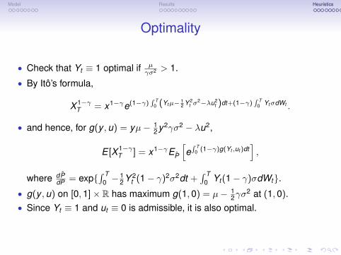
Model Results Heuristics
Conclusion
• Finite market depth. Execution price linear in volume as wealth turnover.• Representative agent with constant relative risk aversion.• Base price geometric Brownian Motion.• Trade towards frictionless portfolio.• Dynamics for trading volume.• Do not lever an illiquid asset!
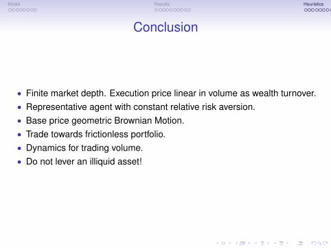

Model Results Heuristics
ERC Starting Grant
Market Frictions in Mathematical Finance
Dublin City University
Ph.D. and postdoc positions available.