Dynamic Routing Selection for Wireless SensorNetworks∗

W. Ke and T.D.C. LittleDepartment of Electrical and Computer Engineering

Boston University, Boston, Massachusetts{ke, tdcl}@bu.edu

June 2, 2008

MCL Technical Report No. 06-02-2008

Abstract–With the decrease in the cost and in the size of computing devices, wireless sensor net-works (WSNET) have the potential of being composed by an extremely large number of nodesoffering multiple services. Such networks have the capability of executing multiple tasks con-currently by allocating simply a fraction of their resources. Alternatively, many smaller wirelessnetworks may collaborate to execute a larger, unforeseen application. In both cases a routingscheme other than the prevailing one may improve the efficiency of the task or the applicationbeing executed, reducing the energy consumption in the network.

We posit that to fully tap into the potential of such networks a new routing infrastructure isneeded, one that allows switching between different routing schemes dynamically as required bythe applications being deployed, the conditions of the network as a whole and the existing localityinformation. We show in this paper how dynamic routing scheme selection can be achieved whensensor networks are overlaid with a virtual attribute based cluster hierarchy. We present analyticalresults for our scheme and show the expected improvement that can be achieved.

∗In Proc. Intl. Symp. on Network Computing and Applications (NCA 2008), July 11, 2008, Cambridge, MA. Thiswork is supported by the National Science Foundation under grant No. CNS-0435353. Any opinions, findings, andconclusions or recommendations expressed in this material are those of the author(s) and do not necessarily reflect theviews of the National Science Foundation.

1

1 Introduction

Subquadrant cluster leaderSubquadrant boundaryQuadrant boundary

Tree TraversalRepresentation

C−DAG

Subquadrant

Quadrant

Forest

Subquadrant

Quadrant

Forest

Mesh Traversal

������������

������������

������������

������������

������������

������������

������������������

������

������������������

� � � ���������

������������������

������������������

������������������

������������������

������������������

�������������������

�

��

!!""

Direction of Fire Propagation

FireDestroyed sensorForest cluster leaderQuadrant cluster leader

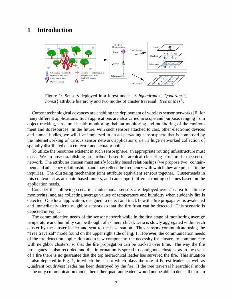
Figure 1: Sensors deployed in a forest under{Subquadrant⊂ Quadrant⊂Forest} attribute hierarchy and two modes of cluster traversal:Treeor Mesh.

Current technological advances are enabling the deployment of wireless sensor networks [6] formany different applications. Such applications are also varied in scope and purpose, ranging fromobject tracking, structural health monitoring, habitat monitoring and monitoring of the environ-ment and its resources. In the future, with such sensors attached to cars, other electronic devicesand human bodies, we will live immersed in an all pervading sensorsphere that is composed bythe internetworking of various sensor network applications, i.e., a huge networked collection ofspatially distributed data collector and actuator points.

To utilize the resources existent in such sensorsphere, an appropriate routing infrastructure mustexist. We propose establishing an attribute-based hierarchical clustering structure in the sensornetwork. The attributes chosen must satisfy locality based relationships (we propose two: contain-ment and adjacency relationships) and may reflect the frequency with which they are present in theinquiries. The clustering mechanism joins attribute equivalent sensors together. Clusterheads inthis context act as attribute-based routers, and can support different routing schemes based on theapplication needs.

Consider the following scenario: multi-modal sensors are deployed over an area for climatemonitoring, and are collecting average values of temperature and humidity when suddenly fire isdetected. One local application, designed to detect and track how the fire propagates, is awakenedand immediately alerts neighbor sensors so that the fire front can be detected. This scenario isdepicted in Fig. 1.

The communication needs of the sensor network while in the first stage of monitoring averagetemperature and humidity can be thought of as hierarchical. Data is slowly aggregated within eachcluster by the cluster leader and sent to the base station. Thus sensors communicate using the“Tree traversal” mode found on the upper right side of Fig. 1. However, the communication needsof the fire detection application add a new component: the necessity for clusters to communicatewith neighbor clusters, so that the fire propagation can be tracked over time. The way the firepropagates is also recorded and this information is spread to contiguous clusters, as in the eventof a fire there is no guarantee that the top hierarchical leader has survived the fire. This situationis also depicted in Fig. 1, in which the sensor which plays the role of Forest leader, as well asQuadrant SouthWest leader has been destroyed by the fire. If the tree traversal hierarchical modeis the only communication mode, then other quadrant leaders would not be able to detect the fire in

2

time. However, by using the “Mesh traversal” mode (lower right side of Fig. 1) at the lowest levelof the attribute hierarchy (Subquadrant clusters), sensors are able to spread the alarm and continuedetecting the fire front.

The example above illustrates how different applications may require different communicationpatterns. It is definitely possible, given the sensors are multi-modal [6] that other applications arealso present, e.g., wildlife tracking (needs to be able to communicate with neighboring sensors, toalert them of the tracked object, and needs to be able to send logged data back to base station),which would further drive the need for a common, yet flexible routing infrastructure [10].

We show in this paper how routing schemes can be built on top of attribute based hierarchicalclustering schemes, and demonstrate, through theoretical analysis, how switching between differ-ent traversal modes of the clusters result in higher gains for different metrics. We present in thenext section related work in the area. We delineate our design choices and show the basic func-tionality specification, as well as data structure and algorithms related to the implementation ofthe routing infrastructure in Sec. 3. We present theoretical performance analysis in Sec. 4 andconclude in Sec. 5.

2 Related Work

Past approaches such as diffusion [3, 7] flood inquiries to the network, and build gradients that col-lect data back. Such approach is limiting, for different applications may have different needs, andif sensor networks are shareable resources, then a single communication paradigm is not sufficientfor fully utilizing the resource. Moreover, if the sensor network is shared, requests may arrive forall different forms and types of data, causing frequent floods that may be irrelevant to most of thenodes in the network and wasting energy.

In order to reduce the redundant transmission of packets, location information is explored inorder to direct how data can be routed. GPSR (Greedy Perimeter Stateless Routing [8]) and GEAR(Geographical and Energy Aware Routing [16]) are two examples of geographical based routing.Both rely on the presence of location services to operate, and in both the addressing scheme isindependent of the applications they support. In other words, a data sink must knowa priori theregion to which send the data request and vice-versa. Data-centric models built on top of suchgeographic models, such as GHT [14], DIM [11], DIFS [5] and DIMENSIONS [4] do not offerlower level control over communication patterns that different applications may benefit from whentransmitting data.

Semantic Routing Trees (SRT) are proposed in [12], in which tree structures are formed in thesensor network based on sensed values and queries are forwarded to children that have valueswithin the range requested. Like SRT but with a more generalized filtering approach, CBCB(Combined Broadcast and Content Based routing [2]) adopts a two layer approach (one broadcastlayer and one content-based layer) to place predicates (a set of constraints on the attributes) atthe routers. Data that matches a predicate will be forwarded to the appropriate sinks. Our workdiffers from SRT and CBCB in that we do not attempt filtering at sensor level, but instead formattribute equivalent regions that help route traffic. We also support different communication needsand patterns in such regions.

The advantages of being able to select the routing protocol at run-time have been pointed outby the active network community [13]. Work in [15] proposes encapsulating packets in SAPF

3

(Simple Active Packet Format) headers, which carry indicators to an active node’s FIB (ForwardingInformation Base), guiding packet forwarding behavior at run-time. The routing example shownin [15] is tree based. In [1] the authors propose an overlay scheme that allows active nodes tocoexist with passive nodes. The active nodes track communication paths to each other reactively.Our work shows how dynamic routing protocol selection can be implemented in attribute clusteredWSNETs. We show the routing rules and the performance analysis for both the tree and the meshtraversal modes. Furthermore, we show how the changing density of “active routers” (in our caseattribute based routers or cluster leaders) in the network, achieved through changing the number oflevels in the attribute hierarchy, affects the expected performance of the two routing schemes. Wepresent in the next section our design choices and some basic functionality specification.

3 Routing

In traditional host centric routing schemes identifiers are given to network nodes that are indepen-dent of any attributes or data the host may possess. Such approach may be justified when in anetwork the emphasis is in finding the host, that is, data sets of interest map to a relatively fewhosts. However, in the situation in which multiple hosts share common data sets, reaching a spe-cific host is pointless, and the reversal situation should be attempted: to reach the data of interestrather than a specific host.

The challenge in such situations is to propose a scheme that can identify data sets of interest atvarying degrees of accuracy. We propose using an attribute hierarchy for this purpose. Attributehierarchies can be determined by each sensor network locally, have flexible degrees of accuracy(ranging from including all sensors in a large geographic region to being able to pinpoint specificsensors, given enough attributes), can be easily manipulated to provide basic units on top of whichrouting takes place (e.g., routing between rooms, or floors, or buildings), and can be overlaid (twoattribute hierarchies may be used by different applications to target the same set of sensors in dif-ferent ways, e.g., routing may happen between rooms, floors and buildings, or offices, departmentsand colleges).

We summarize next some design considerations and characteristics of one mechanism that canprovide a logical overlay of attribute based hierarchical clusters on the sensor network. Morespecific details can be found in [9].

3.1 Attribute Based Hierarchical Clustering

The set of attributes used to address sensors must satisfy containment relationships, that is, higherlevel attributes contain lower level attributes, and have all adjacency relationships defined, that is,which attribute values are spatially contiguous to each other. We represent containment relation-ships via directed acyclic graphs (C-DAG).

Nodes that have the same attributes are clustered together, and such clustering happens in ahierarchical manner. Each cluster represents an attribute-equivalent region, and by controllingwhich and how many attributes are part of the hierarchy we can control whether the propagationof inquiries is pure flooding (one level in the hierarchy), host centric (attributes have resolutionthat can pinpoint individual sensors uniquely), or a hybrid approach, in which we have attributeequivalent regions communicating with each other.

4

Once attribute equivalent regions have been established, clusterheads can coordinate intra- andinter-cluster data dissemination based on the application requirements. Currently we posit thatattributes should be selected based on ana priori assumption on the frequency such attributeswill be called by users in their inquiries. We support dynamic modifications to the C-DAG afterdeployment to insert or remove nodes to more efficiently guide data propagation. For more detailson the clustering process, see [9].

Table 1: Different Routing Schemes – (a)Left: Tree traversal, (b)Right: Mesh traversal)1: CDAG← {Subquadrant ⊂Quadrant ⊂ Forest};2: RoutingTable← Routing table used by current application;3: SensorAttributes← Attributes current sensor possesses;4: SensorClusters← Set of clusters the current sensor belongs to;5: SensorClusterLeader← Set of clusters the current sensor is leader

of;6: N (X, Y ) = function that returns the number of consecutively

matched attributes betweenX and Y , starting from the first at-tribute in bothX andY ;

7: Received packetP;8: DestAttrList← list of attribute name-value pairs of the destination

in P;9: FindE ∈ RoutingTable| (N (DestAttrList,E) is maximized) ;

10: if (E = DestAttrList) then11: if (E ∈ SensorClusters) then12: FloodP in E; Return;13: else if (P.PrevHop 6∈ {path between current sensor∧ E})

then14: SendP to E; Return;15:16: if (∃ L ∈ SensorClusterLeader| (L = P.NextHop )) then17: if (P.PrevHop is parent node inCDAG) ∨ (sensor is root

leader)then18: if (∃ children node| known attributes of children node match

DestAttrList) then19: SendP to children node inCDAG;20: else21: Drop packetP;22: else23: if (∃ unmatched attribute at levelL or higher between the

sensor andDestAttrList) then24: SendP to parent ofL;25: else if (all attributes from root to levelL match between

the sensor andDestAttrList∧ ∃ child cluster with increasedattribute match)then

26: SendP to sibling clusters;27: SendP to child cluster;28: else29: DropP;30: else31: SendP to leader ofP.NextHop ;

1: CDAG← {Subquadrant ⊂Quadrant ⊂ Forest};2: RoutingTable← Routing table used by current application;3: SensorClusters← Set of clusters the current sensor belongs to;4: SensorClusterLeader← Set of clusters the current sensor is leader

of;5: N (X, Y ) = function that returns the number of consecutively

matched attributes betweenX and Y , starting from the first at-tribute in bothX andY ;

6: Received packetP;7: if (P was received before)then8: Return;9: DestAttrList← list of attribute name-value pairs of the destination

in P;10: FindE ∈ RoutingTable| (N (DestAttrList,E) is maximized) ;11: if (E = DestAttrList) then12: if (E ∈ SensorClusters) then13: FloodP in E; Return;14: else if (P.PrevHop 6∈ {path between current sensor∧ E})

then15: SendP to E; Return;16:17: if (∃ L ∈ SensorClusterLeader| (L = P.NextHop )) then18: if (∃ children node| known attributes of children node match

DestAttrList) then19: SendP to children node inCDAG;20: else if (∃ adjacent clusterC at same level ofL with matching

attribute∧ no copy ofP came fromC) then21: ForwardP to all suchC;22: else23: DropP;24: else25: SendP to leader ofP.NextHop ;

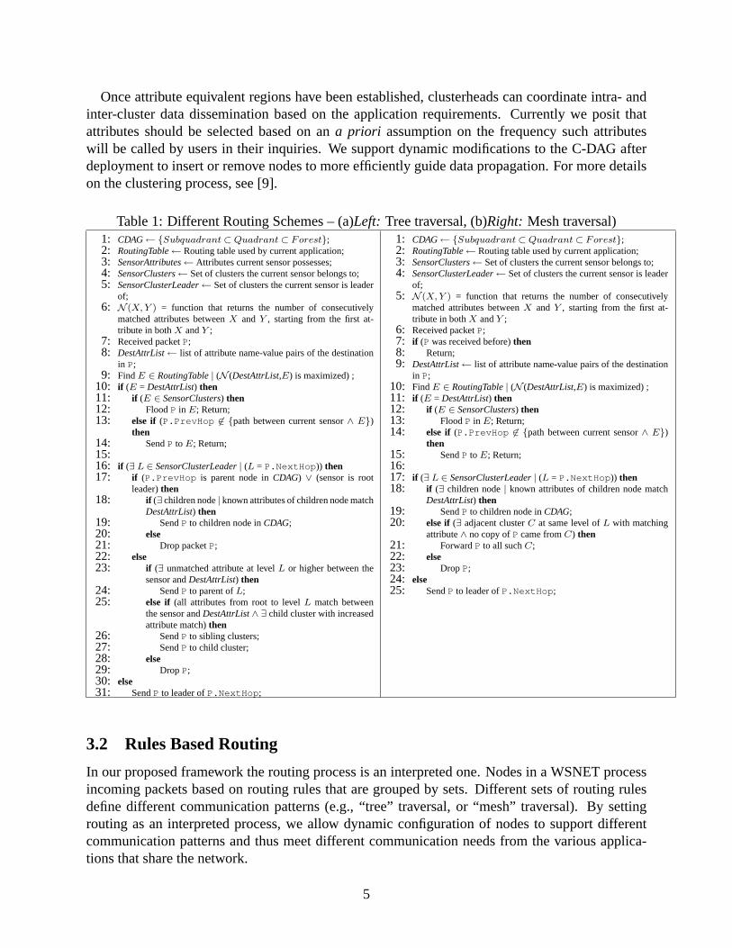
3.2 Rules Based Routing

In our proposed framework the routing process is an interpreted one. Nodes in a WSNET processincoming packets based on routing rules that are grouped by sets. Different sets of routing rulesdefine different communication patterns (e.g., “tree” traversal, or “mesh” traversal). By settingrouting as an interpreted process, we allow dynamic configuration of nodes to support differentcommunication patterns and thus meet different communication needs from the various applica-tions that share the network.

5

Each “rule” in our rules based routing is composed of two parts: (1) a conditional statementand (2) an action statement. If the conditions specified are true, then the action is carried out.Otherwise, the following rule in the rule set is checked. If no conditional statement turns out trueafter going through all the rules, the packet is simply dropped. Our rules based approach essentiallyimposes a priority scheme over possible next-hop destinations.

In the right side of Fig. 1 two communication patterns can be established, the “HierarchicalTree Traversal” mode, in which lower level cluster leaders communicate with higher level clusterleaders, routing in a hierarchical virtual tree, or the “Mesh Traversal” mode, in which clusterleaders at the lowest level in the C-DAG communicate with adjacent cluster leaders, routing on alogical mesh. Routing rules for both traversal modes are shown in Table 1. In the tree traversal,unknown destination packets may be sent to higher level cluster leaders (Line 24 of Table 1a),and these may eventually forward the packets back (Line 27 of Table 1a). The Mesh traversalalgorithm forwards packets of unresolved attributes to neighbor clusters (Line 21 in Table 1b).Notice the different approach each routing rule establishes on resolving unknown addresses: whilein the tree case the packets are forwarded up the hierarchy level, in the mesh the packets are simplyspread towards other adjacent clusters. These two resolution modes also characterize the intrinsiccommunication pattern each rules set supports. Sensor networks that are deployed for differentapplications will benefit from being able to support switching between the two modes, as we willshow in the next section.

4 Performance Analysis

In this section we study the performance of the Mesh routing scheme represented by Table 1 asapplied to a “line” C-DAG (center of Fig. 1), and of schemes that rely on “flooding” for datapropagation, as well as schemes that have full knowledge of all sensors in the network. Due tospace limitations we will offer only analysis on the Mesh traversal scheme. Readers are referredto [10] for analysis on the Tree traversal scheme details.

The network is consisted ofN sensors spread uniformly over a square region of areaL2 andthere arelh levels in the line attribute hierarchy. Since the C-DAG representation of the attributehierarchy is a line, there arelh nodes in the C-DAG. The root node (at level1) in the C-DAG coversthe whole region, while subsequent nodes (at levelsli, i ∈ {2, . . . , lh}) have four possible valueseach (a quadtree format), with each value covering a square region of sideL/2(i−1). In the right ofFig. 1 a three level C-DAG is shown.

The metrics we will be studying for each scheme include: (1) total memory requirement fromall nodes for implementation; (2) the estimated number of transmissions taken when routing onepacket from a source to an unknown destination in the worst case (considering that the sensors aredeployed over a square region, the worst case is when source and destination lie at opposite cornersacross a diagonal) and (3) the estimated number of hops that separate source from destination afterthe destination’s address has been “resolved” in (2). Essentially (1) allows us to gauge how scal-able each scheme is in terms of the amount of memory needed. Metric (2) allows us to compare thecost of resolving an unknown destination address, while (3) is an estimate of how quickly the des-tination address can be found or how quickly data can be transmitted to the destination, assumingboth being directly proportional to the hop distance that separates source from destination.

When estimating item (2) and (3) above, for non-flooding type of schemes, we consider that

6

the path the packet takes is composed of consecutive straight line segments. One estimate of thenumber of transmissions (or the number of hops) is the product of the length of the segment bythe linear node density. The node density is given byρ = N/L2, thus one estimate of the numberof neighbors that lie on a line segment within transmission radiusR is R

√ρ. On the average,

assuming the sensors are uniformly distributed and the whole network connected, the number oftransmissions should not be greater than this value, for this value reflects the number nodes thatlie in the segment. If this value is� 1, then we are overestimating the number of transmissionsneeded. Estimates made in this way can still be used for comparison between different routingschemes, though, since the overestimation comes from the high node density value and will bereflected by all routing schemes.

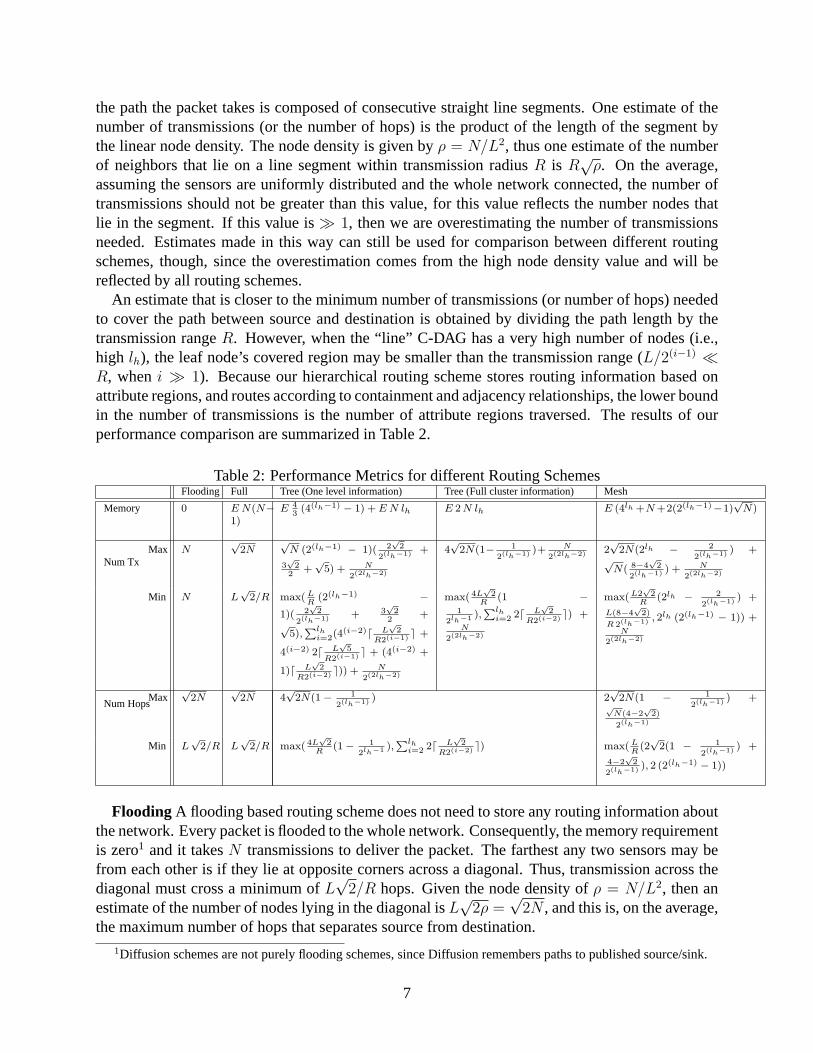
An estimate that is closer to the minimum number of transmissions (or number of hops) neededto cover the path between source and destination is obtained by dividing the path length by thetransmission rangeR. However, when the “line” C-DAG has a very high number of nodes (i.e.,high lh), the leaf node’s covered region may be smaller than the transmission range (L/2(i−1) �R, wheni � 1). Because our hierarchical routing scheme stores routing information based onattribute regions, and routes according to containment and adjacency relationships, the lower boundin the number of transmissions is the number of attribute regions traversed. The results of ourperformance comparison are summarized in Table 2.

Table 2: Performance Metrics for different Routing SchemesFlooding Full Tree (One level information) Tree (Full cluster information) Mesh

Memory 0 E N(N−1)

E 43

(4(lh−1) − 1) + E N lh E 2 N lh E (4lh +N +2(2(lh−1)−1)√

N)

Num TxMax N

√2N

√N (2(lh−1) − 1)( 2

√2

2(lh−1) +

3√

22

+√

5) + N

2(2lh−2)

4√

2N(1− 1

2(lh−1) )+ N

2(2lh−2) 2√

2N(2lh − 2

2(lh−1) ) +√

N( 8−4√

2

2(lh−1) ) + N

2(2lh−2)

Min N L√

2/R max( LR

(2(lh−1) −1)( 2

√2

2(lh−1) + 3√

22

+√

5),Plh

i=2(4(i−2)d L√

2R2(i−1) e +

4(i−2) 2d L√

5R2(i−1) e + (4(i−2) +

1)d L√

2R2(i−2) e)) + N

2(2lh−2)

max( 4L√

2R

(1 −1

2lh−1 ),Plh

i=2 2d L√

2R2(i−2) e) +

N

2(2lh−2)

max(L2√

2R

(2lh − 2

2(lh−1) ) +

L(8−4√

2)

R 2(lh−1) , 2lh (2(lh−1) − 1)) +N

2(2lh−2)

Num HopsMax

√2N

√2N 4

√2N(1− 1

2(lh−1) ) 2√

2N(1 − 1

2(lh−1) ) +√

N(4−2√

2)

2(lh−1)

Min L√

2/R L√

2/R max( 4L√

2R

(1− 1

2lh−1 ),Plh

i=2 2d L√

2R2(i−2) e) max( L

R(2√

2(1 − 1

2(lh−1) ) +

4−2√

2

2(lh−1) ), 2 (2(lh−1) − 1))

Flooding A flooding based routing scheme does not need to store any routing information aboutthe network. Every packet is flooded to the whole network. Consequently, the memory requirementis zero1 and it takesN transmissions to deliver the packet. The farthest any two sensors may befrom each other is if they lie at opposite corners across a diagonal. Thus, transmission across thediagonal must cross a minimum ofL

√2/R hops. Given the node density ofρ = N/L2, then an

estimate of the number of nodes lying in the diagonal isL√

2ρ =√

2N , and this is, on the average,the maximum number of hops that separates source from destination.

1Diffusion schemes are not purely flooding schemes, since Diffusion remembers paths to published source/sink.

7

Full Knowledge A routing scheme that stores next hop routing information for all nodes inthe network has a huge memory requirement. In fact, each node needs to store information aboutN − 1 other nodes in the network. Considering that each routing entry requiresE bytes, the totalmemory requirement in the network isE N(N−1). However, because of the complete knowledge,the number of transmissions triggered and the number of transmissions needed to send the packetare equal. These are equal to the estimated maximum and minimum number of hops in the floodingcase.

Cluster Flooding In both Flooding andFull Knowledgeschemes destination sensors are sureto be reached. In “Tree” or “Mesh” schemes below, however, packets reaching the intendedleaf cluster(s) still need to reach the sensors. Assuming the intended destination address “re-solves” into one leaf cluster, to flood that cluster the number of additional transmissions is equalto ρ (L/2(lh−1))2 = N/2(2lh−2) is needed. This term appears in all “NumTx” entries in Table 2.

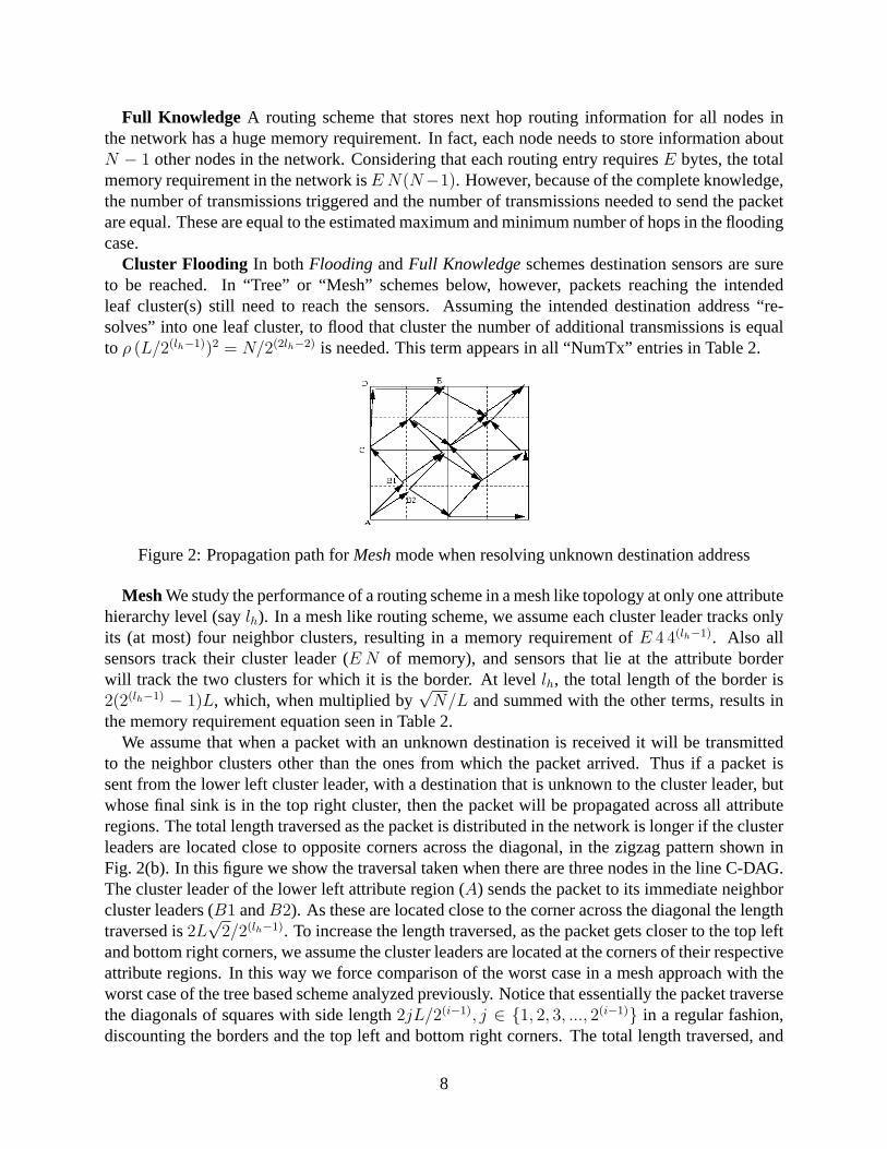
Figure 2: Propagation path forMeshmode when resolving unknown destination address

MeshWe study the performance of a routing scheme in a mesh like topology at only one attributehierarchy level (saylh). In a mesh like routing scheme, we assume each cluster leader tracks onlyits (at most) four neighbor clusters, resulting in a memory requirement ofE 4 4(lh−1). Also allsensors track their cluster leader (E N of memory), and sensors that lie at the attribute borderwill track the two clusters for which it is the border. At levellh, the total length of the border is2(2(lh−1) − 1)L, which, when multiplied by

√N/L and summed with the other terms, results in

the memory requirement equation seen in Table 2.We assume that when a packet with an unknown destination is received it will be transmitted

to the neighbor clusters other than the ones from which the packet arrived. Thus if a packet issent from the lower left cluster leader, with a destination that is unknown to the cluster leader, butwhose final sink is in the top right cluster, then the packet will be propagated across all attributeregions. The total length traversed as the packet is distributed in the network is longer if the clusterleaders are located close to opposite corners across the diagonal, in the zigzag pattern shown inFig. 2(b). In this figure we show the traversal taken when there are three nodes in the line C-DAG.The cluster leader of the lower left attribute region (A) sends the packet to its immediate neighborcluster leaders (B1 andB2). As these are located close to the corner across the diagonal the lengthtraversed is2L

√2/2(lh−1). To increase the length traversed, as the packet gets closer to the top left

and bottom right corners, we assume the cluster leaders are located at the corners of their respectiveattribute regions. In this way we force comparison of the worst case in a mesh approach with theworst case of the tree based scheme analyzed previously. Notice that essentially the packet traversethe diagonals of squares with side length2jL/2(i−1), j ∈ {1, 2, 3, ..., 2(i−1)} in a regular fashion,discounting the borders and the top left and bottom right corners. The total length traversed, and

8

the corresponding expected number of transmissions (both maximum and minimum) are given bythe corresponding expressions in Table 3.

When the transmission radiusR � L/2(i−1), then it takes at least one transmission to crossone attribute region, and assuming each attribute region will transmit to two of its immediateneighbors (with top and right border attribute regions transmitting only once), the total number oftransmissions will be2(2(lh−1) − 1) + 2(2(lh−1) − 1)2 = 2lh(2(lh−1) − 1), as seen in the table.

The shortest path that separates the source from the destination must traverse2(2(lh−1) − 1) + 1attribute regions (the+1 is because the source attribute region also must be traversed). However, ifthe packet goes through only the diagonals, only2(2(lh−1) − 1) diagonals need be crossed. One ofthe attribute region leaders will receive the packet from the left and can immediately forward to theupper region, without needing to traverse itself. Thus the worst case scenario is actually when thesource is at the top left corner while the destination is at the bottom right corner (or vice-versa). Inthis case there are additional four traversals across the border of the attribute region (4(L/2(lh−1)))and two less diagonal traversals. This explains the second term in the “NumHopMax” and thesecond term in the first argument to themax function in “NumHopMin.” When we are consideringthe minimum number of hops, this must be lower bounded by the number of attribute regions thatneed be crossed (2(2(lh−1) − 1)), since in principle the cluster leader only tracks the four adjacentclusters. We show some plots of the equations of Table 2 in Fig. 3.

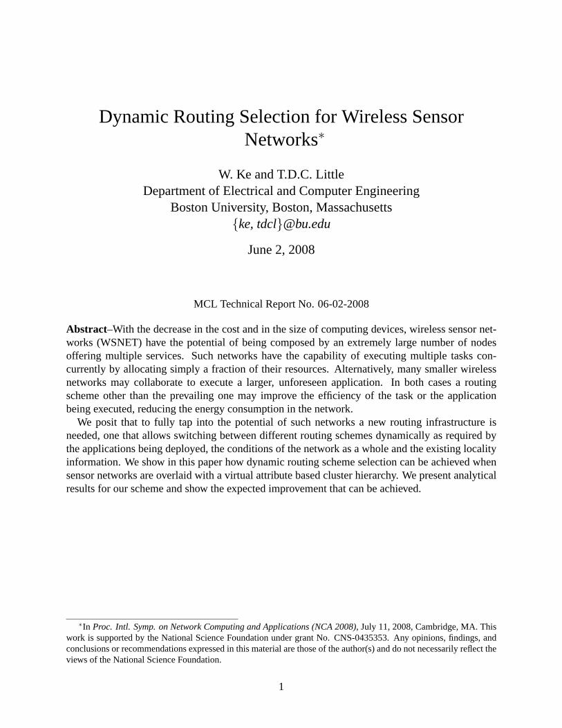
We can see from Fig. 3(a) and Fig. 3(b) that the expected number of transmissions to resolve anunknown address in the worst case is higher for the Mesh traversal mode than for the Tree cases.In fact, when cluster leaders track full cluster information, the performance dramatically improves.This is because the root node need not propagate the packet with unknown address down to all of itschildren clusters. We can see that the high number of levels in the attribute hierarchy contributes tothe inefficiency of the process (Fig. 3(b) and 3(e)). With the increase in the number of hierarchies,the packet with unknown destination address need essentially be distributed to the whole networkin the Mesh and Tree (with one level information) schemes at increasing levels of granularity (i.e.,covering more of the network), contributing to their performance degradation.

A high number of levels will involve transmission costs to cross adjacent clusters in the Meshcase and costs to resolve all the way to the leaf cluster in the Tree (one level info) case. Thesecosts surpass those of the mere flooding schemes and should be avoided. The cost for resolvingan unknown address in the Tree (full cluster info) case remains constant. However, the memoryrequirements are high (Figs. 3(c) and 3(f)).

When we consider the number of hops metric, we find that Mesh schemes are able to findshorter paths between source and destination. The only drawback is that Mesh schemes currentlyonly cross spatially adjacent attribute regions. Thus when the number of levels in the hierarchyincreases, there is a corresponding increase in the hop distance (Figs. 3(h) and 3(i)).

From the graphs in Fig. 3 we can see that if the network is composed of heterogeneous nodes,in which some nodes have higher capacity, then a Tree (full cluster info) scheme will be the mosteconomical in transmission costs related to address resolution issues. Sensor networks that havea high inquiry arrival, especially from a large user base, will benefit from the increased savingsin Tree based address resolution schemes, while applications that require fast response can invokeMesh traversal mode for their data packets.

9

5 Conclusion

In this paper we presented examples of different applications being tasked to the same sensor net-work simultaneously. Due to the different objectives of the applications, their underlying data com-munication and dissemination patterns favor different routing schemes. We envision that sensornetworks will be widespread in the future. and to tap into the full potential of such sensorsphere,the underlying routing infrastructure must support dynamic routing scheme selection. With thisfeature, tasked applications can request routing support from a scheme whose packet forwardingrules match their data communication requirements, thus maximizing their performance.

In order to enable dynamic routing scheme selection, we propose using sets of routing rulesthat forward data in pre-defined ways as the elements to be selected at runtime. We assume thatthe underlying sensor network has been clustered according to a hierarchy of attributes, and thatcontainment and adjacency relationships between the clusters (or the attributes) are clearly defined.We present in this paper two routing rules set for applications deployed in a sensor network with theabove mentioned logical structure. One rules set implements Tree traversal mode while the otherMesh traversal mode. We show analytical performance results of the two traversal modes and showthat Mesh traversal mode favors applications that need fast response, while Tree traversal mode hasless transmission cost when resolving a previously unknown destination address.

References

[1] S. Calomme and G. Leduc. Performance Study of an Overlay Approach to Active Routing in Ad HocNetworks. InProc. 3rd Annual Mediterranean Ad Hoc Networking Workshop (Med-Hoc-Net 2004),Bodrum, Turkey, Jun 2004.

[2] A. Carzaniga, M. J. Rutherford, and A. L. Wolf. A Routing Scheme for Content-Based Networking.In Proc. IEEE INFOCOM’04, Hong Kong, China, 2004.

[3] D. Estrin, R. Govindan, J. Heidemann, and S. Kumar. Next Century Challenges: Scalable Coordina-tion in Sensor Networks. InProc. 5th ACM MobiCom Conference, Seattle, WA, August 1999.

[4] D. Ganesan, D. Estrin, and J. Heidemann. DIMENSIONS: Why do we need a new Data Handlingarchitecture for Sensor Networks? InProc. 1st Workshop on Hot Topics In Networks (HotNets-I),Princeton, NJ, October 2002.

[5] B. Greenstein, D. Estrin, R. Govindan, S. Ratnasamy, and S. Shenker. DIFS: A Distributed Index forFeatures in Sensor Networks. InProc. 1st IEEE Intl. Workshop on Sensor Network Protocols andApplications (SNPA’03), 2003.

[6] J. Hill and D. Culler. MICA: A Wireless Platform For Deeply Embedded Networks.IEEE Micro,22(6):12–24, Nov/Dec 2002.

[7] C. Intanagonwiwat, R. Govindan, and D. Estrin. Directed Diffusion: A Scalable and Robust Commu-nication Paradigm for Sensor Networks. InProc. International Conference on Mobile Computing andNetworking (MobiCom), Boston, MA, August 2000.

[8] B. Karp and H. T. Kung. Greedy Perimeter Stateless Routing for Wireless Networks. InProceedingsof the 6th ACM MobiCom Conference, pages 243–254, Boston, MA, August 2000.

[9] W. Ke, S. A. Ayyash, P. Basu, and T. D. C. Little. Attribute-Based Clustering for Information Dissem-ination in Wireless Sensor Networks. InProc. 2nd Annual IEEE Communications Society Conferenceon Sensor and Ad Hoc Communications and Networks (SECON’05), Sant Clara, CA, USA, September2005.

10

[10] W. Ke and T. D. C. Little. Dynamic Route Selection for Wireless Sensor Networks. Technical report,Boston University, 2006. MCL Technical Report 05-02-2006http://hulk.bu.edu/pubs/papers/2006/TR-05-02-2006.pdf .

[11] X. Li, Y. J. Kim, R. Govindan, and W. Hong. Multi-dimensional Range Queries in Sensor Networks.In Proc. 1st ACM Intl. Conference on Embedded Networked Sensor Systems (Sensys’03), Los Angeles,CA, USA, November 2003.

[12] S. Madden, M. Franklin, J. Hellerstein, and W. Hong. The Design of an Acquisitional Query Processorfor Sensor Networks. InProc. ACM SIGMOD, San Diego, CA, June. 2003.

[13] C. Prehofer and Q. Wei. Active Networks for 4G Mobile Communication: Motivation, Architecture,and Application Scenarios. InProc. IFIP-TC6 International Working Conference (IWAN’02), London,UK, 2002.

[14] S. Ratnasamy, B. Karp, L. Yin, F. Yu, D. Estrin, R. Govindan, and S. Shenker. GHT: A GeographicHash Table for Data-Centric Storage. InProc. 1st ACM Intl. Workshop on Wireless Sensor Networksand Applications (WSNA’02), Atlanta, GA, September 2002.

[15] C. Tschudin, H. Gulbrandsen, and H. Lundgren. Active routing for ad-hoc networks.IEEE Commu-nications Magazine, Special issue on Active and Programmable Networks, April 2000.

[16] Y. Yu, R. Govindan, and D. Estrin. Geographical and Energy Aware Routing: A Recursive DataDissemination Protocol for Wireless Sensor Networks. Technical report, UCLA Computer ScienceDepartment Technical Report UCLA/CSD-TR-01-0023, May 2001.

11

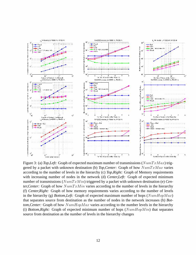
Figure 3: (a)Top,Left:Graph of expected maximum number of transmissions (NumTxMax) trig-gered by a packet with unknown destination (b)Top,Center:Graph of howNumTxMax variesaccording to the number of levels in the hierarchy (c)Top,Right:Graph of Memory requirementswith increasing number of nodes in the network (d)Center,Left: Graph of expected minimumnumber of transmissions (NumTxMin) triggered by a packet with unknown destination (e)Cen-ter,Center:Graph of howNumTxMin varies according to the number of levels in the hierarchy(f) Center,Right:Graph of how memory requirements varies according to the number of levelsin the hierarchy (g)Bottom,Left:Graph of expected maximum number of hops (NumHopMax)that separates source from destination as the number of nodes in the network increases (h)Bot-tom,Center:Graph of howNumHopMax varies according to the number levels in the hierarchy(i) Bottom,Right:Graph of expected minimum number of hops (NumHopMin) that separatessource from destination as the number of levels in the hierarchy changes

12