Dynamic Response Properties and Longitudinal Static Stability of CIrrus SR22

AAE 490A: Experiment # 5 – Dynamic Response Properties and Longitudinal Static Stability

Team 1 1

AAE 490A / AT490 Flight Testing

Experiment # 5

Dynamic Response Properties and Longitudinal Static Stability Cirrus SR22

Team 1 Xavier Thierry – [email protected]

Christopher Warner – [email protected] Ryan Harmeyer – [email protected]

Professor: Dr. Dominick Andrisani

TA: Saverio Rotella

Purdue University, School of Aeronautics and Astronautics Engineering

Experiment Performed: 04/08/2014

Report Submitted: 04/30/2014


Team 1 2

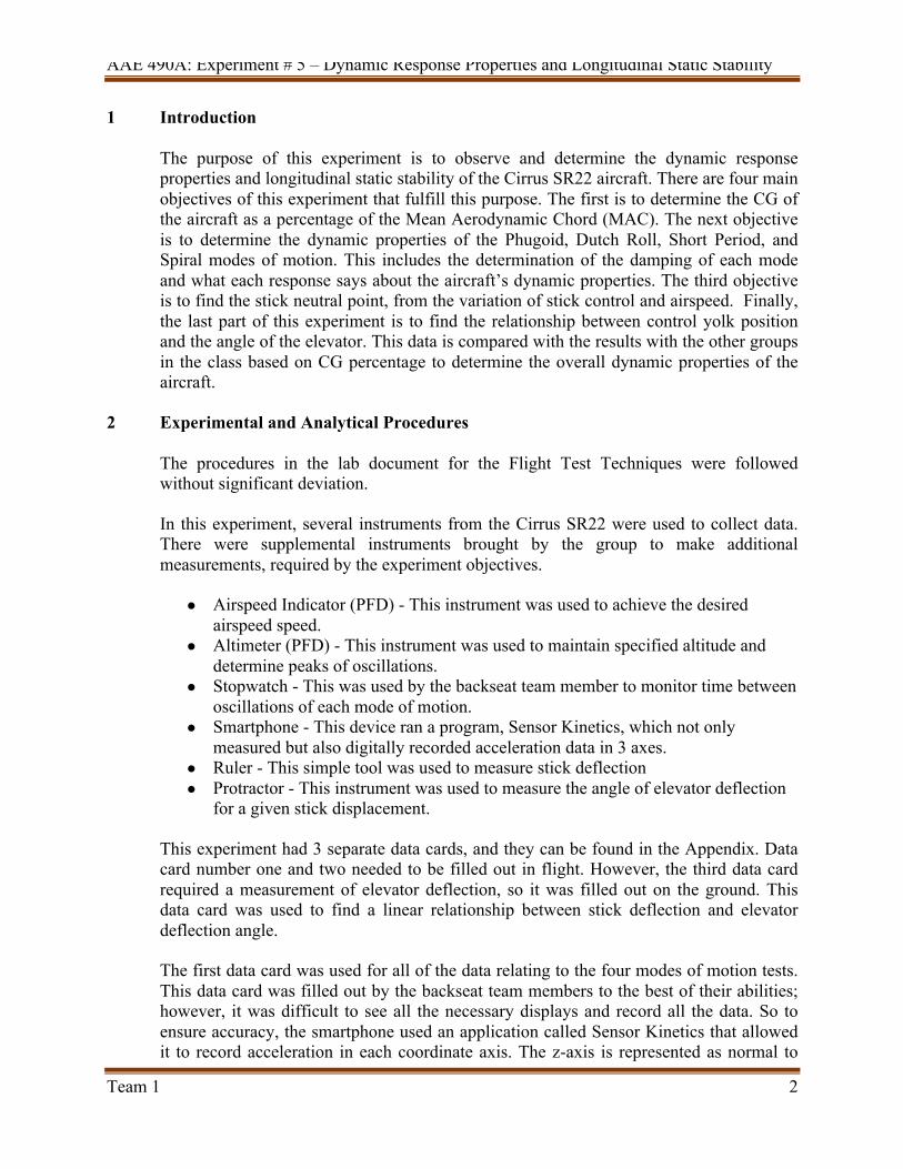
1 Introduction The purpose of this experiment is to observe and determine the dynamic response properties and longitudinal static stability of the Cirrus SR22 aircraft. There are four main objectives of this experiment that fulfill this purpose. The first is to determine the CG of the aircraft as a percentage of the Mean Aerodynamic Chord (MAC). The next objective is to determine the dynamic properties of the Phugoid, Dutch Roll, Short Period, and Spiral modes of motion. This includes the determination of the damping of each mode and what each response says about the aircraft’s dynamic properties. The third objective is to find the stick neutral point, from the variation of stick control and airspeed. Finally, the last part of this experiment is to find the relationship between control yolk position and the angle of the elevator. This data is compared with the results with the other groups in the class based on CG percentage to determine the overall dynamic properties of the aircraft.

2 Experimental and Analytical Procedures The procedures in the lab document for the Flight Test Techniques were followed without significant deviation. In this experiment, several instruments from the Cirrus SR22 were used to collect data. There were supplemental instruments brought by the group to make additional measurements, required by the experiment objectives.

● Airspeed Indicator (PFD) - This instrument was used to achieve the desired airspeed speed.

● Altimeter (PFD) - This instrument was used to maintain specified altitude and determine peaks of oscillations.

● Stopwatch - This was used by the backseat team member to monitor time between oscillations of each mode of motion.

● Smartphone - This device ran a program, Sensor Kinetics, which not only measured but also digitally recorded acceleration data in 3 axes.

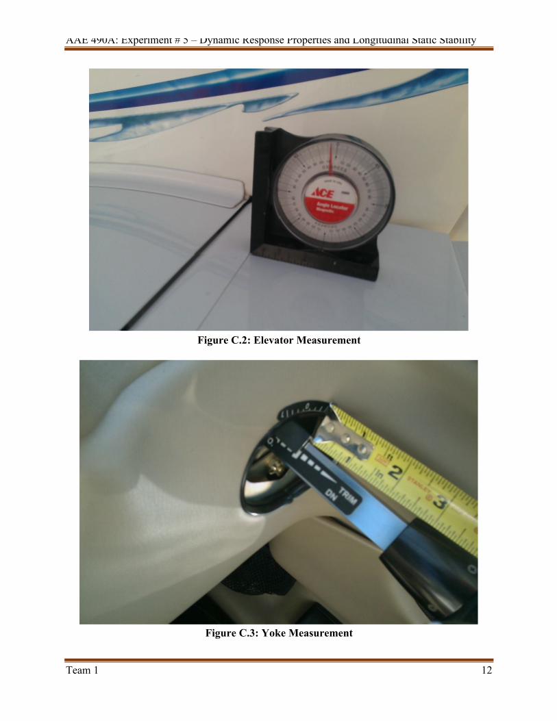
● Ruler - This simple tool was used to measure stick deflection ● Protractor - This instrument was used to measure the angle of elevator deflection

for a given stick displacement.

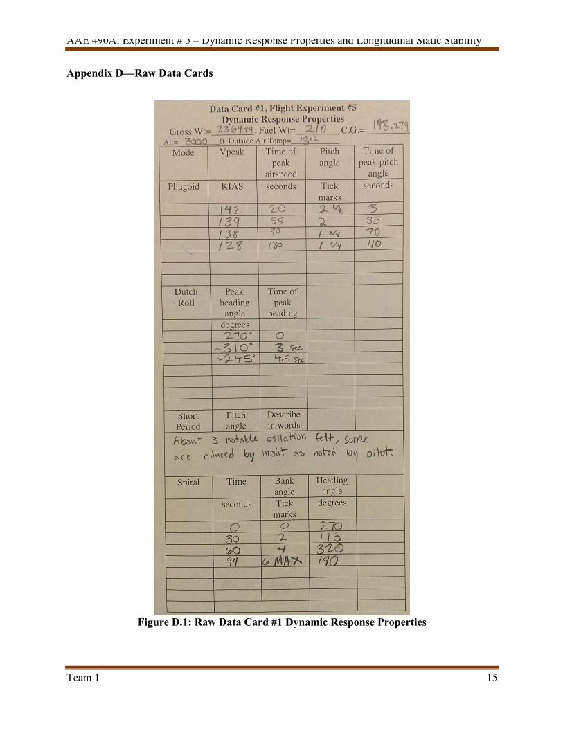
This experiment had 3 separate data cards, and they can be found in the Appendix. Data card number one and two needed to be filled out in flight. However, the third data card required a measurement of elevator deflection, so it was filled out on the ground. This data card was used to find a linear relationship between stick deflection and elevator deflection angle. The first data card was used for all of the data relating to the four modes of motion tests. This data card was filled out by the backseat team members to the best of their abilities; however, it was difficult to see all the necessary displays and record all the data. So to ensure accuracy, the smartphone used an application called Sensor Kinetics that allowed it to record acceleration in each coordinate axis. The z-axis is represented as normal to


Team 1 3

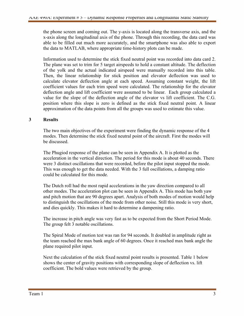
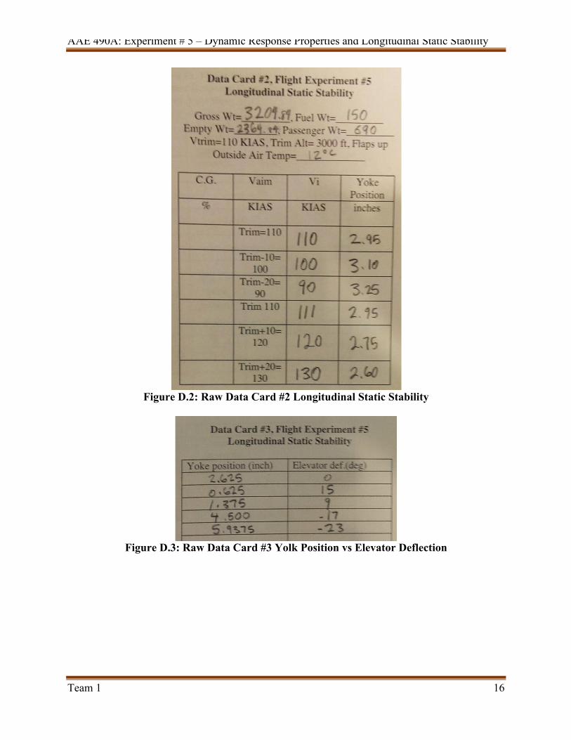
the phone screen and coming out. The y-axis is located along the transverse axis, and the x-axis along the longitudinal axis of the phone. Through this recording, the data card was able to be filled out much more accurately, and the smartphone was also able to export the data to MATLAB, where appropriate time-history plots can be made. Information used to determine the stick fixed neutral point was recorded into data card 2. The plane was set to trim for 5 target airspeeds to hold a constant altitude. The deflection of the yolk and the actual indicated airspeed were manually recorded into this table. Then, the linear relationship for stick position and elevator deflection was used to calculate elevator deflection angle at each speed. Assuming constant weight, the lift coefficient values for each trim speed were calculated. The relationship for the elevator deflection angle and lift coefficient were assumed to be linear. Each group calculated a value for the slope of the deflection angle of the elevator vs lift coefficient. The C.G. position where this slope is zero is defined as the stick fixed neutral point. A linear approximation of the data points from all the groups was used to estimate this value.

3 Results

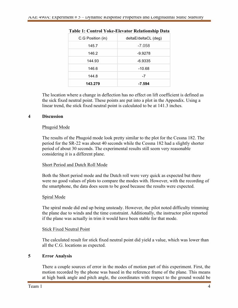
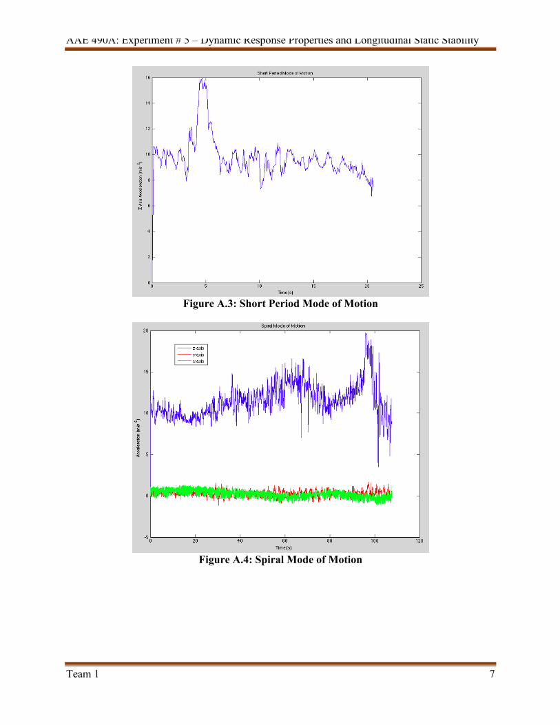
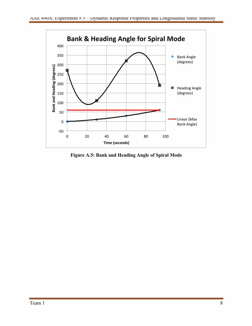
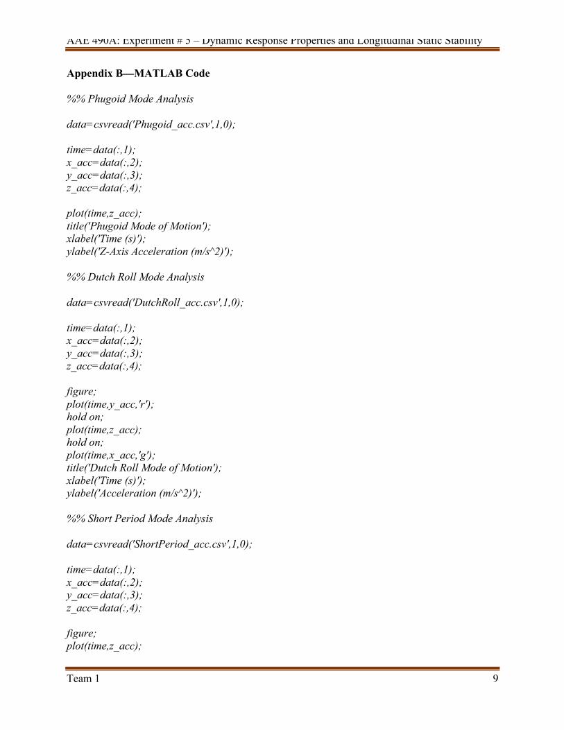
The two main objectives of the experiment were finding the dynamic response of the 4 modes. Then determine the stick fixed neutral point of the aircraft. First the modes will be discussed. The Phugiod response of the plane can be seen in Appendix A. It is plotted as the acceleration in the vertical direction. The period for this mode is about 40 seconds. There were 3 distinct oscillations that were recorded, before the pilot input stopped the mode. This was enough to get the data needed. With the 3 full oscillations, a damping ratio could be calculated for this mode. The Dutch roll had the most rapid accelerations in the yaw direction compared to all other modes. The acceleration plot can be seen in Appendix A. This mode has both yaw and pitch motion that are 90 degrees apart. Analysis of both modes of motion would help to distinguish the oscillations of the mode from other noise. Still this mode is very short, and dies quickly. This makes it hard to determine a dampening ratio. The increase in pitch angle was very fast as to be expected from the Short Period Mode. The group felt 3 notable oscillations. The Spiral Mode of motion test was ran for 94 seconds. It doubled in amplitude right as the team reached the max bank angle of 60 degrees. Once it reached max bank angle the plane required pilot input. Next the calculation of the stick fixed neutral point results is presented. Table 1 below shows the center of gravity positions with corresponding slope of deflection vs. lift coefficient. The bold values were retrieved by the group.


Team 1 4

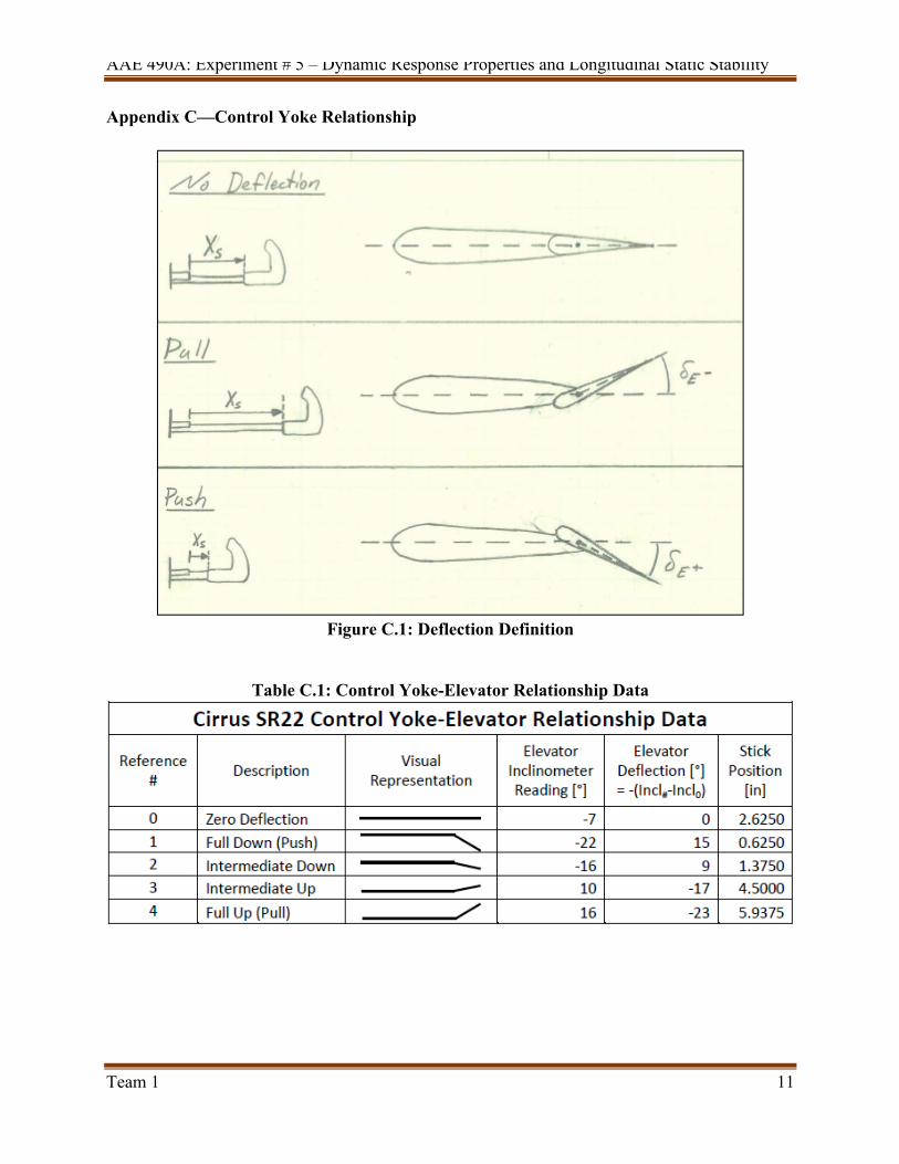
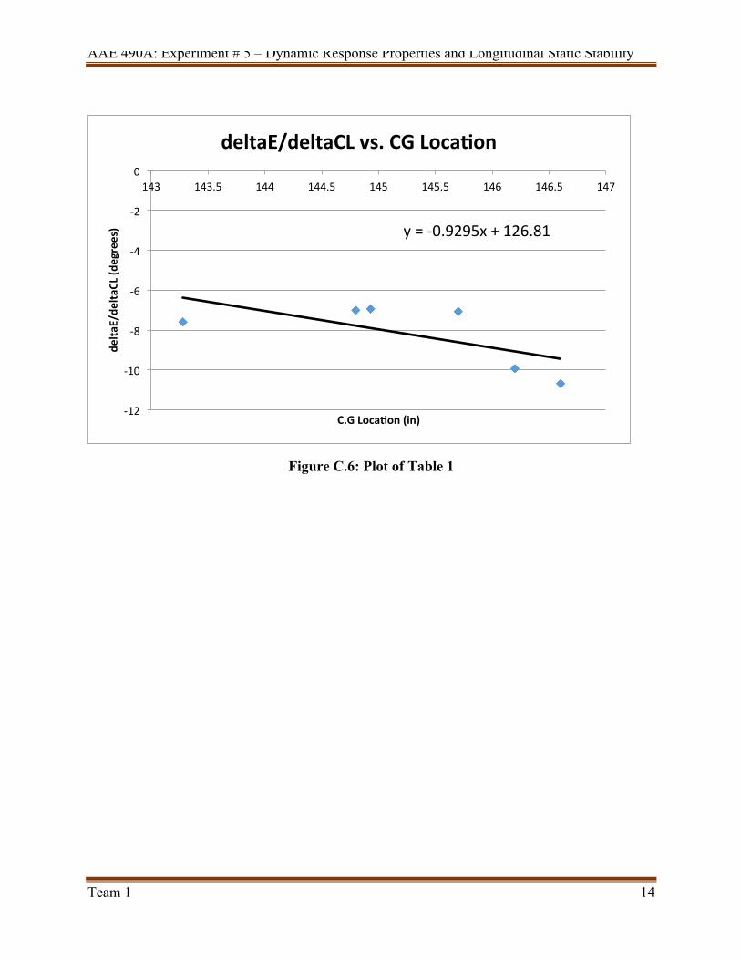
Table 1: Control Yoke-Elevator Relationship Data C.G Position (in) deltaE/deltaCL (deg)

145.7 -7.058

146.2 -9.9278

144.93 -6.9335

146.6 -10.68

144.8 -7

143.279 -7.594 The location where a change in deflection has no effect on lift coefficient is defined as the sick fixed neutral point. These points are put into a plot in the Appendix. Using a linear trend, the stick fixed neutral point is calculated to be at 141.3 inches.

4 Discussion

Phugoid Mode The results of the Phugoid mode look pretty similar to the plot for the Cessna 182. The period for the SR-22 was about 40 seconds while the Cessna 182 had a slightly shorter period of about 30 seconds. The experimental results still seem very reasonable considering it is a different plane. Short Period and Dutch Roll Mode Both the Short period mode and the Dutch roll were very quick as expected but there were no good values of plots to compare the modes with. However, with the recording of the smartphone, the data does seem to be good because the results were expected. Spiral Mode The spiral mode did end up being unsteady. However, the pilot noted difficulty trimming the plane due to winds and the time constraint. Additionally, the instructor pilot reported if the plane was actually in trim it would have been stable for that mode. Stick Fixed Neutral Point The calculated result for stick fixed neutral point did yield a value, which was lower than all the C.G. locations as expected.

5 Error Analysis

There a couple sources of error in the modes of motion part of this experiment. First, the motion recorded by the phone was based in the reference frame of the plane. This means at high bank angle and pitch angle, the coordinates with respect to the ground would be


Team 1 5

tilted. There was no way to record the angle of attack of the plan. This measurement is especially important to determine the response of the short period mode. Locating the stick fixed neutral point has a couple sources as well. The largest source of the error in this calculation is the measurement of the yolk position at the 5 different trim speeds by each group. Even though all groups used the same data for yolk position vs deflection angle of the elevator, each group did not measure stick position from the same references. This is shown in the complied data reduction in the Appendix by a wide range of trimmed deflection angle for the same speed. Also a smaller note is many groups assumed constant weight. The weight was actually decreasing during the experiment. This would slightly impact the lift coefficient values.

6 Conclusion

The group was successfully able to get the dynamic properties of the 4 modes of motion tested, Phugoid, Dutch Roll, Short Period, and Spiral. The Phugiod response was the easiest to see, because the oscillations were the most distinct and over a long enough period. Also this one was easy to see because its dampening ratio was relatively low. The group was also able to calculate a stick fixed neutral point that was located behind the C.G. This was the expected result as it is a necessary condition for a steady aircraft which the SR-22 is known to be. As discussed, the ambiguous measurement of the stick position is source of error that potentially has a large impact on the calculation of the stick fixed neutral point. If this experiment was run by the groups again, set points to measure stick deflection would need to be determined.


Team 1 6

Appendix A—Time Histories

Figure A.1: Phugoid Mode of Motion

Figure A.2: Dutch Roll Mode of Motion


Team 1 7

Figure A.3: Short Period Mode of Motion

Figure A.4: Spiral Mode of Motion


Team 1 8

Figure A.5: Bank and Heading Angle of Spiral Mode

-‐50

0

50

100

150

200

250

300

350

400

0 20 40 60 80 100

Bank

and

Heading (d

egrees)

Time (seconds)

Bank & Heading Angle for Spiral Mode

Bank Angle (degrees)

Heading Angle (degrees)

Linear (Max Bank Angle)


Team 1 9

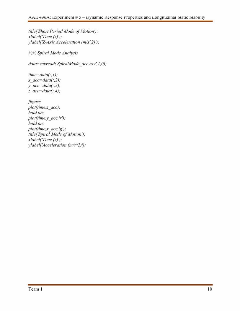
Appendix B—MATLAB Code %% Phugoid Mode Analysis data=csvread('Phugoid_acc.csv',1,0); time=data(:,1); x_acc=data(:,2); y_acc=data(:,3); z_acc=data(:,4); plot(time,z_acc); title('Phugoid Mode of Motion'); xlabel('Time (s)'); ylabel('Z-Axis Acceleration (m/s^2)'); %% Dutch Roll Mode Analysis data=csvread('DutchRoll_acc.csv',1,0); time=data(:,1); x_acc=data(:,2); y_acc=data(:,3); z_acc=data(:,4); figure; plot(time,y_acc,'r'); hold on; plot(time,z_acc); hold on; plot(time,x_acc,'g'); title('Dutch Roll Mode of Motion'); xlabel('Time (s)'); ylabel('Acceleration (m/s^2)'); %% Short Period Mode Analysis data=csvread('ShortPeriod_acc.csv',1,0); time=data(:,1); x_acc=data(:,2); y_acc=data(:,3); z_acc=data(:,4); figure; plot(time,z_acc);


Team 1 10

title('Short Period Mode of Motion'); xlabel('Time (s)'); ylabel('Z-Axis Acceleration (m/s^2)'); %% Spiral Mode Analysis data=csvread('SpiralMode_acc.csv',1,0); time=data(:,1); x_acc=data(:,2); y_acc=data(:,3); z_acc=data(:,4); figure; plot(time,z_acc); hold on; plot(time,y_acc,'r'); hold on; plot(time,x_acc,'g'); title('Spiral Mode of Motion'); xlabel('Time (s)'); ylabel('Acceleration (m/s^2)');


Team 1 11

Appendix C—Control Yoke Relationship

Figure C.1: Deflection Definition

Table C.1: Control Yoke-Elevator Relationship Data


Team 1 12

Figure C.2: Elevator Measurement

Figure C.3: Yoke Measurement


Team 1 13

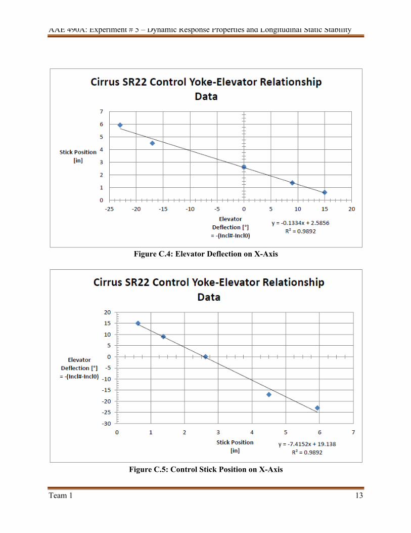
Figure C.4: Elevator Deflection on X-Axis

Figure C.5: Control Stick Position on X-Axis


Team 1 14

Figure C.6: Plot of Table 1

y = -‐0.9295x + 126.81

-‐12

-‐10

-‐8

-‐6

-‐4

-‐2

0 143 143.5 144 144.5 145 145.5 146 146.5 147

delta

E/de

ltaCL (d

egrees)

C.G LocaAon (in)

deltaE/deltaCL vs. CG LocaAon


Team 1 15

Appendix D—Raw Data Cards

Figure D.1: Raw Data Card #1 Dynamic Response Properties


Team 1 16

Figure D.2: Raw Data Card #2 Longitudinal Static Stability

Figure D.3: Raw Data Card #3 Yolk Position vs Elevator Deflection


Team 1 17

Appendix E—Data Reduction

Table E.1: Compiled Data Reduction Table Yoke Position

(in) Elevator

Deflection(deg) Indicated Airspeed

(kts) Altitude(ft) Coefficient of

Lift C.G(in) weight(lbf) 3.06 -3.55 110.00 5000 0.64 145.70 3278.40 3.29 -5.26 100.00 5000 0.78 145.70 3278.40 3.40 -6.07 90.00 5000 0.96 145.70 3278.40 3.14 -4.15 110.00 5000 0.64 145.70 3278.40 3.06 -3.55 120.00 5000 0.54 145.70 3278.40 2.92 -2.51 130.00 5000 0.46 145.70 3278.40 3.50 -6.82 111.00 3000 0.60 146.60 3165.20 3.13 -4.03 101.00 3000 0.73 146.60 3165.20 3.50 -6.82 91.00 3000 0.90 146.60 3165.20 3.00 -3.11 111.00 3000 0.60 146.60 3165.20 2.88 -2.18 120.00 3000 0.50 146.60 3165.20 2.75 -1.25 130.00 3000 0.43 146.60 3165.20 5.06 -18.39 110.00 3500 0.62 146.20 3336.90 5.13 -18.85 100.00 3500 0.75 146.20 3336.90 5.44 -21.17 90.00 3500 0.93 146.20 3336.90 5.06 -18.39 110.00 3500 0.62 146.20 3336.90 4.88 -17.00 120.00 3500 0.52 146.20 3336.90 4.75 -16.07 130.00 3500 0.45 146.20 3336.90 3.19 -4.50 111.00 3000 0.54 144.93 3286.00 3.25 -4.96 101.00 3000 0.66 144.93 3286.00 3.38 -5.89 90.00 3000 0.83 144.93 3286.00 3.19 -4.50 109.00 3000 0.56 144.93 3286.00 3.06 -3.57 120.00 3000 0.46 144.93 3286.00 2.94 -2.64 132.00 3000 0.38 144.93 3286.00

3.125 -4.0345 110 6500 0.67 144.8 3239.8 3.25 -4.9614 100 6500 0.81 144.8 3239.8

3.375 -5.8883 90 6500 0.99 144.8 3239.8 3.125 -4.0345 110 6500 0.67 144.8 3239.8

3 -3.1076 120 6500 0.56 144.8 3239.8 2.875 -2.1807 130 6500 0.48 144.8 3239.8 2.95 -2.7 110 3000 0.8099 143.279 3204.84 3.1 -3.8 100 3000 0.98 143.279 3204.84

3.25 -5 90 3000 1.2099 143.279 3204.84 2.95 -2.7 110 3000 0.8099 143.279 3204.84 2.75 -1.3 120 3000 0.6805 143.279 3204.84 2.6 -0.1 130 3000 0.5799 143.279 3204.84

Documents

Dynamic Response Properties and Longitudinal Static Stability of CIrrus SR22