Embed Size (px)
Citation preview
Hermann Luís Lebkuchen
Dynamic Response and Pitch Damper Designfor a Moderately Flexible, High-Aspect Ratio
Aircraft
Joinville, Brazil
2015
Hermann Luís Lebkuchen
Dynamic Response and Pitch Damper Design for aModerately Flexible, High-Aspect Ratio Aircraft
Trabalho de Conclusão de Curso apresentadocomo requisito parcial para obtenção do título debacharel em Engenharia Aeroespacial no Centrode Engenharias da Mobilidade da UniversidadeFederal de Santa Catarina, Campus de Joinville.
Universidade Federal de Santa Catarina – UFSC
Centro de Engenharias da Mobilidade
Bacharelado em Engenharia Aeroespacial
Supervisor: Prof. Gian Ricardo Berkenbrock, Dr.
Co-supervisor: Alexander Hamann, Dipl.-Ing.
Prof. Robert Luckner, Dr.-Ing.
Joinville, Brazil
2015

Hermann Luís LebkuchenDynamic Response and Pitch Damper Design for a Moderately Flexible, High-Aspect
Ratio Aircraft/ Hermann Luís Lebkuchen. – Joinville, Brazil, 2015-142 p. : il. (algumas color.) ; 30 cm.
Supervisor: Prof. Gian Ricardo Berkenbrock, Dr.
Trabalho de Conclusão de Curso – Universidade Federal de Santa Catarina – UFSCCentro de Engenharias da MobilidadeBacharelado em Engenharia Aeroespacial, 2015.
1. Aeroelasticity. 2.Aeroservoelasticity. 3.Unsteady Aerodynamics. 4.StructuralDynamics. 5.Ground Vibration Tests. 6.Integrated Models. 7.Flight Dynamics. 8.FlightControl. 9. Pitch Damper. I. Supervisor: Prof. Dr. Gian Ricardo Berkenbrock. Co-Supervisor: Dipl.-Ing. Alexander Hamann, Prof. Dr-Ing. Robert Luckner. II. UniversidadeFederal de Santa Catarina. III. Centro de Engenharias da Mobilidade. IV. EngenhariaAeroespacial V. Title: Dynamic Response and Pitch Damper Design for a ModeratelyFlexible, High-Aspect Ratio Aircraft
CDU 02:141:005.7
Hermann Luís Lebkuchen
Dynamic Response and Pitch Damper Design for aModerately Flexible, High-Aspect Ratio Aircraft
Trabalho de Conclusão de Curso apresentadocomo requisito parcial para obtenção do título debacharel em Engenharia Aeroespacial no Centrode Engenharias da Mobilidade da UniversidadeFederal de Santa Catarina, Campus de Joinville.
Trabalho aprovado. Joinville, Brazil, 04 de Dezembro de 2015:
Prof. Gian Ricardo Berkenbrock, Dr.Orientador
Prof. Antônio Otaviano Dourado, Dr.Membro 1
Prof. Rafael Gigena Cuenca, MSc.Membro 2
Joinville, Brazil2015

To my family and all my professors.

Acknowledgements
Firstly, I would like to express my whole-heartedly thanks to my parents that gave mefull support to keep my studies and always motivated me to look forward. Besides that, I wouldlike to express my sincere and special thanks to all of you that in somehow contributed with myeducation and supported me to achieve the development of this work, specially:
• to the fellow students Cassiano Tecchio and Bruno Backes at Universidade Federal deSanta Catarina, where I had the opportunity to daily meet you guys and share interestingideas, specially about computational fluid dynamics and aeroacustics;
• to Prof. Dr.a Viviane Lilian Soethe and Prof. Dr. Gian Ricardo Berkenbrock at UniversidadeFederal de Santa Catarina in Joinville-SC, who in my point of view are an unwaveringexample of kindness and partnership in the relation professor-student;
• to Prof. Dr. Carlos Eduardo de Souza, who advised me during my research about parametersfitting techniques for aeroelastic models at Instituto de Aeronáutica e Espaço in São Josédos Campos-SP and next gave me the opportunity to internship at company AeroEst, wherethe preliminary design of an simplified unmanned aerial vehicle to aeroelastic researchwas carried out;
• to Prof. Dr. Flávio Silvestre, who indicated me to the Institut für Luft- und Raumfahrt atthe Technische Universität Berlin (TU Berlin), Fachgebiet Flugmechanik, Flugregelungund Aeroelastizität (FMRA), where I had the opportunity to know interesting people andto increase my technical skills. I had a great time in Berlin and there I developed the mostpart of this work;
• to Prof. Dr.-Ing. Robert Luckner, Dipl.-Ing. Alexander Hamann and Dipl.-Ing. DavidBieniek at TU Berlin and Prof. Dr.-Ing. Wolf-Reiner Krüger at TU Berlin and also atDeutsches Zentrum für Luft- und Raumfahrt (DLR) in Göttingen. Your orientation, pa-tience, willingness to cooperate and interesting to share your vast knowledge in disciplineslike flight mechanics, flight control, aeroelasticity, aerodynamics, among others was ofgreat importance for me;
At last I acknowledge all of my family, friends, professors and people that directly orindirectly helped me to complete this work and accompanied me though my life. Any omissionin this brief text does not mean lack of gratitude.

"Eppur si muove"
(Galileo Galilei.)
Abstract
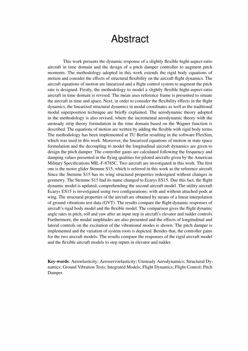
This work presents the dynamic response of a slightly flexible hight-aspect-ratioaircraft in time domain and the design of a pitch damper controller to augment pitchmoments. The methodology adopted in this work extends the rigid body equations ofmotion and consider the effects of structural flexibility on the aircraft flight dynamics. Theaircraft equations of motion are linearized and a flight control system to augment the pitchrate is designed. Firstly, the methodology to model a slightly flexible hight-aspect-ratioaircraft in time domain is revised. The mean axes reference frame is presented to situatethe aircraft in time and space. Next, in order to consider the flexibility effects in the flightdynamics, the linearized structural dynamics in modal coordinates as well as the traditionalmodal superposition technique are briefly explained. The aerodynamic theory adoptedin the methodology is also revised, where the incremental aerodynamic theory with theunsteady strip theory formulation in the time domain based on the Wagner function isdescribed. The equations of motion are written by adding the flexible with rigid body terms.The methodology has been implemented at TU Berlin resulting in the software FlexSim,which was used in this work. Moreover, the linearized equations of motion in state spaceformulation and the decoupling to model the longitudinal aircraft dynamics are given todesign the pitch damper. The controller gains are calculated following the frequency anddamping values presented in the flying qualities for piloted aircrafts given by the AmericanMilitary Specifications MIL-F-8785C. Two aircraft are investigated in this work. The firstone is the motor glider Stemme S15, which is referred in this work as the reference aircraft.Since the Stemme S15 has its wing structural properties redesigned without changes ingeometry. The Stemme S15 had its name changed to Ecarys ES15. Due this fact, the flightdynamic model is updated, comprehending the second aircraft model. The utility aircraftEcarys ES15 is investigated using two configurations: with and without attached pods atwing. The structural properties of the aircraft are obtained by means of a linear interpolationof ground vibrations test data (GVT). The results compare the flight dynamic responses ofaircraft’s rigid body model and the flexible model. The comparison gives the flight dynamicangle rates in pitch, roll and yaw after an input step in aircraft’s elevator and rudder controls.Furthermore, the modal amplitudes are also presented and the effects of longitudinal andlateral controls on the excitation of the vibrational modes is shown. The pitch damper isimplemented and the variation of system roots is depicted. Besides that, the controller gainsfor the two aircraft models. The results compare the responses of the rigid aircraft modeland the flexible aircraft models to step inputs in elevator and rudder.
Key-words: Aeroelasticity; Aeroservoelasticity; Unsteady Aerodynamics; Structural Dy-namics; Ground Vibration Tests; Integrated Models; Flight Dynamics; Flight Control; PitchDamper.

Resumo
O presente trabalho tem como objetivo investigar a resposta dinâmica de umaaeronave moderadamente flexível com alta razão de aspecto no domínio do tempo e projetarum controlador de resposta de arfagem. Primeiramente, a metodologia aplicada nessetrabalho para modelar os efeitos elásticos da aeronave é revisada. O sistema de coordenadasdos eixos médios é apresentado para situar a aeronave no tempo e espaço. Em seguida, asequações de dinâmica estrutural em coordenadas modais bem como a técnica de superposiçãomodal são brevemente revisadas. Na sequência a teoria aerodinâmica incremental comformulação não estacionária baseada na teoria das faixas é apresentada no domínio dotempo com a função de Wagner. O equacionamento apresentado na revisão da metodologiafoi implementado pela TU Berlim no software FlexSim, o qual é utilizado no presentetrabalho com o intuito de automatizar a análise aeroelástica. Ademais, com a linearizaçãodas equações do movimento o sistema de equações é reescrito na forma de espaço de estadose o sistema de controle é apresentado. As equações linearizadas de primeira ordem são entãodesacopladas e reescritas para o movimento longitudinal. A aproximação com dois graus deliberdade para o período curto é dada e um sistema de controle em malha fechada é definido.A frequência e o amortecimento das qualidades de voo requeridas para projetar o controladorsão definidas com base na especificação militar americana MIL-F-8785C. Duas aeronavessão investigadas no trabalho. A primeira aeronave é o motoplanador Stemme S15, que éconsiderado como aeronave de referência, devido ao mesmo ser investigado na literaturapara validação da metodologia utilizada no presente trabalho. A segunda aeronave é a EcarysES15, fruto de modificações nas propriedades estruturais da longarina e da superfície da asada aeronave Stemme S15. Duas configurações da aeronave Ecarys ES15 são investigadas:com e sem pods fixados na parte inferior da asa. As propriedades estruturais da Ecarys ES15são obtidas com ensaios de vibração em solo. Os resultados do ensaio são interpoladoslinearmente sobre toda a geometria da aeronave para consideração dos efeitos elásticos.Os resultados apresentados comparam as respostas dinâmicas das duas aeronaves commodelos de corpo rígido e flexível da estrutura. As variações das velocidades de rolamento,arfagem e guinada são plotadas com comandos no profundor e leme para representar aresposta dinâmica . Além disso, as amplitudes modais são representadas e a relação entre assuperfícies de comando e a excitação de modos de vibração simétricos e não simétricos écomentada. Finalmente, o controlador de resposta de arfagem é implementado e os ganhossão calculados. A influência dos efeitos de flexibilidade nas raízes do sistema de equações,bem como na resposta dinâmica são apresentados e a relevância da consideração dos efeitoselásticos da estrutura é justificada.
Palavras-chaves: Aeroelasticidade; Aeroservoelasticidade; Aerodinâmica não Estacionária;Dinâmica Estrutural; Testes de Vibração em Solo; Modelos Integrados; Dinâmica de Voo;Controle de Voo; Controlador de Arfagem.
List of Figures
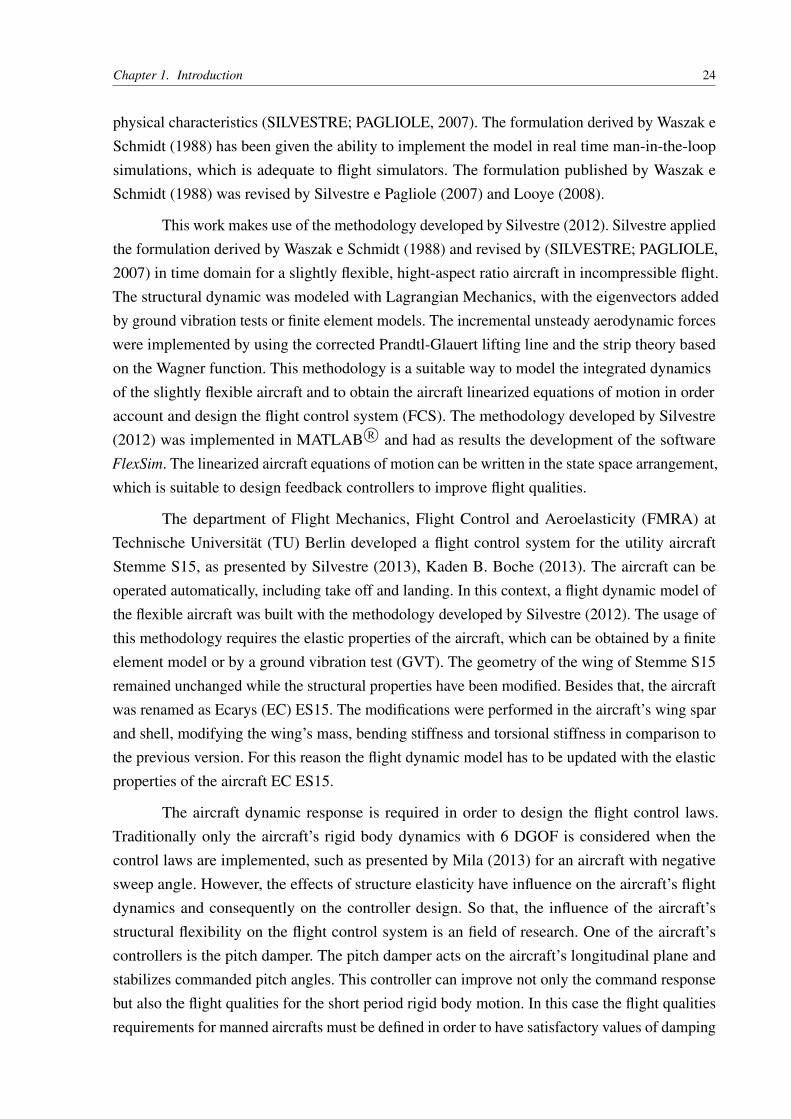
Figure 1 – The aeroelastic triangle of forces with addition of control forces. . . . . . . 23
Figure 2 – Mean axes reference body frame for a slightly flexible aircraft and vectors ofthe wing deformation . . . . . . . . . . . . . . . . . . . . . . . . . . . . . 29
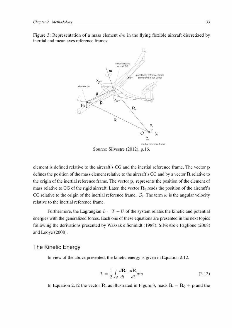
Figure 3 – Representation of a mass element dm in the flying flexible aircraft discretizedby inertial and mean axes reference frames. . . . . . . . . . . . . . . . . . 33
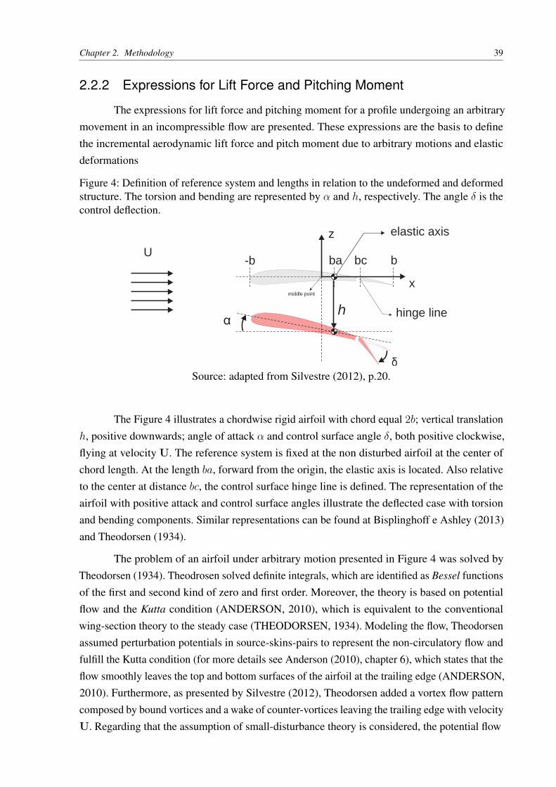
Figure 4 – Definition of reference system and lengths in relation to the undeformed anddeformed structure. The torsion and bending are represented by α and h,respectively. The angle δ is the control deflection. . . . . . . . . . . . . . . 39
Figure 5 – Representation of strip’s geometry and Wagner function versus non-dimensionaltime as an introduction to derivate the unsteady aerodynamic equations for ageneral profile motion with h and α as DGOF. . . . . . . . . . . . . . . . . 44
Figure 6 – Representation of the Duhamel’s integral. Superpositions of infinitesimalangle of attack steps. . . . . . . . . . . . . . . . . . . . . . . . . . . . . . 45
Figure 7 – Representation of forces, moments and velocities associated with the aircraftmotion. . . . . . . . . . . . . . . . . . . . . . . . . . . . . . . . . . . . . . 47
Figure 8 – Behavior of the short period motion with exaggerated effects on attack angleand altitude deviations, and lower damping. . . . . . . . . . . . . . . . . . 48
Figure 9 – Short period frequency requirements for flight phases Category B. . . . . . 52Figure 10 – Block diagram of the pitch damper feedback with the state space aircraft
model and the actuator dynamic block. . . . . . . . . . . . . . . . . . . . . 53
Figure 11 – EC ES15 in flight with pods attached under the wing. . . . . . . . . . . . . 56Figure 12 – Details of the aircraft geometry in three views. . . . . . . . . . . . . . . . . 56Figure 13 – Steps to perform an aeroelastic analysis. . . . . . . . . . . . . . . . . . . . 58Figure 14 – Aircraft’s wing and empennages geometry modeled with strips and lift slopes
representation. . . . . . . . . . . . . . . . . . . . . . . . . . . . . . . . . . 59Figure 15 – Aircraft EC ES15 at GVT tests performed at the company Leichtwerk in
Braunschweig, Germany. . . . . . . . . . . . . . . . . . . . . . . . . . . . 61Figure 16 – Motor glider EC ES15 with pods attached under the both sides of the wing. . 61Figure 17 – Motor glider EC ES15 without attached pods. . . . . . . . . . . . . . . . . 63Figure 18 – Concentrated points containing the ground vibration tests’ results interpolated
at three-quarter chord for wing and empennages. . . . . . . . . . . . . . . . 64Figure 19 – Interpolation steps performed to represent the structural dynamic over the
aircraft geometry. . . . . . . . . . . . . . . . . . . . . . . . . . . . . . . . 65
Figure 20 – Two dimensional representation of undeformed and deformed wing pro-file with pitching, plunging and lagging components to perform the linearinterpolation of modal shapes. . . . . . . . . . . . . . . . . . . . . . . . . . 66
Figure 21 – Representation of the first asymmetric wing torsion of EC ES15 aircraft, withmodal frequency equal 29.10Hz. . . . . . . . . . . . . . . . . . . . . . . . 67
Figure 22 – Stationary deformation at trimmed flight condition established in Table 9 foraircraft EC ES15, configuration without pods. . . . . . . . . . . . . . . . . 71
Figure 23 – Flight Simulation results for aircraft Stemme S15 with 1o elevator command. 72Figure 24 – Flight Simulation results for aircraft Stemme S15 with 1o rudder command. 72Figure 25 – Modal Amplitudes for the aircraft Stemme S15. . . . . . . . . . . . . . . . 73Figure 26 – Flight Simulation results for aircraft EC ES15 without pods with1o elevator
command. . . . . . . . . . . . . . . . . . . . . . . . . . . . . . . . . . . . 74Figure 27 – Flight Simulation results for EC ES15 without pods with rudder command. . 74Figure 28 – Flight Simulation Results for EC ES15 without pods with rudder command. 75Figure 29 – Flight Simulation results for EC ES15 with pods and rudder step command. 76Figure 30 – Flight Simulation Results for EC ES15 without pods with rudder command. 76Figure 31 – Longitudinal motion approximation for the aircraft Stemme S15. Representa-
tion of the short period and phugoid roots for the rigid and flexible modelswith and without the controller action. . . . . . . . . . . . . . . . . . . . . 79
Figure 32 – Longitudinal motion approximation for the aircraft EC ES15 without pods.Representation of the short period and phugoid roots for the rigid and flexiblemodels with and without the controller action. . . . . . . . . . . . . . . . . 80
Figure 33 – ECARY ES15 with pods root loci. . . . . . . . . . . . . . . . . . . . . . . 81Figure 34 – Step input of 1o in the elevator command ηcmd and the tracking error signal ηe. 82Figure 35 – Short period (SP) approximation. Step input of 1o in elevator command. The
pitch rate and attack angle state vectors are illustrated for the rigid and flexiblestructural models. The dashed lines display the open loop (OL) and the fulllines the closed loop (CL) control system. . . . . . . . . . . . . . . . . . . 83
Figure 36 – Longitudinal Motion (LB) approximation. Step input of 1o in elevator com-mand. The pitch rate and attack angle state vectors are illustrated for the rigidand flexible structural models. The dashed lines display the open loop (OL)and the full lines the closed loop (CL) control system. . . . . . . . . . . . . 84
Figure 37 – Longitudinal Motion (LB) approximation. Step input of 1o in elevator com-mand. The pitch rate and attack angle state vectors are illustrated for the rigidand flexible structural models. The dashed lines display the open loop (OL)and the full lines the closed loop (CL) control system. . . . . . . . . . . . . 85
Figure 38 – Step input of 1o in elevator command. Pitch rate response of the three aircraftmodels for open loop (OL) and closed loop (CL) control system. Comparisonbetween rigid model and flexible models. . . . . . . . . . . . . . . . . . . . 85
Figure 39 – Step input of 1o in elevator command. Attack angle response of the threeaircraft models for open loop (OL) and closed loop (CL) control system.Comparison between rigid model and flexible models. . . . . . . . . . . . . 86
Figure 74 – Short period (SP) approximation. Step input of 1o in elevator command. Pitchrate and attack angle variations for rigid and flexible structural models. Thedashed lines display the open loop (OL) and the full lines the closed loop(CL) control system. Simulation time 5s. . . . . . . . . . . . . . . . . . . . 106
Figure 75 – Longitudinal Motion (LB) approximation. Step input of 1o in elevator com-mand. Pitch rate and attack angle variations for rigid and flexible structuralmodels. The dashed lines display the open loop (OL) and the full lines theclosed loop (CL) control system. Simulation time 5s. . . . . . . . . . . . . 107
Figure 76 – Longitudinal Motion (LB) approximation. Step input of 1o in elevator com-mand. Pitch rate and attack angle variations for rigid and flexible structuralmodels. The dashed lines display the open loop (OL) and the full lines theclosed loop (CL) control system. Simulation time 20s. . . . . . . . . . . . . 107
Figure 77 – Longitudinal Motion (LB) approximation. Step input of 1o in elevator com-mand. Pitch rate and attack angle variations for rigid and flexible structuralmodels. The dashed lines display the open loop (OL) and the full lines theclosed loop (CL) control system. Simulation time 400s. . . . . . . . . . . . 108
Figure 78 – Short period (SP) approximation. Step input of 1o in elevator command. Pitchrate and attack angle variations for rigid and flexible structural models. Thedashed lines display the open loop (OL) and the full lines the closed loop(CL) control system. Simulation time 5s. . . . . . . . . . . . . . . . . . . . 108
Figure 79 – Longitudinal Motion (LB) approximation. Step input of 1o in elevator com-mand. Pitch rate and attack angle variations for rigid and flexible structuralmodels. The dashed lines display the open loop (OL) and the full lines theclosed loop (CL) control system. Simulation time 5s. . . . . . . . . . . . . 109
Figure 80 – Longitudinal Motion (LB) approximation. Step input of 1o in elevator com-mand. Pitch rate and attack angle variations for rigid and flexible structuralmodels. The dashed lines display the open loop (OL) and the full lines theclosed loop (CL) control system. Simulation time 20s. . . . . . . . . . . . . 109
Figure 81 – Longitudinal Motion (LB) approximation. Step input of 1o in elevator com-mand. Pitch rate and attack angle variations for rigid and flexible structuralmodels. The dashed lines display the open loop (OL) and the full lines theclosed loop (CL) control system. Simulation time 400s. . . . . . . . . . . . 110
Figure 82 – Open loop block diagram implemented in MATLAB R© Simulink. . . . . . . 134Figure 83 – Closed loop block diagram implemented in MATLAB R© Simulink. . . . . . 134
List of Tables
Table 1 – Operational flight envelopes. . . . . . . . . . . . . . . . . . . . . . . . . . . 51Table 2 – Short period mode damping. . . . . . . . . . . . . . . . . . . . . . . . . . . 52Table 3 – Short period damping and frequency ratio limits for an aircraft with flight
phase Category B and Level 1. . . . . . . . . . . . . . . . . . . . . . . . . . 53
Table 4 – EC ES15 general properties. . . . . . . . . . . . . . . . . . . . . . . . . . . 57Table 5 – Structural properties of Stemme S15. . . . . . . . . . . . . . . . . . . . . . 60Table 6 – Structural properties of EC ES15 with pods. . . . . . . . . . . . . . . . . . . 62Table 7 – Structural properties of EC ES15 without pods. . . . . . . . . . . . . . . . . 63Table 8 – Definition of flying qualities for the utility aircraft EC ES15 following (MIL-
F-8785C, 1980). . . . . . . . . . . . . . . . . . . . . . . . . . . . . . . . . 67
Table 9 – Reference condition to trimmed flight. . . . . . . . . . . . . . . . . . . . . . 68Table 10 – Values of trim parameters with reference flight at 44m/s and retracted flaps. . 69Table 11 – Values of trim parameters with reference flight at 44m/s and retracted flaps. . 70Table 12 – Pitch damper results for the reference aircraft Stemme S15. . . . . . . . . . . 78Table 13 – Pitch damper results for the reference aircraft EC ES15 without pods. . . . . 79Table 14 – Pitch damper results for the reference aircraft EC ES15 with pods. . . . . . . 80Table 15 – Pitch damper controller gains. . . . . . . . . . . . . . . . . . . . . . . . . . 81Table 16 – Steady values of aircraft models given in Figures 38 and 39. . . . . . . . . . 86Table 17 – Differences between the rigid and flexible structural models in percentage. . . 86
List of abbreviations and acronyms
MIL United States Military Standard
FAA Federal Aviation Administration
TUB Technische Universität Berlin
FMRA Fachgebiet Flugmechanik, Flugregelung und Aeroelastizität
EC Ecarys
CG Center of Gravity
CM Center of Mass
MATLAB Matrix Laboratory
MAC Mean aerodynamic chord
GVT Ground Vibration Test
EMA Experimental Modal Analysis
OMA Operational Modal Analysis
FEM Finite Element Model
FCS Flight Control System
DGOF Degrees of Freedom
EOM Equations of Motion
LAPAZ Luft-Arbeits-Plattform-für-die-Allgemeine-Zivilluftfahrt
EFRE Europäischer Fonds für regionale Entwicklung
TAS True air speed
CFD Computational Fluid Dynamics
SAC Structure-Aerodynamic Coupling
TUHH Technische Universität Hamburg-Harburg
HTP Horizontal tail plane
VTP Vertial tail plane
CAD Computer Aided Design
CR Cruise Flight
RB Rigid-body
S Symmetric
A Asymmetric

List of symbols
Latin Characters:
a number of degrees of freedom of the discrete structural system
A system’s matrix in state space formulation
Amod modified system’s matrix in state space formulation due to feedback control
b half wing span
b in chapter 2, also used as half airfoil’s length
B system’s input matrix in state space formulation
c airfoil’s chord
c mean aerodynamic chord
C(k) Theodorsen’s function (k means reduced frequency)
C origin of the fixed reference frame in chapter 2
C system’s output matrix in state space formulation
Drigid aerodynamic drag in subsection 2.1.3
D structural damping matrix
D system’s feedforward matrix in state space formulation
D dissipation function
dm differential element of mass
H flight altitude
Hoperational aircraft’s operational ceiling
Ix, Iy, Iz moments of inertia in roll, pitch and yaw axis
Iyz, Ixz, Ixy products of inertial in roll, pitch and yaw axis
J inertia tensor
j imaginary unity,√−1
K stiffness matrix
k reduced frequency in chapter 2
k also used in index as counter
kηq controller gain from elevator to pitch rate in pitch damper design
kηα controller gain from elevator to attack angle in pitch damper design
Lrigid used in Equation 2.37 as lift force
L Lagrangian, L = T − U
L,M,N used in chapter 3 as the aerodynamic moment components in roll, pitch andyaw axis
L used in section 3.2 as the aircraft’s fuselage length
`C circulatory portion of lift per unit span
`NC non circulatory portion of lift per unit span
M mass matrix
m aircraft’s mass in chapter 3
m in chapter 2 used as profile’s pitching moment per unit span
mC circulatory airfoil’s pitching moment per unit span at elastic axis
mNC non circulatory airfoil’s pitching moment per unit span at elastic axis
mempty aircraft’s mass in empty configuration
mPL aircraft’s payload mass
mtotal aircraft’s mass full filled
nα aircraft’s load factor response to attack angle in g’s per radian
ne used as number of chosen elastic modes
Ol origin of the inertial reference frame
OM origin of the mean axes reference frame
p position vector of a structural element dm relative to the origin of the bodyreference frame
pd elastic displacement of the mass element dm

p, q, r roll, pitch and yaw angular rates
pr position of the mass element dm of the undeformed structure in relation tothe point C and elastic displacement pd
q vector of the physical coordinates of the discrete elastic system
Qrigid used in Equation 2.37 as aerodynamic force in z−direction
Q in chapter 2 used for the downwash at the profile’s 3/4−chord position
Qη vector of generalized forces on the elastic DGOF
R position vector of the origin of the lifting surface’s local body coordinatesystem relative to the aircraft CG
R0 position of the aircraft centre of gravity relative to the origin of the inertialreference frame
rM distance between the origin of the fixed and the floating reference frames
S reference wing’s area
s non dimensional time defined in semi-chord traveled lengths
S(K) Sear’s function
t time
T kinetic energy in subsection 2.1.3
T
u, v, w used in chapter 2 as the velocity components in roll, pitch and yaw axis
u system’s input or control vector
U undisturbed flow velocity
UG gravitational potential energy
US deformation energy
V flight velocity in section 2.3
VTAS true air speed
V aircraft’s volume
w3/4 x -position of the three-quarter-chord point on the local body reference frame
X, Y, Z aerodynamic force components
x system’s state vector in state space formulation
x system’s derivative of the vector with respect to time in state space formula-tion
y system’s output vector in state space formulation
Greek Characters
α angle of attack
β sideslip angle
β modal structural damping matrix
δ control deflection in section 2.2
ε strain tensor
η elevator command surface
ηe tracking error
ηF thrust command
ηk flaps command
η column vector of modal amplitudes, [η1,η2,η3, . . . ,ηne]T
η vector of modal amplitudes
ηk amplitude of the k-th elastic modal shape
γ modal stiffness matrix
Λ eigenvector matrix of the undamped structural eigenvalue problem
Λ matrix of eigenvectors of the ne chosen elastic modes
µ modal mass matrix
ω aircraft angular velocity vector relative to the aircraft CG
ωC/M angular velocity of the reference frame fixed on the undeformed structurerelative to the mean axes
ωnk natural frequency of the k-th elastic mode
ωnPH phugoid frequency
ωnSP short period frequency
ω∗nSP modified short period frequency (with pitch damper)
ψ, θ, φ Euler’s angles from yaw, pitch and roll
Φ Wagner’s Function
Φ matrix of elastic modal shapes
Φ matrix of modal shapes of the ne chosen elastic mode
σ stress tensor
ξ aileron command
ζ rudder command
ζnk k−th damping of the undamped structural eigenvalue
ζPH phugoid damping
ζSP short period damping
ζ∗PH modified phugoid damping
ζ∗SP modified short period damping
Contents
1 Introduction . . . . . . . . . . . . . . . . . . . . . . . . . . . . . . . . . . . . 221.1 Contextualization . . . . . . . . . . . . . . . . . . . . . . . . . . . . . . . . . 221.2 Objective . . . . . . . . . . . . . . . . . . . . . . . . . . . . . . . . . . . . . 251.3 Overview . . . . . . . . . . . . . . . . . . . . . . . . . . . . . . . . . . . . . 25
2 Methodology . . . . . . . . . . . . . . . . . . . . . . . . . . . . . . . . . . . . 272.1 Equations of Motion of Slightly Flexible Aircraft . . . . . . . . . . . . . . . . 27
2.1.1 Mean Axes Reference Frame . . . . . . . . . . . . . . . . . . . . . . . 272.1.2 Structural Dynamics . . . . . . . . . . . . . . . . . . . . . . . . . . . 292.1.3 Elastic Airplane Equations of Motion . . . . . . . . . . . . . . . . . . 32
2.2 Unsteady Incremental Aerodynamics in Incompressible Flow . . . . . . . . . . 382.2.1 Foreword to Unsteady Incremental Aerodynamics Theory . . . . . . . . 382.2.2 Expressions for Lift Force and Pitching Moment . . . . . . . . . . . . 392.2.3 Classical Problems Involving Incremental Aerodynamics . . . . . . . . 412.2.4 Incremental Aerodynamic Derivatives for an Arbitrary Motion . . . . . 43
2.3 Flight Control System . . . . . . . . . . . . . . . . . . . . . . . . . . . . . . . 472.3.1 Longitudinal Dynamics . . . . . . . . . . . . . . . . . . . . . . . . . . 472.3.2 State Space Formulation . . . . . . . . . . . . . . . . . . . . . . . . . 482.3.3 Flying Qualities Requirements . . . . . . . . . . . . . . . . . . . . . . 502.3.4 Pitch Damper Implementation . . . . . . . . . . . . . . . . . . . . . . 53
3 Models . . . . . . . . . . . . . . . . . . . . . . . . . . . . . . . . . . . . . . . 553.1 Flight Simulation Model . . . . . . . . . . . . . . . . . . . . . . . . . . . . . 553.2 Aircraft . . . . . . . . . . . . . . . . . . . . . . . . . . . . . . . . . . . . . . 553.3 Aeroelastic Model . . . . . . . . . . . . . . . . . . . . . . . . . . . . . . . . . 57
3.3.1 Structural Properties . . . . . . . . . . . . . . . . . . . . . . . . . . . 593.3.1.1 Stemme S15 . . . . . . . . . . . . . . . . . . . . . . . . . . 603.3.1.2 Ecarys ES15 . . . . . . . . . . . . . . . . . . . . . . . . . . 60
3.3.2 Linear Interpolation of Modal Shapes from Ground Vibration Test . . . 643.4 Definition of Flying Qualities Requirements . . . . . . . . . . . . . . . . . . . 66
4 Results and Discussion . . . . . . . . . . . . . . . . . . . . . . . . . . . . . 684.1 Effects of Structural Flexibility . . . . . . . . . . . . . . . . . . . . . . . . . . 684.2 Simulation of Aircraft Flight Dynamics . . . . . . . . . . . . . . . . . . . . . 714.3 Pitch Damper . . . . . . . . . . . . . . . . . . . . . . . . . . . . . . . . . . . 77
4.3.1 Assumptions . . . . . . . . . . . . . . . . . . . . . . . . . . . . . . . 77

4.3.2 System Roots . . . . . . . . . . . . . . . . . . . . . . . . . . . . . . . 774.3.3 Pitch Damper Results . . . . . . . . . . . . . . . . . . . . . . . . . . . 81
5 Conclusions and Final Remarks . . . . . . . . . . . . . . . . . . . . . . . . 875.1 Final Remarks . . . . . . . . . . . . . . . . . . . . . . . . . . . . . . . . . . . 895.2 Future Works . . . . . . . . . . . . . . . . . . . . . . . . . . . . . . . . . . . 89
Bibliography . . . . . . . . . . . . . . . . . . . . . . . . . . . . . . . . . . . . . . 91
Appendix 95
APPENDIX A Modal Shapes of Models . . . . . . . . . . . . . . . . . . . . . 96A.1 Stemme S15 . . . . . . . . . . . . . . . . . . . . . . . . . . . . . . . . . . . . 96A.2 Ecarys ES15 without PODs . . . . . . . . . . . . . . . . . . . . . . . . . . . . 99A.3 Ecarys ES15 with PODs . . . . . . . . . . . . . . . . . . . . . . . . . . . . . 102
APPENDIX B Pitch Damper Results . . . . . . . . . . . . . . . . . . . . . . . 106B.1 Stemme S15 . . . . . . . . . . . . . . . . . . . . . . . . . . . . . . . . . . . . 106B.2 Ecarys ES15 with pods . . . . . . . . . . . . . . . . . . . . . . . . . . . . . . 108
APPENDIX C Implemented Algorithms . . . . . . . . . . . . . . . . . . . . . 111C.1 mfv2StructFlexSimInput.m . . . . . . . . . . . . . . . . . . . . . . . . . . . . 111
C.1.1 InterpStreifenGVT.m . . . . . . . . . . . . . . . . . . . . . . . . . . . 112C.1.2 ReadGVTData.m . . . . . . . . . . . . . . . . . . . . . . . . . . . . . 122
C.2 pitch_damper.m . . . . . . . . . . . . . . . . . . . . . . . . . . . . . . . . . . 134
22
1 Introduction
1.1 Contextualization
The design of an aircraft is a complex iterative task that involves requirements, sizing,trade studies and analysis to end up with a final concept (CHIOZZOTTO, 2013). Diverse groupswork together in order to design all necessary systems to assure that a flight vehicle is capableto fulfill the requirements and perform its flight envelope without compromise safety factors.Among all fields involved into the aircraft design, the disciplines of propulsion, avionics, flighttests, control, aerodynamic and structures work together to find the best design solution available.One of the disciplines that came up as a source of problems in moder aircraft design is theaeroelasticity (DOWELL, 2014).
As defined in Bisplinghoff e Ashley (2013) the aeroelasticity is the discipline thatinvolves the interaction between aerodynamic, inertial and elastic forces. Besides that, if theairplane structure were perfectly rigid, no aeroelastic problems would exist. Modern flight vehiclestructures are in most cases very flexible, which is the source of aeroelastic problems. One ofthe first documented aeroelastic problem in airplane design, according to Bisplinghoff e Ashley(2013) and Fung (2002), dates from the World War I with the biplane military bomber HandleyPage 0/400. This aircraft experienced violent oscillations at fuselage and tail surfaces. Afterthat, with the development of the monoplane wing Fokker D-8, problems involving the aircraft’swing like torsion-bending divergence and flutter, loss of aileron effectiveness and changes inload distribution were experienced. With the development of aeronautic industry, the flight speedwas increased and aeroelastic problems were even more evidenced, creating the necessity tobetter understand what kind of physical effects were happening. In the aircraft design history, theaeroelastic phenomenon raised in the aeronautic history as a source of problem (SILVESTRE,2012). Livne (2003) states that nowadays the consideration of aeroelasticity since the first stepsof the aircraft design can bring many benefits like costs reduction, performance improvements,lower weight structures and the ability to explore new concepts.
Collar (1946) represented the aeroelastic phenomena by means of a triangle. Each vertexof this triangle illustrates one of the forces related with aeroelastic phenomena. The forces are:aerodynamic, inertial and elastic. The representation of aeroelasticity by means of the Collar’sdiagram displays not only static but also dynamic problems. The classical Collar’s diagram,presented in Figure 1, can be also expanded to a pyramid in order to account for control forces,in this case the aeroelasticity is commonly defined as aeroservoelasticity (WRIGHT; COOPER,2015). Barbarino et al. (2011) and Silvestre e Pagliole (2007) state that during the last decades ofaeronautic research development, the flexibility of structures has been increased due the adoptionof new materials and multidisciplinary optimization methods, such as composites in association
Chapter 1. Introduction 23
with tailoring techniques, in order to design lighter and strengthen structures. Furthermore,since the flexibility effects may also change the aircraft geometry and consequently the loadsdistributions, to consider the effects of flexibility into the flight mechanics and control designbecomes a substantial task (LOOYE, 2008).
Figure 1: The aeroelastic triangle of forces with addition of control forces.
AerodynamicForces
InertialForces
ControlForces
ElasticForces
Static Aeroelasticity
Vibrations
Flight MechanicsDynamic Aeroelasticity
Source: Adapted from (WRIGHT; COOPER, 2015), pg 20 and 202.
Traditionally, the flight mechanics and aeroelasticity are treated aside of each other aspresented in Etkin e Reid (1998) and Nelson (1998) for applications to performance, handlingqualities and control analysis. For this case, the airplane is assumed as a rigid-body, withoutconsideration of elastic degrees of freedom (DGOF). However, when the structure has significanteffects of flexibility, the rigid body frequencies get closer to the frequencies of the elastic DGOF,so that the difference between frequencies of rigid-body and elastic modes is reduced (WASZAK;SCHMIDT, 1988).
The interaction between aeroelasticity and flight mechanics is implemented through theaerodynamic loading and mass distribution. When the aircraft perform dynamic maneuvers, theaerodynamic loading change due to the structural displacements in the volume, modifying themass distribution and consequently the center of gravity (CG) and moments of inertia. The alter-ation of aircraft’s CG position and moment of inertia modify the aircraft flight dynamic response(WASZAK; DAVIDSON; SCHMIDT, 1987a). The usage of integrated models represents anextension of the rigid body dynamics with the consideration of structural flexibility and massdistributions effects. Milne (1968) started the investigation of flight dynamics of aeroelastic vehi-cles considering three DGOF, after that CAVIN III e Dusto (1977) used the mean axes referencesframe to derive the equations of motion of a flexible aircraft using Lagrangian Mechanics, wherethe structure was represented with finite element models. Moreover, Waszak, Davidson e Schmidt(1987a) and Waszak, Davidson e Schmidt (1987b) simplified the expressions working with thelinearized mean axes considering small displacement of the structure. The consideration of smalldisplacements means that the structure displacements are much smaller than the displacement ofthe aircraft’s center of gravity and the linear structural dynamics can be used without losing real
Chapter 1. Introduction 24
physical characteristics (SILVESTRE; PAGLIOLE, 2007). The formulation derived by Waszak eSchmidt (1988) has been given the ability to implement the model in real time man-in-the-loopsimulations, which is adequate to flight simulators. The formulation published by Waszak eSchmidt (1988) was revised by Silvestre e Pagliole (2007) and Looye (2008).
This work makes use of the methodology developed by Silvestre (2012). Silvestre appliedthe formulation derived by Waszak e Schmidt (1988) and revised by (SILVESTRE; PAGLIOLE,2007) in time domain for a slightly flexible, hight-aspect ratio aircraft in incompressible flight.The structural dynamic was modeled with Lagrangian Mechanics, with the eigenvectors addedby ground vibration tests or finite element models. The incremental unsteady aerodynamic forceswere implemented by using the corrected Prandtl-Glauert lifting line and the strip theory basedon the Wagner function. This methodology is a suitable way to model the integrated dynamicsof the slightly flexible aircraft and to obtain the aircraft linearized equations of motion in orderaccount and design the flight control system (FCS). The methodology developed by Silvestre(2012) was implemented in MATLAB R© and had as results the development of the softwareFlexSim. The linearized aircraft equations of motion can be written in the state space arrangement,which is suitable to design feedback controllers to improve flight qualities.
The department of Flight Mechanics, Flight Control and Aeroelasticity (FMRA) atTechnische Universität (TU) Berlin developed a flight control system for the utility aircraftStemme S15, as presented by Silvestre (2013), Kaden B. Boche (2013). The aircraft can beoperated automatically, including take off and landing. In this context, a flight dynamic model ofthe flexible aircraft was built with the methodology developed by Silvestre (2012). The usage ofthis methodology requires the elastic properties of the aircraft, which can be obtained by a finiteelement model or by a ground vibration test (GVT). The geometry of the wing of Stemme S15remained unchanged while the structural properties have been modified. Besides that, the aircraftwas renamed as Ecarys (EC) ES15. The modifications were performed in the aircraft’s wing sparand shell, modifying the wing’s mass, bending stiffness and torsional stiffness in comparison tothe previous version. For this reason the flight dynamic model has to be updated with the elasticproperties of the aircraft EC ES15.
The aircraft dynamic response is required in order to design the flight control laws.Traditionally only the aircraft’s rigid body dynamics with 6 DGOF is considered when thecontrol laws are implemented, such as presented by Mila (2013) for an aircraft with negativesweep angle. However, the effects of structure elasticity have influence on the aircraft’s flightdynamics and consequently on the controller design. So that, the influence of the aircraft’sstructural flexibility on the flight control system is an field of research. One of the aircraft’scontrollers is the pitch damper. The pitch damper acts on the aircraft’s longitudinal plane andstabilizes commanded pitch angles. This controller can improve not only the command responsebut also the flight qualities for the short period rigid body motion. In this case the flight qualitiesrequirements for manned aircrafts must be defined in order to have satisfactory values of damping
Chapter 1. Introduction 25
and frequency.
1.2 Objective
In face of the concepts of aeroelasticity and aeroservoelasticity, the importance to considerthe structural flexibility effects into the aircraft flight mechanics and the new wing structuralproperties of the utility aircraft presented above, the general objective of this work is given asfollows:
General Objectives
• Update of the existing flight dynamic model developed at TU Berlin with the properties ofthe aircraft EC ES15 using the in-house software FlexSim. Furthermore, a pitch dampershall be designed to augment the short period of the EC ES15;
Based on the main objectives, the specific objectives are presented in the following.
Specific Objectives
• Literature study on the subjects of flight dynamic model of elastic aircrafts, flying qualitiesand flight control systems;
• Transformation of the GVT eigenvectors and eigenvalues into structural input data forFlexSim. With the aircraft structural behavior and the aerodynamic strip models, the flightdynamics shall be simulated with the in-house FlexSim and the rigid body and flexiblemodels response of the EC ES15 and the Stemme S15 compared;
• The definition of the damping and frequency for the pitch damper shall follow the flightquality requirements given in MIL-F-8785C (1980) for the short period motion. Analgorithm that computes pitch damper parameters for adjusting the flight dynamic charac-teristics according to the requirements shall be implemented. The controller augmentationshall be compared for the rigid and flexible aircraft;
1.3 Overview
The structure of this work is depicted as follows:
• chapter 2 - Methodology:
– Equations of Motion of Slightly Flexible Aircraft: First, the representation of theaircraft in time and space by means of the mean references axes is introduced, next the
Chapter 1. Introduction 26
classic modal superposition technique for structural dynamics is presented. Further,the elastic equations of motion are written with Lagrangian mechanics, which relatesthe kinetic and potential energies with the generalized forces.
– Unsteady Aerodynamic: The incremental unsteady aerodynamic based on the poten-tial theory is shortly presented. The lift force and pitch moment expressions for aprofile undergoing arbitrary motion in incompressible flow, the use of Theodorsen,Wagner and Küssner functions are also briefly introduced;
– Flight Control System (FCS): The linearized equations of motion in state-spaceformulation are given. The system’s matrix, system’s input matrix, output state vectorwith longitudinal and lateral motion properties and control vector are defined. Thelongitudinal approximation and rigid-body characteristic motions are introduced.The short period approximation as well as the aircraft’s flight dynamic qualities andthe pitch damper implementation are later presented;
• chapter 3 - Models:
– Flight Simulation Model: Briefly introduction about the non-linear high-fidelity flightsimulation model developed at TU Berlin with MATLAB R© Simulink for the utilityaircraft Stemme S15;
– Aircraft: General properties of the aircraft EC ES15.
– Aeroelastic Model: Both structural properties of the aircraft Stemme S15 and ECES15 with and without pods are given.
– Linear interpolation of modal shapes from ground vibration tests (GVT) data and theconstruction of the readable input file to FlexSim are carried out;
• chapter 4 - Results and Discussion:
– Flight dynamic response: The effects of structural flexibility are presented for thestationary trimmed flight. Next, the flight dynamic response of the aircrafts StemmeS15 and EC ES15 with and without pods are compared presenting the pitch rates ofthe rigid body and flexible structural modes for a step input of1o in the elevator andrudder. Furthermore, the modal amplitudes and changes in altitude are also presented;
– Pitch damper: The frequency and damping are defined and the the equations ofmotion to longitudinal and short period approximations are depicted. The pitchdamper results are given comparing the aircraft models with rigid body and flexiblestructural properties; and
• chapter 5 - Conclusions:
– The conclusions achieved with the development of this work are presented, followedby final remarks and the proposed future works.
27
2 Methodology
This work applies the methodology developed by Silvestre (2012) with the objectiveto simulate the dynamics of slightly flexible, hight-aspect-ratio aircraft in the time domain.The subsection 2.1.1 introduces the mean axes reference frame to situate the aircraft in timeand space. Further in subsection 2.1.2, the linear structural dynamics in the modal coordinatesfollowed by the Lagrangian Mechanics are introduced. Based on the floating reference frame andmodal coordinates, the equations of motion of flexible aircraft are presented in subsection 2.1.3.Next, the section 2.2 depicts the unsteady incremental aerodynamic formulation to consider thechanges in loads caused by structure deformations. In subsection 2.3.4 the linearized equations ofmotion in state space formulation are introduced. The desired damping and frequency followingthe military flight qualities MIL-F-8785C are given according to the aircraft’s flight phase, levelof flight and flight envelope. Further, the pitch damper implementation is carried out with thelongitudinal and short period approximations.
2.1 Equations of Motion of Slightly Flexible Aircraft
2.1.1 Mean Axes Reference Frame
Before starting to derive the aircraft differential equations of motion, it is first necessaryto define an appropriate and secure foundation on which to build the models. The foundationmeans a mathematical framework where the equations of motion can be developed in order torepresent the aircraft in time and space (COOK, 2012). In flight mechanics literature such asEtkin e Reid (1998) and Hull (2007), the aircraft is modeled as a rigid body with fixed engines, anaft tail and a right-left plane of symmetry. With such model the diagram of forces in symmetricflight comprehend in thrust, lift, drag and weight acting at the aircraft center of gravity (CG).This type of reference frame is called "fixed reference frame".
The approach of rigid body is suitable when the elastic effects are not significant for theanalysis or the structure has high stiffness properties. However, when the structural displacementschange the aircraft volume V , and consequently its center of gravity and moment of inertia, theflight dynamic response is affected (SILVESTRE; PAGLIOLE, 2007). Thus, the consideration offlexibility effects on the aircraft’s dynamic response becomes an important issue. Assuming theaircraft as an elastic body, it changes its form due loads during the flight and the concept of bodyreference frame must be extended. Waszak e Schmidt (1988) assert that " during the process of
developing equations of motion of any unconstrained elastic system, inertial coupling can occur
between the rigid-body degrees of freedom (DGOF) and the elastic DGOF unless a appropriate
choice for the local body-reference coordinate is used". In this case, the body reference frame is
Chapter 2. Methodology 28
not essentially defined with a fixed point but can also have a relative motion in relation to theCG. These words define the "floating reference frame".
Different body reference frames were defined such as the mean axes reference frame,the principal axes reference frame, the body reference frame fixed on a physical point of thedeformable body, among others (SILVESTRE, 2012). The methodology applied in this workmakes use of the mean axes reference frame. The justification of the use of this reference systemis that it simplifies significantly the kinetic energy expression in Lagrange equations, which aregoing to be present further in subsection 2.1.2.
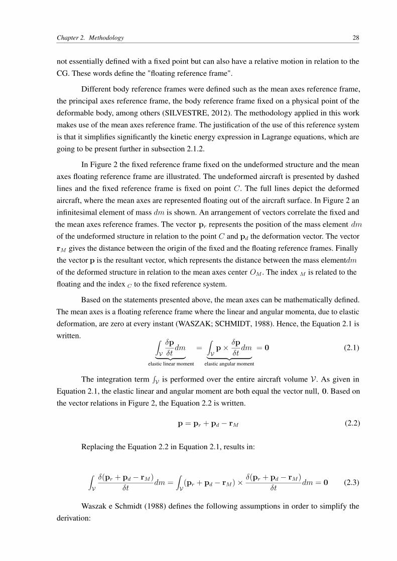
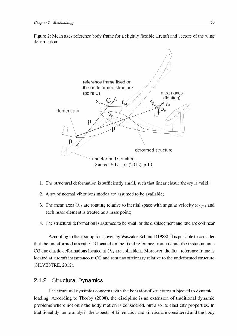
In Figure 2 the fixed reference frame fixed on the undeformed structure and the meanaxes floating reference frame are illustrated. The undeformed aircraft is presented by dashedlines and the fixed reference frame is fixed on point C. The full lines depict the deformedaircraft, where the mean axes are represented floating out of the aircraft surface. In Figure 2 aninfinitesimal element of mass dm is shown. An arrangement of vectors correlate the fixed andthe mean axes reference frames. The vector pr represents the position of the mass element dmof the undeformed structure in relation to the point C and pd the deformation vector. The vectorrM gives the distance between the origin of the fixed and the floating reference frames. Finallythe vector p is the resultant vector, which represents the distance between the mass elementdmof the deformed structure in relation to the mean axes center OM . The index M is related to thefloating and the index C to the fixed reference system.
Based on the statements presented above, the mean axes can be mathematically defined.The mean axes is a floating reference frame where the linear and angular momenta, due to elasticdeformation, are zero at every instant (WASZAK; SCHMIDT, 1988). Hence, the Equation 2.1 iswritten. ∫
V
δpδtdm︸ ︷︷ ︸
elastic linear moment
=∫V
p× δpδtdm︸ ︷︷ ︸
elastic angular moment
= 0 (2.1)
The integration term∫V is performed over the entire aircraft volume V . As given in
Equation 2.1, the elastic linear and angular moment are both equal the vector null, 0. Based onthe vector relations in Figure 2, the Equation 2.2 is written.
p = pr + pd − rM (2.2)
Replacing the Equation 2.2 in Equation 2.1, results in:
∫V
δ(pr + pd − rM)δt
dm =∫V(pr + pd − rM)× δ(pr + pd − rM)
δtdm = 0 (2.3)
Waszak e Schmidt (1988) defines the following assumptions in order to simplify thederivation:
Chapter 2. Methodology 29
Figure 2: Mean axes reference body frame for a slightly flexible aircraft and vectors of the wingdeformation
zM
xM yM
element dm
ppr
pd
deformed structure
undeformed structure
mean axes(floating)
OM
CxC
yC
zC
reference frame fixed onthe undeformed structure(point C)
rM
Source: Silvestre (2012), p.10.
1. The structural deformation is sufficiently small, such that linear elastic theory is valid;
2. A set of normal vibrations modes are assumed to be available;
3. The mean axes OM are rotating relative to inertial space with angular velocity ωC/M andeach mass element is treated as a mass point;
4. The structural deformation is assumed to be small or the displacement and rate are collinear
According to the assumptions given by Waszak e Schmidt (1988), it is possible to considerthat the undeformed aircraft CG located on the fixed reference frame C and the instantaneousCG due elastic deformations located at OM are coincident. Moreover, the float reference frame islocated at aircraft instantaneous CG and remains stationary relative to the undeformed structure(SILVESTRE, 2012).
2.1.2 Structural Dynamics
The structural dynamics concerns with the behavior of structures subjected to dynamicloading. According to Thorby (2008), the discipline is an extension of traditional dynamicproblems where not only the body motion is considered, but also its elasticity properties. Intraditional dynamic analysis the aspects of kinematics and kinetics are considered and the body
Chapter 2. Methodology 30
is defined as rigid: the "rigid-body". However, in the structural dynamics the analysis is extendedconsidering the bodies’ elasticity, in other words the "elastic-body". The literature Rao (2011)presents the analysis of vibrations in mechanical systems starting with single degree-of-freedom(DGOF) until the multi DGOF systems. With interest in multi DGOF systems, two specialcases are presented: the free vibration, with or without damping, and the response to an externalapplied load.
The methodology applied in this work uses the modal superposition technique to modelthe aircraft’s structural dynamics. The modal superposition technique consists to transformthe differential equation of motion into the modal base of the associated conservative system(BISMARCK-NASR, 1999). A conservative system is defined by (YOUNG; FREEDMAN,2011) as a system where the work done by an external force has the following characteristics:
• the work is independent of path;
• is equal to the difference between the final and initial values of energy function; and
• is completely reversible.
The transformation into the modal base is the mean advantage to adopt this techniquedue the fact that it decoupled the modes of vibration and reduces considerably the number ofequations involved when writing the elastic displacement pd (see Figure 2). In addition to that,the modal basis satisfies the linearized mean axes constraints presented in the subsection 2.1.1,as well as the coupled elastic and flight mechanical equations of motion (SILVESTRE, 2012).
In subsection 2.1.3, the EOM of a discrete elastic mechanical system of n DGOF will bepresented. The Lagrangian mechanics simplify the formulation when the structural dynamicsis formulated with generalized coordinates (RAO, 2011). Considering the aircraft structure asa continuous system with discrete elements, each one with its 6 DGOF. So that, the system ofequations comprehends a total of a DGOF. Assuming linear elasticity, the 2nd-order equationsare given in Equation 2.4.
Mq + Dq + Kq = F(t) (2.4)
In Equation 2.4 the terms M, D and K are mass, viscous damping and stiffness systemmatrices, respectively. The matrices are square and its dimension is related with the number ofDGOF of the system, resulting in dimension a× a. The term F on the right side is the vector ofextern distributed forces acting on the system , which has dimension a× 1.
The modal superposition technique is introduced by following Bismarck-Nasr (1999). Indoing so, the modal superposition technique transforms the differential EOM (see Equation 2.4)into the modal base of the conservative system. The conservative associated system is obtained
Chapter 2. Methodology 31
when the viscous damping is assumed to be equal zero, what means D = 0. Considering thecondition of free vibrations, the Equation 2.4 is rewritten in Equation 2.5.
Mq + Kq = 0 (2.5)
The solution of Equation 2.5 gives a vector with a eigenvalues ςk and a matrix with aeigenvectors Λk, where k = 1, 2, . . . , a. In order to solve the general problem in Equation 2.5,the transformation to the modal base is performed using the relation given in Equation 2.6.
q(t) = Λη(t) (2.6)
According to Equation 2.6, the term η(t) with dimension a× 1 is the column vector ofthe modal amplitudes, also known as "modal response" or "generalized coordinates" (SILLER,2004). So that, applying the Equation 2.6 into the Equation 2.4, it results in Equation 2.7.
MΛη(t) + DΛη(t) + KΛη(t) = F(t) (2.7)
Premultiplying both sides of Equation 2.7 by ΛT it results in Equation 2.8.
µη(t) + βη(t) + γη(t) = Qη(t) (2.8)
The terms represented by Greek letters in Equation 2.8 and the right side term Qη read:
µ = ΛTMΛ Generalized Mass Matrix
β = ΛTDΛ Modal Damping Matrix
γ = ΛTKΛ Generalized Stiffness Matrix
Qη(t) = ΛTF(t) Generalized Forces
The matrices µ and γ are diagonal matrices due the orthogonality properties of theeigenvalues and eigenvectors of the associated conservative system. In this case, these matricesare called respectively generalized mass and generalized stiffness matrices (for more detailssee Rao (2011), chapter 6). The damping β can be approximately assumed by a diagonalmatrix, because in aeronautical structures the damping effect, βη(t), is small compared with theinertial and stiffness ones. The coupling damping between the modes is neglected. Moreover, thedifferential equation of motion with generalized coordinates represented by Equation 2.8, givesa system of uncoupled equations of a single degree of freedom, except by the external forces andare given in this work by aerodynamic forces in section 2.2. The vector of generalized forces isrepresented by Qη. Addressing generalized terms in the Equation 2.8 gives Equation 2.9.
µkkηk + βkkηk + γkkηk = Qη(t) with k = 0, 1, 2, . . . , a (2.9)
Chapter 2. Methodology 32
Normalizing the Equation 2.9 by the generalized mass, it results in Equation 2.10.
ηk(t) + 2ψkωnkηk(t) + ω2nkηk(t) = Qηk(t)
µkwith k = 0, 1, 2, . . . , a (2.10)
The solution of each equation of the system of equations presented in Equation 2.10 canbe solved by applying the Duhamel’s Integral (for more details see Bmop A.G. Parkinson (1969)).Another advantage of adopting the modal basis is justified when only a range of frequencies areof interest instead of the entire spectrum, for instance the low frequencies for integrated models.It restricts the analysis, so that just the investigated modes can be analyzed. This fact reduces thenumber of DGOF and speeds up the computational time (SILVESTRE, 2012). Considering thenumber of investigated modes equal to ne, therefore ne system equations in Equation 2.10 areconsidered.
Furthermore, the formulation with modal coordinates is adequate to update finite elementmodels (FEM). When designers work with complex airplane configurations a FEM model isadopted in order to reduces not only the costs and time but also to provide an idea of the structuralbehavior before it be constructed. Due the fact that FEM is a representation of reality and doesnot account for damping effects, the validation and update of results with experimental testsmay be performed with ground vibration test (GVT), experimental modal analysis (EMA) oroperational modal analysis (OMA).
2.1.3 Elastic Airplane Equations of Motion
In this section the equations of motion of elastic airplane are presented following thereferences: Waszak, Davidson e Schmidt (1987a), Waszak, Davidson e Schmidt (1987b) andWaszak e Schmidt (1988).
Due the representation of the structural dynamics with Lagrangian mechanics, it isnecessary to define the most appropriate generalized coordinates q (THORBY, 2008). Thegeneralized coordinates describe the motion of the aircraft’s instantaneous CG relative to theinertial reference frame written in the body reference frame (SILVESTRE, 2012). In this case,the vector of generalized coordinates is defined in Equation 2.11.
qT = (xCG, yCG, zCG, ψ, θ, φ, η1, η2, . . . , ηne). (2.11)
The terms (xCG, yCG, zCG) in Equation 2.11 define the inertial position of the origin ofthe body-reference frame. They can be written as: R0|B(G) = (xCG, yCG, zCG), where the anglesψ, θ, φ are the Euler angles, and (η1, η2, . . . , ηne) are the modal amplitudes .
The Figure 3 illustrates the flying flexible aircraft in inertial and mean axes referenceframes. The EOM are written in function of the vectors presented in Figure 3, thus the mass
Chapter 2. Methodology 33
Figure 3: Representation of a mass element dm in the flying flexible aircraft discretized byinertial and mean axes reference frames.
zB(G)
xB(G)
yB(G)
element dm
p
prpd
zI
xI
yI
R
R0
inertial reference frame
global body reference frame(linearised mean axes)
OI
ω
instantaneousaircraft CG
Source: Silvestre (2012), p.16.
element is defined relative to the aircraft’s CG and the inertial reference frame. The vector pdefines the position of the mass element relative to the aircraft’s CG and by a vector R relative tothe origin of the inertial reference frame. The vector pr represents the position of the element ofmass relative to CG of the rigid aircraft. Later, the vector R0 reads the position of the aircraft’sCG relative to the origin of the inertial reference frame, Ol. The term ω is the angular velocityrelative to the inertial reference frame.
Furthermore, the Lagrangian L = T − U of the system relates the kinetic and potentialenergies with the generalized forces. Each one of these equations are presented in the next topicsfollowing the derivations presented by Waszak e Schmidt (1988), Silvestre e Paglione (2008)and Looye (2008).
The Kinetic Energy
In view of the above presented, the kinetic energy is given in Equation 2.12.
T = 12
∫V
dRdt· dRdtdm (2.12)
In Equation 2.12 the vector R, as illustrated in Figure 3, reads R = R0 + p and the
Chapter 2. Methodology 34
derivation of the position vector R by the time is given in Equation 2.13.
dRdt
= dR0
dt+ dpdt
(2.13)
Considering that the aircraft is moving relative to the inertial reference frame with angularvelocity ω, and considering dm as a mass element, the time derivative of the position vector Rrelative to the inertial reference frame may be written as presented in Equation 2.14.
dRdt
= dR0
dt+ dpdt
+ ω × p (2.14)
Hence, the kinetic energy in Equation 2.12 becomes:
T = 12
∫V
dR0
dt· dR0
dt+ 2dR0
dt· δpδt
+ δpδt· δpδt
+
2δpδt· (ω × p) + (ω × p) · (ω × p) + 2(ω × p) · dR0
dtdm
.(2.15)
The Equation 2.15 gives the kinetic energy of the body. The details about the expansionof each part of the integral terms in Equation 2.15 are not detailed in this work (see Silvestre(2012), Appendix A). Next, the following assumptions are considered to simplify the derivations:
1. The linearized constraints presented with the mean axes reference frame in subsection 2.1.1are applied;
2. The aircraft structural density is assumed invariable with the deformations;
3. The inertia tensor J, is assumed to be constant;
Hence, the kinetic energy expression given in Equation 2.15 can be simplified andrewritten in Equation 2.16.
T = 12m
dR0
dt· dR0
dt+ 1
2ωTJω + 1
2 ηTµη (2.16)
The potential energy equation, which comprehends the elastic strain and the gravitationalpotential energy is presented next.
Chapter 2. Methodology 35
The Potential Energy
The potential energy, denoted by U , is the sum of the elastic strain, US , and the gravita-tional potential energy, UG. Therefore, UG and US are derived.The gravitational potential energyis written in Equation 2.17.
UG = −∫V
R ·G dm = −∫V(R0 + p) ·G dm (2.17)
The term G = [ 0 0 g ]T is the gravitational acceleration vector written in the inertialreference frame. The methodology assumes G to be constant over the aircraft’s volume, V .According with the exposed, the position of the aircraft CG and center of mass (CM) arethe same, i.e. RCG = RCM = R0. The potential energy in Equation 2.17 is rewritten inEquation 2.18.
UG = − ∫V
R0 dm+∫V
p dm
·G. (2.18)
Regarding the assumption of linear momenta adopted in subsection 2.1.1, the integral∫V p dm becomes null and the gravitational potential energy is defined in Equation 2.19.
UG = − ∫V
R0 dm
·G. (2.19)
Writing Equation 2.19 in the reference inertial frame, the vector R0 reads:
R0 = TTB{G} [ xCM yCM zCM ]. (2.20)
In Equation 2.20 the term TTB{G} means the transformation matrix. Based on the presented,
the gravitational potential energy UG is rewritten in Equation 2.21.
UG = mg(xCMsinθ − yCMcosθ sinφ− zCM cos θ cosφ). (2.21)
The second portion of the potential energy is the elastic strain energy or deformationenergy, US . This term uses the stress-strain relationship for an elastic linear continuum, where σis the stress and ε the strain tensor (BISMARCK-NASR, 1999). So that, the strain energy of theelastic mechanical system is defined in Equation 2.22.
US = 12
∫VσTε dV . (2.22)
For the linear case, Bismarck-Nasr (1999) defines the stress σ and strain ε tensors asfollows:
Chapter 2. Methodology 36
σ = Cε, (Stress Tensor)
ε = dq. (Strain Tensor)
The stress and strain tensors have dimension 6 × 1 and the elasticity matrix C, 6 × 6.The strain tensor, ε is related with the vector pd by means of the linear differential operator d.So that, the Equation 2.22 is rewritten in Equation 2.23.
US = 12η
Tγη = 12η
Tµω2nη. (2.23)
As defined in subsection 2.1.2, the termγ is the generalized stiffness,µ the generalizedmass, and ωn the diagonal matrix with the natural frequencies of elastic modes.
The Structural Dissipation
According to Bismarck-Nasr (1999), the viscous damping is considered, what means thatthe structural damping forces are linearly related with velocity vector of modal displacements(η). Thus, the variation in the dissipation matrix D caused by changes in velocity vector ofmodal amplitudes η is given by:
D = 12 η
Tβη. (2.24)
The Lagrangian Equations of Motion
The Lagrangian equations of motion are presented. The Lagrangian of the system L isdefined as the difference between the total kinetic T and potential energy U in the system, whichreads:
L = T − U. (2.25)
Considering qk as the k − th generalized coordinate defined by the Equation 2.11. TheLagrangian EOM with k DGOF result in (RAO, 2011):
d
dt
δLδqk
− δL
δqk+ δD
δqk= Qk, for k = 1, 2, . . . , 6 + ne (2.26)
Replacing the Lagrangian of the system defined in Equation 2.25, the Kinetic energy withEquation 2.16, the potential energy with equation Equation 2.21 and 2.23, and the Equation 2.24for the structural dissipation in the Equation 2.26, the EOM of a discrete elastic mechanicalsystem with k DGOF are defined.
In Equation 2.26 the generalized forces Qk for the k − th DGOF is written. The Qk is amoment if qk is a rotational generalized coordinate. On the other hand, Qk is a force if qk is a
Chapter 2. Methodology 37
translational generalized coordinate. Even though, the term is typically referred as "generalizedforces" (INMAN; SINGH, 2013). (SILVESTRE, 2012) asserts that Qk is determined by meansof the relationship between the Cartesian and generalized coordinate system with the followingequation:
Qk =∫V
f|l ·δR|lδqk
dA, for k = 1, 2, . . . , 6 + ne. (2.27)
The vector f|l gives the external forces per unit area (for example: aerodynamic andpropulsive forces), written in the inertial reference frame. The Equation 2.26 and Equation 2.27are rewritten in the following system of equations given by Equation 2.28, Equation 2.29 andEquation 2.30.
V|B{G} = −ω|B{G} ×V|B{G} + T|B{G} G|l + 1m
Fext|B{G} , (2.28)
ω|B{G} = −J−1 (ω|B{G} × (Jω|B{G})) + J−1Mext|B{G} , (2.29)
η = −µ−1βη − µγη + µ−1Qη. (2.30)
The EOM Equation 2.28 and Equation 2.29 are expanded in their components x, y and z,resulting in the following system of equations:
u = X
m+ rv − qw − g sin θ, (2.31)
v = Y
m− ru+ pw + g cos θ sinφ, (2.32)
w = Z
m+ qu− pv + g cos θ cosφ. (2.33)
Ixxp− Ixy q − Ixz r − Iyz(q2 − r2)− (Iyy − Izz)qr − p(Ixzq − Ixyr) = L, (2.34)
−Ixyp+ Iyy q − Iyz r − Ixz(r2 − p2)− (Izz − Ixx)pr − q(Ixyr − Iyzp) = M, (2.35)
−Ixzp+ Iyz q − Ixyr − Ixy(p2 − q2)− (Ixx − Iyy)pq − r(IyzpIxzq) = N. (2.36)
In the EOM, Equation 2.31 until Equation 2.36, the terms X ,Y and Z are forces on thex, y and z axis, and L, M and N represent the corresponding moments around the CG. Due thefact that the elastic characteristics are taken in account, the Equation 2.31 until Equation 2.36are finally rewritten with the additional forces and momenta terms resulting from the aircraft’sstructure deformations (HAMANN, 2014), resulting in:
X
Y
Z
f
=
100
T +
cosα 0 − sinα
0 1 0sinα 0 cosα
−DRigid
QRigid
−LRigid
e
+
XFlex
YFlex
ZFlex
f
(2.37)
Chapter 2. Methodology 38
L
M
N
f
=
0rT
0
T +
cosα 0 − sinα
0 1 0sinα 0 cosα
LRigid
MRigid
NRigid
e
+
LFlex
MFlex
NFlex
f
(2.38)
These additional flexible terms resulting from the structure’s deformations are calculatedapplying the aerodynamic strip model presented in section 2.2.
2.2 Unsteady Incremental Aerodynamics in Incompressible
Flow
The following sections will respectively present the reason why it is necessary to workwith unsteady aerodynamic derivatives when analyzing more complex cases in aeroelasticity.Further, a brief introduction about the classical problems involving unsteady aeroelasticity, suchas harmonic oscillations, abrupt change of attack angle and sharp-edged vertical gusts. Moreover,the incremental aerodynamics for an arbitrary motion is presented. The literatures that guidethe content exposed in this section are Silvestre (2012), Bisplinghoff e Ashley (2013) and Fung(2002). For introduction remarks in fluid dynamics and aerodynamics the reader is referred,respectively, to Fox, McDonald e Pritchard (1985) and Anderson (2010).
2.2.1 Foreword to Unsteady Incremental Aerodynamics Theory
Bisplinghoff e Ashley (2013) starts the chapter 5, entitled "Aerodynamic Tools for In-
compressible Flow", affirming that so many excellent books have been written on fluid dynamicsbut almost all limit themselves to the steady case. In addition, the phenomena of unsteadynature is important to aeroelasticians and need to be considered. Therefore, Silvestre (2012)introduces the phenomena stating the following: "like every alteration in aircraft state, every
elastic deformation of the aircraft structure during the flight is accompanied by a change in the
external aerodynamic loads, what shall be called ’incremental aerodynamics ".
As presented in chapter 1 by the Collar’s Diagram (see Figure 1), the phenomena such asloss and reversal of aileron control and divergence refer to static aeroelastic problems. So that,Fung (2002) states that these phenomena can be easily solved with steady-state aerodynamicmethodologies. However, when working with dynamic aeroelastic problems such as flutter,Fung (2002) asserts that steady aerodynamic derivatives cannot accurately represent the physicsreality. In this case, as a matter of simplification, the quasi-steady aerodynamic derivativesmay be used in first time as an initial approximation. Nevertheless, due the fact that flutter, forinstance, comprehends in an oscillatory instability in a potential flow where neither separationnor strong shocks are involved (HEINZE, 2007), it becomes necessary to consider the unsteadyaerodynamic case to have accurate results (FUNG, 2002).
Chapter 2. Methodology 39
2.2.2 Expressions for Lift Force and Pitching Moment
The expressions for lift force and pitching moment for a profile undergoing an arbitrarymovement in an incompressible flow are presented. These expressions are the basis to definethe incremental aerodynamic lift force and pitch moment due to arbitrary motions and elasticdeformations
Figure 4: Definition of reference system and lengths in relation to the undeformed and deformedstructure. The torsion and bending are represented by α and h, respectively. The angle δ is thecontrol deflection.
h
x
z
α
b-b bcba
δ
U
elastic axis
hinge line
middle point
Source: adapted from Silvestre (2012), p.20.
The Figure 4 illustrates a chordwise rigid airfoil with chord equal 2b; vertical translationh, positive downwards; angle of attack α and control surface angle δ, both positive clockwise,flying at velocity U. The reference system is fixed at the non disturbed airfoil at the center ofchord length. At the length ba, forward from the origin, the elastic axis is located. Also relativeto the center at distance bc, the control surface hinge line is defined. The representation of theairfoil with positive attack and control surface angles illustrate the deflected case with torsionand bending components. Similar representations can be found at Bisplinghoff e Ashley (2013)and Theodorsen (1934).
The problem of an airfoil under arbitrary motion presented in Figure 4 was solved byTheodorsen (1934). Theodrosen solved definite integrals, which are identified as Bessel functionsof the first and second kind of zero and first order. Moreover, the theory is based on potentialflow and the Kutta condition (ANDERSON, 2010), which is equivalent to the conventionalwing-section theory to the steady case (THEODORSEN, 1934). Modeling the flow, Theodorsenassumed perturbation potentials in source-skins-pairs to represent the non-circulatory flow andfulfill the Kutta condition (for more details see Anderson (2010), chapter 6), which states that theflow smoothly leaves the top and bottom surfaces of the airfoil at the trailing edge (ANDERSON,2010). Furthermore, as presented by Silvestre (2012), Theodorsen added a vortex flow patterncomposed by bound vortices and a wake of counter-vortices leaving the trailing edge with velocityU. Regarding that the assumption of small-disturbance theory is considered, the potential flow
Chapter 2. Methodology 40
equation consists in solving the Laplace’s equation:
∇2φ′ = 0. (2.39)
As presented by Bisplinghoff e Ashley (2013), the movement of the airfoil given inEquation 2.40 is used as boundary conditions to solve Equation 2.39.
w = δzaδt
+ Uδzaδx
= wa(x, t); for z = 0, −b ≤ x ≤ b. (2.40)
In Equation 2.40 w is the velocity component in z direction, φ the velocity potentialfunction, za the instantaneous displacement of the chordline and the index a means someposition through the chordwise in relation to the reference system defined in Figure 4 (furthermathematical derivations are given in Bisplinghoff e Ashley (2013), section 5.6.)
The derivation of Theodorsen (1934) had handled separately the circulatory and noncirculatory portions of the flow. Due this fact, in the following equations the index (NC) isgiven for non circulatory and (C) for circulatory terms. Imposing the Kutta condition, applyingBernoulli’s equation and integrating the pressure distribution over the airfoil, the expressionsfor lift force (`) and pitch moment (m) about the profile’s elastic axis (see Figure 4) can bedetermined. For an arbitrary motion these expressions read:
` = `(NC) + 2πρUbQ∫∞b
x√x2−b2γw(x, t)dx∫∞
b
√x+bx−bγw(x, t)dx
, (2.41)
`(NC) = πρb2[h+ Uα− baα] + `(NC)δ , (2.42)
m = m(NC) − 2πρUb2Q
12 −
(a+ 1
2
) ∫∞b
x√x2−b2γw(x, t)dx∫∞
b
√x+bx−bγw(x, t)dx
, (2.43)
m(NC) = πρb2
Uh+ bah+ U2α− b2(1
8 + a2)α
+m(NC)δ , (2.44)
The term γw, presented in Equation 2.41 and Equation 2.43, reads the strength of thewake of vortices leaving the profile. `(NC) and m(NC) are the noncirculatory portion of liftforce and pitch moment, respectively. Fung (2002) states that the circulatory and noncirculatoryportions of lift force may also be called "aparent mass" forces. The term Q presented also inEquation 2.41 and Equation 2.43 is a function defined by Theodorsen. The Theodorsen Functionis defined in Equation 2.45.
Q = Uα + h+ b(1
2 − a)α +Qδ. (2.45)
Chapter 2. Methodology 41
The terms with index δ in Equation 2.42, Equation 2.44 and Equation 2.45 write thedependencies of the surface control angle and are not represented in this work (for more detailssee Bisplinghoff e Ashley (2013) and Theodorsen (1934)). Further, in Equation 2.45 the termQ defines the boundary conditions of the airfoil’s motion illustrated in Figure 4. ComparingEquation 2.40 and Equation 2.45 it is possible to state that Q = −wa. Regarding the theory ofoscillating airfoils, it can be consider that for bending (vertical translation, h) and pitching (attackangle, α) oscillations, the circulation about the airfoil is determined by the downwash velocityat the 3/4−chord point (w3/4) from the leading edge of the airfoil (FUNG, 2002), what meansa = +1/2. It can be proved when replacing a = 1/2 in Equation 2.45. In this case, the termb(
12 − a
)α vanishes. Besides that, when a = −1/2 the dependency of the pitching moment m
on the ratio integrals in Equation 2.43 vanishes.
2.2.3 Classical Problems Involving Incremental Aerodynamics
The classical problems represent the calculation of lift force and pitch moment for anairfoil undergoing known movements. The classical cases presented by the literature are theairfoil under the following motions: harmonic oscillations; abrupt change of attack angle; andsubjected to a sharp-edged gust. Through the development of this methodologies to obtain theaerodynamic derivatives, important statements were formulated and the authors most known bytheir contribution are Theodorsen (1934), Wagner (1925), Küssner (1936) and Jones (1946).
Airfoil undergoing Harmonic Oscillations
The case of a thin airfoil undergoing harmonic oscillations was for many years one ofthe most investigated problems of all flutter prediction (BISPLINGHOFF; ASHLEY, 2013).Consider the airfoil oscillating in an harmonic motion with frequency ω (with phasor notation bythe multiplication of all DGOF by ejωt), Theodorsen solved the problem identifying the integralsin Equation 2.41 and Equation 2.43 as Hankel functions of the second kind and calculated thenby means of 1st and 2nd Bessel Functions with the following definition:
C(k) = F (k) + jG(k). (2.46)
Where, by following the derivation presented by Theodorsen (1934), the terms F (k)and G(k) are the first order and second order Bessel Functions, respectively. The terms inEquation 2.46 are a function of k, which means the reduced frequency or Strouhal number, anon dimensional frequency defined as:
k = bω
U. (2.47)
Chapter 2. Methodology 42
The reduced frequency is the product of the profile’s half chord b and the oscilationfrequency ω divided by the undisturbed flow speed U . Placing the terms defined by Equation 2.46and Equation 2.47 into Equation 2.41 and Equation 2.43, the lift and moment equation arerewritten in Equation 2.48 and Equation 2.49.
` = `(NC) + 2πρUbQC(k), (2.48)
m = m(NC) − 2πρUb2Q
12 −
(a+ 1
2
)C(k)
. (2.49)
Regarding that Theodorsen’s function is complex, the Equation 2.48 and Equation 2.49have real and imaginary parts. The real part reads the physical forces while the imaginary onesthe phase difference (SILVESTRE, 2012) (for further details and graphs see Silvestre (2012).For numerical values of C(k) see Fung (2002). For the detailed mathematical derivations seeTheodorsen (1934) and Bisplinghoff e Ashley (2013)).
Abrupt Change in Attack Angle
The second classic problem refers to an abrupt change of profile’s angle of attack. Wagner(1925) investigated the circulatory lift generated after an abrupt change in attack angle. Withthe same initial approach presented in section 2.2, Wagner approximated the wake vortex flowpattern by means of given functions, whose coefficients were determined by considering theflow tangent to the airfoil and finite velocity at trailing edge. According to Wagner’s approach, afunction called "Wagner Function" represented by φ(s) was defined in order to describe how liftdevelops from the beginning of the motion until the rest position. Wagner’s function is normallypresented as a function of a non-dimensional quantity proportional to the non dimensional times, defined as:
s = Ut
b. (2.50)
The non-dimensional time given in Equation Equation 2.50 is a measure of semi-chordstraveled by the wake of vortices leaving the profile trailing edge (SILVESTRE, 2012). As aresult, a step is applied at rear aerodynamic center (3/4−chord position) for vertical translation,h, and attack angle, α. The circulatory portion of lift force and pitch moment read:
`(C)Wagner = 2πρUb(w3/4)φ(s), (2.51)
m(C)Wagner = −2πρUb2(w3/4)1
2 + 2πρUb2(w3/4)φ(s)
−(a+ 1
2
). (2.52)
Chapter 2. Methodology 43
Wagner (1925) listed values for his function with s varying from 0 up to 20 (SILVESTRE,2012). Aiming to have more flexibility to model this motion, Küssner (1936) reformulatedthe step function as a Fourier integral solving the problem in the frequency domain derivingEquation 2.53
φ(s) =∞∑n=0
sn
n!An(s), (2.53)
Bisplinghoff e Ashley (2013) stated that even with φ(s) listed by Wagner and derivedfrom Fourier integral by Küssner, the most common usage of this function is by means ofapproximation functions. The model derived by Jones (1946) gives an accurate exponentialapproximation to the Wagner’s Function. The Jone’s exponential approximation is used in themethodology adopted in this work and it is written in Equation 2.55.
φ(s) = 1 + A1eb1s + A2e
b2s, (2.54)
φ(s) = 1− 0.165e−0.041s − 0.335e−0.32s. (2.55)
Sharp-Edged Gust
The wing’s profile under a sharp-edged gust is another classical case. Fung (2002) definedthat for an airfoil under a sharp-edged gust w must be equal an step function, what means that forx < 0, w vanishes and for x > 0 it is equal to a constant value, w0. Additionally, this case is alsoknown as Küssner’s problem. According to Küssner’s problem, the function entitled "KüssnerFunction" is defined in Equation 2.56.
Ψ(s) = 2π
∫ ∞0
FG(k)k
sin(k)s dk, (2.56)
The Equation 2.56 is frequently approximated by trial and error. A well spread approxi-mation was proposed by Sears (1941) in Equation 2.57.
Ψ(s) = 1− 0.5e−0.13s − 0.5e−s. (2.57)
The approximation functions presented in Equation 2.55 and Equation 2.57 were of greatimportance in the derivations carried out in subsection 2.2.4.
2.2.4 Incremental Aerodynamic Derivatives for an Arbitrary Motion
Until now the classical problems were presented, where the perturbation source waspreviously known as well as defined. Nevertheless, by practical situations it is desired to knowhow the incremental aerodynamic loads develops under airfoil’s arbitrary motions. Therefore,
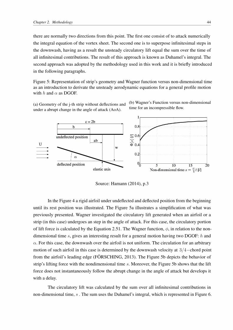
Chapter 2. Methodology 44
there are normally two directions from this point. The first one consist of to attack numericallythe integral equation of the vortex sheet. The second one is to superpose infinitesimal steps inthe downwash, having as a result the unsteady circulatory lift equal the sum over the time ofall infinitesimal contributions. The result of this approach is known as Duhamel’s integral. Thesecond approach was adopted by the methodology used in this work and it is briefly introducedin the following paragraphs.
Figure 5: Representation of strip’s geometry and Wagner function versus non-dimensional timeas an introduction to derivate the unsteady aerodynamic equations for a general profile motionwith h and α as DGOF.
(a) Geometry of the j-th strip without deflections andunder a abrupt change in the angle of attack (AoA).
(b) Wagner’s Function versus non-dimensionaltime for an incompressible flow.
Source: Hamann (2014), p.3
In the Figure 4 a rigid airfoil under undeflected and deflected position from the beginninguntil its rest position was illustrated. The Figure 5a illustrates a simplification of what waspreviously presented. Wagner investigated the circulatory lift generated when an airfoil or astrip (in this case) undergoes an step in the angle of attack. For this case, the circulatory portionof lift force is calculated by the Equation 2.51. The Wagner function, φ, in relation to the non-dimensional time s, gives an interesting result for a general motion having two DGOF: h andα. For this case, the downwash over the airfoil is not uniform. The circulation for an arbitrarymotion of such airfoil in this case is determined by the downwash velocity at 3/4−chord pointfrom the airfoil’s leading edge (FÖRSCHING, 2013). The Figure 5b depicts the behavior ofstrip’s lifting force with the nondimensional time s. Moreover, the Figure 5b shows that the liftforce does not instantaneously follow the abrupt change in the angle of attack but develops itwith a delay.
The circulatory lift was calculated by the sum over all infinitesimal contributions innon-dimensional time, s . The sum uses the Duhamel’s integral, which is represented in Figure 6.
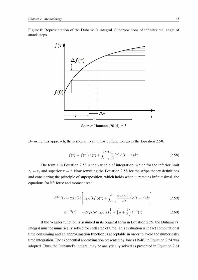
Chapter 2. Methodology 45
Figure 6: Representation of the Duhamel’s integral. Superpositions of infinitesimal angle ofattack steps.
Source: Hamann (2014), p.3
By using this approach, the response to an unit-step function gives the Equation 2.58.
f(t) = f(t0)A(t) +∫ τ=t
τ=t0
df
dt(τ)A(t− τ)dτ. (2.58)
The term τ in Equation 2.58 is the variable of integration, which for the inferior limitτ0 = t0 and superior τ = t. Now rewriting the Equation 2.58 for the strips theory definitionsand considering the principle of superposition, which holds when w remains infinitesimal, theequations for lift force and moment read:
`(C)(t) = 2πρUbw3/4(t0)φ(t) +
∫ t
τ=to
dw3/4(τ)dτ
φ(t− τ)dτ, (2.59)
m(C)(t) = −2πρUb2w3/4(t)12 +
(a+ 1
2
)`(C)(t). (2.60)
If the Wagner function is assumed in its original form in Equation 2.59, the Duhamel’sintegral must be numerically solved for each step of time. This evaluation is in fact computationaltime consuming and an approximation function is acceptable in order to avoid the numericallytime integration. The exponential approximation presented by Jones (1946) in Equation 2.54 wasadopted. Thus, the Duhamel’s integral may be analytically solved as presented in Equation 2.61
Chapter 2. Methodology 46
and Equation 2.62.
∫ τ=t
τ=to
dw 34(τ)
dτφ(t−τ)dτ = w 3
4(t)−w 3
4(t0)+
∫ t
to
dw 34(τ)
dτA1e
b1Ub
(t−τ)dτ+∫ t
to
dw 34(τ)
dτA2e
b2Ub
(t−τ)dτ
(2.61)
∫ τ=t
τ=to
dw 34(τ)
dτφ(t− τ)dτ = w 3
4(t)− w 3
4(t0) + λ1(t) + λ2(t). (2.62)
The terms λ1(t) and λ2(t) in Equation 2.62 are the lag state variables, introduced in theDuhamel’s integral to calculate the analytical solution. λ1(t) and λ2(t) can be defined by thedifferential equations in Equation 2.63 and Equation 2.64.
λ1(t) = a1U
bλ1(t) + A1w 3
4(t), (2.63)
λ2(t) = a2U
bλ2(t) + A2w 3
4(t). (2.64)
Considering a steady condition, the term w 34(t0) in Equation 2.62 is zero. So that, the
Equation 2.63 and Equation 2.64 can be inserted in Equation 2.62 resulting in the substitutionof numerical time integration by ordinary differential equations. That is the mean advantage toapproximate Wagner’s function by an exponential function (SILVESTRE, 2012). For this reason,the circulatory lift and pitching moment, are given in Equation 2.65 and Equation 2.66.
`(C)(t) = 2πρUb[w3/4(t) + λ1(t) + λ2(t)] (2.65)
m(C)(t) = −2πρUb2w3/4(t)12 +
(a+ 1
2
)`(C)(t) (2.66)
Regarding that the right term of the 2nd-order equation of motion ( see Equation 2.4)correspond to the generalized forces, which comprehend in the aerodynamic forces acting on theaircraft. The Equation 2.41 is the main equation to calculate de lift forces and has the first term(`(NC)) corresponding to the non circulatory lift and the second one `(C) to the circulatory lift.The non circulatory portion may be calculated by Equation 2.42 and the circulatory portion bythe Equation 2.65. These equations were used to calculate the unsteady aerodynamic behavior inlift forces and pitch moment calculations.
Furthermore, two equations are presented considering the fact that the deflection ofcontrol surfaces change the lift and pitching moment slope(SILVESTRE, 2012). The influenceof this surfaces connected at the wing’s trailing edge are represented by empirical equations infunction of the ratio of the control surface chord (cc) and strip chord (c): E = cc
c. The equation
for lift and moment coefficients with respect to a deflection of a flap (δc) are given by:
C`δc = C`α
π
[arccos(1− 2E) + 2
√E(1− E)
], (2.67)
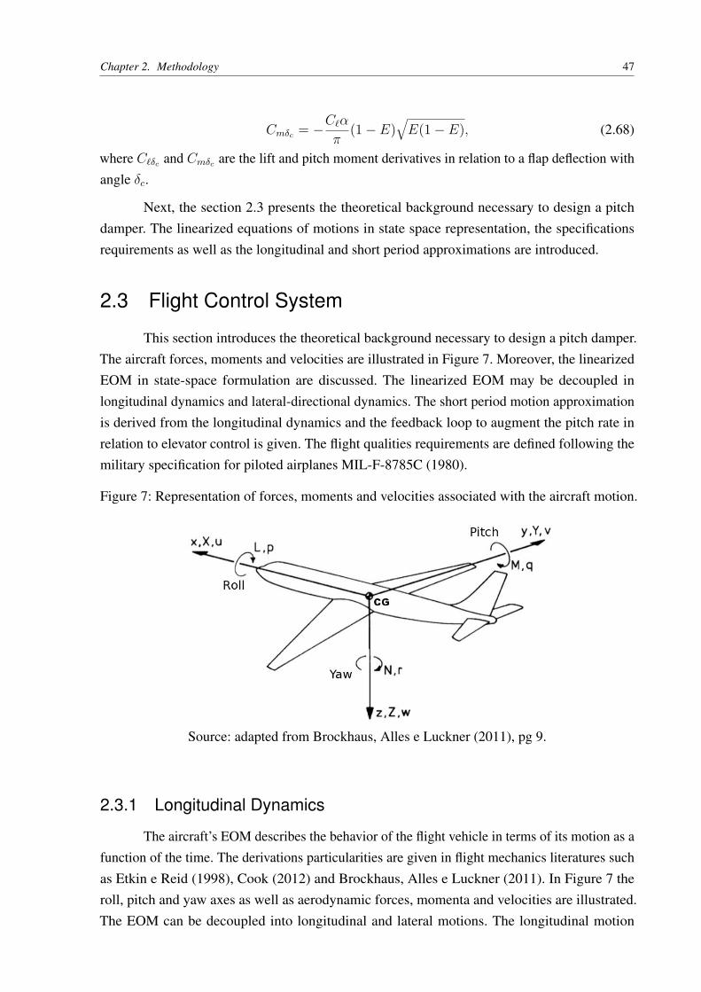
Chapter 2. Methodology 47
Cmδc = −C`απ
(1− E)√E(1− E), (2.68)
where C`δc and Cmδc are the lift and pitch moment derivatives in relation to a flap deflection withangle δc.
Next, the section 2.3 presents the theoretical background necessary to design a pitchdamper. The linearized equations of motions in state space representation, the specificationsrequirements as well as the longitudinal and short period approximations are introduced.
2.3 Flight Control System
This section introduces the theoretical background necessary to design a pitch damper.The aircraft forces, moments and velocities are illustrated in Figure 7. Moreover, the linearizedEOM in state-space formulation are discussed. The linearized EOM may be decoupled inlongitudinal dynamics and lateral-directional dynamics. The short period motion approximationis derived from the longitudinal dynamics and the feedback loop to augment the pitch rate inrelation to elevator control is given. The flight qualities requirements are defined following themilitary specification for piloted airplanes MIL-F-8785C (1980).
Figure 7: Representation of forces, moments and velocities associated with the aircraft motion.
Source: adapted from Brockhaus, Alles e Luckner (2011), pg 9.
2.3.1 Longitudinal Dynamics
The aircraft’s EOM describes the behavior of the flight vehicle in terms of its motion as afunction of the time. The derivations particularities are given in flight mechanics literatures suchas Etkin e Reid (1998), Cook (2012) and Brockhaus, Alles e Luckner (2011). In Figure 7 theroll, pitch and yaw axes as well as aerodynamic forces, momenta and velocities are illustrated.The EOM can be decoupled into longitudinal and lateral motions. The longitudinal motion
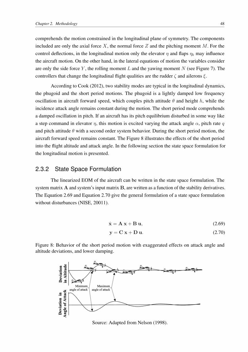
Chapter 2. Methodology 48
comprehends the motion constrained in the longitudinal plane of symmetry. The componentsincluded are only the axial force X , the normal force Z and the pitching moment M . For thecontrol deflections, in the longitudinal motion only the elevator η and flaps ηk may influencethe aircraft motion. On the other hand, in the lateral equations of motion the variables considerare only the side force Y , the rolling moment L and the yawing moment N (see Figure 7). Thecontrollers that change the longitudinal flight qualities are the rudder ζ and ailerons ξ.
According to Cook (2012), two stability modes are typical in the longitudinal dynamics,the phugoid and the short period motions. The phugoid is a lightly damped low frequencyoscillation in aircraft forward speed, which couples pitch attitude θ and height h, while theincidence attack angle remains constant during the motion. The short period mode comprehendsa damped oscillation in pitch. If an aircraft has its pitch equilibrium disturbed in some way likea step command in elevator η, this motion is excited varying the attack angle α, pitch rate qand pitch attitude θ with a second order system behavior. During the short period motion, theaircraft forward speed remains constant. The Figure 8 illustrates the effects of the short periodinto the flight altitude and attack angle. In the following section the state space formulation forthe longitudinal motion is presented.
2.3.2 State Space Formulation
The linearized EOM of the aircraft can be written in the state space formulation. Thesystem matrix A and system’s input matrix B, are written as a function of the stability derivatives.The Equation 2.69 and Equation 2.70 give the general formulation of a state space formulationwithout disturbances (NISE, 20011).
x = A x + B u, (2.69)
y = C x + D u. (2.70)
Figure 8: Behavior of the short period motion with exaggerated effects on attack angle andaltitude deviations, and lower damping.
Source: Adapted from Nelson (1998).
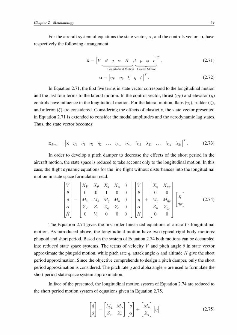
Chapter 2. Methodology 49
For the aircraft system of equations the state vector, x, and the controls vector, u, haverespectively the following arrangement:
x =[︸ ︷︷ ︸
Longitudinal Motion
V θ q α H ︸ ︷︷ ︸Lateral Motion
β p φ r]T, (2.71)
u =[ηF ηk ξ η ζ
]T. (2.72)
In Equation 2.71, the first five terms in state vector correspond to the longitudinal motionand the last four terms to the lateral motion. In the control vector, thrust (ηF ) and elevator (η)controls have influence in the longitudinal motion. For the lateral motion, flaps (ηk), rudder (ζ),and aileron (ξ) are considered. Considering the effects of elasticity, the state vector presentedin Equation 2.71 is extended to consider the modal amplitudes and the aerodynamic lag states.Thus, the state vector becomes:
xflex =[x η1 η1 η2 η2 . . . ηne ˙ηne λ11 λ21 . . . λ1j λ2j
]T. (2.73)
In order to develop a pitch damper to decrease the effects of the short period in theaircraft motion, the state space is reduced to take account only to the longitudinal motion. In thiscase, the flight dynamic equations for the line flight without disturbances into the longitudinalmotion in state space formulation read:
V
θ
q
α
H
=
XV Xθ Xq Xα 00 0 1 0 0MV Mθ Mq Mα 0ZV Zθ Zq Zα 00 V0 0 0 0
V
θ
q
α
H
+
Xη XηF
0 0Mη MηF
Zη ZηF0 0
ηηF
(2.74)
The Equation 2.74 gives the first order linearized equations of aircraft’s longitudinalmotion. As introduced above, the longitudinal motion have two typical rigid body motions:phugoid and short period. Based on the system of Equation 2.74 both motions can be decoupledinto reduced state space systems. The terms of velocity V and pitch angle θ in state vectorapproximate the phugoid motion, while pitch rate q, attack angle α and altitude H give the shortperiod approximation. Since the objective comprehends to design a pitch damper, only the shortperiod approximation is considered. The pitch rate q and alpha angle α are used to formulate theshort period state-space system approximation.
In face of the presented, the longitudinal motion system of Equation 2.74 are reduced tothe short period motion system of equations given in Equation 2.75.
qα
=Mq Mα
Zq Zα
qα
+Mη
Zη
[η] (2.75)
Chapter 2. Methodology 50
As written in Equation 2.75 the following characteristic equation can be written:
∆(s) = s2 − s(Mq + Zα) +MqZα −Mα = 0. (2.76)
According to Equation 2.76, the frequency and damping of the second order system arewritten in Equation 2.77 and Equation 2.78.
wSP ≈√ZαMq −Mα (2.77)
ζSP ≈12(Mq + Zα) (2.78)
2.3.3 Flying Qualities Requirements
The flying qualities requirements are stated in order to specify the performance criterianecessary to attend the safety and dynamic behavior of the aircraft. For this work the Amer-ican Military Specifications MIL-F-8785C (1980) is adopted. This document present severaldefinitions for aircraft’s lateral and longitudinal motions derived according to the aircraft class,flight phase category and level of flight qualities. One important fact is that the requirements aredeveloped based on the dynamics of classical aircraft whose short period is given by a secondorder function.
The flying qualities requirements are defined based on the aircraft flight phase, level offlight and flight envelope. The aircraft type can be classified in one of the following classes:
• Class I: small light airplanes;
• Class II: medium weight, low to medium maneuverability aircraft;
• Class III: Large, heavy, low to medium maneuverability aircraft;
• Class IV: High maneuverability aircraft;
The aircraft flight phase is defined based on the sequence of piloting tasks. The categoriesare:
• Category A: Non terminal flight phases that require rapid maneuvering, precision tracking,or precise flight path control.
• Category B: Non-terminal flight phases that require gradual maneuvering, less precisetracking and accurate flight path control.
• Category C: Terminal flight phases that require gradual maneuvering and precision flightpath control.
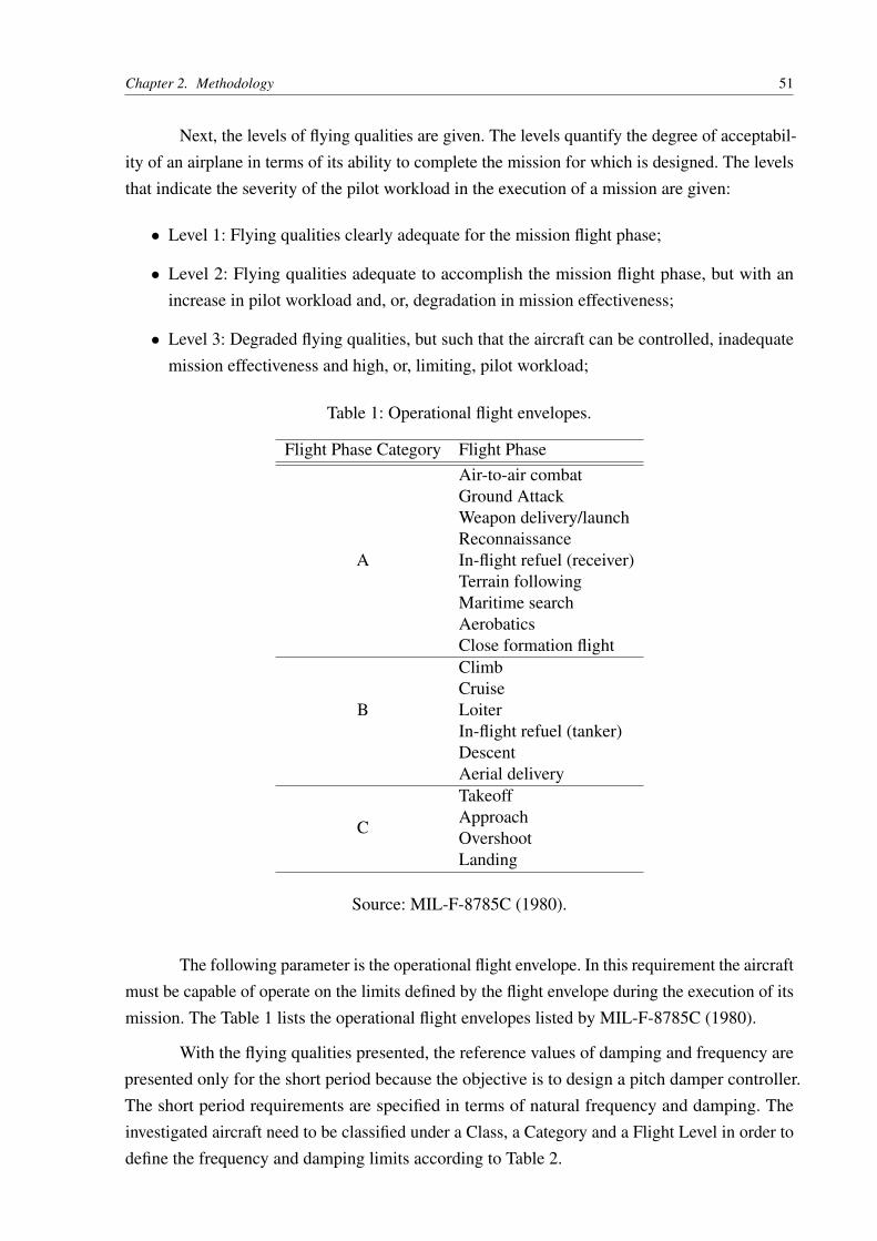
Chapter 2. Methodology 51
Next, the levels of flying qualities are given. The levels quantify the degree of acceptabil-ity of an airplane in terms of its ability to complete the mission for which is designed. The levelsthat indicate the severity of the pilot workload in the execution of a mission are given:
• Level 1: Flying qualities clearly adequate for the mission flight phase;
• Level 2: Flying qualities adequate to accomplish the mission flight phase, but with anincrease in pilot workload and, or, degradation in mission effectiveness;
• Level 3: Degraded flying qualities, but such that the aircraft can be controlled, inadequatemission effectiveness and high, or, limiting, pilot workload;
Table 1: Operational flight envelopes.
Flight Phase Category Flight Phase
A
Air-to-air combatGround AttackWeapon delivery/launchReconnaissanceIn-flight refuel (receiver)Terrain followingMaritime searchAerobaticsClose formation flight
B
ClimbCruiseLoiterIn-flight refuel (tanker)DescentAerial delivery
C
TakeoffApproachOvershootLanding
Source: MIL-F-8785C (1980).
The following parameter is the operational flight envelope. In this requirement the aircraftmust be capable of operate on the limits defined by the flight envelope during the execution of itsmission. The Table 1 lists the operational flight envelopes listed by MIL-F-8785C (1980).
With the flying qualities presented, the reference values of damping and frequency arepresented only for the short period because the objective is to design a pitch damper controller.The short period requirements are specified in terms of natural frequency and damping. Theinvestigated aircraft need to be classified under a Class, a Category and a Flight Level in order todefine the frequency and damping limits according to Table 2.
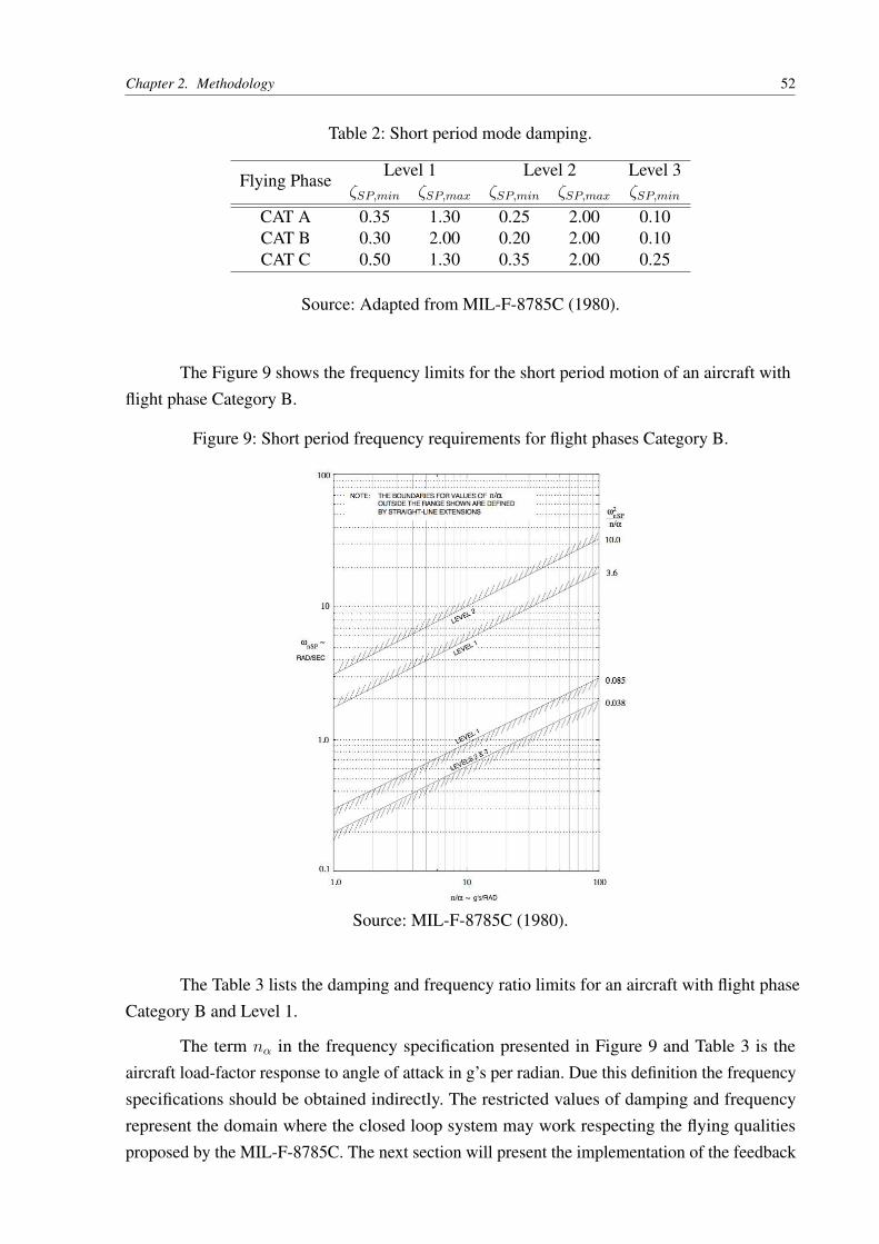
Chapter 2. Methodology 52
Table 2: Short period mode damping.
Flying PhaseLevel 1 Level 2 Level 3
ζSP,min ζSP,max ζSP,min ζSP,max ζSP,min
CAT A 0.35 1.30 0.25 2.00 0.10CAT B 0.30 2.00 0.20 2.00 0.10CAT C 0.50 1.30 0.35 2.00 0.25
Source: Adapted from MIL-F-8785C (1980).
The Figure 9 shows the frequency limits for the short period motion of an aircraft withflight phase Category B.
Figure 9: Short period frequency requirements for flight phases Category B.
Source: MIL-F-8785C (1980).
The Table 3 lists the damping and frequency ratio limits for an aircraft with flight phaseCategory B and Level 1.
The term nα in the frequency specification presented in Figure 9 and Table 3 is theaircraft load-factor response to angle of attack in g’s per radian. Due this definition the frequencyspecifications should be obtained indirectly. The restricted values of damping and frequencyrepresent the domain where the closed loop system may work respecting the flying qualitiesproposed by the MIL-F-8785C. The next section will present the implementation of the feedback
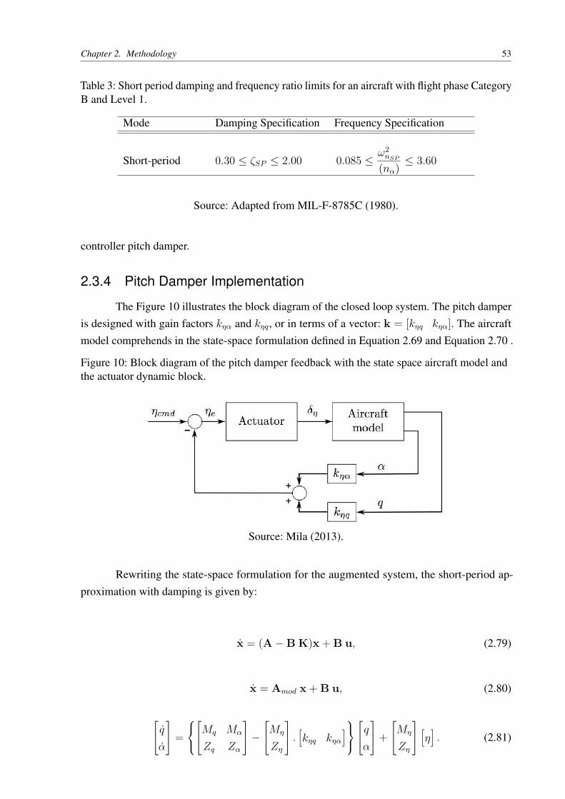
Chapter 2. Methodology 53
Table 3: Short period damping and frequency ratio limits for an aircraft with flight phase CategoryB and Level 1.
Mode Damping Specification Frequency Specification
Short-period 0.30 ≤ ζSP ≤ 2.00 0.085 ≤ω2nSP
(nα) ≤ 3.60
Source: Adapted from MIL-F-8785C (1980).
controller pitch damper.
2.3.4 Pitch Damper Implementation
The Figure 10 illustrates the block diagram of the closed loop system. The pitch damperis designed with gain factors kηα and kηq, or in terms of a vector: k = [kηq kηα]. The aircraftmodel comprehends in the state-space formulation defined in Equation 2.69 and Equation 2.70 .
Figure 10: Block diagram of the pitch damper feedback with the state space aircraft model andthe actuator dynamic block.
Source: Mila (2013).
Rewriting the state-space formulation for the augmented system, the short-period ap-proximation with damping is given by:
x = (A−B K)x + B u, (2.79)
x = Amod x + B u, (2.80)
qα
=
Mq Mα
Zq Zα
−Mη
Zη
. [kηq kηα]qα
+Mη
Zη
[η] . (2.81)
Chapter 2. Methodology 54
The characteristic equation of the modified system is given in Equation 2.82.
∆(s) = |sI−Amod| = |sI + A + B k| = 0 (2.82)
In the Equation 2.82 the the system’s closed loop frequency ω∗nSP and damping ζ∗SP maybe calculated, respectively, by respecting the following equations:
ω∗nSP =√
(Mq −Mηkηq).(Zα − Zηkηα)− (Mα −Mηkηα)(Zq − Zηkηq), (2.83)
ζ∗SP = Mηkηq − Zα −Mα + Zηkηα2ωnsp
(2.84)
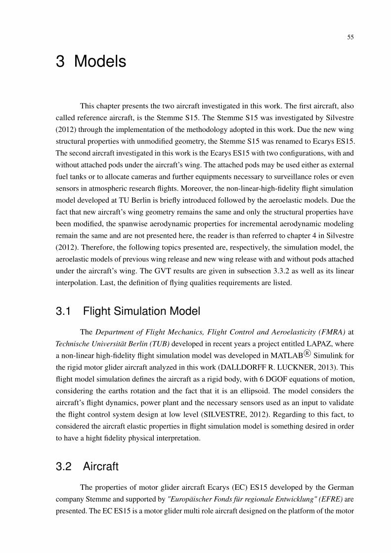
55
3 Models
This chapter presents the two aircraft investigated in this work. The first aircraft, alsocalled reference aircraft, is the Stemme S15. The Stemme S15 was investigated by Silvestre(2012) through the implementation of the methodology adopted in this work. Due the new wingstructural properties with unmodified geometry, the Stemme S15 was renamed to Ecarys ES15.The second aircraft investigated in this work is the Ecarys ES15 with two configurations, with andwithout attached pods under the aircraft’s wing. The attached pods may be used either as externalfuel tanks or to allocate cameras and further equipments necessary to surveillance roles or evensensors in atmospheric research flights. Moreover, the non-linear-high-fidelity flight simulationmodel developed at TU Berlin is briefly introduced followed by the aeroelastic models. Due thefact that new aircraft’s wing geometry remains the same and only the structural properties havebeen modified, the spanwise aerodynamic properties for incremental aerodynamic modelingremain the same and are not presented here, the reader is than referred to chapter 4 in Silvestre(2012). Therefore, the following topics presented are, respectively, the simulation model, theaeroelastic models of previous wing release and new wing release with and without pods attachedunder the aircraft’s wing. The GVT results are given in subsection 3.3.2 as well as its linearinterpolation. Last, the definition of flying qualities requirements are listed.
3.1 Flight Simulation Model
The Department of Flight Mechanics, Flight Control and Aeroelasticity (FMRA) atTechnische Universität Berlin (TUB) developed in recent years a project entitled LAPAZ, wherea non-linear high-fidelity flight simulation model was developed in MATLAB R© Simulink forthe rigid motor glider aircraft analyzed in this work (DALLDORFF R. LUCKNER, 2013). Thisflight model simulation defines the aircraft as a rigid body, with 6 DGOF equations of motion,considering the earths rotation and the fact that it is an ellipsoid. The model considers theaircraft’s flight dynamics, power plant and the necessary sensors used as an input to validatethe flight control system design at low level (SILVESTRE, 2012). Regarding to this fact, toconsidered the aircraft elastic properties in flight simulation model is something desired in orderto have a hight fidelity physical interpretation.
3.2 Aircraft
The properties of motor glider aircraft Ecarys (EC) ES15 developed by the Germancompany Stemme and supported by "Europäischer Fonds für regionale Entwicklung" (EFRE) arepresented. The EC ES15 is a motor glider multi role aircraft designed on the platform of the motor
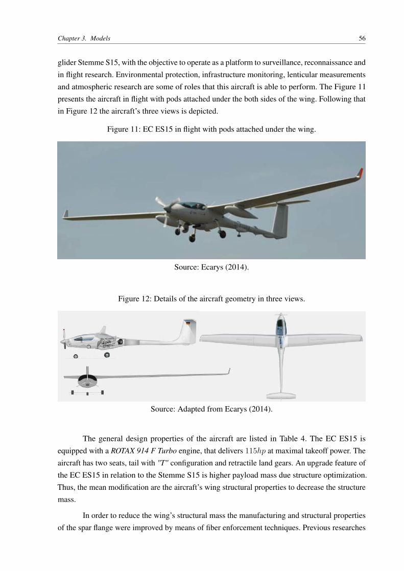
Chapter 3. Models 56
glider Stemme S15, with the objective to operate as a platform to surveillance, reconnaissance andin flight research. Environmental protection, infrastructure monitoring, lenticular measurementsand atmospheric research are some of roles that this aircraft is able to perform. The Figure 11presents the aircraft in flight with pods attached under the both sides of the wing. Following thatin Figure 12 the aircraft’s three views is depicted.
Figure 11: EC ES15 in flight with pods attached under the wing.
Source: Ecarys (2014).
Figure 12: Details of the aircraft geometry in three views.
Source: Adapted from Ecarys (2014).
The general design properties of the aircraft are listed in Table 4. The EC ES15 isequipped with a ROTAX 914 F Turbo engine, that delivers 115hp at maximal takeoff power. Theaircraft has two seats, tail with "T" configuration and retractile land gears. An upgrade feature ofthe EC ES15 in relation to the Stemme S15 is higher payload mass due structure optimization.Thus, the mean modification are the aircraft’s wing structural properties to decrease the structuremass.
In order to reduce the wing’s structural mass the manufacturing and structural propertiesof the spar flange were improved by means of fiber enforcement techniques. Previous researches
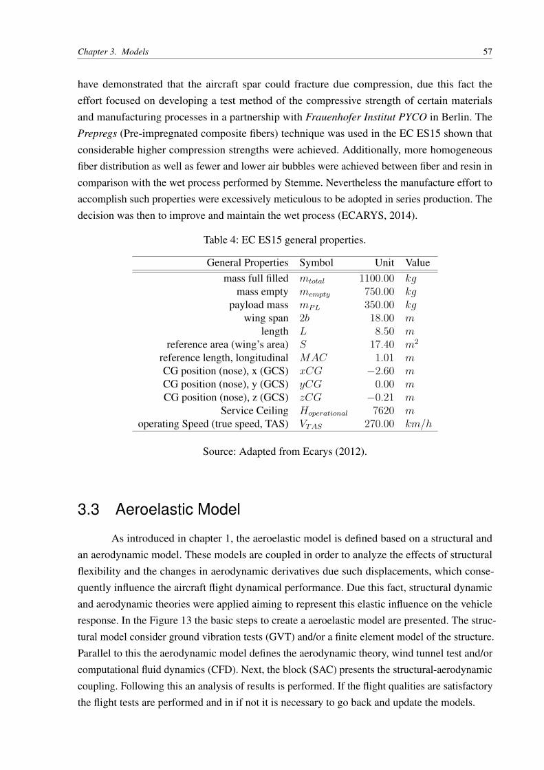
Chapter 3. Models 57
have demonstrated that the aircraft spar could fracture due compression, due this fact theeffort focused on developing a test method of the compressive strength of certain materialsand manufacturing processes in a partnership with Frauenhofer Institut PYCO in Berlin. ThePrepregs (Pre-impregnated composite fibers) technique was used in the EC ES15 shown thatconsiderable higher compression strengths were achieved. Additionally, more homogeneousfiber distribution as well as fewer and lower air bubbles were achieved between fiber and resin incomparison with the wet process performed by Stemme. Nevertheless the manufacture effort toaccomplish such properties were excessively meticulous to be adopted in series production. Thedecision was then to improve and maintain the wet process (ECARYS, 2014).
Table 4: EC ES15 general properties.
General Properties Symbol Unit Valuemass full filled mtotal 1100.00 kg
mass empty mempty 750.00 kgpayload mass mPL 350.00 kg
wing span 2b 18.00 mlength L 8.50 m
reference area (wing’s area) S 17.40 m2
reference length, longitudinal MAC 1.01 mCG position (nose), x (GCS) xCG −2.60 mCG position (nose), y (GCS) yCG 0.00 mCG position (nose), z (GCS) zCG −0.21 m
Service Ceiling Hoperational 7620 moperating Speed (true speed, TAS) VTAS 270.00 km/h
Source: Adapted from Ecarys (2012).
3.3 Aeroelastic Model
As introduced in chapter 1, the aeroelastic model is defined based on a structural andan aerodynamic model. These models are coupled in order to analyze the effects of structuralflexibility and the changes in aerodynamic derivatives due such displacements, which conse-quently influence the aircraft flight dynamical performance. Due this fact, structural dynamicand aerodynamic theories were applied aiming to represent this elastic influence on the vehicleresponse. In the Figure 13 the basic steps to create a aeroelastic model are presented. The struc-tural model consider ground vibration tests (GVT) and/or a finite element model of the structure.Parallel to this the aerodynamic model defines the aerodynamic theory, wind tunnel test and/orcomputational fluid dynamics (CFD). Next, the block (SAC) presents the structural-aerodynamiccoupling. Following this an analysis of results is performed. If the flight qualities are satisfactorythe flight tests are performed and in if not it is necessary to go back and update the models.
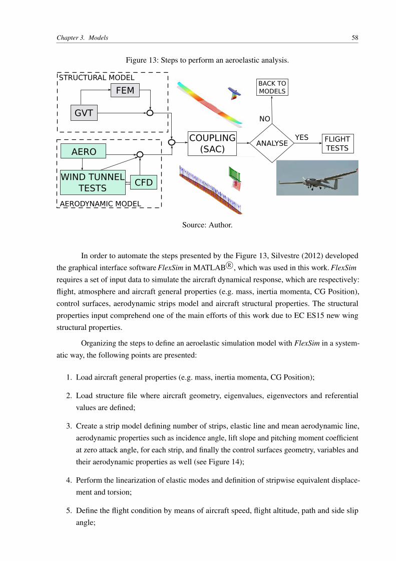
Chapter 3. Models 58
Figure 13: Steps to perform an aeroelastic analysis.
GVT
FEM
AERO
COUPLING(SAC)
AERODYNAMIC MODEL
STRUCTURAL MODEL
ANALYSEYES
NO
FLIGHT TESTS
BACK TOMODELS
WIND TUNNELTESTS
CFD
Source: Author.
In order to automate the steps presented by the Figure 13, Silvestre (2012) developedthe graphical interface software FlexSim in MATLAB R©, which was used in this work. FlexSim
requires a set of input data to simulate the aircraft dynamical response, which are respectively:flight, atmosphere and aircraft general properties (e.g. mass, inertia momenta, CG Position),control surfaces, aerodynamic strips model and aircraft structural properties. The structuralproperties input comprehend one of the main efforts of this work due to EC ES15 new wingstructural properties.
Organizing the steps to define an aeroelastic simulation model with FlexSim in a system-atic way, the following points are presented:
1. Load aircraft general properties (e.g. mass, inertia momenta, CG Position);
2. Load structure file where aircraft geometry, eigenvalues, eigenvectors and referentialvalues are defined;
3. Create a strip model defining number of strips, elastic line and mean aerodynamic line,aerodynamic properties such as incidence angle, lift slope and pitching moment coefficientat zero attack angle, for each strip, and finally the control surfaces geometry, variables andtheir aerodynamic properties as well (see Figure 14);
4. Perform the linearization of elastic modes and definition of stripwise equivalent displace-ment and torsion;
5. Define the flight condition by means of aircraft speed, flight altitude, path and side slipangle;
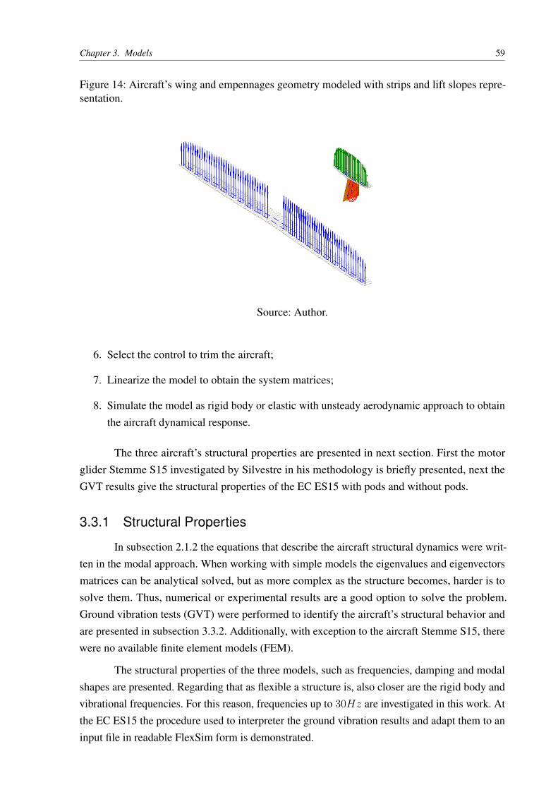
Chapter 3. Models 59
Figure 14: Aircraft’s wing and empennages geometry modeled with strips and lift slopes repre-sentation.
Source: Author.
6. Select the control to trim the aircraft;
7. Linearize the model to obtain the system matrices;
8. Simulate the model as rigid body or elastic with unsteady aerodynamic approach to obtainthe aircraft dynamical response.
The three aircraft’s structural properties are presented in next section. First the motorglider Stemme S15 investigated by Silvestre in his methodology is briefly presented, next theGVT results give the structural properties of the EC ES15 with pods and without pods.
3.3.1 Structural Properties
In subsection 2.1.2 the equations that describe the aircraft structural dynamics were writ-ten in the modal approach. When working with simple models the eigenvalues and eigenvectorsmatrices can be analytical solved, but as more complex as the structure becomes, harder is tosolve them. Thus, numerical or experimental results are a good option to solve the problem.Ground vibration tests (GVT) were performed to identify the aircraft’s structural behavior andare presented in subsection 3.3.2. Additionally, with exception to the aircraft Stemme S15, therewere no available finite element models (FEM).
The structural properties of the three models, such as frequencies, damping and modalshapes are presented. Regarding that as flexible a structure is, also closer are the rigid body andvibrational frequencies. For this reason, frequencies up to 30Hz are investigated in this work. Atthe EC ES15 the procedure used to interpreter the ground vibration results and adapt them to aninput file in readable FlexSim form is demonstrated.
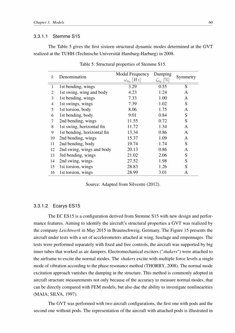
Chapter 3. Models 60
3.3.1.1 Stemme S15
The Table 5 gives the first sixteen structural dynamic modes determined at the GVTrealized at the TUHH (Technische Universität Hamburg-Harburg) in 2008.
Table 5: Structural properties of Stemme S15.
k DenominationModal Frequency Damping
Symmetryωnk [Hz] ζnk [%]
1 1st bending, wings 3.29 0.55 S2 1st swing, wing and body 4.23 1.24 A3 1st bending, wings 7.33 1.00 A4 1st swings, wings 7.39 1.02 S5 1st torsion, body 8.06 1.75 A6 1st bending, body 9.01 0.84 S7 2nd bending, wings 11.55 0.72 S8 1st swing, horizontal fin 11.72 1.34 A9 1st bending, horizontal fin 13.34 0.86 A10 2nd bending, wings 15.37 1.09 A11 2nd bending, body 19.74 1.74 S12 2nd swing, wings and body 20.13 0.86 A13 3rd bending, wings 21.02 2.06 S14 2nd swing, wings 27.52 1.98 S15 1st torsion, wings 28.83 1.26 S16 1st torsion, wings 28.99 3.01 A
Source: Adapted from Silvestre (2012).
3.3.1.2 Ecarys ES15
The EC ES15 is a configuration derived from Stemme S15 with new design and perfor-mance features. Aiming to identify the aircraft’s structural properties a GVT was realized bythe company Leichtwerk in May 2015 in Braunschweig, Germany. The Figure 15 presents theaircraft under tests with a set of accelerometers attached at wing, fuselage and empennages. Thetests were performed separately with fixed and free controls, the aircraft was supported by biginner tubes that worked as air dampers. Electromechanical exciters ("shakers") were attached tothe airframe to excite the normal modes. The shakers excite with multiple force levels a singlemode of vibration according to the phase resonance method (THORBY, 2008). The normal modeexcitation approach vanishes the damping in the structure. This method is commonly adopted inaircraft structure measurements not only because of the accuracy to measure normal modes, thatcan be directly compared with FEM models, but also due the ability to investigate nonlinearities(MAIA; SILVA, 1997).
The GVT was performed with two aircraft configurations, the first one with pods and thesecond one without pods. The representation of the aircraft with attached pods is illustrated in
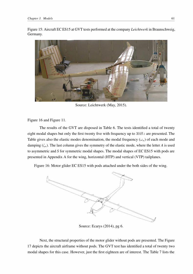
Chapter 3. Models 61
Figure 15: Aircraft EC ES15 at GVT tests performed at the company Leichtwerk in Braunschweig,Germany.
Source: Leichtwerk (May, 2015).
Figure 16 and Figure 11.
The results of the GVT are disposed in Table 6. The tests identified a total of twentyeight modal shapes but only the first twenty five with frequency up to 30Hz are presented. TheTable gives also the elastic modes denomination, the modal frequency (ωn) of each mode anddamping (ζn). The last column gives the symmetry of the elastic mode, where the letter A is usedto asymmetric and S for symmetric modal shapes. The modal shapes of EC ES15 with pods arepresented in Appendix A for the wing, horizontal (HTP) and vertical (VTP) tailplanes.
Figure 16: Motor glider EC ES15 with pods attached under the both sides of the wing.
Source: Ecarys (2014), pg 6.
Next, the structural properties of the motor glider without pods are presented. The Figure17 depicts the aircraft airframe without pods. The GVT test has identified a total of twenty twomodal shapes for this case. However, just the first eighteen are of interest. The Table 7 lists the
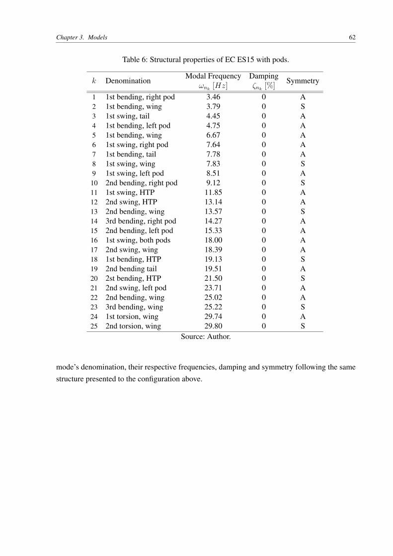
Chapter 3. Models 62
Table 6: Structural properties of EC ES15 with pods.
k DenominationModal Frequency Damping
Symmetryωnk [Hz] ζnk [%]
1 1st bending, right pod 3.46 0 A2 1st bending, wing 3.79 0 S3 1st swing, tail 4.45 0 A4 1st bending, left pod 4.75 0 A5 1st bending, wing 6.67 0 A6 1st swing, right pod 7.64 0 A7 1st bending, tail 7.78 0 A8 1st swing, wing 7.83 0 S9 1st swing, left pod 8.51 0 A10 2nd bending, right pod 9.12 0 S11 1st swing, HTP 11.85 0 A12 2nd swing, HTP 13.14 0 A13 2nd bending, wing 13.57 0 S14 3rd bending, right pod 14.27 0 A15 2nd bending, left pod 15.33 0 A16 1st swing, both pods 18.00 0 A17 2nd swing, wing 18.39 0 A18 1st bending, HTP 19.13 0 S19 2nd bending tail 19.51 0 A20 2st bending, HTP 21.50 0 S21 2nd swing, left pod 23.71 0 A22 2nd bending, wing 25.02 0 A23 3rd bending, wing 25.22 0 S24 1st torsion, wing 29.74 0 A25 2nd torsion, wing 29.80 0 S
Source: Author.
mode’s denomination, their respective frequencies, damping and symmetry following the samestructure presented to the configuration above.
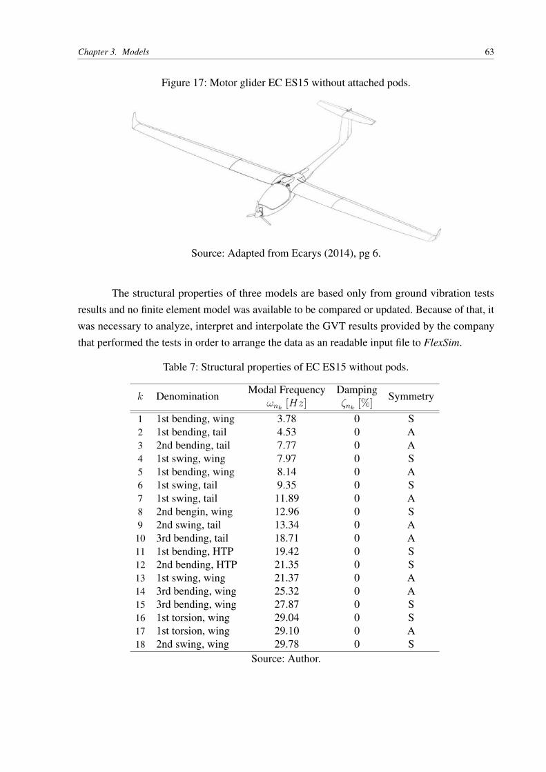
Chapter 3. Models 63
Figure 17: Motor glider EC ES15 without attached pods.
Source: Adapted from Ecarys (2014), pg 6.
The structural properties of three models are based only from ground vibration testsresults and no finite element model was available to be compared or updated. Because of that, itwas necessary to analyze, interpret and interpolate the GVT results provided by the companythat performed the tests in order to arrange the data as an readable input file to FlexSim.
Table 7: Structural properties of EC ES15 without pods.
k DenominationModal Frequency Damping
Symmetryωnk [Hz] ζnk [%]
1 1st bending, wing 3.78 0 S2 1st bending, tail 4.53 0 A3 2nd bending, tail 7.77 0 A4 1st swing, wing 7.97 0 S5 1st bending, wing 8.14 0 A6 1st swing, tail 9.35 0 S7 1st swing, tail 11.89 0 A8 2nd bengin, wing 12.96 0 S9 2nd swing, tail 13.34 0 A10 3rd bending, tail 18.71 0 A11 1st bending, HTP 19.42 0 S12 2nd bending, HTP 21.35 0 S13 1st swing, wing 21.37 0 A14 3rd bending, wing 25.32 0 A15 3rd bending, wing 27.87 0 S16 1st torsion, wing 29.04 0 S17 1st torsion, wing 29.10 0 A18 2nd swing, wing 29.78 0 S
Source: Author.
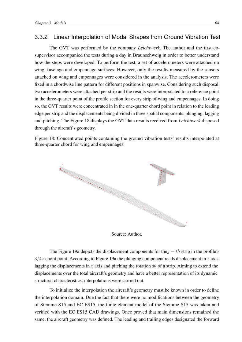
Chapter 3. Models 64
3.3.2 Linear Interpolation of Modal Shapes from Ground Vibration Test
The GVT was performed by the company Leichtwerk. The author and the first co-supervisor accompanied the tests during a day in Braunschweig in order to better understandhow the steps were developed. To perform the test, a set of accelerometers were attached onwing, fuselage and empennage surfaces. However, only the results measured by the sensorsattached on wing and empennages were considered in the analysis. The accelerometers werefixed in a chordwise line pattern for different positions in spanwise. Considering such disposal,two accelerometers were attached per strip and the results were interpolated to a reference pointin the three-quarter point of the profile section for every strip of wing and empennages. In doingso, the GVT results were concentrated in in the one-quarter chord point in relation to the leadingedge per strip and the displacements being divided in three spatial components: plunging, laggingand pitching. The Figure 18 displays the GVT data results received from Leichtwerk disposedthrough the aircraft’s geometry.
Figure 18: Concentrated points containing the ground vibration tests’ results interpolated atthree-quarter chord for wing and empennages.
Source: Author.
The Figure 19a depicts the displacement components for thej − th strip in the profile’s3/4×chord point. According to Figure 19a the plunging component reads displacement in z axis,lagging the displacements in x axis and pitching the rotation dθ of a strip. Aiming to extend thedisplacements over the total aircraft’s geometry and have a better representation of its dynamicstructural characteristics, interpolations were carried out.
To initialize the interpolation the aircraft’s geometry must be known in order to definethe interpolation domain. Due the fact that there were no modifications between the geometryof Stemme S15 and EC ES15, the finite element model of the Stemme S15 was taken andverified with the EC ES15 CAD drawings. Once proved that main dimensions remained thesame, the aircraft geometry was defined. The leading and trailing edges designated the forward
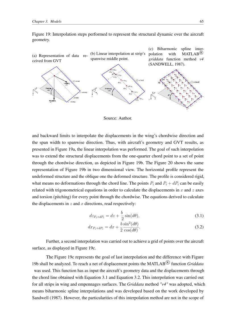
Chapter 3. Models 65
Figure 19: Interpolation steps performed to represent the structural dynamic over the aircraftgeometry.
(a) Representation of data re-ceived from GVT
(b) Linear interpolation at strip’sspanwise middle point.
(c) Biharmonic spline inter-polation with MATLAB R©griddata function method v4(SANDWELL, 1987).
Source: Author.
and backward limits to interpolate the displacements in the wing’s chordwise direction andthe span width to spanwise direction. Thus, with aircraft’s geometry and GVT results, aspresented in Figure 19a, the linear interpolation was performed. The goal of such interpolationwas to extend the structural displacements from the one-quarter chord point to a set of pointthrough the chordwise direction, as depicted in Figure 19b. The Figure 20 shows the samerepresentation of Figure 19b in two dimensional view. The horizontal profile represent theundeformed structure and the oblique one the deformed structure. The profile is considered rigid,what means no deformations through the chord line. The points Pi and Pi + dPi can be easilyrelated with trigonometrical equations in order to calculate the displacements in x and z axesand torsion (pitching) for every point through the chordwise. The equations derived to calculatethe displacements in z and x directions, read respectively:
dzPi+dPi = dz + b
2 sin(dθ), (3.1)
dxPi+dPi = dx+ b
2sin2(dθ)cos(dθ) . (3.2)
Further, a second interpolation was carried out to achieve a grid of points over the aircraftsurface, as displayed in Figure 19c.
The Figure 19c represents the goal of last interpolation and the difference with Figure19b shall be analyzed. To reach a net of displacement points the MATLAB R© function Griddata
was used. This function has as input the aircraft’s geometry data and the displacements throughthe chord line obtained with Equation 3.1 and Equation 3.2. This interpolation was carried outfor all strips in wing and empennages surfaces. The Griddata method "v4" was adopted, whichmeans biharmonic spline interpolations and was developed based on the work developed bySandwell (1987). However, the particularities of this interpolation method are not in the scope of
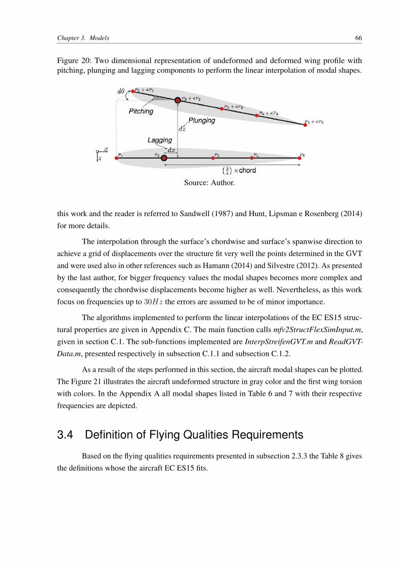
Chapter 3. Models 66
Figure 20: Two dimensional representation of undeformed and deformed wing profile withpitching, plunging and lagging components to perform the linear interpolation of modal shapes.
Source: Author.
this work and the reader is referred to Sandwell (1987) and Hunt, Lipsman e Rosenberg (2014)for more details.
The interpolation through the surface’s chordwise and surface’s spanwise direction toachieve a grid of displacements over the structure fit very well the points determined in the GVTand were used also in other references such as Hamann (2014) and Silvestre (2012). As presentedby the last author, for bigger frequency values the modal shapes becomes more complex andconsequently the chordwise displacements become higher as well. Nevertheless, as this workfocus on frequencies up to 30Hz the errors are assumed to be of minor importance.
The algorithms implemented to perform the linear interpolations of the EC ES15 struc-tural properties are given in Appendix C. The main function calls mfv2StructFlexSimInput.m,given in section C.1. The sub-functions implemented are InterpStreifenGVT.m and ReadGVT-
Data.m, presented respectively in subsection C.1.1 and subsection C.1.2.
As a result of the steps performed in this section, the aircraft modal shapes can be plotted.The Figure 21 illustrates the aircraft undeformed structure in gray color and the first wing torsionwith colors. In the Appendix A all modal shapes listed in Table 6 and 7 with their respectivefrequencies are depicted.
3.4 Definition of Flying Qualities Requirements
Based on the flying qualities requirements presented in subsection 2.3.3 the Table 8 givesthe definitions whose the aircraft EC ES15 fits.
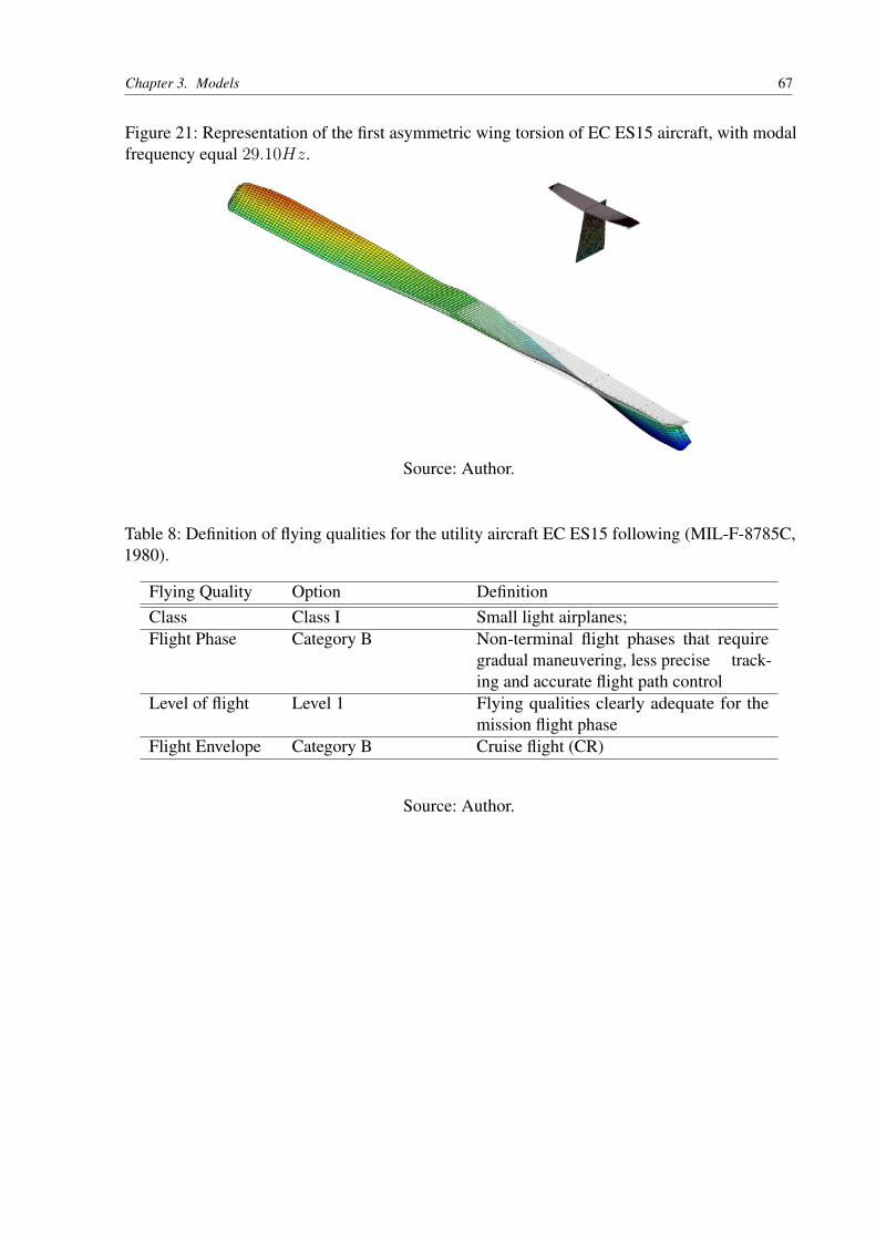
Chapter 3. Models 67
Figure 21: Representation of the first asymmetric wing torsion of EC ES15 aircraft, with modalfrequency equal 29.10Hz.
Source: Author.
Table 8: Definition of flying qualities for the utility aircraft EC ES15 following (MIL-F-8785C,1980).
Flying Quality Option DefinitionClass Class I Small light airplanes;Flight Phase Category B Non-terminal flight phases that require
gradual maneuvering, less precise track-ing and accurate flight path control
Level of flight Level 1 Flying qualities clearly adequate for themission flight phase
Flight Envelope Category B Cruise flight (CR)
Source: Author.
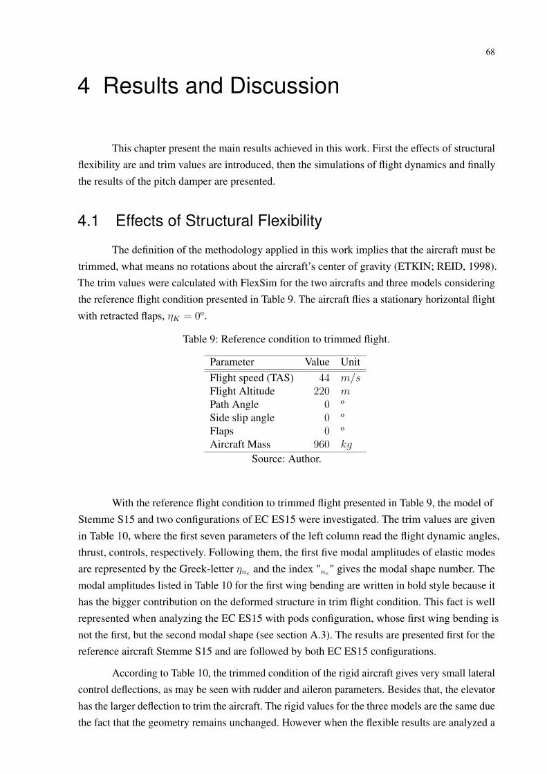
68
4 Results and Discussion
This chapter present the main results achieved in this work. First the effects of structuralflexibility are and trim values are introduced, then the simulations of flight dynamics and finallythe results of the pitch damper are presented.
4.1 Effects of Structural Flexibility
The definition of the methodology applied in this work implies that the aircraft must betrimmed, what means no rotations about the aircraft’s center of gravity (ETKIN; REID, 1998).The trim values were calculated with FlexSim for the two aircrafts and three models consideringthe reference flight condition presented in Table 9. The aircraft flies a stationary horizontal flightwith retracted flaps, ηK = 0o.
Table 9: Reference condition to trimmed flight.
Parameter Value UnitFlight speed (TAS) 44 m/sFlight Altitude 220 mPath Angle 0 o
Side slip angle 0 o
Flaps 0 o
Aircraft Mass 960 kg
Source: Author.
With the reference flight condition to trimmed flight presented in Table 9, the model ofStemme S15 and two configurations of EC ES15 were investigated. The trim values are givenin Table 10, where the first seven parameters of the left column read the flight dynamic angles,thrust, controls, respectively. Following them, the first five modal amplitudes of elastic modesare represented by the Greek-letter ηne and the index "ne" gives the modal shape number. Themodal amplitudes listed in Table 10 for the first wing bending are written in bold style because ithas the bigger contribution on the deformed structure in trim flight condition. This fact is wellrepresented when analyzing the EC ES15 with pods configuration, whose first wing bending isnot the first, but the second modal shape (see section A.3). The results are presented first for thereference aircraft Stemme S15 and are followed by both EC ES15 configurations.
According to Table 10, the trimmed condition of the rigid aircraft gives very small lateralcontrol deflections, as may be seen with rudder and aileron parameters. Besides that, the elevatorhas the larger deflection to trim the aircraft. The rigid values for the three models are the same duethe fact that the geometry remains unchanged. However when the flexible results are analyzed a
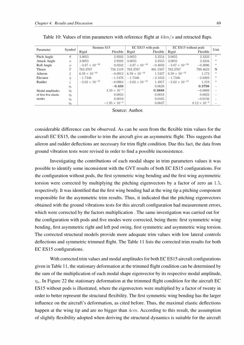
Chapter 4. Results and Discussion 69
Table 10: Values of trim parameters with reference flight at 44m/s and retracted flaps.
Parameter SymbolStemme S15 EC ES15 with pods EC ES15 without pods
UnitRigid Flexible Rigid Flexible Rigid Flexible
Pitch Angle θ 3.0055 2.9502 3.0055 3.3554 3.0055 3.3233 o
Attack Angle α 3.0055 2.9502 3.0055 3.3555 3.0055 3.3234 o
Roll Angle φ −3.87× 10⁻¹⁸ 0.0242 −3.87× 10⁻¹⁸ −0.4033 −3.87× 10⁻¹⁸ −0.3096 o
Thrust T 763.3767 758.1519 763.3767 801.5507 763.3767 799.4623 NAileron ξ 6.59× 10⁻¹² −0.0912 6.59× 10⁻¹² 1.5327 6.59× 10⁻¹² 1.173 o
Elevator η −1.7346 −1.5476 −1.7346 −2.1832 −1.7346 −2.0203 o
Rudder ζ −2.62× 10⁻¹⁵ −0.0964 −2.62× 10⁻¹⁵ 1.4917 −2.62× 10⁻¹⁵ 1.219 o
Modal amplitudesof first five elasticmodes
η1 −0.459 0.0628 0.3798 -η2 4.33× 10⁻⁴ 0.3888 −0.0069 -η3 0.0024 0.0018 0.0022 -η4 0.0019 0.0165 −0.0156 -η5 −1.95× 10⁻⁴ 0.0047 8.12× 10⁻⁴ -
Source: Author.
considerable difference can be observed. As can be seen from the flexible trim values for theaircraft EC ES15, the controller to trim the aircraft give an asymmetric flight. This suggests thataileron and rudder deflections are necessary for trim flight condition. Due this fact, the data fromground vibration tests were revised in order to find a possible inconsistence.
Investigating the contributions of each modal shape in trim parameters values it waspossible to identify some inconsistent with the GVT results of both EC ES15 configurations. Forthe configuration without pods, the first symmetric wing bending and the first wing asymmetrictorsion were corrected by multiplying the pitching eigenvectors by a factor of zero an 1.5,respectively. It was identified that the first wing bending had at the wing tip a pitching componentresponsible for the asymmetric trim results. Thus, it indicated that the pitching eigenvectorsobtained with the ground vibrations tests for this aircraft configuration had measurement errors,which were corrected by the factors multiplication . The same investigation was carried out forthe configuration with pods and five modes were corrected, being them: first symmetric wingbending, first asymmetric right and left pod swing, first symmetric and asymmetric wing torsion.The corrected structural models provide more adequate trim values with low lateral controlsdeflections and symmetric trimmed flight. The Table 11 lists the corrected trim results for bothEC ES15 configurations.
With corrected trim values and modal amplitudes for both EC ES15 aircraft configurationsgiven in Table 11, the stationary deformation at the trimmed flight condition can be determined bythe sum of the multiplication of each modal shape eigenvector by its respective modal amplitude,ηn. In Figure 22 the stationary deformation at the trimmed flight condition for the aircraft ECES15 without pods is illustrated, where the eigenvectors were multiplied by a factor of twenty inorder to better represent the structural flexibility. The first symmetric wing bending has the largerinfluence on the aircraft’s deformation, as cited before. Thus, the maximal elastic deflectionshappen at the wing tip and are no bigger than 4cm. According to this result, the assumptionof slightly flexibility adopted when deriving the structural dynamics is suitable for the aircraft
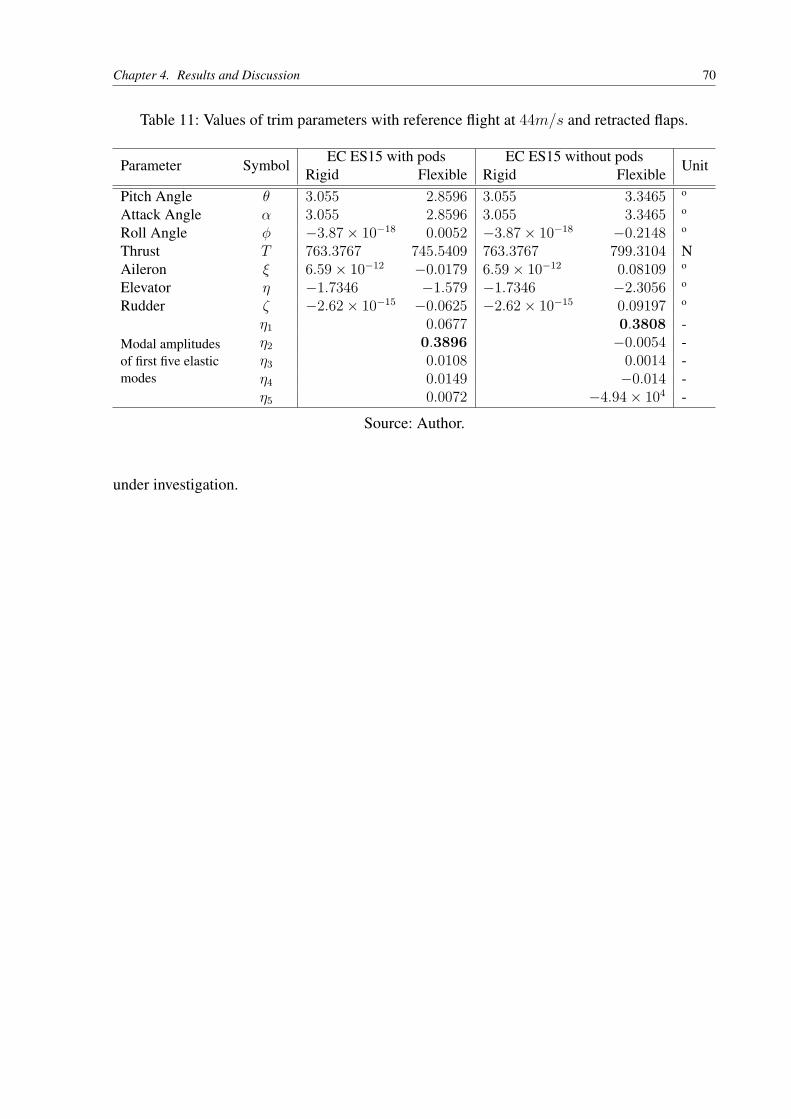
Chapter 4. Results and Discussion 70
Table 11: Values of trim parameters with reference flight at 44m/s and retracted flaps.
Parameter SymbolEC ES15 with pods EC ES15 without pods
UnitRigid Flexible Rigid Flexible
Pitch Angle θ 3.055 2.8596 3.055 3.3465 o
Attack Angle α 3.055 2.8596 3.055 3.3465 o
Roll Angle φ −3.87× 10⁻¹⁸ 0.0052 −3.87× 10⁻¹⁸ −0.2148 o
Thrust T 763.3767 745.5409 763.3767 799.3104 NAileron ξ 6.59× 10⁻¹² −0.0179 6.59× 10⁻¹² 0.08109 o
Elevator η −1.7346 −1.579 −1.7346 −2.3056 o
Rudder ζ −2.62× 10⁻¹⁵ −0.0625 −2.62× 10⁻¹⁵ 0.09197 o
Modal amplitudesof first five elasticmodes
η1 0.0677 0.3808 -η2 0.3896 −0.0054 -η3 0.0108 0.0014 -η4 0.0149 −0.014 -η5 0.0072 −4.94× 10⁴ -
Source: Author.
under investigation.
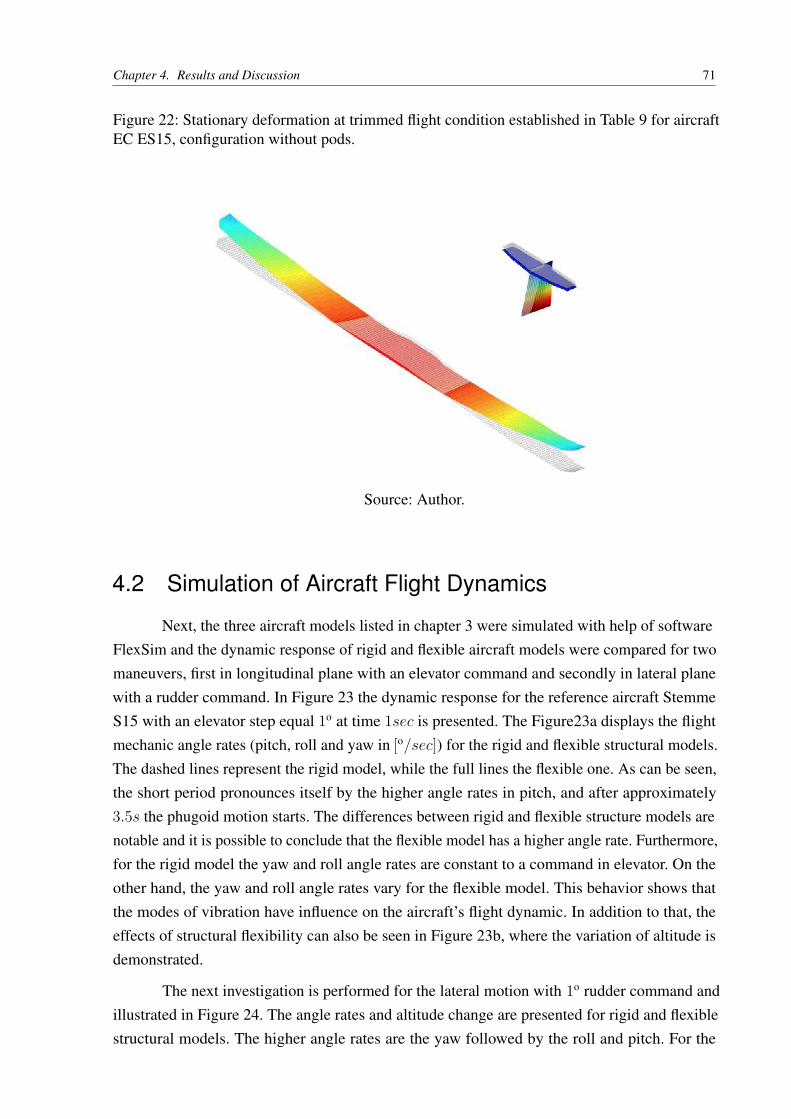
Chapter 4. Results and Discussion 71
Figure 22: Stationary deformation at trimmed flight condition established in Table 9 for aircraftEC ES15, configuration without pods.
Source: Author.
4.2 Simulation of Aircraft Flight Dynamics
Next, the three aircraft models listed in chapter 3 were simulated with help of softwareFlexSim and the dynamic response of rigid and flexible aircraft models were compared for twomaneuvers, first in longitudinal plane with an elevator command and secondly in lateral planewith a rudder command. In Figure 23 the dynamic response for the reference aircraft StemmeS15 with an elevator step equal 1o at time 1sec is presented. The Figure23a displays the flightmechanic angle rates (pitch, roll and yaw in [o/sec]) for the rigid and flexible structural models.The dashed lines represent the rigid model, while the full lines the flexible one. As can be seen,the short period pronounces itself by the higher angle rates in pitch, and after approximately3.5s the phugoid motion starts. The differences between rigid and flexible structure models arenotable and it is possible to conclude that the flexible model has a higher angle rate. Furthermore,for the rigid model the yaw and roll angle rates are constant to a command in elevator. On theother hand, the yaw and roll angle rates vary for the flexible model. This behavior shows thatthe modes of vibration have influence on the aircraft’s flight dynamic. In addition to that, theeffects of structural flexibility can also be seen in Figure 23b, where the variation of altitude isdemonstrated.
The next investigation is performed for the lateral motion with 1o rudder command andillustrated in Figure 24. The angle rates and altitude change are presented for rigid and flexiblestructural models. The higher angle rates are the yaw followed by the roll and pitch. For the
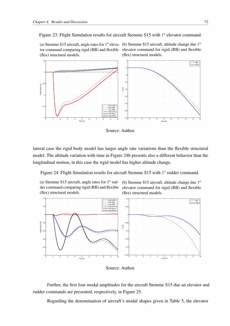
Chapter 4. Results and Discussion 72
Figure 23: Flight Simulation results for aircraft Stemme S15 with 1o elevator command.
(a) Stemme S15 aircraft, angle rates for 1o eleva-tor command comparing rigid (RB) and flexible(flex) structural models.
0 1 2 3 4 5 6 7 8 9 10−2
−1.5
−1
−0.5
0
0.5
Time (s)
Ang
le R
ate
(º/s
)
Pitch (RB)Roll (RB)Yaw (RB)Pitch (Flex)Roll (Flex)Yaw (Flex)
(b) Stemme S15 aircraft, altitude change due 1o
elevator command for rigid (RB) and flexible(flex) structural models.
0 1 2 3 4 5 6 7 8 9 10−35
−30
−25
−20
−15
−10
−5
0
5
Time (s)H
(m
)
RBFlex
Source: Author.
lateral case the rigid body model has larger angle rate variations than the flexible structuralmodel. The altitude variation with time in Figure 24b presents also a different behavior than thelongitudinal motion, in this case the rigid model has higher altitude change.
Figure 24: Flight Simulation results for aircraft Stemme S15 with 1o rudder command.
(a) Stemme S15 aircraft, angle rates for 1o rud-der command comparing rigid (RB) and flexible(flex) structural models.
0 1 2 3 4 5 6 7 8 9 10−1
−0.8
−0.6
−0.4
−0.2
0
0.2
0.4
Time (s)
Ang
le R
ate
(º/s
)
Pitch (RB)Roll (RB)Yaw (RB)Pitch (Flex)Roll (Flex)Yaw (Flex)
(b) Stemme S15 aircraft, altitude change due 1o
elevator command for rigid (RB) and flexible(flex) structural models.
0 1 2 3 4 5 6 7 8 9 10−0.25
−0.2
−0.15
−0.1
−0.05
0
0.05
0.1
Time (s)
H (
m)
RBFlex
Source: Author.
Further, the first four modal amplitudes for the aircraft Stemme S15 due an elevator andrudder commands are presented, respectively, in Figure 25.
Regarding the denomination of aircraft’s modal shapes given in Table 5, the elevator
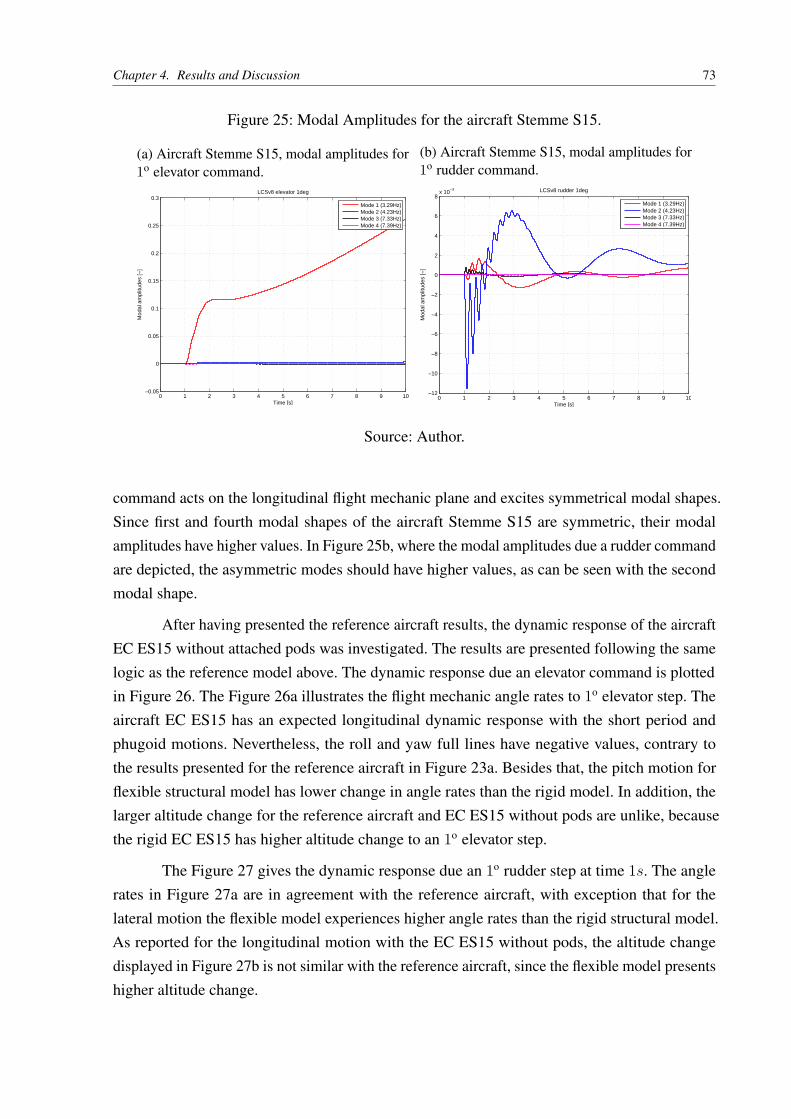
Chapter 4. Results and Discussion 73
Figure 25: Modal Amplitudes for the aircraft Stemme S15.
(a) Aircraft Stemme S15, modal amplitudes for1o elevator command.
0 1 2 3 4 5 6 7 8 9 10−0.05
0
0.05
0.1
0.15
0.2
0.25
0.3
Time [s]
Mod
al a
mpl
itude
s [−
]
LCSv8 elevator 1deg
Mode 1 (3.29Hz)Mode 2 (4.23Hz)Mode 3 (7.33Hz)Mode 4 (7.39Hz)
(b) Aircraft Stemme S15, modal amplitudes for1o rudder command.
0 1 2 3 4 5 6 7 8 9 10−12
−10
−8
−6
−4
−2
0
2
4
6
8x 10
−3
Time [s]
Mod
al a
mpl
itude
s [−
]
LCSv8 rudder 1deg
Mode 1 (3.29Hz)Mode 2 (4.23Hz)Mode 3 (7.33Hz)Mode 4 (7.39Hz)
Source: Author.
command acts on the longitudinal flight mechanic plane and excites symmetrical modal shapes.Since first and fourth modal shapes of the aircraft Stemme S15 are symmetric, their modalamplitudes have higher values. In Figure 25b, where the modal amplitudes due a rudder commandare depicted, the asymmetric modes should have higher values, as can be seen with the secondmodal shape.
After having presented the reference aircraft results, the dynamic response of the aircraftEC ES15 without attached pods was investigated. The results are presented following the samelogic as the reference model above. The dynamic response due an elevator command is plottedin Figure 26. The Figure 26a illustrates the flight mechanic angle rates to 1o elevator step. Theaircraft EC ES15 has an expected longitudinal dynamic response with the short period andphugoid motions. Nevertheless, the roll and yaw full lines have negative values, contrary tothe results presented for the reference aircraft in Figure 23a. Besides that, the pitch motion forflexible structural model has lower change in angle rates than the rigid model. In addition, thelarger altitude change for the reference aircraft and EC ES15 without pods are unlike, becausethe rigid EC ES15 has higher altitude change to an 1o elevator step.
The Figure 27 gives the dynamic response due an 1o rudder step at time 1s. The anglerates in Figure 27a are in agreement with the reference aircraft, with exception that for thelateral motion the flexible model experiences higher angle rates than the rigid structural model.As reported for the longitudinal motion with the EC ES15 without pods, the altitude changedisplayed in Figure 27b is not similar with the reference aircraft, since the flexible model presentshigher altitude change.
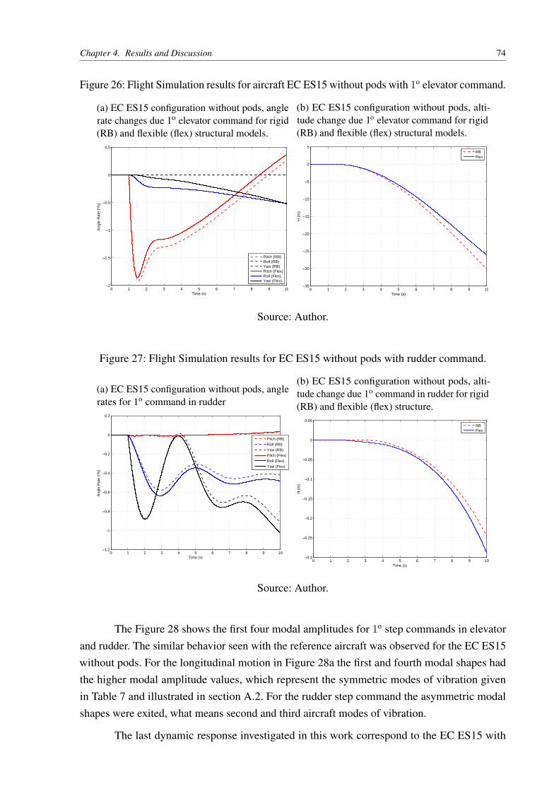
Chapter 4. Results and Discussion 74
Figure 26: Flight Simulation results for aircraft EC ES15 without pods with 1o elevator command.
(a) EC ES15 configuration without pods, anglerate changes due 1o elevator command for rigid(RB) and flexible (flex) structural models.
0 1 2 3 4 5 6 7 8 9 10−2
−1.5
−1
−0.5
0
0.5
Time (s)
Ang
le R
ate
(º/s
)
Pitch (RB)Roll (RB)Yaw (RB)Pitch (Flex)Roll (Flex)Yaw (Flex)
(b) EC ES15 configuration without pods, alti-tude change due 1o elevator command for rigid(RB) and flexible (flex) structural models.
0 1 2 3 4 5 6 7 8 9 10−35
−30
−25
−20
−15
−10
−5
0
5
Time (s)H
(m
)
RBFlex
Source: Author.
Figure 27: Flight Simulation results for EC ES15 without pods with rudder command.
(a) EC ES15 configuration without pods, anglerates for 1o command in rudder
0 1 2 3 4 5 6 7 8 9 10−1.2
−1
−0.8
−0.6
−0.4
−0.2
0
0.2
Time (s)
Ang
le R
ate
(º/s
)
Pitch (RB)
Roll (RB)
Yaw (RB)
Pitch (Flex)
Roll (Flex)
Yaw (Flex)
(b) EC ES15 configuration without pods, alti-tude change due 1o command in rudder for rigid(RB) and flexible (flex) structure.
0 1 2 3 4 5 6 7 8 9 10−0.3
−0.25
−0.2
−0.15
−0.1
−0.05
0
0.05
Time (s)
H (
m)
RBFlex
Source: Author.
The Figure 28 shows the first four modal amplitudes for 1o step commands in elevatorand rudder. The similar behavior seen with the reference aircraft was observed for the EC ES15without pods. For the longitudinal motion in Figure 28a the first and fourth modal shapes hadthe higher modal amplitude values, which represent the symmetric modes of vibration givenin Table 7 and illustrated in section A.2. For the rudder step command the asymmetric modalshapes were exited, what means second and third aircraft modes of vibration.
The last dynamic response investigated in this work correspond to the EC ES15 with
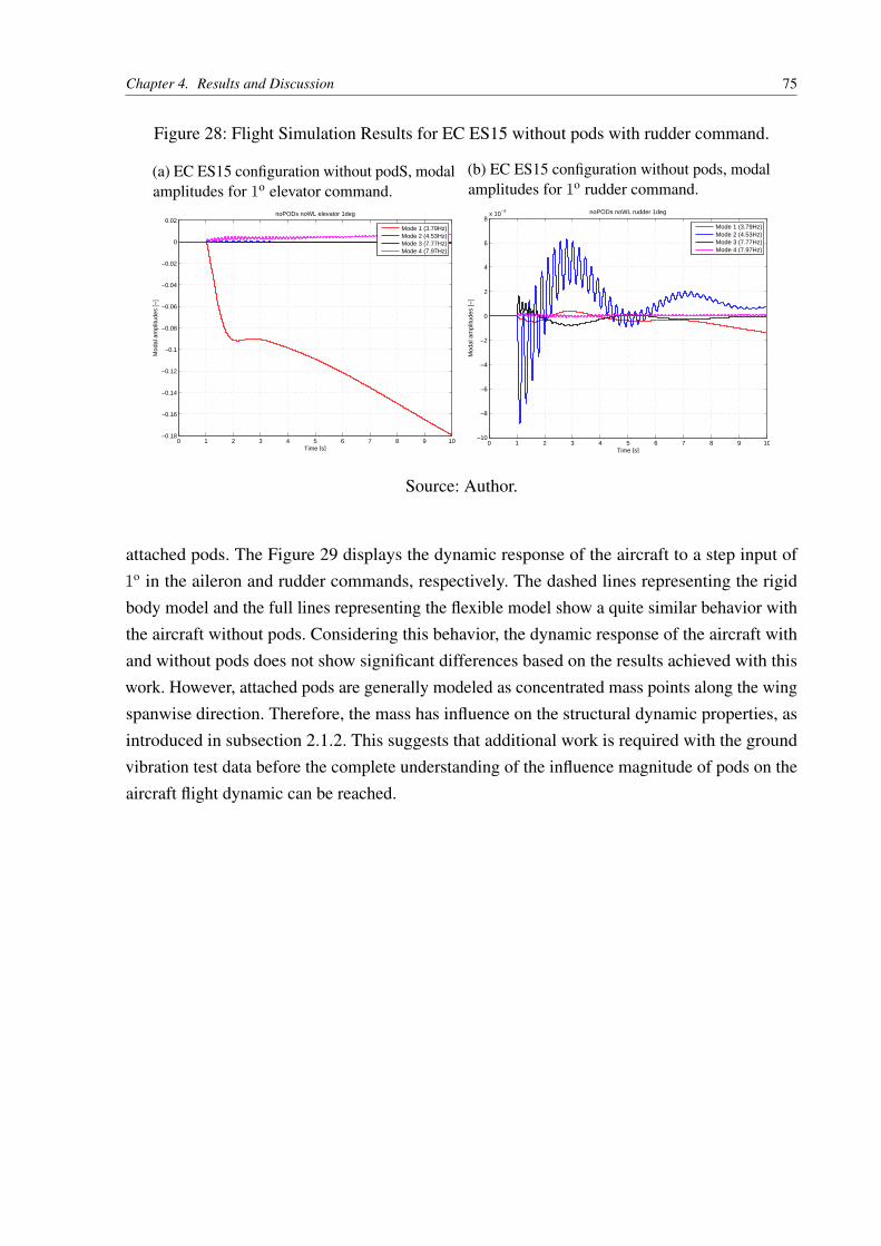
Chapter 4. Results and Discussion 75
Figure 28: Flight Simulation Results for EC ES15 without pods with rudder command.
(a) EC ES15 configuration without podS, modalamplitudes for 1o elevator command.
0 1 2 3 4 5 6 7 8 9 10−0.18
−0.16
−0.14
−0.12
−0.1
−0.08
−0.06
−0.04
−0.02
0
0.02
Time [s]
Mod
al a
mpl
itude
s [−
]
noPODs noWL elevator 1deg
Mode 1 (3.79Hz)Mode 2 (4.53Hz)Mode 3 (7.77Hz)Mode 4 (7.97Hz)
(b) EC ES15 configuration without pods, modalamplitudes for 1o rudder command.
0 1 2 3 4 5 6 7 8 9 10−10
−8
−6
−4
−2
0
2
4
6
8x 10
−3
Time [s]
Mod
al a
mpl
itude
s [−
]
noPODs noWL rudder 1deg
Mode 1 (3.79Hz)Mode 2 (4.53Hz)Mode 3 (7.77Hz)Mode 4 (7.97Hz)
Source: Author.
attached pods. The Figure 29 displays the dynamic response of the aircraft to a step input of1o in the aileron and rudder commands, respectively. The dashed lines representing the rigidbody model and the full lines representing the flexible model show a quite similar behavior withthe aircraft without pods. Considering this behavior, the dynamic response of the aircraft withand without pods does not show significant differences based on the results achieved with thiswork. However, attached pods are generally modeled as concentrated mass points along the wingspanwise direction. Therefore, the mass has influence on the structural dynamic properties, asintroduced in subsection 2.1.2. This suggests that additional work is required with the groundvibration test data before the complete understanding of the influence magnitude of pods on theaircraft flight dynamic can be reached.
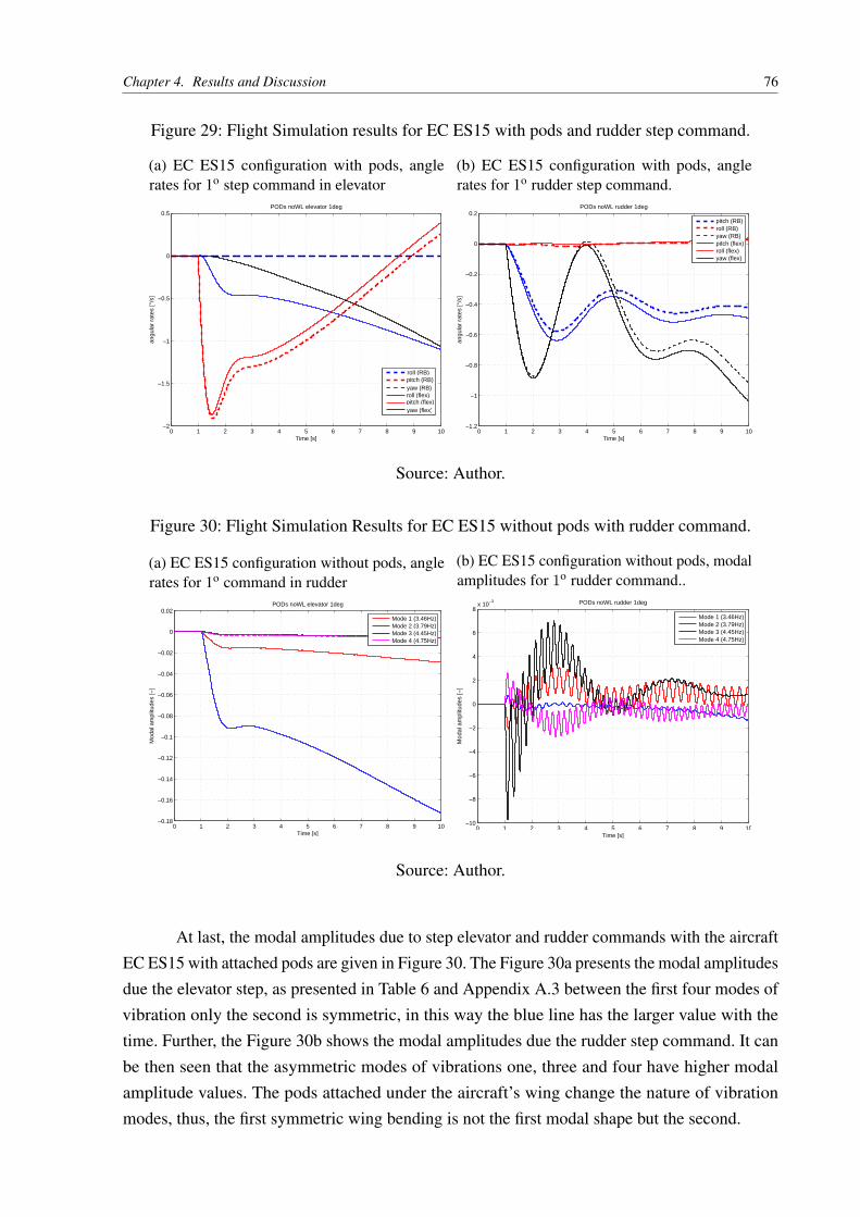
Chapter 4. Results and Discussion 76
Figure 29: Flight Simulation results for EC ES15 with pods and rudder step command.
(a) EC ES15 configuration with pods, anglerates for 1o step command in elevator
0 1 2 3 4 5 6 7 8 9 10−2
−1.5
−1
−0.5
0
0.5
Time [s]
angu
lar
rate
s [°
/s]
PODs noWL elevator 1deg
pitch (RB)roll (RB)
yaw (RB)
pitch (flex)roll (flex)
yaw (flex)
(b) EC ES15 configuration with pods, anglerates for 1o rudder step command.
0 1 2 3 4 5 6 7 8 9 10−1.2
−1
−0.8
−0.6
−0.4
−0.2
0
0.2
Time [s]
angu
lar
rate
s [°
/s]
PODs noWL rudder 1deg
pitch (RB)roll (RB)yaw (RB)pitch (flex)roll (flex)yaw (flex)
Source: Author.
Figure 30: Flight Simulation Results for EC ES15 without pods with rudder command.
(a) EC ES15 configuration without pods, anglerates for 1o command in rudder
0 1 2 3 4 5 6 7 8 9 10−0.18
−0.16
−0.14
−0.12
−0.1
−0.08
−0.06
−0.04
−0.02
0
0.02
Time [s]
Mod
al a
mpl
itude
s [−
]
PODs noWL elevator 1deg
Mode 1 (3.46Hz)Mode 2 (3.79Hz)Mode 3 (4.45Hz)Mode 4 (4.75Hz)
(b) EC ES15 configuration without pods, modalamplitudes for 1o rudder command..
0 1 2 3 4 5 6 7 8 9 10−10
−8
−6
−4
−2
0
2
4
6
8x 10
−3
Time [s]
Mod
al a
mpl
itude
s [−
]
PODs noWL rudder 1deg
Mode 1 (3.46Hz)Mode 2 (3.79Hz)Mode 3 (4.45Hz)Mode 4 (4.75Hz)
Source: Author.
At last, the modal amplitudes due to step elevator and rudder commands with the aircraftEC ES15 with attached pods are given in Figure 30. The Figure 30a presents the modal amplitudesdue the elevator step, as presented in Table 6 and Appendix A.3 between the first four modes ofvibration only the second is symmetric, in this way the blue line has the larger value with thetime. Further, the Figure 30b shows the modal amplitudes due the rudder step command. It canbe then seen that the asymmetric modes of vibrations one, three and four have higher modalamplitude values. The pods attached under the aircraft’s wing change the nature of vibrationmodes, thus, the first symmetric wing bending is not the first modal shape but the second.
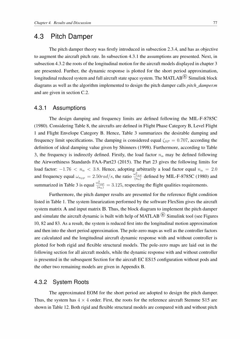
Chapter 4. Results and Discussion 77
4.3 Pitch Damper
The pitch damper theory was firstly introduced in subsection 2.3.4, and has as objectiveto augment the aircraft pitch rate. In subsection 4.3.1 the assumptions are presented. Next, insubsection 4.3.2 the roots of the longitudinal motion for the aircraft models displayed in chapter 3are presented. Further, the dynamic response is plotted for the short period approximation,longitudinal reduced system and full aircraft state space system. The MATLAB R© Simulink blockdiagrams as well as the algorithm implemented to design the pitch damper calls pitch_damper.m
and are given in section C.2.
4.3.1 Assumptions
The design damping and frequency limits are defined following the MIL-F-8785C(1980). Considering Table 8, the aircrafts are defined in Flight Phase Category B, Level Flight1 and Flight Envelope Category B. Hence, Table 3 summarizes the desirable damping andfrequency limit specifications. The damping is considered equal ζSP = 0.707, according thedefinition of ideal damping value given by Shinners (1998). Furthermore, according to Table3, the frequency is indirectly defined. Firstly, the load factor nα may be defined followingthe Airworthiness Standards FAA-Part23 (2015). The Part 23 gives the following limits forload factor: −1.76 < nα < 3.8. Hence, adopting arbitrarily a load factor equal nα = 2.0and frequency equal ωnSP = 2.50rad/s, the ratio
ω2nSP
(nα) defined by MIL-F-8785C (1980) and
summarized in Table 3 is equalω2nSP
(nα) = 3.125, respecting the flight qualities requirements.
Furthermore, the pitch damper results are presented for the reference flight conditionlisted in Table 1. The system linearization performed by the software FlexSim gives the aircraftsystem matrix A and input matrix B. Thus, the block diagram to implement the pitch damperand simulate the aircraft dynamic is built with help of MATLAB R© Simulink tool (see Figures10, 82 and 83. As a result, the system is reduced first into the longitudinal motion approximationand then into the short period approximation. The pole-zero maps as well as the controller factorsare calculated and the longitudinal aircraft dynamic response with and without controller isplotted for both rigid and flexible structural models. The pole-zero maps are laid out in thefollowing section for all aircraft models, while the dynamic response with and without controlleris presented in the subsequent Section for the aircraft EC ES15 configuration without pods andthe other two remaining models are given in Appendix B.
4.3.2 System Roots
The approximated EOM for the short period are adopted to design the pitch damper.Thus, the system has 4 × 4 order. First, the roots for the reference aircraft Stemme S15 areshown in Table 12. Both rigid and flexible structural models are compared with and without pitch
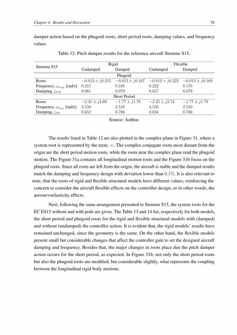
Chapter 4. Results and Discussion 78
damper action based on the phugoid roots, short period roots, damping values, and frequencyvalues.
Table 12: Pitch damper results for the reference aircraft Stemme S15.
Stemme S15Rigid Flexible
Undamped Damped Undamped DampedPhugoid
Roots −0.013± j0.215 −0.013± j0.167 −0.012 + j0.222 −0.013± j0.169Frequency, ωnPH [rad/s] 0.215 0.168 0.222 0.170Damping, ζPH 0.061 0.079 0.057 0.079
Short PeriodRoots −2.31± j2.69 −1.77± j1.78 −2.25± j2.74 −1.77± j1.78Frequency, ωnSP [rad/s] 3.550 2.510 3.550 2.510Damping, ζSP 0.652 0.706 0.634 0.706
Source: Author.
The results listed in Table 12 are also plotted in the complex-plane in Figure 31, where asystem root is represented by the term: ×. The complex conjugate roots most distant from theorigin are the short period motion roots, while the roots near the complex plane read the phugoidmotion. The Figure 31a contains all longitudinal motion roots and the Figure 31b focus on thephugoid roots. Since all roots are left from the origin, the aircraft is stable and the damped resultsmatch the damping and frequency design with deviation lower than 0.1%. It is also relevant to
note, that the roots of rigid and flexible structural models have different values, reinforcing theconcern to consider the aircraft flexible effects on the controller design, or in other words, theaeroservoelasticity effects.
Next, following the same arrangement presented to Stemme S15, the system roots for theEC ES15 without and with pods are given. The Table 13 and 14 list, respectively for both models,the short period and phugoid roots for the rigid and flexible structural models with (damped)and without (undamped) the controller action. It is evident that, the rigid models’ results haveremained unchanged, since the geometry is the same. On the other hand, the flexible modelspresent small but considerable changes that affect the controller gain to set the designed aircraftdamping and frequency. Besides that, the major changes in roots place due the pitch damperaction occurs for the short period, as expected. In Figure 31b, not only the short period rootsbut also the phugoid roots are modified, but considerable slightly, what represents the couplingbetween the longitudinal rigid body motions.
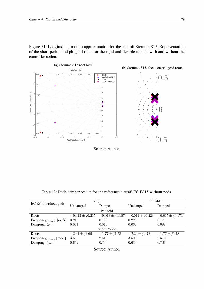
Chapter 4. Results and Discussion 79
Figure 31: Longitudinal motion approximation for the aircraft Stemme S15. Representationof the short period and phugoid roots for the rigid and flexible models with and without thecontroller action.
(a) Stemme S15 root loci.
−2.5 −2 −1.5 −1 −0.5 0 0.5−3
−2
−1
0
1
2
30.080.170.280.380.50.64
0.8
0.94
0.080.170.280.380.50.64
0.8
0.94
0.5
1
1.5
2
2.5
3
0.5
1
1.5
2
2.5
3
Pole−Zero Map
Real Axis (seconds−1)
Imag
inar
y A
xis
(sec
onds
−1 )
RIGIDRIGID DAMPEDFLEXFLEX DAMPED
(b) Stemme S15, focus on phugoid roots.
0.5
0 5
0.5
0.5
0
Source: Author.
Table 13: Pitch damper results for the reference aircraft EC ES15 without pods.
EC ES15 without podsRigid Flexible
Undamped Damped Undamped DampedPhugoid
Roots −0.013± j0.215 −0.013± j0.167 −0.014 + j0.223 −0.015± j0.171Frequency, ωnPH [rad/s] 0.215 0.168 0.223 0.171Damping, ζPH 0.061 0.079 0.062 0.088
Short PeriodRoots −2.31± j2.69 −1.77± j1.78 −2.20± j2.72 −1.77± j1.78Frequency, ωnSP [rad/s] 3.550 2.510 3.500 2.510Damping, ζSP 0.652 0.706 0.630 0.706
Source: Author.
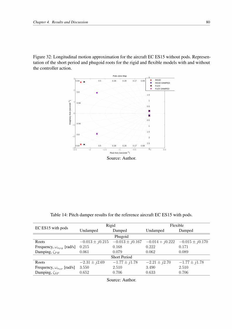
Chapter 4. Results and Discussion 80
Figure 32: Longitudinal motion approximation for the aircraft EC ES15 without pods. Represen-tation of the short period and phugoid roots for the rigid and flexible models with and withoutthe controller action.
−2.5 −2 −1.5 −1 −0.5 0 0.5−3
−2
−1
0
1
2
30.080.170.280.380.50.64
0.8
0.94
0.080.170.280.380.50.64
0.8
0.94
0.5
1
1.5
2
2.5
3
0.5
1
1.5
2
2.5
3
Pole−Zero Map
Real Axis (seconds−1)
Imag
inar
y A
xis
(sec
onds
−1 )
RIGID
RIGID DAMPED
FLEX
FLEX DAMPED
Source: Author.
Table 14: Pitch damper results for the reference aircraft EC ES15 with pods.
EC ES15 with podsRigid Flexible
Undamped Damped Undamped DampedPhugoid
Roots −0.013± j0.215 −0.013± j0.167 −0.014 + j0.222 −0.015± j0.170Frequency, ωnPH [rad/s] 0.215 0.168 0.222 0.171Damping, ζPH 0.061 0.079 0.062 0.089
Short PeriodRoots −2.31± j2.69 −1.77± j1.78 −2.21± j2.70 −1.77± j1.78Frequency, ωnSP [rad/s] 3.550 2.510 3.490 2.510Damping, ζSP 0.652 0.706 0.633 0.706
Source: Author.
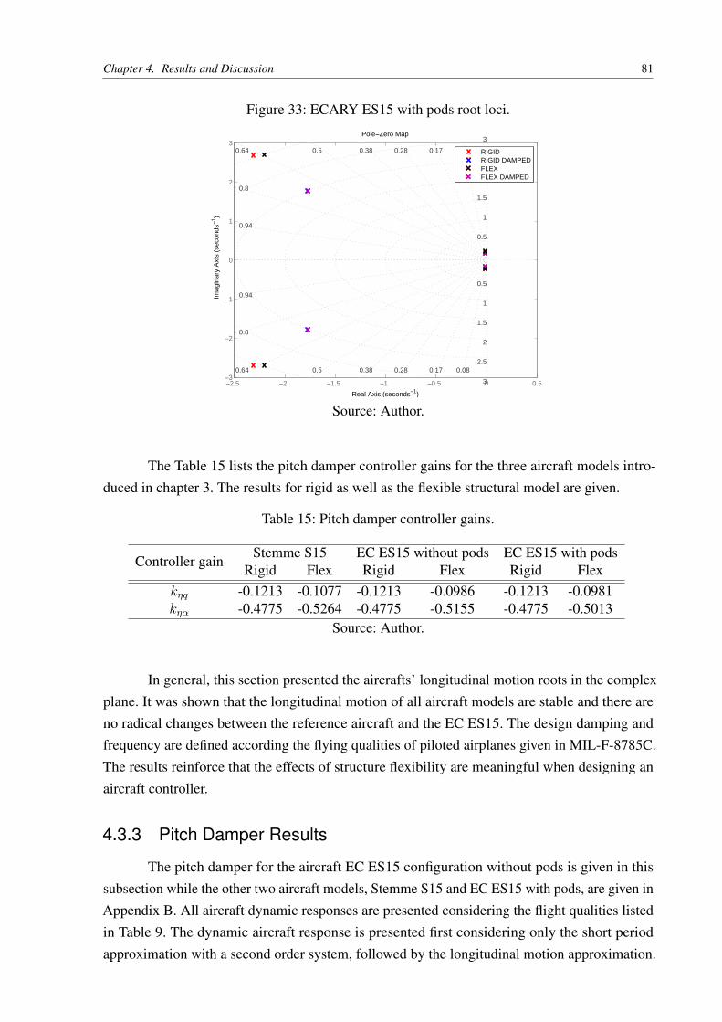
Chapter 4. Results and Discussion 81
Figure 33: ECARY ES15 with pods root loci.
−2.5 −2 −1.5 −1 −0.5 0 0.5−3
−2
−1
0
1
2
30.080.170.280.380.50.64
0.8
0.94
0.080.170.280.380.50.64
0.8
0.94
0.5
1
1.5
2
2.5
3
0.5
1
1.5
2
2.5
3
Pole−Zero Map
Real Axis (seconds−1)
Imag
inar
y A
xis
(sec
onds
−1 )
RIGIDRIGID DAMPEDFLEXFLEX DAMPED
Source: Author.
The Table 15 lists the pitch damper controller gains for the three aircraft models intro-duced in chapter 3. The results for rigid as well as the flexible structural model are given.
Table 15: Pitch damper controller gains.
Controller gainStemme S15 EC ES15 without pods EC ES15 with pods
Rigid Flex Rigid Flex Rigid Flexkηq -0.1213 -0.1077 -0.1213 -0.0986 -0.1213 -0.0981kηα -0.4775 -0.5264 -0.4775 -0.5155 -0.4775 -0.5013
Source: Author.
In general, this section presented the aircrafts’ longitudinal motion roots in the complexplane. It was shown that the longitudinal motion of all aircraft models are stable and there areno radical changes between the reference aircraft and the EC ES15. The design damping andfrequency are defined according the flying qualities of piloted airplanes given in MIL-F-8785C.The results reinforce that the effects of structure flexibility are meaningful when designing anaircraft controller.
4.3.3 Pitch Damper Results
The pitch damper for the aircraft EC ES15 configuration without pods is given in thissubsection while the other two aircraft models, Stemme S15 and EC ES15 with pods, are given inAppendix B. All aircraft dynamic responses are presented considering the flight qualities listedin Table 9. The dynamic aircraft response is presented first considering only the short periodapproximation with a second order system, followed by the longitudinal motion approximation.
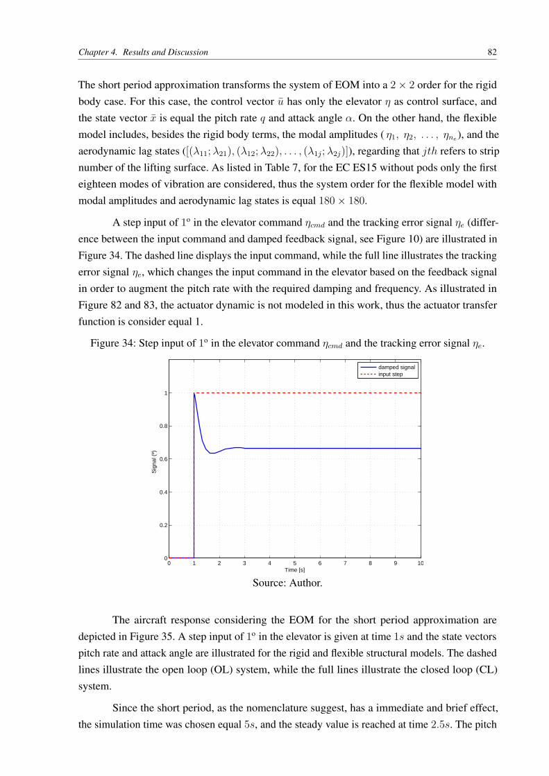
Chapter 4. Results and Discussion 82
The short period approximation transforms the system of EOM into a 2× 2 order for the rigidbody case. For this case, the control vector u has only the elevator η as control surface, andthe state vector x is equal the pitch rate q and attack angle α. On the other hand, the flexiblemodel includes, besides the rigid body terms, the modal amplitudes ( η1, η2, . . . , ηne), and theaerodynamic lag states ([(λ11;λ21), (λ12;λ22), . . . , (λ1j;λ2j)]), regarding that jth refers to stripnumber of the lifting surface. As listed in Table 7, for the EC ES15 without pods only the firsteighteen modes of vibration are considered, thus the system order for the flexible model withmodal amplitudes and aerodynamic lag states is equal 180× 180.
A step input of 1o in the elevator command ηcmd and the tracking error signal ηe (differ-ence between the input command and damped feedback signal, see Figure 10) are illustrated inFigure 34. The dashed line displays the input command, while the full line illustrates the trackingerror signal ηe, which changes the input command in the elevator based on the feedback signalin order to augment the pitch rate with the required damping and frequency. As illustrated inFigure 82 and 83, the actuator dynamic is not modeled in this work, thus the actuator transferfunction is consider equal 1.
Figure 34: Step input of 1o in the elevator command ηcmd and the tracking error signal ηe.
0 1 2 3 4 5 6 7 8 9 100
0.2
0.4
0.6
0.8
1
Time [s]
Sig
nal (
º)
damped signalinput step
Source: Author.
The aircraft response considering the EOM for the short period approximation aredepicted in Figure 35. A step input of 1o in the elevator is given at time 1s and the state vectorspitch rate and attack angle are illustrated for the rigid and flexible structural models. The dashedlines illustrate the open loop (OL) system, while the full lines illustrate the closed loop (CL)system.
Since the short period, as the nomenclature suggest, has a immediate and brief effect,the simulation time was chosen equal 5s, and the steady value is reached at time 2.5s. The pitch
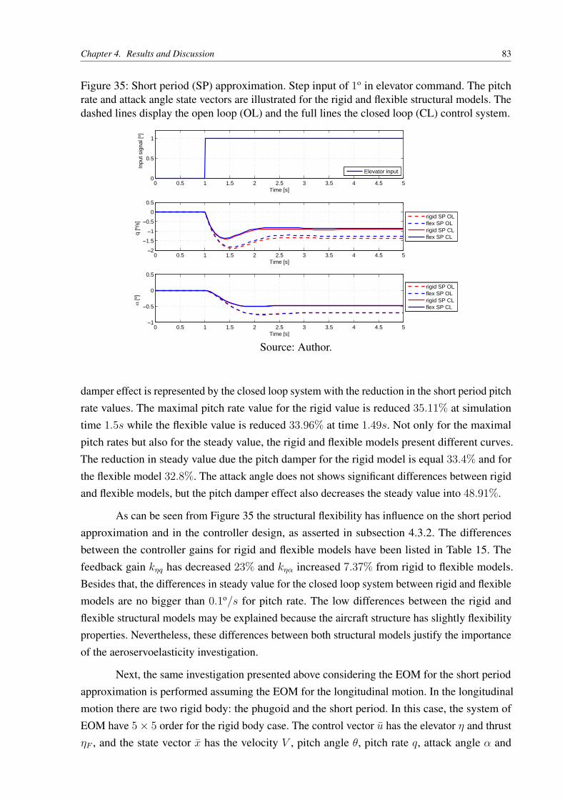
Chapter 4. Results and Discussion 83
Figure 35: Short period (SP) approximation. Step input of 1o in elevator command. The pitchrate and attack angle state vectors are illustrated for the rigid and flexible structural models. Thedashed lines display the open loop (OL) and the full lines the closed loop (CL) control system.
0 0.5 1 1.5 2 2.5 3 3.5 4 4.5 50
0.5
1
Time [s]
Inpu
t sig
nal [
º]
Elevator input
0 0.5 1 1.5 2 2.5 3 3.5 4 4.5 5−2
−1.5
−1
−0.5
0
0.5
Time [s]
q [º
/s]
rigid SP OLflex SP OLrigid SP CLflex SP CL
0 0.5 1 1.5 2 2.5 3 3.5 4 4.5 5−1
−0.5
0
0.5
Time [s]
α[º
]
rigid SP OLflex SP OLrigid SP CLflex SP CL
Source: Author.
damper effect is represented by the closed loop system with the reduction in the short period pitchrate values. The maximal pitch rate value for the rigid value is reduced 35.11% at simulationtime 1.5s while the flexible value is reduced 33.96% at time 1.49s. Not only for the maximalpitch rates but also for the steady value, the rigid and flexible models present different curves.The reduction in steady value due the pitch damper for the rigid model is equal 33.4% and forthe flexible model 32.8%. The attack angle does not shows significant differences between rigidand flexible models, but the pitch damper effect also decreases the steady value into 48.91%.
As can be seen from Figure 35 the structural flexibility has influence on the short periodapproximation and in the controller design, as asserted in subsection 4.3.2. The differencesbetween the controller gains for rigid and flexible models have been listed in Table 15. Thefeedback gain kηq has decreased 23% and kηα increased 7.37% from rigid to flexible models.Besides that, the differences in steady value for the closed loop system between rigid and flexiblemodels are no bigger than 0.1o/s for pitch rate. The low differences between the rigid andflexible structural models may be explained because the aircraft structure has slightly flexibilityproperties. Nevertheless, these differences between both structural models justify the importanceof the aeroservoelasticity investigation.
Next, the same investigation presented above considering the EOM for the short periodapproximation is performed assuming the EOM for the longitudinal motion. In the longitudinalmotion there are two rigid body: the phugoid and the short period. In this case, the system ofEOM have 5× 5 order for the rigid body case. The control vector u has the elevator η and thrustηF , and the state vector x has the velocity V , pitch angle θ, pitch rate q, attack angle α and
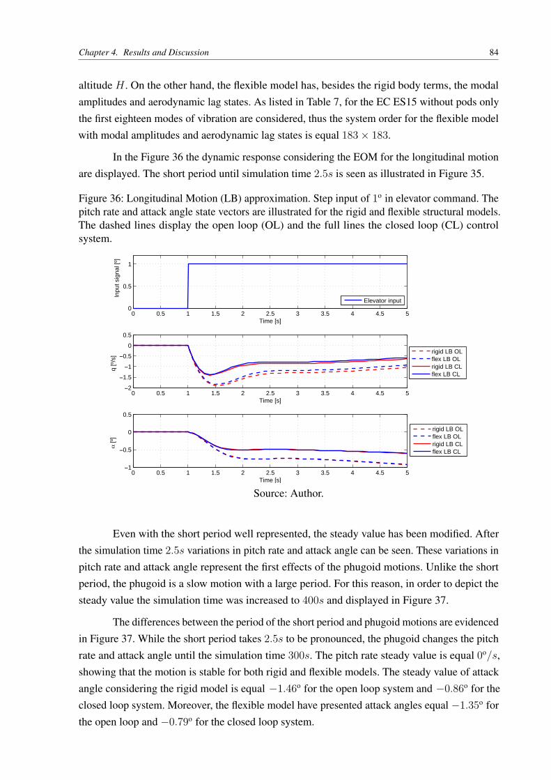
Chapter 4. Results and Discussion 84
altitude H . On the other hand, the flexible model has, besides the rigid body terms, the modalamplitudes and aerodynamic lag states. As listed in Table 7, for the EC ES15 without pods onlythe first eighteen modes of vibration are considered, thus the system order for the flexible modelwith modal amplitudes and aerodynamic lag states is equal 183× 183.
In the Figure 36 the dynamic response considering the EOM for the longitudinal motionare displayed. The short period until simulation time 2.5s is seen as illustrated in Figure 35.
Figure 36: Longitudinal Motion (LB) approximation. Step input of 1o in elevator command. Thepitch rate and attack angle state vectors are illustrated for the rigid and flexible structural models.The dashed lines display the open loop (OL) and the full lines the closed loop (CL) controlsystem.
0 0.5 1 1.5 2 2.5 3 3.5 4 4.5 50
0.5
1
Time [s]
Inpu
t sig
nal [
º]
Elevator input
0 0.5 1 1.5 2 2.5 3 3.5 4 4.5 5−2
−1.5
−1
−0.5
0
0.5
Time [s]
q [º
/s]
rigid LB OLflex LB OLrigid LB CLflex LB CL
0 0.5 1 1.5 2 2.5 3 3.5 4 4.5 5−1
−0.5
0
0.5
Time [s]
α[º
]
rigid LB OLflex LB OLrigid LB CLflex LB CL
Source: Author.
Even with the short period well represented, the steady value has been modified. Afterthe simulation time 2.5s variations in pitch rate and attack angle can be seen. These variations inpitch rate and attack angle represent the first effects of the phugoid motions. Unlike the shortperiod, the phugoid is a slow motion with a large period. For this reason, in order to depict thesteady value the simulation time was increased to 400s and displayed in Figure 37.
The differences between the period of the short period and phugoid motions are evidencedin Figure 37. While the short period takes 2.5s to be pronounced, the phugoid changes the pitchrate and attack angle until the simulation time 300s. The pitch rate steady value is equal 0o/s,showing that the motion is stable for both rigid and flexible models. The steady value of attackangle considering the rigid model is equal −1.46o for the open loop system and −0.86o for theclosed loop system. Moreover, the flexible model have presented attack angles equal −1.35o forthe open loop and −0.79o for the closed loop system.
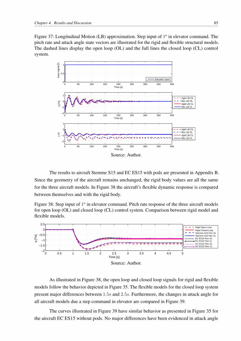
Chapter 4. Results and Discussion 85
Figure 37: Longitudinal Motion (LB) approximation. Step input of 1o in elevator command. Thepitch rate and attack angle state vectors are illustrated for the rigid and flexible structural models.The dashed lines display the open loop (OL) and the full lines the closed loop (CL) controlsystem.
0 50 100 150 200 250 300 350 4000
0.5
1
Time [s]
Inpu
t sig
nal [
º]
Elevator input
0 50 100 150 200 250 300 350 400−2
−1
0
1
Time [s]
q [º
/s]
rigid LB OLflex LB OLrigid LB CLflex LB CL
0 50 100 150 200 250 300 350 400
−2
−1
0
1
Time [s]
α[º
]
rigid LB OLflex LB OLrigid LB CLflex LB CL
Source: Author.
The results to aircraft Stemme S15 and EC ES15 with pods are presented in Appendix B.Since the geometry of the aircraft remains unchanged, the rigid body values are all the samefor the three aircraft models. In Figure 38 the aircraft’s flexible dynamic response is comparedbetween themselves and with the rigid body.
Figure 38: Step input of 1o in elevator command. Pitch rate response of the three aircraft modelsfor open loop (OL) and closed loop (CL) control system. Comparison between rigid model andflexible models.
0 0.5 1 1.5 2 2.5 3 3.5 4 4.5 5−2
−1.5
−1
−0.5
0
0.5
Time [s]
q [º
/s]
Rigid Open Loop
Stemme S15 Flex OLRigid Closed Loop
Stemme S15 Flex CLEC ES15 Flex OLEC ES15 Flex CLEC ES15 Flex OLEC ES15 Flex CL
Source: Author.
As illustrated in Figure 38, the open loop and closed loop signals for rigid and flexiblemodels follow the behavior depicted in Figure 35. The flexible models for the closed loop systempresent major differences between 1.5s and 2.5s. Furthermore, the changes in attack angle forall aircraft models due a step command in elevator are compared in Figure 39.
The curves illustrated in Figure 39 have similar behavior as presented in Figure 35 forthe aircraft EC ES15 without pods. No major differences have been evidenced in attack angle
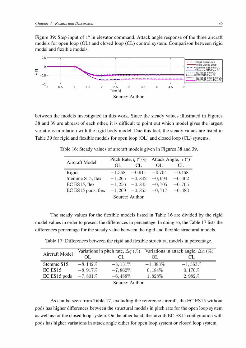
Chapter 4. Results and Discussion 86
Figure 39: Step input of 1o in elevator command. Attack angle response of the three aircraftmodels for open loop (OL) and closed loop (CL) control system. Comparison between rigidmodel and flexible models.
0 0.5 1 1.5 2 2.5 3 3.5 4 4.5 5−1
−0.5
0
0.5
Time [s]
α[º
]
Rigid Open LoopRigid Closed LoopStemme S15 Flex OLStemme S15 Flex CLEC ES15 Flex OLEC ES15 Flex CLEC ES15 pods Flex OLEC ES15 pods Flex CL
Source: Author.
between the models investigated in this work. Since the steady values illustrated in Figures38 and 39 are abreast of each other, it is difficult to point out which model gives the largestvariations in relation with the rigid body model. Due this fact, the steady values are listed inTable 39 for rigid and flexible models for open loop (OL) and closed loop (CL) systems.
Table 16: Steady values of aircraft models given in Figures 38 and 39.
Aircraft ModelPitch Rate, q (o/s) Attack Angle, α (o)
OL CL OL CLRigid −1.368 −0.911 −0.704 −0.468Stemme S15, flex −1, 265 −0, 842 −0, 694 −0, 462EC ES15, flex −1, 256 −0, 845 −0, 705 −0, 705EC ES15 pods, flex −1, 269 −0, 855 −0, 717 −0, 483
Source: Author.
The steady values for the flexible models listed in Table 16 are divided by the rigidmodel values in order to present the differences in percentage. In doing so, the Table 17 lists thedifferences percentage for the steady value between the rigid and flexible structural models.
Table 17: Differences between the rigid and flexible structural models in percentage.
Aircraft ModelVariations in pitch rate, ∆q (%) Variations in attack angle, ∆α (%)
OL CL OL CLStemme S15 −8, 142% −8, 131% −1, 383% −1, 363%EC ES15 −8, 917% −7, 862% 0, 184% 0, 170%EC ES15 pods −7, 801% −6, 488% 1, 828% 2, 982%
Source: Author.
As can be seen from Table 17, excluding the reference aircraft, the EC ES15 withoutpods has higher differences between the structural models in pitch rate for the open loop systemas well as for the closed loop system. On the other hand, the aircraft EC ES15 configuration withpods has higher variations in attack angle either for open loop system or closed loop system.
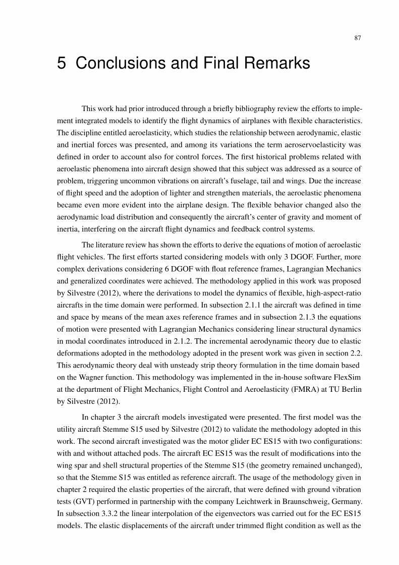
87
5 Conclusions and Final Remarks
This work had prior introduced through a briefly bibliography review the efforts to imple-ment integrated models to identify the flight dynamics of airplanes with flexible characteristics.The discipline entitled aeroelasticity, which studies the relationship between aerodynamic, elasticand inertial forces was presented, and among its variations the term aeroservoelasticity wasdefined in order to account also for control forces. The first historical problems related withaeroelastic phenomena into aircraft design showed that this subject was addressed as a source ofproblem, triggering uncommon vibrations on aircraft’s fuselage, tail and wings. Due the increaseof flight speed and the adoption of lighter and strengthen materials, the aeroelastic phenomenabecame even more evident into the airplane design. The flexible behavior changed also theaerodynamic load distribution and consequently the aircraft’s center of gravity and moment ofinertia, interfering on the aircraft flight dynamics and feedback control systems.
The literature review has shown the efforts to derive the equations of motion of aeroelasticflight vehicles. The first efforts started considering models with only 3 DGOF. Further, morecomplex derivations considering 6 DGOF with float reference frames, Lagrangian Mechanicsand generalized coordinates were achieved. The methodology applied in this work was proposedby Silvestre (2012), where the derivations to model the dynamics of flexible, high-aspect-ratioaircrafts in the time domain were performed. In subsection 2.1.1 the aircraft was defined in timeand space by means of the mean axes reference frames and in subsection 2.1.3 the equationsof motion were presented with Lagrangian Mechanics considering linear structural dynamicsin modal coordinates introduced in 2.1.2. The incremental aerodynamic theory due to elasticdeformations adopted in the methodology adopted in the present work was given in section 2.2.This aerodynamic theory deal with unsteady strip theory formulation in the time domain basedon the Wagner function. This methodology was implemented in the in-house software FlexSimat the department of Flight Mechanics, Flight Control and Aeroelasticity (FMRA) at TU Berlinby Silvestre (2012).
In chapter 3 the aircraft models investigated were presented. The first model was theutility aircraft Stemme S15 used by Silvestre (2012) to validate the methodology adopted in thiswork. The second aircraft investigated was the motor glider EC ES15 with two configurations:with and without attached pods. The aircraft EC ES15 was the result of modifications into thewing spar and shell structural properties of the Stemme S15 (the geometry remained unchanged),so that the Stemme S15 was entitled as reference aircraft. The usage of the methodology given inchapter 2 required the elastic properties of the aircraft, that were defined with ground vibrationtests (GVT) performed in partnership with the company Leichtwerk in Braunschweig, Germany.In subsection 3.3.2 the linear interpolation of the eigenvectors was carried out for the EC ES15models. The elastic displacements of the aircraft under trimmed flight condition as well as the
Chapter 5. Conclusions and Final Remarks 88
flight dynamic response and aircraft system matrix necessary to implement the pitch damperwere introduced.
In chapter 4 the flight dynamic response and pitch damper implementation results werepresented. The aircraft geometry, position of elastic axis, control surfaces and structural andaerodynamic models of the aircraft, the trimmed condition as well as the linearized model andthe flight dynamic simulations were obtained working with the software FlexSim. In section 4.1the trimmed flight condition obtained with the structural model from the modal operationalanalysis was not satisfactory because the controls aileron and ruder have presented significantnon symmetric values. For this reason, the eigenvectors were investigated in order to find apossible inconsistence. The contribution of each modal shape into modal amplitudes and trimparameters was investigated. The first symmetric wing bending and the first asymmetric wingtorsion were corrected by multiplying the torsion component per zero and 1.5 factors, respectively,for the configuration without pods. The same investigation was carried out for the configurationwith pods and five modal shapes were corrected. After the fixing of eigenvectors the correctedstructural properties of both EC ES15 configurations still presented asymmetric trimmed flightdue an elevator input but not so critical as previous. With the corrected trimmed values the modelwas linearized and the system matrix was obtained.
Further, in section 4.2 the flight dynamic response of aircraft models introduced inchapter 3 was carried out. The aircraft models were simulated with classical flight mechanicsconsidering the structure as a rigid-body and also with flexible linear structural dynamics. Theresponse was presented for two distinguish maneuvers, the first comprehended a step input of 1o
in the elevator and second a step input of 1o in the rudder. The elevator command was definedto investigate the longitudinal flight dynamic angle rates, specially the pitch rate. On the otherhand, the step in rudder was carried out in order to see most the lateral motion angle rates. Thedifferences between the rigid-body and flexible approach could be clearly seen, due the factthat the angle rates are modified due the flexibility effects. The comparison between the twoaircraft has showed differences between the Stemme S15 and both EC ES15 configurations. Ingeneral, in the longitudinal motion the rigid body model of aircraft EC ES15 has higher anglerates than the flexible model, while the Stemme S15 has presented inverse results. Next, in thelateral motion both EC ES15 configurations have higher yaw rates for the flexible than the rigidbody model, and the Stemme S15 presented higher yaw rates for the rigid body. No relevantdifferences between the configurations of EC ES15 were identified. Besides that, the modalamplitudes of the first four modal shapes with its respective frequencies were plotted. It hasbeen possible to see that the elevator commands had excited mostly the symmetric modes ofvibration, while the rudder command the lateral ones. Unlike the Stemme S15 and EC ES15without pods, the EC configuration with pods had the first wing symmetric bending modal shapeas the second mode of vibration instead of the first. This fact has well demonstrated the effectsof control inputs on the modal amplitudes excitation.
Chapter 5. Conclusions and Final Remarks 89
The linearized EOM in state space arrangement had able to implement the pitch damper.Due simplification the actuator dynamics was not modeled in this work. The design frequencyand damping were defined following the military specifications MIL-F-8785C. The longitudinaland short period motion approximation were performed with help of MATLABR© and the openand closed loop block diagrams were created with the Simulink tool. The open and closed loopresponses were compared for rigid body and flexible structural model, as well. The feedbackloop augmented the damping of the system reducing the effect of the pitch rates variations in theshort period motion and improving the flight comfort. The comparison between the Ecarys ES15models showed that for the configuration without pods higher differences between the rigid andflexible structural models in pitch rates for the open loop system as well as for the closed loopsystem are seen. On the other hand, the configuration with pods had higher variation in attackangle either for the open loop system or for the closed loop system. Besides that, even with theaircrafts not presenting higher differences between themselves, the effects of structural flexibilityhad influence on the controller gains as well as on the steady and maximum values.
5.1 Final Remarks
This work applied a methodology to model the dynamics of flexible, high-aspect-ratioaircraft in time domain to identify the dynamic response of the utility aircraft EC ES15 with andwithout attached pods. The structural dynamic properties of the aircraft were defined by meansof eigenvectors from ground vibrations tests. These eigenvectors were linear interpolated overthe aircraft geometry and the modes of vibration could be represented. The rigid body as well asthe flexible structure dynamics were investigated and its influence on the flight dynamic anglerates were plotted for input steps in elevator and rudder controls. The results obtained with thiswork showed that they are in good agreement with the reference aircraft Stemme S15. The pitchdamper was designed following the military specifications for piloted aircrafts and dampingthe pitch rate. High differences were not observed between the rigid body and flexible models.Nevertheless, the effects of the aircraft flexibility changed the flight dynamic response and thecontrol gains, proving that for high fidelity feedback systems, to include the flexibility effects ofthe aircraft structure is a recommended measure.
5.2 Future Works
Although the results presented here have demonstrated not only the effectiveness of themethodology and the pitch damper, but also the relevance of to consider the effects of structuralflexibility on the aircraft flight dynamics, the following activities could be developed in futureworks:
• Since the effect of pods into the flight dynamics was not significantly shown, a detailed

Chapter 5. Conclusions and Final Remarks 90
investigation of the pods’ effects on the aircraft dynamics would be interesting;
• The consideration of the wing let effects on the aerodynamic and structural models;
• Since the structural properties of the aircraft were obtained based only in GVTs, a FEMcould be carried out to compare the results;
• In the pitch damper design, to model the actuator dynamics as a electric servo-motorto identify the dead time and optimize the parameters for the elastic models by usingMulti-Objective Parameters Synthesis with the software MOPS (JOOS, 2002), for instance;
• Investigation of different flight phases varying the flight speed in order to identify theflutter speeds with the k−method;
91
Bibliography
ANDERSON, J. D. Fundamentals of Aerodynamics. 5. ed. New York, USA: McGraw-Hill,2010. Cited 2 times at pages 38 and 39.
BARBARINO, S. et al. A review of morphing aircraft. Journal of Intelligent Material Systemsand Structures, Sage Publications, v. 22, n. 9, p. 823–877, 2011. Available from Internet:<http://dx.doi.org/10.1177/1045389X11414084>. Cited at Page 22.
BISMARCK-NASR, M. N. Structural dynamics in aeronautical engineering. 1. ed. São Josédos Campos, Brazil: AIAA, 1999. Cited 3 times at pages 30, 35, and 36.
BISPLINGHOFF, R. L.; ASHLEY, H. Principles of aeroelasticity. 1. ed. New York, USA:Dover Publication, 2013. Cited 7 times at pages 22, 38, 39, 40, 41, 42, and 43.
BMOP A.G. PARKINSON, J. P. R. Linear analysis of transient vibration. Journal of Soundand Vibration, v. 9, n. 2, 1969. Available from Internet: <http://dx.doi.org/10.1016/0022-460X(69)90037-6>. Cited at Page 32.
BROCKHAUS, R.; ALLES, W.; LUCKNER, R. Flugregelung. 3. ed. Berlin Heidelberg,Deutschland: Springer-Verlag, 2011. Cited at Page 47.
CAVIN III, R.; DUSTO, A. Hamilton’s principle-finite-element methods and flexiblebody dynamics. AIAA Journal, v. 15, n. 12, p. 1684–1690, 1977. Available from Internet:<http://dx.doi.org/10.2514/3.7473>. Cited at Page 23.
CHIOZZOTTO, G. P. A modular implementation of aircraft simplified loads methodsfor conceptual design and variable fidelity processes. Proceedings, 62nd Deutsche Luft-und Raumfahrtkongress (DLRK), Stuttgart, Germany, 2013. Available from Internet:<http://elib.dlr.de/84431/>. Cited at Page 22.
COLLAR, A. The expanding domain of aeroelasticity. Journal of the Royal AeronauticalSociety, v. 1, p. 613–636, 1946. Cited at Page 22.
COOK, M. V. Flight dynamics principles: a linear systems approach to aircraft stability andcontrol. 3. ed. Waltham, USA: Elsevier, 2012. Cited 3 times at pages 27, 47, and 48.
DALLDORFF R. LUCKNER, R. R. L. A full-authority automatic flight control system for thecivil airborne utility platform s15 – lapaz. CEAS 2nd EuroGNC 2013, Conference in Guidance,Navigation and Control in Aerospace, Delft, Netherlands, April 10-12 2013. Cited at Page 55.
DOWELL, E. H. A Modern Course in Aeroelasticity. 4. ed. Dordrecht, USA: Springer, 2014.Cited at Page 22.
ECARYS. Ecarys’ brochure - efficient airborne platform. Strausberg, Brandenburg, Deutschland,p. 13, 2012. Available from Internet: <http://assets.stemme.de/ECARYS/ecarys.html>. Citedat Page 57.
ECARYS. Strukturtechnologien für innovative arbeitsflugzeuge. Report - Interne Referenz.Strausberg, Brandenburg, Deutschland, 2014. Available from Internet: <http://www.ecarys-.com/app/download/9543071721/ECARYS+summary+report.pdf?t=1402902668>. Cited 4times at pages 56, 57, 61, and 63.
Bibliography 92
ETKIN, B.; REID, L. D. Dynamics of Flight: Stability and Control. 3. ed. New York, USA: JohnWiley & Sons, 1998. Cited 4 times at pages 23, 27, 47, and 68.
FAA-PART23. Part 23 - airworthiness standards: Normal, utility, acrobatic, and commutercategory airplanes. Federal Aviation Administration (FAA), USA, 2015. Cited at Page 77.
FÖRSCHING, H. W. Grundlagen der aeroelastik. 1. ed. Berlin-Heidelberg, Deutschland:Springer-Verlag, 2013. Cited at Page 44.
FOX, R. W.; MCDONALD, A. T.; PRITCHARD, P. J. Introduction to fluid mechanics. 7. ed.New York, USA: John Wiley & Sons, 1985. Cited at Page 38.
FUNG, Y.-c. An introduction to the theory of aeroelasticity. 1. ed. Mineola, New York, USA:Dover Publications, 2002. Cited 6 times at pages 22, 38, 40, 41, 42, and 43.
HAMANN, A. Development of a model of a flexible aircraft for investigations of longitudinalflight mechanics. 10th Pegasus-AIAA Student Conference, 2014. Cited 4 times at pages 37, 44,45, and 66.
HEINZE, S. Aeroelastic Concepts for Flexible Aircraft Structures. Thesis (PhD), Stockholm,Sweden, 2007. Available from Internet: <https://www.diva-portal.org/smash/get/diva2:8047-/FULLTEXT01.pdf>. Cited at Page 38.
HULL, D. G. Fundamentals of airplane flight mechanics . Austin, Texas, USA: Springer, 2007.Cited at Page 27.
HUNT, B. R.; LIPSMAN, R. L.; ROSENBERG, J. M. A guide to MATLAB: for beginners andexperienced users. 3. ed. New York, USA: Cambridge University Press, 2014. Cited at Page 66.
INMAN, D. J.; SINGH, R. C. Engineering vibration. 4. ed. Virginia, USA: Prentice HallEnglewood Cliffs, NJ, 2013. Cited at Page 37.
JONES, W. P. The calculation of aerodynamic derivative coefficients for wings of any planform in non-uniform motion. [S.l.]: HM Stationery Office, 1946. Cited 3 times at pages 41, 43,and 45.
JOOS, H.-D. A multiobjective optimisation-based software environment for control systemsdesign. Computer Aided Control System Design, 2002. Proceedings. 2002 IEEE InternationalSymposium on, IEEE, Glasgow, Scotland, UK, p. 7–14, 2002. Available from Internet:<http://www.dlr.de/rm/Portaldata/52/Resources/dokumente/m t/joos cacsd02.pdf>. Cited atPage 90.
KADEN B. BOCHE, R. L. A. Hardware-in-the-loop flight simulator – an essential part inthe development process for the automatic flight control system of a utility aircraft. In: .Advances in Aerospace Guidance, Navigation and Control . [s.n.], 2013. p. 585–602. Availablefrom Internet: <http://dx.doi.org/10.1007/978-3-642-38253-6>. Cited at Page 24.
KÜSSNER, H. G. Zusammenfassender bericht über den instationären auftrieb von flügeln.Luftfahrtforschung, v. 13, n. 12, p. 410–424, 1936. Cited 2 times at pages 41 and 43.
LIVNE, E. Future of airplane aeroelasticity. Journal of Aircraft, v. 40, n. 6, p. 1066–1092, 2003.Available from Internet: <http://dx.doi.org/10.2514/2.7218>. Cited at Page 22.
Bibliography 93
LOOYE, G. H. N. An Integrated Approach to Aircraft Modeling and Flight Control LawDesign. Thesis (PhD), 2008. Available from Internet: <http://repository.tudelft.nl/assets-/uuid:3c921dd4-c9f5-439e-a412-afd0856ba689/looye 20080116.pdf>. Cited 3 times at pages23, 24, and 33.
MAIA, N. M. M.; SILVA, J. M. M. e. Theoretical and experimental modal analysis. 1. ed.Tauton, Somerset, England: Research Studies Press Taunton, 1997. Cited at Page 60.
MIL-F-8785C. U.s. department of defense military specification: Flying qualities of pilotedairplanes. Department of Defense, USA, 1980. Cited 9 times at pages 12, 25, 47, 50, 51, 52, 53,67, and 77.
MILA, J. S. Autonomous Flight Control Design for Longitudinal Motion of a ForwardSwept Wing Aircraft. Dissertation (Master) — Technische Universitaet Berlin - FachgebietFlugmechanik, Flugregelung und Aeroelastizitaet, 2013. Cited 2 times at pages 24 and 53.
MILNE, R. Some remarks on the dynamics of deformable bodies. AIAA Journal, v. 6, n. 3, p.556–558, 1968. Available from Internet: <http://dx.doi.org/10.2514/3.4541>. Cited at Page 23.
NELSON, R. C. Flight stability and automatic control. 2. ed. New York, USA: WCB/McGrawHill, 1998. Cited 2 times at pages 23 and 48.
NISE, N. S. Control Systems Engineering. 6. ed. Danvers, MA, USA: John Wiley & Sons,20011. Cited at Page 48.
RAO, S. S. Mechanical Vibrations. 5. ed. New York, USA: Pearson, 2011. Cited 3 times atpages 30, 31, and 36.
SANDWELL, D. T. Biharmonic spline interpolation of geos-3 and seasat altimeter data.Geophysical Research Letters, v. 14, n. 2, p. 139–142, 1987. ISSN 1944-8007. Available fromInternet: <http://dx.doi.org/10.1029/GL014i002p00139>. Cited 2 times at pages 65 and 66.
SEARS, W. R. On the reaction of an elastic wing to vertical gusts. Journal of the AeronauticalSciences (Institute of the Aeronautical Sciences), n. 230, p. 95–111, 1941. Cited at Page 43.
SHINNERS, S. M. Modern control system theory and design. 2. ed. New York, USA: JohnWiley & Sons, 1998. Cited at Page 77.
SILLER, H. R. E. Non-linear modal analysis methods for engineering structures. Thesis (PhD)— University of London, 2004. Cited at Page 31.
SILVESTRE, F. J. Methodology for Modelling the Dynamics of Flexible, High-Aspect-RatioAircraft in the Time Domain for Aeroservoelastic Investigations. [S.l.]: mbvberlin, 2012. Cited19 times at pages 22, 24, 27, 28, 29, 30, 32, 33, 34, 37, 38, 39, 42, 43, 46, 55, 58, 60, and 66.
SILVESTRE, F. J. Aeroservoelastic investigation of a high-aspect-ratio experimental aircraft. In:. Advances in Aerospace Guidance, Navigation and Control. [S.l.]: Springer Verlag, 2013.
cap. Atmospheric Applications, p. 639–658. ISBN 978-3-642-38252-9. Cited at Page 24.
SILVESTRE, F. J.; PAGLIOLE, P. Method for evaluating the structural dynamics influenceon the flight mechanics of a flexible aircraft. 19th International Congress of MechanicalEngineering. Brasilia - DF, Brazil, 2007. Cited 3 times at pages 22, 24, and 27.
Bibliography 94
SILVESTRE, F. J.; PAGLIONE, P. Dynamics and control of a flexible aircraft. Thesis (PhD),2008. Cited at Page 33.
THEODORSEN, T. General theory of aerodynamic instability and the mechanism of flutter.NACA Report Number 496, 1934. Cited 4 times at pages 39, 40, 41, and 42.
THORBY, D. Structural dynamics and vibration in practice: an engineering handbook. 1. ed.Waltham, USA: ELSEVIER, 2008. Cited 3 times at pages 29, 32, and 60.
WAGNER, H. Über die entstehung des dynamischen auftriebes von tragflügeln. ZAMM -Journal of Applied Mathematics and Mechanics / Zeitschrift für Angewandte Mathematikund Mechanik, WILEY-VCH Verlag, Berlin, Deutschland, v. 5, n. 1, p. 17–35, 1925. ISSN1521-4001. Available from Internet: <http://dx.doi.org/10.1002/zamm.19250050103>. Cited 3times at pages 41, 42, and 43.
WASZAK, M. R.; DAVIDSON, J. B.; SCHMIDT, D. K. A simulation study of the flightdynamics of elastic aircraft. volume 1: Experiment, results and analysis. NASA ContractorReport 4102, 1987. Cited 2 times at pages 23 and 32.
WASZAK, M. R.; DAVIDSON, J. B.; SCHMIDT, D. K. A simulation study of the flightdynamics of elastic aircraft. volume 2: Data. NASA Contractor Report 4102, 1987. Cited 2times at pages 23 and 32.
WASZAK, M. R.; SCHMIDT, D. K. Flight dynamics of aeroelastic vehicles. Journal of Aircraft,v. 25, n. 6, p. 563–571, 1988. Available from Internet: <http://dx.doi.org/10.2514/3.45623>.Cited 7 times at pages 23, 24, 27, 28, 29, 32, and 33.
WRIGHT, J. R.; COOPER, J. E. Introduction to Aircraft Aeroelasticity and Loads. 2. ed. NewYork, USA: John Wiley & Sons, 2015. Cited 2 times at pages 22 and 23.
YOUNG, H. D.; FREEDMAN, R. A. Sears and Zemansky’s university physics. 13. ed. [S.l.]:Addison-Wesley, 2011. Cited at Page 30.

Appendix
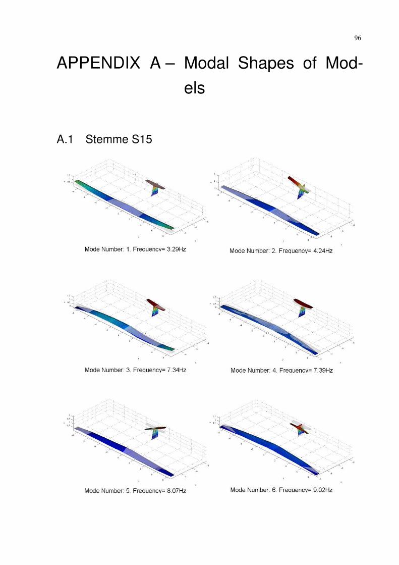
96
APPENDIX A – Modal Shapes of Mod-els
A.1 Stemme S15
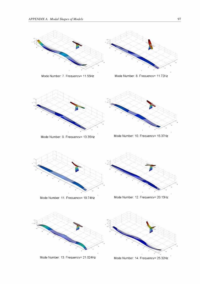
APPENDIX A. Modal Shapes of Models 97
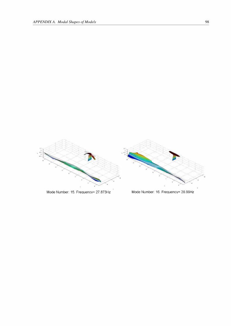
APPENDIX A. Modal Shapes of Models 98
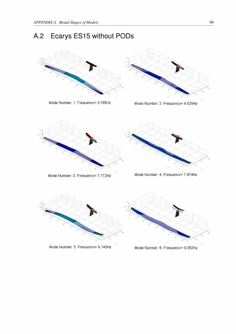
APPENDIX A. Modal Shapes of Models 99
A.2 Ecarys ES15 without PODs
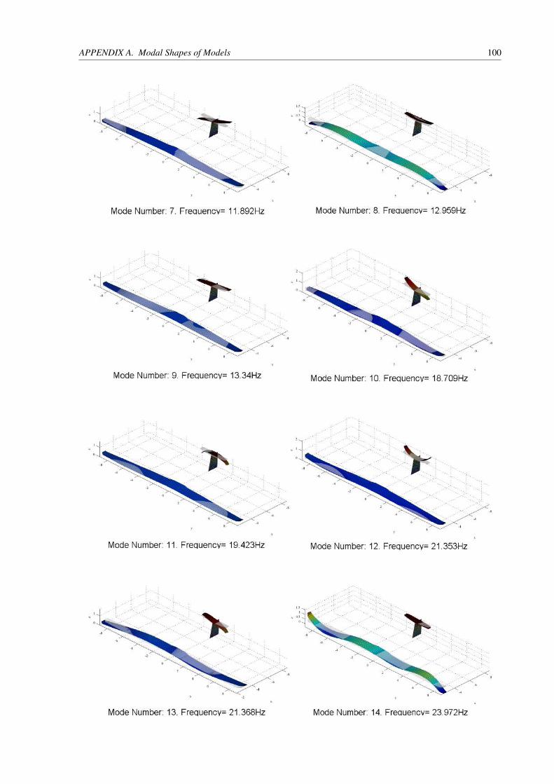
APPENDIX A. Modal Shapes of Models 100
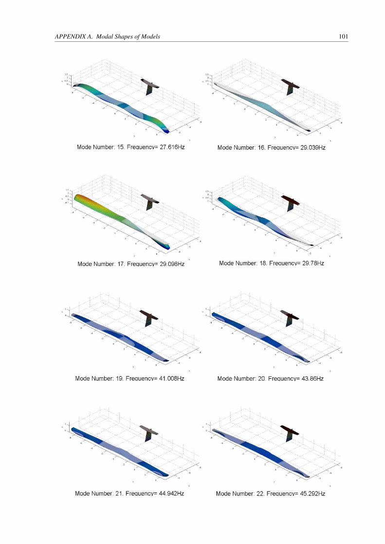
APPENDIX A. Modal Shapes of Models 101
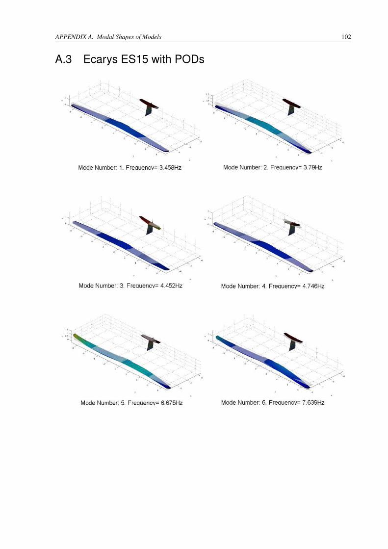
APPENDIX A. Modal Shapes of Models 102
A.3 Ecarys ES15 with PODs
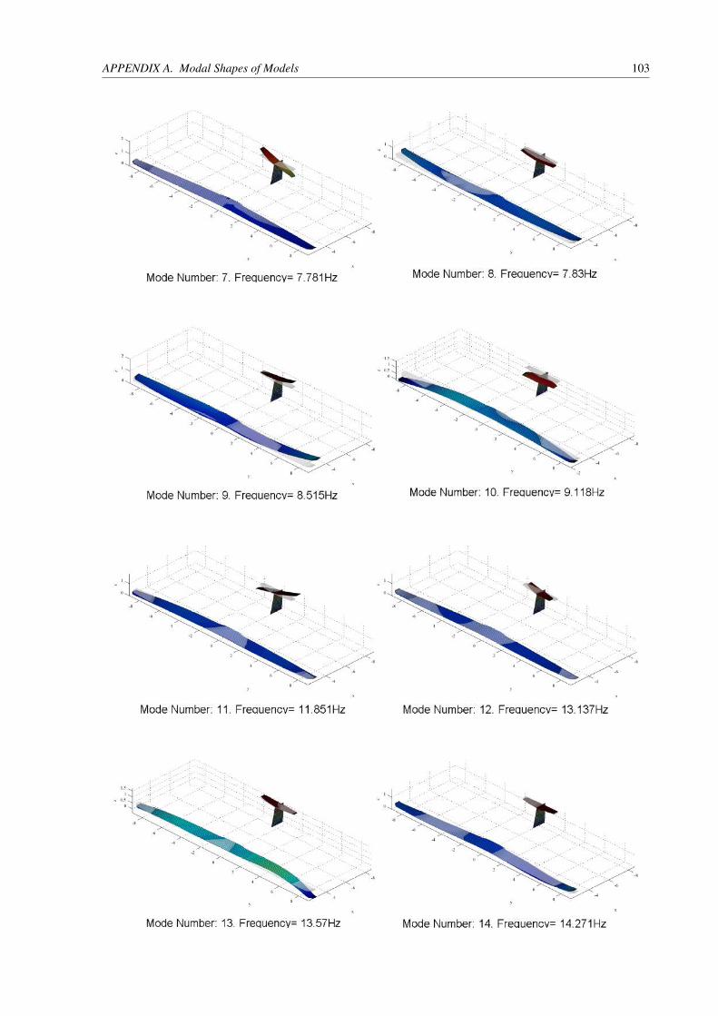
APPENDIX A. Modal Shapes of Models 103
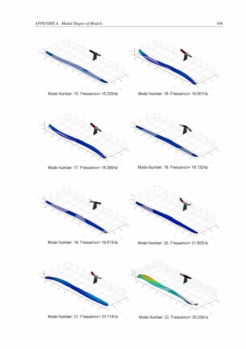
APPENDIX A. Modal Shapes of Models 104
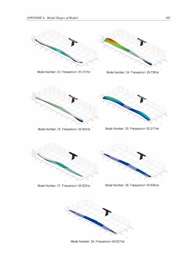
APPENDIX A. Modal Shapes of Models 105
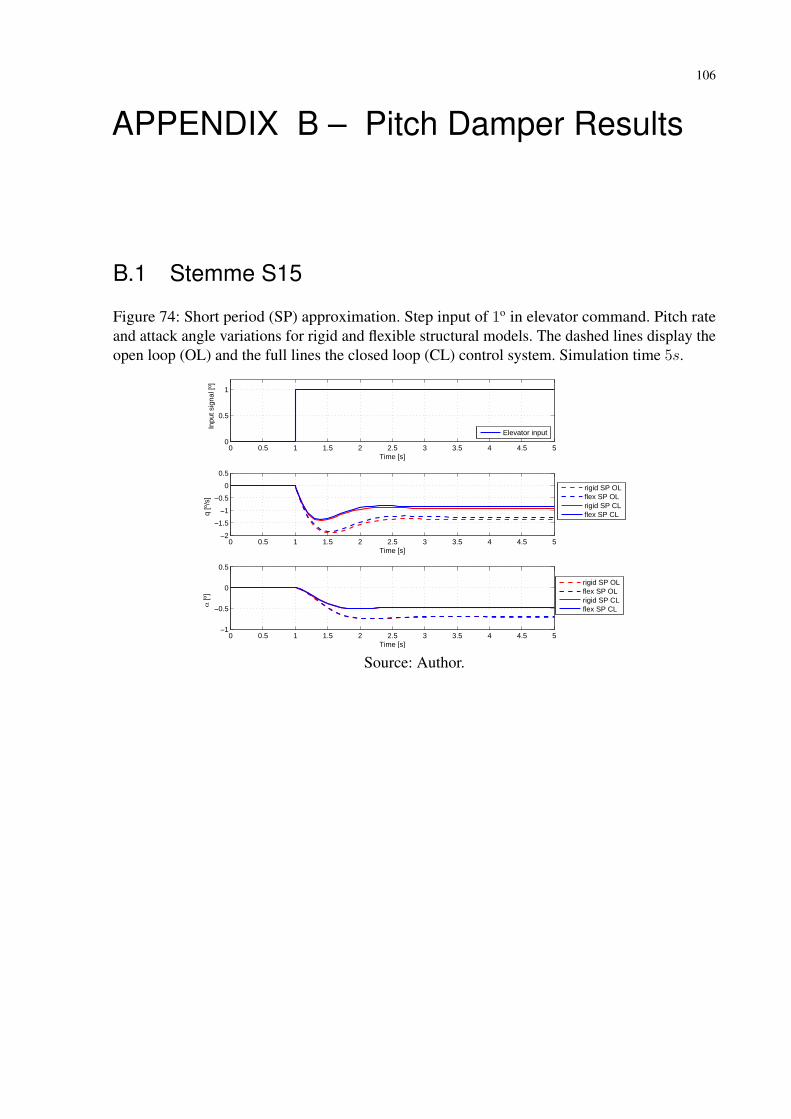
106
APPENDIX B – Pitch Damper Results
B.1 Stemme S15
Figure 74: Short period (SP) approximation. Step input of 1o in elevator command. Pitch rateand attack angle variations for rigid and flexible structural models. The dashed lines display theopen loop (OL) and the full lines the closed loop (CL) control system. Simulation time 5s.
0 0.5 1 1.5 2 2.5 3 3.5 4 4.5 50
0.5
1
Time [s]
Inpu
t sig
nal [
º]
Elevator input
0 0.5 1 1.5 2 2.5 3 3.5 4 4.5 5−2
−1.5
−1
−0.5
0
0.5
Time [s]
q [º
/s]
rigid SP OLflex SP OLrigid SP CLflex SP CL
0 0.5 1 1.5 2 2.5 3 3.5 4 4.5 5−1
−0.5
0
0.5
Time [s]
α[º
]
rigid SP OLflex SP OLrigid SP CLflex SP CL
Source: Author.
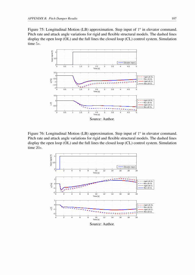
APPENDIX B. Pitch Damper Results 107
Figure 75: Longitudinal Motion (LB) approximation. Step input of 1o in elevator command.Pitch rate and attack angle variations for rigid and flexible structural models. The dashed linesdisplay the open loop (OL) and the full lines the closed loop (CL) control system. Simulationtime 5s.
0 0.5 1 1.5 2 2.5 3 3.5 4 4.5 50
0.5
1
Time [s]
Inpu
t sig
nal [
º]
Elevator input
0 0.5 1 1.5 2 2.5 3 3.5 4 4.5 5−2
−1.5
−1
−0.5
0
0.5
Time [s]
q [º
/s]
rigid LB OLflex LB OLrigid LB CLflex LB CL
0 0.5 1 1.5 2 2.5 3 3.5 4 4.5 5−1
−0.5
0
0.5
Time [s]
α[º
]
rigid LB OLflex LB OLrigid LB CLflex LB CL
Source: Author.
Figure 76: Longitudinal Motion (LB) approximation. Step input of 1o in elevator command.Pitch rate and attack angle variations for rigid and flexible structural models. The dashed linesdisplay the open loop (OL) and the full lines the closed loop (CL) control system. Simulationtime 20s.
0 2 4 6 8 10 12 14 16 18 200
0.5
1
Time [s]
Inpu
t sig
nal [
º]
Elevator input
0 2 4 6 8 10 12 14 16 18 20−2
−1
0
1
Time [s]
q [º
/s]
rigid LB OLflex LB OLrigid LB CLflex LB CL
0 2 4 6 8 10 12 14 16 18 20
−2
−1
0
1
Time [s]
α[º
]
rigid LB OLflex LB OLrigid LB CLflex LB CL
Source: Author.
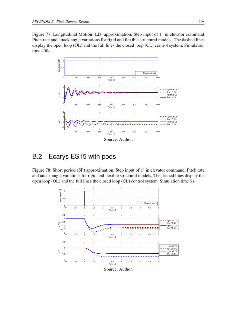
APPENDIX B. Pitch Damper Results 108
Figure 77: Longitudinal Motion (LB) approximation. Step input of 1o in elevator command.Pitch rate and attack angle variations for rigid and flexible structural models. The dashed linesdisplay the open loop (OL) and the full lines the closed loop (CL) control system. Simulationtime 400s.
0 50 100 150 200 250 300 350 4000
0.5
1
Time [s]
Inpu
t sig
nal [
º]
Elevator input
0 50 100 150 200 250 300 350 400−2
−1
0
1
Time [s]
q [º
/s]
rigid LB OLflex LB OLrigid LB CLflex LB CL
0 50 100 150 200 250 300 350 400
−2
−1
0
1
Time [s]
α[º
]
rigid LB OLflex LB OLrigid LB CLflex LB CL
Source: Author.
B.2 Ecarys ES15 with pods
Figure 78: Short period (SP) approximation. Step input of 1o in elevator command. Pitch rateand attack angle variations for rigid and flexible structural models. The dashed lines display theopen loop (OL) and the full lines the closed loop (CL) control system. Simulation time 5s.
0 0.5 1 1.5 2 2.5 3 3.5 4 4.5 50
0.5
1
Time [s]
Inpu
t sig
nal [
º]
Elevator input
0 0.5 1 1.5 2 2.5 3 3.5 4 4.5 5−2
−1.5
−1
−0.5
0
0.5
Time [s]
q [º
/s]
rigid SP OLflex SP OLrigid SP CLflex SP CL
0 0.5 1 1.5 2 2.5 3 3.5 4 4.5 5−1
−0.5
0
0.5
Time [s]
α[º
]
rigid SP OLflex SP OLrigid SP CLflex SP CL
Source: Author.
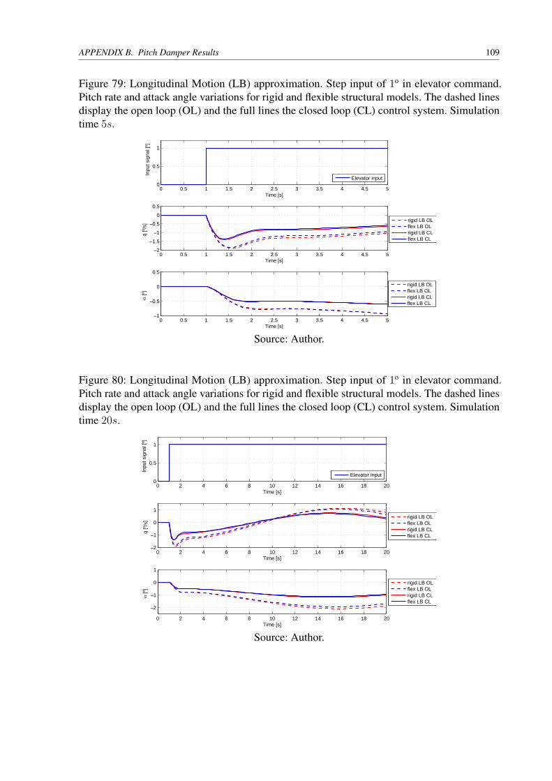
APPENDIX B. Pitch Damper Results 109
Figure 79: Longitudinal Motion (LB) approximation. Step input of 1o in elevator command.Pitch rate and attack angle variations for rigid and flexible structural models. The dashed linesdisplay the open loop (OL) and the full lines the closed loop (CL) control system. Simulationtime 5s.
0 0.5 1 1.5 2 2.5 3 3.5 4 4.5 50
0.5
1
Time [s]
Inpu
t sig
nal [
º]
Elevator input
0 0.5 1 1.5 2 2.5 3 3.5 4 4.5 5−2
−1.5
−1
−0.5
0
0.5
Time [s]
q [º
/s]
rigid LB OLflex LB OLrigid LB CLflex LB CL
0 0.5 1 1.5 2 2.5 3 3.5 4 4.5 5−1
−0.5
0
0.5
Time [s]
α[º
]
rigid LB OLflex LB OLrigid LB CLflex LB CL
Source: Author.
Figure 80: Longitudinal Motion (LB) approximation. Step input of 1o in elevator command.Pitch rate and attack angle variations for rigid and flexible structural models. The dashed linesdisplay the open loop (OL) and the full lines the closed loop (CL) control system. Simulationtime 20s.
0 2 4 6 8 10 12 14 16 18 200
0.5
1
Time [s]
Inpu
t sig
nal [
º]
Elevator input
0 2 4 6 8 10 12 14 16 18 20−2
−1
0
1
Time [s]
q [º
/s]
rigid LB OLflex LB OLrigid LB CLflex LB CL
0 2 4 6 8 10 12 14 16 18 20
−2
−1
0
1
Time [s]
α[º
]
rigid LB OLflex LB OLrigid LB CLflex LB CL
Source: Author.
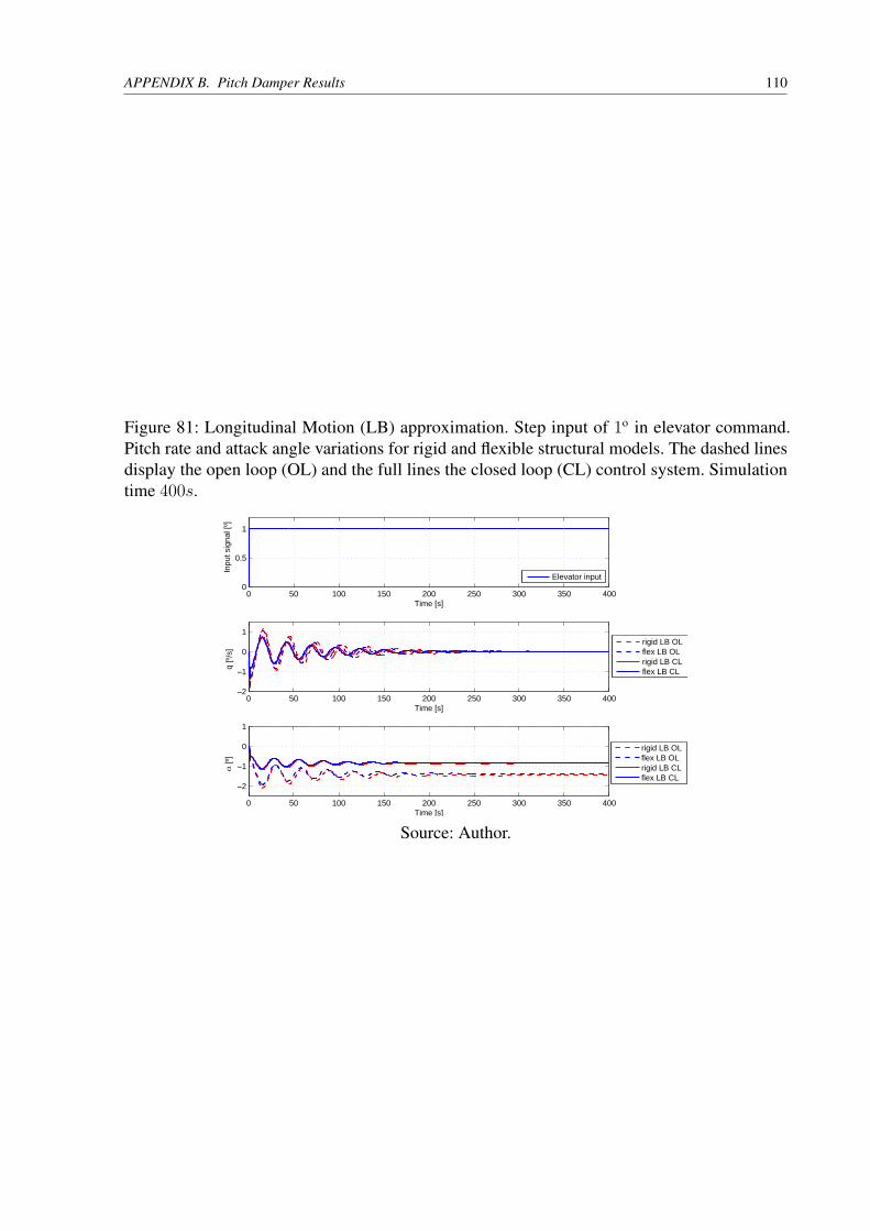
APPENDIX B. Pitch Damper Results 110
Figure 81: Longitudinal Motion (LB) approximation. Step input of 1o in elevator command.Pitch rate and attack angle variations for rigid and flexible structural models. The dashed linesdisplay the open loop (OL) and the full lines the closed loop (CL) control system. Simulationtime 400s.
0 50 100 150 200 250 300 350 4000
0.5
1
Time [s]
Inpu
t sig
nal [
º]
Elevator input
0 50 100 150 200 250 300 350 400−2
−1
0
1
Time [s]
q [º
/s]
rigid LB OLflex LB OLrigid LB CLflex LB CL
0 50 100 150 200 250 300 350 400
−2
−1
0
1
Time [s]
α[º
]
rigid LB OLflex LB OLrigid LB CLflex LB CL
Source: Author.
111
APPENDIX C – Implemented Algo-rithms
C.1 mfv2StructFlexSimInput.m
Listing C.1: mfv2StrucFlexSimInput.m
1 close all; clear all; clc;2 %% Choose the Configuration3 % PODs= 0; % without PODs4 PODs= 1; % with PODs5 WL=0; % without winglet6 % WL=1; % with winglet7 %% Import Data from Functions8 [GeoTemp,Streifen,GVTRefPoint]=InterpStreifenGVT(); %Geometry and Grids9 [Shapes,Modal_damp,Modal_freq,Modal_freq_Hz,Modal_names,Symmetry,Modal_mass,Geo]=
...10 ReadGVTData(PODs,GeoTemp,Streifen,GVTRefPoint,WL); % Shapes11 %% Define Inputs to FlexSim12 LocalEuler.wing = 0;13 LocalEuler.HE = 0;14 LocalEuler.VE = −90;15 LocalPos.wing = [0;0;0];16 LocalPos.HE = [0;0;0];17 LocalPos.VE = [0;0;0];18 R_coord_VE = [0;0;0];19 RefPoint = [0;0;0];20 RefStructPoint = [0;0;0];21 Scale = linspace(20,20,length(Shapes));22 Scale = Scale’;23 for count1=1:length(Shapes)24 Modal_names{count1,2} =char(64+count1);25 Modal_names{count1,3} =char(96+count1);26 end27 %% Save Structure File according to the configuration selected28 if PODs==0 && WL==029 % figname= ’150724_Structures_noPODs_noWL.mat’;30 figname= ’Structures_GVTVIInoPODSnoWL.mat’;31 save([’<input your directory>’,figname], ...

APPENDIX C. Implemented Algorithms 112
32 ’Geo’,’LocalEuler’,’LocalPos’,’Modal_damp’,’Modal_freq_Hz’,...33 ’Modal_freq’,’Modal_mass’,’R_coord_VE’,’RefPoint’,’Shapes’, ...34 ’Scale’,’RefStructPoint’,’Modal_names’,’Symmetry’); % ShapesGVT, GeoGVT35 disp([’Structure saved: configuration without PODs, "’,figname,’"’])36 elseif PODs==0 && WL==137 figname= ’Structures_GVTVIInoPODSWL.mat’;38 save([’<input your directory>’,figname], ...39 ’Geo’,’LocalEuler’,’LocalPos’,’Modal_damp’,’Modal_freq_Hz’, ...40 ’Modal_freq’,’Modal_mass’,’R_coord_VE’,’RefPoint’,’Shapes’, ...41 ’Scale’,’RefStructPoint’,’Modal_names’,’Symmetry’); % ShapesGVT, GeoGVT42 disp([’Structure saved: configuration without PODs, "’,figname,’"’])43 elseif PODs==1 && WL==044 figname= ’Structures_GVTVIIPODSnoWL.mat’;45 save([’<input your directory>’,figname], ...46 ’Geo’,’LocalEuler’,’LocalPos’,’Modal_damp’,’Modal_freq_Hz’, ...47 ’Modal_freq’,’Modal_mass’,’R_coord_VE’,’RefPoint’,’Shapes’, ...48 ’Scale’,’RefStructPoint’,’Modal_names’,’Symmetry’); % ShapesGVT, GeoGVT49 disp([’Structure saved: configuration without PODs, "’,figname,’"’])50 elseif PODs==1 && WL==151 figname= ’Structures_GVTVIIPODSWL.mat’;52 save([’<input your directory>’,figname], ...53 ’Geo’,’LocalEuler’,’LocalPos’,’Modal_damp’,’Modal_freq_Hz’, ...54 ’Modal_freq’,’Modal_mass’,’R_coord_VE’,’RefPoint’,’Shapes’, ...55 ’Scale’,’RefStructPoint’,’Modal_names’,’Symmetry’); % ShapesGVT, GeoGVT56 disp([’Structure saved: configuration without PODs, "’,figname,’"’])57 end
C.1.1 InterpStreifenGVT.m
Listing C.2: InterpStreifenGVT.m
1 function [GeoTemp,Streifen,GVTRefPoint]=InterpStreifenGVT()2 %% Load Data3 % Streifen Data aus GVT4 Streifen.wing = xlsread(’GeoStreifenTest.xlsx’,1); Streifen.wing(:,3:end)=
Streifen.wing(:,3:end)/100;5 Streifen.HE = xlsread(’GeoStreifenTest.xlsx’,2); Streifen.HE(:,3:end)=
Streifen.HE(:,3:end)/100;6 Streifen.VE = xlsread(’GeoStreifenTest.xlsx’,3); Streifen.VE(:,3:end)=
Streifen.VE(:,3:end)/100;7 Streifen.WL = xlsread(’GeoStreifenTest.xlsx’,4); Streifen.WL(:,3:end)=
Streifen.WL(:,3:end)/100;
APPENDIX C. Implemented Algorithms 113
8 % Geometry aus FEM: ’Structures_S6T_FEM.mat’9 load ’Geo.mat’
10 %% Feinheit der Streifen11 WingFeinheit = 5;12 WLFeinheit = WingFeinheit;13 HEFeinheit = WingFeinheit;14 VEFeinheit = WingFeinheit;15 %16 %% Fluegel17 % Vorderkante und Hinterkante Vektoren18 Vorderkante = max(Geo(1,1).wing); Vorderkante= Vorderkante(1,81:end); Vorderkante=
[−2.3650 Vorderkante −2.7710];19 Hinterkante = min(Geo(1,1).wing); Hinterkante= Hinterkante(1,81:end); Hinterkante=
[−3.5093 Hinterkante −2.9160];20 YKoord = Geo(1,2).wing(1,:); YKoord = YKoord(1,81:end); YKoord = [ 0 YKoord 8.9940];21 i=length(Vorderkante); ZKoord(1:i) = −0.3160; % Z Dimension is defined in the file/drawn
"Geometrie_S6_20110120_03.pdf"22
23 % Streifen: fuer den Fluegel sind 6524 % Streifen.wing(:,3) = Grenze25 % Streifen.wing(:,4) = Abschnittsbreite26 % Streifen.wing(:,5) = Abschinittsmitte27 % Streifen.wing(:,6) = halbe Flaechentiefe28 YKoordStreifen = Streifen.wing(33:end,5)’;29 VorderkanteStreifen = interp1(YKoord,Vorderkante,YKoordStreifen);30 ZKoordStreifen = interp1(YKoord,ZKoord,YKoordStreifen);31
32 %%%%%%%%%%%%%%%%%%%%33 % halbe Flaechentiefe= c34 %%%%%%%%%%%%%%%%%%%%35 for count1=1:length(VorderkanteStreifen)36 HinterkanteStreifen(count1) = −2∗Streifen.wing(32+count1,6)’ +
VorderkanteStreifen(count1);37 halbeFlachenTiefe(count1) = −1∗Streifen.wing(32+count1,6)’ +
VorderkanteStreifen(count1);38 end39
40 for count1=1:length(YKoordStreifen)41 TiefeStreifen = ...42 linspace(VorderkanteStreifen(count1),HinterkanteStreifen(count1), ...43 length(YKoordStreifen));44 TffStreifen(count1,:) = ...

APPENDIX C. Implemented Algorithms 114
45 linspace(TiefeStreifen(1),TiefeStreifen(end),WingFeinheit);46 end47
48 Geo_grid(1,1).wing1 = [flipdim(TffStreifen’,2) TffStreifen’]; % x values49 Geo_grid(1,2).wing1=zeros(WingFeinheit,length(Geo_grid(1,1).wing1)); % pre−alocate50 Geo_grid(1,3).wing1=zeros(WingFeinheit,length(Geo_grid(1,1).wing1)); % pre−alocate51
52 for count1=1:WingFeinheit53 Geo_grid(1,2).wing1(count1,:) = [flipdim(−YKoordStreifen,2) YKoordStreifen]; % y values54 Geo_grid(1,3).wing1(count1,:) = [flipdim(ZKoordStreifen,2) ZKoordStreifen]; % z values55 end56
57 %%%%%%58 %GRIDs59 %%%%%%60 YKoordGrid = Streifen.wing(33:end,3)’; % Grid benutzt YKoord von der Grenze61 ygrid = linspace(min(YKoordGrid),max(YKoordGrid),80);62 xvor = interp1(YKoordGrid,VorderkanteStreifen,ygrid);63 xhin = interp1(YKoordGrid,HinterkanteStreifen,ygrid); %HinterkanteStreifen264 zgrid = interp1(YKoordGrid,ZKoordStreifen,ygrid);65
66 for count1=1:length(ygrid)67 tiefe = linspace(xvor(count1),xhin(count1),length(ygrid));68 tff(count1,:) = linspace(tiefe(1),tiefe(end),15);69 end70
71 % Organize in structures with all wing’s geometrical data72 Grid(1,1).wing = [flipdim(tff’,2) tff’]; % x values73 Grid(1,2).wing=zeros(15,length(Grid(1,1).wing)); % pre−alocate74 Grid(1,3).wing=zeros(15,length(Grid(1,1).wing)); % pre−alocate75
76 for count1=1:1577 Grid(1,2).wing(count1,:) = [flipdim(−ygrid,2) ygrid]; % y values78 Grid(1,3).wing(count1,:) = [flipdim(zgrid,2) zgrid]; % z values79 end80
81
82 %% Wing let(s)83 % Vorderkante und Hinterkante Vektoren84 VorderkanteWL = −1∗[2.562 2.807 3.047];85 HinterkanteWL = −1∗[2.949 3.147 3.293];86

APPENDIX C. Implemented Algorithms 115
87 ZKoordWL = [8.994 8.994 8.994]; % in y Richtung88 YKoordWL = −1∗[0.3160 0.5325 0.749]; % in z Richtung89
90 % Streifen: fuer den Fluegel sind 6591 % Streifen.wing(:,3) = Grenze92 % Streifen.wing(:,4) = Abschnittsbreite93 % Streifen.wing(:,5) = Abschinittsmitte94 % Streifen.wing(:,6) = halbe Flaechentiefe95 YKoordStreifenWL = Streifen.WL(:,5)’; YKoordStreifenWL = −1∗(YKoordStreifenWL+0.316);96 VorderkanteStreifenWL = interp1(YKoordWL,VorderkanteWL,YKoordStreifenWL);97 HinterkanteStreifen2WL = interp1(YKoordWL,HinterkanteWL,YKoordStreifenWL);98 ZKoordStreifenWL = interp1(YKoordWL,ZKoordWL,YKoordStreifenWL);99
100 % Save Geometry101 for count1=1:length(YKoordStreifenWL)102 TiefeStreifenWL = ...103 linspace(VorderkanteStreifenWL(count1),HinterkanteStreifen2WL(count1), ...104 length(YKoordStreifenWL));105 TffStreifenWL(count1,:) = ...106 linspace(TiefeStreifenWL(1),TiefeStreifenWL(end),WLFeinheit);107 end108
109 Geo_grid(1,1).WL1 = [flipdim(TffStreifenWL’,2) TffStreifenWL’]; % x values110 for count1=1:WLFeinheit111 % y values (that in fact are z)112 Geo_grid(1,2).WL1(count1,:) = [flipdim(−YKoordStreifenWL,2) −YKoordStreifenWL];113 % z values (that in fact are y)114 Geo_grid(1,3).WL1(count1,:) = [flipdim(ZKoordStreifenWL,2) −ZKoordStreifenWL];115 end116
117 %%%%%%118 %GRIDs119 %%%%%%120 YKoordGrid = Streifen.WL(:,3)’; YKoordGrid = −1∗(YKoordGrid+0.316); % Grid benutzt
YKoord von der Grenze121 ygrid = linspace(max(YKoordGrid),min(YKoordGrid),20);122 xvor = interp1(YKoordGrid,VorderkanteStreifenWL,ygrid);123 xhin = interp1(YKoordGrid,HinterkanteStreifen2WL,ygrid); %HinterkanteStreifen2124 zgrid = interp1(YKoordGrid,ZKoordStreifenWL,ygrid);125
126 clear ’tiefe’; clear ’tff’;127 for count1=1:length(ygrid)
APPENDIX C. Implemented Algorithms 116
128 tiefe = linspace(xvor(count1),xhin(count1),length(ygrid));129 tff(count1,:) = linspace(tiefe(1),tiefe(end),15);130 end131
132 % Organize in structures with all wing’s geometrical data133 Grid(1,1).WL = [flipdim(tff’,2) tff’]; % x values134 Grid(1,2).WL =zeros(15,length(Grid(1,1).WL)); % pre−alocate135 Grid(1,3).WL =zeros(15,length(Grid(1,1).WL)); % pre−alocate136
137 for count1=1:15138 Grid(1,2).WL(count1,:) = [flipdim(−ygrid,2) −ygrid]; % y values139 Grid(1,3).WL(count1,:) = [flipdim(zgrid,2) −zgrid]; % z values140 end141
142 %% Hoehenleitwerk143
144 % Vorderkante und Hinterkante Vektoren145 VorderkanteHE = max(Geo(1,1).HE); VorderkanteHE= VorderkanteHE(1,41:end);
VorderkanteHE= ...146 [−7.6990 VorderkanteHE −7.932]; % −7.923 ist ein extrapolierten Punkt147 HinterkanteHE = min(Geo(1,1).HE); HinterkanteHE= HinterkanteHE(1,41:end);
HinterkanteHE= ...148 [−8.3290 HinterkanteHE −8.2562];149 YKoordHE = Geo(1,2).HE(1,:); YKoordHE = [ 0 YKoordHE(1,41:end) 1.6231];150 i=length(YKoordHE); ZKoordHE(1:i)= −1.564; % The value of z coordinate is151 %the same for horizontal empennage. Following the project drawings the value of 1.564 is
defined.152
153 % Streifen fuer das Hoehenleitwerk sind 17154 % Streifen.HE(:,3) = Grenze155 % Streifen.HE(:,4) = Abschnittsbreite156 % Streifen.HE(:,5) = Abschinittsmitte157 % Streifen.HE(:,6) = halbe Flaechentiefe158 YKoordStreifenHE = Streifen.HE(9:end,3)’;159 VorderkanteStreifenHE = interp1(YKoordHE,VorderkanteHE,YKoordStreifenHE);160 ZKoordStreifenHE = interp1(YKoordHE,ZKoordHE,YKoordStreifenHE);161
162 %%%%%%%%%%%%%%%%%%%%163 % halbe Fl?chentiefe= c164 %%%%%%%%%%%%%%%%%%%%165 for count1=1:length(VorderkanteStreifenHE)

APPENDIX C. Implemented Algorithms 117
166 HinterkanteStreifenHE(count1)= −2∗Streifen.HE(8+count1,6)’ +VorderkanteStreifenHE(count1);
167 halbeFlachenTiefeHE(count1) = −Streifen.HE(8+count1,6)’ +VorderkanteStreifenHE(count1);
168 % Differenz zwischen Hinterkante durch Interpolation oder mit der halbe Flaechentiefe169 % diffHE(count1)= (HinterkanteStreifen2HE(count1)/HinterkanteStreifenHE(count1)−1)∗100;
% Werte in Prozent170 end171
172 for count1=1:length(YKoordStreifenHE)173 TiefeStreifenHE = ...174 linspace(VorderkanteStreifenHE(count1),HinterkanteStreifenHE(count1), ...175 length(YKoordStreifenHE));176 TffStreifenHE(count1,:) = ...177 linspace(TiefeStreifenHE(1),TiefeStreifenHE(end),HEFeinheit);178 end179
180 Geo_grid(1,1).HE1 = [flipdim(TffStreifenHE’,2) TffStreifenHE’]; % x values181 Geo_grid(1,2).HE1=zeros(HEFeinheit,length(Geo_grid(1,1).HE1)); % pre−alocate182 Geo_grid(1,3).HE1=zeros(HEFeinheit,length(Geo_grid(1,1).HE1)); % pre−alocate183 for count1=1:HEFeinheit184 Geo_grid(1,2).HE1(count1,:) = [flipdim(−YKoordStreifenHE,2) YKoordStreifenHE]; % y
values185 Geo_grid(1,3).HE1(count1,:) = [flipdim(ZKoordStreifenHE,2) ZKoordStreifenHE]; % z
values186 end187
188 %%%%%%189 %GRIDs190 %%%%%%191 YKoordGrid = Streifen.HE(9:end,3)’; % Grid benutzt YKoord von der Grenze192 ygridHE = linspace(min(YKoordGrid),max(YKoordGrid),40);193 xvorHE = interp1(YKoordGrid,VorderkanteStreifenHE,ygridHE);194 xhinHE = interp1(YKoordGrid,HinterkanteStreifenHE,ygridHE); % HinterkanteStreifen2HE195 zgridHE = interp1(YKoordGrid,ZKoordStreifenHE,ygridHE);196
197 clear ’tiefe’; clear ’tff’;198 for count1=1:length(ygridHE)199 tiefe = linspace(xvorHE(count1),xhinHE(count1),length(ygridHE));200 tff(count1,:) = linspace(tiefe(1),tiefe(end),15);201 end202
APPENDIX C. Implemented Algorithms 118
203 % Organize in structures with all HE’s geometrical data204 Grid(1,1).HE = [flipdim(tff’,2) tff’]; % x values205 Grid(1,2).HE=zeros(15,length(Grid(1,1).HE)); % pre−alocate206 Grid(1,3).HE=zeros(15,length(Grid(1,1).HE)); % pre−alocate207
208 for count1=1:15209 Grid(1,2).HE(count1,:) = [flipdim(−ygridHE,2) ygridHE]; % y values210 Grid(1,3).HE(count1,:) = [flipdim(zgridHE,2) zgridHE]; % z values211 end212
213 %% Seitenleitwerk214
215 % Vorderkante und Hinterkante Vektoren216 VorderkanteVE = max(Geo(1,1).VE); % in x Richtung217 HinterkanteVE = min(Geo(1,1).VE); % in x Richtung218
219 YKoordVE = Geo(1,2).VE(1,:); % in z Richtung220 i= length(YKoordVE); ZKoordVE(1:i) = 0; % in y Richtung221
222 % Streifen: fuer den Fluegel sind 65223 % Streifen.wing(:,3) = Grenze224 % Streifen.wing(:,4) = Abschnittsbreite225 % Streifen.wing(:,5) = Abschinittsmitte226 % Streifen.wing(:,6) = halbe Flaechentiefe227 YKoordStreifenVE = Streifen.VE(:,5)’;228 VorderkanteStreifenVE = interp1(YKoordVE,VorderkanteVE,YKoordStreifenVE);229 ZKoordStreifenVE = interp1(YKoordVE,ZKoordVE,YKoordStreifenVE);230
231 %%%%%%%%%%%%%%%%%%%%232 % halbe Flaechentiefe= c233 %%%%%%%%%%%%%%%%%%%%234 for count1=1:length(VorderkanteStreifenVE)235 HinterkanteStreifenVE(count1)= −2∗Streifen.VE(count1,6)’ +
VorderkanteStreifenVE(count1);236 halbeFlachenTiefeVE(count1) = −Streifen.VE(count1,6)’ +
VorderkanteStreifenVE(count1);237 % Differenz zwischen Hinterkante durch Interpolation oder mit der halbe Flaechentiefe238 % diffHE(count1)= (HinterkanteStreifen2HE(count1)/HinterkanteStreifenHE(count1)−1)∗100;
% Werte in Prozent239 end240
241 for count1=1:length(YKoordStreifenVE)
APPENDIX C. Implemented Algorithms 119
242 TiefeStreifenVE = ...243 linspace(VorderkanteStreifenVE(count1),HinterkanteStreifenVE(count1), ...244 length(YKoordStreifenVE));245 TffStreifenVE(count1,:) = ...246 linspace(TiefeStreifenVE(1),TiefeStreifenVE(end),VEFeinheit);247 end248
249 Geo_grid(1,1).VE1 = [TffStreifenVE’]; % x values250 for count1=1:VEFeinheit251 Geo_grid(1,2).VE1(count1,:) = YKoordStreifenVE; % y values (that in fact are z)252 Geo_grid(1,3).VE1(count1,:) = ZKoordStreifenVE; % z values (that in fact are y)253 end254
255 %%%%%%%256 % GRIDs257 %%%%%%%258 YKoordGrid = Streifen.VE(:,3)’; % Grid benutzt YKoord von der Grenze259 ygridVE = linspace(min(YKoordGrid),max(YKoordGrid),80);260 xvorVE = interp1(YKoordGrid,VorderkanteStreifenVE,ygridVE);261 xhinVE = interp1(YKoordGrid,HinterkanteStreifenVE,ygridVE); % HinterkanteStreifen2VE262 zgridVE = interp1(YKoordGrid,ZKoordStreifenVE,ygridVE);263
264 clear ’tiefe’; clear ’tff’;265 for count1=1:length(ygridVE)266 tiefe = linspace(xvorVE(count1),xhinVE(count1),length(ygridVE));267 tff(count1,:) = linspace(tiefe(1),tiefe(end),15);268 end269
270 % Organize in structures with all VE’s geometrical data271 Grid(1,1).VE = tff’; % x values272 Grid(1,2).VE=zeros(15,length(Grid(1,1).VE)); % pre−alocate273 Grid(1,3).VE=zeros(15,length(Grid(1,1).VE)); % pre−alocate274
275 for count1=1:15276 Grid(1,2).VE(count1,:) = ygridVE; % y values277 Grid(1,3).VE(count1,:) = zgridVE; % z values278 end279
280 %% Elastische Achse: EA 1/4∗chord from leading edge point281 % wing282 for count1=1:length(VorderkanteStreifen) % Werte abspeichern
APPENDIX C. Implemented Algorithms 120
283 GVTRefPoint(1,1).wing(count1,:)= VorderkanteStreifen(count1) −(1/2)∗Streifen.wing(32+count1,6)’;
284 GVTRefPoint(1,2).wing(count1,:)= YKoordStreifen(count1);285 end286 GVTRefPoint(1,3).wing = ZKoordStreifen;287 %%% Ganze Fluegel organizieren288 GVTRefPoint(1,1).wing= [flipdim(GVTRefPoint(1,1).wing’,2)
GVTRefPoint(1,1).wing(2:end,1)’]; % x values289 GVTRefPoint(1,2).wing= [flipdim(−GVTRefPoint(1,2).wing’,2)
GVTRefPoint(1,2).wing(2:end,1)’]; % y values290 GVTRefPoint(1,3).wing= [GVTRefPoint(1,3).wing GVTRefPoint(1,3).wing(1,2:end) ]; % z
values291
292 % Hoehenleitwerk293 for count1=1:length(VorderkanteStreifenHE) % Werte abspeichern294 GVTRefPoint(1,1).HE(count1,:)= VorderkanteStreifenHE(count1) −
(1/2)∗Streifen.HE(8+count1,6)’;295 GVTRefPoint(1,2).HE(count1,:)= YKoordStreifenHE(count1);296 end297 GVTRefPoint(1,3).HE = ZKoordStreifenHE;298 %%% Ganze Hoehenleitwerk organizieren299 GVTRefPoint(1,1).HE= [flipdim(GVTRefPoint(1,1).HE’,2) GVTRefPoint(1,1).HE(2:end,1)’]; %
x values300 GVTRefPoint(1,2).HE= [flipdim(−GVTRefPoint(1,2).HE’,2) GVTRefPoint(1,2).HE(2:end,1)’];
% y values301 GVTRefPoint(1,3).HE= [GVTRefPoint(1,3).HE GVTRefPoint(1,3).HE(1,2:end) ]; % z values302
303 % WingLet304 for count1=1:length(VorderkanteStreifenWL) % Werte abspeichern305 GVTRefPoint(1,1).WL(count1,:)= VorderkanteStreifenWL(count1) −
(1/2)∗Streifen.WL(count1,6)’;306 GVTRefPoint(1,2).WL(count1,:)= YKoordStreifenWL(count1);307 end308 GVTRefPoint(1,3).WL = ZKoordStreifenWL;309 %%% Ganze WingLet organizieren310 GVTRefPoint(1,1).WL= [flipdim(GVTRefPoint(1,1).WL’,2) GVTRefPoint(1,1).WL’]; % x values311 GVTRefPoint(1,2).WL= [flipdim(GVTRefPoint(1,2).WL’,2) GVTRefPoint(1,2).WL’]; % z values312 GVTRefPoint(1,3).WL= [GVTRefPoint(1,3).WL GVTRefPoint(1,3).WL]; % y values313
314 % Seitenleitwerk315 for count1=1:length(VorderkanteStreifenVE) % Werte abspeichern

APPENDIX C. Implemented Algorithms 121
316 GVTRefPoint(1,1).VE(count1,:)= VorderkanteStreifenVE(count1) −(1/2)∗Streifen.VE(count1,6)’;
317 GVTRefPoint(1,2).VE(count1,:)= YKoordStreifenVE(count1);318 end319 GVTRefPoint(1,1).VE=GVTRefPoint(1,1).VE’; GVTRefPoint(1,2).VE=GVTRefPoint(1,2).VE;320 GVTRefPoint(1,3).VE = ZKoordStreifenVE;321
322 %% Output Definitions323 %!!!!!!!!!!!!!!!!!!!!!!!!!!!!!!!!!!!!!!!!!!!!!!!!!!!!!!!!!!!!!!!!!!!!!!!!!324 % Based on the comparison done with this routine the following consideration will be adopted:325 %!!!!326 % The geometry data that will be used to define the leading edge values is327 % based on the middle point of every strip defined by the experimental328 % procedure, GVT. It means that the x coordinates of the leading edge are equal329 % the value of the trailing edge plus two times c.330 %!!!!!!!!!!!!!!!!!!!!!!!!!!!!!!!!!!!!!!!!!!!!!!!!!!!!!!!!!!!!!!!!!!!!!!!!!331
332 % STREIFEN333 % wing334 Streifen(1,1).wing = Geo_grid(1,1).wing1; Streifen(1,1).wing(:,33)=[];335 Streifen(1,2).wing = Geo_grid(1,2).wing1; Streifen(1,2).wing(:,33)=[];336 Streifen(1,3).wing = Geo_grid(1,3).wing1; Streifen(1,3).wing(:,33)=[];337 % wing lets338 Streifen(1,1).WL = Geo_grid(1,1).WL1;339 Streifen(1,2).WL = −Geo_grid(1,2).WL1;340 Streifen(1,3).WL = Geo_grid(1,3).WL1;341 % right342 Streifen(1,1).WL = flipdim(Geo_grid(1,1).WL1,2);343 Streifen(1,2).WL = flipdim(−Geo_grid(1,2).WL1,2);344 Streifen(1,3).WL = flipdim(Geo_grid(1,3).WL1,2);345 % Horizontal empennage346 Streifen(1,1).HE = Geo_grid(1,1).HE1; Streifen(1,1).HE(:,9) = [];347 Streifen(1,2).HE = Geo_grid(1,2).HE1; Streifen(1,2).HE(:,9) = [];348 Streifen(1,3).HE = Geo_grid(1,3).HE1; Streifen(1,3).HE(:,9) = [];349 % Vertical empennage350 Streifen(1,1).VE = Geo_grid(1,1).VE1;351 Streifen(1,2).VE = −Geo_grid(1,2).VE1;352 Streifen(1,3).VE = Geo_grid(1,3).VE1;353
354 % GEOMETRY Geo in form of GRIDs355 % wing356 GeoTemp(1,1).wing = Grid(1,1).wing;
APPENDIX C. Implemented Algorithms 122
357 GeoTemp(1,2).wing = Grid(1,2).wing;358 GeoTemp(1,3).wing = Grid(1,3).wing;359 % wing lets360 % left361 GeoTemp(1,1).WL = Grid(1,1).WL;362 GeoTemp(1,2).WL = −1∗Grid(1,2).WL;363 GeoTemp(1,3).WL = −1∗Grid(1,3).WL;364 % right365 GeoTemp(1,1).WL(:,1:length(Grid(1,1).WL)/2) = Grid(1,1).WL(:,1:length(Grid(1,1).WL)/2);366 GeoTemp(1,2).WL(:,1:length(Grid(1,1).WL)/2) = −Grid(1,2).WL(:,1:length(Grid(1,1).WL)/2);367 GeoTemp(1,3).WL(:,1:length(Grid(1,1).WL)/2) =
−1∗flipdim(Grid(1,3).WL(:,1:length(Grid(1,1).WL)/2),2);368 % Horizontal empennage369 GeoTemp(1,1).HE = Grid(1,1).HE;370 GeoTemp(1,2).HE = Grid(1,2).HE;371 GeoTemp(1,3).HE = Grid(1,3).HE;372 % Vertical empennage373 GeoTemp(1,1).VE = Grid(1,1).VE;374 GeoTemp(1,2).VE = −Grid(1,2).VE;375 GeoTemp(1,3).VE = Grid(1,3).VE;376
377 % % Correction Winglet: add a tiny displacement in z coordinates because if378 % % wing let and wing have 90deg between each other the interpolation in379 % % STRIPS DEFINITION doesn’t work380 dywl=0.01;%m381 for count1=1:20382 GeoTemp(1,3).WL(:,20+count1) = GeoTemp(1,3).WL(:,20+count1)+(dywl/100)∗count1;383 end384 GeoTemp(1,3).WL(:,1:20) = −flipdim(GeoTemp(1,3).WL(:,21:end),2);385 end
C.1.2 ReadGVTData.m
Listing C.3: ReadGVTData.m
1 function[Shapes,Modal_damp,Modal_freq,Modal_freq_Hz,Modal_names,Symmetry,Modal_mass,Geo]=...
2 ReadGVTData(PODs,GeoTemp,Streifen,GVTRefPoint,WL)3 if PODs==14 % with PODs5 cd(’<input your directory>’);
APPENDIX C. Implemented Algorithms 123
6 elseif PODs==07 % without PODs8 cd(’<input your directory>’);9 end
10 %% Read the GVT Data11 Names= dir; Names= Names(3:end);12 for count1=1:length(Names)13 FileName(count1,:)= {Names(count1).name};14 end15 FileName= cell2mat(FileName);16
17 Data= [];18 for count1=1:length(FileName)19 fileToRead1= FileName(count1,:);20
21 DELIMITER = ’ ’;22 HEADERLINES = 103;23
24 % Import the file25 rawData1 = importdata(fileToRead1, DELIMITER, HEADERLINES);26
27 [~,name] = fileparts(fileToRead1);28 newData1.(genvarname(name)) = rawData1;29
30 % Create new variables in the base workspace from those fields.31 vars = fieldnames(newData1);32 for i = 1:length(vars)33 assignin(’base’, vars{i}, newData1.(vars{i}));34 end35
36 Data= [Data newData1.(vars{i})];37 end38 %% Sort out GVT Data39 % Data= Data(6:end−1,:); % save only the displacements and rotations. With characteres
the function cell2mat doesn’t work40 % Data= cell2mat(Data); % converts to mat variable41 for count1=1:length(FileName)42 Modes(count1,1).name = Data{2,count1}(1:6);43 Modes(count1,1).GenMass = str2num(Data{2,count1}(10:19));44 Modes(count1,1).Freq = str2num(Data{2,count1}(30:38));45 Modes(count1,1).Damping = str2num(Data{2,count1}(20:29));46 i=0;
APPENDIX C. Implemented Algorithms 124
47 for count2=6:(length(Data)−1) % The first 6 lines have the mode names, frequency andgen. mass.
48 i=i+1;49 Modes(count1,1).Data(i,1) = str2num(Data{count2,count1}(1:2));50 Modes(count1,1).Data(i,2) = str2num(Data{count2,count1}(4:5));51 Modes(count1,1).Data(i,3) = str2num(Data{count2,count1}(11:18));52 Modes(count1,1).Data(i,4) = str2num(Data{count2,count1}(21:28));53 Modes(count1,1).Data(i,5) = str2num(Data{count2,count1}(31:38));54 Modes(count1,1).Data(i,6) = str2num(Data{count2,count1}(41:48));55 end56 end57 % Sort values based on the frequency58 Frequency = [Modes.Freq]; % create a vector with Frequency59 [Value,Pos] = unique(Frequency); % sort the values and their position60 Frequency = Value’; % Frequency vector61 Modal_freq_Hz = Frequency; % Flexsim input name62 Modal_freq = Modal_freq_Hz∗2∗pi;63 Modal_damp = [Modes.Damping]’; % Modal damping64 Modes(:,1) = Modes(Pos,1); % Sort the structure: Modes65 FileName = FileName(Pos,:);66 Modal_names = cellstr(FileName); % Variable Modal_names67
68 for count1=1:length(FileName)69 Modal_mass(count1,:) = Modes(count1).GenMass∗1e−4; % Generalized Mass∗1e−4:
cm^2 to m^270 % Wing71 ShapesStreifen1(count1,1).wing= Modes(count1,1).Data(1:65,3);% plunging72 ShapesStreifen1(count1,2).wing= Modes(count1,1).Data(1:65,4);% pitching73 ShapesStreifen1(count1,3).wing= Modes(count1,1).Data(1:65,5);% −−−74 ShapesStreifen1(count1,4).wing= Modes(count1,1).Data(1:65,6);% lagging75 ShapesStreifen1(count1,5).wing= Modes(count1,1).name; % mode name76 % Horizontal empennage77 ShapesStreifen1(count1,1).HE = Modes(count1,1).Data(66:82,3);78 ShapesStreifen1(count1,2).HE = Modes(count1,1).Data(66:82,4);79 ShapesStreifen1(count1,3).HE = Modes(count1,1).Data(66:82,5);80 ShapesStreifen1(count1,4).HE = Modes(count1,1).Data(66:82,6);81 ShapesStreifen1(count1,5).HE= Modes(count1,1).name;82 % Vertical empennage83 ShapesStreifen1(count1,1).VE = Modes(count1,1).Data(83:91,3);84 ShapesStreifen1(count1,2).VE = Modes(count1,1).Data(83:91,4);85 ShapesStreifen1(count1,3).VE = Modes(count1,1).Data(83:91,5);86 ShapesStreifen1(count1,4).VE = Modes(count1,1).Data(83:91,6);

APPENDIX C. Implemented Algorithms 125
87 ShapesStreifen1(count1,5).VE= Modes(count1,1).name;88 % Wing let: 92 until 94 Winglet right and 95 until 97 wing let left89 % Corrections in Position90 ShapesStreifen1(count1,1).WL(1:3,:) =−flipdim(Modes(count1,1).Data(95:97,3),1); % left91 ShapesStreifen1(count1,1).WL(4:6,:) =−flipdim(Modes(count1,1).Data(92:94,3),1); %
right92
93 ShapesStreifen1(count1,2).WL(1:3,:) = flipdim(Modes(count1,1).Data(95:97,4),1);94 ShapesStreifen1(count1,2).WL(4:6,:) = flipdim(Modes(count1,1).Data(92:94,4),1);95
96 ShapesStreifen1(count1,3).WL(1:3,:) = flipdim(Modes(count1,1).Data(95:97,5),1);97 ShapesStreifen1(count1,3).WL(4:6,:) = flipdim(Modes(count1,1).Data(92:94,5),1);98
99 ShapesStreifen1(count1,4).WL(1:3,:) = flipdim(Modes(count1,1).Data(95:97,6),1);100 ShapesStreifen1(count1,4).WL(4:6,:) = flipdim(Modes(count1,1).Data(92:94,6),1);101 end102 %103 %% DIMENSIONS: DISPLACEMENTS/VERSCHIEBUNG104 % FaktConvert= 0.001; % mm to m105 FaktConvert= 0.01; % cm to m106 % FaktConvert= 0.1; % dc to m107 for ne=1:length(FileName)108 ShapesStreifen1(ne,1).wing=FaktConvert∗ShapesStreifen1(ne,1).wing;109 ShapesStreifen1(ne,4).wing=FaktConvert∗ShapesStreifen1(ne,4).wing;110 % PITCHING ANGLE THETA:111 % ShapesStreifen1(ne,2).wing=0.1∗ShapesStreifen1(ne,2).wing;112 %113 ShapesStreifen1(ne,1).HE=FaktConvert∗ShapesStreifen1(ne,1).HE;114 ShapesStreifen1(ne,4).HE=FaktConvert∗ShapesStreifen1(ne,4).HE;115 % PITCHING ANGLE THETA:116 % ShapesStreifen1(ne,2).HE=0.1∗ShapesStreifen1(ne,2).HE;117 %118 ShapesStreifen1(ne,1).VE=FaktConvert∗ShapesStreifen1(ne,1).VE;119 ShapesStreifen1(ne,4).VE=FaktConvert∗ShapesStreifen1(ne,4).VE;120 % PITCHING ANGLE THETA:121 % ShapesStreifen1(ne,2).VE=0.1∗ShapesStreifen1(ne,2).VE;122 %123 ShapesStreifen1(ne,1).WL=FaktConvert∗ShapesStreifen1(ne,1).WL;124 ShapesStreifen1(ne,4).WL=FaktConvert∗ShapesStreifen1(ne,4).WL;125 % PITCHING ANGLE THETA:126 % ShapesStreifen1(ne,2).WL=0.1∗ShapesStreifen1(ne,2).WL;127 end
APPENDIX C. Implemented Algorithms 126
128 %% 2. INTERPOLATION (DREIECK) − DISPLACEMENTS FROM THE POINT TO THESTRIP LINE
129 %%% Inputs %%%130 % StreifenPunkt = Floating Point throught the Strip;131 % Theta angle − Verdreheung = ShapesStreifen1(1,2).XXX132 % Measured point = GVTRefPoint.XXX133 % dx_EA,dy_EA,dz_EA = ShapesStreifen1(1,1).XXX, ShapesStreifen1(1,2).XXX,
ShapesStreifen1(1,3).XXX134 % ShapesStreifen1(~,1).XXXX = PLUNGING135 % ShapesStreifen1(~,2).XXXX = PITCHING136 % ShapesStreifen1(~,3).XXXX = NO VALUES137 % ShapesStreifen1(~,4).XXXX = LAGGING138 [lineStreifenWing,~] = size(Streifen(1,1).wing);139 for modeNum=1:length(ShapesStreifen1) % mode number140 for stripNum=1:length(GVTRefPoint(1,1).wing) % strip number141 % Wing142 for pointNum=1:lineStreifenWing % Points through the chord at each strip143 % SCALENE TRIANGLE144 % [SILVESTRE,2012 − Methodology..., Page 57] "Observe that just145 % the modal shape?s component perpendicular to the lifting surface,146 % thus the only component considered in the incremental aerodynamic model, is
displayed."147 StreifenPunkt= Streifen(1,1).wing(pointNum,stripNum);148 % HIPOTENUSA. side of triangle = length of the elastic axe in x direction149 c= StreifenPunkt−GVTRefPoint(1,1).wing(1,stripNum);150 % displacement in z direction = height of the scalene triangle.151 dzp1d = c∗sin(ShapesStreifen1(modeNum,2).wing(stripNum,1));152 %153 % Allocate the displacements at each strip point for each modal form154 ShapesStreifen2(modeNum,1).wing(pointNum,stripNum)= ...155 ShapesStreifen1(modeNum,4).wing(stripNum,1); %+ dxp1d; % point
displacement + gvt displacement156 ShapesStreifen2(modeNum,2).wing(pointNum,stripNum)= ...157 0; % there’s no displacement in y direction158 ShapesStreifen2(modeNum,3).wing(pointNum,stripNum)= ...159 ShapesStreifen1(modeNum,1).wing(stripNum,1) + dzp1d; % point
displacement + gvt displacement160 end161 end162 % HE163 [lineStreifenHE,~] = size(Streifen(1,1).HE);164 for stripNum=1:length(GVTRefPoint(1,1).HE) % number of strips
APPENDIX C. Implemented Algorithms 127
165 for pointNum=1:lineStreifenHE;166 % SCALENE TRIANGLE167 StreifenPunkt= Streifen(1,1).HE(pointNum,stripNum);168 % side of triangle = length of the elastic axe in x direction169 c= StreifenPunkt−GVTRefPoint(1,1).HE(1,stripNum);170 % displacement in z direction = height of the scalene triangle.171 dzp1d = c∗sin(ShapesStreifen1(modeNum,2).HE(stripNum,1));172 % dxp1d = dzp1d∗tan(ShapesStreifen1(modeNum,2).HE(stripNum,1)); % displacement in x
direction173 % saving the displacements at each strip point for each modal form174 ShapesStreifen2(modeNum,1).HE(pointNum,stripNum)= ...175 ShapesStreifen1(modeNum,4).HE(stripNum,1);% + dxp1d; % point
displacement + gvt displacement176 ShapesStreifen2(modeNum,2).HE(pointNum,stripNum)= ...177 0; % there’s no displacement in y direction178 ShapesStreifen2(modeNum,3).HE(pointNum,stripNum)= ...179 ShapesStreifen1(modeNum,1).HE(stripNum,1) + dzp1d; % point
displacement + gvt displacement180 end181 end182 % WL183 [lineStreifenWL,~] = size(Streifen(1,1).WL);184 for stripNum=1:length(GVTRefPoint(1,1).WL) % number of strips185 for pointNum=1:lineStreifenWL186 % SCALENE TRIANGLE187 StreifenPunkt= Streifen(1,1).WL(pointNum,stripNum);188 % side of triangle = length of the elastic axe in x direction189 c= StreifenPunkt−GVTRefPoint(1,1).WL(1,stripNum);190 % displacement in z direction = height of the scalene triangle.191 dzp1d = c∗sin(ShapesStreifen1(modeNum,2).WL(stripNum,1));192 % dxp1d = dzp1d∗tan(ShapesStreifen1(modeNum,2).WL(stripNum,1)); % displacement in x
direction193 % saving the displacements at each strip point for each modal form194 ShapesStreifen2(modeNum,1).WL(pointNum,stripNum)= ...195 ShapesStreifen1(modeNum,4).WL(stripNum,1); %+ dxp1d; % point
displacement + gvt displacement196 ShapesStreifen2(modeNum,2).WL(pointNum,stripNum)= ...197 0; % there’s no displacement in y direction198 ShapesStreifen2(modeNum,3).WL(pointNum,stripNum)= ...199 ShapesStreifen1(modeNum,1).WL(stripNum,1) + dzp1d; % point
displacement + gvt displacement200 end
APPENDIX C. Implemented Algorithms 128
201 end202 % VE203 [lineStreifenVE,~] = size(Streifen(1,1).VE);204 for stripNum=1:length(GVTRefPoint(1,1).VE) % number of strips205 for pointNum=1:lineStreifenVE206 % SCALENE TRIANGLE207 StreifenPunkt= Streifen(1,1).VE(pointNum,stripNum);208 % side of triangle = length of the elastic axe in x direction209 c= StreifenPunkt−GVTRefPoint(1,1).VE(1,stripNum);210 % displacement in z direction = height of the scalene triangle.211 dzp1d = c∗sin(ShapesStreifen1(modeNum,2).VE(stripNum,1));212 ShapesStreifen2(modeNum,1).VE(pointNum,stripNum)=
ShapesStreifen1(modeNum,4).VE(stripNum,1);% + dxp1d; % pointdisplacement + gvt displacement
213 ShapesStreifen2(modeNum,2).VE(pointNum,stripNum)= 0; % there’s nodisplacement in y direction
214 ShapesStreifen2(modeNum,3).VE(pointNum,stripNum)=ShapesStreifen1(modeNum,1).VE(stripNum,1) + dzp1d; % pointdisplacement + gvt displacement
215 end216 end217
218 % % Correction in WL Displacements219 ShapesStreifen2(modeNum,3).WL(:,1:3)= ShapesStreifen2(modeNum,3).WL(:,1:3);220 ShapesStreifen2(modeNum,3).WL(:,4:6)=
flipdim(ShapesStreifen2(modeNum,3).WL(:,4:6),2);221 end222 %% PLOT RESULTS INTERPOLATION 2223 % ABC=1;224 % % faktor=20;225 % % for m=1:6 % mode number226 % % Geometry227 % surf(Streifen(1,1).wing, Streifen(1,2).wing, −Streifen(1,3).wing); hold on;228 % surf(Streifen(1,1).HE, Streifen(1,2).HE, −Streifen(1,3).HE);229 % surf(Streifen(1,1).VE, Streifen(1,3).VE, −Streifen(1,2).VE); alpha(0.0);230 % % Modes231 % surf(Streifen(1,1).wing + faktor∗ShapesStreifen2(m,1).wing, ...232 % Streifen(1,2).wing, − Streifen(1,3).wing + faktor∗ShapesStreifen2(m,3).wing); hold on233 % surf(Streifen(1,1).HE + faktor∗ShapesStreifen2(m,1).HE, ...234 % Streifen(1,2).HE, − Streifen(1,3).HE + faktor∗ShapesStreifen2(m,3).HE);235 % %236 % surf(Streifen(1,1).VE + faktor∗ShapesStreifen2(m,1).VE, ...
APPENDIX C. Implemented Algorithms 129
237 % Streifen(1,3).VE + faktor∗ShapesStreifen2(m,3).VE, −Streifen(1,2).VE);238 % axis equal; grid on;239 % xlabel ’x’;ylabel ’y’;zlabel ’z’; view(130,30);240 % % end241 %% 3. INTERPOLATION (GRIDDATA)242 % Interpolations Function243 % F.dxgrid = griddata(F.x , F.y , F.dx , F.xgrid , F.ygrid ,’v4’)244 % F.x, F.y and F.z must have the same size245 %%%%% DATA246 % F.x = Streifen(1,1).XXX % F.y = Streifen(1,2).XXX247 % F.xgrid = Geo(1,1).XXX % F.ygrid = Geo(1,2).XXX248 % F.dx = ShapesStreifen2(1,X).XXX249 for modeNum=1:length(FileName)250 % wing251 ShapesTemp(modeNum,1).wing = griddata(Streifen(1,1).wing, Streifen(1,2).wing,
ShapesStreifen2(modeNum,1).wing, GeoTemp(:,1).wing, GeoTemp(:,2).wing,’v4’); %x and y
252 ShapesTemp(modeNum,2).wing = griddata(Streifen(1,1).wing, Streifen(1,2).wing,ShapesStreifen2(modeNum,2).wing, GeoTemp(:,1).wing, GeoTemp(:,2).wing,’v4’); %y and z
253 ShapesTemp(modeNum,3).wing = griddata(Streifen(1,1).wing, Streifen(1,2).wing,ShapesStreifen2(modeNum,3).wing, GeoTemp(:,1).wing, GeoTemp(:,2).wing,’v4’); %z and y
254 % HE255 ShapesTemp(modeNum,1).HE = griddata(Streifen(1,1).HE, Streifen(1,2).HE,
ShapesStreifen2(modeNum,1).HE, GeoTemp(:,1).HE, GeoTemp(:,2).HE,’v4’); % xand y
256 ShapesTemp(modeNum,2).HE = griddata(Streifen(1,1).HE, Streifen(1,2).HE,ShapesStreifen2(modeNum,2).HE, GeoTemp(:,1).HE, GeoTemp(:,2).HE,’v4’); % yand z
257 ShapesTemp(modeNum,3).HE = griddata(Streifen(1,1).HE, Streifen(1,2).HE,ShapesStreifen2(modeNum,3).HE, GeoTemp(:,1).HE, GeoTemp(:,2).HE,’v4’); % zand y
258 % VE259 ShapesTemp(modeNum,1).VE = griddata(Streifen(1,1).VE, Streifen(1,2).VE,
ShapesStreifen2(modeNum,1).VE, GeoTemp(:,1).VE, GeoTemp(:,2).VE,’v4’); % xand y
260 ShapesTemp(modeNum,2).VE = griddata(Streifen(1,1).VE, Streifen(1,2).VE,ShapesStreifen2(modeNum,3).VE, GeoTemp(:,1).VE, GeoTemp(:,2).VE,’v4’); % yand z
261 ShapesTemp(modeNum,3).VE = griddata(Streifen(1,1).VE, Streifen(1,2).VE,ShapesStreifen2(modeNum,2).VE, GeoTemp(:,1).VE, GeoTemp(:,2).VE,’v4’); % z
APPENDIX C. Implemented Algorithms 130
and y262 % ShapesTemp(modeNum,1).VE = griddata(Streifen(1,1).VE, Streifen(1,2).VE,
ShapesStreifen2(modeNum,1).VE, GeoTemp(:,1).VE, GeoTemp(:,2).VE,’v4’); % x and y263 % ShapesTemp(modeNum,2).VE = griddata(Streifen(1,1).VE, Streifen(1,2).VE,
ShapesStreifen2(modeNum,2).VE, GeoTemp(:,1).VE, GeoTemp(:,2).VE,’v4’); % y and z264 % ShapesTemp(modeNum,3).VE = griddata(Streifen(1,1).VE, Streifen(1,2).VE,
ShapesStreifen2(modeNum,3).VE, GeoTemp(:,1).VE, GeoTemp(:,2).VE,’v4’); % z and y265
266 % Wing let right267 ShapesTemp(modeNum,1).WLr = griddata(Streifen(1,1).WL(:,1:3),
Streifen(1,2).WL(:,1:3), ShapesStreifen2(modeNum,1).WL(:,1:3),GeoTemp(:,1).WL(:,1:20), GeoTemp(:,2).WL(:,1:20),’v4’); % x and y
268 ShapesTemp(modeNum,2).WLr = griddata(Streifen(1,1).WL(:,1:3),Streifen(1,2).WL(:,1:3), ShapesStreifen2(modeNum,3).WL(:,1:3),GeoTemp(:,1).WL(:,1:20), GeoTemp(:,2).WL(:,1:20),’v4’); % y and z
269 ShapesTemp(modeNum,3).WLr = griddata(Streifen(1,1).WL(:,1:3),Streifen(1,2).WL(:,1:3), ShapesStreifen2(modeNum,2).WL(:,1:3),GeoTemp(:,1).WL(:,1:20), GeoTemp(:,2).WL(:,1:20),’v4’); % z and y
270 % wing let left % (:,3).WL = Fx,Fz,dz,Fxgrid,Fzgrid271 ShapesTemp(modeNum,1).WLl = griddata(Streifen(1,1).WL(:,4:6),
Streifen(1,2).WL(:,4:6), ShapesStreifen2(modeNum,1).WL(:,4:6),GeoTemp(:,1).WL(:,21:40), GeoTemp(:,2).WL(:,21:40),’v4’); % x and y
272 ShapesTemp(modeNum,2).WLl = griddata(Streifen(1,1).WL(:,4:6),Streifen(1,2).WL(:,4:6), ShapesStreifen2(modeNum,3).WL(:,4:6),GeoTemp(:,1).WL(:,21:40), GeoTemp(:,2).WL(:,21:40),’v4’); % y and z
273 ShapesTemp(modeNum,3).WLl = griddata(Streifen(1,1).WL(:,4:6),Streifen(1,2).WL(:,4:6), ShapesStreifen2(modeNum,2).WL(:,4:6),GeoTemp(:,1).WL(:,21:40), GeoTemp(:,2).WL(:,21:40),’v4’); % z and y
274
275 end276 %% Verbindung vom Fluegel und Wing Let277 if WL==1278 for count1=1:length(FileName) % number of modes279 % WingLet: Letzte Streifen rechts und erste Streifen links280 for count2=1:length(ShapesTemp(1,1).WLr)281 % x direction282 ShapesTemp(count1,1).WLr(:,count2) = ShapesTemp(count1,1).WLr(:,count2) +
ShapesTemp(count1,1).wing(:,1);283 ShapesTemp(count1,1).WLl(:,count2) = ShapesTemp(count1,1).WLl(:,count2) +
ShapesTemp(count1,1).wing(:,end);284 % z direction
APPENDIX C. Implemented Algorithms 131
285 ShapesTemp(count1,3).WLr(:,count2) = ShapesTemp(count1,3).WLr(:,count2) +ShapesTemp(count1,3).wing(:,1);
286 ShapesTemp(count1,3).WLl(:,count2) = ShapesTemp(count1,3).WLl(:,count2) +ShapesTemp(count1,3).wing(:,end);
287 end288 % y direction289 ShapesTemp(count1,2).wing(:,1) = ShapesTemp(count1,2).WLr(:,20) +
ShapesTemp(count1,2).wing(:,1);290 ShapesTemp(count1,2).wing(:,end) = ShapesTemp(count1,2).WLl(:, 1) +
ShapesTemp(count1,2).wing(:,end);291 % Corrections292 if PODs==0 && count1==4 % mode 4, configuration with PODs293 ShapesTemp(count1,2).wing(:,2)= ShapesTemp(count1,2).WLr(:,20) +
ShapesTemp(count1,2).wing(:,2);294 end295 end296 end297 %% Output Definitions298 % Variable Symmetry299 if PODs==0300 Symmetry= {’symmetric’; ’anti−symmetric’;’anti−symmetric’;’symmetric’; ...301 ’anti−symmetric’;’symmetric’;’anti−symmetric’;’symmetric’;...302 ’anti−symmetric’;’anti−symmetric’; ’symmetric’;’symmetric’; ...303 ’anti−symmetric’;’anti−symmetric’; ’symmetric’;’symmetric’;...304 ’anti−symmetric’;’symmetric’;’anti−symmetric’;’anti−symmetric’; ...305 ’symmetric’;’symmetric’};306 elseif PODs==1307 Symmetry= {’anty−symmetric’;’symmetric’;’anty−symmetric’;’anty−symmetric’; ...308 ’anty−symmetric’; ’anty−symmetric’;’anty−symmetric’;’symmetric’;...309 ’anty−symmetric’;’anty−symmetric’; ’anty−symmetric’;’anty−symmetric’; ...310 ’anty−symmetric’;’anty−symmetric’;’anty−symmetric’; ’anty−symmetric’; ...311 ’anty−symmetric’;’symmetric’;’anty−symmetric’;’symmetric’;’anty−symmetric’;...312 ’anty−symmetric’;’symmetric’;’anty−symmetric’;’symmetric’;’symmetric’; ...313 ’anty−symmetric’; ’anty−symmetric’;’symmetric’;};314 end315
316 if WL==1317 % Geo: saving wing and WL together318 Geo(1,1).wing= [GeoTemp(1,1).WL(:,1:20) GeoTemp(1,1).wing
GeoTemp(1,1).WL(:,21:end)]; Geo(1,1).wing(:,100)=[];319 Geo(1,2).wing= [GeoTemp(1,3).WL(:,1:20) GeoTemp(1,2).wing
GeoTemp(1,3).WL(:,21:end)]; Geo(1,2).wing(:,100)=[];
APPENDIX C. Implemented Algorithms 132
320 Geo(1,3).wing= [GeoTemp(1,2).WL(:,1:20) GeoTemp(1,3).wingGeoTemp(1,2).WL(:,21:end)]; Geo(1,3).wing(:,100)=[];
321 Geo(1,1).HE= GeoTemp(1,1).HE; Geo(1,1).HE(:,40)= [];322 Geo(1,2).HE= GeoTemp(1,2).HE; Geo(1,2).HE(:,40)= [];323 Geo(1,3).HE= GeoTemp(1,3).HE; Geo(1,3).HE(:,40)= [];324 Geo(1,1).VE= GeoTemp(1,1).VE;325 Geo(1,2).VE= −GeoTemp(1,2).VE;326 Geo(1,3).VE= GeoTemp(1,3).VE;327 elseif WL==0328 % without wing let329 Geo(1,1).wing= GeoTemp(1,1).wing; Geo(1,1).wing(:,80)=[];330 Geo(1,2).wing= GeoTemp(1,2).wing; Geo(1,2).wing(:,80)=[];331 Geo(1,3).wing= GeoTemp(1,3).wing; Geo(1,3).wing(:,80)=[];332 Geo(1,1).HE= GeoTemp(1,1).HE; Geo(1,1).HE(:,40)= [];333 Geo(1,2).HE= GeoTemp(1,2).HE; Geo(1,2).HE(:,40)= [];334 Geo(1,3).HE= GeoTemp(1,3).HE; Geo(1,3).HE(:,40)= [];335 Geo(1,1).VE= GeoTemp(1,1).VE;336 Geo(1,2).VE= −GeoTemp(1,2).VE;337 Geo(1,3).VE= GeoTemp(1,3).VE;338 end339 % Shapes: saving wing and WL together340 for count1=1:length(FileName)341 if WL==1342 Shapes(count1,1).wing= [ShapesTemp(count1,1).WLr ShapesTemp(count1,1).wing
ShapesTemp(count1,1).WLl];343 Shapes(count1,2).wing= [ShapesTemp(count1,2).WLr ShapesTemp(count1,2).wing
ShapesTemp(count1,2).WLl];344 Shapes(count1,3).wing= [ShapesTemp(count1,3).WLr ShapesTemp(count1,3).wing
ShapesTemp(count1,3).WLl];345 Shapes(count1,1).HE = ShapesTemp(count1,1).HE;346 Shapes(count1,2).HE = ShapesTemp(count1,2).HE;347 Shapes(count1,3).HE = ShapesTemp(count1,3).HE;348 Shapes(count1,1).VE = ShapesTemp(count1,1).VE;349 Shapes(count1,2).VE = ShapesTemp(count1,3).VE;350 Shapes(count1,3).VE = ShapesTemp(count1,2).VE;351 elseif WL==0352 % without winglet353 Shapes(count1,1).wing= ShapesTemp(count1,1).wing;354 Shapes(count1,2).wing= ShapesTemp(count1,2).wing;355 Shapes(count1,3).wing= ShapesTemp(count1,3).wing;356 Shapes(count1,1).HE = ShapesTemp(count1,1).HE;357 Shapes(count1,2).HE = ShapesTemp(count1,2).HE;
APPENDIX C. Implemented Algorithms 133
358 Shapes(count1,3).HE = ShapesTemp(count1,3).HE;359 Shapes(count1,1).VE = ShapesTemp(count1,1).VE;360 Shapes(count1,2).VE = ShapesTemp(count1,3).VE;361 Shapes(count1,3).VE = ShapesTemp(count1,2).VE;362 end363 % corrections in doubled strips364 Shapes(count1,1).wing(:,100)= [];365 Shapes(count1,2).wing(:,100)= [];366 Shapes(count1,3).wing(:,100)= [];367 Shapes(count1,1).HE(:,40) = [];368 Shapes(count1,2).HE(:,40) = [];369 Shapes(count1,3).HE(:,40) = [];370 end371 end
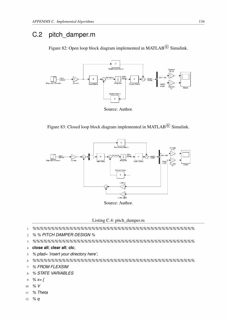
APPENDIX C. Implemented Algorithms 134
C.2 pitch_damper.m
Figure 82: Open loop block diagram implemented in MATLAB R© Simulink.
Source: Author.
Figure 83: Closed loop block diagram implemented in MATLAB R© Simulink.
Source: Author.
Listing C.4: pitch_damper.m
1 %%%%%%%%%%%%%%%%%%%%%%%%%%%%%%%%%%%%%%%%%%%%2 % % PITCH DAMPER DESIGN %3 %%%%%%%%%%%%%%%%%%%%%%%%%%%%%%%%%%%%%%%%%%%%4 close all; clear all; clc;5 % pfad= ’insert your directory here’;6 %%%%%%%%%%%%%%%%%%%%%%%%%%%%%%%%%%%%%%%%%%%%7 % FROM FLEXSIM8 % STATE VARIABLES9 % x= [
10 % V11 % Theta12 % q
APPENDIX C. Implemented Algorithms 135
13 % alpha14 % H15 % beta16 % p17 % phi18 % r19 % ]20 %21 % Control Variables22 % u = [23 % Shub = eta_F24 % Querruder = xi25 % Fluegelklappen = eta_k26 % Hoehenruder = eta27 % Seitenruder = zeta28 % ]29 %%%%%%%%%%%%%%%%%%%%%%%%%%%%%%%%%%%%%%%%%%%%30 % % MODELS %31 %%%%%%%%%%%%%%%%%%%%%%%%%%%%%%%%%%%%%%%%%%%%32 % Model=1; % model 1 = LCSv833 % Model=2; % model 2 = ohne PODs korrigiert34 % Model=3; % model 3 = ohne PODs35 % Model=4; % model 4 = mit PODs korrigiert36 Model=5; % model 5 = mit PODs37 %%%%%%%%%%%%%%%%%%%%%%%%%%%%%%%%%%%%%%%%%%%%38 if Model==1 % LCSv8 elev 1deg39 state_space_name_rigid = ’State_space_rigid_lcsv8_elev1deg.mat’; % rigid40 state_space_name_flex = ’State_space_flex_lcsv8_elev1deg.mat’; % flex41 disp([’Model Nr.: ’, Model])42 disp([’Modelo rigido: ’,state_space_name_rigid])43 disp([’Modelo elastico: ’,state_space_name_flex])44 elseif Model==2 % ECARY ES15 ohne PODs korrigiert45 state_space_name_rigid = ’State_space_rigid_noPODsnoWL_elev1deg_corriged.mat’;
% rigid46 state_space_name_flex = ’State_space_flex_noPODsnoWL_elev1deg_corriged.mat’; %
flex47 disp([’Model Nr.: ’,Model])48 disp([’Modelo rigido: ’,state_space_name_rigid])49 disp([’Modelo elastico: ’,state_space_name_flex])50 elseif Model==3 % ECARY ES15 ohne PODs51 state_space_name_rigid = ’State_space_rigid_noPODsnoWL_elev1deg.mat’; % rigid52 state_space_name_flex = ’State_space_flex_noPODsnoWL_elev1deg.mat’; % flex

APPENDIX C. Implemented Algorithms 136
53 disp([’Model Nr.: ’,Model])54 disp([’Modelo rigido: ’,state_space_name_rigid])55 disp([’Modelo elastico: ’,state_space_name_flex])56 %elseif Model==457 % state_space_name_rigid = ’State_space_rigid_noPODsnoWL_elev1deg.mat’; % rigid58 % state_space_name_flex = ’State_space_flex_noPODsnoWL_elev1deg.mat’; % flex59 % disp([’Model Nr.: ’,Model])60 % disp([’Modelo rigido: ’,state_space_name_rigid])61 % disp([’Modelo elastico: ’,state_space_name_flex])62 elseif Model==563 state_space_name_rigid = ’State_space_rigid_PODsnoWL_elev1deg.mat’; % rigid64 state_space_name_flex = ’State_space_flex_PODsnoWL_elev1deg.mat’; % flex65 disp([’Model Nr.: ’,Model])66 disp([’Modelo rigido: ’,state_space_name_rigid])67 disp([’Modelo elastico: ’,state_space_name_flex])68 end69 %%%%%%%%%%%%%%%%%%%%%%%%%%%%%%%%%%%%%%%%%%%%70 %% LOAD SYSTEM MATRICES71 %%%%%%%%%%%%%%%%%%%%%%%%%%%%%%%%%%%%%%%%%%%%72 % Load System Matrices73 %state_space_name = ’State_space_rigid_lcsv8_elev1deg’; % rigid74 load([pfad,state_space_name_rigid])75 %76 % System Matrix A77 temp= Lin_Model(1,1);78 A= cell2mat(temp);79 % System Matrix B80 temp= Lin_Model(1,2);81 B= cell2mat(temp);82 % System Matrix C83 C=eye(length(A));84 % System Matrix D85 [m,n]= size(B);86 D=zeros(m,n);87 %% FULL RIGIB BODY (RB) AIRCRAFT88 % State−space system89 SS_rigid=ss(A,B,C,D);90 % pzmap91 f11=figure();92 pzmap(SS_rigid); legend ’FULL RIGIB BODY (RB) AIRCRAFT’; grid on;93 % System Characteristics94 [wn_RB,D_RB,poles_RB]=damp(SS_rigid);

APPENDIX C. Implemented Algorithms 137
95 %% RB LONGITUDINAL MOTION APPROXIMATION (LB)96 A_LB(1,:)= A(1,1:4); % Geschwindigkeit97 A_LB(2,:)= A(2,1:4); % Theta98 A_LB(3,:)= A(3,1:4); % q99 A_LB(4,:)= A(4,1:4); % alpha
100 %101 B_LB(1:4,1)= B(1:4,1); % Shub102 B_LB(1:4,2)= B(1:4,4); % Hoehenruder103 %104 C_LB= eye(4,4);105 D_LB= zeros(4,2);106 % State Space Model107 SS_LB_rigid = ss(A_LB,B_LB,C_LB,D_LB);108 % Transfer Function109 TF_LB_rigid = tf(SS_LB_rigid);110 % TFs: Input 1= eta_f111 % Input 2= eta112 %113 % Output1= q114 % Output2= a = Alpha115 % Output3= V116 % Output4= t = theta117 % eta118 F_q_eta = TF_LB_rigid(3,2);119 F_a_eta = TF_LB_rigid(4,2);120 F_V_eta = TF_LB_rigid(1,2);121 F_t_eta = TF_LB_rigid(2,2);122 %123 % Characteristische Polynom ableiten124 Charpol_LB = poly(A_LB);125 % Pollstellen: 1 und 2= Phugoid (PH) (V und Theta)126 % 3 und 4= Anstelwinkelschwingung (AS) (q und Alpha)127 pole_LB = roots(Charpol_LB);128 % PN−Diagramm129 f2=figure();130 pzmap(SS_LB_rigid); grid on; legend(’ RB Longitudinal Motion Aproximation’)131 %132 % Natural Frequency and Damping133 % [Wn,zeta] = damp(sys). Wn = vector with natural frequencies134 % Zeta = vector with damping ratios135 [wn_RB_LB,D_RB_LB,P_LB_RB] = damp(SS_LB_rigid);136 nfFreqAS = wn_RB_LB(3);

APPENDIX C. Implemented Algorithms 138
137 dampAS = D_RB_LB(3);138 %139 %%%%%%%%%%%%%%%%%%%%%%%%%%%%%%%%%%%%%%%%%%%%140 %% SHORT PERIOD APPROXIMATION %141 %%%%%%%%%%%%%%%%%%%%%%%%%%%%%%%%%%%%%%%%%%%%142 A_LB_AS(1,1:2)= A_LB(3,3:4);143 A_LB_AS(2,1:2)= A_LB(4,3:4);144 B_LB_AS = B_LB(3:4,2);145 C_LB_AS = eye(size(A_LB_AS));146 D_LB_AS = zeros(size(B_LB_AS));147 % State−space148 SS_LB_AS_Rigid = ss(A_LB_AS,B_LB_AS,C_LB_AS,D_LB_AS);149 % Transfer Functions150 TF_LB_AS_Rigid = tf(SS_LB_AS_Rigid);151 % eta x q152 F_q_eta_AS_rigid = TF_LB_AS_Rigid(1);153 F_alpha_AS_rigid = TF_LB_AS_Rigid(2);154 % step(F_q_eta,’b’,F_q_eta_AS_rigid,’r’); % compare the Short period155 % approximation156 %%%%%%%%%%%%%%%%%%%%%%%%%%%%%%%%%%%%%%%%%%%%157 %% STEUERBARKEIT %158 %%%%%%%%%%%%%%%%%%%%%%%%%%%%%%%%%%%%%%%%%%%%159 %160 Q_S = [B_LB_AS, A_LB_AS∗B_LB_AS];161 Steuerbarkeit = det(Q_S); % Ist ungleich Null, deswegen ist das System Steuerbar162 % Regelungsnormalform163 rnf_LB_AS = canon(SS_LB_AS_Rigid,’companion’);164 %165 %%%%%%%%%%%%%%%%%%%%%%%%%%%%%%%%%%%%%%%%%%%%166 %% POLE PLACEMENT − SHORT PERIOD APPROXIMATION %167 %%%%%%%%%%%%%%%%%%%%%%%%%%%%%%%%%%%%%%%%%%%%168 % Desired damping and frequency169 w0_AS_ziel = 2.500; % rad/s170 D_AS_ziel = 0.707; % Find the reference171 % Roots of a 2nd order system with the desired damping and frequency values172 p_AS = roots([1 2∗D_AS_ziel∗w0_AS_ziel w0_AS_ziel^2]);173 % Pole placement174 kT = place(A_LB_AS,B_LB_AS,p_AS);175 % K−values176 k_eta_q = kT(1);177 k_eta_alpha = kT(2);178 %
APPENDIX C. Implemented Algorithms 139
179 %%%%%%%%%%%%%%%%%%%%%%%%%%%%%%%%%%%%%%%%%%%%180 %% MODIFIED RB SHORT PERIOD APPROXIMATION (CLOSED LOOP)181 %%%%%%%%%%%%%%%%%%%%%%%%%%%%%%%%%%%%%%%%%%%%182 K_LB_AS_Rigid = zeros(size(B_LB_AS))’;183 K_LB_AS_Rigid(1) = −kT(1);184 K_LB_AS_Rigid(2) = −kT(2);185 % Modified System Matrices186 A_LB_AS_mod = A_LB_AS−B_LB_AS∗K_LB_AS_Rigid;187 B_LB_AS_mod = B_LB_AS;188 C_LB_AS_mod = C_LB_AS;189 D_LB_AS_mod = D_LB_AS;190 % State Space of modified system191 SS_LB_AS_rigid_mod = ss(A_LB_AS_mod,B_LB_AS_mod,C_LB_AS_mod,D_LB_AS_mod);192 % Transfer Function193 TF_LB_AS_rigid_mod = tf(SS_LB_AS_rigid_mod);194 %195 F_q_eta_AS_rigid_mod = TF_LB_AS_rigid_mod(1);196 F_alpha_eta_AS_rigid_mod = TF_LB_AS_rigid_mod(2);197 % step(F_q_eta,’b’,F_q_eta_AS_rigid,’r’,F_q_eta_AS_rigid_mod,’m’); % compare the Short
period198 %%%%%%%%%%%%%%%%%%%%%%%%%%%%%%%%%%%%%%%%%%%%199 %% MODIFIED RB LONGITUDINAL APPROXIMATION (CLOSED LOOP)200 %%%%%%%%%%%%%%%%%%%%%%%%%%%%%%%%%%%%%%%%%%%%201 K_LB_Rigid = zeros(size(B_LB))’;202 K_LB_Rigid(2,3) = −kT(1); %kT(1); %−kT(1); %203 K_LB_Rigid(2,4) = −kT(2); %?kT(2); %−kT(2); %204 % Modified System Matrices205 A_LB_mod = A_LB−B_LB∗K_LB_Rigid;206 B_LB_mod = B_LB;207 C_LB_mod = C_LB;208 D_LB_mod = D_LB;209 % State Space of modified system210 SS_LB_rigid_mod = ss(A_LB_mod,B_LB_mod,C_LB_mod,D_LB_mod);211 % Transfer Function212 TF_LB_rigid_mod = tf(SS_LB_rigid_mod);213 %214 F_q_eta_rigid_LB_mod = TF_LB_rigid_mod(3,2);215 F_alpha_eta_rigid_LB_mod = TF_LB_rigid_mod(4,2);216 % step(F_q_eta,’b’,F_q_eta_AS_rigid,’r’,F_q_eta_rigid_LB_mod,’m’); % compare the Short
period217 %%%%%%%%%%%%%%%%%%%%%%%%%%%%%%%%%%%%%%%%%%%%218 %% MODIFIED FULL RIGIB BODY (RB) AIRCRAFT
APPENDIX C. Implemented Algorithms 140
219 %%%%%%%%%%%%%%%%%%%%%%%%%%%%%%%%%%%%%%%%%%%%220 K_Rigid = zeros(size(B))’;221 K_Rigid(4,3) = −kT(1);222 K_Rigid(4,4) = −kT(2);223 % Modified System Matrices224 A_Rigid_mod = A−B∗K_Rigid;225 B_Rigid_mod = B;226 C_Rigid_mod = C;227 D_Rigid_mod = D;228 % State Space of modified system229 SS_rigid_mod = ss(A_Rigid_mod,B_Rigid_mod,C_Rigid_mod,D_Rigid_mod);230 % Transfer Function231 TF_rigid_mod = tf(SS_rigid_mod);232 %233 F_q_eta_rigid_mod = TF_rigid_mod(3,4);234 F_alpha_eta_rigid_mod = TF_rigid_mod(4,4);235 % step(F_q_eta,’b’,F_q_eta_AS_rigid,’r’,F_alpha_eta_rigid_mod,’m’); % compare the Short
period236 %237 %238 %%%%%%%%%%%%%%%%%%%%%%%%%%%%%%%%%%%%%%%%%%%%239 % % FLEXIBLE AIRCRAFT %240 %%%%%%%%%%%%%%%%%%%%%%%%%%%%%%%%%%%%%%%%%%%%241 %242 %243 %%%%%%%%%%%%%%%%%%%%%%%%%%%%%%%%%%%%%%%%%%%%244 %% LOAD FLEXIBLE AIRCRAFT SYSTEM MATRICES %245 %%%%%%%%%%%%%%%%%%%%%%%%%%%%%%%%%%%%%%%%%%%%246 %state_space_name = ’State_space_flex_lcsv8_elev1deg.mat’; % flex247 load([pfad,state_space_name_flex])248 % System Matrix249 A_flex = Lin_Model{1};250 B_flex = Lin_Model{2};251 C_flex = eye(size(A_flex));252 D_flex = zeros(size(B_flex));253 %%%%%%%%%%%%%%%%%%%%%%%%%%%%%%%%%%%%%%%%%%%%254 %% FULL FLEXIBLE (FLEX) AIRCRAFT %255 %%%%%%%%%%%%%%%%%%%%%%%%%%%%%%%%%%%%%%%%%%%%256 %257 % State−space system258 SS_flex=ss(A_flex,B_flex,C_flex,D_flex);259 %
APPENDIX C. Implemented Algorithms 141
260 % TF_flex=tf(SS_flex); % OVERFLOW !!!!!261 % pzmap262 f11=figure();263 pzmap(SS_flex); legend ’FULL FLEXIBLE (FLEX) AIRCRAFT’; grid on;264 % System Characteristics265 [wn_Flex,D_Flex,poles_Flex]=damp(SS_flex);266 %%%%%%%%%%%%%%%%%%%%%%%%%%%%%%%%%%%%%%%%%%%%267 %% FLEX LONGITUDINAL MOTION APPROXIMATION (LB) %268 %%%%%%%%%%%%%%%%%%%%%%%%%%%%%%%%%%%%%%%%%%%%269 A_flex_LB= A_flex(1:4,1:4);270 B_flex_LB(1:4,1)= B_flex(1:4,1);271 B_flex_LB(1:4,2)= B_flex(1:4,4);272 C_flex_LB= eye(size(A_flex_LB));273 D_flex_LB= zeros(size(B_flex_LB));274 %275 SS_flex_LB= ss(A_flex_LB,B_flex_LB,C_flex_LB,D_flex_LB);276 %277 TF_flex_LB= tf(SS_flex_LB);278 F_eta_q_flex_LB= TF_flex_LB(3,2);279 F_eta_alpha_flex_LB= TF_flex_LB(4,2);280 %281 %%%%%%%%%%%%%%%%%%%%%%%%%%%%%%%%%%%%%%%%%%%%282 %% FLEX SHORT PERIOD APPROXIMATION (AS) %283 %%%%%%%%%%%%%%%%%%%%%%%%%%%%%%%%%%%%%%%%%%%%284 A_flex_LB_AS(1,1:2)= A_flex_LB(3,3:4);285 A_flex_LB_AS(2,1:2)= A_flex_LB(4,3:4);286 B_flex_LB_AS= B_flex_LB(3:4,2);287 C_flex_LB_AS= eye(size(A_flex_LB_AS));288 D_flex_LB_AS= zeros(size(B_flex_LB_AS));289 %290 SS_flex_LB_AS= ss(A_flex_LB_AS,B_flex_LB_AS,C_flex_LB_AS,D_flex_LB_AS);291 %292 TF_flex_LB_AS= tf(SS_flex_LB_AS);293 F_eta_q_flex_LB_AS= TF_flex_LB_AS(1);294 F_eta_alpha_flex_LB_AS= TF_flex_LB_AS(2);295 %296 % step(F_q_eta_AS_rigid,’b’,F_eta_q_flex_LB_AS,’r’,5);297 %%%%%%%%%%%%%%%%%%%%%%%%%%%%%%%%%%%%%%%%%%%%298 %% FLEX STEUERBARKEIT299 %%%%%%%%%%%%%%%%%%%%%%%%%%%%%%%%%%%%%%%%%%%%300 %301 Q_S_flex_AS = [B_flex_LB_AS, A_flex_LB_AS∗B_flex_LB_AS];
APPENDIX C. Implemented Algorithms 142
302 Steuerbarkeit_flex = det(Q_S_flex_AS); % Ist ungleich Null, deswegen ist das SystemSteuerbar
303 % Regelungsnormalform304 rnf_LB_AS = canon(SS_flex_LB_AS,’companion’);305 %306 %%%%%%%%%%%%%%%%%%%%%%%%%%%%%%%%%%%%%%%%%%%%307 %% FLEX POLEPLACEMENT − POLLVORGABE308 %%%%%%%%%%%%%%%%%%%%%%%%%%%%%%%%%%%%%%%%%%%%309 % SAME FREQUENCY AND DAMPING DESIRED VALUES AS IN THE RIGID AIRCRAFT310 % Pole placement311 kT_flex = place(A_flex_LB_AS,B_flex_LB_AS,p_AS);312 % K−values313 k_eta_q_flex = kT_flex(1);314 k_eta_alpha_flex = kT_flex(2);315 %316 %%%%%%%%%%%%%%%%%%%%%%%%%%%%%%%%%%%%%%%%%%%%317 %% MODIFIED FLEX SHORT PERIOD APPROXIMATION318 %%%%%%%%%%%%%%%%%%%%%%%%%%%%%%%%%%%%%%%%%%%%319 A_flex_LB_AS_mod= A_flex_LB_AS − B_flex_LB_AS∗−kT_flex;320 B_flex_LB_AS_mod= B_flex_LB_AS;321 C_flex_LB_AS_mod= C_flex_LB_AS;322 D_flex_LB_AS_mod= D_flex_LB_AS;323 %324 SS_flex_LB_AS_mod=
ss(A_flex_LB_AS_mod,B_flex_LB_AS_mod,C_flex_LB_AS_mod,D_flex_LB_AS_mod);325 %326 TF_flex_LB_AS_mod= tf(SS_flex_LB_AS_mod);327 F_eta_q_flex_LB_AS_mod= TF_flex_LB_AS_mod(1);