Embed Size (px)
Citation preview
Dynamic Resource Scheduling in Cloud DataCenter
Dissertation
zur Erlangung des DoktorgradesDr. rer. nat.
der Mathematisch-Naturwissenschaftlichen Fakultatender Georg-August-Universitat zu Gottingen
im PhD Programme in Computer Science (PCS)der Georg-August University School of Science (GAUSS)
vorgelegt von
Yuan Zhangaus Hebei, China
Gottingenim August 2015
Betreuungsausschuss: Prof. Dr. Xiaoming Fu,Georg-August-Universitat Gottingen
Prof. Dr. Dieter Hogrefe,Georg-August-Universitat Gottingen
Prufungskommission:Referent: Prof. Dr. Xiaoming Fu,
Georg-August-Universitat Gottingen
Korreferenten: Prof. Dr. K.K. Ramakrishnan,der Prufungskommission: University of California, Riverside, USA
Weitere Mitglieder Prof. Dr. Dieter Hogrefe,Georg-August-Universitat GottingenProf. Dr. Carsten Damm,Georg-August-Universitat GottingenProf. Dr. Winfried KurthGeorg-August-Universitat GottingenProf. Dr. Burkhard MorgensternGeorg-August-Universitat Gottingen
Tag der mundlichen Prufung: 14. September 2015
Abstract
Cloud infrastructure provides a wide range of resources and services to companies andorganizations, such as computation, storage, database, platforms, etc. These resources andservices are used to power up and scale out tenants’ workloads and meet their specifiedservice level agreements (SLA). With the various kinds and characteristics of its workloads,an important problem for cloud provider is how to allocate it resource among the requests.An efficient resource scheduling scheme should be able to benefit both the cloud providerand also the cloud users. For the cloud provider, the goal of the scheduling algorithm isto improve the throughput and the job completion rate of the cloud data center under thestress condition or to use less physical machines to support all incoming jobs under theoverprovisioning condition. For the cloud users, the goal of scheduling algorithm is toguarantee the SLAs and satisfy other job specified requirements. Furthermore, since in acloud data center, jobs would arrive and leave very frequently, hence, it is critical to makethe scheduling decision within a reasonable time.
To improve the efficiency of the cloud provider, the scheduling algorithm needs to joint-ly reduce the inter-VM and intra-VM fragments, which means to consider the schedulingproblem with regard to both the cloud provider and the users. This thesis address the cloudscheduling problem from both the cloud provider and the user side. Cloud data centers typ-ically require tenants to specify the resource demands for the virtual machines (VMs) theycreate using a set of pre-defined, fixed configurations, to ease the resource allocation prob-lem. However, this approach could lead to low resource utilization of cloud data centers astenants are obligated to conservatively predict the maximum resource demand of their appli-cations. In addition to that, users are at an inferior position of estimating the VM demandswithout knowing the multiplexing techniques of the cloud provider. Cloud provider, on theother hand, has a better knowledge at selecting the VM sets for the submitted application-s. The scheduling problem is even severe for the mobile user who wants to use the cloudinfrastructure to extend his/her computation and battery capacity, where the response andscheduling time is tight and the transmission channel between mobile users and cloudlet ishighly variable.
This thesis investigates into the resource scheduling problem for both wired and mobileusers in the cloud environment. The proposed resource allocation problem is studied inthe methodology of problem modeling, trace analysis, algorithm design and simulation ap-proach. The first aspect this thesis addresses is the VM scheduling problem. Instead ofthe static VM scheduling, this thesis proposes a finer-grained dynamic resource allocationand scheduling algorithm that can substantially improve the utilization of the data center
IV
resources by increasing the number of jobs accommodated and correspondingly, the clouddata center provider’s revenue. The second problem this thesis addresses is joint VM set se-lection and scheduling problem. The basic idea is that there may exist multiple VM sets thatcan support an application’s resource demand, and by elaborately select an appropriate VMset, the utilization of the data center can be improved without violating the application’sSLA. The third problem addressed by the thesis is the mobile cloud resource schedulingproblem, where the key issue is to find the most energy and time efficient way of allocatingcomponents of the target application given the current network condition and cloud resourceusage status.
The main contribution of this thesis are the followings. For the dynamic real-timescheduling problem, a constraint programming solution is proposed to schedule the longjobs, and simple heuristics are used to quickly, yet quite accurately schedule the short job-s. Trace-driven simulations shows that the overall revenue for the cloud provider can beimproved by 30% over the traditional static VM resource allocation based on the coarsegranularity specifications. For the joint VM selection and scheduling problem, this thesisproposes an optimal online VM set selection scheme that satisfies the user resource demandand minimizes the number of activated physical machines. Trace driven simulation showsaround 18% improvement of the overall utility of the provider compared to Bazaar-I ap-proach and more than 25% compared to best-fit and first-fit. For the mobile cloud schedul-ing problem, a reservation-based joint code partition and resource scheduling algorithm isproposed by conservatively estimating the minimal resource demand and a polynomial timecode partition algorithm is proposed to obtain the corresponding partition.
Acknowledgements
I would need to thank many people. They helped me a lot during my PhD process. Withouttheir help, this thesis could never have been possible.
I give my deepest grateful to my advisor Prof. Dr. Xiaoming Fu. It was his constantguidance, support, and encouragement that inspired me to pursue my research. Prof. Dr.Xiaoming Fu’s valuable ideas, suggestions, comments and feedbacks formed a substantialinput source of my work.
I also need to thank Prof. Dr. K.K. Ramakrishnan. Prof. Dr. K.K. Ramakrishnan spendsmany hours in discussing my problem and revising my work. His experience, vision andwisdom guide this work onto the right track.
I would thank the China Scholarship Council who supports my study and living in Ger-many. Without their generous financial aid, I would never have the chance to pursue myPhD. I would also thank my previous advisor Prof. Dr. Yongfeng Huang from TsinghuaUniversity, who helps a lot in my scholarship application and job hunting.
I owe a lot of thanks to my former and current colleagues at the Computer NetworksGroup at the University of Gottingen, especially Dr. Jiachen Chen, Dr. Lei Jiao, Dr. KonglinZhu, Dr. David Koll, Narisu Tao, Hong Huang, Lingjun Pu, Jie Li, Dr. Stephan Sigg andDr. Xu Chen. They helped me during the last 4 years by discussing the work with me andfacing some technical troubles together. They also act as good examples for me to learnfrom.
I would appreciate a lot that Prof. Dr. Dieter Hogrefe agreed to be a member of my thesiscommittee; I also thank Prof. Dr. Dieter Hogrefe, Prof. Dr. Winfried Kurth, Prof. Dr.Carsten Damm, Prof. Dr. Burkhard Morgenstern, and Prof. Dr. K.K. Ramakrishnan forserving as the exam board for my thesis. Their comments made this thesis more test proof.
Last but not the least, I would thank my my family. Their love, support and understandingare the best encouragement to me. To them I will dedicate this thesis.

Contents
Abstract III
Acknowledgements V
Table of Contents VII
List of Figures XI
List of Tables XIII
1 Introduction 11.1 Problem and Definitions: Cloud Resource Scheduling . . . . . . . . . . . . 21.2 Dissertation Organization . . . . . . . . . . . . . . . . . . . . . . . . . . . 4
2 Background and Related Work 92.1 Cloud Scheduling . . . . . . . . . . . . . . . . . . . . . . . . . . . . . . . 102.2 Cloud Workload: Characterization and Prediction . . . . . . . . . . . . . . 10
3 Framework and Architecture 133.1 Trace-driven VM Scheduling Algorithm . . . . . . . . . . . . . . . . . . . 143.2 Joint User and Cloud Scheduling . . . . . . . . . . . . . . . . . . . . . . . 143.3 Cloud Scheduling for Mobile Users . . . . . . . . . . . . . . . . . . . . . 15
4 Deadline Aware Multi-Resource Scheduling in Cloud Data Center 174.1 Background and Motivation . . . . . . . . . . . . . . . . . . . . . . . . . 194.2 System Model . . . . . . . . . . . . . . . . . . . . . . . . . . . . . . . . . 20
4.2.1 Pricing Policy . . . . . . . . . . . . . . . . . . . . . . . . . . . . . 204.2.2 Integer Programming . . . . . . . . . . . . . . . . . . . . . . . . . 21
4.3 Combined Constraint Programming and Heuristic Algorithm . . . . . . . . 224.3.1 Trace Analysis . . . . . . . . . . . . . . . . . . . . . . . . . . . . 234.3.2 Constraint Programming and Gecode Solver . . . . . . . . . . . . 234.3.3 Heuristic Algorithms . . . . . . . . . . . . . . . . . . . . . . . . . 254.3.4 Combined Algorithm . . . . . . . . . . . . . . . . . . . . . . . . . 26
Contents VIII
4.4 Evaluation . . . . . . . . . . . . . . . . . . . . . . . . . . . . . . . . . . . 264.4.1 Resource Utilization . . . . . . . . . . . . . . . . . . . . . . . . . 284.4.2 Completion Rate . . . . . . . . . . . . . . . . . . . . . . . . . . . 284.4.3 Comparison to Pure CP and Pure Heuristic Algorithms . . . . . . . 294.4.4 Impact of Job Demand Profile . . . . . . . . . . . . . . . . . . . . 294.4.5 The Impact of Reservation Ratio . . . . . . . . . . . . . . . . . . . 31
4.5 Chapter Summary . . . . . . . . . . . . . . . . . . . . . . . . . . . . . . . 32
5 VM Set Selection 355.1 Background and Motivation . . . . . . . . . . . . . . . . . . . . . . . . . 365.2 VM Set Selection and Scheduling Model . . . . . . . . . . . . . . . . . . . 38
5.2.1 User SLA Requirement and Utility Function . . . . . . . . . . . . 385.2.2 Minimizing Active Physical Machines . . . . . . . . . . . . . . . . 395.2.3 Maximizing Overall Utility . . . . . . . . . . . . . . . . . . . . . . 40
5.3 VM Set Selection and Scheduling . . . . . . . . . . . . . . . . . . . . . . 415.3.1 VM Set Selection . . . . . . . . . . . . . . . . . . . . . . . . . . . 415.3.2 VM Scheduling . . . . . . . . . . . . . . . . . . . . . . . . . . . . 43
5.4 Evaluation . . . . . . . . . . . . . . . . . . . . . . . . . . . . . . . . . . . 455.4.1 VM Set Selection . . . . . . . . . . . . . . . . . . . . . . . . . . . 465.4.2 VM Scheduling . . . . . . . . . . . . . . . . . . . . . . . . . . . . 475.4.3 Reservation Threshold . . . . . . . . . . . . . . . . . . . . . . . . 52
5.5 Chapter Summary . . . . . . . . . . . . . . . . . . . . . . . . . . . . . . . 57
6 Mobile Cloud Resource Scheduling 596.1 Background and Motivation . . . . . . . . . . . . . . . . . . . . . . . . . 616.2 Call Graph Model . . . . . . . . . . . . . . . . . . . . . . . . . . . . . . . 636.3 Joint Partition and Scheduling Model . . . . . . . . . . . . . . . . . . . . . 646.4 Partition and Allocation Algorithm . . . . . . . . . . . . . . . . . . . . . . 66
6.4.1 Code Partition . . . . . . . . . . . . . . . . . . . . . . . . . . . . 676.5 Evaluation . . . . . . . . . . . . . . . . . . . . . . . . . . . . . . . . . . . 72
6.5.1 Code Partition and Resource Estimation . . . . . . . . . . . . . . . 726.5.2 Overall Performance . . . . . . . . . . . . . . . . . . . . . . . . . 74
6.6 Related Work . . . . . . . . . . . . . . . . . . . . . . . . . . . . . . . . . 756.6.1 Mobile Code Partition . . . . . . . . . . . . . . . . . . . . . . . . 756.6.2 Cluster Resource Scheduling . . . . . . . . . . . . . . . . . . . . . 76
6.7 Chapter Summary . . . . . . . . . . . . . . . . . . . . . . . . . . . . . . . 77
7 Dissertation Conclusion 83
8 Bibliography 87
IX Contents
Curriculum Vitae 97

List of Figures
1.1 Illustration of how fixed VM will lower down the resource utilization rateon task level . . . . . . . . . . . . . . . . . . . . . . . . . . . . . . . . . . 6
1.2 Illustration of how fixed VM will lower down the resource utilization rateon job/application level . . . . . . . . . . . . . . . . . . . . . . . . . . . . 7
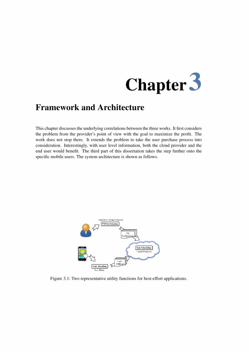
3.1 Two representative utility functions for best-effort applications . . . . . . . 13
4.1 Market pricing policy and its nonlinearity with memory usage . . . . . . . 214.2 Resource utilization: our approach vs. heuristic approaches . . . . . . . . . 284.3 Three representative job demand profiles . . . . . . . . . . . . . . . . . . . 304.4 Impact of reservation ratio to the revenue of combined algorithm . . . . . . 324.5 Impact of reservation ratio under different pricing models . . . . . . . . . . 33
5.1 Number of physical machines needed using each VM set selection scheme.Greedy-optimal is our VM selection in Section III . . . . . . . . . . . . . . 47
5.2 Two representative utility functions for best-effort applications . . . . . . . 495.3 Completion rate for inverse proportional function with 2048 physical ma-
chines and random VM selection for best-fit and first-fit . . . . . . . . . . . 505.4 Completion rate for inverse proportional function with 2048 physical ma-
chines and greedy-optimal VM selection for best-fit and first-fit . . . . . . . 515.5 Completion rate for linear drop function with 2048 physical machines and
random VM selection for best-fit and first-fit . . . . . . . . . . . . . . . . . 525.6 Completion rate for linear drop function with 2048 physical machines and
greedy-optimal VM selection for best-fit and first-fit . . . . . . . . . . . . . 535.7 Completion rate w.r.t. different cluster scales under inverse proportional
utility functions . . . . . . . . . . . . . . . . . . . . . . . . . . . . . . . . 545.8 CPU utilization ratio with 2048 under inverse proportional utility function . 545.9 Completion rate w.r.t. different deadlines under inverse proportional utility
function in a 2048 physical machine cluster . . . . . . . . . . . . . . . . . 555.10 Initial reservation threshold . . . . . . . . . . . . . . . . . . . . . . . . . . 55
6.1 Process of mobile cloud computing and the role of code partition . . . . . . 626.2 Overall performance in terms of end-to-end delay . . . . . . . . . . . . . . 63
List of Figures XII
6.3 Call Graph for a face recognition application. A 42kB jpeg is recognisedamong a set of 32 images of same size. White vertices (in contrast to greyones) indicate remotely executable methods; The number on the right handside of a method with underline and italics format is its execution time onserver side with the minimal amount of resource. Vertices are labelled withmillion CPU cycles of methods; Edges are labelled with sizes of input antreturn states . . . . . . . . . . . . . . . . . . . . . . . . . . . . . . . . . . 68
6.4 First feature of minimal offload property: once a node is to be run on theserver side, all its descendants should be run on the server . . . . . . . . . . 79
6.5 Second feature of minimal offload property: once a node is to be run on themobile side, its descendants that would run on the server are clustered . . . 80
6.6 Comparison of the optimal minimal time partition with call link based par-tition in terms of overall time . . . . . . . . . . . . . . . . . . . . . . . . . 80
6.7 Portion of methods run locally vs. user specified completion time . . . . . . 816.8 Portion of methods run on the server vs. user specified budget limit. As-
suming rent the basic unit for one minute be 100 . . . . . . . . . . . . . . . 816.9 Completion rate of the jobs with varying server capacity. Red line: mini-
mal feasible resource demand; blue line: minimal overall time partition inCloudNet . . . . . . . . . . . . . . . . . . . . . . . . . . . . . . . . . . . 82
List of Tables
4.1 Classification in All Dimensions . . . . . . . . . . . . . . . . . . . . . . . 244.2 Completion rate (market pricing model) . . . . . . . . . . . . . . . . . . . 304.3 Completion rate (linear pricing model) . . . . . . . . . . . . . . . . . . . . 304.4 Our combined algorithm vs. pure CP vs. 2D-best fit . . . . . . . . . . . . . 314.5 Performance with 3 different representative job profiles . . . . . . . . . . . 314.6 Summary: best reservation ratio in different parameters . . . . . . . . . . . 33
5.1 Application resource demand and VM & PM capacity . . . . . . . . . . . . 365.2 VM configurations (normalized to ) . . . . . . . . . . . . . . . . . . . . . 475.3 Utilization with different cluster scales for the two utility functions . . . . . 505.4 Comparison of overall utility with 2048 physical machines and inverse pro-
portional utility functions . . . . . . . . . . . . . . . . . . . . . . . . . . . 515.5 Our combined algorithm vs. pure CP . . . . . . . . . . . . . . . . . . . . . 525.6 Reservation Threshold with 2048 physical machines . . . . . . . . . . . . . 535.7 Reservation Threshold with 1024 physical machines . . . . . . . . . . . . . 54
6.1 Code Partition Efficiency . . . . . . . . . . . . . . . . . . . . . . . . . . . 74

Chapter1Introduction
Cloud computing provides tenants the resources and services in a pay-as-you-go manner nomatter when and where the requests are submitted. To support the submitted applicationsat a large scale, an efficient and effectively resource scheduling scheme is an important partto both cloud providers and tenants. This chapter would specify the resource schedulingproblem studied in this thesis.
In this section, the cloud scheduling problems are identified. To be specific, two steps aretaken in looking at the cloud scheduling problem. In the first step, this work considers theintra-cloud scheduling, where the cloud provider aims to improve the inter-VM fragmentsvia elaborately designing a problem-specific scheduling algorithm. In the second step, thiswork extends the vision into a world where user job resource demand is leveraged to furtherjointly reduce the intra-VM and inter-VM fragments.
Chapter 1 Introduction 2
1.1 Problem and Definitions: Cloud Resource Scheduling
The development of cloud computing offers the opportunity to deploy and use resizable,available, efficient, and scalable computation resources on demand. Users can request com-putation resources in terms of virtual machines (VM) provided by the cloud provider. Oncethe resources are allocated, the users would have the complete control of the computingresources. These resources are used to support various kinds of applications, such as onlinesocial networks, video streaming, search engine, email, and etc.
To efficiently and effectively schedule the user submitted applications over cloud datacenter is an important issue for application performance, system throughput, and resourceutilization. The workload of the cloud data center is tremendous. As stated in [2], oneach day, thousands of jobs are submitted to the public cloud and the peak rate wouldbe as high as tens of thousands scheduling requests per second. In the meanwhile, thesubmitted jobs are also quite diverse in terms of resource demand, duration, throughput,latency and jitter [61, 74]. The massive size and diverse resource demand characteristicsof the workloads make the scheduling process more difficult. Despite the effort by variousstudies to improve the physical machines’s energy efficiency, the energy consumption of thecurrent on-shelf physical machines is still not proportional to the load of the machine andthe lower the utilization rate is, the more energy would be wasted. Hence, low utilizationrate would result in a huge waste of data center energy. Furthermore, the revenue of thecloud provider will be lowered down since less workloads can be hosted.
Specifically, an efficient and effective cloud scheduler should satisfy the following re-quirements.
1. Accurate or near accurate decision. The scheduling decision is the key point forthe cloud throughput and utilization, hence accuracy is the main measurement of thecloud scheduler. This requirement would also be referred to as the effective require-ment of the cloud scheduler.
2. Fast, online scheduling. Since the scheduler needs to make tens of thousands ofscheduling decisions per second [2], scheduling speed would hence become an im-portant factor for online scheduling. This requirement would also be referred to asthe efficiency requirement of the cloud scheduler.
3. Compatible for heterogeneous workloads. The physical machines in the cloud datacenter could have various resource capacity. The cloud workload would also have dif-ferent resource demand, duration, and SLA requirements. The cloud scheduler shouldbe able to make the fast yet accurate scheduling decisions w.r.t the job characteristics.
3 1.1 Problem and Definitions: Cloud Resource Scheduling
The computation resources in public cloud are provided in various types of VMs andvarious ways of using this VMs. For example, as stated on its website [46], Amazon EC2provides General Purpose Instances like T2, M4 and M3; Compute Optimized Instances likeC4 and C3; Memory Optimized Instance like R3; GPU Instance like G2; Storage OptimizedInstances like I2 and D2. There are three ways of purchasing the instances (VMs), namely“On-Demand Instances, Reserved Instances and Spot Instances” [47].
To use the On-Demand Instances, users should purchase the VMs on an hourly basis.This is suitable for applications of short duration and spiky or unpredictable workloads.
To use the Reserved Instances, users should purchase the VMs with an upfront payment.They would then get a discount for the hourly fee. This is suitable for applications with longduration and steady workloads. By using Reserved Instances, it is possible for this kind ofapplications to save a lot of money.
The price of the Spot Instances is not constant but will fluctuate w.r.t the supply anddemand relationships. To use the Spot Instances, the users should provide a maximumamount of fee they would like to pay which is their bid and is usually lower than the priceof the On-Demand Instances. If the price of the Spot Instances goes lower than the user’sbid, AWS would allocate his/her the type and number of VMs they specified. If the theprice of the Spot Instances goes higher than the user’s bid, the allocated VMs would beshut down. Spot Instances is suitable for applications with flexible start times and is onlymeaningful at a low price.
However, there are some problems with the current VM based resource provisioning andpurchasing scheme.
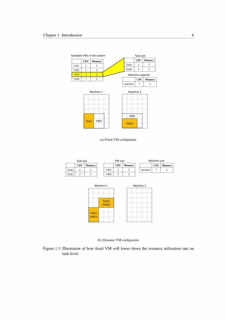
On the task level, the fixed VM configuration would lower down resource utilizationrate1. Although there are several VM types and configurations been provided, the actualnumber is still limited. Tenants need to choose among these limited configurations to caterto their resource demand. However, the resource could be wasted due to fixed VM config-uration. Fig. 1.1 shows an example of how the fixed configuration would lower down thethroughput.
In this example, there are two types of resources: CPU and memory. Let’s assume thereare four VM types with configurations and two tasks need to be allocated. The VM andphysical machine configurations and tasks’ resource demands are listed in the figure. If thetenants are able to estimate their resource demands accurately, both of the two tasks wouldchoose VM 3 to accommodate the workload. In this case, two physical machines are needed
1In this thesis, the term “task” is used to represent the minimum granularity of the workload that cannot besplit anymore; the term “applications” and “jobs” are used interchangeably to represent the tasks from thesame tenant
Chapter 1 Introduction 4
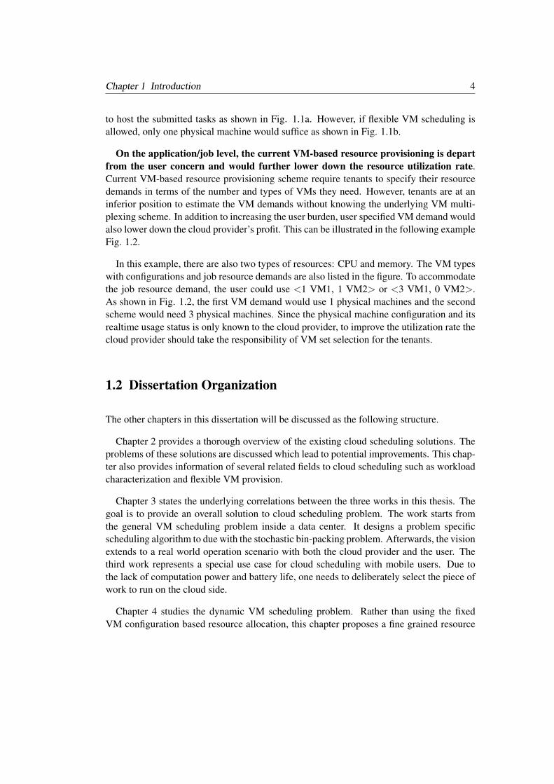
to host the submitted tasks as shown in Fig. 1.1a. However, if flexible VM scheduling isallowed, only one physical machine would suffice as shown in Fig. 1.1b.
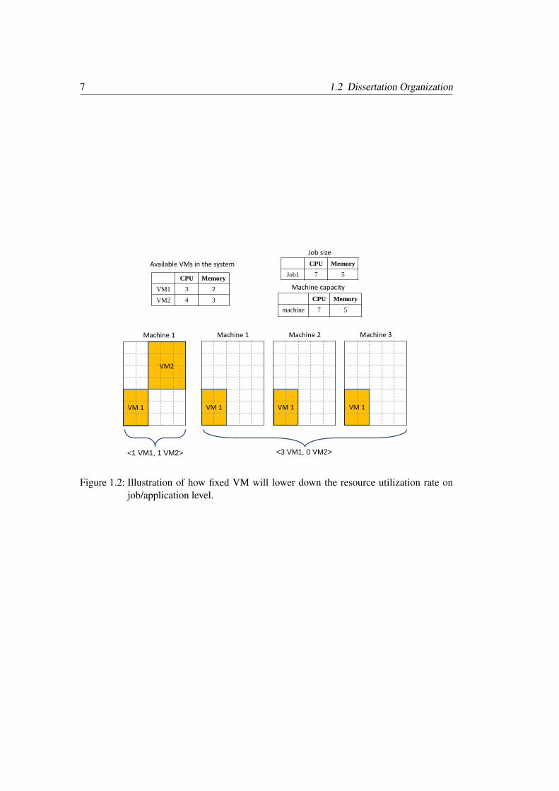
On the application/job level, the current VM-based resource provisioning is departfrom the user concern and would further lower down the resource utilization rate.Current VM-based resource provisioning scheme require tenants to specify their resourcedemands in terms of the number and types of VMs they need. However, tenants are at aninferior position to estimate the VM demands without knowing the underlying VM multi-plexing scheme. In addition to increasing the user burden, user specified VM demand wouldalso lower down the cloud provider’s profit. This can be illustrated in the following exampleFig. 1.2.
In this example, there are also two types of resources: CPU and memory. The VM typeswith configurations and job resource demands are also listed in the figure. To accommodatethe job resource demand, the user could use <1 VM1, 1 VM2> or <3 VM1, 0 VM2>.As shown in Fig. 1.2, the first VM demand would use 1 physical machines and the secondscheme would need 3 physical machines. Since the physical machine configuration and itsrealtime usage status is only known to the cloud provider, to improve the utilization rate thecloud provider should take the responsibility of VM set selection for the tenants.
1.2 Dissertation Organization
The other chapters in this dissertation will be discussed as the following structure.
Chapter 2 provides a thorough overview of the existing cloud scheduling solutions. Theproblems of these solutions are discussed which lead to potential improvements. This chap-ter also provides information of several related fields to cloud scheduling such as workloadcharacterization and flexible VM provision.
Chapter 3 states the underlying correlations between the three works in this thesis. Thegoal is to provide an overall solution to cloud scheduling problem. The work starts fromthe general VM scheduling problem inside a data center. It designs a problem specificscheduling algorithm to due with the stochastic bin-packing problem. Afterwards, the visionextends to a real world operation scenario with both the cloud provider and the user. Thethird work represents a special use case for cloud scheduling with mobile users. Due tothe lack of computation power and battery life, one needs to deliberately select the piece ofwork to run on the cloud side.
Chapter 4 studies the dynamic VM scheduling problem. Rather than using the fixedVM configuration based resource allocation, this chapter proposes a fine grained resource
5 1.2 Dissertation Organization
scheduling scheme where each VM is shaped into the size of the user workload. Areservation-based VM scheduling scheme is proposed. Experiment results show that theflexible VM scheduling scheme could substantially improve the utilization of the data cen-ter and the job completion rate. This chapter is based-on the work in [88].
Chapter 5 studies the joint VM scheduling and VM set selection problem. This chap-ter proposes a multi-resource scheduler that first translate the tenants’ resource demandi.,,R5ZXs; it then uses the reservation-based scheduling to allocate the VM sets onto physi-cal machines with the goal to achieve user SLA as well as to improve the overall utility. Anoptimal online VM set selection algorithm is designed to satisfy the user resource demandand reduce the number of activated physical machines.
Chapter 6 studies a use case of the cloud resource scheduling problem. This work extendsthe initial cloud resource scheduling problem to a mobile case, where the mobile users try toleverage the remote resource to execute its computational work. The system delays includeexecution time on both the client and server, the transmission between the parts, as well asthe code partition time on the server side. An optimal code partition algorithm is proposedand evaluations are done in real life environment. This chapter is based-on the work in [89].
Chapter 7 summarizes this work with a discussion of dissertation impact and future di-rections.
Chapter 1 Introduction 6
Task2
CPU Memory
VM1 1 2
VM2 2 2
VM3 3 4
VM4 7 5
Available VMs in the system
CPU Memory
Task1 2 3
Task2 3 2
Task size
CPU Memory
machine 7 5
Machine capacity
Task1 VM3
VM3
Machine 1 Machine 2
(a) Fixed VM configuratin.
CPU Memory
Task1 2 3
Task2 3 2
Task size
CPU Memory
machine 7 5
Machine size
Machine 1
CPU Memory
VM1 2 3
VM2 3 2
VM size
Machine 2
Task1(VM1)
Task2(VM2)
(b) Dynamic VM configuratin.
Figure 1.1: Illustration of how fixed VM will lower down the resource utilization rate ontask level.
7 1.2 Dissertation Organization
CPU Memory
VM1 3 2
VM2 4 3
Available VMs in the system CPU Memory
Job1 7 5
Job size
CPU Memory
machine 7 5
Machine capacity
Machine 1
VM2
Machine 1
VM 1 VM 1
Machine 2
VM 1
Machine 3
VM 1
<1 VM1, 1 VM2> <3 VM1, 0 VM2>
Figure 1.2: Illustration of how fixed VM will lower down the resource utilization rate onjob/application level.

Chapter2Background and Related Work
This chapter provides an overview of the state-of-the-art work of cloud scheduling andworkload characterization. It also presents the background knowledge and some terminolo-gies of cloud resource scheduling.
Chapter 2 Background and Related Work 10
2.1 Cloud Scheduling
The scale and impact of cloud data centers grow significantly during last decades. Largedata centers such as Amazon EC2 and Microsoft Azure, usually contain tens of thousands ofphysical machines with a sophisticated network topology. In the meanwhile, the workloadin cloud data center is heterogenous since it comes from various types and functions ofapplications. In a complicated system like this, it is usually difficult to develop scalablescheduling schemes to handle the enormous number and quite diverse jobs/tasks [60]. Tobe specific, it is hard for the cloud providers to make online decisions of which tasks shouldbe run on which physical machine at what time.
A number of solutions have been proposed for the scheduling problem in large scalecloud data centers [30] [19]. The ASRPT [60] approach can provide a scheduler with anaccuracy bound of two compared to the optimal solution. However, the scalability of AS-PRT is not good enough since it contains a sorting procedure whose time complexity growssignificantly w.r.t. the number of physical machines.
There are also some works that leverages the BvN [12] heuristic to design their schedul-ing policies. To use the BvN heuristic, one need to know the distribution of the arrival pro-cess. The scheduler could guarantee the queue stability by requiring an maximum waitingtime for each schedule in the BvN decomposition matrix. The problem with the BvN-basedschedulers is the maximum waiting time can be quite large and would grow significantlywith the number of ToR switches [11]. Hence the scalability of the BvN-based scheduler isnot good enough either.
There are also some other works that take the cloud pricing into their consideration. Thegoal is to maximize the provider profit [91] [90] or to improve the overall social welfare [92].The problem with this kind of works is that their auction policies are derived from empiricalstudies of spot instances which may not reflect the future interests of the cloud provider anduser.
2.2 Cloud Workload: Characterization and Prediction
A number of works have studied the public cloud workload characteristics [14]. [15] com-pares Amazon EC2 to several high-performance computing (HPC) clusters. [16] conductsa similar study that compares EC2 to NASA HPC cluster. Their finding is that the networkutilization in the public cloud is not as high as in operational clusters. [17] deploys severalnetworking benchmarks on Amazon EC2 and also finds that EC2 VMs has a lower resourceutilization ratio and higher variability than private scientific computation cloud. [18] finds
11 2.2 Cloud Workload: Characterization and Prediction
that heterogeneity of the physical machine hardware is the key factor that increases the per-formance variance. [13] provides a measurement study of resource usage patterns in EC2and Azure and finds out that a daily usage pattern.

Chapter3Framework and Architecture
This chapter discusses the underlying correlations between the three works. It first considersthe problem from the provider’s point of view with the goal to maximize the profit. Thework does not stop there. It extends the problem to take the user purchase process intoconsideration. Interestingly, with user level information, both the cloud provider and theend user would benefit. The third part of this dissertation takes the step further onto thespecific mobile users. The system architecture is shown as follows.
Figure 3.1: Two representative utility functions for best-effort applications.
Chapter 3 Framework and Architecture 14
3.1 Trace-driven VM Scheduling Algorithm
The first setting considers a scenario where the workload comes as individual tasks. Theaim of this work is to improve the cloud utilization by reducing the inter-VM fragments,which we called the external fragments.
The work starts from going through literature work when three different existing schedul-ing approaches are studied. The problem with these work is that they cannot balance be-tween the scheduling accuracy and scheduling speed. Hence, this work try to provide highcloud utilization within a reasonable scheduling time.
To better understand the problem specific scheduling input, a trace-driven analysis is doneto study the workload characteristic. The finding is that duration is the deterministic factorof task importance.
Therefore, this work proposes a combined constraint programming and heuristic algo-rithm. The constraint programming algorithm is used to provide an accurate schedulingresult for the long and important tasks. The heuristic algorithm is used to schedule the shortand less important tasks.
A trace-driven simulation is done to evaluate the scheduling algorithm. It is worth notic-ing that the solution is not restrict to the two heuristic been selected. Results show that thecombined algorithm can achieve around 18% CPU and memory utilization improvement.
3.2 Joint User and Cloud Scheduling
The second setting extends the vision to a real world cloud operation scenario where usershave to buy VM sets from the cloud provider. There exist multiple VM sets that can satisfythe user resource demand while not all of them would have the same quality. By delicatelychoosing the VM set for the users, the cloud provider would further improve its resourceutilization.
This part of work first illustrates why the low quality VM set would cause both internaland external fragments. Then it provides a solution to find the optimal VM set when thecloud users arrive as a stochastic process. It has be proved by theoretical analysis that theproposed algorithm can achieve global optimal.
15 3.3 Cloud Scheduling for Mobile Users
3.3 Cloud Scheduling for Mobile Users
The third setting discussed the mobile cloud scenario when the cloud users has more re-strict requirement for the timely response and local side energy saving. The work uses twoapplications namely the face recognition and natural language processing as examples toillustrate the joint cloud partition and resource scheduling problem.
This work proposes a scheme for multiple cloud users to share the common cloud infras-tructure. It contains a mobile to cloud code partition process and cloud resource schedulingprocess. Since the network condition will impact the state transmission between the mobileuser and the cloud provider, Instead of making an offloading decision on each node, thecode partition process transfers the call graph into a call link to get the optimal offloadingand integrating points.

Chapter4Deadline Aware Multi-Resource Schedulingin Cloud Data Center
This chapter considers the dynamic cloud resource scheduling problem on the task level.Cloud data centers typically require tenants to specify the resource demands for the virtualmachines (VMs) they create using a set of pre-defined, fixed configurations, to ease theresource allocation problem. Unfortunately, this leads to low resource utilization of clouddata center as tenants are obligated to conservatively predict the maximum resource demandof their applications.
The work in this chapter argues that instead of using a static VM resource allocation, thefiner-grained dynamic resource allocation and scheduling scheme can substantially improvethe utilization of the data center resources by increasing the number of tasks accommodatedand correspondingly, the cloud data center provider’s revenue.
The dynamic real-time scheduling of tasks can also ensure that the performance goalsfor the tenant VMs are achieved. Examining a typical publicly available cluster data centertrace, an observation is that the cloud workloads follows the 80/20 principle. A large numberof tasks are short and require and only a small proportion of tasks are long and which requiresubstantial compute or memory resources. This observation can be used to facilitate theresource scheduling algorithm design.
This work proposes an optimization based approach that exploits this division betweenthe short and long jobs to dynamically allocate a cloud data center’s resources to achievesignificantly better utilization by increasing the number of tasks accommodated by the datacenter.
The rest of the chapter is organized as follows. Section 4.1 gives an overview of thescheduling algorithms and resource allocation strategies. Section 4.2 presents the integerprogramming model to describe the scheduling problem. Section 4.3 provides our com-
Chapter 4 Deadline Aware Multi-Resource Scheduling in Cloud Data Center 18
bined constraint programming and heuristic solution. Simulation results and evaluationsare presented in Section 4.4. This chapter is summarized in Section 4.5.
19 4.1 Background and Motivation
4.1 Background and Motivation
Public cloud services are known for their flexibility to offer compute capability to enterpris-es and private users on a pay-as-you-go basis. It provides a variety of resources, such asCPU, memory, storage and network resource to tenants. An essential aspect of cloud com-puting is its potential to statistically multiplex user demands into a common shared physicalinfrastructure to improve efficiency. However, the average utilization of each active phys-ical machine in cloud data center is still relatively low. In an ideal case, cloud servicescould allow the tenants to dynamically request their computing resources just based ontheir instantaneous needs. However, this is not quite the case in reality. According to recentreports, the estimated utilization ratio of AWS data center is approximately 7% [7], whilethe utilization rate at a corporate datacenter is approximately 40% -60% [42]. Despite theeffort by various studies to improve the energy efficiency of physical machine, the energyconsumption of current on-shelf physical machines is still not proportional to its load, andthe lower the utilization rate is, the more energy would be wasted. Hence, low utilizationrate would result in a waste of datacenter energy. Furthermore, since less workloads can behosted in the system, the revenue of the cloud provider will be lowered down.
The efficiency of a cloud infrastructure relies heavily on the underlying resource alloca-tion mechanism. The de-facto policy adopted by today’s cloud operators is virtual machine(VM)- based resource allocation, where a cloud operator provides a set of pre-defined, fixedVM configurations. To get access to the resource, tenants need to choose among theselimited configurations and specify the time and number of VMs they need. The cloudoperator then allocates the corresponding resources to the tenants. One issue of this ap-proach is that users have to purchase the resources based on their estimation of each VM’smaximum resource demand. However, the average consumption is often lower than thepeak value, resulting in resource wastage. Recently, several proposals have been madefor resource scheduling of cloud infrastructures with an aim to improve the resource ef-ficiency [21, 61, 90]. However, the inherent problem of resource waste due to fixed VMconfiguration limits the gains.
This work argues that using finer-grained resource scheduling can benefit both the cloudoperator and the tenants. In addition to evaluation metrics of job completion rate and re-source utilization rate, we also consider the overall revenue of the cloud operator as theoptimization objective which can be seen as a direct reflection of the cloud operator’s in-terest. This also results in meeting the job’s deadline. With objective of maximizing therevenue and taking into account the data center’s capacity constraint, the multi-resourcescheduling problem is modeled as an integer programming problem. However, the tradi-tional integer programming solvers are not applicable here due to the strict requirement foronline resource scheduling to determine the solution quickly and schedule the job so that it
Chapter 4 Deadline Aware Multi-Resource Scheduling in Cloud Data Center 20
completes within the deadline. As summarized in [24], even for a very small scale of jobsand number of servers, the time to solve the problem would be unacceptable. For example,in one case tested with 4 machines and 22 jobs, the solution time is 1957.6 seconds on IntelXeon E5420 2.50 GHz computers with 6 MB cache and 6 GB memory.
The work analyzes the resource demands of jobs from a public cluster trace [49], andfind out that they have a clear relationship to the job duration. The relatively small numberof long duration jobs consume the majority of the computing resources. This motivates theapproach to get a tradeoff between scheduling accuracy and scheduling speed: since the fewlong duration jobs consume most of the resources, a sophisticated scheduling algorithm thatcan reach an optimal solution is used; on the other hand, for short duration jobs, due to theirlarge number, fast scheduling is important. Therefore, a combined constraint programmingand heuristic scheduling algorithm is proposed. We use constraint programming as the toolto find an optimal scheduling for the long duration jobs. For the jobs with short durations,our experiments show that simple heuristics such as first fit or best fit suffice.
4.2 System Model
This work models the multi-resource scheduling problem in a public cloud as an integerprogramming problem with an objective to maximize the overall revenue of cloud opera-tor. The overall revenue is defined to be the sum of the utility of jobs that have met theirdeadlines. For jobs that cannot get allocated, they do not contribute to the cloud operator’srevenue.
4.2.1 Pricing Policy
Multi-resource pricing is challenging for public cloud operators. Many approaches havebeen proposed to get a fair, profitable, and proportional pricing scheme for the multi-resource environment [84] [26] [27] [29]. Since the pricing policy is orthogonal to theresource scheduling problem, two simple pricing policies are used in this work, as present-ed below.
4.2.1.1 Market Pricing
The first pricing policy been used is the policy adopted by current cloud operators [48].Currently the Google Compute Engine provides 3 VM types, namely standard, high mem-ory and high CPU. The configurations that are not covered by the policy are calculated by
21 4.2 System Model
05
1015
20
0
50
100
1500
0.5
1
1.5
2
# of virtual coresMemory (GB)
Pric
e
(a) Interpolation of market pricing.
0 2 4 6 8 10 12 14 160
0.2
0.4
0.6
0.8
1
1.2
1.4
1.6
1.8
2
# of virtual cores
Pric
e
3.75 GB memory / virtual core6.5 GB memory / virtual core0.9 GB memory / virtual core
(b) Nonlinearity with memory.
Figure 4.1: Market pricing policy and its nonlinearity with memory usage.
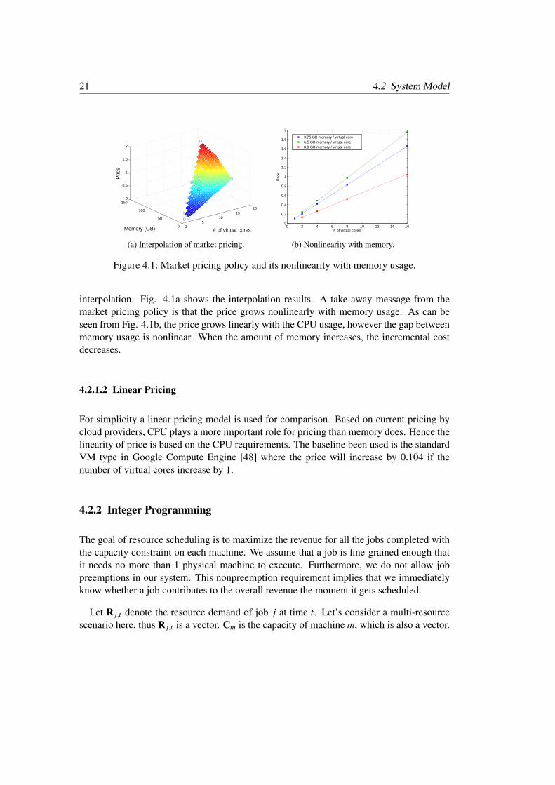
interpolation. Fig. 4.1a shows the interpolation results. A take-away message from themarket pricing policy is that the price grows nonlinearly with memory usage. As can beseen from Fig. 4.1b, the price grows linearly with the CPU usage, however the gap betweenmemory usage is nonlinear. When the amount of memory increases, the incremental costdecreases.
4.2.1.2 Linear Pricing
For simplicity a linear pricing model is used for comparison. Based on current pricing bycloud providers, CPU plays a more important role for pricing than memory does. Hence thelinearity of price is based on the CPU requirements. The baseline been used is the standardVM type in Google Compute Engine [48] where the price will increase by 0.104 if thenumber of virtual cores increase by 1.
4.2.2 Integer Programming
The goal of resource scheduling is to maximize the revenue for all the jobs completed withthe capacity constraint on each machine. We assume that a job is fine-grained enough thatit needs no more than 1 physical machine to execute. Furthermore, we do not allow jobpreemptions in our system. This nonpreemption requirement implies that we immediatelyknow whether a job contributes to the overall revenue the moment it gets scheduled.
Let R j,t denote the resource demand of job j at time t. Let’s consider a multi-resourcescenario here, thus R j,t is a vector. Cm is the capacity of machine m, which is also a vector.
Chapter 4 Deadline Aware Multi-Resource Scheduling in Cloud Data Center 22
Notice that the homogeneity property is not imposed on the resource capacity of machines.xm, j,t is a Boolean variable, where 1 indicates job j is assigned to machine m at time t and0 otherwise. Lm,t is the utilization vector of machine m at time t. All machines shouldn’texceed their capacities at anytime. D j is the deadline of job j while Fj is its finishing time.U j is the utility of job j. Let’s define U j to be the w j which is the revenue obtained for ajob j if it completes before its deadline and 0 otherwise. This leads to the following integerprogramming model:
max ∑j∈J
U j (4.2.1)
s.t.∑j∈J
R j,t × x j,m,t = Lm,t ∀m ∈M, t ∈ T (4.2.2)
∑j∈J
Lm,t ≤ Cm ∀m ∈M, t ∈ T (4.2.3)
x j,m,t ∈{
0,1}
(4.2.4)
∑m∈M
xm, j,t ∈{
0,1}∀ j ∈ J, t ∈ T (4.2.5)
∑t∈T,t>0
|x j,m,t − x j,m,t−1| ≤ 2 (4.2.6)
U j =
{w j Fj ≤ D j
0 Fj > D j(4.2.7)
4.3 Combined Constraint Programming and HeuristicAlgorithm
The combined problem of job scheduling with resource constraints and deadline require-ments is NP-hard [33]. There are two challenges that make the existing approaches usingan integer programming model impractical in this situation. One is that a global optimalsolution needs information (arrival time, resource demand) of future jobs, which wouldcause the system become non causal. Another is that unlike allocation problems, a schedul-ing problem requires an online solution. The scale and speed requirements are difficult toachieve by current integer linear programming solvers. Thus, a new approach is needed forthis multi-resource scheduling problem.
The scheme been adopted here is the reservation mechanism, a practical approach usedby parallel computing to provide more reliable service to high priority jobs [38]. It fits theproblem well since the portion of more privileged jobs is small and their duration is long;once they get accommodated, they usually occupy that resource for a while hence allow thescheduling engine enough time for the next iteration.
23 4.3 Combined Constraint Programming and Heuristic Algorithm
Constraint programming (CP) is a set of tools that provides a high performance solutionto constraint-based discrete variable problems using constraint propagation and decision-making based search. The optimization engine of CP software is a set of logical deductiveinferences rather than the relaxations techniques of integer programming algorithms. TheCP solutions for resource allocation and planning have been shown to be usually 10+ timesfaster than the integer programming solvers for resource scheduling [56, 78].
4.3.1 Trace Analysis
The Google Cluster Trace from a 12,000-machine cluster over about a month-long peri-od [49] is used in our study. The trace contains a trace of resource demand over time anda trace of machine availability. Resource requests and measurements are normalized to thelargest capacity of the resource on any machine in the trace (which is 1.0). Due to normal-ization, CPU and memory usage range from 0 to 1.
Efficient VM scheduling scheme would demand a thorough understanding of the resourceusage pattern of the submitted applications. The basic step of resource usage pattern anal-ysis is to accurately yet efficiently classify the workloads into groups. To get a clear un-derstanding of the workload features, the K-means (a multi-dimension statistical clusteringalgorithm) algorithm [74] is used to determine the classification of large and small in eachof the 3 dimensions of a job (CPU, memory and duration).
One extream direction for job classification is to define each job as a class. However thisapproach would cause a large number of classes when there are many jobs which is a typicalcase in public cloud. On the other extream direction, is to use single class, which wouldprovide no benefit for the resource scheduling problem. The tradeoff used here is to definetwo types on each of the resource dimensions.
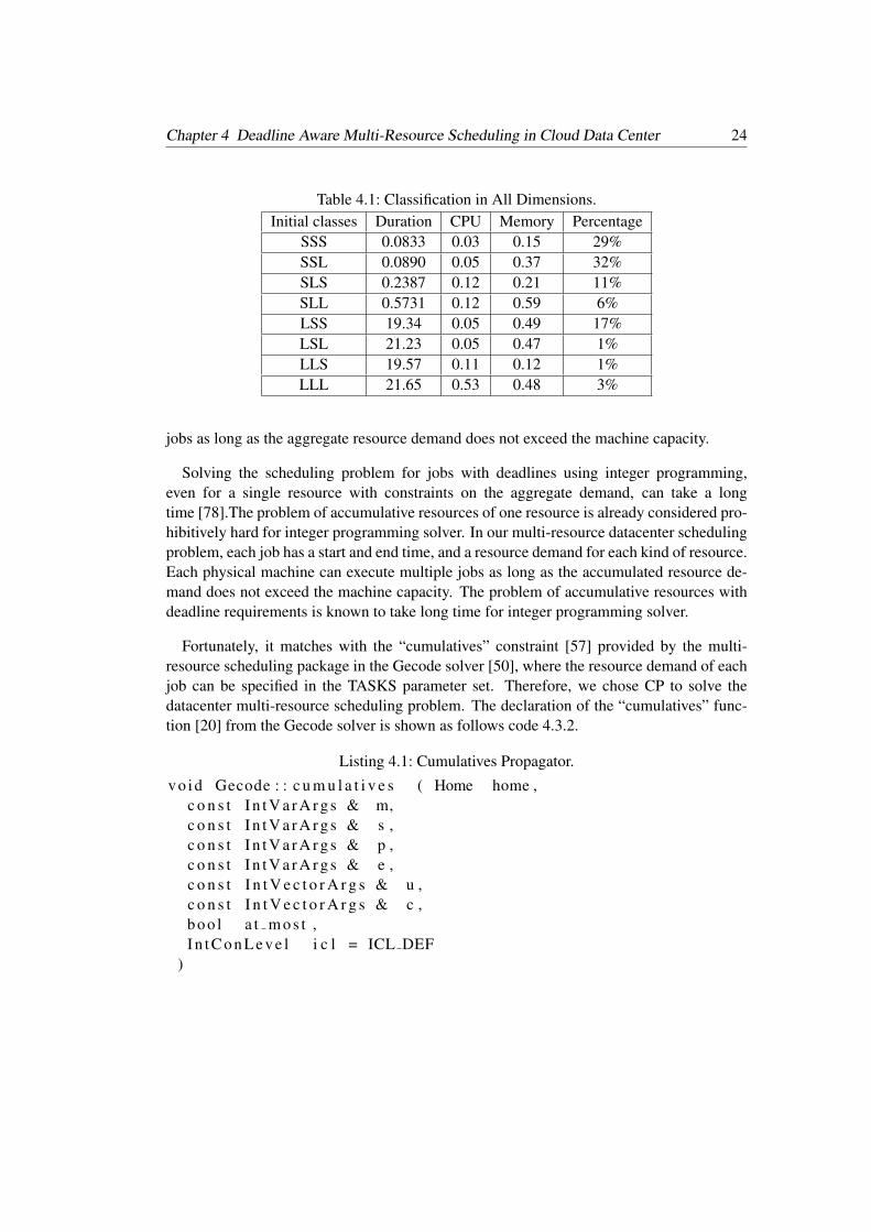
The initial 8 classes are summarized in Table 4.1. The numbers are the mean valuesof all jobs within that class and the unit of duration is hours. As can be seen from thetable, duration shows a clearer distinction of small and large than CPU and memory. Usingduration as the clustering factor, the jobs with a duration < 2.06 hours are classified as smallor short duration jobs, while those with a duration >= 2.06 hours are defined as large orlong duration jobs.
4.3.2 Constraint Programming and Gecode Solver
In our multi-resource datacenter scheduling problem, each job has a start and end time, anda resource demand for each kind of resource. Each physical machine can execute multiple
Chapter 4 Deadline Aware Multi-Resource Scheduling in Cloud Data Center 24
Table 4.1: Classification in All Dimensions.Initial classes Duration CPU Memory Percentage
SSS 0.0833 0.03 0.15 29%SSL 0.0890 0.05 0.37 32%SLS 0.2387 0.12 0.21 11%SLL 0.5731 0.12 0.59 6%LSS 19.34 0.05 0.49 17%LSL 21.23 0.05 0.47 1%LLS 19.57 0.11 0.12 1%LLL 21.65 0.53 0.48 3%
jobs as long as the aggregate resource demand does not exceed the machine capacity.
Solving the scheduling problem for jobs with deadlines using integer programming,even for a single resource with constraints on the aggregate demand, can take a longtime [78].The problem of accumulative resources of one resource is already considered pro-hibitively hard for integer programming solver. In our multi-resource datacenter schedulingproblem, each job has a start and end time, and a resource demand for each kind of resource.Each physical machine can execute multiple jobs as long as the accumulated resource de-mand does not exceed the machine capacity. The problem of accumulative resources withdeadline requirements is known to take long time for integer programming solver.
Fortunately, it matches with the “cumulatives” constraint [57] provided by the multi-resource scheduling package in the Gecode solver [50], where the resource demand of eachjob can be specified in the TASKS parameter set. Therefore, we chose CP to solve thedatacenter multi-resource scheduling problem. The declaration of the “cumulatives” func-tion [20] from the Gecode solver is shown as follows code 4.3.2.
Listing 4.1: Cumulatives Propagator.
vo id Gecode : : c u m u l a t i v e s ( Home home ,c o n s t I n t V a r A r g s & m,c o n s t I n t V a r A r g s & s ,c o n s t I n t V a r A r g s & p ,c o n s t I n t V a r A r g s & e ,c o n s t I n t V e c t o r A r g s & u ,c o n s t I n t V e c t o r A r g s & c ,boo l a t m o s t ,I n t C o n L e v e l i c l = ICL DEF
)
25 4.3 Combined Constraint Programming and Heuristic Algorithm
As stated in [20], in the “cumulatives” function, m denots the machine assigned to thejob; s is the start time assigned the job; p is the processing time of the job; e is the end timeassigned to the job; u is the amount of resources consumed by the job; c is the capacity ofeach machine; both u and c are vectors for each input.
Even though the CP solver is much faster than the integer linear programming solutionapproaches, it still cannot catch up with the pace of job arrival and departure events ofjust the long duration jobs. To speedup the search process, a technique is used to avoidrepeatedly visiting the same search point for each iteration. This work exploits the factthat no preemption is allowed in our system. Hence, a job runs to completion on the samemachine. Leveraging this property, the number of variables that need to be determined foreach iteration is reduced significantly. For example, the number variables is reduced from1,458,176 to 6,144 in one iteration.
4.3.3 Heuristic Algorithms
We use two basic 2-dimensional first fit and best fit algorithms as the heuristic for schedul-ing short jobs. While the corresponding 1-dimensional first fit and best fit algorithms arethoroughly studied and tested, the definition of their 2-dimensional counterparts is some-what more flexible in its definition to match the application scenario. We define the notionof 2-dimensional first fit and best fit in our scheduling problem as follows.
4.3.3.1 2-dimensional First Fit
In the 2-dimensional first fit, we assign an incoming job to the first machine that can executethe job within its capacity. In the 3-layer tree topology for the datacenter, we define the orderof assignment as being from the leftmost machine moving to the right.
4.3.3.2 2-dimensional Best Fit
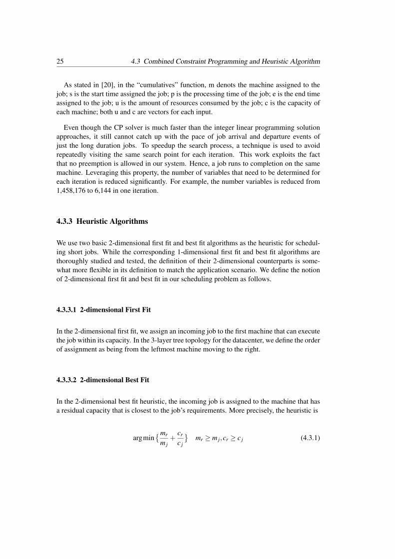
In the 2-dimensional best fit heuristic, the incoming job is assigned to the machine that hasa residual capacity that is closest to the job’s requirements. More precisely, the heuristic is
argmin{mr
m j+
cr
c j
}mr ≥ m j,cr ≥ c j (4.3.1)
Chapter 4 Deadline Aware Multi-Resource Scheduling in Cloud Data Center 26
4.3.4 Combined Algorithm
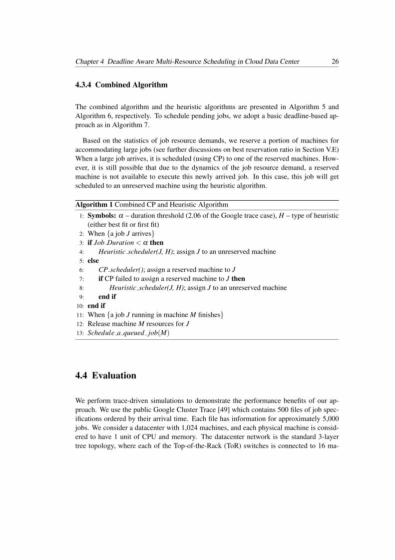
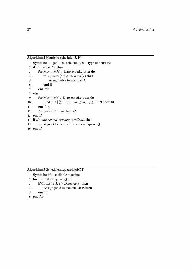
The combined algorithm and the heuristic algorithms are presented in Algorithm 5 andAlgorithm 6, respectively. To schedule pending jobs, we adopt a basic deadline-based ap-proach as in Algorithm 7.
Based on the statistics of job resource demands, we reserve a portion of machines foraccommodating large jobs (see further discussions on best reservation ratio in Section V.E)When a large job arrives, it is scheduled (using CP) to one of the reserved machines. How-ever, it is still possible that due to the dynamics of the job resource demand, a reservedmachine is not available to execute this newly arrived job. In this case, this job will getscheduled to an unreserved machine using the heuristic algorithm.
Algorithm 1 Combined CP and Heuristic Algorithm
1: Symbols: α – duration threshold (2.06 of the Google trace case), H – type of heuristic(either best fit or first fit)
2: When {a job J arrives}3: if Job Duration < α then4: Heuristic scheduler(J, H); assign J to an unreserved machine5: else6: CP scheduler(); assign a reserved machine to J7: if CP failed to assign a reserved machine to J then8: Heuristic scheduler(J, H); assign J to an unreserved machine9: end if
10: end if11: When {a job J running in machine M finishes}12: Release machine M resources for J13: Schedule a queued job(M)
4.4 Evaluation
We perform trace-driven simulations to demonstrate the performance benefits of our ap-proach. We use the public Google Cluster Trace [49] which contains 500 files of job spec-ifications ordered by their arrival time. Each file has information for approximately 5,000jobs. We consider a datacenter with 1,024 machines, and each physical machine is consid-ered to have 1 unit of CPU and memory. The datacenter network is the standard 3-layertree topology, where each of the Top-of-the-Rack (ToR) switches is connected to 16 ma-
27 4.4 Evaluation
Algorithm 2 Heuristic scheduler(J, H)1: Symbols: J – job to be scheduled, H – type of heuristic2: if H = First Fit then3: for Machine M ∈ Unreserved cluster do4: if Capacity(M)≥ Demand(J) then5: Assign job J to machine M6: end if7: end for8: else9: for MachineM ∈ Unreserved cluster do
10: Find min{mr
m j+ cr
c j
}mr ≥ m j,cr ≥ c j; 2D-best fit
11: end for12: Assign job J to machine M13: end if14: if No unreserved machine available then15: Insert job J to the deadline-ordered queue Q16: end if
Algorithm 3 Schedule a queued job(M)
1: Symbols: M – available machine2: for Job J ∈ job queue Q do3: if Capacity(M)≥ Demand(J) then4: Assign job J to machine M return5: end if6: end for
Chapter 4 Deadline Aware Multi-Resource Scheduling in Cloud Data Center 28
0 200 400 600 800 10000.2
0.3
0.4
0.5
0.6
0.7
0.8
Time(s)
CP
U U
tiliz
atio
n
Combined Algorithm2D−Best FitVM−based
(a) CPU utilization.
0 200 400 600 800 10000.3
0.4
0.5
0.6
0.7
0.8
0.9
1
Time(s)
Mem
ory
Util
izat
ion
Combined Algorithm2D−Best FitVM−based
(b) Memory utilization.
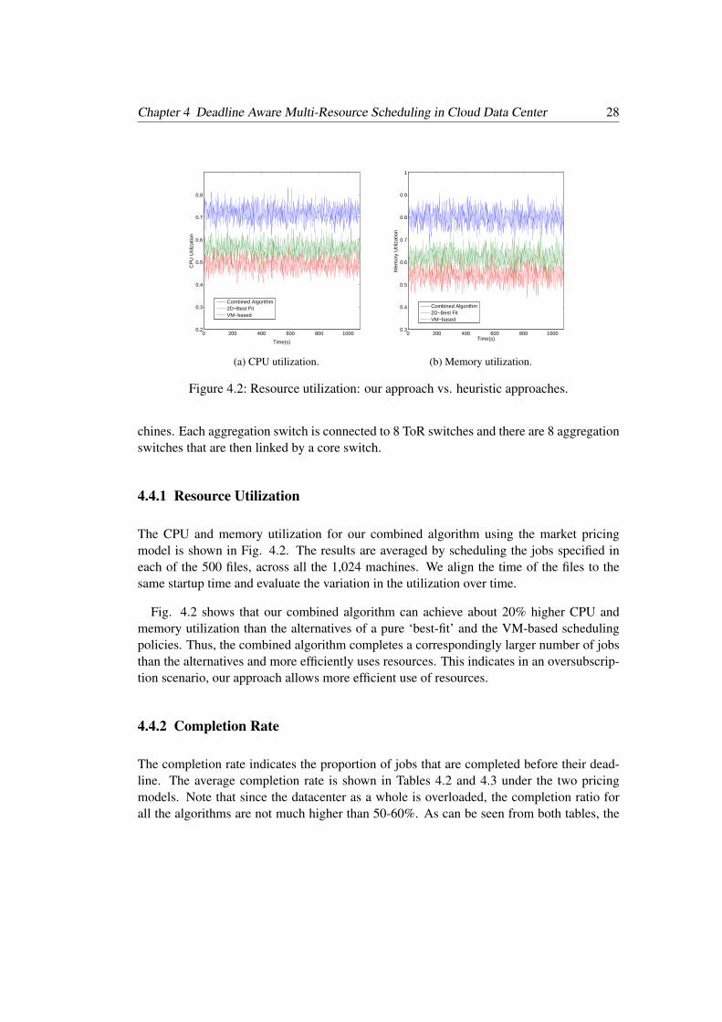
Figure 4.2: Resource utilization: our approach vs. heuristic approaches.
chines. Each aggregation switch is connected to 8 ToR switches and there are 8 aggregationswitches that are then linked by a core switch.
4.4.1 Resource Utilization
The CPU and memory utilization for our combined algorithm using the market pricingmodel is shown in Fig. 4.2. The results are averaged by scheduling the jobs specified ineach of the 500 files, across all the 1,024 machines. We align the time of the files to thesame startup time and evaluate the variation in the utilization over time.
Fig. 4.2 shows that our combined algorithm can achieve about 20% higher CPU andmemory utilization than the alternatives of a pure ‘best-fit’ and the VM-based schedulingpolicies. Thus, the combined algorithm completes a correspondingly larger number of jobsthan the alternatives and more efficiently uses resources. This indicates in an oversubscrip-tion scenario, our approach allows more efficient use of resources.
4.4.2 Completion Rate
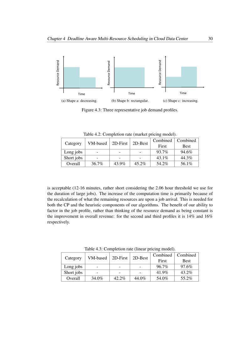
The completion rate indicates the proportion of jobs that are completed before their dead-line. The average completion rate is shown in Tables 4.2 and 4.3 under the two pricingmodels. Note that since the datacenter as a whole is overloaded, the completion ratio forall the algorithms are not much higher than 50-60%. As can be seen from both tables, the
29 4.4 Evaluation
proposed combined algorithm can improve the overall completion rate, especially for largejobs. This result reflects the fact that large jobs can use both the reserved resources and theunreserved resources. The completion ratio for the short jobs is significantly lower, showingthe effectiveness of the scheduling with reservations for the large jobs.
4.4.3 Comparison to Pure CP and Pure Heuristic Algorithms
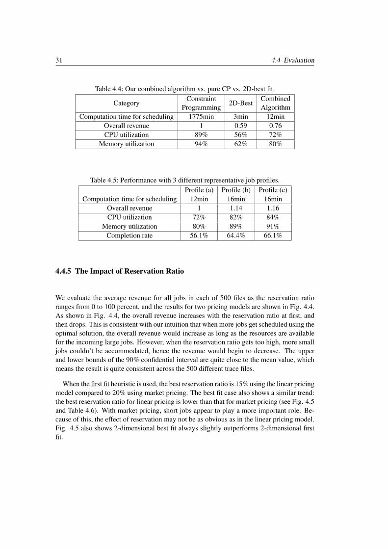
Table 4.4 compares our combined algorithm at its best reservation ratio against a pure Con-straint Programming algorithm or a pure heuristic (2-dimensional best fit). The overallrevenue is normalized with respect to the pure CP solution for comparison purposes. Thecomputation time for scheduling is estimated based on running the algorithm on a work-station with quad-core 2.0GHz processor and 16GB RAM. Since the CP simulation takes along time and all traces are of a similar nature, we compare the performance on one typicaltrace out of the 500 traces. As can be seen from the table, although CP can achieve the bestperformance, its time complexity makes the approach impractical. Our combined algorithmon the other hand, can provide reasonably good results within a short amount of time forscheduling (12 minutes for our combined algorithm, 3 minutes for heuristic and 1,775 min-utes or 29.6 hours for the pure CP). Our combined algorithm improves the overall revenue:going from 0.59 for the 2-dimensional best fit heuristic to 0.76 (28.8% increase). It is only24% lower than CP. Finally, our algorithm improves the CPU utilization (28.6% higher thanheuristic) and memory utilization (29% higher than heuristic).
4.4.4 Impact of Job Demand Profile
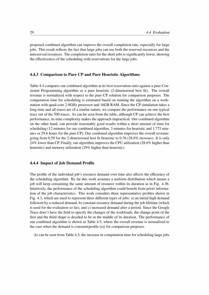
The profile of the individual job’s resource demand over time also affects the efficiency ofthe scheduling algorithm. By far this work assumes a uniform distribution which means ajob will keep consuming the same amount of resource within its duration as in Fig. 4.3b.Intuitively, the performance of the scheduling algorithm could benefit from priori informa-tion of the job characteristics. This work considers three representative profiles shown inFig. 4.3, which are used to represent three different types of jobs: a) an initial high demandfollowed by a reduced demand, b) constant resource demand during the job lifetime (whichis used for the evaluation so far), and c) increased demand after a period. Since the GoogleTrace does’t have the field to specify the changes of the workloads, the change point of thefirst and the third shape is decided to be in the middle of its duration. The performance ofour combined algorithm is shown in Table 4.5, where the overall revenue is normalized tothe case when the demand is constant(profile (a)) for comparison purposes.
As can be seen from Table 4.5, the increase in computation time for scheduling large jobs
Chapter 4 Deadline Aware Multi-Resource Scheduling in Cloud Data Center 30
Time
Res
ou
rce
Dem
and
(a) Shape a: decreasing.
Time
Res
ou
rce
Dem
and
(b) Shape b: rectangular.
Time
Res
ou
rce
Dem
and
(c) Shape c: increasing.
Figure 4.3: Three representative job demand profiles.
Table 4.2: Completion rate (market pricing model).
Category VM-based 2D-First 2D-BestCombined
FirstCombined
BestLong jobs - - - 93.7% 94.6%Short jobs - - - 43.1% 44.3%
Overall 36.7% 43.9% 45.2% 54.2% 56.1%
is acceptable (12-16 minutes, rather short considering the 2.06 hour threshold we use forthe duration of large jobs). The increase of the computation time is primarily because ofthe recalculation of what the remaining resources are upon a job arrival. This is needed forboth the CP and the heuristic components of our algorithms. The benefit of our ability tofactor in the job profile, rather than thinking of the resource demand as being constant isthe improvement in overall revenue: for the second and third profiles it is 14% and 16%respectively.
Table 4.3: Completion rate (linear pricing model).
Category VM-based 2D-First 2D-BestCombined
FirstCombined
BestLong jobs - - - 96.7% 97.6%Short jobs - - - 41.9% 43.2%
Overall 34.0% 42.2% 44.0% 54.0% 55.2%
31 4.4 Evaluation
Table 4.4: Our combined algorithm vs. pure CP vs. 2D-best fit.
CategoryConstraint
Programming2D-Best
CombinedAlgorithm
Computation time for scheduling 1775min 3min 12minOverall revenue 1 0.59 0.76CPU utilization 89% 56% 72%
Memory utilization 94% 62% 80%
Table 4.5: Performance with 3 different representative job profiles.Profile (a) Profile (b) Profile (c)
Computation time for scheduling 12min 16min 16minOverall revenue 1 1.14 1.16CPU utilization 72% 82% 84%
Memory utilization 80% 89% 91%Completion rate 56.1% 64.4% 66.1%
4.4.5 The Impact of Reservation Ratio
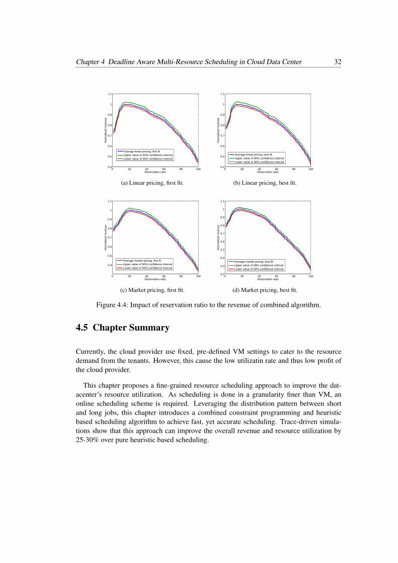
We evaluate the average revenue for all jobs in each of 500 files as the reservation ratioranges from 0 to 100 percent, and the results for two pricing models are shown in Fig. 4.4.As shown in Fig. 4.4, the overall revenue increases with the reservation ratio at first, andthen drops. This is consistent with our intuition that when more jobs get scheduled using theoptimal solution, the overall revenue would increase as long as the resources are availablefor the incoming large jobs. However, when the reservation ratio gets too high, more smalljobs couldn’t be accommodated, hence the revenue would begin to decrease. The upperand lower bounds of the 90% confidential interval are quite close to the mean value, whichmeans the result is quite consistent across the 500 different trace files.
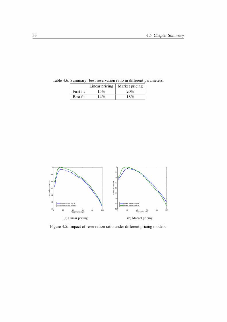
When the first fit heuristic is used, the best reservation ratio is 15% using the linear pricingmodel compared to 20% using market pricing. The best fit case also shows a similar trend:the best reservation ratio for linear pricing is lower than that for market pricing (see Fig. 4.5and Table 4.6). With market pricing, short jobs appear to play a more important role. Be-cause of this, the effect of reservation may not be as obvious as in the linear pricing model.Fig. 4.5 also shows 2-dimensional best fit always slightly outperforms 2-dimensional firstfit.
Chapter 4 Deadline Aware Multi-Resource Scheduling in Cloud Data Center 32
0 20 40 60 80 1000.4
0.5
0.6
0.7
0.8
0.9
1
1.1
Reservation ratio
Nor
mal
ized
rev
enue
Average linear pricing, first fitUpper value of 90% confidence intervalLower value of 90% confidence interval
(a) Linear pricing, first fit.
0 20 40 60 80 1000.4
0.5
0.6
0.7
0.8
0.9
1
1.1
Reservation ratio
Nor
mal
ized
rev
enue
Average linear pricing, best fitUpper value of 90% confidence intervalLower value of 90% confidence interval
(b) Linear pricing, best fit.
0 20 40 60 80 100
0.4
0.5
0.6
0.7
0.8
0.9
1
1.1
Reservation ratio
Nor
mal
ized
rev
enue
Average market pricing, first fitUpper value of 90% confidence intervalLower value of 90% confidence interval
(c) Market pricing, first fit.
0 20 40 60 80 1000.2
0.3
0.4
0.5
0.6
0.7
0.8
0.9
1
1.1
Reservation ratio
Nor
mal
ized
rev
enue
Average market pricing, best fitUpper value of 90% confidence intervalLower value of 90% confidence interval
(d) Market pricing, best fit.
Figure 4.4: Impact of reservation ratio to the revenue of combined algorithm.
4.5 Chapter Summary
Currently, the cloud provider use fixed, pre-defined VM settings to cater to the resourcedemand from the tenants. However, this cause the low utilizatin rate and thus low profit ofthe cloud provider.
This chapter proposes a fine-grained resource scheduling approach to improve the dat-acenter’s resource utilization. As scheduling is done in a granularity finer than VM, anonline scheduling scheme is required. Leveraging the distribution pattern between shortand long jobs, this chapter introduces a combined constraint programming and heuristicbased scheduling algorithm to achieve fast, yet accurate scheduling. Trace-driven simula-tions show that this approach can improve the overall revenue and resource utilization by25-30% over pure heuristic based scheduling.
33 4.5 Chapter Summary
Table 4.6: Summary: best reservation ratio in different parameters.Linear pricing Market pricing
First fit 15% 20%Best fit 14% 18%
0 20 40 60 80 1000.4
0.5
0.6
0.7
0.8
0.9
1
Reservation ratio
Nor
mal
ized
rev
enue
Linear pricing, first fitLinear pricing, best fit
(a) Linear pricing.
0 20 40 60 80 1000.2
0.3
0.4
0.5
0.6
0.7
0.8
0.9
1
Reservation ratio
Nor
mal
ized
rev
enue
Market pricing, first fitMarket pricing, best fit
(b) Market pricing.
Figure 4.5: Impact of reservation ratio under different pricing models.

Chapter5VM Set Selection
Current cloud resource allocation schemes usually require the tenants to specify their re-source demand in terms of the number of VMs in spite of the fact that the tenants are at aninferior position to estimate the VM demands. This chapter shows that there may exist mul-tiple VM sets that can support an application’s resource demand and by elaborately selectan appropriate VM set, the utilization of the data center can be improved without violatingthe application’s SLA.
This chapter proposes a multi-resource scheduler that allocates applications to VM setsand then to physical machines with the goal to achieve user SLA and to improve the overallutility. This work contains four parts: 1. an optimal online VM set selection scheme satisfy-ing the user resource demand and minimizing the number of activated physical machines; 2.an integer programming model to maximize the overall utility of the cloud provider underthe capacity constraint; 3. a reservation-based combined constraint programming approachto the problem; 4. a trace driven simulation to evaluate our VM set selection and VMscheduling approach.
The rest of the chapter is organized as follows. Section 5.1 and 5.2 illustrates the VMset selection and scheduling problem and presents the system model respectively. Section5.3 provides a greedy algorithm to select the VM set for each application. The proof of itsoptimality is in both the static and dynamic scenario. Simulation results and evaluations arepresented in Section 5.4. This chapter is concluded with discussions on some open issuesin Section .
Chapter 5 VM Set Selection 36
Table 5.1: Application resource demand and VM & PM capacity.
Res1 Res2App1 15 13App2 6 14VM1 5 3VM2 2 4
PM 7 7
5.1 Background and Motivation
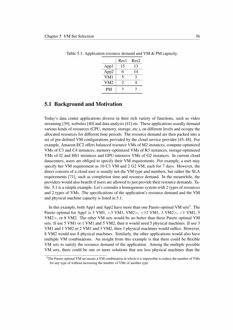
Today’s data center applications diverse in their rich variety of functions, such as videostreaming [39], websites [40] and data analysis [41] etc. These applications usually demandvarious kinds of resources (CPU, memory, storage, etc.), on different levels and occupy theallocated resources for different time periods. The resource demand are then packed into aset of pre-defined VM configurations provided by the cloud service provider [45, 48]. Forexample, Amazon EC2 offers balanced resource VMs of M2 instances, compute-optimizedVMs of C3 and C4 instances, memory-optimized VMs of R3 instances, storage-optimizedVMs of I2 and HS1 instances and GPU-intensive VMs of G2 instances. In current clouddatacenters, users are obliged to specify their VM requirements. For example, a user mayspecify her VM requirement as 10 C3 VM and 2 G2 VM, each for 7 days. However, thedirect concern of a cloud user is usually not the VM type and numbers, but rather the SLArequirements [71], such as completion time and resource demand. In the meanwhile, theproviders would also benefit if users are allowed to just provide their resource demands. Ta-ble. 5.1 is a simple example. Let’s consider a homogenous system with 2 types of resourcesand 2 types of VMs. The specifications of the application’s resource demand and the VMand physical machine capacity is listed in 5.1.
In this example, both App1 and App2 have more than one Pareto optimal VM sets2. ThePareto optimal for App1 is 5 VM1, <3 VM1, VM2>, <12 VM1, 3 VM2>, <1 VM1, 5VM2>, or 8 VM2. The other VM sets would be no better than these Pareto optimal VMsets. If use 5 VM1 or 1 VM1 and 5 VM2, then it would need 5 physical machines. If use 3VM1 and 1 VM2 or 2 VM1 and 3 VM2, then 3 physical machines would suffice. However,8 VM2 would use 8 physical machines. Similarly, the other applications would also havemultiple VM combinations. An insight from this example is that there could be flexibleVM sets to satisfy the resource demand of the application. Among the multiple possibleVM sets, there could be one or more solutions that use less physical machines than the
2The Pareto optimal VM set means a VM combination in which it is impossible to reduce the number of VMsfor any type of without increasing the number of VMs of another type.
37 5.1 Background and Motivation
others. By elaborately select an appropriate VM set, the utilization of the data center can beimproved.
Recent studies like [58, 61, 70, 74, 79] show that the applications run on cloud have di-verse service level requirements in terms of throughput, latency, and jitter. They furtherillustrate that the applications can be coarsely classified into two types: deadline-sensitiveapplications and best-effort applications [61,70,80]. The deadline-sensitive applications of-ten consume large amount of resource and have long durations. Furthermore, they are oftencritical to business, and have strict deadline requirements. The best-effort applications typi-cally consume less resource and do not have explicit deadlines. However, finishing the job atan earlier time would improve the users’ satisfaction. Hence we propose a cloud schedulingsystem aiming at guaranteeing the deadline requirements of the deadline-sensitive applica-tions as well as to improve the completion time of the best-effort applications. Throughextensive trace-driven analysis, we find that the number and the resource consumption ofthe deadline-sensitive and best-effort applications follows the 80/20 principle. While ma-jority of these applications are best-effort applications, up to 80% of the cloud data centerresource is consumed by deadline-sensitive applications [61, 74, 79]. We will leverage thisproperty to design an efficient resource scheduling algorithm later.
In this chapter, it is shown that the multiple Pareto optimal VM set property of the appli-cations can be used to improve the overall utilization of the system. We propose a multi-resource scheduler that allocates applications to VM sets and then to physical machines withthe goal to minimize the number of activated physical machines as well as to maximize theoverall utility. The utility function of the deadline-sensitive applications is defined as a 1-0function where the utility would stay the same when it is within its deadline and drop to zerowhen the it exceeds its deadline. For the best-effort applications, a soft utility function isused where the utility drops gradually [70]. This chapter first provides a greedy yet optimalalgorithm to find the VM set that can minimize the activated physical machines and stillsatisfy the resource requirement. Using the VM sets as input, we model the VM schedulingproblem as an integer programming problem with the goal to improve the overall utilityof all applications. By leveraging the 80/20 property of the deadline-sensitive applicationsand best-effort applications, we propose a combined constraint programming and heuristicalgorithm. We reserve a dynamic number of physical machines for the deadline-sensitiveapplications and use constraint programming to get a more accurate scheduling result. Dueto the huge number and the less resource consumption of the best-effort applications, weuse heuristic scheduling policy to get a fast yet acceptable scheduling result. Trace drivensimulation shows over 25% improvement of the overall utility compared to best-fit and first-fit using the optimal VM selection algorithm, over 30% improvement compared to best-fitand first-fit using random VM selection scheme and 18% improvement compared to theBazaar-I approach.
Chapter 5 VM Set Selection 38
The main contributions of this chapter are summarized as follows:
1. according to recent studies of cloud workload heterogeneity, we classify the userapplications into two types, namely deadline-sensitive applications and best-effortapplications. We demonstrate that allowing application specific SLA would improvethe cloud utilization and in the meanwhile guarantee the application performance.
2. we illustrate the multiple VM combination problem of application-aware schedulingand propose a greedy algorithm to choose the optimal VM combination in the senseof minimizing the activated physical machines
3. we develop a combined constrained programming scheduling algorithm exploringthe 80/20 property of the two types of cloud workload which provides an accuratescheduling for deadline-sensitive applications and fast yet acceptable scheduling forbest-effort applications
4. we use trace-driven simulation to evaluate our algorithm with comparison of both theVM set selection and scheduling algorithm.
5.2 VM Set Selection and Scheduling Model
This section illustrates the VM set selection and scheduling problem which aims to satisfythe user resource demand, meanwhile minimizing the number of activated physical ma-chines. We first identify the user SLA requirements of two types of applications and thenprovide a model to minimize the activated physical machines while satisfying the resourcedemand. After that, we present the overall model aiming to improve the utility over all theapplications.
5.2.1 User SLA Requirement and Utility Function
There are two aspects considered for SLA requirements of an applications:
1. resource demand and duration: an application use resource bundle [61], such as<16GB memory, 2 2.60GHZ CPUs, 100G SSD, 2 hours> to specify its resourcedemand. Both deadline-sensitive and best-effort applications should provide theirresource demands and durations.
2. deadline requirement: each deadline-sensitive applications would provide an exactdeadline associated with its resource demand. The best-effort applications do not
39 5.2 VM Set Selection and Scheduling Model
have such requirements.
In addition to the SLA requirements, each application has a utility function which de-pends on the completion time. For the deadline-sensitive applications, we use a 1-0 utilityfunction which drops directly to zero after the deadline. As for best-effort applications, weallow different types of decreasing functions [70].
5.2.2 Minimizing Active Physical Machines
Without loosing generality, let’s assume there are R types of resources and I types of VMsin the cloud system where {V M1,V M2, ...,V MI} denote the I types of VMs. The capacityof the type i VM on each type of resources is (bi,1,bi,2, ...,bi,R) while the capacity of thephysical machine is (c1,c2, ...,cR).
For each application, a feasible VM set should be able to support its resource demand onevery resource dimension. Assume for application k, the resource demand for type r is ak,r,and xi,k is the number of V Mi allocated to that application. Hence, the resource demand forapplication k would be:
I
∑i=1
bi,r× xi,k ≥ ak,r ∀r ∈ {1,2, ...,R} ,k ∈ {1,2, ...,K} (5.2.1)
Assume we have M physical machines and K applications in total. For each physicalmachine, the VMs allocated to that physical machine should not exceed its capacity on everyresource dimension. Let zi be the number of type i VM allocated on a physical machine.Then the capacity constraint on that physical machine would be,
I
∑i=1
bi,r× zi ≤ cr ∀r ∈ {1,2, ...,R} (5.2.2)
Actually, the capacity of a physical machine can be calculated in a simple way. In asystem of I types of VMs, the maximum number of VM1 that can be accommodated on aphysical machine would be min{ c1
b1,1, c2
b1,2, ... cR
b1,R}, which is the case when only VM1 and no
other VMs are allocated. Similarly, the maximum number of VM2 that can be accommo-dated on a physical machine would be min{ c1
b2,1, c2
b2,2, ... cR
b2,R}. More generally, the maximum
number of V Mi would be mini≤I,r≤R{ cibi,r}. Let’s denote vi to be the maximum number of
V Mi that can be hold on a single physical machine (which means vi = mini≤I,r≤R{ cibi,r}).
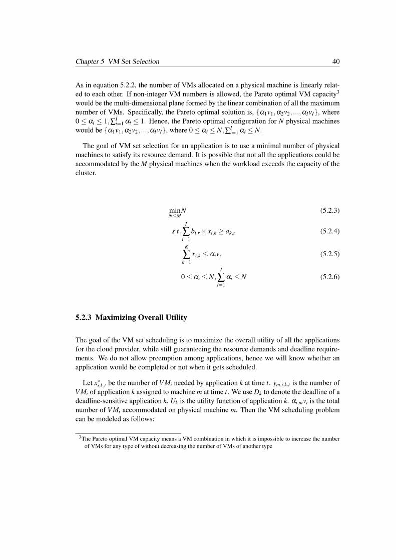
Chapter 5 VM Set Selection 40
As in equation 5.2.2, the number of VMs allocated on a physical machine is linearly relat-ed to each other. If non-integer VM numbers is allowed, the Pareto optimal VM capacity3
would be the multi-dimensional plane formed by the linear combination of all the maximumnumber of VMs. Specifically, the Pareto optimal solution is, {α1v1,α2v2, ...,αIvI}, where0 ≤ αi ≤ 1,∑I
i=1 αi ≤ 1. Hence, the Pareto optimal configuration for N physical machineswould be {α1v1,α2v2, ...,αIvI}, where 0≤ αi ≤ N,∑I
i=1 αi ≤ N.
The goal of VM set selection for an application is to use a minimal number of physicalmachines to satisfy its resource demand. It is possible that not all the applications could beaccommodated by the M physical machines when the workload exceeds the capacity of thecluster.
minN≤M
N (5.2.3)
s.t.I
∑i=1
bi,r× xi,k ≥ ak,r (5.2.4)
K
∑k=1
xi,k ≤ αivi (5.2.5)
0≤ αi ≤ N,I
∑i=1
αi ≤ N (5.2.6)
5.2.3 Maximizing Overall Utility
The goal of the VM set scheduling is to maximize the overall utility of all the applicationsfor the cloud provider, while still guaranteeing the resource demands and deadline require-ments. We do not allow preemption among applications, hence we will know whether anapplication would be completed or not when it gets scheduled.
Let x∗i,k,t be the number of V Mi needed by application k at time t. ym,i,k,t is the number ofV Mi of application k assigned to machine m at time t. We use Dk to denote the deadline of adeadline-sensitive application k. Uk is the utility function of application k. αi,mvi is the totalnumber of V Mi accommodated on physical machine m. Then the VM scheduling problemcan be modeled as follows:
3The Pareto optimal VM capacity means a VM combination in which it is impossible to increase the numberof VMs for any type of without decreasing the number of VMs of another type
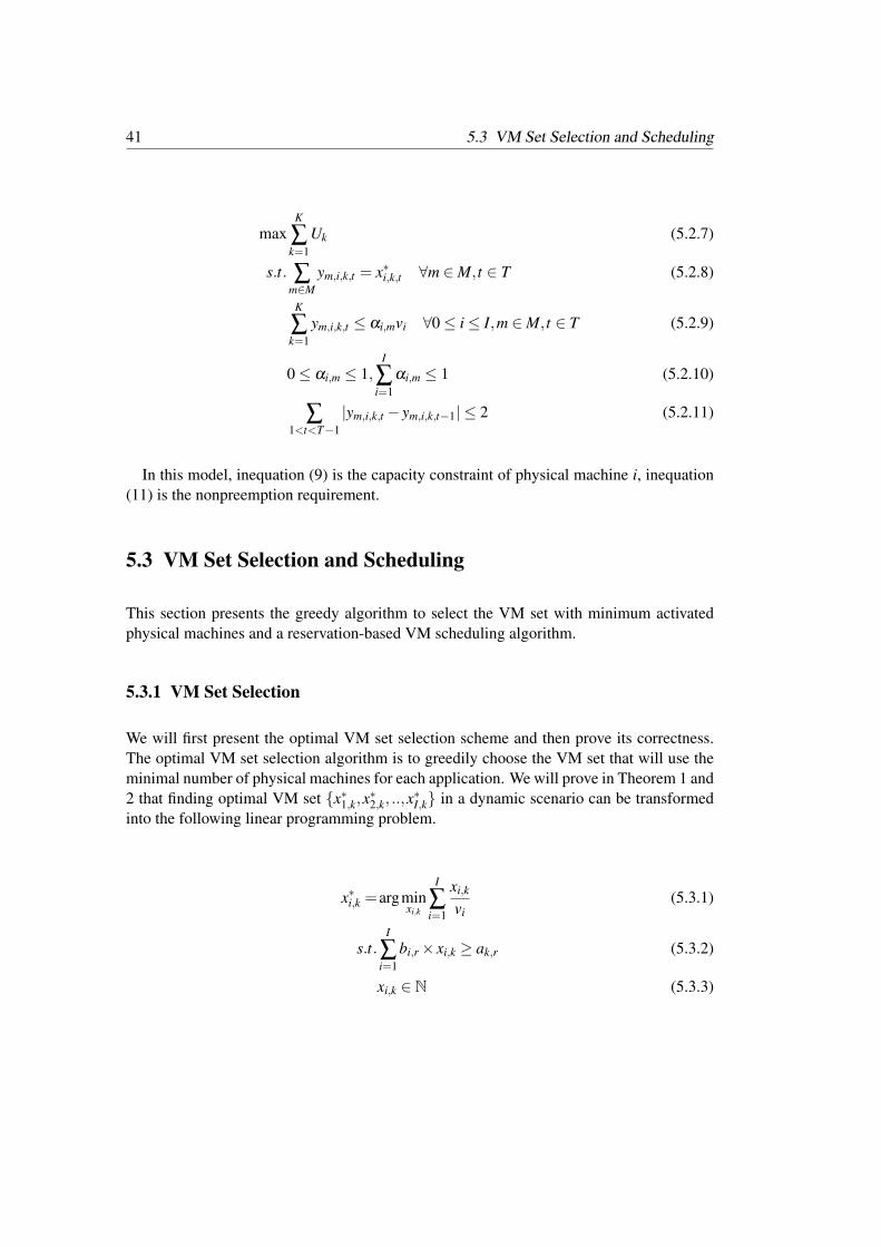
41 5.3 VM Set Selection and Scheduling
maxK
∑k=1
Uk (5.2.7)
s.t. ∑m∈M
ym,i,k,t = x∗i,k,t ∀m ∈M, t ∈ T (5.2.8)
K
∑k=1
ym,i,k,t ≤ αi,mvi ∀0≤ i≤ I,m ∈M, t ∈ T (5.2.9)
0≤ αi,m ≤ 1,I
∑i=1
αi,m ≤ 1 (5.2.10)
∑1<t<T−1
|ym,i,k,t − ym,i,k,t−1| ≤ 2 (5.2.11)
In this model, inequation (9) is the capacity constraint of physical machine i, inequation(11) is the nonpreemption requirement.
5.3 VM Set Selection and Scheduling
This section presents the greedy algorithm to select the VM set with minimum activatedphysical machines and a reservation-based VM scheduling algorithm.
5.3.1 VM Set Selection
We will first present the optimal VM set selection scheme and then prove its correctness.The optimal VM set selection algorithm is to greedily choose the VM set that will use theminimal number of physical machines for each application. We will prove in Theorem 1 and2 that finding optimal VM set {x∗1,k,x∗2,k, ..,x∗I,k} in a dynamic scenario can be transformedinto the following linear programming problem.
x∗i,k =argminxi,k
I
∑i=1
xi,k
vi(5.3.1)
s.t.I
∑i=1
bi,r× xi,k ≥ ak,r (5.3.2)
xi,k ∈ N (5.3.3)
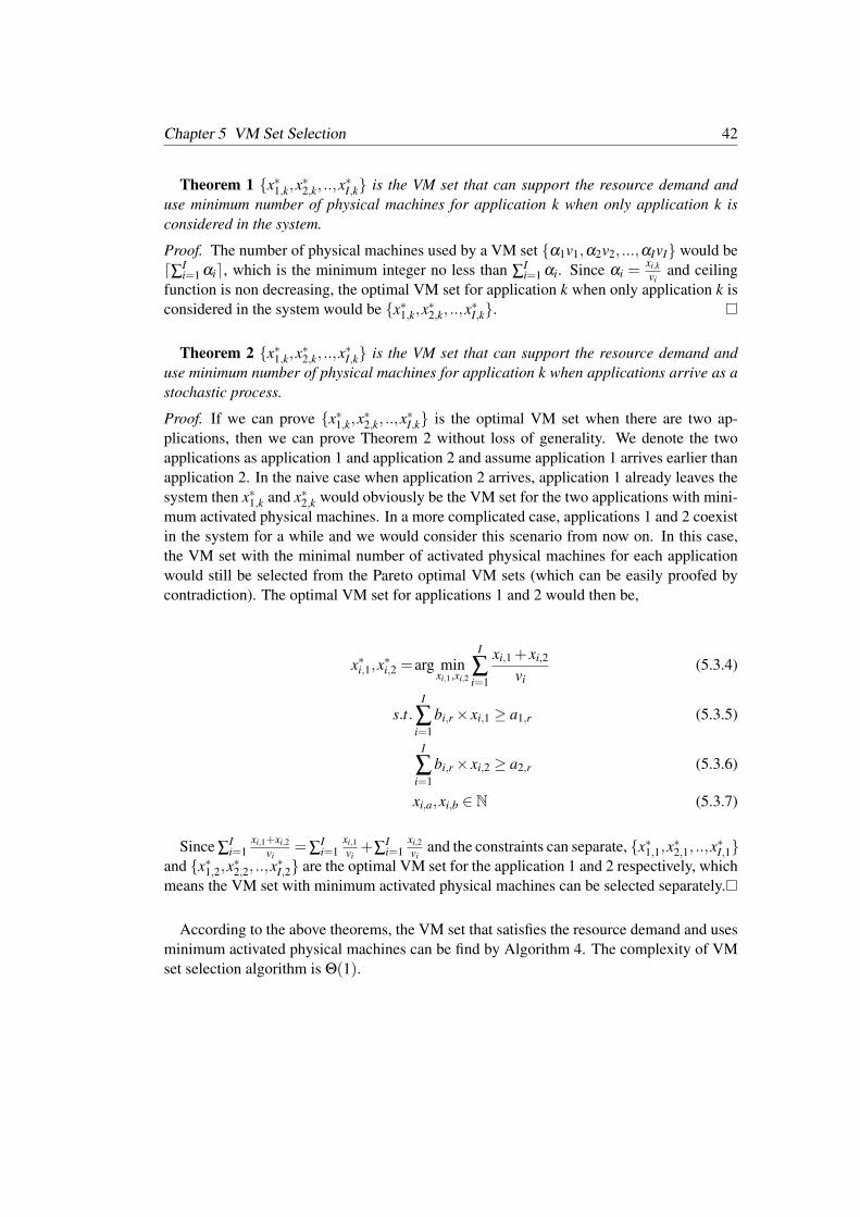
Chapter 5 VM Set Selection 42
Theorem 1 {x∗1,k,x∗2,k, ..,x∗I,k} is the VM set that can support the resource demand anduse minimum number of physical machines for application k when only application k isconsidered in the system.
Proof. The number of physical machines used by a VM set {α1v1,α2v2, ...,αIvI} would bed∑I
i=1 αie, which is the minimum integer no less than ∑Ii=1 αi. Since αi =
xi,kvi
and ceilingfunction is non decreasing, the optimal VM set for application k when only application k isconsidered in the system would be {x∗1,k,x∗2,k, ..,x∗I,k}.
Theorem 2 {x∗1,k,x∗2,k, ..,x∗I,k} is the VM set that can support the resource demand anduse minimum number of physical machines for application k when applications arrive as astochastic process.
Proof. If we can prove {x∗1,k,x∗2,k, ..,x∗I,k} is the optimal VM set when there are two ap-plications, then we can prove Theorem 2 without loss of generality. We denote the twoapplications as application 1 and application 2 and assume application 1 arrives earlier thanapplication 2. In the naive case when application 2 arrives, application 1 already leaves thesystem then x∗1,k and x∗2,k would obviously be the VM set for the two applications with mini-mum activated physical machines. In a more complicated case, applications 1 and 2 coexistin the system for a while and we would consider this scenario from now on. In this case,the VM set with the minimal number of activated physical machines for each applicationwould still be selected from the Pareto optimal VM sets (which can be easily proofed bycontradiction). The optimal VM set for applications 1 and 2 would then be,
x∗i,1,x∗i,2 =arg min
xi,1,xi,2
I
∑i=1
xi,1 + xi,2
vi(5.3.4)
s.t.I
∑i=1
bi,r× xi,1 ≥ a1,r (5.3.5)
I
∑i=1
bi,r× xi,2 ≥ a2,r (5.3.6)
xi,a,xi,b ∈ N (5.3.7)
Since ∑Ii=1
xi,1+xi,2vi
=∑Ii=1
xi,1vi+∑
Ii=1
xi,2vi
and the constraints can separate, {x∗1,1,x∗2,1, ..,x∗I,1}and {x∗1,2,x∗2,2, ..,x∗I,2} are the optimal VM set for the application 1 and 2 respectively, whichmeans the VM set with minimum activated physical machines can be selected separately.
According to the above theorems, the VM set that satisfies the resource demand and usesminimum activated physical machines can be find by Algorithm 4. The complexity of VMset selection algorithm is Θ(1).
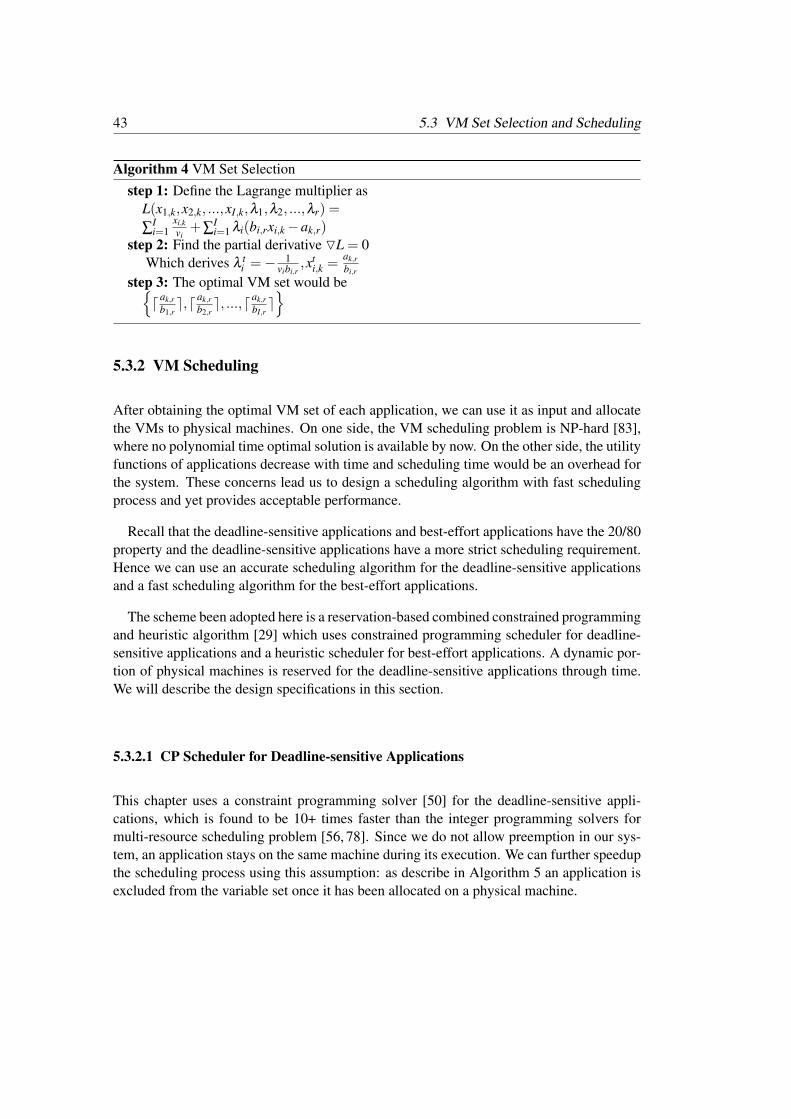
43 5.3 VM Set Selection and Scheduling
Algorithm 4 VM Set Selectionstep 1: Define the Lagrange multiplier as
L(x1,k,x2,k, ...,xI,k,λ1,λ2, ...,λr) =
∑Ii=1
xi,kvi+∑
Ii=1 λi(bi,rxi,k−ak,r)
step 2: Find the partial derivative OL = 0Which derives λ t
i =− 1vibi,r
,xti,k =
ak,rbi,r
step 3: The optimal VM set would be{d ak,r
b1,re,d ak,r
b2,re, ...,dak,r
bI,re}
5.3.2 VM Scheduling
After obtaining the optimal VM set of each application, we can use it as input and allocatethe VMs to physical machines. On one side, the VM scheduling problem is NP-hard [83],where no polynomial time optimal solution is available by now. On the other side, the utilityfunctions of applications decrease with time and scheduling time would be an overhead forthe system. These concerns lead us to design a scheduling algorithm with fast schedulingprocess and yet provides acceptable performance.
Recall that the deadline-sensitive applications and best-effort applications have the 20/80property and the deadline-sensitive applications have a more strict scheduling requirement.Hence we can use an accurate scheduling algorithm for the deadline-sensitive applicationsand a fast scheduling algorithm for the best-effort applications.
The scheme been adopted here is a reservation-based combined constrained programmingand heuristic algorithm [29] which uses constrained programming scheduler for deadline-sensitive applications and a heuristic scheduler for best-effort applications. A dynamic por-tion of physical machines is reserved for the deadline-sensitive applications through time.We will describe the design specifications in this section.
5.3.2.1 CP Scheduler for Deadline-sensitive Applications
This chapter uses a constraint programming solver [50] for the deadline-sensitive appli-cations, which is found to be 10+ times faster than the integer programming solvers formulti-resource scheduling problem [56, 78]. Since we do not allow preemption in our sys-tem, an application stays on the same machine during its execution. We can further speedupthe scheduling process using this assumption: as describe in Algorithm 5 an application isexcluded from the variable set once it has been allocated on a physical machine.
Chapter 5 VM Set Selection 44
5.3.2.2 Heuristic Scheduler for Best-effort Applications
This chapter uses maximum residue as the heuristic scheduler for best-effort application-s. Let’s define the maximum residue scheduler as selecting the physical machine m thatsatisfies the following expression,
argmaxm
R
∑r=1
[lm,r(bi,r
I
∑i
xli,k)] (5.3.8)
where lm,r is the remaining number of type r resource (CPU, memory, storage, etc.) thatcan be hold on physical machine m. xl
i,k is the remaining number of type i VM that haven’tbeen allocated of application k. The heuristic uses dot product to capture the similaritybetween the remaining VM capacity vector of the physical machine and the remaining VMdemand vector of the application. The VMs of an application is assigned to the physicalmachine with a residual capacity that is closest to the application’s remaining VM demand.
The combined constraint programming and the heuristic scheduling algorithms are p-resented in Algorithm 5 and Algorithm 6. To schedule pending jobs, we adopt a basicdeadline-based approach as in Algorithm 7.
Algorithm 5 Combined CP and Heuristic Algorithm
1: When {application k arrives}2: if k is deadline sensitive then3: Heuristic scheduler(k); assign k to an unreserved machine4: else5: CP scheduler(); assign a reserved machine to application k6: if CP failed to assign a reserved machine to k then7: Heuristic scheduler(k); assign k to an unreserved machine8: end if9: end if
10: When {an application k running on machine m finishes}11: Release machine m resources for k12: Schedule a queued job(m)
5.3.2.3 Cluster Reservation for Deadline-sensitive Applications
To better guarantee the deadline requirements for deadline-sensitive applications, this workreserves and dedicates part of the physical machines to accommodate them. When a
45 5.4 Evaluation
Algorithm 6 Heuristic scheduler(k)1: Symbols: k – job to be scheduled2: for Machine m ∈ Unreserved cluster do3: Find min
{mrmk
+ crck
}mr ≥ mk,cr ≥ ck
4: end for5: Assign application k to machine m6: if No unreserved machine available then7: Insert application k to the deadline-ordered queue Q8: end if
Algorithm 7 Schedule a queued job(m)
1: Symbols: m – available machine2: for Application k ∈ job queue Q do3: if Capacity(m)≥ Demand(k) then4: Assign application k to machine m return5: end if6: end for
deadline-sensitive application arrives, it is scheduled (using CP) to one of the reserved ma-chines if there are any left. If no reserved machines is available, it will be scheduled toan unreserved machine using the heuristic algorithm. We use Algorithm 8 to dynamicallydetermine the reservation threshold. The more physical machines are reserved, the higherprobability that a best-effort application will get rejected. On the other side, more physi-cal machines are provided for general use, more deadline-sensitive applications would bescheduled with the less accurate heuristic scheduler. An appropriate reservation thresholdis important to maintain a high utilization rate for the cluster.
5.4 Evaluation
This work evaluates the VM selection and scheduling algorithm in this section using trace-driven simulations. Google Cluster Trace [49, 59] is a public cloud trace from a heteroge-nous workload cloud with around 12,000 machines for a month long period. This work usesGoogle Cluster Trace since it contains both resource demand trace from each applicationand resource usage trace from the physical machines. Resource demand and usage are nor-malized to the largest capacity of the resource on any machine in the trace (which is 1.0).The resource demand trace contains 500 files of application resource demands (in termsof CPU, memory, storage), each with around 5000 applications. Note that an applicationusually contains multiple tasks and each task has a resource demand. However, in this work
Chapter 5 VM Set Selection 46
Algorithm 8 Reservation Threshold(k)1: Symbols: θ – current reservation threshold, ε – adjustment threshold, θ0 – initial
threshold get by tuning, η – adjustment factor get by tuning, qd ,qb – accumulatedweighted resource demand for deadline-sensitive and best-effort applications respec-tively, qk – weighted resource demand of application k
2: When {application k arrives}3: if k is deadline sensitive then4: qd ← qd +qk5: else6: qb← qb +qk7: end if8: if qd
qb< θ0− ε then
9: θ ← θ − ηqkqb
10: else if qdqb
> θ0 + ε then11: θ ← θ + ηqk
qb12: end if
we do not dive into the granularity of tasks and will sum up the resource demand of thetasks into the resource demand of an application. Each application has a field indicating itspriority in terms of high, middle and low. We define the application with high priority asdeadline-sensitive applications and the rest as best-effort applications. Since the trace does-n’t have a deadline field for the applications, we add a deadline for the deadline-sensitiveapplications by ourselves. We first add the deadline as 10% of an application’s duration,and will vary the deadlines and see their effects in later evaluations. We would also varythe utility functions for best-effort application to see their effects in the following part. Weassume 6 primary VM instances listed in Table 5.2. The configurations of the VMs is pro-portional to the VM instances provided by [45]. We will use part of these VM settings inour later simulation. The constraint [57] of the Gecode scheduler been used is the “cumu-latives” constraint provided by the multi-resource scheduling package [50]. The simulationis done on a workstation with quad-core 2.0GHz processor and 16GB RAM.
5.4.1 VM Set Selection
We compare our VM set selection scheme with the resource selection specified in [71] andthe random selection approach (from the Pareto optimal VM sets). The number of physicalmachines used by the three approaches is shown in Fig. 5.1.
As can be seen from the figures that the greedy-optimal VM set selection algorithm will
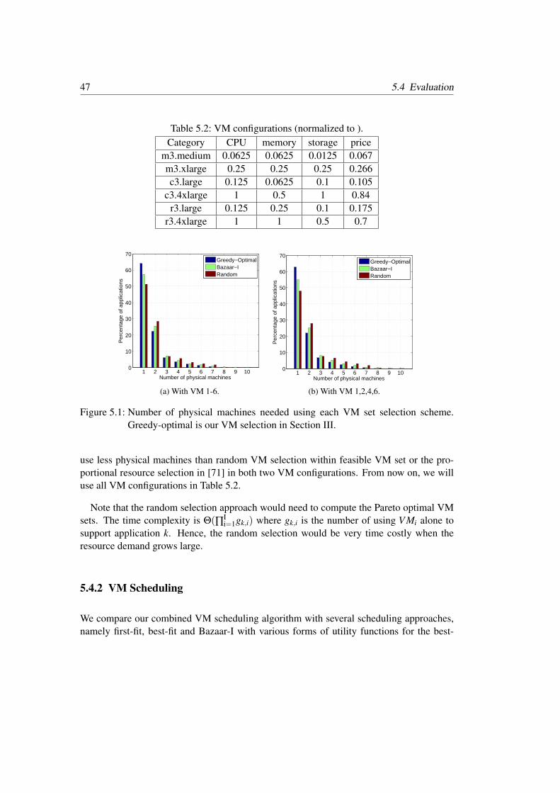
47 5.4 Evaluation
Table 5.2: VM configurations (normalized to ).Category CPU memory storage price
m3.medium 0.0625 0.0625 0.0125 0.067m3.xlarge 0.25 0.25 0.25 0.266c3.large 0.125 0.0625 0.1 0.105
c3.4xlarge 1 0.5 1 0.84r3.large 0.125 0.25 0.1 0.175
r3.4xlarge 1 1 0.5 0.7
1 2 3 4 5 6 7 8 9 100
10
20
30
40
50
60
70
Number of physical machines
Per
cent
age
of a
pplic
atio
ns
Greedy−OptimalBazaar−IRandom
(a) With VM 1-6.
1 2 3 4 5 6 7 8 9 100
10
20
30
40
50
60
70
Number of physical machines
Per
cent
age
of a
pplic
atio
ns
Greedy−OptimalBazaar−IRandom
(b) With VM 1,2,4,6.
Figure 5.1: Number of physical machines needed using each VM set selection scheme.Greedy-optimal is our VM selection in Section III.
use less physical machines than random VM selection within feasible VM set or the pro-portional resource selection in [71] in both two VM configurations. From now on, we willuse all VM configurations in Table 5.2.
Note that the random selection approach would need to compute the Pareto optimal VMsets. The time complexity is Θ(∏I
i=1gk,i) where gk,i is the number of using V Mi alone tosupport application k. Hence, the random selection would be very time costly when theresource demand grows large.
5.4.2 VM Scheduling
We compare our combined VM scheduling algorithm with several scheduling approaches,namely first-fit, best-fit and Bazaar-I with various forms of utility functions for the best-
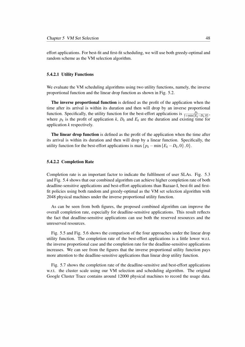
Chapter 5 VM Set Selection 48
effort applications. For best-fit and first-fit scheduling, we will use both greedy-optimal andrandom scheme as the VM selection algorithm.
5.4.2.1 Utility Functions
We evaluate the VM scheduling algorithms using two utility functions, namely, the inverseproportional function and the linear drop function as shown in Fig. 5.2.
The inverse proportional function is defined as the profit of the application when thetime after its arrival is within its duration and then will drop by an inverse proportionalfunction. Specifically, the utility function for the best-effort applications is pk
1+min{Ek−Dk,0} ,where pk is the profit of application k, Dk and Ek are the duration and existing time forapplication k respectively.
The linear drop function is defined as the profit of the application when the time afterits arrival is within its duration and then will drop by a linear function. Specifically, theutility function for the best-effort applications is max{pk−min{Ek−Dk,0} ,0}.
5.4.2.2 Completion Rate
Completion rate is an important factor to indicate the fulfilment of user SLAs. Fig. 5.3and Fig. 5.4 shows that our combined algorithm can achieve higher completion rate of bothdeadline-sensitive applications and best-effort applications than Bazaar-I, best-fit and first-fit policies using both random and greedy-optimal as the VM set selection algorithm with2048 physical machines under the inverse proportional utility function.
As can be seen from both figures, the proposed combined algorithm can improve theoverall completion rate, especially for deadline-sensitive applications. This result reflectsthe fact that deadline-sensitive applications can use both the reserved resources and theunreserved resources.
Fig. 5.5 and Fig. 5.6 shows the comparison of the four approaches under the linear droputility function. The completion rate of the best-effort applications is a little lower w.r.t.the inverse proportional case and the completion rate for the deadline-sensitive applicationsincreases. We can see from the figures that the inverse proportional utility function paysmore attention to the deadline-sensitive applications than linear drop utility function.
Fig. 5.7 shows the completion rate of the deadline-sensitive and best-effort applicationsw.r.t. the cluster scale using our VM selection and scheduling algorithm. The originalGoogle Cluster Trace contains around 12000 physical machines to record the usage data.
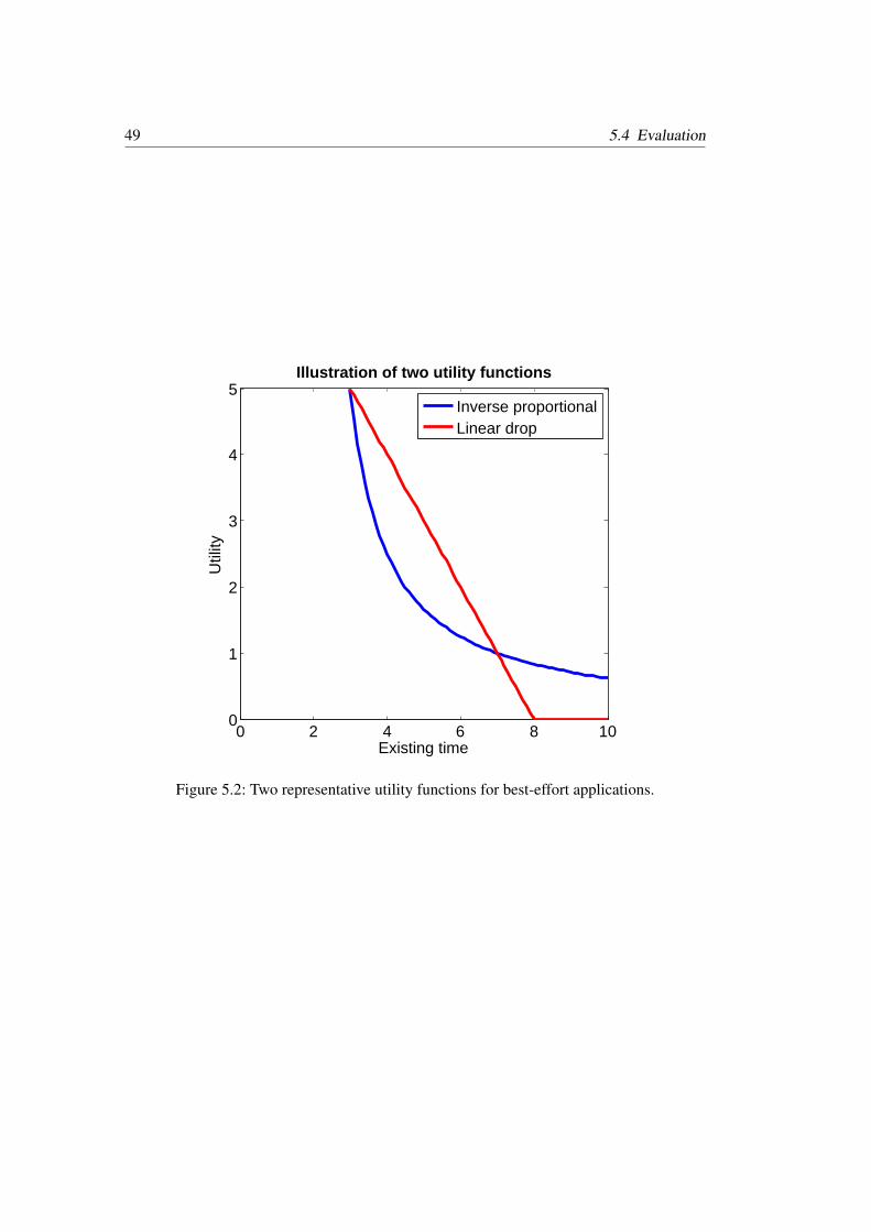
49 5.4 Evaluation
0 2 4 6 8 100
1
2
3
4
5
Existing time
Util
ity
Illustration of two utility functions
Inverse proportionalLinear drop
Figure 5.2: Two representative utility functions for best-effort applications.
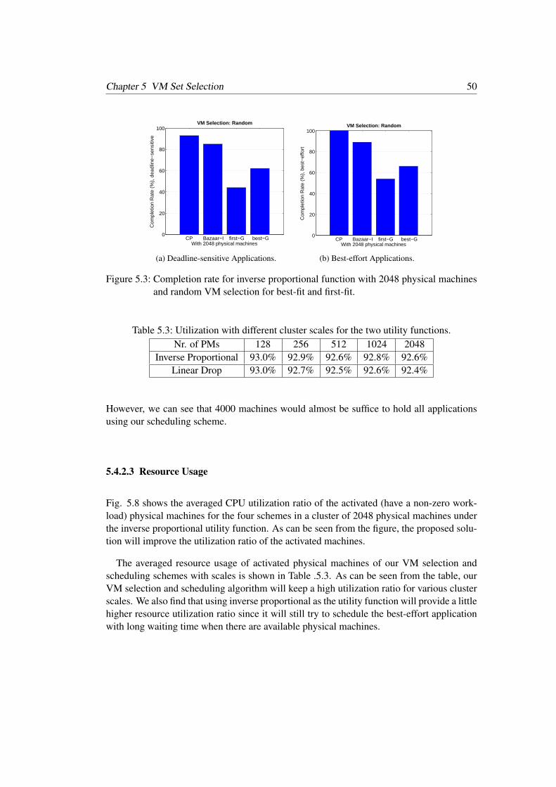
Chapter 5 VM Set Selection 50
CP Bazaar−I first−G best−G0
20
40
60
80
100
Com
plet
ion
Rat
e (%
), d
eadl
ine−
sens
itive
With 2048 physical machines
VM Selection: Random
(a) Deadline-sensitive Applications.
CP Bazaar−I first−G best−G0
20
40
60
80
100
Com
plet
ion
Rat
e (%
), b
est−
effo
rt
With 2048 physical machines
VM Selection: Random
(b) Best-effort Applications.
Figure 5.3: Completion rate for inverse proportional function with 2048 physical machinesand random VM selection for best-fit and first-fit.
Table 5.3: Utilization with different cluster scales for the two utility functions.Nr. of PMs 128 256 512 1024 2048
Inverse Proportional 93.0% 92.9% 92.6% 92.8% 92.6%Linear Drop 93.0% 92.7% 92.5% 92.6% 92.4%
However, we can see that 4000 machines would almost be suffice to hold all applicationsusing our scheduling scheme.
5.4.2.3 Resource Usage
Fig. 5.8 shows the averaged CPU utilization ratio of the activated (have a non-zero work-load) physical machines for the four schemes in a cluster of 2048 physical machines underthe inverse proportional utility function. As can be seen from the figure, the proposed solu-tion will improve the utilization ratio of the activated machines.
The averaged resource usage of activated physical machines of our VM selection andscheduling schemes with scales is shown in Table .5.3. As can be seen from the table, ourVM selection and scheduling algorithm will keep a high utilization ratio for various clusterscales. We also find that using inverse proportional as the utility function will provide a littlehigher resource utilization ratio since it will still try to schedule the best-effort applicationwith long waiting time when there are available physical machines.
51 5.4 Evaluation
CP Bazaar−I first−G best−G0
20
40
60
80
100C
ompl
etio
n R
ate
(%),
dea
dlin
e−se
nsiti
ve
With 2048 physical machines
VM Selection: Greedy−Optimal
(a) Deadline-sensitive Applications.
CP Bazaar−I first−G best−G0
20
40
60
80
100
Com
plet
ion
Rat
e (%
), b
est−
effo
rt
With 2048 physical machines
VM Selection: Greedy−Optimal
(b) Best-effort Applications.
Figure 5.4: Completion rate for inverse proportional function with 2048 physical machinesand greedy-optimal VM selection for best-fit and first-fit.
Table 5.4: Comparison of overall utility with 2048 physical machines and inverse propor-tional utility functions.
Category Inverse Proportional Linear DropCP 1 0.9872
Bazaar-I 0.9144 0.9089first-G 0.5382 0.5426best-G 0.7809 0.7801
5.4.2.4 Overall Utility
The overall utility shows a similar trend with the completion rate. We show our result inTable. 5.4. Note that the overall utility is normalized to our greedy-optimal and combinedconstrained programming solution under inverse proportional utility function for compar-ison purposes. For all four schemes, the overall utility by using inverse proportional andlinear drop are almost the same.
5.4.2.5 Scheduling Speed
Table. 5.5 compares the VM scheduling speed and its accuracy of our combined algorithmwith pure constraint programming on one of the 500 traces.
As can be seen from the table, although CP can achieve higher accuracy, the time com-
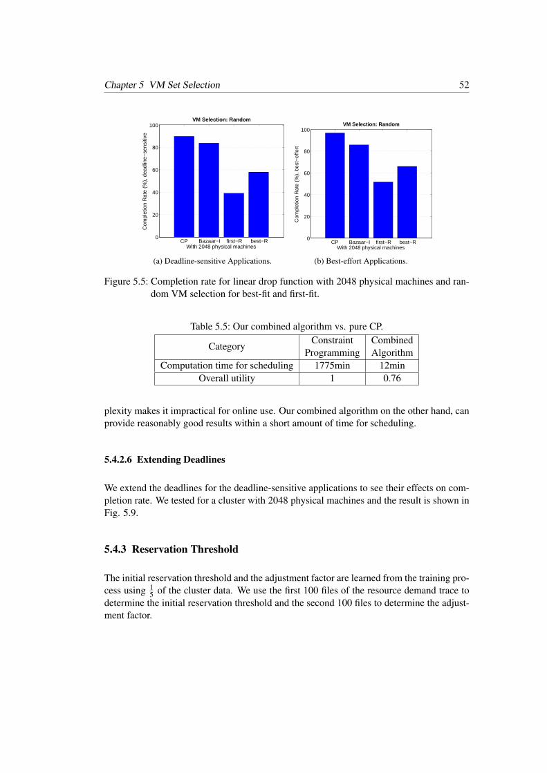
Chapter 5 VM Set Selection 52
CP Bazaar−I first−R best−R0
20
40
60
80
100
Com
plet
ion
Rat
e (%
), d
eadl
ine−
sens
itive
With 2048 physical machines
VM Selection: Random
(a) Deadline-sensitive Applications.
CP Bazaar−I first−R best−R0
20
40
60
80
100
Com
plet
ion
Rat
e (%
), b
est−
effo
rt
With 2048 physical machines
VM Selection: Random
(b) Best-effort Applications.
Figure 5.5: Completion rate for linear drop function with 2048 physical machines and ran-dom VM selection for best-fit and first-fit.
Table 5.5: Our combined algorithm vs. pure CP.
CategoryConstraint
ProgrammingCombinedAlgorithm
Computation time for scheduling 1775min 12minOverall utility 1 0.76
plexity makes it impractical for online use. Our combined algorithm on the other hand, canprovide reasonably good results within a short amount of time for scheduling.
5.4.2.6 Extending Deadlines
We extend the deadlines for the deadline-sensitive applications to see their effects on com-pletion rate. We tested for a cluster with 2048 physical machines and the result is shown inFig. 5.9.
5.4.3 Reservation Threshold
The initial reservation threshold and the adjustment factor are learned from the training pro-cess using 1
5 of the cluster data. We use the first 100 files of the resource demand trace todetermine the initial reservation threshold and the second 100 files to determine the adjust-ment factor.
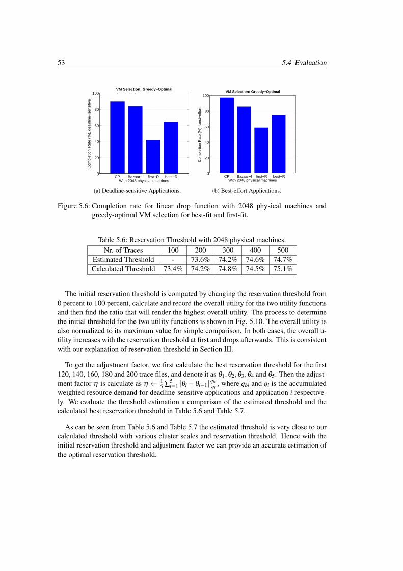
53 5.4 Evaluation
CP Bazaar−I first−R best−R0
20
40
60
80
100C
ompl
etio
n R
ate
(%),
dea
dlin
e−se
nsiti
ve
With 2048 physical machines
VM Selection: Greedy−Optimal
(a) Deadline-sensitive Applications.
CP Bazaar−I first−R best−R0
20
40
60
80
100
Com
plet
ion
Rat
e (%
), b
est−
effo
rt
With 2048 physical machines
VM Selection: Greedy−Optimal
(b) Best-effort Applications.
Figure 5.6: Completion rate for linear drop function with 2048 physical machines andgreedy-optimal VM selection for best-fit and first-fit.
Table 5.6: Reservation Threshold with 2048 physical machines.Nr. of Traces 100 200 300 400 500
Estimated Threshold - 73.6% 74.2% 74.6% 74.7%Calculated Threshold 73.4% 74.2% 74.8% 74.5% 75.1%
The initial reservation threshold is computed by changing the reservation threshold from0 percent to 100 percent, calculate and record the overall utility for the two utility functionsand then find the ratio that will render the highest overall utility. The process to determinethe initial threshold for the two utility functions is shown in Fig. 5.10. The overall utility isalso normalized to its maximum value for simple comparison. In both cases, the overall u-tility increases with the reservation threshold at first and drops afterwards. This is consistentwith our explanation of reservation threshold in Section III.
To get the adjustment factor, we first calculate the best reservation threshold for the first120, 140, 160, 180 and 200 trace files, and denote it as θ1,θ2,θ3,θ4 and θ5. Then the adjust-ment factor η is calculate as η ← 1
5 ∑5i=1 |θi−θi−1|qbi
qi, where qbi and qi is the accumulated
weighted resource demand for deadline-sensitive applications and application i respective-ly. We evaluate the threshold estimation a comparison of the estimated threshold and thecalculated best reservation threshold in Table 5.6 and Table 5.7.
As can be seen from Table 5.6 and Table 5.7 the estimated threshold is very close to ourcalculated threshold with various cluster scales and reservation threshold. Hence with theinitial reservation threshold and adjustment factor we can provide an accurate estimation ofthe optimal reservation threshold.

Chapter 5 VM Set Selection 54
102
103
104
0
20
40
60
80
100
Number of physical machines in the Datacenter
Com
plet
ion
Rat
e (%
)
Deadline−sensitiveBest−effort
Figure 5.7: Completion rate w.r.t. different cluster scales under inverse proportional utilityfunctions.
0 200 400 600 800 1000 1200 140020
30
40
50
60
70
80
90
100
Time(s)
Util
izat
ion
(%)
CPBazaar−Ifirst−Gbest−G
Figure 5.8: CPU utilization ratio with 2048 under inverse proportional utility function.
Table 5.7: Reservation Threshold with 1024 physical machines.Nr. of Traces 100 200 300 400 500
Estimated Threshold - 79.8% 79.5% 80.9% 81.0%Calculated Threshold 80.2% 79.3% 79.8% 81.5% 81.1%
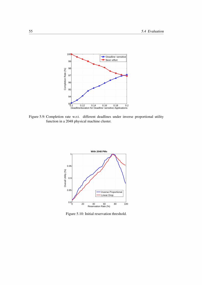
55 5.4 Evaluation
0.1 0.12 0.14 0.16 0.18 0.293
94
95
96
97
98
99
100
Deadline/duration for Deadline−sensitive Applications
Com
plet
ion
Rat
e (%
)
Deadline−sensitiveBest−effort
Figure 5.9: Completion rate w.r.t. different deadlines under inverse proportional utilityfunction in a 2048 physical machine cluster.
0 20 40 60 80 1000.8
0.85
0.9
0.95
1
Reservation Rate (%)
Ove
rall
Util
ity (
%)
With 2048 PMs
Inverse ProportionalLinear Drop
Figure 5.10: Initial reservation threshold.
Chapter 5 VM Set Selection 56
The adjustment threshold ε will affect the stability of the system in terms of adjustmentfrequency. If ε is too small there will be frequent changes between consecutive schedulingdecisions; on the other hand, if ε is too large, the estimated threshold will depart from itstrue value. In this paper, we define the adjustment threshold to be 0.01.
A number of existing works study the VM scheduling problem in cloud environment.The basic VM scheduling problem is related to the multi-dimensional bin packing prob-lems. The primary goal is to use a minimal number of bins to hold all the incoming itemswith jobs arrive and leave in a stochastic manner. The VM scheduling with random arriveand departure time is NP-hard that has no polynomial time optimal solution by now [86]. Asummary of heuristics of the multi-dimensional stochastic bin packing problems can be findin [75]. [72] addresses a joint routing and VM placement problem which extends the binpacking constraints to account for the communication between VMs. [55] gives a good dis-cussion of recent multi-dimensional bin packing problem for theoretical references. How-ever, the stochastic bin packing problem only considers the scheduling from VM to physicalmachines.
There are also literature works address the dynamic VM scheduling problem in a practi-cal way. Yanagisawa et al. [94] proposed an allocation scheme that assigns VMs to phys-ical machines based on the fluctuated CPU demand using mixed integer programming.They partitioned the time-horizon into intervals and allocate the resource periodically toreduce the scheduling time. [29] proposed the combined constraint programming approachfor VM scheduling with fixed deadlines for each applications. [73] considers maximizingthe throughput of a queueing system with a finite number of servers in asymptotic way.The problem with these three approaches is they only consider the VM scheduling prob-lem however there exists multiple feasible VM sets. Jalaparti et al. [71] proposed the ideaof user-oriented resource provisioning. They designed an online scheduler that allows thecloud provider to choose among feasible VM sets to improve the utilization for MapReducejobs. Wieder et al. [85] also aims to select the appropriate VM set for MapReduce jobs, sothat users can specify their goals, such as minimizing monetary cost or completion time.The problem with these two approaches is that they use a heuristic VM set selection algo-rithms, hence would use more physical machines compared to the optimal solution. Whenthe system is overloaded, this would cause low completion rate of the applications. [70]proposed a deadline-aware VM allocation scheme modeling job utilities as a function ofcompletion time. The scheme aims to maximize the minimum utility across all jobs whilethe utilization and profit of the cloud provider is not considered.
In contrast to these works, our work not only allows users to specify their SLA require-ment but also allow various SLAs according to the applications’ characteristics. To the bestof our knowledge, we are also the first to propose the optimal VM set selection algorithmwhich minimizes the number of physical machines for each application.
57 5.5 Chapter Summary
5.5 Chapter Summary
This chapter demonstrates that multiple VM sets can satisfy the application’s resource de-mand and the cloud provider could leverage this property to improve its resource utiliza-tion rate and without violating the applications’ SLAs. We propose a VM set selectionand scheduling approach using combined constraint programming and reservation-basedscheme. We dynamically determine the reservation threshold for deadline-sensitive appli-cations.
Future work includes refining our model to account for the energy consumption for pro-viding datacenter services. The energy consumption for the commodity physical machinesis not proportional to its workload, and the higher the utilization the more energy efficientit would be. Hence, our goal to improve the utilization is consistent with saving energy.Another issue is to incorporate the networking cost between VMs of the same applicationto the VM scheduling problem. The problem could also be modeled into the mixed integerprogramming form. The difficulty lies in transforming the new model into the constraintsprovided by the CP solver.

Chapter6Mobile Cloud Resource Scheduling
Leveraging remote computing resources to execute part of the computation workload frommobile device could improve its performance (in terms of time and scope of applications)and battery life. The underlying rationale is that the speedup by using more powerful remotecomputation resources could potentially overcome the communication delay and schedulingtime overhead. The goal of the scheduler is to improve the performance and battery life ofmobile devices while at the same time maximizing the cloud provider’s profit. There aretwo aspects of mobile cloud resource scheduling problem.
1. Online code partition and offloading. Not all parts of the mobile application shouldrun on the cloud side. Some parts of the application are unremoteable and could onlyrun on the mobile side (such as user interactive components, sensor related compo-nents, etc.). The partition decision is also relevant to the current networking status.The scheduler needs to make the partition decision at runtime w.r.t the latency andbandwidth status.
2. Resource scheduling on cloud side. When there are multiple mobile users request-ing the cloud resource at the same time, the cloud resources are shared by the offload-ed mobile application requests. The cloud scheduler also needs to make the resourceallocation decisions among the submitted mobile requests. The cloud side schedulingalso needs to maintain the mobile side SLA and to improve the cloud side utilizationrate.
This chapter presents an efficient code partition algorithm with high partition accuracyand a cloud resource scheduler that can improve the resource utilization. Our design ismotivated by the clustered offloading property of the call graph, which is based on theobservation that when a method is offloaded, the subsequent invocations will be offloadedwith a high chance. Hence, instead of making an offloading decision for each method asin the 0-1 ILP approach, this work proposes a solution that determines the best offloading
Chapter 6 Mobile Cloud Resource Scheduling 60
and integrating points, which are several starting and ending methods pairs that would havea minimal cost if all the execution sequence in between are offloaded. This work proposesa time complexity code partition algorithm using depth-first search (DFS) and a linear timesearching scheme, where is the number of remoteable methods and is the number invokingrelations in the application. This work evaluates the proposed scheme using two mobileapplications, namely face recognition and natural language processing. Experiments resultsshow that the partition algorithm is 2 orders of magnitude speed up for the face recognitionapplication and the natural language processing application than the 0-1 ILP approach withmore than 90% accuracy.
This chapter is based on the work in [89].
61 6.1 Background and Motivation
6.1 Background and Motivation
A new class of cognition augmenting applications for smartphones such as face or objectrecognition, image or video editing, natural language processing and augmented reality isemerging and attracts increasing attention [63, 64, 69]. This kind of applications requirea large amount of computation, storage and energy which cannot be satisfied by off-the-shelf mobile devices [87]. While more sophisticated hardware can be adopted to carry outthese application tasks, its usage will be limited by its size, weight and monetary cost. Analternative way of facilitating augmented cognition applications on mobile devices is toleverage cloud service or nearby infrastructure to support part of the execution. When theconnection quality to the server is good, offloading some execution to the cloud could bebeneficial. Given the ubiquitous deployment of WiFi/3G networks [76, 77], the ongoingdevelopment of 4G systems [77], and the availability of commercial cloud infrastructure,the future of mobile cloud computing is promising.
More and more mobile computing devices are enjoying the advanced services and appli-cations offered by servers and more recently the cloud infrastructure, ranging from text andimage editing, games, to virus detection, natural language processing, or scientific comput-ing. Each of these applications or jobs require different resource demands, and has differentservice level agreement (SLA) requirements in terms of response time or completion time.For example, interactive applications like image editing or voice detection require a tightresponse time, typically a few seconds. Some production jobs, like virus detection may havea more relax SLA requirements, where users may only require an overall completion timedelay. However, in some cases, no specified completion time delay is provided; instead,the main concern is to get the job done within a overall budget. In fact, various literatureshave shown that the workloads in public clouds are quite diverse in terms of priority, SLArequirement, resource requirement, and job duration [53, 74].
To execute the code on mobile device in mobile cloud computing paradigm, the mobiledevice would offload part of the code from remote infrastructure. A key issue here is to de-termine what’s the most energy- and/or time-efficient way of allocating the components ofthe target application given the current network condition and cloud resource usage status,which is also known as the code partition problem [10], [23], [9], [22]. While cloud infras-tructure provides high computation and service capacity, transferring the input and returnstate is time and energy consuming.
In extreme cases, when the wireless connection is too weak or the amount of state neededto be transferred is too big, executing code on cloud can impair the performance and wasteenergy. Hence, before actually running its code on the cloud environment, an offloadingdecision should be made for the components of the target application with regard to thecurrent network condition and device capacities. We follow the mobile cloud system archi-
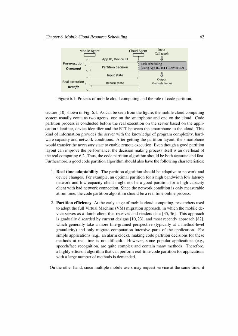
Chapter 6 Mobile Cloud Resource Scheduling 62
Mobile Agent Cloud Agent
App ID, Device ID
Partition decision
Input state
Return state
……
Task scheduling
(using App ID, RTT, Device ID)
Pre-execution
Real execution
Overhead
Benefit
Input
Call graph
Output
Methods layout
Figure 6.1: Process of mobile cloud computing and the role of code partition.
tecture [10] shown in Fig. 6.1. As can be seen from the figure, the mobile cloud computingsystem usually contains two agents, one on the smartphone and one on the cloud. Codepartition process is conducted before the real execution on the server based on the appli-cation identifier, device identifier and the RTT between the smartphone to the cloud. Thiskind of information provides the server with the knowledge of program complexity, hard-ware capacity and network conditions. After getting the partition layout, the smartphonewould transfer the necessary state to enable remote execution. Even though a good partitionlayout can improve the performance, the decision making process itself is an overhead ofthe real computing 6.2. Thus, the code partition algorithm should be both accurate and fast.Furthermore, a good code partition algorithm should also have the following characteristics:
1. Real time adaptability. The partition algorithm should be adaptive to network anddevice changes. For example, an optimal partition for a high bandwidth low latencynetwork and low capacity client might not be a good partition for a high capacityclient with bad network connection. Since the network condition is only measurableat run time, the code partition algorithm should be a real time online process.
2. Partition efficiency. At the early stage of mobile cloud computing, researchers usedto adopt the full Virtual Machine (VM) migration approach, in which the mobile de-vice serves as a dumb client that receives and renders data [35, 36]. This approachis gradually discarded by current designs [10, 23], and most recently approach [82],which generally take a more fine-grained perspective (typically at a method-levelgranularity) and only migrate computation intensive parts of the application. Forsimple applications (e.g., an alarm clock), making code partition decisions for thesemethods at real time is not difficult. However, some popular applications (e.g.,speech/face recognition) are quite complex and contain many methods. Therefore,a highly efficient algorithm that can perform real-time code partition for applicationswith a large number of methods is demanded.
On the other hand, since multiple mobile users may request service at the same time, it
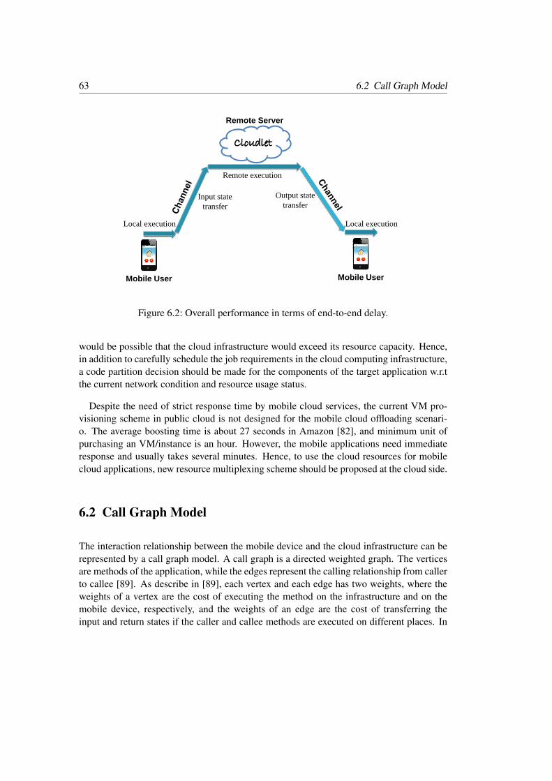
63 6.2 Call Graph Model
Mobile User
Remote execution
Local execution Local execution
Input state
transfer
Output state
transfer
Remote Server
Cloudlet
Mobile User
Figure 6.2: Overall performance in terms of end-to-end delay.
would be possible that the cloud infrastructure would exceed its resource capacity. Hence,in addition to carefully schedule the job requirements in the cloud computing infrastructure,a code partition decision should be made for the components of the target application w.r.tthe current network condition and resource usage status.
Despite the need of strict response time by mobile cloud services, the current VM pro-visioning scheme in public cloud is not designed for the mobile cloud offloading scenari-o. The average boosting time is about 27 seconds in Amazon [82], and minimum unit ofpurchasing an VM/instance is an hour. However, the mobile applications need immediateresponse and usually takes several minutes. Hence, to use the cloud resources for mobilecloud applications, new resource multiplexing scheme should be proposed at the cloud side.
6.2 Call Graph Model
The interaction relationship between the mobile device and the cloud infrastructure can berepresented by a call graph model. A call graph is a directed weighted graph. The verticesare methods of the application, while the edges represent the calling relationship from callerto callee [89]. As describe in [89], each vertex and each edge has two weights, where theweights of a vertex are the cost of executing the method on the infrastructure and on themobile device, respectively, and the weights of an edge are the cost of transferring theinput and return states if the caller and callee methods are executed on different places. In
Chapter 6 Mobile Cloud Resource Scheduling 64
order to correctly execute an application on two separate machines, the system needs totransfer all potential states that could be accessed by the callee or caller. Specifically, theinput state is the input parameter plus the public state which includes the current object’smember variables (including nested member variables), the static classes, and the publicstatic member variables. The return state is the return value plus this public state.
For a given application, the execution cost is affected by input parameters and devicecharacteristics, while the transfer cost is related to the input and network condition. Themetric of cost can either be time or energy consumption. Our partition algorithm is appli-cable to both metrics. However, without loss of generality, we adopt time as the cost metrichereafter because the profiling process does not need any extra device (e.g., a power meter).Given that the computation capacity of the cloud computing infrastructure is stronger thanthat of the mobile device, we assume that the execution time on the infrastructure is smallerthan that on the mobile device. This assumption still holds when using energy consumptionas the cost metric, where only the cost on the mobile device is taken into account.
Not all methods can be executed remotely [9, 10]. For example, methods that interactwith the user interface or access I/O devices and local hardware should not be offloaded(e.g., GPS, accelerator or other sensors). In addition, remote execution might raise securitythreats. In such cases, offloading should be avoided. Automatic classification of suitabilityfor remote execution is possible using static analysis [9].
6.3 Joint Partition and Scheduling Model
The joint code partition and scheduling model is provided in this section. It is worth tomention that the mobile cloud computing model differs from our previous work [88] in thatit satisfies both the cloud computing provider and the mobile user. The goal of the cloudprovider is to maximize its income with fixed number of machines. For the mobile userside, the goal is to meet his or her SLA requirement. To achieve these goals, a new modelis needed to describe the mobile cloud computing system. Similar to public cloud service,to achieve a fair, profitable, and efficient utilization of the available resources at the cloudcomputing infrastructure, we consider the multi-resource pricing policy for mobile cloudcomputing. Since the pricing policy is orthogonal to our resource scheduling problem, weconsider two widely-adopted pricing policies in literature [26, 27, 29, 84]: Market Pricingand Linear Pricing.
Market pricing adopts current cloud operators’s policies [48]. The Google Compute En-gine provides three VM types, namely standard, high memory and high CPU. The config-urations that are not covered by the policy are calculated by interpolation. In this pricing
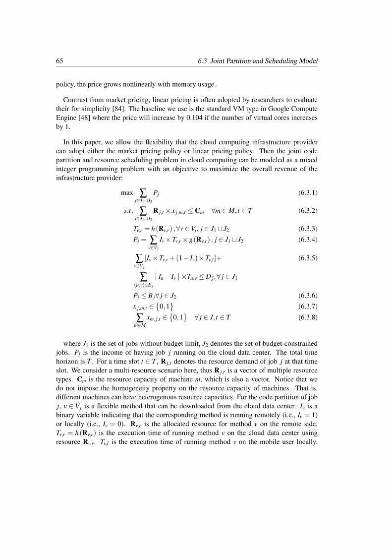
65 6.3 Joint Partition and Scheduling Model
policy, the price grows nonlinearly with memory usage.
Contrast from market pricing, linear pricing is often adopted by researchers to evaluatetheir for simplicity [84]. The baseline we use is the standard VM type in Google ComputeEngine [48] where the price will increase by 0.104 if the number of virtual cores increasesby 1.
In this paper, we allow the flexibility that the cloud computing infrastructure providercan adopt either the market pricing policy or linear pricing policy. Then the joint codepartition and resource scheduling problem in cloud computing can be modeled as a mixedinteger programming problem with an objective to maximize the overall revenue of theinfrastructure provider:
max ∑j∈J1∪J2
Pj (6.3.1)
s.t. ∑j∈J1∪J2
R j,t × x j,m,t ≤ Cm ∀m ∈M, t ∈ T (6.3.2)
Tv,r = h(Rv,r) ,∀v ∈Vi, j ∈ J1∪ J2 (6.3.3)
Pj = ∑v∈Vj
Iv×Tv,r×g(Rv,r) , j ∈ J1∪ J2 (6.3.4)
∑v∈Vj
[Iv×Tv,r +(1− Iv)×Tv,l]+ (6.3.5)
∑(u,v)∈E j
| Iu− Iv | ×Tu,v ≤ D j,∀ j ∈ J1
Pj ≤ B j∀ j ∈ J2 (6.3.6)
x j,m,t ∈{
0,1}
(6.3.7)
∑m∈M
xm, j,t ∈{
0,1}∀ j ∈ J, t ∈ T (6.3.8)
where J1 is the set of jobs without budget limit, J2 denotes the set of budget-constrainedjobs. Pj is the income of having job j running on the cloud data center. The total timehorizon is T . For a time slot t ∈ T , R j,t denotes the resource demand of job j at that timeslot. We consider a multi-resource scenario here, thus R j,t is a vector of multiple resourcetypes. Cm is the resource capacity of machine m, which is also a vector. Notice that wedo not impose the homogeneity property on the resource capacity of machines. That is,different machines can have heterogenous resource capacities. For the code partition of jobj, v ∈ Vj is a flexible method that can be downloaded from the cloud data center. Iv is abinary variable indicating that the corresponding method is running remotely (i.e., Iv = 1)or locally (i.e., Iv = 0). Rv,r is the allocated resource for method v on the remote side,Tv,r = h(Rv,r) is the execution time of running method v on the cloud data center usingresource Rv,r. Tv,l is the execution time of running method v on the mobile user locally.
Chapter 6 Mobile Cloud Resource Scheduling 66
Tu,v is the time overhead for invoking parameter exchange if two interactive methods uand v are not running on the same location. g(Rv,r) is the time-unit pricing function tocharge the method v for utilizing the resource Rv,r from the cloud data center. xm, j,t is abinary scheduling variable, where 1 indicates job j is assigned to machine m at time t and0 otherwise. For jobs with completion time requirements (i.e., D j), the overall executionand data transmission time should not exceed its completion time. For jobs with budgetlimit (i.e., B j), its payment should not exceed its budget. Similar to [88], for any physicalmachine, the resource usage should not exceed its capacities at anytime.
Note that if the workload exceeds the infrastructure’s capacity, not all jobs would get allo-cated in the infrastructure. It is possible that the jobs that do not have a specified completiontime would be postponed. Furthermore, jobs might fail to finish within their specified com-pletion times and violate their SLAs. In this case, they should not contribute to the overallrevenue of the service provider. We assume, jobs can be split such that no job requires morethan 1 physical machine to execute.
As can be seen, this model differs from our [88] work in that it considers the influence ofcode partition towards resource scheduling which is equation 3 to 6.
6.4 Partition and Allocation Algorithm
When all methods are executed on the cloud data center, the joint code partition and re-source scheduling problem will reduce to the SLA-aware multi-resource scheduling prob-lem, which is NP-hard [33]. Hence, the original code partition and resource schedulingproblem is also NP-hard. In mobile cloud computing, no user specified resource demandis available, hence existing resource scheduling algorithms do not apply here. In the mean-while, previous code partition [9, 10] algorithms, including our own approach in [89] aimto minimize the overall time or energy consumption rather than get the specified resourcedemand based on a user provided SLA code partition algorithm needs to be developed.
In this section, we first conservatively estimate the resource demand by leveraging apolynomial time code partition algorithm in our previous work [89]. After obtaining theresource demand, the jobs are allocated to physical machines using a reservation-basedscheduling scheme as describe in our previous work in [88], where the resource demand isused as the input for resource scheduling.
67 6.4 Partition and Allocation Algorithm
6.4.1 Code Partition
In mobile cloud computing, the mobile users do not explicitly specify their resource demandas in normal resource scheduling problems. Instead, an SLA requirement is specified foreach job. To get the user requests allocated, the first thing is to convert the SLA requirementinto specified resource demand for the completion time-aware jobs, we then illustrate howto deduce the resource estimation algorithm for completion time-aware jobs to budget limitjobs.
In the following part, we illustrate the resource estimation scheme for completion time-aware jobs leveraging an optimal polynomial time code partition algorithm. This resourceestimation algorithm differs from our previous work [89] in two ways:
1. the code partition algorithm here is to get a feasible partition and its correspondingresource demand, while in [89], the goal is to get a partition that would minimize theoverall time.
2. the code partition algorithm here works on a general call graph while in our previouswork [89], we need to convert the call graph into a call link.
3. the code partition algorithm provided here is an optimal polynomial time algorithmwhile the algorithm in [89] is a heuristic one.
In the following part, we first proposed a general property on a call graph, so called theminimal download property. Using that property we can obtain a polynomial time codepartition algorithm with the goal to minimize the overall time. To estimate the resourcedemand, we use a binary search approach to conservatively find the resource demand.
6.4.1.1 Minimal Offload Property
We will illustrate the minimal offload property in the following part. Note that in [89], wehave proposed a similar one time offload property. The difference resides in two folds:
1. the minimal offload property works for a general call graph rather than a covertedcall link. Hence, not only the first part of the minimal offload property works on thedifferent context, the second part of the minimal download property never exists inour previous work.
2. the code partition algorithm provided here is an optimal polynomial time algorithmwhile the algorithm in [89] paper is a heuristic one.
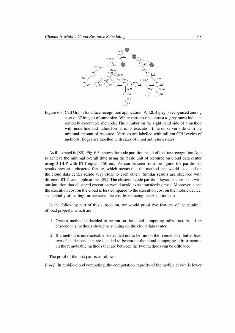
Chapter 6 Mobile Cloud Resource Scheduling 68
Figure 6.3: Call Graph for a face recognition application. A 42kB jpeg is recognised amonga set of 32 images of same size. White vertices (in contrast to grey ones) indicateremotely executable methods; The number on the right hand side of a methodwith underline and italics format is its execution time on server side with theminimal amount of resource. Vertices are labelled with million CPU cycles ofmethods; Edges are labelled with sizes of input ant return states.
As illustrated in [89], Fig. 6.3. shows the code partition result of the face recognition Appto achieve the minimal overall time using the basic unit of resource on cloud data centerusing 0-1ILP with RTT equals 150 ms. As can be seen from the figure, the partitionedresults present a clustered feature, which means that the method that would executed onthe cloud data center reside very close to each other. Similar results are observed withdifferent RTTs and applications [89]. The clustered code partition layout is consistent withour intuition that clustered execution would avoid extra transferring cost. Moreover, sincethe execution cost on the cloud is less compared to the execution cost on the mobile device,sequentially offloading further saves the cost by reducing the execution cost.
In the following part of this subsection, we would proof two features of the minimaloffload property, which are
1. Once a method is decided to be run on the cloud computing infrastructure, all itsdescendants methods should be running on the cloud data center.
2. If a method is unremoteable or decided not to be run on the remote side, but at leasttwo of its descendants are decided to be run on the cloud computing infrastructure,all the remoteable methods that are between the two methods can be offloaded.
The proof of the first part is as follows:
Proof. In mobile cloud computing, the computation capacity of the mobile device is lower
69 6.4 Partition and Allocation Algorithm
compared to the cloud computing server, and this is still true when the basic unit of resourceis allocated on the server side. Hence the execution time of the same method would beless when it runs on the cloud computing than on the mobile device. Let’s consider asimple example with three nodes as illustrated in Fig 6.4, where all the three methods canbe executed both locally and remotely. Assume that the caller of method A will be run on thecloud data center and TA1,TB1,TC1 are the time of transferring the input state, TA2,TB2,TC2are the time of transferring the return state, EA1,EB1,EC1 are the time of executing themethod on the mobile device, while EA2,EB2,EC2 are the time of executing the method onthe cloud data center using the basic resource unit. Since the computation capacity of themobile device is lower compared withe the cloud data center, we have EA1 > EA2,EB1 >EB2,EC1 > EC2. Hence, if method A is to be run on the server, then in the minimal overalltime scheme, method B and C would also be run on the server, since it eliminates the timeof transferring the input and returns state as well as saves time by running the method onthe server.
Another feature of the minimal offload property is that if a method and at least two of itsdescendants are to be run on the server side, all the methods between these two descendantsshould be run on the server. The proof is as follows:
Proof. Let’s consider a general case as shown in fig. 6.5 where all the shown methods areremoteable. Assume method A is decided not to be run on the server side and two of itsdescendants method B and method D are decided to be run on the server side. Since withina single thread, all the methods are run sequentially, which means for any method to run, allits left-hand side brothers are already run. Our claim is that to minimize the overall time anymethod Ci should be run on the server side. We use the contradiction methodology to proveour point. Consider a partition Pk which at least one method Ck is decided to run on themobile device. Compared to the partition where each Ci to be run on the server, Pk woulddefinitely takes more time since it needs both more transferring time and execution time.
6.4.1.2 Minimal Overall Time
In this part, we describe how to find the partition with minimal overall time leveraging theminimal download property we just proved. As shown by the minimal download property,
1. Once a method is decided to be run on the cloud data center, all its descendantsmethods should be running on the cloud data center.
2. Once a method is not decided to be run on the cloud computing infrastructure, itsdescendants should also be run on the server in a clustered manner.
Chapter 6 Mobile Cloud Resource Scheduling 70
We define the minimal remote couple of each method is the starting and ending point oftwo methods that would locally minimize the overall time if the method itself is decided notto be run on the server side. The feasible searching space of each method either its minimalremote couple or itself to be run on the server. In this way, instead of the O(2V ) feasiblesearching space of the 0-1 ILP, the searching space now is O(V ), since when a method isdecided not to be run on the server, the searching space would be reduced to the minimalremote couple.
6.4.1.3 Resource Estimation
Leveraging the minimal offload property, a slow start and binary search algorithm to es-timate the resource demand of the mobile user is provided. The approach we adopt hereis similar to the slow-start algorithm in TCP congestion-avoidance [28]. The idea can beexplained as follows, at first, we allocate the resource on the server side using the basicunit of resource and get the minimal overall time. If this overall time satisfies the user SLArequirement, the corresponding partition would be the one and the resource demand wouldbe the basic resource unit. Else if this overall time exceeds the user specified SLA, doublethe resource allocated on the server side. Repeat this doubling procedure until the overalltime satisfies the user specified SLA. Then use binary search to find the minimal resourcedemand within a range of ε .
The pseudocode code in Algorithm 9 shows how to conservatively find the minimal re-source demand that satisfies the SLA requirements. The first while loop finds a feasiblepartition and its corresponding resource demand that satisfy the user SLA requirement. Thesecond while loop finds the minimal resource demand and its corresponding partition thatsatisfy the user SLA requirement.
6.4.1.4 Resource Estimation for Budget Limit Jobs
Until now we have illustrated how to obtain the resource demand and its correspondingpartition of the completion-time aware jobs. In this following part, we will describe howto leverage the proposed method to obtain the resource demand of the budget limit jobs inAlgorithm 10. Similarly to the resource estimation algorithm of the completion time-awarejobs, this algorithm finds the resource demand that is closest to its budget limitation.
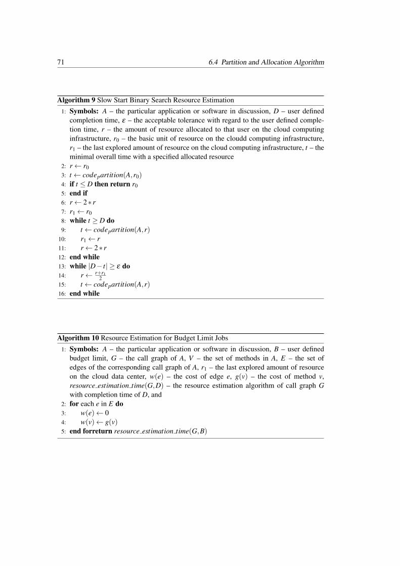
71 6.4 Partition and Allocation Algorithm
Algorithm 9 Slow Start Binary Search Resource Estimation
1: Symbols: A – the particular application or software in discussion, D – user definedcompletion time, ε – the acceptable tolerance with regard to the user defined comple-tion time, r – the amount of resource allocated to that user on the cloud computinginfrastructure, r0 – the basic unit of resource on the cloudd computing infrastructure,r1 – the last explored amount of resource on the cloud computing infrastructure, t – theminimal overall time with a specified allocated resource
2: r← r03: t← codepartition(A,r0)4: if t ≤ D then return r05: end if6: r← 2∗ r7: r1← r08: while t ≥ D do9: t← codepartition(A,r)
10: r1← r11: r← 2∗ r12: end while13: while |D− t| ≥ ε do14: r← r+r1
215: t← codepartition(A,r)16: end while
Algorithm 10 Resource Estimation for Budget Limit Jobs
1: Symbols: A – the particular application or software in discussion, B – user definedbudget limit, G – the call graph of A, V – the set of methods in A, E – the set ofedges of the corresponding call graph of A, r1 – the last explored amount of resourceon the cloud data center, w(e) – the cost of edge e, g(v) – the cost of method v,resource estimation time(G,D) – the resource estimation algorithm of call graph Gwith completion time of D, and
2: for each e in E do3: w(e)← 04: w(v)← g(v)5: end forreturn resource estimation time(G,B)
Chapter 6 Mobile Cloud Resource Scheduling 72
6.5 Evaluation
In this section, we first evaluate the code partition and resource estimation algorithm. Inorder to better understanding our method, this work implements the remote execution plat-form on Android devices and a server. As illustrated in the following, the proposed partitionand estimation algorithm can accurately render a partition result given different user SLA.
Designing an accurate and efficient code partition algorithm for cognition augmentingapplications is challenging. This kind of applications is usually sophisticated and containsa number of remoteable components [10] (i.e., methods that can be offloaded to the cloud).To better understand the characteristics of such applications, we downloaded 3 popularapps (Adobe Photoshop Express [66], Gesture Search [67], and Visidon AppLock [68])from Google Play. We use reverse engineering tools [51, 52] to disassemble the dex filesand find that each of them contains more than 20 remoteable components. We also built twoapplications one face recognition application (The face recognition application is built uponan open source code, which implements the Eigenface face recognition algorithm [43]), andone natural language processing application (The natural language processing applicationis built upon an open source code [44]) from open source code, and find that each of themcontains also more than 15 remoteable components. The time required for solving thecode partition problem by existing works with a 0-1 Integer Linear Programming (0-1 ILP)solver [10,23] is not negligible. For example, in the natural language processing applicationwith 73 components the time needed for partition with 0-1 ILP solver is 7.3s compared to21s time saving.
After getting the resource demand information, the joint code partition and resource al-location problem becomes a pure cluster resource scheduling problem and is solved byour [88] work. Here we just present several results from that work.
6.5.1 Code Partition and Resource Estimation
We implement our code partition and resource estimation algorithm in C on a dual core IntelPentium 2.0GHz processor, 4G RAM desktop. Even though the code partition method itselfis totally different from [89], the input of the code partition algorithm is the same, whichis a call graph which represents the call graph with the following fields: execution time onthe desktop, execution time on the mobile device, a pointer to its first child, a pointer to itsnext sibling, size of the input state to invoke this method, size of the return state, and thenetwork bandwidth. The output of the two algorithms is the partition layout. To obtain theexecution time of a method, we insert a timer in each method and log the execution timeboth on the mobile device and the desktop. The smartphone being used here is the Samsung
73 6.5 Evaluation
Galaxy ACE GT-S5830 with 278 MB RAM and Android 2.3.3 OS. The desktop is equippedwith a dual core Intel Pentium 2.0GHz processor and a 4G RAM. To get the data size, wecurrently use the Sizeof tool developed by Roubtsov [32]. The Sizeof tool calculates anobject’s size in the heap, which is sufficient for obtaining the input of a partition algorithm.In real implementation scenario, we need to actually access the object in heap. This couldbe done via the reflection attribute of the Java language.
As the same with [89], we simulate the transfer time of the input and return state usingthe following rough estimation:
T =state sizebandwidth
(6.5.1)
6.5.1.1 Partition Accuracy
As proved in section 6.4, the proposed code partition algorithm is an optimal polynomialtime algorithm that would find the partition with minimal overall time. The resource es-timation algorithm is also an optimal solution that is bound to find the resource demandclosest to user’s SLA requirement within O(V 2 log2V ) time. Hence, the partition accuracyis evaluated against the heuristic algorithm in our [89] work.
Fig. 6.6 shows the comparison of the optimal minimal time partition with call link basedpartition in terms of overall time. Since the proposed scheme in this paper is an optimalsolution, hence the partition performance is better compared with the heuristic solutionin [89]. Note that the gab between the optimal solution in this paper and the heuristicsolution gets larger when network delay becomes longer, which shows that the performanceof the heuristic algorithm gets worse when network condition gets worse. The optimalsolution enlarges the possibility of using cloud data center, which is the primary gain ofmobile cloud computing.
6.5.1.2 Partition Efficiency
In this part, we will evaluate the code partition speed of the proposed optimal code partitionalgorithm compared with both 0-1 ILP [9, 10] and call link partition [89]. The result isshown in Table 6.1.
As can be seen from the table, the partition speed of the proposed scheme is much higherthan the brutal force 0-1 ILP solver and is quite acceptable with the fact that the computationcapacity of the cloud data center is high.
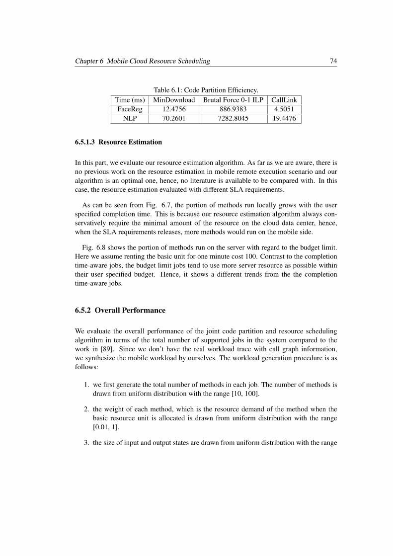
Chapter 6 Mobile Cloud Resource Scheduling 74
Table 6.1: Code Partition Efficiency.Time (ms) MinDownload Brutal Force 0-1 ILP CallLinkFaceReg 12.4756 886.9383 4.5051
NLP 70.2601 7282.8045 19.4476
6.5.1.3 Resource Estimation
In this part, we evaluate our resource estimation algorithm. As far as we are aware, there isno previous work on the resource estimation in mobile remote execution scenario and ouralgorithm is an optimal one, hence, no literature is available to be compared with. In thiscase, the resource estimation evaluated with different SLA requirements.
As can be seen from Fig. 6.7, the portion of methods run locally grows with the userspecified completion time. This is because our resource estimation algorithm always con-servatively require the minimal amount of the resource on the cloud data center, hence,when the SLA requirements releases, more methods would run on the mobile side.
Fig. 6.8 shows the portion of methods run on the server with regard to the budget limit.Here we assume renting the basic unit for one minute cost 100. Contrast to the completiontime-aware jobs, the budget limit jobs tend to use more server resource as possible withintheir user specified budget. Hence, it shows a different trends from the the completiontime-aware jobs.
6.5.2 Overall Performance
We evaluate the overall performance of the joint code partition and resource schedulingalgorithm in terms of the total number of supported jobs in the system compared to thework in [89]. Since we don’t have the real workload trace with call graph information,we synthesize the mobile workload by ourselves. The workload generation procedure is asfollows:
1. we first generate the total number of methods in each job. The number of methods isdrawn from uniform distribution with the range [10, 100].
2. the weight of each method, which is the resource demand of the method when thebasic resource unit is allocated is drawn from uniform distribution with the range[0.01, 1].
3. the size of input and output states are drawn from uniform distribution with the range
75 6.6 Related Work
[100, 1000].
We vary the computation capacity on the server side, hence the allocated resource using[89] would also change correspondingly. The result is shown in Fig. 6.9.
In Fig. 6.9, the server capacity is normalized to the basic resource unit while the Y axisis the job completion rate. As can be seen from the figure, using the joint code partition andresource scheduling algorithm achieve higher job completion rate than the work in [89]. Wealso note that the completion rate using [89] would first increase with the server capacityand then drop. This can be explained by the fact that when more resource are allocatedto a single job, the utilization ratio of the cluster would be low, hence less jobs would beaccommodated.
6.6 Related Work
6.6.1 Mobile Code Partition
Several works are proposed to design systems that combine the computation efforts of mul-tiple machines. Agent Tcl [8] was one such a system that allowed a programmer to easilylet computation jump from one endpoint to another. MAUI [10] enabled automated of-floading and demonstrated that offloading could be an effective tool for performance andenergy gains. However, it still requires annotation of what could be offloaded by develop-ers. CloneCloud [9] to extend this design by using static analysis to automatically decidewhat could be offloaded.
The code partition problem for mobile cloud computing can be categorized by the gran-ularity and partition algorithm been used, current work follows three approaches.
6.6.1.1 Full migration
[35, 36] can also be viewed as an example of the software as a service, which is oftenadopted by early stage research. The inflexibility and coarse granularity of full migrationare the main drawback of this approach.
Chapter 6 Mobile Cloud Resource Scheduling 76
6.6.1.2 Pre-calculated offline partitions
Pre-calculated offline partitions CloneCloud [9] follows this approach. It aims to profileas many execution paths as possible by alternating the inputs and partitions each executionpath under two different network conditions (WiFi and 3G) for time metric or eight states(<CPU, Scr, Net> triples) for energy metric. The smartphone searches for a matchingpartition in the database at run time. However, real network and device conditions cannotbe generalized into fixed amount of states, and using the pre- calculated partitions cannotcover all the offloading scenarios.
6.6.1.3 Making decision at runtime
Examples of this approach are Odessa [22], MAUI [10] and Wishbone [23]. Odessa usesa greedy strategy by estimating whether to offload the current stage would be beneficial.Although the greedy algorithm is fast and can adapt to input and network changes, thedecision is quite unreliable. MAUI and Wishbone formulate the partition problem into a0-1 ILP where each variable is an indicator of whether the corresponding method should beoffloaded. By using the previous profile of last run as an estimator of current run, the wholecall graph can be partitioned with regard to the current network condition. However, thecost of solving the 0-1 ILP is not negligible in terms of time and memory even if it is on theserver side, which is a NP-hard problem and no polynomial solution is available.
The most recent work of mobile cloud resource scheduling are [81, 82]. [81] proposesthe idea to use computation offloading as a service to mobile devices in order to jointlysolve the code partition and resource sharing problem. The problem with this work is thatit doesn’t consider the scheduling time cost. However, as it is shown in the evaluation partof this work, the scheduling actually is critical to the overall performance. [82] presentsa mobile cloud offloading system that considers the end-to-end delay of cloud-enhancedmobile applications. The problem is that it assumes infinite resource on the cloud side.[95] models the code partition and offloading problem into the minimum cut problem andpropose an polynomial time k-cut approximation algorithm. The problem with their workis that there exist some unremoteable components which cannot be represented by the theminimum cut model
6.6.2 Cluster Resource Scheduling
A number of works have been proposed to allocate resource among a fixed number of ma-chines. Yanagisawa et al. [94] presented a resource allocation approach that assigns virtue
77 6.7 Chapter Summary
machines to physical machines based on the fluctuated CPU demand using mixed integerprogramming. To deal with the long processing time of the mixed integer programmingsolver, they developed a technique to partition the time-horizon into intervals and allocatethe resource periodically. The division of intervals makes the scheme insufficient for anonline solution. Niu et al. [34] proposed an iterative resource allocation algorithm with thegoal of maximizing the sum of user utilities minus the cloud operator cost. The convergencetime of their approach is 5 times faster than the gradient methods. Nevertheless, as illus-trated in [24], the speed improvement though significant, still cannot fill up the gap towardsan online scheduling. Jalaparti et al. [71] designed an online scheduling scheme to allowthe cloud operators to choose among all the eligible resource combination to maximize theutilization ratio for MapReduce jobs. Wieder et al. [85] developed a system to select themost appropriate VM for the uses for MapReduce computations, so that users can specifytheir goals, such as minimizing monetary cost or completion time. The problem of [71, 85]lies in that they still assume the fixed and pre-defined VM configurations. As a result, theresource utilization in these approaches is still limited. Our approach differs from theseexisting works in that we exploit the distinct resource requirements for two different typesof jobs and make a tradeoff between them, while able to schedule resources in an onlineand fairly accurate manner. In order to achieve the job specified SLA and to efficientlyuse the resources in the cloud data center, effective resource scheduling mechanism shouldbe employed to carefully assign the incoming jobs onto the appropriate physical machines.Several studies have been proposed to improve the resource efficiency in public cloud datacenter. To handle heterogeneous workloads, Bhattacharya et al. proposed [54] HierarchicalDominant Resource Fairness (H-DRF), which is an online scheduler that achieve high effi-ciency scheduling by equalizing the dominant resource share between each pair of siblingnodes in the hierarchy. [2] proposed an estimation-based opportunistic scheduling algorithmthat can dynamically allocate the resources to each job while maintaining high usage ratio.However, none of these approaches could be directly applied to the mobile cloud comput-ing environment. The problem lies in the interaction between the mobile code partition andthe resource scheduling. The combination of mobile code partition and workload diversitybrings new challenges that do not exist in the traditional resource scheduling setting, andare not fully addressed by the above-mentioned efforts.
6.7 Chapter Summary
Mobile cloud computing is a new computing paradigm that enables mobile users to demandcomputing services from ubiquitous computing infrastructures to access various kinds ofapplications, softwares, and even operation systems. In order to achieve the job specifiedSLA and to efficiently use the resources in the cloud computing infrastructure, effectiveresource scheduling mechanism should be employed to carefully assign the incoming jobs
Chapter 6 Mobile Cloud Resource Scheduling 78
onto the appropriate physical machines. However, no existing approaches could be directlyapplied to the mobile cloud computing environment. The problem lies in the interactionbetween the mobile code partition and the resource scheduling. The combination of mo-bile code partition and workload diversity brings new challenges that do not exist in thetraditional resource scheduling setting, and are not fully addressed by the above-mentionedefforts.
In this paper, we propose a reservation-based code partition and resource scheduling al-gorithm, which is a joint code partition and resource scheduling algorithm. We first estimatethe reservation threshold of the delay-sensitive or completion time-aware jobs, and conser-vatively estimate resource that is available on the cloud computing infrastructure. Givingthe estimated available resource, an linear time code partition algorithm is proposed to getthe minimal completion time. An adjustment of the allocated resource is made for delay-sensitive or completion time-aware jobs if the minimal completion time violates the userspecified SLA.
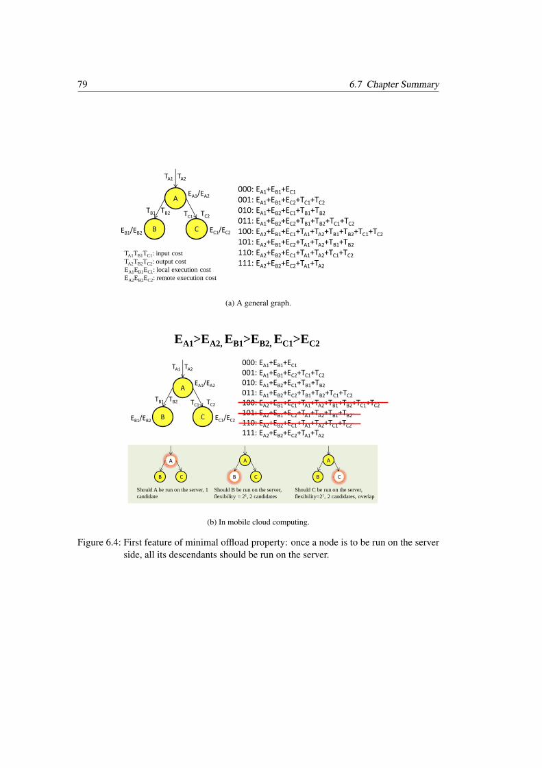
79 6.7 Chapter Summary
1
000: EA1+EB1+EC1 001: EA1+EB1+EC2+TC1+TC2 010: EA1+EB2+EC1+TB1+TB2 011: EA1+EB2+EC2+TB1+TB2+TC1+TC2 100: EA2+EB1+EC1+TA1+TA2+TB1+TB2+TC1+TC2 101: EA2+EB1+EC2+TA1+TA2+TB1+TB2 110: EA2+EB2+EC1+TA1+TA2+TC1+TC2 111: EA2+EB2+EC2+TA1+TA2
A
B C
TA1 TA2
TB1 TB2 TC1 TC2
EA1/EA2
EB1/EB2 EC1/EC2
TA1TB1TC1: input cost
TA2TB2TC2: output cost
EA1EB1EC1: local execution cost
EA2EB2EC2: remote execution cost
(a) A general graph.
EA1>EA2, EB1>EB2, EC1>EC2
000: EA1+EB1+EC1 001: EA1+EB1+EC2+TC1+TC2 010: EA1+EB2+EC1+TB1+TB2 011: EA1+EB2+EC2+TB1+TB2+TC1+TC2 100: EA2+EB1+EC1+TA1+TA2+TB1+TB2+TC1+TC2 101: EA2+EB1+EC2+TA1+TA2+TB1+TB2 110: EA2+EB2+EC1+TA1+TA2+TC1+TC2 111: EA2+EB2+EC2+TA1+TA2
A
B C
TA1 TA2
TB1 TB2 TC1 TC2
EA1/EA2
EB1/EB2 EC1/EC2
A
B C
Should A be run on the server, 1
candidate
Should B be run on the server,
flexibility = 21, 2 candidates
Should C be run on the server,
flexibility=21, 2 candidates, overlap
B C B C
A A
(b) In mobile cloud computing.
Figure 6.4: First feature of minimal offload property: once a node is to be run on the serverside, all its descendants should be run on the server.
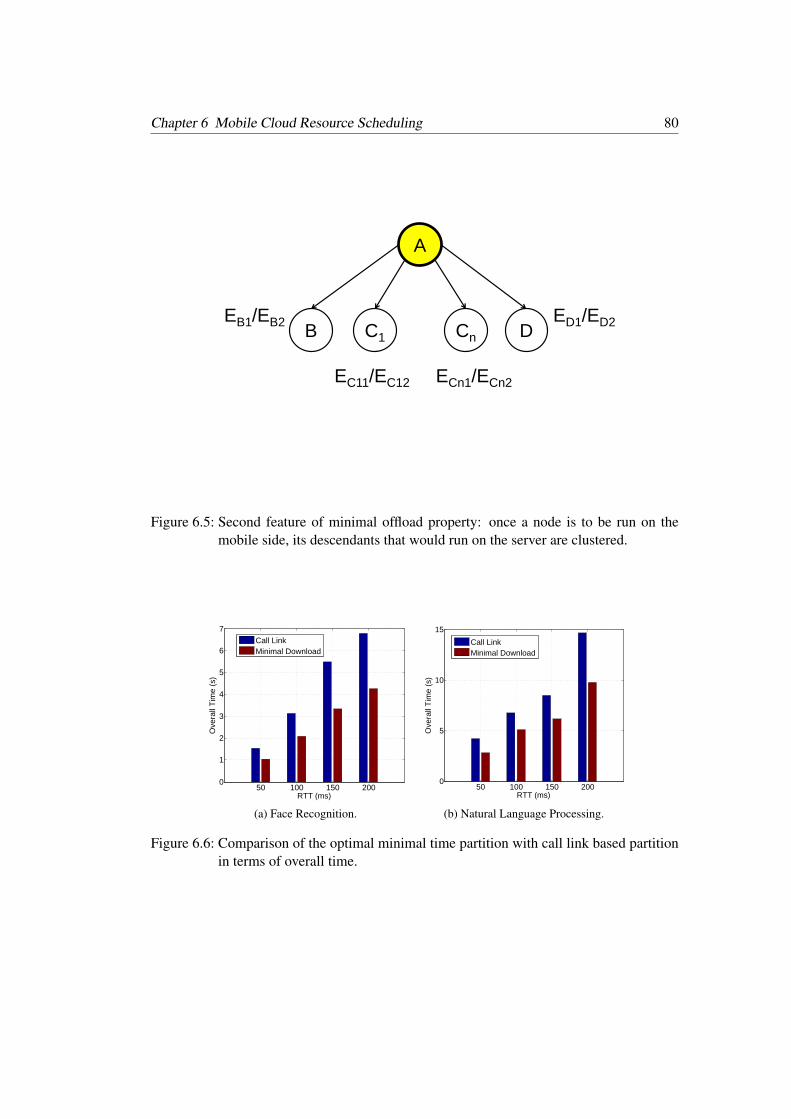
Chapter 6 Mobile Cloud Resource Scheduling 80
A
B C1 Cn DEB1/EB2 ED1/ED2
ECn1/ECn2EC11/EC12
Figure 6.5: Second feature of minimal offload property: once a node is to be run on themobile side, its descendants that would run on the server are clustered.
50 100 150 2000
1
2
3
4
5
6
7
RTT (ms)
Ove
rall
Tim
e (s
)
Call LinkMinimal Download
(a) Face Recognition.
50 100 150 2000
5
10
15
RTT (ms)
Ove
rall
Tim
e (s
)
Call LinkMinimal Download
(b) Natural Language Processing.
Figure 6.6: Comparison of the optimal minimal time partition with call link based partitionin terms of overall time.
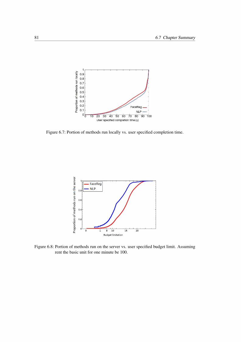
81 6.7 Chapter Summary
Figure 6.7: Portion of methods run locally vs. user specified completion time.
Figure 6.8: Portion of methods run on the server vs. user specified budget limit. Assumingrent the basic unit for one minute be 100.
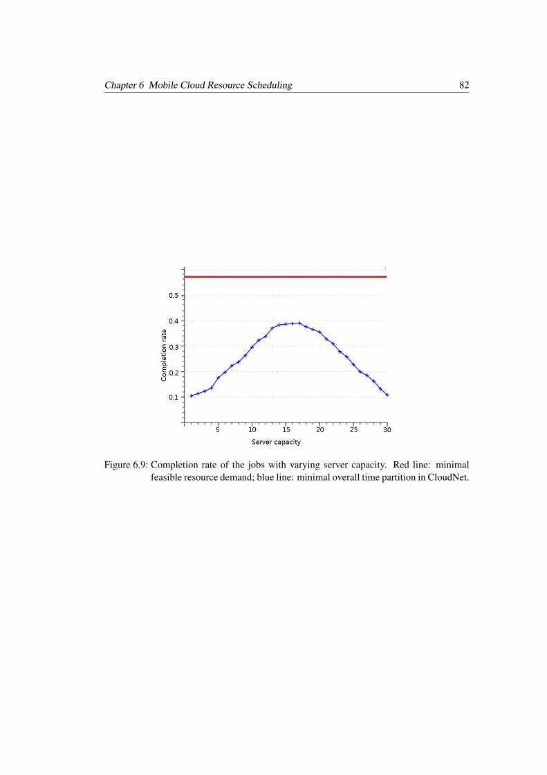
Chapter 6 Mobile Cloud Resource Scheduling 82
Figure 6.9: Completion rate of the jobs with varying server capacity. Red line: minimalfeasible resource demand; blue line: minimal overall time partition in CloudNet.
Chapter7Dissertation Conclusion
This work argues that using finer-grained resource scheduling can benefit both the cloudoperator and the tenants. In addition to evaluation metrics of job completion rate and re-source utilization rate, we also consider the overall revenue of the cloud operator as theoptimization objective which can be seen as a direct reflection of the cloud operator’s in-terest. This also results in meeting the job’s deadline. With objective of maximizing therevenue and taking into account the data center’s capacity constraint, the multi-resourcescheduling problem is modeled as an integer programming problem. However, the tradi-tional integer programming solvers are not applicable here due to the strict requirement foronline resource scheduling to determine the solution quickly and schedule the job so that itcompletes within the deadline.
Using finer-grained resource scheduling can benefit both the cloud operator and the ten-ants. In addition to evaluation metrics of job completion rate and resource utilization rate,we also consider the overall revenue of the cloud operator as the optimization objective.This also results in meeting the job’s deadline. With objective of maximizing the revenueand taking into account the data center’s capacity constraint, the multi-resource schedulingproblem is modeled as an integer programming problem. However, the traditional inte-ger programming solvers are not applicable here due to the strict requirement for onlineresource scheduling to determine the solution quickly and schedule the job so that it com-pletes within the deadline. As summarized in [24], even for a very small scale of jobs andnumber of servers, the time to solve the problem would be unacceptable. For example, inone case tested with 4 machines and 22 jobs, the solution time is 1957.6 seconds on IntelXeon E5420 2.50 GHz computers with 6 MB cache and 6 GB memory.
We analyze the resource demands of jobs from a public cluster trace [49], and find outthat they have a clear relationship to the job duration. The relatively small number of longduration jobs consume the majority of the computing resources. This motivates our ap-proach to tradeoff between scheduling accuracy and scheduling speed: since the few long
Chapter 7 Dissertation Conclusion 84
duration jobs consume most of the resources, a sophisticated scheduling algorithm that canreach an optimal solution is used; on the other hand, for short duration jobs, due to theirlarge number, fast scheduling is important. Therefore, we propose a combined constraintprogramming and heuristic scheduling algorithm. We use constraint programming as thetool to find an optimal scheduling for the long duration jobs. For the jobs with short dura-tions, our experiments show that simple heuristics such as first fit or best fit suffice.
Recent studies like [58,61,70,74,79] show that the applications run on cloud have diverseservice level requirements in terms of throughput, latency, and jitter. These applications canbe coarsely classified into two types: deadline-sensitive applications and best-effort appli-cations [61, 70, 80]. The deadline-sensitive applications often consume large amounts ofresource and have long durations. Furthermore, they are often critical to business, and havestrict deadline requirements. The best-effort applications typically consume less resourceand do not have explicit deadlines. However, finishing the job at an earlier time would im-prove the users’ satisfaction. Based on this observation, we believe that it is highly desirableto design a cloud scheduling system aiming at guaranteeing the deadline requirements of thedeadline-sensitive applications as well as to improve the completion time of the best-effortapplications. Through extensive trace-driven analysis, we find that the number and the re-source consumption of the deadline-sensitive and best-effort applications follows the 80/20principle: While a majority of these applications are best-effort applications, up to 80% ofthe cloud data center resources are consumed by deadline-sensitive applications [61,74,79].We will leverage this property to design an efficient resource scheduling algorithm later.
In this paper, we show that the multiple Pareto optimal VM set property of the appli-cations can be used to improve the overall utilization of the system. We propose a multi-resource scheduler that allocates applications to VM sets and then to physical machines withthe goal to minimize the number of activated physical machines as well as to maximize theoverall utility. The utility function of the deadline-sensitive applications is defined as a 1-0function where the utility would stay the same when it is within its deadline and drop tozero when the it exceeds its deadline. For the best-effort applications, a soft utility func-tion is used where the utility drops gradually [70]. We first provide a greedy yet optimalalgorithm to find the VM set that can minimize the activated physical machines and stillsatisfy the resource requirement. Using the VM sets as input, we model the VM schedulingproblem as an integer programming problem with the goal to improve the overall utilityof all applications. By leveraging the 80/20 property of the deadline-sensitive applicationsand best-effort applications, we propose a combined constraint programming and heuristicalgorithm. We reserve a dynamic number of physical machines for the deadline-sensitiveapplications and use constraint programming to get a more accurate scheduling result. Dueto the huge number and the less resource consumption of the best-effort applications, weuse heuristic scheduling policy to get a fast yet acceptable scheduling result. Trace-drivensimulation shows over 25% improvement of the overall utility compared to best-fit and first-

85
fit using the optimal VM selection algorithm, over 30% improvement compared to best-fitand first-fit using random VM selection scheme and 18% improvement compared to theBazaar-I approach.


Chapter8Bibliography

Bibliography
[1] A. A. Bhattacharya, D. Culler, E. Friedman, A. Ghodsi, S. Shenker, and I. Stoica, Hier-archical Scheduling for Diverse Datacenter Workloads, SoCC, 2013.
[2] E. Boutin, J. Ekanayake, W. Lin, B. Shi, J. Zhou, Z. Qian, M. Wu, and L. Zhou, Apollo:Scalable and Coordinated Scheduling for Cloud-Scale Computing, OSDI, 2014.
[3] C. J. Wong, S. Sen, T. Lan, and M. Chiang. Multi-resourceallocation: Fairness-efficiency tradeoffs in a unifying framework. In INFOCOM, pages 1206–1214, 2012.
[4] A. Ghodsi, V. Sekar, M. Zaharia, and I. Stoica. Multi-resource fair queueing for packetprocessing. In SIGCOMM, 2012.
[5] H. Ying, W. Yang, G. Wang, Wireless Multicast for Mobile Transparent Computing,High Performance Computing and Communications (HPCC), 2013.
[6] W. Liang, Y. Xiong, M. Wu, A Cross Platform Computing Method and Its Applica-tion for Mobile Device in Transparent Computing, High Performance Computing andCommunications (HPCC), 2013.
[7] H. Liu. A Measurement Study of Server Utilization in Public Clouds. Int. Conf. onCloud and Green Computing (CGC), Dec. 2011.
[8] R. S. Gray, Agent Tcl: A flexible and secure mobile-agent system, Technical Report,Dartmouth College Hanover, 1998
[9] B. G. Chun, S. Ihm, P. Maniatis, M. Naik and A. Patti. Cloud: Elastic Execution be-tween Mobile Device and Cloud. EuroSys 2011.
[10] E. Cuervo, A. Balasubramanian, D. Cho, A. Wolman, S. Saroiu, R. Chandra, and P.Bahl, MAUI: Making Smartphones Last Longer with Code Offload, MobiSys 2010.
[11] C. Wang, T. Javidi and George Porter. End-to-End Scheduling for All-Optical DataCenters. INFOCOM 2015.
[12] G. Birkhoff. Tres observaciones sobre el algebra lineal. Univ. Nac. Tucuman Rev. Ser.
Bibliography 90
A5, no. 147-150, 1946.
[13] L. Wang, A. Nappa, J. Caballero, T. Ristenpart and A Akella. WhoWas: A Platformfor Measuring Web Deployments on IaaS Clouds. INFOCOM IMC 2014.
[14] M. Conley, A. Vahdat and G. Porter. Achieving Cost-efficient, Data-intensive Com-puting in the Cloud. ACM SoCC 2015.
[15] E. Walker. Benchmarking Amazon EC2 for high-performance scientific computing.LOGIN, 2008.
[16] P. Mehrotra, J. Djomehri, S. Heistand, R. Hood, H. Jin, A. Lazanoff, S. Saini, andR. Biswas. Performance evaluation of Amazon EC2 for NASA HPC applications. InScienceCloud, 2012.
[17] G. Wang and T. E. Ng. The impact of virtualization on network performance of Ama-zon EC2 data center. IEEE INFOCOM, 2010.
[18] J. Schad, J. Dittrich, and J. Quiane-Ruiz. Runtime measurements in the cloud: Ob-serving, analyzing, and reducing variance. In VLDB, 2010.
[19] F. Chen, M. Kodialam, and T. Lakshman. Joint scheduling of processing and shufflephases in mapreduce systems. IEEE INFOCOM, 2012.
[20] http://www.gecode.org/doc-latest/reference
[21] C. Delimitrou, D. Sanchez, and C. Kozyrakis, Tarcil: Reconciling Scheduling Speedand Quality in Large Shared Clusters, SoCC 2015.
[22] M. R. Ra, A. Sheth, L. Mummert, P. Pillai, D. Wetherall, and R. Govindan. Odessa:Enabling Interactive Perception Applications on Mobile Devices. MobiSys 2011.
[23] R. Newton, S. Toledo, L. Girod, H. Balakrishnan, and S. Madden. Wishbone: Profile-based Partitioning for Sensornet Applications. NSDI 2009.
[24] S. Heinz, J. C. Beck. Solving Resource Allocation/Scheduling Problems with Con-straint Integer Programming. Workshop on Constraint Satisfication Techniques forPlanning and Scheduling Problems, 2011.
[25] M. Mihailescu, Y. M. Teo. Dynamic Resource Pricing on Federated Clouds. CCGrid2010.
[26] L. Popa, G. Kumar, et al. FairCloud: Sharing the Network in Cloud Computing. ACMSIGCOMM 2012.
91 Bibliography
[27] H. Roh, C. Jung, et al. Resource Pricing Game in Geo-distributed Clouds. IEEE IN-FOCOM 2013.
[28] W. Stevens, RFC2001: TCP Slow Start, Congestion Avoidance, Fast Retransmit, andFast Recovery Algorithms, tools.ietf.org/html/rfc2001
[29] H. Zhang, B. Li, H. B. Jiang. A Framework for Truthful Online Auctions in CloudComputing with Heterogeneous User Demands. IEEE INFOCOM 2013.
[30] Y Zheng, N. B. Shroff, R. Srikant and P. Sinha. Exploiting Large System Dynamicsfor Designing Simple Data Center Schedulers. IEEE INFOCOM 2015.
[31] Y. Chen, S. Alspaugh, A. Ganapathi, R. Griffith, R. Katz, Statistical Workload Injectorfor MapReduce(SWIM): https://github.com/SWIMProjectUCB/SWIM/wiki
[32] V. Roubtsov, Sizeof, http://www.javaworld.com/javaworld/ javatips/jw-javatip130.html
[33] M.P.J. Fromherz. Constraint-based scheduling. American Control Conference, 2001.
[34] D. Niu, B. Li. An Efficient Distributed Algorithm for Resource Allocation in Large-Scale Coupled Systems. IEEE INFOCOM 2013.
[35] S. Osman, D. Subhraveti, G. Su, and J. Nieh. The Design and Implementation of Zap:A System for Migrating Computing Environments. OSDI 2002.
[36] M. Satyanarayanan, P. Bahl, R. Caceres, and N. Davies. The Case for VM-basedCloudlets in Mobile Computing. IEEE Pervasive Computing, 8(4), 2009.
[37] A. Wieder, P. Bhatotia, et al. Orchestrating the Deployment of Computations in theCloud with Conductor. USENIX NSDI 2012.
[38] L. E. Dubois, G. Mounie, D. Trystram, Analysis of Scheduling Algorithms with Reser-vations. IEEE IPDPS 2007.
[39] http://aws.amazon.com/solutions/case-studies/netflix/
[40] http://aws.amazon.com/solutions/case-studies/notre-dame/
[41] http://aws.amazon.com/solutions/case-studies/major-league-baseball/
[42] P. Garraghan, P. Townend, J. Xu. An Analysis of the Server Characteristics and Re-source Utilization in Google Cloud. IEEE Int. Conf. on Cloud Engineering, Sep. 2013.
[43] http://darnok.org/programming/face-recognition/
Bibliography 92
[44] http://nlp.stanford.edu/software/index.shtml
[45] http://aws.amazon.com/ec2
[46] http://aws.amazon.com/ec2/instance-types/
[47] https://aws.amazon.com/ec2/purchasing-options/
[48] Google Compute Engine Pricing. https://cloud.google.com/products/compute-engine/
[49] https://code.google.com/p/googleclusterdata/
[50] http://www.gecode.org/
[51] http://code.google.com/p/dex2jar
[52] http://java.decompiler.free.fr/?q=jdgui
[53] Q. Zhang, M. Zhani, R. Boutaba, and J. L. Hellerstein. Dynamic Heterogeneity-awareResource Provisioning in the Cloud. ICDCS 2013.
[54] A. Bhattacharya, D. Culler, E. Friedman, A. Ghodsi, S. Shenker, and I. Stoica. Hierar-chical Scheduling for Diverse Datacenter Workloads. ACM SOCC 2013
[55] N. Bansal, A. Caprara, M. Sviridenko. A New Approximation Method for Set Cover-ing Problems, with Applications to Multidimensional Bin Packing. SIAM J. Comput.,2009, Vol.39, No.4, pp.1256-1278.
[56] R. Bartak. Guide to Constraint Programming.http://kti.ms.mff.cuni.cz/∼bartak/constraints/intro.html
[57] N. Beldiceanu and M. Carlsson. A New Multi-Resource Cumulatives Constraint withNegative Heights. Principles and Practice of Constraint Programming, 2002.
[58] R. Boutaba, L. Cheng and Q. Zhang. On cloud computational models and the hetero-geneity challenge. J. Internet Services and Applications, 3(1):77–86, 2012
[59] C. Reiss and J. Wilkes, Google cluster-usage traces: format + schema, 2011
[60] L. Zhang, C. Wu, Z. Li, C. Guo, M. Chen and F. C.M. Lau. Moving Big Data toThe Cloud: An Online Cost-Minimizing Approach. IEEE Journal on Selected Areas inCommunications (JSAC), 2015.
[61] C. Curino, D. Difallah, C. Douglas, S. Krishnan, R. Ramakrishnan and S. Rao.Reservation-based Scheduling: If You’re Late Don’t Blame Us! ACM SOCC 14.
93 Bibliography
[62] D. Gamarnik. Stochastic Bandwidth Packing Process: Stability Conditions via Lya-punov Function Technique. Queueing Systems, 2004, Vol.48, pp.339-363.
[63] J. Cohen, Embedded speech recognition applications in mobile phones: Status, trends,and challenges, IEEE ICASSP 2008.
[64] Apple Litigation Marks A New Era Of Expectations For Voice Recogni-tion, http://seekingalpha.com/article/432161-apple-litigation-marks-a-new-era-of-expectations-for-voice-recognition, March 2012.
[65] J. C. Mogul and R. R. Kompella. Inferring the Network Latency Requirements ofCloud Tenants. In Proc. of USENIX HotOS, 2015
[66] Adobe Photoshop Express, https://play.google.com/store/apps/details?id=com.adobe.psmobile
[67] Gesture Search, https://play.google.com/store/apps/details?id=com.google.android.apps.gesturesearch
[68] Visidon AppLock, https://play.google.com/store/apps/details?id=visidon.AppLock
[69] G. Hua, Y. Fu, M. Turk, M. Pollefeys, and Z. Zhang, Introduction to the Special Issueon Mobile Vision, International Journal of Computer Vision, vol. 3, pp. 277-279 , 2012.
[70] Z. Huang, B. Balasubramanian, M. Wang, T. Lan, M. Chiang, and D. Tsang, Needfor Speed: CORA Scheduler for Optimizing Completion-Times in the Cloud. IEEEINFOCOM 2015.
[71] V. Jalaparti, H. Ballani, P. Costa, T. Karagiannis, A. Rowstron. Bridging the Tenant-Provider Gap in Cloud Services. ACM SOCC 2012.
[72] J. W. Jiang, T. Lan, S. Ha, M. Chen, and M. Chiang. Joint VM Placement and Routingfor Data Center Traffic Engineering. IEEE INFOCOM 2012.
[73] S. T. Maguluri, R. Srikant, and L. Ying. Stochastic Models of Load Balancing andScheduling in Cloud Computing Clusters. IEEE INFOCOM 2012.
[74] A. Mishra, J. Hellerstein, W. Cirne, and C. Das. Towards characterizing cloud backendworkloads: insights from Google compute clusters. ACM SIGMETRICS 2010.
[75] R. Panigrahy, K. Talwar, L. Uyeda, U. Wieder. Heuristics for Vector Bin Packing. InMSR TR, 2011.
[76] J. Xia, The third-generation-mobile (3G) policy and deployment in China: Currentstatus, challenges, and prospects. Telecommunications Policy, 2011
Bibliography 94
[77] Global mobile statistics 2012 Home: all the latest stats on mobile Web, apps, mar-keting, advertising, subscribers and trends. http://mobithinking.com/mobile-marketing-tools/latest-mobile-stats/
[78] C. L. Pape. Constraint-Based Scheduling: A Tutorial.
[79] C. Reiss, A. Tumanov, G. Ganger, R. Katz, and M. Kozuch. Heterogeneity and Dy-namicity of Clouds at Scale: Google Trace Analysis. ACM SOCC 2012
[80] M. Schwarzkopf, A. Konwinski, M. Malek, and J.Wilkes. Omega: flexible, scalableschedulers for large compute clusters. ACM EuroSys, 2013
[81] C. Shi, K. Habak, P. Pandurangan, M. Ammar, M. Naik, and E. Zegura. COSMOS:computation offloading as a service for mobile devices. ACM MobiHoc, 2014
[82] L. Ravindrantah, J. Padhye, R. Mahajan, and H. Balakrishnan. Timecard: ControllingUser-Perceived Delays in Server-Based Mobile Applications. ACM SOCC 2014.
[83] A. L. Stolyar, Y. Zhong. A large-scale service system with packing constraints: Mini-mizing the number of occupied servers. ACM SIGMETRICS 2013, Pittsburgh, PA, Jun.2013.
[84] M. Mihailescu, Y. M. Teo. Dynamic Resource Pricing on Federated Clouds. CCGrid2010.
[85] A. Wieder, P. Bhatotia, A. Post, and R. Rodrigues, Orchestrating the Deployment ofComputations in the Cloud with Conductor. USENIX NSDI 2012
[86] G. J. Woeginger. There Is No Asymptotic Ptas For Two-Dimensional Vector Packing.In Information Processing Letters, 1997.
[87] T. Park, J. Lee, I. Hwang, C. Yoo, L Nachman, and J. Song, E-Gesture: a collaborativearchitecture for energy-efficient gesture recognition with hand-worn sensor and mobiledevices. SenSys 2011
[88] Y. Zhang, X. Fu, K. K. Ramakrishnan, Fine-Grained Multi-Resource Scheduling inCloud Datacenters, The 20th IEEE International Workshop on Local and MetropolitanArea Networks (LANMAN 2014), invited paper, May 2014.
[89] Y. Zhang, H. Liu, L. Jiao, X. Fu, 1st IEEE International Conference on Cloud Net-working (CloudNet 2012), Paris, France, November 2012.
[90] L. Zheng, C. J-Wong, C. W. Tan, M. Chiang, and X. Wang. How to Bid the Cloud.SIGCOMM 2015.
95 Bibliography
[91] F. R. Dogar, T. Karagiannis, H. Ballani, and A. Rowstron. Decentralized task-awarescheduling for data center networks. ACM SIGCOMM 2014.
[92] N. Jain, I. Menache, J. S. Naor, and Yaniv, J. Near-optimal scheduling mechanisms fordeadline-sensitive jobs in large computing clusters. ACM Trans. on Parallel Computing,2015.
[93] J. Nair, V. G. Subramanian, and A. Wierman. On competitive provisioning of cloudservices. ACM SIGMETRICS 2014.
[94] H. Yanagisawa, T. Osogami, R. Raymond. Dependable Virtual Machine Allocation.IEEE INFOCOM 2013.
[95] Y. H. Kao, B. Krishnamachari, M. R. Ra and F. Bai. Hermes: Latency Optimal TaskAssignment for Resource-constrained Mobile Computing. IEEE INFOCOM 2015.

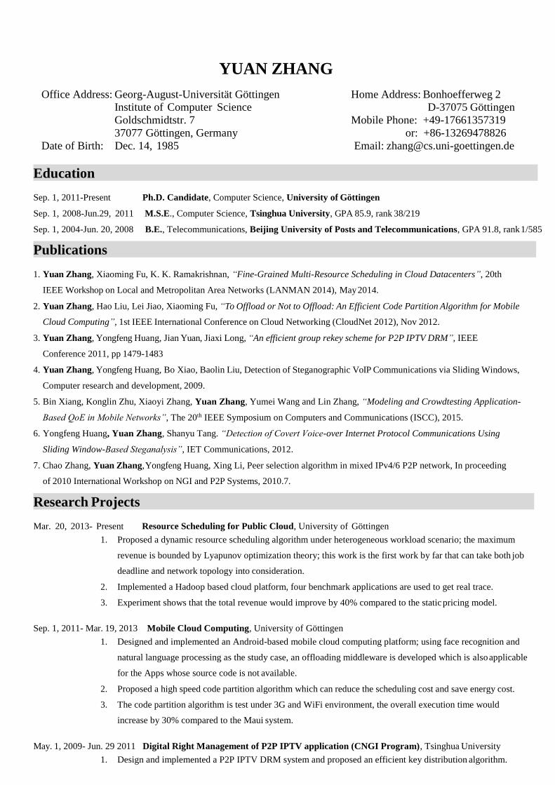
YUAN ZHANG
Office Address: Georg-August-Universität Göttingen Home Address: Bonhoefferweg 2
Institute of Computer Science D-37075 Göttingen
Goldschmidtstr. 7 Mobile Phone: +49-17661357319
37077 Göttingen, Germany or: +86-13269478826
Date of Birth: Dec. 14, 1985 Email: [email protected]
Education
Sep. 1, 2011-Present Ph.D. Candidate, Computer Science, University of Göttingen
Sep. 1, 2008-Jun.29, 2011 M.S.E., Computer Science, Tsinghua University, GPA 85.9, rank 38/219
Sep. 1, 2004-Jun. 20, 2008 B.E., Telecommunications, Beijing University of Posts and Telecommunications, GPA 91.8, rank 1/585
Publications
1. Yuan Zhang, Xiaoming Fu, K. K. Ramakrishnan, “Fine-Grained Multi-Resource Scheduling in Cloud Datacenters”, 20th
IEEE Workshop on Local and Metropolitan Area Networks (LANMAN 2014), May 2014.
2. Yuan Zhang, Hao Liu, Lei Jiao, Xiaoming Fu, “To Offload or Not to Offload: An Efficient Code Partition Algorithm for Mobile
Cloud Computing”, 1st IEEE International Conference on Cloud Networking (CloudNet 2012), Nov 2012.
3. Yuan Zhang, Yongfeng Huang, Jian Yuan, Jiaxi Long, “An efficient group rekey scheme for P2P IPTV DRM”, IEEE
Conference 2011, pp 1479-1483
4. Yuan Zhang, Yongfeng Huang, Bo Xiao, Baolin Liu, Detection of Steganographic VoIP Communications via Sliding Windows,
Computer research and development, 2009.
5. Bin Xiang, Konglin Zhu, Xiaoyi Zhang, Yuan Zhang, Yumei Wang and Lin Zhang, “Modeling and Crowdtesting Application-
Based QoE in Mobile Networks”, The 20th IEEE Symposium on Computers and Communications (ISCC), 2015.
6. Yongfeng Huang, Yuan Zhang, Shanyu Tang. “Detection of Covert Voice-over Internet Protocol Communications Using
Sliding Window-Based Steganalysis”, IET Communications, 2012.
7. Chao Zhang, Yuan Zhang, Yongfeng Huang, Xing Li, Peer selection algorithm in mixed IPv4/6 P2P network, In proceeding
of 2010 International Workshop on NGI and P2P Systems, 2010.7.
Research Projects
Mar. 20, 2013- Present Resource Scheduling for Public Cloud, University of Göttingen
1. Proposed a dynamic resource scheduling algorithm under heterogeneous workload scenario; the maximum
revenue is bounded by Lyapunov optimization theory; this work is the first work by far that can take both job
deadline and network topology into consideration.
2. Implemented a Hadoop based cloud platform, four benchmark applications are used to get real trace.
3. Experiment shows that the total revenue would improve by 40% compared to the static pricing model.
Sep. 1, 2011- Mar. 19, 2013 Mobile Cloud Computing, University of Göttingen
1. Designed and implemented an Android-based mobile cloud computing platform; using face recognition and
natural language processing as the study case, an offloading middleware is developed which is also applicable
for the Apps whose source code is not available.
2. Proposed a high speed code partition algorithm which can reduce the scheduling cost and save energy cost.
3. The code partition algorithm is test under 3G and WiFi environment, the overall execution time would
increase by 30% compared to the Maui system.
May. 1, 2009- Jun. 29 2011 Digital Right Management of P2P IPTV application (CNGI Program), Tsinghua University
1. Design and implemented a P2P IPTV DRM system and proposed an efficient key distribution algorithm.

2. The DRM module is deployed on the SIPP2P system and opened to students and employees in Tsinghua.
3. The maximum online number exceeds 200; shown as a demo platform at the 100 anniversary of Tsinghua.
Jan. 2008- Oct. 2008 Information Hiding Detection in real time environment, Tsinghua University
1. Designed and implemented the RS-based information hiding detection system.
2. The detection rate can reach 95% for last bit flip hiding.
Internships and Working Experience
Sep. 1, 2010-Jan. 31, 2011 User Advertisement Projecting Algorithms Engineer, Sogou Corporation
Sep. 1, 2009-Mar. 30, 2010 Research Assistant, China Telecom Beijing Research Institute
Selected Honors and Awards
Sep. 1, 2011-Aug. 30, 2015 CSC Scholarship, China Scholarship Council
Oct. 30, 2009 Honorable Scholarship, Tsinghua University
Jun. 20, 2008 Outstanding Bachelor Graduates, Beijing University of Posts and Telecommunications
Visiting Scholars
Sep. 1, 2014-Oct. 26, 2014 Visiting scholar at Beijing University of Posts and Telecommunications, Tsinghua University and
Nanjing Unversity, sponsored by EU FP7 IRSES Mobile Cloud Project (Grant No. 612212)
Aug. 26, 2012-Sep. 8, 2012 Visiting scholar at Fudan University, sponsored by DAAD/CSC PPP China Project Principles and
Design of Next-Generation Internet Media Streaming
Teaching Experiences
Oct. 1, 2014-Mar 30, 2015, Practical Course Networking Lab, Teaching Assistant, University of Göttingen
Apr. 1, 2014-Sep. 30, 2014, Seminar on Internet Technologies, Teaching Assistant, University of Göttingen
Oct. 1, 2012-Mar 30, 2013, Advanced Topics in Computer Networking, Teaching Assistant, University of Göttingen
Apr. 1, 2012-Sep. 30, 2012, Advanced Topics in Mobile Communications, Teaching Assistant, University of Göttingen
Professional Activities
Paper reviews on IEEE International Conference on Computer Communications (INFOCOM)
IEEE International Conference on Network Protocols (ICNP)
IEEE/ACM International Symposium on Quality of Service (IWQoS)
EURASIP Journal on Wireless Communications and Networking (JWCN)
Computer Communications
References
Professor Xiaoming Fu Institute of Computer Science, Georg-August-Universität Göttingen
Professor K. K. Ramakrishnan Computer Science University of California Riverside
Professor Yongfeng Huang Electronic Engineering Department, Tsinghua University
Professor Lin Zhang Department of Telecommunications, Beijing University of Posts and Telecommunications
Professor Wenzhong Li Department of Computer Science and Technology, Nanjing University
Professor Yuezhi Zhou Department of Computer Science and Technology, Tsinghua University
Professor Jin Zhao School of Computer Science, Fudan University


![Dynamic Critical-Path Scheduling: An Effective …ranger.uta.edu/~iahmad/journal-papers/[J9]Dynamic...Title Dynamic Critical-Path Scheduling: An Effective Technique for Allocating](https://img.pdfslide.us/doc/110x75/5fdec35544d1ab1e2b5d0190/dynamic-critical-path-scheduling-an-effective-iahmadjournal-papersj9dynamic.jpg)