Dynamic Power Optimization for Secondary Wearable Biosensors in E-HealthcareLeveraging Cognitive WBSNs with Imperfect Spectrum Sensing

Long Zhanga,∗, Jinhua Hua, Chao Guob, Haitao Xuc

aSchool of Information and Electrical Engineering, Hebei University of Engineering, Handan 056038, ChinabDepartment of Communications, Beijing Electronic Science and Technology Institute, Beijing, 100070, China

cSchool of Computer and Communication Engineering, University of Science and Technology Beijing, Beijing 100083, China

Abstract

The integration of cognitive radio with e-healthcare systems assisted by wireless body sensor networks (WBSNs) hasbeen regarded as an enabling approach for a new generation of pervasive healthcare services, to provide differentiatedquality of service requirements and avoid harmful electromagnetic interference to primary medical devices (PMDs) overthe crowded radio spectrum. Due to the sharing spectrum bands with PMDs in e-healthcare scenario using cognitiveWBSNs (CWBSNs), efficient transmit power control and optimization strategies for resource-constrained secondarywearable biosensors (SWBs) play a key role in controlling the inter-network interference and improving the energyefficiency. This paper investigates the problem of dynamic power optimization for SWBs in e-healthcare leveragingCWBSNs with practical limitations, e.g., imperfect spectrum sensing and quality of physiological data sampling. Wedevelop a distributed optimization framework of dynamic power optimization via the theory of differential game, byjointly considering utility maximization and quality of physiological data sampling for every SWB, while satisfying theevolution law of energy consumption in SWB’s battery. With the non-cooperation and cooperation relations for allSWBs in mind, we transform the differential game model into two subproblems, namely, utility maximization problemand total utility maximization problem. Utilizing Bellman’s dynamic programming, we derive a non-cooperativeoptimal solution for power optimization as a Nash equilibrium point for the utility maximization problem posed bycompetitive scenario. By exploiting Pontryagin’s maximum principle, a cooperative optimal solution is obtained forthe total utility maximization problem, wherein all SWBs fully cooperate to obtain the highest total utilities. Buildingupon the analytical results, the actual utility distributed to each SWB is compared between the non-cooperative andcooperative schemes. Extensive simulations show that the proposed optimization framework is indeed an efficient andpractical solution for power control compared with the benchmark algorithm.

Keywords:E-healthcare, Wireless body sensor networks, Cognitive radio, Imperfect spectrum sensing, Physiological datasampling, Power optimization

1. Introduction

With the rapid development of Internet of Things (IoT), artificial intelligence, wireless communications, mobile edgecloud, smart devices, blockchain, wearable computing, big data, etc, electronic healthcare (e-healthcare) technologiesare gradually replacing traditional paper-based healthcare systems as a new generation of pervasive healthcare solutionsin medicine and public health [1, 2, 3]. Instead of relying on on-site face-to-face healthcare, e-healthcare has potentialsto bring multiple benefits to patients and healthcare providers, such as more time savings, improved information

∗Corresponding authorEmail addresses: zhanglong@hebeu.edu.cn (Long Zhang), hujh84@hebeu.edu.cn (Jinhua Hu), guochao@besti.edu.cn (Chao Guo),

xuhaitao@ustb.edu.cn (Haitao Xu)

Preprint submitted to Future Generation Computer Systems February 15, 2020

sharing, reduced medical errors, enhanced point of care, improved personalized patient experience, better utilizationof healthcare resources, etc.

As one of the primary technologies for ubiquitous IoT, the use of wireless body sensor networks (WBSNs), alsoknown as wireless body area networks (WBANs), has been recognized as a promising solution to provide a flexibleinfrastructure tailored for e-healthcare and telemedicine systems [4, 5, 6]. In a WBSN, a set of resource-constrainedbody-centric radio biosensors (e.g., physiological, biokinetic, and ambient sensors [7]) can be attached on, in closeproximity to, or implanted in a patient at home or in hospital to collect the patient’s physiological data continuously,including electrocardiogram (ECG), electroencephalogram (EEG), electromyogram (EMG), blood oxygen saturation(SpO2), etc. By the aid of 5G and short-range wireless technologies, the collected data is then transmitted tomedical servers or physicians via a coordinator, which is capable of data fusion and decision making. In this way,the integration of sensing, computing, and communications into e-healthcare makes it feasible to enable continuous,reliable, non-intrusive remote health monitoring and point of patient care.

In spite of the advantages of e-healthcare by using WBSNs, electromagnetic interference generated by wirelesstransmissions of various medical devices in hospital settings and many different biosensors in WBSNs is more andmore severe, which will seriously affect system performance1 [8, 9]. Particularly, many medical devices are moresusceptible to the electromagnetic interference problem incurred by wireless transmissions. Even worse, because ofthe interference effect on electrical circuits, a mistake or malfunction can occur in a medical device, which may beharmful to the patient who is currently using that device. Moreover, in realistic hospital settings, a large number ofmedical devices operate in the unlicensed Industrial, Scientific and Medical radio bands which are also overlapped withthe frequency bands used by most of legacy short-range wireless technologies. Therefore, limited spectrum available forusage is another major concern for e-healthcare applications due to coexistence of medical devices and other wirelessdevices. Beyond that, from the perspective of medical-grade mission-critical e-healthcare applications, differentiatedtypes of medical devices in hospital settings and biosensors should have different quality of service (QoS) requirements,i.e., different levels of priorities, to obtain channel access [8, 7]. For instance, a medical device (e.g., anesthesia machine)with high priority has the privilege to access the wireless channel in comparison with an ordinary biosensor with lowpriority, e.g., wearable motion detection sensor. As a result, effective channel access for multiple medical devices andbiosensors over the crowded radio spectrum to avoid harmful electromagnetic interference to medical devices whilemeeting the QoS constraints with differentiated priorities has been the focus of future e-healthcare.

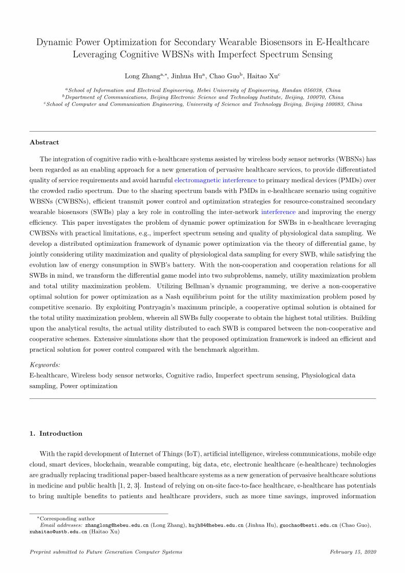
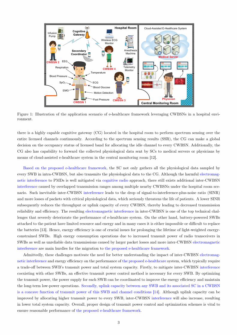
One of the most promising and enabling approaches to solve the aforementioned challenges is to integrate cognitiveradio into WBSN-assisted e-healthcare systems, to design an e-healthcare framework leveraging cognitive WBSNs(CWBSNs) [8, 9, 7, 10, 11]. In a traditional cognitive radio system, unlicensed secondary users are allowed toopportunistically access the idle band of spectrum temporarily unused by licensed or primary users without interferingwith them. For an emerging e-healthcare framework leveraging CWBSNs, patient-centric biosensors with low priorityacting as secondary users are permitted to sense, identify, and access the spectrum opportunities while incurring noharmful interference to the coexisting primary users, i.e., primary medical devices (PMDs) with higher priority. Theresulting e-healthcare based on the cognitive radio idea has been envisioned as a new solution for next generationhealthcare services, and also has the potential to improve the spectrum efficiency performance of system. Fig. 1illustrates a typical application scenario of our proposed e-healthcare system in a hospital environment including ahospital room and a central monitoring room. In the considered scenario, four underlay CWBSNs are coexisting witha primary system sharing the authorized spectrum simultaneously in the hospital room. The primary system consistsof four protected PMDs, i.e., wireless ECG monitor, infusion pump, anesthesia machine, and telemetry monitor,which are sensitive to the electromagnetic interference effect. In intra-CWBSN, several secondary wearable biosensors(SWBs) are attached on a patient to sense his or her physiological data, and further send the collected data to anear-body secondary coordinator (SC) through uplink transmission. To obtain the spectrum opportunities for SWBs,

1In what follows, unless otherwise stated, we use the terms “electromagnetic interference” and “interference” interchangeably.

2

BIOSENSORBIOSENSOR

BIOSENSORBIOSENSOR

BIOSENSORBIOSENSOR

Figure 1: Illustration of the application scenario of e-healthcare framework leveraging CWBSNs in a hospital envi-ronment.

there is a highly capable cognitive gateway (CG) located in the hospital room to perform spectrum sensing over theentire licensed channels continuously. According to the spectrum sensing results (SSR), the CG can make a globaldecision on the occupancy status of licensed band for allocating the idle channel to every CWBSN. Additionally, theCG also has capability to forward the collected physiological data sent by SCs to medical servers or physicians bymeans of cloud-assisted e-healthcare system in the central monitoring room [12].

Based on the proposed e-healthcare framework, the SC not only gathers all the physiological data sampled byevery SWB in intra-CWBSN, but also transmits the physiological data to the CG. Although the harmful electromag-netic interference to PMDs is well mitigated via cognitive radio approach, there still exists additional inter-CWBSNinterference caused by overlapped transmission ranges among multiple nearby CWBSNs under the hospital room sce-nario. Such inevitable inter-CWBSN interference leads to the drop of signal-to-interference-plus-noise ratio (SINR)and more losses of packets with critical physiological data, which seriously threatens the life of patients. A lower SINRsubsequently reduces the throughput or uplink capacity of every CWBSN, thereby leading to decreased transmissionreliability and efficiency. The resulting electromagnetic interference in inter-CWBSN is one of the top technical chal-lenges that severely deteriorate the performance of e-healthcare system. On the other hand, battery-powered SWBsattached to the patient have limited resource and energy and in many cases it is either impossible or difficult to replacethe batteries [13]. Hence, energy efficiency is one of crucial issues for prolonging the lifetime of light-weighted energy-constrained SWBs. High energy consumption operations due to increased transmit power of radio transceivers inSWBs as well as unreliable data transmissions caused by larger packet losses and more inter-CWBSN electromagneticinterference are main hurdles for the migration to the proposed e-healthcare framework.

Admittedly, these challenges motivate the need for better understanding the impact of inter-CWBSN electromag-netic interference and energy efficiency on the performance of the proposed e-healthcare system, which typically requirea trade-off between SWB’s transmit power and total system capacity. Firstly, to mitigate inter-CWBSN interferencecoexisting with other SWBs, an effective transmit power control method is necessary for every SWB. By optimizingthe transmit power, the power supply for each SWB can be coordinated to improve the energy efficiency and maintainthe long-term low-power operations. Secondly, uplink capacity between any SWB and its associated SC in a CWBSNis a concave function of transmit power of this SWB and channel conditions [14]. Although uplink capacity can beimproved by allocating higher transmit power to every SWB, inter-CWBSN interference will also increase, resultingin lower total system capacity. Overall, proper design of transmit power control and optimization schemes is vital toensure reasonable performance of the proposed e-healthcare framework.

3

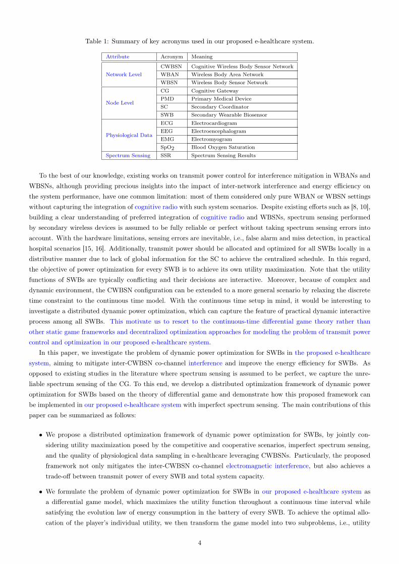
Table 1: Summary of key acronyms used in our proposed e-healthcare system.

Attribute Acronym Meaning

Network LevelCWBSN Cognitive Wireless Body Sensor NetworkWBAN Wireless Body Area NetworkWBSN Wireless Body Sensor Network

Node Level

CG Cognitive GatewayPMD Primary Medical DeviceSC Secondary CoordinatorSWB Secondary Wearable Biosensor

Physiological Data

ECG ElectrocardiogramEEG ElectroencephalogramEMG ElectromyogramSpO2 Blood Oxygen Saturation

Spectrum Sensing SSR Spectrum Sensing Results

To the best of our knowledge, existing works on transmit power control for interference mitigation in WBANs andWBSNs, although providing precious insights into the impact of inter-network interference and energy efficiency onthe system performance, have one common limitation: most of them considered only pure WBAN or WBSN settingswithout capturing the integration of cognitive radio with such system scenarios. Despite existing efforts such as [8, 10],building a clear understanding of preferred integration of cognitive radio and WBSNs, spectrum sensing performedby secondary wireless devices is assumed to be fully reliable or perfect without taking spectrum sensing errors intoaccount. With the hardware limitations, sensing errors are inevitable, i.e., false alarm and miss detection, in practicalhospital scenarios [15, 16]. Additionally, transmit power should be allocated and optimized for all SWBs locally in adistributive manner due to lack of global information for the SC to achieve the centralized schedule. In this regard,the objective of power optimization for every SWB is to achieve its own utility maximization. Note that the utilityfunctions of SWBs are typically conflicting and their decisions are interactive. Moreover, because of complex anddynamic environment, the CWBSN configuration can be extended to a more general scenario by relaxing the discretetime constraint to the continuous time model. With the continuous time setup in mind, it would be interesting toinvestigate a distributed dynamic power optimization, which can capture the feature of practical dynamic interactiveprocess among all SWBs. This motivate us to resort to the continuous-time differential game theory rather thanother static game frameworks and decentralized optimization approaches for modeling the problem of transmit powercontrol and optimization in our proposed e-healthcare system.

In this paper, we investigate the problem of dynamic power optimization for SWBs in the proposed e-healthcaresystem, aiming to mitigate inter-CWBSN co-channel interference and improve the energy efficiency for SWBs. Asopposed to existing studies in the literature where spectrum sensing is assumed to be perfect, we capture the unre-liable spectrum sensing of the CG. To this end, we develop a distributed optimization framework of dynamic poweroptimization for SWBs based on the theory of differential game and demonstrate how this proposed framework canbe implemented in our proposed e-healthcare system with imperfect spectrum sensing. The main contributions of thispaper can be summarized as follows:

• We propose a distributed optimization framework of dynamic power optimization for SWBs, by jointly con-sidering utility maximization posed by the competitive and cooperative scenarios, imperfect spectrum sensing,and the quality of physiological data sampling in e-healthcare leveraging CWBSNs. Particularly, the proposedframework not only mitigates the inter-CWBSN co-channel electromagnetic interference, but also achieves atrade-off between transmit power of every SWB and total system capacity.

• We formulate the problem of dynamic power optimization for SWBs in our proposed e-healthcare system asa differential game model, which maximizes the utility function throughout a continuous time interval whilesatisfying the evolution law of energy consumption in the battery of every SWB. To achieve the optimal allo-cation of the player’s individual utility, we then transform the game model into two subproblems, i.e., utility

4

maximization problem and total utility maximization problem, in terms of the competitive and fully cooperativescenarios for each SWB under the proposed game framework.

• For the utility maximization problem in the competitive scenario, the non-cooperative optimal solution forpower optimization is derived as a unique Nash equilibrium (NE) point via Bellman’s dynamic programming.Meanwhile, we further obtain the cooperative optimal solution for power optimization with respect to thetotal utility maximization problem in cooperative scenarios by invoking Pontryagin’s maximum principle. Wealso analyze the performance of dynamic power optimization according to the non-cooperation and cooperationrelations for SWBs. Our analysis provides quantitative insights on the impact of non-cooperation and cooperationrelations on the optimal power and the actual utility gained by each player.

The key acronyms and main notations used throughout this paper are summarized in Table 1 and Table 2 for theease of reference. The remainder of this paper is organized as follows. In Section 2, we provide an overview of therelated work. Section 3 presents the system model including system configuration, imperfect spectrum sensing model,and physiological data sampling model. In Section 4, we propose the dynamic power optimization framework, andderive the non-cooperative and cooperative optimal solutions. Moreover, we discuss and analyze the utilities of thenon-cooperative and cooperative dynamic power optimization. Simulation results are provided in Section 5, and weconclude the paper in Section 6.

2. Related Work

In the past few years, a number of studies have investigated the problem of transmit power control in WBANs andWBSNs for interference management from different perspectives, including link quality [17, 13, 18], energy harvesting[19], and relay selection [20, 21].

By analyzing the properties of link states via the received signal strength indicator (RSSI), Kim and Eom in [17]proposed a link-state-estimation-based power control scheme, which enables the transceiver of sensor node to adaptits transmit power level and target the RSSI threshold range. In [13], Zang et al. developed an accelerometer-aidedtransmit power control mechanism by incorporating the impact of human body movement on link quality measured bythe receiving RSSI value. The local accelerometer as a common WBAN device was utilized to acquire the periodic linkquality information without generating additional costs. With the aid of the hybrid strategy by jointly consideringclosed-loop control and posture/motion detection, Fernandes et al. in [18] devised a proactive power control method,which uses the RSSI value and the acceleration signal to predict the fading signal and to determine the position ofwearable devices during the gait cycle of human body, respectively.

Different from the link quality-aware power control approaches, Liu et al. in [19] proposed a two-phase resourceallocation scheme, to jointly optimize the allocation of transmit power, source rate, and time slots in the context ofenergy harvesting-powered WBANs. On the basis of the time-varying and heterogeneous energy harvesting states, thelong- and short-term QoS performances in two adopted phases were markedly improved by analyzing the statisticalknowledge of energy harvesting. In [20], Dong and Smith presented an integrated scheme of joint two-hop relayselection and power control by taking advantage of channel prediction, to strike a desired balance in the trade-offbetween power saving and interference mitigation. In [21], a relay-aided transmit power control method was designed,which can automatically switch the transmitter’s transmission strategy between direct transmission and relay-aidedtransmission according to the on-body channel conditions. All the above works in [13, 17, 18, 19, 20, 21], even thoughthey provide valuable insights on the potential of bringing power control into WBANs and WBSNs, do so withoutcapturing the integration of dynamic spectrum access with the considered system scenarios, to protect the primarydevices with high priority from harmful interference.

Alternatively, there have been some existing researches in the literature analyzing the performance of power controlin WBANs by using machine learning, to enable adaptive learning and intelligent decision making. To combat thejamming attacks, Chen et al. [22] developed a reinforcement learning-based power control scheme for in-body sensors.

5

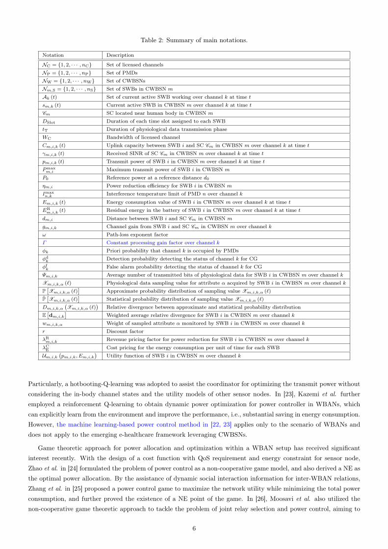
Table 2: Summary of main notations.

Notation Description

NC = {1, 2, · · · , nC} Set of licensed channelsNP = {1, 2, · · · , nP} Set of PMDsNW = {1, 2, · · · , nW} Set of CWBSNsNm,S = {1, 2, · · · , nS} Set of SWBs in CWBSN m

Ak (t) Set of current active SWB working over channel k at time tsm,k (t) Current active SWB in CWBSN m over channel k at time tCm SC located near human body in CWBSN m

DSlot Duration of each time slot assigned to each SWBtT Duration of physiological data transmission phaseWC Bandwidth of licensed channelCm,i,k (t) Uplink capacity between SWB i and SC Cm in CWBSN m over channel k at time tγm,i,k (t) Received SINR of SC Cm in CWBSN m over channel k at time tpm,i,k (t) Transmit power of SWB i in CWBSN m over channel k at time tPmaxm,i Maximum transmit power of SWB i in CWBSN m

P0 Reference power at a reference distance d0ηm,i Power reduction efficiency for SWB i in CWBSN m

Imaxn,k Interference temperature limit of PMD n over channel k

Em,i,k (t) Energy consumption value of SWB i in CWBSN m over channel k at time tERm,i,k (t) Residual energy in the battery of SWB i in CWBSN m over channel k at time t

dm,i Distance between SWB i and SC Cm in CWBSN m

gm,i,k Channel gain from SWB i and SC Cm in CWBSN m over channel kω Path-loss exponent factorΓ Constant processing gain factor over channel kφk Priori probability that channel k is occupied by PMDsφdk Detection probability detecting the status of channel k for CGφfk False alarm probability detecting the status of channel k for CGΨm,i,k Average number of transmitted bits of physiological data for SWB i in CWBSN m over channel kXm,i,k,α (`) Physiological data sampling value for attribute α acquired by SWB i in CWBSN m over channel kP[Xm,i,k,α (`)

]Approximate probability distribution of sampling value Xm,i,k,α (`)

P[Xm,i,k,α (`)

]Statistical probability distribution of sampling value Xm,i,k,α (`)

Dm,i,k,α(Xm,i,k,α (`)

)Relative divergence between approximate and statistical probability distribution

E[dm,i,k

]Weighted average relative divergence for SWB i in CWBSN m over channel k

wm,i,k,α Weight of sampled attribute α monitored by SWB i in CWBSN m over channel kr Discount factorλRm,i,k Revenue pricing factor for power reduction for SWB i in CWBSN m over channel k

λCE Cost pricing for the energy consumption per unit of time for each SWBUm,i,k

(pm,i,k, Em,i,k

)Utility function of SWB i in CWBSN m over channel k

Particularly, a hotbooting-Q-learning was adopted to assist the coordinator for optimizing the transmit power withoutconsidering the in-body channel states and the utility models of other sensor nodes. In [23], Kazemi et al. furtheremployed a reinforcement Q-learning to obtain dynamic power optimization for power controller in WBANs, whichcan explicitly learn from the environment and improve the performance, i.e., substantial saving in energy consumption.However, the machine learning-based power control method in [22, 23] applies only to the scenario of WBANs anddoes not apply to the emerging e-healthcare framework leveraging CWBSNs.

Game theoretic approach for power allocation and optimization within a WBAN setup has received significantinterest recently. With the design of a cost function with QoS requirement and energy constraint for sensor node,Zhao et al. in [24] formulated the problem of power control as a non-cooperative game model, and also derived a NE asthe optimal power allocation. By the assistance of dynamic social interaction information for inter-WBAN relations,Zhang et al. in [25] proposed a power control game to maximize the network utility while minimizing the total powerconsumption, and further proved the existence of a NE point of the game. In [26], Moosavi et al. also utilized thenon-cooperative game theoretic approach to tackle the problem of joint relay selection and power control, aiming to

6

obtain the maximized energy efficiency and meet the QoS requirements. Similarly, the idea of using non-cooperativegame framework as an analytical method to optimize the transmit power in WBANs has been further explored in[27, 28]. However, the game theoretic models presented in the these works [24, 25, 26, 27, 28] were just focused onthe non-cooperative scenarios, without capturing the potential benefits of designing cooperative power optimizationstrategies. Moreover, the existing game theoretic methods using the static game framework cannot exactly capturehow to dynamically optimize the transmit power with respect to the current instant time in a more realistic anddynamic environment. By contrast, we extensively consider the actual behaviors of individual game players in termsof the competitive and cooperative scenarios, and investigate their impacts on the performance of dynamic poweroptimization.

To date, only rare few efforts have been devoted to address the issue of power allocation and optimization ine-healthcare systems by tightly integrating cognitive radio with WBSNs, to protect PMDs from harmful interfer-ence. Considering the issues of harmful interference to primary medical devices and differentiated QoS requirements,Phunchongharn et al. in [8] demonstrated the potential advantages of using cognitive radio in the design of wire-less communication systems, particularly for e-healthcare applications in a hospital environment. With this idea,to obtain the effective channel access, an interference-aware time slotted handshaking protocol was designed for theprimary and secondary medical devices with desired QoS differentiation. The proposed protocol only extended thetraditional carrier sense multiple access with collision avoidance mechanism to the cognitive radio based e-healthcarescenario. This paper is quite attractive and instructive, although it does not investigate the power optimization issuethat reveals an interplay between transmit power of low priority medical devices and total system capacity. In [10],Naeem et al. focused on a modern automated hospital scenario with various wireless devices, e.g., wireless sensordevices, personal wireless hubs, central controllers, etc, in healthcare facilities. By applying the cognitive radio idea,a limited set of unlicensed secondary wireless devices (i.e., wireless sensor devices and personal wireless hubs) wasallowed to exploit the unused spectrum that was assigned to the licensed primary wireless devices, including all otherhealthcare equipments. Depending on these settings, the authors presented a framework of interference-aware jointpower control and assignment of multiple personal wireless hubs, which can maximize the total transmission datarate under the acceptable interference constraints. Despite its novel insights, the joint optimization framework in[10] is formulated bearing in mind an ideal assumption of perfect spectrum sensing carried out by secondary wirelessdevices. Nevertheless, perfect spectrum sensing with none of spectrum sensing errors is extremely difficult to achievein practical CWBSN-based e-healthcare systems. To that end, the work presented in this paper adopts more practicallimitations, e.g., imperfect spectrum sensing and the quality of physiological data sampling, to investigate the issueof transmit power control and optimization in the proposed e-healthcare system.

To sum up, although a lot of works have been carried out on the power control problem in pure WBAN/WBSNscenarios extensively as well as only limited efforts have focused on the attempts at a coupling of cognitive radio ande-healthcare, there still seems to be a gap between e-healthcare systems and efficient integration of cognitive radiowith WBSNs. To be more concrete, there exist several fundamental technical difficulties to deal with:

• Most of the existing studies involve the static game framework without capturing the practical constraints ofdynamic interactive actions among all the sensor nodes subject to the dynamic time-varying transmit poweradjustment in WBANs. From practical view points, the update of transmit power level for each sensor nodeshould be continuous in time. Hence, it is imperative to develop a general optimization framework to achievedynamic power control via the continuous-time differential game theory.

• In practice, sensing errors for spectrum sensing conducted by secondary wireless devices in e-healthcare systemsthat considering the integration of cognitive radio and WBSNs are actually unavoidable as a result of thelimitation on hardware. However, it is a widespread assumption in the existing works that spectrum sensingis fully reliable or perfect without any explicit errors. Hence, it is necessary to reconsider spectrum sensing toadapt to the practical environment.

7

T

T

t t

nj

t t Dt

Figure 2: The time-slotted frame structure.

In this paper, we tackle the above issues by providing a distributed optimization framework of dynamic powercontrol for SWBs in our proposed e-healthcare system with imperfect spectrum sensing.

3. System Model

3.1. System Configuration

Consider an application scenario of e-healthcare framework leveraging CWBSNs in a hospital environment witha central monitoring room and a hospital room as shown in Fig. 1. We concentrate on one CG and nW underlayCWBSNs, denoted by NW = {1, 2, · · · , nW}, coexisting with a primary system in a hospital room sharing the autho-rized spectrum in the same frequency band simultaneously. The whole authorized spectrum band is divided into nClicensed channels with equal bandwidth WC, denoted by NC = {1, 2, · · · , nC}. We assume that the CG is equippedwith an omnidirectional antenna, a predefined common control channel, and an energy detector that continuouslysenses the entire licensed channels through local real-time measurements. Based on the SSR, the CG makes decisionto determine whether or not the licensed channels are vacant, for allocating the unoccupied channel to each CWBSNvia the common control channel. The primary system consists of nP PMDs, denoted by NP = {1, 2, · · · , nP}, whichhave the full privilege of accessing the licensed channels from time to time. Particularly, the occupation time lengthof every licensed channel assigned to a PMD follows an independent and identically distributed (i.i.d.) alternatingON-OFF process. The OFF state indicates the idle state where unoccupied channel can be freely accessed by eachCWBSN.

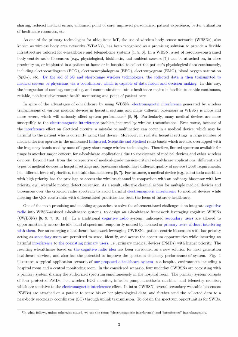
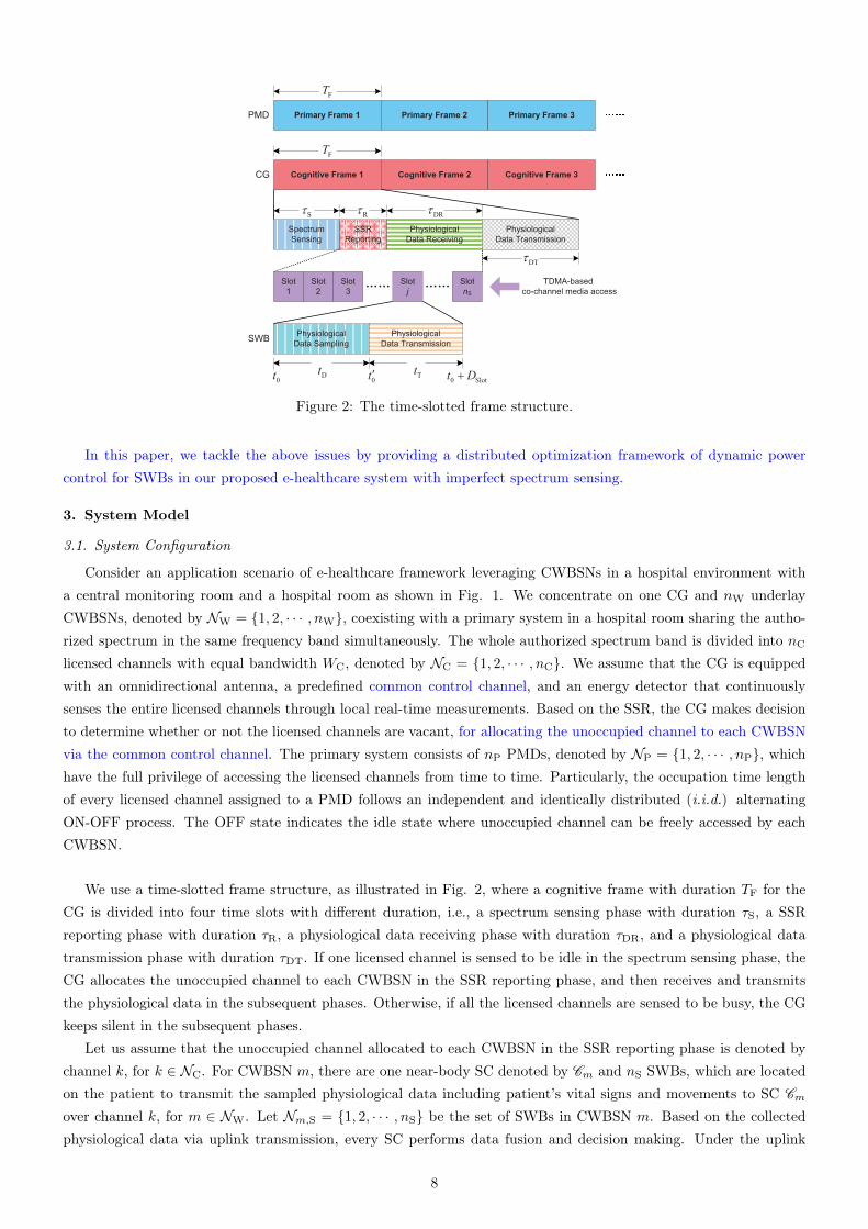
We use a time-slotted frame structure, as illustrated in Fig. 2, where a cognitive frame with duration TF for theCG is divided into four time slots with different duration, i.e., a spectrum sensing phase with duration τS, a SSRreporting phase with duration τR, a physiological data receiving phase with duration τDR, and a physiological datatransmission phase with duration τDT. If one licensed channel is sensed to be idle in the spectrum sensing phase, theCG allocates the unoccupied channel to each CWBSN in the SSR reporting phase, and then receives and transmitsthe physiological data in the subsequent phases. Otherwise, if all the licensed channels are sensed to be busy, the CGkeeps silent in the subsequent phases.

Let us assume that the unoccupied channel allocated to each CWBSN in the SSR reporting phase is denoted bychannel k, for k ∈ NC. For CWBSN m, there are one near-body SC denoted by Cm and nS SWBs, which are locatedon the patient to transmit the sampled physiological data including patient’s vital signs and movements to SC Cm

over channel k, for m ∈ NW. Let Nm,S = {1, 2, · · · , nS} be the set of SWBs in CWBSN m. Based on the collectedphysiological data via uplink transmission, every SC performs data fusion and decision making. Under the uplink

8

nj

j n

j n

j n

j n

(a) Ordered channel access

nj

j n

j n

j n

n j

(b) Disordered channel access

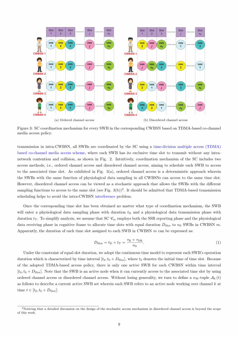
Figure 3: SC coordination mechanism for every SWB in the corresponding CWBSN based on TDMA-based co-channelmedia access policy.

transmission in intra-CWBSN, all SWBs are coordinated by the SC using a time-division multiple access (TDMA)based co-channel media access scheme, where each SWB has its exclusive time slot to transmit without any intra-network contention and collision, as shown in Fig. 2. Intuitively, coordination mechanism of the SC includes twoaccess methods, i.e., ordered channel access and disordered channel access, aiming to schedule each SWB to accessto the associated time slot. As exhibited in Fig. 3(a), ordered channel access is a deterministic approach whereinthe SWBs with the same function of physiological data sampling in all CWBSNs can access to the same time slot.However, disordered channel access can be viewed as a stochastic approach that allows the SWBs with the differentsampling functions to access to the same slot (see Fig. 3(b))2. It should be admitted that TDMA-based transmissionscheduling helps to avoid the intra-CWBSN interference problem.

Once the corresponding time slot has been obtained no matter what type of coordination mechanism, the SWBwill enter a physiological data sampling phase with duration tD and a physiological data transmission phase withduration tT. To simplify analysis, we assume that SC Cm employs both the SSR reporting phase and the physiologicaldata receiving phase in cognitive frame to allocate time slots with equal duration DSlot to nS SWBs in CWBSN m.Apparently, the duration of each time slot assigned to each SWB in CWBSN m can be expressed as:

DSlot = tD + tT =τR + τDR

nS. (1)

Under the constraint of equal slot duration, we adopt the continuous time model to represent each SWB’s operationduration which is characterized by time interval [t0, t0 +DSlot], where t0 denotes the initial time of time slot. Becauseof the adopted TDMA-based access policy, there is only one active SWB for each CWBSN within time interval[t0, t0 +DSlot]. Note that the SWB is an active node when it can currently access to the associated time slot by usingordered channel access or disordered channel access. Without losing generality, we turn to define a nW-tuple Ak (t)as follows to describe a current active SWB set wherein each SWB refers to an active node working over channel k attime t ∈ [t0, t0 +DSlot]:

2Noticing that a detailed discussion on the design of the stochastic access mechanism in disordered channel access is beyond the scopeof this work.

9

Ak (t) = {s1,k (t) , s2,k (t) , · · · , sm,k (t) , · · · , snW,k (t)} , ∀m ∈ NW,∀k ∈ NC, (2)

where sm,k (t) is the current active SWB in CWBSN m over channel k at time t. For the notational brevity, wedenote the current active SWB in CWBSN m over channel k at time t by SWB i, i.e., i , sm,k (t), for i ∈ Nm,S andsm,k (t) ∈ Ak (t). We further use t′0 to stand for an initial time of the physiological data transmission phase for everySWB as shown in Fig. 2. Thus, the duration of the physiological data transmission phase can be specified by timeinterval [t′0, t0 +DSlot]. Apparently, we can easily have tT = DSlot + t0 − t′0. To deal with co-channel electromagneticinterference problem in inter-CWBSN, we turn our attention to the uplink transmission by exploring transmit poweroptimization mechanism for the current active SWB during the physiological data transmission phase. In fact, thetransmit power pm,i,k (t) of SWB i in CWBSN m over channel k at time t ∈ [t′0, t0 +DSlot] is adjusted in a continuousway but is also limited by a maximum value Pmax

m,i . Based on the Friis formula in free space, similar to [29, 30], themaximum transmit power of SWB i in CWBSN m can be approximately given by:

Pmaxm,i (dBm) = P0 (dBm)− 10ω log10

(dm,id0

), (3)

where P0 (in dBm) is the receiving reference power by SC Cm at a reference distance d0, dm,i is the distance betweenSWB i and SC Cm in CWBSN m, and ω ≥ 2 is the path-loss exponent. We assume that the uplink wireless channelstate is expected to be unchanged during time interval [t′0, t0 +DSlot], and is subject to the distance dependent powerattenuation. Thereby, we can use a slow flat fading channel model to characterize the channel gain from SWB i toSC Cm in CWBSN m over channel k, which is given as gm,i,k = d−ωm,i. In terms of the current active SWB set, thereceived SINR of SC Cm in CWBSN m over channel k at time t ∈ [t′0, t0 +DSlot] is formulated as:

γm,i,k (t) =pm,i,k (t) gm,i,k

nW∑j=1,j 6=m

pj,sj(t),k (t) gj,sj(t),k + n0

, (4)

where pj,sj(t),k (t) is the instant transmit power of SWB sj,k (t) in CWBSN j over channel k at time t, gj,sj(t),k is theinterference gain from SWB sj,k (t) in CWBSN j to SC Cm over channel k, and n0 is the background noise powerspectral density at SC Cm. According to Shannon’s capacity formula, the uplink capacity (in bps) between SWB i

and SC Cm in CWBSN m over channel k at time t can be calculated by:

Cm,i,k (t) =WC log2 (1 + Γγm,i,k (t)) , (5)

where Γ = −β1/ log2 (β2 · BER) is the constant processing gain factor with constants β1 and β2 depending on accept-able bit error rate (BER), modulation strategy, and coding scheme over channel k. Although the overall spectrum-utilization efficiency has been improved, the uplink transmission for each SWB in an opportunistic way during thephysiological data transmission phase may also generate the extra interference to PMDs. In this case, the interferencepower constraint should be imposed to protect PMDs from unavoidable electromagnetic interference caused by allSWBs. For PMD n, the accumulated interference caused by the current active SWB set working over channel k attime t must be kept below the interference temperature limit Imax

n,k given as follows [31]:

nW∑m=1

pm,sm,k(t),k (t) gn,sm,k(t),k ≤ Imaxn,k , ∀n ∈ NP,∀m ∈ NW, (6)

where pm,sm,k(t),k (t) is the transmit power of SWB i in CWBSN m over channel k at time t, and gn,sm,k(t),k is thechannel gain from SWB i in CWBSN m to PMD n over channel k.

10

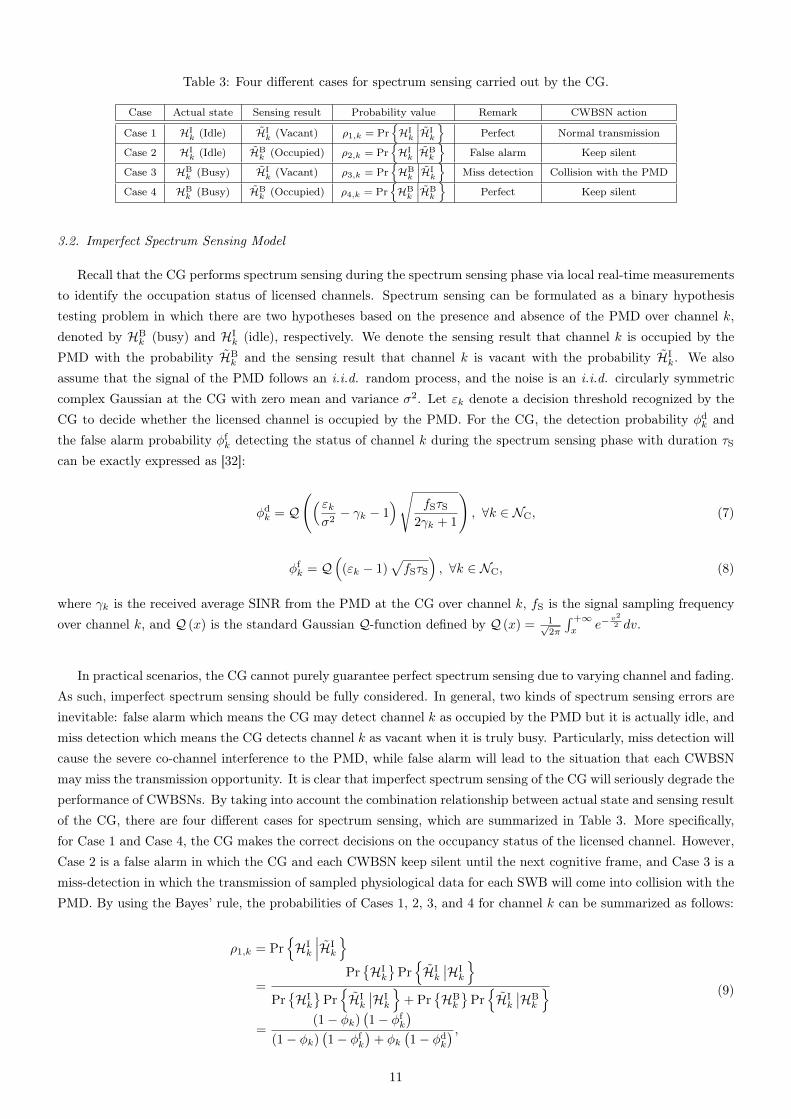
Table 3: Four different cases for spectrum sensing carried out by the CG.

Case Actual state Sensing result Probability value Remark CWBSN action

Case 1 HIk (Idle) HI

k (Vacant) ρ1,k = Pr{HIk

∣∣∣HIk

}Perfect Normal transmission

Case 2 HIk (Idle) HB

k (Occupied) ρ2,k = Pr{HIk

∣∣∣HBk

}False alarm Keep silent

Case 3 HBk (Busy) HI

k (Vacant) ρ3,k = Pr{HBk

∣∣∣HIk

}Miss detection Collision with the PMD

Case 4 HBk (Busy) HB

k (Occupied) ρ4,k = Pr{HBk

∣∣∣HBk

}Perfect Keep silent

3.2. Imperfect Spectrum Sensing Model

Recall that the CG performs spectrum sensing during the spectrum sensing phase via local real-time measurementsto identify the occupation status of licensed channels. Spectrum sensing can be formulated as a binary hypothesistesting problem in which there are two hypotheses based on the presence and absence of the PMD over channel k,denoted by HB

k (busy) and HIk (idle), respectively. We denote the sensing result that channel k is occupied by the

PMD with the probability HBk and the sensing result that channel k is vacant with the probability HI

k. We alsoassume that the signal of the PMD follows an i.i.d. random process, and the noise is an i.i.d. circularly symmetriccomplex Gaussian at the CG with zero mean and variance σ2. Let εk denote a decision threshold recognized by theCG to decide whether the licensed channel is occupied by the PMD. For the CG, the detection probability φdk andthe false alarm probability φfk detecting the status of channel k during the spectrum sensing phase with duration τScan be exactly expressed as [32]:

φdk = Q

(( εkσ2− γk − 1

)√ fSτS2γk + 1

), ∀k ∈ NC, (7)

φfk = Q((εk − 1)

√fSτS

), ∀k ∈ NC, (8)

where γk is the received average SINR from the PMD at the CG over channel k, fS is the signal sampling frequencyover channel k, and Q (x) is the standard Gaussian Q-function defined by Q (x) = 1√

2π

∫ +∞x

e−v2

2 dv.

In practical scenarios, the CG cannot purely guarantee perfect spectrum sensing due to varying channel and fading.As such, imperfect spectrum sensing should be fully considered. In general, two kinds of spectrum sensing errors areinevitable: false alarm which means the CG may detect channel k as occupied by the PMD but it is actually idle, andmiss detection which means the CG detects channel k as vacant when it is truly busy. Particularly, miss detection willcause the severe co-channel interference to the PMD, while false alarm will lead to the situation that each CWBSNmay miss the transmission opportunity. It is clear that imperfect spectrum sensing of the CG will seriously degrade theperformance of CWBSNs. By taking into account the combination relationship between actual state and sensing resultof the CG, there are four different cases for spectrum sensing, which are summarized in Table 3. More specifically,for Case 1 and Case 4, the CG makes the correct decisions on the occupancy status of the licensed channel. However,Case 2 is a false alarm in which the CG and each CWBSN keep silent until the next cognitive frame, and Case 3 is amiss-detection in which the transmission of sampled physiological data for each SWB will come into collision with thePMD. By using the Bayes’ rule, the probabilities of Cases 1, 2, 3, and 4 for channel k can be summarized as follows:

ρ1,k = Pr{HIk

∣∣∣HIk

}=

Pr{HIk

}Pr{HIk

∣∣HIk

}Pr{HIk

}Pr{HIk

∣∣HIk

}+ Pr

{HBk

}Pr{HIk

∣∣HBk

}=

(1− φk)(1− φfk

)(1− φk)

(1− φfk

)+ φk

(1− φdk

) ,(9)

11

ρ2,k = Pr{HIk

∣∣∣HBk

}=

Pr{HIk

}Pr{HBk

∣∣HIk

}Pr{HIk

}Pr{HBk

∣∣HIk

}+ Pr

{HBk

}Pr{HBk

∣∣HBk

}=

(1− φk)φfk(1− φk)φfk + φkφdk

,

(10)

ρ3,k = Pr{HBk

∣∣∣HIk

}=

Pr{HBk

}Pr{HIk

∣∣HBk

}Pr{HBk

}Pr{HIk

∣∣HBk

}+ Pr

{HIk

}Pr{HIk

∣∣HIk

}=

φk(1− φdk

)φk(1− φdk

)+ (1− φk)

(1− φfk

) ,(11)

ρ4,k = Pr{HBk

∣∣∣HBk

}=

Pr{HBk

}Pr{HBk

∣∣HBk

}Pr{HBk

}Pr{HBk

∣∣HBk

}+ Pr

{HIk

}Pr{HBk

∣∣HIk

}=

φkφdk

φkφdk + (1− φk)φfk,

(12)

where φk is the priori probability that channel k is occupied by the PMD. Based on the probabilities of Cases 1, 2, 3,and 4 and the CWBSN actions as listed in Table 3, we notice that there is only Case 1 achieving normal transmissionduring the SSR reporting phase and the physiological data receiving phase. Here, we focus on the uplink transmissionof collected physiological data in each CWBSN. Let Ψm,i,k, Ψm,k, and Ψk represent the average number of transmittedbits of physiological data for SWB i in CWBSN m, for CWBSN m, and for nW CWBSNs over channel k, respectively.For SWB i in CWBSN m over channel k, the average number of transmitted bits of physiological data within equalslot duration DSlot assigned to each SWB can be approximately calculated as follows [33]:

Ψm,i,k = DSlotWC log2 (1 + Γγm,i,k (t)) Pr{HIk

∣∣∣HIk

}. (13)

Likewise, the average number of transmitted bits of physiological data for CWBSN m and nW CWBSNs over channelk, can be derived as Ψm,k =

nS∑i=1

Ψm,i,k and Ψk =nW∑m=1

nS∑i=1

Ψm,i,k, respectively.

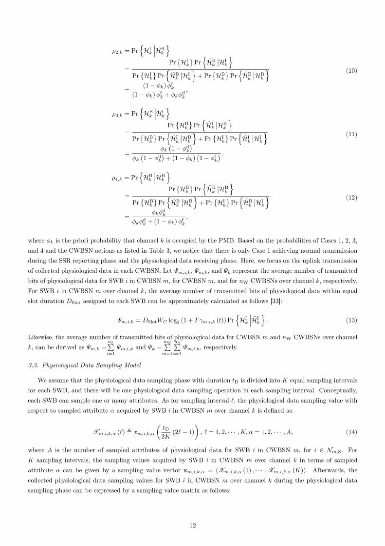
3.3. Physiological Data Sampling Model

We assume that the physiological data sampling phase with duration tD is divided into K equal sampling intervalsfor each SWB, and there will be one physiological data sampling operation in each sampling interval. Conceptually,each SWB can sample one or many attributes. As for sampling interval `, the physiological data sampling value withrespect to sampled attribute α acquired by SWB i in CWBSN m over channel k is defined as:

Xm,i,k,α (`) , xm,i,k,α

(tD2K

(2`− 1)

), ` = 1, 2, · · · ,K, α = 1, 2, · · · , A, (14)

where A is the number of sampled attributes of physiological data for SWB i in CWBSN m, for i ∈ Nm,S. ForK sampling intervals, the sampling values acquired by SWB i in CWBSN m over channel k in terms of sampledattribute α can be given by a sampling value vector xm,i,k,α = (Xm,i,k,α (1) , · · · ,Xm,i,k,α (K)). Afterwards, thecollected physiological data sampling values for SWB i in CWBSN m over channel k during the physiological datasampling phase can be expressed by a sampling value matrix as follows:

12

Algorithm 1 Approximate Probability Distribution Generation AlgorithmInput: Sampling value vector xm,i,k,α = (Xm,i,k,α (1) , · · · ,Xm,i,k,α (K)).Output: Approximate probability distribution P [Xm,i,k,α (`)] = {ym,i,k,α (1) , · · · , ym,i,k,α (l) , · · · , ym,i,k,α (Lm,i,k,α)}.1: Sort sampling values within xm,i,k,α in an ascending order:

i) Set ℘m,i,k,α (1) = min {Xm,i,k,α (1) , · · · ,Xm,i,k,α (K)}.ii) Set ℘m,i,k,α (K) = max {Xm,i,k,α (1) , · · · ,Xm,i,k,α (K)}.iii) Obtain a sorted sequence ℘m,i,k,α (1) , ℘m,i,k,α (2) , ℘m,i,k,α (3) , · · · , ℘m,i,k,α (K).

2: Set auxiliary constant βminm,i,k,α > 0, for βmin

m,i,k,α < ℘m,i,k,α (1).3: Set auxiliary constant βmax

m,i,k,α > 0, for βmaxm,i,k,α > ℘m,i,k,α (K).

4: Divide interval[βminm,i,k,α, β

maxm,i,k,α

]into Lm,i,k,α equal subintervals:

βminm,i,k,α = Λ0 < Λ1 < Λ2 < · · · < ΛLm,i,k,α−1 < ΛLm,i,k,α = βmax

m,i,k,α.5: for l = 1 to Lm,i,k,α do

6: Λl − Λl−1 =βmaxm,i,k,α−βmin

m,i,k,α

Lm,i,k,α.

7: Calculate the number of sampling values within subinterval (Λl−1,Λl] denoted by zm,i,k,α (l).8: Calculate the probability of sampling value by ym,i,k,α (l) =

zm,i,k,α(l)

K.

9: end for10: return {ym,i,k,α (1) , · · · , ym,i,k,α (l) , · · · , ym,i,k,α (Lm,i,k,α)}.

Xm,i,k =

(xm,i,k,1 xm,i,k,2 · · · xm,i,k,α · · · xm,i,k,A

)T

=

xm,i,k,1(tD2K

)· · · xm,i,k,1

(tD2K (2`− 1)

)· · · xm,i,k,1

(tD2K (2K − 1)

)xm,i,k,2

(tD2K

)· · · xm,i,k,2

(tD2K (2`− 1)

)· · · xm,i,k,2

(tD2K (2K − 1)

)· · · · · · · · · · · · · · ·

xm,i,k,α(tD2K

)· · · xm,i,k,α

(tD2K (2`− 1)

)· · · xm,i,k,α

(tD2K (2K − 1)

)· · · · · · · · · · · · · · ·

xm,i,k,A(tD2K

)· · · xm,i,k,A

(tD2K (2`− 1)

)· · · xm,i,k,A

(tD2K (2K − 1)

)

A×K

.(15)

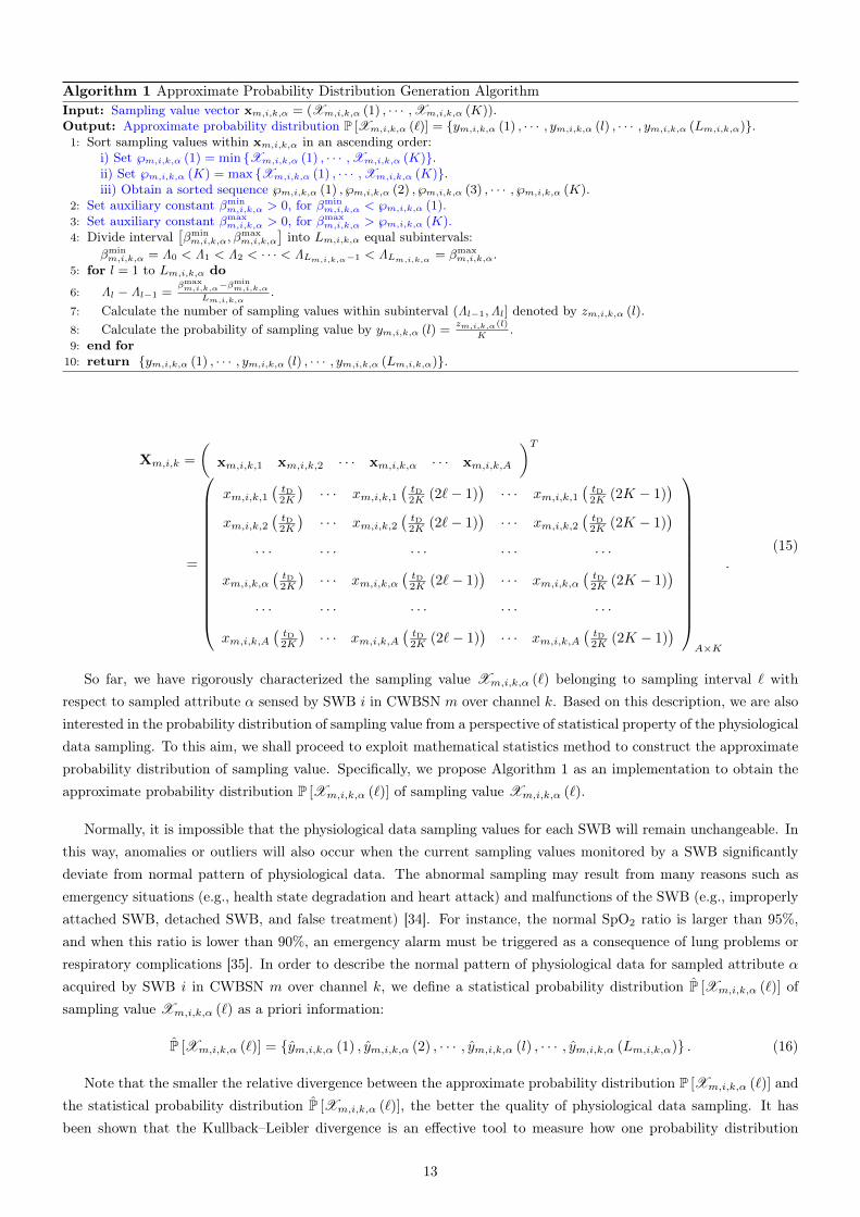
So far, we have rigorously characterized the sampling value Xm,i,k,α (`) belonging to sampling interval ` withrespect to sampled attribute α sensed by SWB i in CWBSN m over channel k. Based on this description, we are alsointerested in the probability distribution of sampling value from a perspective of statistical property of the physiologicaldata sampling. To this aim, we shall proceed to exploit mathematical statistics method to construct the approximateprobability distribution of sampling value. Specifically, we propose Algorithm 1 as an implementation to obtain theapproximate probability distribution P [Xm,i,k,α (`)] of sampling value Xm,i,k,α (`).

Normally, it is impossible that the physiological data sampling values for each SWB will remain unchangeable. Inthis way, anomalies or outliers will also occur when the current sampling values monitored by a SWB significantlydeviate from normal pattern of physiological data. The abnormal sampling may result from many reasons such asemergency situations (e.g., health state degradation and heart attack) and malfunctions of the SWB (e.g., improperlyattached SWB, detached SWB, and false treatment) [34]. For instance, the normal SpO2 ratio is larger than 95%,and when this ratio is lower than 90%, an emergency alarm must be triggered as a consequence of lung problems orrespiratory complications [35]. In order to describe the normal pattern of physiological data for sampled attribute αacquired by SWB i in CWBSN m over channel k, we define a statistical probability distribution P [Xm,i,k,α (`)] ofsampling value Xm,i,k,α (`) as a priori information:

P [Xm,i,k,α (`)] = {ym,i,k,α (1) , ym,i,k,α (2) , · · · , ym,i,k,α (l) , · · · , ym,i,k,α (Lm,i,k,α)} . (16)

Note that the smaller the relative divergence between the approximate probability distribution P [Xm,i,k,α (`)] andthe statistical probability distribution P [Xm,i,k,α (`)], the better the quality of physiological data sampling. It hasbeen shown that the Kullback–Leibler divergence is an effective tool to measure how one probability distribution

13

diverges from another reference probability distribution [36]. Thereby, the relative divergence between P [Xm,i,k,α (`)]

and P [Xm,i,k,α (`)] can be calculated under the Kullback–Leibler divergence framework as follows:

Dm,i,k,α (Xm,i,k,α (`)) ,Lm,i,k,α∑l=1

ym,i,k,α (l) log2ym,i,k,α (l)

ym,i,k,α (l). (17)

For A sampled attributes for SWB i in CWBSN m over channel k, the vector of the relative divergence is writtenby dm,i,k = (Dm,i,k,1 (Xm,i,k,1 (`)) , · · · , Dm,i,k,A (Xm,i,k,A (`))). Correspondingly, as for A sampled attributes, theweighted average relative divergence for SWB i in CWBSN m over channel k can be given by:

E [dm,i,k] =

A∑α=1

wm,i,k,αDm,i,k,α (Xm,i,k,α (`))

A∑α=1

wm,i,k,α

, (18)

where wm,i,k,α is the weight of sampled attribute α monitored by SWB i. Note that the weight of sampled attributeα reveals the importance of this attribute within all the sampled attributes. From (18), it is found that the smallerthe weighted average relative divergence, the better the quality of physiological data sampling. In this way, we wishto remark that the weighted average relative divergence can be used to characterize the quality of physiological datasampling for each SWB.

4. Dynamic Power Optimization Framework: Problem Formulation, Optimal Solution, and UtilityDiscussion

4.1. Problem Formulation

Owing to lack of global information for the SC to achieve the centralized schedule, transmit power should be allo-cated distributively by the current active SWBs. In general, the current active SWB has to reduce its transmit powerin order to cope with the inter-CWBSN co-channel electromagnetic interference problem. However, the reduction ofits own transmit power of the SWB would be attained at the expense of its own uplink capacity. This is due to the factthat the uplink capacity between the SWB and the SC is a concave function of current transmit power and channelconditions according to (5). Meanwhile, the objective of transmit power allocation for each SWB is to maximize itsown utility function. However, the utility functions of the current active SWBs are conflicting and their decisions areinteractive. Moreover, it will be more realistic to dynamically optimize the transmit power with respect to the currentinstant time. This motivates us to formulate the problem of dynamic power optimization for the current active SWBin each CWBSN as a differential game model.

Definition 1. (Differential Game Framework) The differential game theoretic framework for dynamic power opti-mization of the current active SWB set working over channel k at time t ∈ [t′0, t0 +DSlot] is defined as a 4-tuple:

Gk = {Ak (t) , {Pm,i,k (t)} , {Em,i,k (t)} , {Um,i,k (pm,i,k (t) , Em,i,k (t))}}i∈Ak(t) , ∀m ∈ NW,∀k ∈ NC, (19)

where,

• Player set Ak (t): Ak (t) = {s1,k (t) , s2,k (t) , · · · , snW,k (t)} is the set of the current active SWBs playing thegame. The players belong to the rational policy makers and act throughout a time interval in game Gk.

• Set of strategies {Pm,i,k (t)}: The strategy of a player is defined as its instant transmit power bounded by themaximum transmit power. Pm,i,k (t) = {pm,i,k (t) |∀t} is the strategy space of SWB i in CWBSN m over channelk.

• Set of states {Em,i,k (t)}: The state of a player refers to its instant energy consumption. Em,i,k (t) = {Em,i,k (t) |∀t}is the state space of SWB i, where Em,i,k (t) denotes the energy consumption value of SWB i in CWBSN m

over channel k.

14

• Set of utility functions {Um,i,k}: Um,i,k (pm,i,k, Em,i,k) is the utility function of SWB i in CWBSNm over channelk. The objective of each SWB is to maximize its utility function by rationally selecting optimal strategy andstate.

Note that differential game is a kind of continuous-time dynamic game wherein the utility function of the playerrelies on the strategy and the state of itself. Hereinafter, the terms “player” and “SWB” are all interchangeable, unlessexplicitly stated otherwise. Under this game framework, we put more emphasis on how to formulate the state spaceEm,i,k (t) and the utility function Um,i,k of SWB i in CWBSN m over channel k, respectively. To model the fact thatthe state space of SWB i needs to be defined to satisfy the state dynamics as in [37], we introduce a linear differentialequation to represent the state space of SWB i. Let ER

m,i,k (t) denote the residual energy in the battery of SWB i inCWBSN m over channel k at time t ∈ [t′0, t0 +DSlot]. Similar to [38], the evolution law of energy consumption in thebattery of SWB i can be defined by a linear differential equation as follows:

dEm,i,k (t)

dt= ER

m,i,k (t)− tTpm,i,k (t)− Em,i,k (t) . (20)

We next discuss how to characterize the utility function Um,i,k of SWB i in CWBSN m over channel k. With theconstraint of maximum value Pmax

m,i , the value of power reduction for SWB i is given by Pmaxm,i − pm,i,k (t). Hence, the

power reduction efficiency for SWB i at time t can be further expressed as:

ηm,i =Pmaxm,i − pm,i,k (t)

Pmaxm,i

. (21)

Let us revisit the weighted average relative divergence as mentioned in (18) that has been suggested to characterizethe quality of physiological data sampling for each SWB. Therefore, to formulate the revenue of power reduction foreach SWB, we attempt to devise a revenue pricing factor for power reduction performed by each SWB through a jointconsideration of both the power reduction efficiency and the weighted average relative divergence. This motivatesthe need for better understanding of the interplay between the power reduction efficiency and the weighted averagerelative divergence, which typically require a trade-off between them. From the point of view of trade-off strategy, asimilar design for pricing factor can be found in the formulation of energy-per-capacity factor [31]. Inspired by thiskind of trade-off design, the revenue pricing factor for every SWB in consideration should be highlighted as two pointsto achieve a reasonable result. On the one hand, it goes without saying that the more power reduction efficiency, thehigher pricing for a SWB, which means that a higher reward must be attached to that SWB due to its contribution topower reduction. On the other hand, the worse quality of physiological data sampling because of abnormal samplingincurred by emergency situations, the larger weighted average relative divergence for a SWB. Thus, the higher pricingcorresponding to a more reward should be offered for that SWB due to the importance of that SWB to reflect thecurrent emergency alarm, e.g., heart attack or health state degradation.

By combining these considerations, as for SWB i in CWBSNm over channel k, the revenue pricing factor for powerreduction is defined as the product of the power reduction efficiency and the weighted average relative divergence,which can be thus written as follows:

λRm,i,k , ηm,iE [dm,i,k] . (22)

Obviously, the increase of any values belonging to ηm,i or E [dm,i,k] will result in the more revenue pricing for SWBi. Consequently, the revenue of power reduction for SWB i in CWBSN m over channel k at time t ∈ [t′0, t0 +DSlot]

by attaining the product of the revenue pricing factor along with the value of power reduction for SWB i, i.e.:

ΘRm,i,k (t) = λRm,i,k

(Pmaxm,i − pm,i,k (t)

). (23)

So far, we have obtained the revenue of power reduction for each SWB. Next, we turn to formulate the cost ofenergy consumption for each SWB, aiming to derive the utility function Um,i,k of SWB i as previously introduced in

15

Definition 1. Within the physiological data transmission phase with duration tT, the energy consumption per unit oftime for SWB i in CWBSN m over channel k can be calculated by Em,i,k(t)

tT. We denote λCE as the cost pricing for

energy consumption per unit of time for each SWB. As a result, the cost of energy consumption for SWB i in CWBSNm over channel k at time t ∈ [t′0, t0 +DSlot] can be expressed as:

ΘCm,i,k (t) = λCE

Em,i,k (t)

tT. (24)

Under the above setup, the utility function of SWB i in CWBSN m over channel k at time t ∈ [t′0, t0 +DSlot] canbe characterized by:

Um,i,k (pm,i,k, Em,i,k) = ΘRm,i,k (t)−ΘC

m,i,k (t)

= λRm,i,k(Pmaxm,i − pm,i,k (t)

)− λCE

Em,i,k (t)

tT

= ηm,iE [dm,i,k](Pmaxm,i − pm,i,k (t)

)− λCE

Em,i,k (t)

tT.

(25)

Our target is to maximize the utility function throughout time interval by adaptively deriving the optimal transmitpower pOP

m,i,k (t) and the optimal energy consumption EOEm,i,k (t) for SWB i in CWBSN m over channel k, which can

be precisely obtained by:

Υ(pOPm,i,k, E

OEm,i,k

)= argmaxp∗m,i,k(t),E

∗m,i,k(t)

∫ t0+DSlot

t′0

(λRm,i,k

(Pmaxm,i − pm,i,k (t)

)− λCE

Em,i,k (t)

tT

)e−r(t−t

′0)dt, (26)

where r ∈ (0, 1) is the discount factor. This adopted target allows us to mathematically formulate the utility maxi-mization problem as:

maximizepm,i,k(t),Em,i,k(t)

∫ t0+DSlot

t′0

(λRm,i,k

(Pmaxm,i − pm,i,k (t)

)− λCE

Em,i,k (t)

tT

)e−r(t−t

′0)dt (27a)

subject to 0 < pm,i,k (t) ≤ Pmaxm,i , ∀k ∈ NC,∀i ∈ Nm,S,∀m ∈ NW, (27b)

dEm,i,k (t)

dt= ER

m,i,k (t)− tTpm,i,k (t)− Em,i,k (t) , ∀k ∈ NC,∀i ∈ Nm,S,∀m ∈ NW, (27c)

Em,i,k (t′0) = Em,i,k (t = t′0) , ∀k ∈ NC,∀i ∈ Nm,S,∀m ∈ NW, (27d)

where Em,i,k (t = t′0) is the initial energy consumption value at the initial time t′0. Constraint (27b) limits the transmitpower level of SWB i. Constraint (27c) represents the evolution law of energy consumption in the battery of SWBi. Finally, constraint (27d) expresses the initial value of energy consumption at the initial time of the physiologicaldata transmission phase. To solve the utility maximization problem in (27), we will focus on two dynamic poweroptimization strategies based on actual behaviors of individual players in the proposed game framework. The firststrategy is to consider a competitive scenario in which the players act independently to maximize their own individualutility without being able to contract the behaviors of other players. An alternative strategy aims at a cooperativescenario wherein the players can make joint strategies from a social point of view to maximize the overall utilitiesthrough full cooperation among all players.

4.2. Non-cooperative Optimal Solution

Here, we will focus on the utility maximization problem posed by the competitive scenario that each SWB aims atindividually maximizing its own individual utility within the physiological data transmission phase. In this scenario,the optimal solution for the non-cooperative game Gk is the NE point, if the NE exists and it is unique.

16

Definition 2. (Nash Equilibrium) A set of strategies{p∗m,1,k (t) , p

∗m,2,k (t) , · · · , p∗m,nW,k

(t)}

associated with all thecurrent active SWBs is the NE to the non-cooperative game Gk if and only if the following inequality must be satisfiedfor SWB i, for pm,i,k (t) ∈ Pm,i,k (t) and Em,i,k (t) ∈ Em,i,k (t):∫ t0+DSlot

t′0

(λRm,i,k

(Pmaxm,i − p∗m,i,k (t)

)− λCE

E∗m,i,k (t)

tT

)e−r(t−t

′0)dt

≥∫ t0+DSlot

t′0

(λRm,i,k

(Pmaxm,i − pm,i,k (t)

)− λCE

Em,i,k (t)

tT

)e−r(t−t

′0)dt, ∀i ∈ Nm,S, (28)

where the state Em,i,k (t) of SWB i should satisfy constraints (27c) and (27d) on the interval [t′0, t0 +DSlot].

We wish to remark that the NE solution or optimal strategy of SWB i is the steady state of the non-cooperativegame Gk, which depends only on the present time t ∈ [t′0, t0 +DSlot] and the present state Em,i,k (t), but not onthe initial state Em,i,k (t′0). From a perspective of locality, our objective is to optimize the transmit power for everySWB individually over the considered interval [t′0, t0 +DSlot]. Thus, to simplify the analysis of the problem, it will bereasonable for us to relax the terminal time t0+DSlot to an infinite time horizon one, i.e., t0+DSlot → +∞. Thereby,the utility maximization problem in (27) is converted into an infinite horizon differential game model by the help ofthe time relaxation mechanism. With such a relaxation process in mind, Bellman’s dynamic programming techniquecan be applied to derive the NE solution to by solving the partial differential equation associated with each player[37]. The technique is given by Lemma 1 as detailed below.

Lemma 1. An nW-tuple set of feedback strategies{p∗m,i,k (t) ∈ Pm,i,k (t) |∀i ∈ Ak (t)

}provides a NE solution to

the infinite horizon differential game framework based on the utility maximization problem in (27), if there exist thecontinuously differentiable value function Ξi (pm,i,k, Em,i,k) for SWB i in CWBSN m over channel k, satisfying thefollowing partial differential equation:

rΞi (pm,i,k, Em,i,k)

= maxpm,i,k,Em,i,k

{χi(Em,i,k, p

∗m,1,k (t) , p

∗m,2,k (t) , · · · , p∗m,i−1,k (t) ,

pm,i,k (t) , p∗m,i+1,k (t) , · · · , p∗m,nW,k (t)

)+∂Ξi (pm,i,k, Em,i,k)

∂Em,i,k (t)ϕi(Em,i,k, p

∗m,1,k (t) , p

∗m,2,k (t) , · · · , p∗m,i−1,k (t) ,

pm,i,k (t) , p∗m,i+1,k (t) , · · · , p∗m,nW,k (t)

)}={χi(Em,i,k, p

∗m,1,k (t) , p

∗m,2,k (t) , · · · , p∗m,nW,k (t)

)+∂Ξi (pm,i,k, Em,i,k)

∂Em,i,k (t)ϕi(Em,i,k, p

∗m,1,k (t) , p

∗m,2,k (t) , · · · , p∗m,nW,k (t)

)}, (29)

where χi (·) and ϕi (·) are continuously differentiable functions for SWB i under the general differential game model,respectively.

Proof: The proof of the lemma is omitted due to space limitations. A similar detailed proof can be found in [37].

To be precise, with relation to our designed differential game theoretic framework, both of the differentiablefunctions for SWB i in CWBSN m over channel k in Lemma 1 can be modeled as χi (·) = Um,i,k (pm,i,k, Em,i,k)and ϕi (·) = ER

m,i,k (t)− tTpm,i,k (t)− Em,i,k (t), respectively. Following Lemma 1 and the above analysis, let us alsoassume henceforth that there exists a continuously differentiable auxiliary value function for SWB i in CWBSN m

over channel k, denoted by Lm,i,k (pm,i,k, Em,i,k), which is subject to the following partial differential equation:

rLm,i,k (pm,i,k, Em,i,k)

17

= maxpm,i,k,Em,i,k

{ηm,iE [dm,i,k]

(Pmaxm,i − pm,i,k (t)

)− λCE

Em,i,k (t)

tT

+∂Lm,i,k (pm,i,k, Em,i,k)

∂Em,i,k (t)

(ERm,i,k (t)− tTpm,i,k (t)− Em,i,k (t)

)}. (30)

Theorem 1. The non-cooperative optimal solution p∗m,i,k (t) to the utility maximization problem in (27) constitutesthe NE to the non-cooperative game Gk if and only if the non-cooperative optimal solution p∗m,i,k (t) and the value

function Lm,i,k(p∗m,i,k, E

∗m,i,k

)are respectively formulated as:

p∗m,i,k (t) = Pmaxm,i

(1− λCE

2 (r + 1)E [dm,i,k]

), (31)

∂Lm,i,k(p∗m,i,k, E

∗m,i,k

)∂E∗m,i,k (t)

= − λCEtT (r + 1)

. (32)

Proof : Please refer to Appendix A.Note that Theorem 1 guarantees the existence and uniqueness of the NE point to the non-cooperative game Gk

in that we can use a specific fixed value to quantify the NE point for each SWB. It further turns out that Theorem1 ensures the convergence of the non-cooperative optimal solution p∗m,i,k (t) to the NE point. Applying this result inTheorem 1, the average number of transmitted bits of physiological data within slot duration DSlot under imperfectspectrum sensing can be rewritten as:

Ψm,i,k = DSlotWCPr{HIk

∣∣∣HIk

}log2

1 + ΓPmaxm,i

(1− λC

E

2(r+1)E[dm,i,k]

)gm,i,k

nW∑j=1,j 6=m

Pmaxj,sj(t),k

(1− λC

E

2(r+1)E[dj,sj(t),k

]) gj,sj(t),k + n0

. (33)

In the meantime, the evolution law of the non-cooperative optimal energy consumption E∗m,i,k (t) for SWB i inCWBSN m over channel k can be formally represented by:

dE∗m,i,k (t)

dt= ER

m,i,k (t)− tTPmaxm,i

(1− λCE

2 (r + 1)E [dm,i,k]

)− E∗m,i,k (t) . (34)

To this end, by solving (34), the non-cooperative optimal energy consumption E∗m,i,k (t) follows that:

E∗m,i,k (t) = ξ1et − ER

m,i,k (t) + tTPmaxm,i

(1− λCE

2 (r + 1)E [dm,i,k]

), (35)

where ξ1 is the constant number. By substituting (31), (32), and (35) into (A.3), we further exactly obtain that:

Lm,i,k(p∗m,i,k, E

∗m,i,k

)=λCE

(ξ1e

t + 2tTPmaxm,i − 2ER

m,i,k (t))

tTr (r + 1)−

3(λCE)2Pmaxm,i

4r (r + 1)2 E [dm,i,k]

. (36)

4.3. Cooperative Optimal Solution

We now consider an alternative cooperative dynamic power optimization strategy, where all SWBs fully cooperateto obtain the highest total utilities by achieving full cooperation for their common interests. Our objective is tomaximize the sum of the utility functions of all SWBs throughout time interval [t′0, t0 +DSlot] while simultaneouslysatisfying the constraints (27b)-(27d). This is attained by a suitable choice of the cooperative optimal transmit powerand energy consumption for each SWB which are detailed below. To achieve this goal, the total utility maximizationproblem can be mathematically modeled as:

maximize{pm,i,k(t)},{Em,i,k(t)}

nW∑i=1

∫ t0+DSlot

t′0

(λRm,i,k

(Pmaxm,i − pm,i,k (t)

)− λCE

Em,i,k (t)

tT

)e−r(t−t

′0)dt (37a)

18

subject to (27b), (27c), (27d). (37b)

Let p�m,i,k (t) and E�m,i,k (t) be the cooperative optimal transmit power and energy consumption for SWB i inCWBSN m over channel k, respectively. Invoking Pontryagin’s maximum principle, we further assume that thereexists a continuously differentiable auxiliary value function Fm,i,k (pm,i,k, Em,i,k) satisfying the partial differentialequation given as follows [37]:

rFm,i,k (pm,i,k, Em,i,k)

= max{pm,i,k(t)},{Em,i,k(t)}

{nW∑i=1

(λRm,i,k

(Pmaxm,i − pm,i,k (t)

)− λCE

Em,i,k (t)

tT

)

+∂Fm,i,k (pm,i,k, Em,i,k)

∂Em,i,k (t)

(ERm,i,k (t)− tTpm,i,k (t)− Em,i,k (t)

)}. (38)

Theorem 2. The cooperative optimal transmit power constitutes the cooperative optimal solution p�m,i,k (t) to thetotal utility maximization problem in (37) if and only if the cooperative optimal transmit power p�m,i,k (t) and the

value function Fm,i,k(p�m,i,k, E

�m,i,k

)can be formulated as:

p�m,i,k (t) = Pmaxm,i

(1− nWλ

CE

2 (r + 1)E [dm,i,k]

), (39)

∂Fm,i,k(p�m,i,k, E

�m,i,k

)∂E�m,i,k (t)

= − nWλCE

tT (r + 1). (40)

Proof : Please refer to Appendix B.As such, by applying the cooperative optimal solution p�m,i,k (t) in Theorem 2, the average number of transmitted

bits of physiological data within slot duration DSlot under imperfect spectrum sensing is equivalent to:

Ψm,i,k = DSlotWCPr{HIk

∣∣∣HIk

}log2

1 + ΓPmaxm,i

(1− nWλ

CE

2(r+1)E[dm,i,k]

)gm,i,k

nW∑j=1,j 6=m

Pmaxj,sj(t),k

(1− nWλC

E

2(r+1)E[dj,sj(t),k

]) gj,sj(t),k + n0

. (41)

According to the above result, the evolution law of the cooperative optimal energy consumption E�m,i,k (t) for SWBi in CWBSN m over channel k can be characterized by:

dE�m,i,k (t)

dt= ER

m,i,k (t)− tTPmaxm,i

(1− nWλ

CE

2 (r + 1)E [dm,i,k]

)− E�m,i,k (t) . (42)

Finally, by solving (42), the cooperative optimal energy consumption E�m,i,k (t) exactly follows that:

E�m,i,k (t) = ξ2et − ER

m,i,k (t) + tTPmaxm,i

(1− nWλ

CE

2 (r + 1)E [dm,i,k]

), (43)

where ξ2 is the constant number.

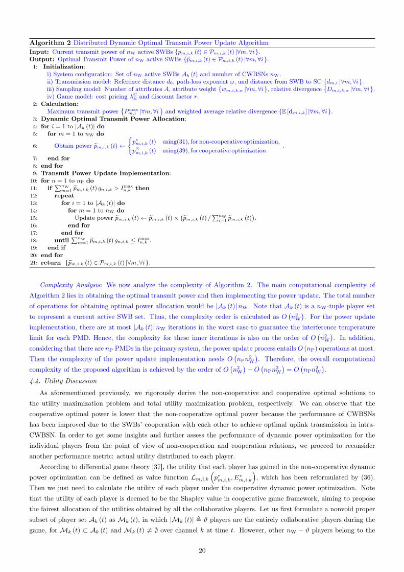
Based on the outcome of Theorem 1 and Theorem 2 obtained above, we present a distributed dynamic optimaltransmit power update algorithm to jointly realize the dynamic optimal transmit power allocation and update imple-mentation, which is sketched in Algorithm 2. The proposed algorithm returns the non-cooperative and cooperativeoptimal power allocation for each SWB on the basis of two dynamic power optimization strategies as its output. First,we initialize and calculate all the necessary parameter values as exactly indicated in the algorithm. Then, we computeand allocate the optimal transmit power in terms of the non-cooperative and cooperative modes according to theproposed differential game theoretic framework. Next, we devise an iteration implementation process to ensure fastconvergence of the update of transmit power. By updating the optimal transmit power for each SWB, the iterationprocess is terminated when the interference temperature limit for each PMD is guaranteed is reached.

19

Algorithm 2 Distributed Dynamic Optimal Transmit Power Update AlgorithmInput: Current transmit power of nW active SWBs {pm,i,k (t) ∈ Pm,i,k (t) |∀m,∀i}.Output: Optimal Transmit Power of nW active SWBs {pm,i,k (t) ∈ Pm,i,k (t) |∀m, ∀i}.1: Initialization:

i) System configuration: Set of nW active SWBs Ak (t) and number of CWBSNs nW.ii) Transmission model: Reference distance d0, path-loss exponent ω, and distance from SWB to SC {dm,i |∀m,∀i}.iii) Sampling model: Number of attributes A, attribute weight {wm,i,k,α |∀m,∀i}, relative divergence {Dm,i,k,α |∀m, ∀i}.iv) Game model: cost pricing λC

E and discount factor r.2: Calculation:

Maximum transmit power{Pmaxm,i |∀m,∀i

}and weighted average relative divergence {E [dm,i,k] |∀m,∀i}.

3: Dynamic Optimal Transmit Power Allocation:4: for i = 1 to |Ak (t)| do5: for m = 1 to nW do

6: Obtain power pm,i,k (t)←

{p∗m,i,k (t) using(31), for non-cooperative optimization,p�m,i,k (t) using(39), for cooperative optimization.

.

7: end for8: end for9: Transmit Power Update Implementation:

10: for n = 1 to nP do11: if

∑nWm=1 pm,i,k (t) gn,i,k > Imax

n,k then12: repeat13: for i = 1 to |Ak (t)| do14: for m = 1 to nW do15: Update power pm,i,k (t)← pm,i,k (t)×

(pm,i,k (t) /

∑nWi=1 pm,i,k (t)

).

16: end for17: end for18: until

∑nWm=1 pm,i,k (t) gn,i,k ≤ I

maxn,k .

19: end if20: end for21: return {pm,i,k (t) ∈ Pm,i,k (t) |∀m,∀i}.

Complexity Analysis: We now analyze the complexity of Algorithm 2. The main computational complexity ofAlgorithm 2 lies in obtaining the optimal transmit power and then implementing the power update. The total numberof operations for obtaining optimal power allocation would be |Ak (t)|nW. Note that Ak (t) is a nW-tuple player setto represent a current active SWB set. Thus, the complexity order is calculated as O

(n2W). For the power update

implementation, there are at most |Ak (t)|nW iterations in the worst case to guarantee the interference temperaturelimit for each PMD. Hence, the complexity for these inner iterations is also on the order of O

(n2W). In addition,

considering that there are nP PMDs in the primary system, the power update process entails O (nP) operations at most.Then the complexity of the power update implementation needs O

(nPn

2W

). Therefore, the overall computational

complexity of the proposed algorithm is achieved by the order of O(n2W)+O

(nPn

2W

)= O

(nPn

2W

).

4.4. Utility Discussion

As aforementioned previously, we rigorously derive the non-cooperative and cooperative optimal solutions tothe utility maximization problem and total utility maximization problem, respectively. We can observe that thecooperative optimal power is lower that the non-cooperative optimal power because the performance of CWBSNshas been improved due to the SWBs’ cooperation with each other to achieve optimal uplink transmission in intra-CWBSN. In order to get some insights and further assess the performance of dynamic power optimization for theindividual players from the point of view of non-cooperation and cooperation relations, we proceed to reconsideranother performance metric: actual utility distributed to each player.

According to differential game theory [37], the utility that each player has gained in the non-cooperative dynamicpower optimization can be defined as value function Lm,i,k

(p∗m,i,k, E

∗m,i,k

), which has been reformulated by (36).

Then we just need to calculate the utility of each player under the cooperative dynamic power optimization. Notethat the utility of each player is deemed to be the Shapley value in cooperative game framework, aiming to proposethe fairest allocation of the utilities obtained by all the collaborative players. Let us first formulate a nonvoid propersubset of player set Ak (t) asMk (t), in which |Mk (t)| , ϑ players are the entirely collaborative players during thegame, for Mk (t) ⊂ Ak (t) and Mk (t) 6= ∅ over channel k at time t. However, other nW − ϑ players belong to the

20

non-cooperative players. In other words, ϑ collaborative players agree to constitute a partial coalitionMk (t) of playerset Ak (t) to play against other nW − ϑ non-cooperative players. The following definition set a formal formulation ofthe Shapley value that is used to distribute the total cooperative utilities to the collaborative players.

Definition 3. (Shapley Value) The Shapley value Om,i,k(p�m,i,k, E

�m,i,k

)for SWB i in CWBSN m over channel k

under the cooperative dynamic power optimization can be mathematically defined as:

Om,i,k(p�m,i,k, E

�m,i,k

)=

∑i∈Mk(t)

(n− ϑ)! (ϑ− 1)!

n!(Wm,i,k (Mk (t))−Wm,i,k (Mk (t) \ {i})) , (44)

where Wm,i,k (Mk (t)) is the predefined value function of the cooperative dynamic power optimization under partialcoalition Mk (t), and Wm,i,k (Mk (t) \ {i}) = Lm,i,k

(p∗m,i,k, E

∗m,i,k

)is the derived value function exploited by the

non-cooperative dynamic power optimization.

With this definition, we need to provide a theoretical derivation of the predefined value function to calculate theShapley value. Notice that the partial coalitionMk (t) refers to a partially cooperative scenario that ϑ players agreeto cooperate in contrast to a fully cooperative scenario that nW players make joint strategies via full cooperationamong those players. Under this scenario, let us build a dynamic programming formulation to derive an optimalsolution to the cooperative dynamic power optimization under partial coalition Mk (t). In this formulation, ourtarget is to maximize the total utilities of all SWBs belonging to the partial coalitionMk (t) throughout time interval[t′0, t0 +DSlot] while satisfying the constraints (27b)-(27d), which can be precisely expressed as:

maximize{pm,i,k(t)},{Em,i,k(t)}

∑i∈Mk(t)

∫ t0+DSlot

t′0

(λRm,i,k

(Pmaxm,i − pm,i,k (t)

)− λCE

Em,i,k (t)

tT

)e−r(t−t

′0)dt (45a)

subject to (27b), (27c), (27d), (45b)

pm,j,k (t) = p∗m,j,k (t) ,∀j ∈ NW \Mk (t) , (45c)

where constraint (45c) indicates that the optimal power values of other nW− |Mk (t)| non-cooperative players shouldbe represented by the non-cooperative optimal power in (31). Let pMk(t)

m,i,k (t) and EMk(t)m,i,k (t) denote the cooperative

optimal transmit power and energy consumption for SWB i in CWBSN m over channel k under partial coalitionMk (t), respectively. Invoking Pontryagin’s maximum principle, we also assume that there exists a continuouslydifferentiable auxiliary value function Wm,i,k (Mk (t)) satisfying the partial differential equation given as follows [37]:

rWm,i,k (Mk (t))

= max{pm,i,k(t)},{Em,i,k(t)}

∑i∈Mk(t)

(λRm,i,k

(Pmaxm,i − pm,i,k (t)

)− λCE

Em,i,k (t)

tT

)

+∂Wm,i,k (Mk (t))

∂Em,i,k (t)

(ERm,i,k (t)− tTpm,i,k (t)− Em,i,k (t)

)}. (46)

Theorem 3. The cooperative optimal transmit power pMk(t)m,i,k (t) constitutes the cooperative optimal solution to the

total utility maximization problem in (45) if and only if the cooperative optimal transmit power pMk(t)m,i,k (t) and the

value function Wm,i,k (Mk (t)) can be formulated as:

pMk(t)m,i,k (t) = Pmax

m,i

(1− ϑλCE

2 (r + 1)E [dm,i,k]

), (47)

Wm,i,k (Mk (t)) = −ϑλCE

tT (r + 1). (48)

21

Proof : The proof of the theorem is similar to that of Theorem 2, and thus is omitted due to space limitations.

We now claim that the optimal power of all players including partial coalition Mk (t) and other nW − ϑ non-cooperative players can be determined as follows:

Pmaxm,1

(1− ϑλCE

2(r+1)E[dm,1,k]

),··· ,Pmax

m,ϑ

(1− ϑλCE

2(r+1)E[dm,ϑ,k]

)︸ ︷︷ ︸

ϑCollaborative Players

, Pmaxm,ϑ+1

(1− λCE

2(r+1)E[dm,ϑ+1,k]

),··· ,Pmax

m,nW

(1− λCE

2(r+1)E[dm,nW,k]

)︸ ︷︷ ︸

nW−ϑNon-cooperative Players

. (49)

Similarly, we can also say that the cooperative optimal energy consumption EMk(t)m,i,k (t) follows that:

EMk(t)m,i,k (t) = ξ3e

t − ERm,i,k (t) + tTP

maxm,i

(1− ϑλCE

2 (r + 1)E [dm,i,k]

), (50)

where ξ3 is the constant number. On substituting (50) and the results of Theorem 3 into (46), with the aid of somealgebraic manipulations, we can rewrite:

Wm,i,k (Mk (t)) =

(ϑλCE

)24r (r + 1)

2

∑i∈Mk(t)

Pmaxm,i

E [dm,i,k]

−λCE

r

∑i∈Mk(t)

(Pmaxm,i

(1− ϑλCE

2 (r + 1)E [dm,i,k]− ER

m,i,k (t)

))

− ϑλCEξ3tT (r + 1)

et−2ϑλCE

(ERm,i,k (t)− tTPmax

m,i

)tT (r + 1)

−(ϑλCE

)2Pmaxm,i

r (r + 1)2 E [dm,i,k]

. (51)

Applying the value functions given by (51) and (36) into (44), by direct computation, we immediately has theShapley value under the cooperative dynamic power optimization. It is evident that the expression of the Shapleyvalue seems too complicated. For ease of discussion, let us consider a simplified scenario with nW = 3 players denotedby NW = {1, 2, 3} to play the game, and the partial coalition comprises ϑ = 2 players denoted by Mk (t) = {1, 2}.Under the above setting, the corresponding Shapley value can be exactly reformulated as follows:

Om,i,k(p�m,i,k, E

�m,i,k

)=

∑i∈{1,2}

(3− 2)! (2− 1)!

3!

(Wm,i,k (Mk (t))− Lm,i,k

(p∗m,i,k, E

∗m,i,k

))

=1

6

(λCE)2

r (r + 1)2

∑i∈{1,2}

Pmaxm,i

E [dm,i,k]−(λCE)2r

∑i∈{1,2}

(Pmaxm,i

(1− λCE

(r + 1)E [dm,i,k]−ER

m,i,k (t)

))

+3λCE − 16 (r + 1)λCEP

maxm,i

4r (r + 1)E [dm,i,k]−λCE (2r + 1) et + 2λCE

(ERm,i,k (t)− tTPmax

m,i

)tTr (r + 1)

. (52)

Finally, we are then ready to compare the utilities between the non-cooperative and cooperative dynamic poweroptimization to evaluate the performance of dynamic power optimization from the perspective of non-cooperation andcooperation relations. For simplicity, let us define ξ1 = ξ3 = 1. From our previous calculations in (52), we deducethat:

Om,i,k(p�m,i,k, E

�m,i,k

)− Lm,i,k

(p∗m,i,k, E

∗m,i,k

)22

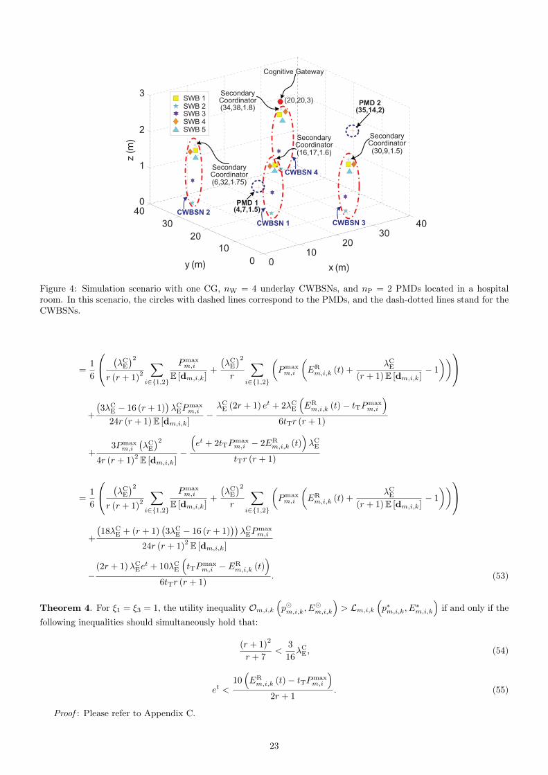
Figure 4: Simulation scenario with one CG, nW = 4 underlay CWBSNs, and nP = 2 PMDs located in a hospitalroom. In this scenario, the circles with dashed lines correspond to the PMDs, and the dash-dotted lines stand for theCWBSNs.

=1

6

(λCE)2

r (r + 1)2

∑i∈{1,2}

Pmaxm,i

E [dm,i,k]+

(λCE)2r

∑i∈{1,2}

(Pmaxm,i

(ERm,i,k (t) +

λCE(r + 1)E [dm,i,k]

− 1

))

+

(3λCE − 16 (r + 1)

)λCEP

maxm,i

24r (r + 1)E [dm,i,k]−λCE (2r + 1) et + 2λCE

(ERm,i,k (t)− tTPmax

m,i

)6tTr (r + 1)

+3Pmax

m,i

(λCE)2

4r (r + 1)2 E [dm,i,k]

−

(et + 2tTP

maxm,i − 2ER

m,i,k (t))λCE

tTr (r + 1)

=1

6

(λCE)2

r (r + 1)2

∑i∈{1,2}

Pmaxm,i

E [dm,i,k]+

(λCE)2r

∑i∈{1,2}

(Pmaxm,i

(ERm,i,k (t) +

λCE(r + 1)E [dm,i,k]

− 1

))+

(18λCE + (r + 1)

(3λCE − 16 (r + 1)

))λCEP

maxm,i

24r (r + 1)2 E [dm,i,k]

−(2r + 1)λCEe

t + 10λCE

(tTP

maxm,i − ER

m,i,k (t))

6tTr (r + 1). (53)

Theorem 4. For ξ1 = ξ3 = 1, the utility inequality Om,i,k(p�m,i,k, E

�m,i,k

)> Lm,i,k

(p∗m,i,k, E

∗m,i,k

)if and only if the

following inequalities should simultaneously hold that:

(r + 1)2

r + 7<

3

16λCE, (54)

et <10(ERm,i,k (t)− tTPmax

m,i

)2r + 1

. (55)

Proof : Please refer to Appendix C.

23

Table 4: The predefined location points of the SWBs for every CWBSN in simulation scenario.

SWB locationLocation point in the three-dimensional space (m)

SWB 1 SWB 2 SWB 3 SWB 4 SWB 5

CWBSN 1 (16.25, 17.00, 1.45) (15.17, 16.75, 0.14) (15.74, 17.41, 0.68) (15.67, 16.83, 1.49) (15.79, 16.82, 1.25)

CWBSN 2 (6.25, 32.22, 1.58) (5.74, 32.12, 0.17) (5.79, 31.61, 0.75) (5.58, 31.97, 1.67) (6.38, 32.19, 1.55)

CWBSN 3 (30.25, 9.26, 1.36) (29.02, 8.52, 0.12) (29.40, 9.18, 0.49) (30.38, 8.88, 1.34) (30.17, 9.38, 1.15)

CWBSN 4 (34.12, 38.47, 1.69) (33.40, 37.18, 0.18) (33.73, 38.46, 0.62) (34.56, 37.83, 1.73) (34.39, 38.27, 1.44)

Table 5: The relative divergence between the approximate probability distribution and the statistical probabilitydistribution as well as the weighted average relative divergence used in the simulations.

Type AttributeRelative divergence Weighted average relative divergence

CWBSN 1 CWBSN 2 CWBSN 3 CWBSN 4 CWBSN 1 CWBSN 2 CWBSN 3 CWBSN 4

SWB 1Attribute 1 0.1095 0.0753 0.0136 0.0528

0.1002 0.0478 0.0370 0.0389Attribute 2 0.1761 0.0713 0.0349 0.0388Attribute 3 0.0362 0.0094 0.0563 0.0287

SWB 2Attribute 1 0.3698 0.0933 0.0217 0.1547

0.1700 0.1553 0.0554 0.0984Attribute 2 0.1124 0.1617 0.0708 0.1289Attribute 3 0.0633 0.1969 0.0691 0.0332

SWB 3Attribute 1 0.1414 0.0271 0.1235 0.0687

0.1175 0.1012 0.0668 0.0588Attribute 2 0.0770 0.0392 0.0862 0.1147Attribute 3 0.1299 0.2033 0.0096 0.0095

SWB 4Attribute 1 0.4508 0.1978 0.1023 0.0228

0.3164 0.1358 0.1462 0.0673Attribute 2 0.1588 0.0692 0.0900 0.1143Attribute 3 0.3337 0.1394 0.2212 0.0656

SWB 5Attribute 1 0.2441 0.0848 0.0560 0.0336

0.1042 0.0826 0.0456 0.0347Attribute 2 0.0282 0.1309 0.0438 0.0308Attribute 3 0.0564 0.0448 0.0392 0.0384

We wish to remark that Theorem 4 provides the fundamental condition that the utility of cooperative scenario islarger than that of competitive scenario according to the actual behaviors of players in the proposed game framework.In summary, we further conclude that the performance of the cooperative dynamic power optimization is better thanthat of the non-cooperative dynamic power optimization from two aspects: the optimal power and the actual utilitygained by each player.

5. Simulation Results

5.1. Simulation Setup

In this section, we present the simulation results to verify our theoretical analysis and evaluate the performance ofour proposed optimization framework under a given system configuration. As depicted in Fig. 4, the simulations areconducted on a hospital room scenario within a three-dimensional space of 40m × 40m × 3m. In this scenario, oneCG and nW = 4 underlay CWBSNs coexist with a primary system consisting of nP = 2 PMDs in a hospital room.More precisely, the CG is deployed on the center of the roof, i.e., the three-dimensional spatial point (20, 20, 3)m. Thelocation points of the near-body SCs are initialized as (16, 17, 1.6)m, (6, 32, 1.75)m, (30, 9, 1.5)m, and (34, 38, 1.8)m,for CWBSN 1, CWBSN 2, CWBSN 3, and CWBSN 4, respectively. Each CWBSN contains nS = 5 SWBs whichare identified from SWB 1 to SWB 5 with different colors and marker, to monitor EEG, foot pressure, EMG, res-piration, and blood pressure, respectively. The predefined location points of the SWBs for every CWBSN in thethree-dimensional space are listed in Table 4. Moreover, the locations of two PMDs marked by PMD 1 and PMD2 are assumed to be set at the location points (4, 7, 1.5)m and (35, 14, 2)m, respectively. We would like to mentionthat our proposed optimization framework is conducted within this given simulation configuration, which can beinterpreted as a specific predefined scenario with limited network nodes due to the space limitations. However, theresults about this framework will be easily extendable to the general case for increased density of nodes.

24

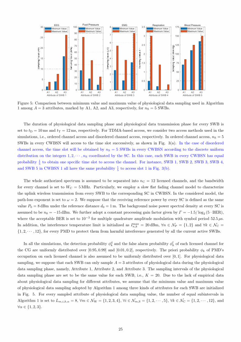
Figure 5: Comparison between minimum value and maximum value of physiological data sampling used in Algorithm1 among A = 3 attributes, marked by A1, A2, and A3, respectively, for nS = 5 SWBs.

The duration of physiological data sampling phase and physiological data transmission phase for every SWB isset to tD = 10ms and tT = 12ms, respectively. For TDMA-based access, we consider two access methods used in thesimulations, i.e., ordered channel access and disordered channel access, respectively. In ordered channel access, nS = 5

SWBs in every CWBSN will access to the time slot successively, as shown in Fig. 3(a). In the case of disorderedchannel access, the time slot will be obtained by nS = 5 SWBs in every CWBSN according to the discrete uniformdistribution on the integers 1, 2, · · · , nS coordinated by the SC. In this case, each SWB in every CWBSN has equalprobability 1

5 to obtain one specific time slot to access the channel. For instance, SWB 1, SWB 2, SWB 3, SWB 4,and SWB 5 in CWBSN 1 all have the same probability 1

5 to access slot 1 in Fig. 3(b).

The whole authorized spectrum is assumed to be separated into nC = 12 licensed channels, and the bandwidthfor every channel is set to WC = 5MHz. Particularly, we employ a slow flat fading channel model to characterizethe uplink wireless transmission from every SWB to the corresponding SC in CWBSN. In the considered model, thepath-loss exponent is set to ω = 2. We suppose that the receiving reference power by every SC is defined as the samevalue P0 = 8dBm under the reference distance d0 = 1m. The background noise power spectral density at every SC isassumed to be n0 = −15 dBm. We further adopt a constant processing gain factor given by Γ = −1.5/ log2 (5 · BER),where the acceptable BER is set to 10−3 for multiple quadrature amplitude modulation with symbol period 52.5µs.In addition, the interference temperature limit is initialized as Imax

n,k = 20dBm, ∀n ∈ NP = {1, 2} and ∀k ∈ NC =

{1, 2, · · · , 12}, for every PMD to protect them from harmful interference generated by all the current active SWBs.

In all the simulations, the detection probability φdk and the false alarm probability φfk of each licensed channel forthe CG are uniformly distributed over [0.95, 0.99] and [0.01, 0.2], respectively. The priori probability φk of PMD’soccupation on each licensed channel is also assumed to be uniformly distributed over [0, 1]. For physiological datasampling, we suppose that each SWB can only sample A = 3 attributes of physiological data during the physiologicaldata sampling phase, namely, Attribute 1, Attribute 2, and Attribute 3. The sampling intervals of the physiologicaldata sampling phase are set to be the same value for each SWB, i.e., K = 20. Due to the lack of empirical dataabout physiological data sampling for different attributes, we assume that the minimum value and maximum valueof physiological data sampling adopted by Algorithm 1 among three kinds of attributes for each SWB are initializedin Fig. 5. For every sampled attribute of physiological data sampling value, the number of equal subintervals inAlgorithm 1 is set to Lm,i,k,α = 8, ∀m ∈ NW = {1, 2, 3, 4}, ∀i ∈ Nm,S = {1, 2, · · · , 5}, ∀k ∈ NC = {1, 2, · · · , 12}, and∀α ∈ {1, 2, 3}.

25

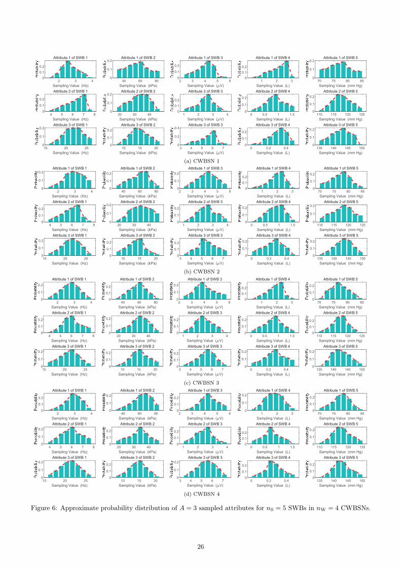
(a) CWBSN 1

(b) CWBSN 2

(c) CWBSN 3

(d) CWBSN 4

Figure 6: Approximate probability distribution of A = 3 sampled attributes for nS = 5 SWBs in nW = 4 CWBSNs.

26

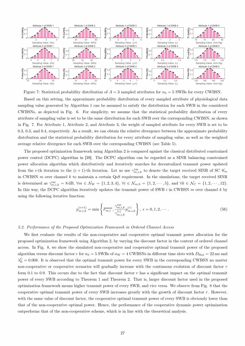
Figure 7: Statistical probability distribution of A = 3 sampled attributes for nS = 5 SWBs for every CWBSN.

Based on this setting, the approximate probability distribution of every sampled attribute of physiological datasampling value generated by Algorithm 1 can be assumed to satisfy the distribution for each SWB in the consideredCWBSNs, as depicted in Fig. 6. For simplicity, we assume that the statistical probability distribution of everyattribute of sampling value is set to be the same distribution for each SWB over the corresponding CWBSN, as shownin Fig. 7. For Attribute 1, Attribute 2, and Attribute 3, the weight of sampled attribute for every SWB is set to be0.3, 0.3, and 0.4, respectively. As a result, we can obtain the relative divergence between the approximate probabilitydistribution and the statistical probability distribution for every attribute of sampling value, as well as the weightedaverage relative divergence for each SWB over the corresponding CWBSN (see Table 5).

The proposed optimization framework using Algorithm 2 is compared against the classical distributed constrainedpower control (DCPC) algorithm in [39]. The DCPC algorithm can be regarded as a SINR balancing constrainedpower allocation algorithm which distributively and iteratively searches for decentralized transmit power updatedfrom the ε-th iteration to the (ε+ 1)-th iteration. Let us use γtar

m,i,k to denote the target received SINR of SC Cm

in CWBSN m over channel k to maintain a certain QoS requirement. In the simulations, the target received SINRis determined as γtar

m,i,k = 8dB, ∀m ∈ NW = {1, 2, 3, 4}, ∀i ∈ Nm,S = {1, 2, · · · , 5}, and ∀k ∈ NC = {1, 2, · · · , 12}.In this way, the DCPC algorithm iteratively updates the transmit power of SWB i in CWBSN m over channel k byusing the following iterative function:

p(ε+1)m,i,k = min

{Pmaxm,i ,

γtarm,i,k

γ(ε)m,i,k

p(ε)m,i,k

}, ε = 0, 1, 2, · · · . (56)

5.2. Performance of the Proposed Optimization Framework in Ordered Channel Access

We first evaluate the results of the non-cooperative and cooperative optimal transmit power allocation for theproposed optimization framework using Algorithm 2, by varying the discount factor in the context of ordered channelaccess. In Fig. 8, we show the simulated non-cooperative and cooperative optimal transmit power of the proposedalgorithm versus discount factor r for nS = 5 SWBs of nW = 4 CWBSNs in different time slots with DSlot = 22ms andλCE = 0.008. It is observed that the optimal transmit power for every SWB in the corresponding CWBSN no matternon-cooperative or cooperative scenarios will gradually increase with the continuous evolution of discount factor rform 0.1 to 0.9. This occurs due to the fact that discount factor r has a significant impact on the optimal transmitpower of every SWB according to Theorem 1 and Theorem 2. That is, larger discount factor used in the proposedoptimization framework means higher transmit power of every SWB, and vice versa. We observe from Fig. 8 that thecooperative optimal transmit power of every SWB increases greatly with the growth of discount factor r. However,with the same value of discount factor, the cooperative optimal transmit power of every SWB is obviously lower thanthat of the non-cooperative optimal power. Hence, the performance of the cooperative dynamic power optimizationoutperforms that of the non-cooperative scheme, which is in line with the theoretical analysis.

27

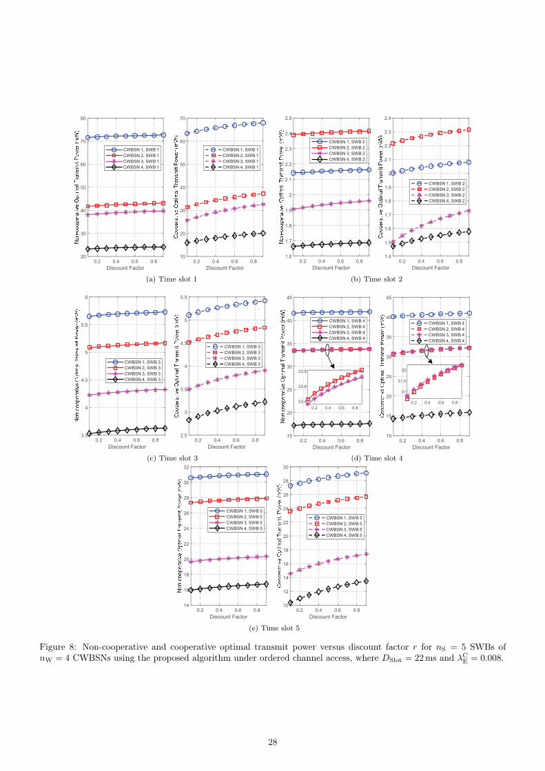
(a) Time slot 1 (b) Time slot 2

(c) Time slot 3 (d) Time slot 4

(e) Time slot 5

Figure 8: Non-cooperative and cooperative optimal transmit power versus discount factor r for nS = 5 SWBs ofnW = 4 CWBSNs using the proposed algorithm under ordered channel access, where DSlot = 22ms and λCE = 0.008.

28

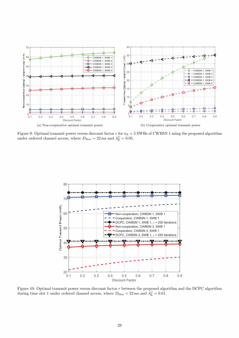
(a) Non-cooperative optimal transmit power (b) Cooperative optimal transmit power

Figure 9: Optimal transmit power versus discount factor r for nS = 5 SWBs of CWBSN 1 using the proposed algorithmunder ordered channel access, where DSlot = 22ms and λCE = 0.05.

Figure 10: Optimal transmit power versus discount factor r between the proposed algorithm and the DCPC algorithmduring time slot 1 under ordered channel access, where DSlot = 22ms and λCE = 0.01.

29

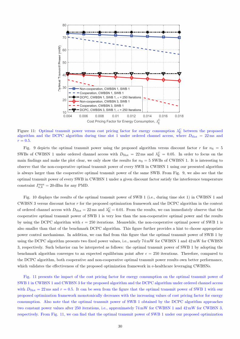
Figure 11: Optimal transmit power versus cost pricing factor for energy consumption λCE between the proposedalgorithm and the DCPC algorithm during time slot 1 under ordered channel access, where DSlot = 22ms andr = 0.5.

Fig. 9 depicts the optimal transmit power using the proposed algorithm versus discount factor r for nS = 5

SWBs of CWBSN 1 under ordered channel access with DSlot = 22ms and λCE = 0.05. In order to focus on themain findings and make the plot clear, we only show the results for nS = 5 SWBs of CWBSN 1. It is interesting toobserve that the non-cooperative optimal transmit power of every SWB in CWBSN 1 using our presented algorithmis always larger than the cooperative optimal transmit power of the same SWB. From Fig. 9, we also see that theoptimal transmit power of every SWB in CWBSN 1 under a given discount factor satisfy the interference temperatureconstraint Imax

n,k = 20dBm for any PMD.

Fig. 10 displays the results of the optimal transmit power of SWB 1 (i.e., during time slot 1) in CWBSN 1 andCWBSN 3 versus discount factor r for the proposed optimization framework and the DCPC algorithm in the contextof ordered channel access with DSlot = 22ms and λCE = 0.01. From the results, we can immediately observe that thecooperative optimal transmit power of SWB 1 is very less than the non-cooperative optimal power and the resultsby using the DCPC algorithm with ε = 250 iterations. Meanwhile, the non-cooperative optimal power of SWB 1 isalso smaller than that of the benchmark DCPC algorithm. This figure further provides a hint to choose appropriatepower control mechanisms. In addition, we can find from this figure that the optimal transmit power of SWB 1 byusing the DCPC algorithm presents two fixed power values, i.e., nearly 74mW for CWBSN 1 and 42mW for CWBSN3, respectively. Such behavior can be interpreted as follows: the optimal transmit power of SWB 1 by adopting thebenchmark algorithm converges to an expected equilibrium point after ε = 250 iterations. Therefore, compared tothe DCPC algorithm, both cooperative and non-cooperative optimal transmit power results own better performance,which validates the effectiveness of the proposed optimization framework in e-healthcare leveraging CWBSNs.

Fig. 11 presents the impact of the cost pricing factor for energy consumption on the optimal transmit power ofSWB 1 in CWBSN 1 and CWBSN 3 for the proposed algorithm and the DCPC algorithm under ordered channel accesswith DSlot = 22ms and r = 0.5. It can be seen from the figure that the optimal transmit power of SWB 1 with ourproposed optimization framework monotonically decreases with the increasing values of cost pricing factor for energyconsumption. Also note that the optimal transmit power of SWB 1 obtained by the DCPC algorithm approachestwo constant power values after 250 iterations, i.e., approximately 74mW for CWBSN 1 and 42mW for CWBSN 3,respectively. From Fig. 11, we can find that the optimal transmit power of SWB 1 under our proposed optimization

30

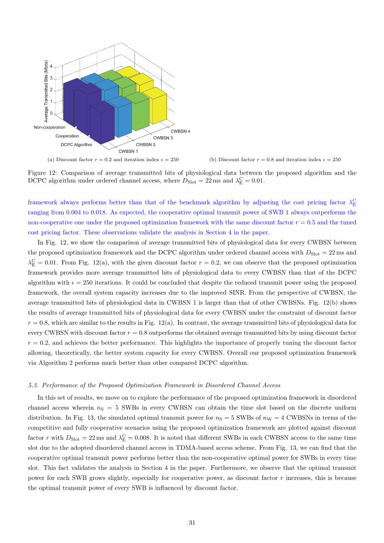
(a) Discount factor r = 0.2 and iteration index ε = 250 (b) Discount factor r = 0.8 and iteration index ε = 250

Figure 12: Comparison of average transmitted bits of physiological data between the proposed algorithm and theDCPC algorithm under ordered channel access, where DSlot = 22ms and λCE = 0.01.

framework always performs better than that of the benchmark algorithm by adjusting the cost pricing factor λCEranging from 0.004 to 0.018. As expected, the cooperative optimal transmit power of SWB 1 always outperforms thenon-cooperative one under the proposed optimization framework with the same discount factor r = 0.5 and the tunedcost pricing factor. These observations validate the analysis in Section 4 in the paper.

In Fig. 12, we show the comparison of average transmitted bits of physiological data for every CWBSN betweenthe proposed optimization framework and the DCPC algorithm under ordered channel access with DSlot = 22ms andλCE = 0.01. From Fig. 12(a), with the given discount factor r = 0.2, we can observe that the proposed optimizationframework provides more average transmitted bits of physiological data to every CWBSN than that of the DCPCalgorithm with ε = 250 iterations. It could be concluded that despite the reduced transmit power using the proposedframework, the overall system capacity increases due to the improved SINR. From the perspective of CWBSN, theaverage transmitted bits of physiological data in CWBSN 1 is larger than that of other CWBSNs. Fig. 12(b) showsthe results of average transmitted bits of physiological data for every CWBSN under the constraint of discount factorr = 0.8, which are similar to the results in Fig. 12(a). In contrast, the average transmitted bits of physiological data forevery CWBSN with discount factor r = 0.8 outperforms the obtained average transmitted bits by using discount factorr = 0.2, and achieves the better performance. This highlights the importance of properly tuning the discount factorallowing, theoretically, the better system capacity for every CWBSN. Overall our proposed optimization frameworkvia Algorithm 2 performs much better than other compared DCPC algorithm.

5.3. Performance of the Proposed Optimization Framework in Disordered Channel Access

In this set of results, we move on to explore the performance of the proposed optimization framework in disorderedchannel access wherein nS = 5 SWBs in every CWBSN can obtain the time slot based on the discrete uniformdistribution. In Fig. 13, the simulated optimal transmit power for nS = 5 SWBs of nW = 4 CWBSNs in terms of thecompetitive and fully cooperative scenarios using the proposed optimization framework are plotted against discountfactor r with DSlot = 22ms and λCE = 0.008. It is noted that different SWBs in each CWBSN access to the same timeslot due to the adopted disordered channel access in TDMA-based access scheme. From Fig. 13, we can find that thecooperative optimal transmit power performs better than the non-cooperative optimal power for SWBs in every timeslot. This fact validates the analysis in Section 4 in the paper. Furthermore, we observe that the optimal transmitpower for each SWB grows slightly, especially for cooperative power, as discount factor r increases, this is becausethe optimal transmit power of every SWB is influenced by discount factor.

31

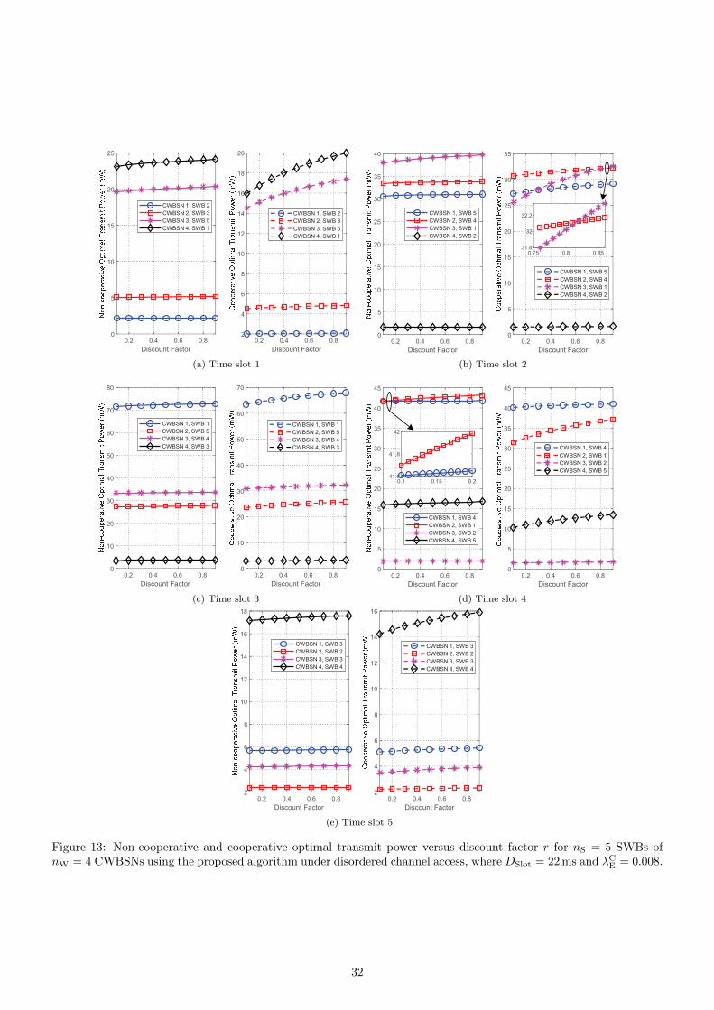
(a) Time slot 1 (b) Time slot 2

(c) Time slot 3 (d) Time slot 4

(e) Time slot 5

Figure 13: Non-cooperative and cooperative optimal transmit power versus discount factor r for nS = 5 SWBs ofnW = 4 CWBSNs using the proposed algorithm under disordered channel access, where DSlot = 22ms and λCE = 0.008.

32

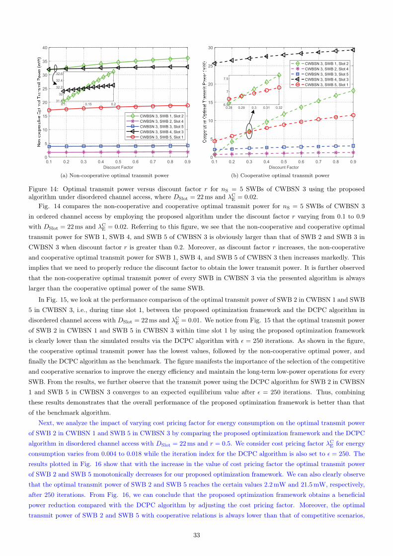
(a) Non-cooperative optimal transmit power (b) Cooperative optimal transmit power

Figure 14: Optimal transmit power versus discount factor r for nS = 5 SWBs of CWBSN 3 using the proposedalgorithm under disordered channel access, where DSlot = 22ms and λCE = 0.02.

Fig. 14 compares the non-cooperative and cooperative optimal transmit power for nS = 5 SWBs of CWBSN 3in ordered channel access by employing the proposed algorithm under the discount factor r varying from 0.1 to 0.9

with DSlot = 22ms and λCE = 0.02. Referring to this figure, we see that the non-cooperative and cooperative optimaltransmit power for SWB 1, SWB 4, and SWB 5 of CWBSN 3 is obviously larger than that of SWB 2 and SWB 3 inCWBSN 3 when discount factor r is greater than 0.2. Moreover, as discount factor r increases, the non-cooperativeand cooperative optimal transmit power for SWB 1, SWB 4, and SWB 5 of CWBSN 3 then increases markedly. Thisimplies that we need to properly reduce the discount factor to obtain the lower transmit power. It is further observedthat the non-cooperative optimal transmit power of every SWB in CWBSN 3 via the presented algorithm is alwayslarger than the cooperative optimal power of the same SWB.

In Fig. 15, we look at the performance comparison of the optimal transmit power of SWB 2 in CWBSN 1 and SWB5 in CWBSN 3, i.e., during time slot 1, between the proposed optimization framework and the DCPC algorithm indisordered channel access with DSlot = 22ms and λCE = 0.01. We notice from Fig. 15 that the optimal transmit powerof SWB 2 in CWBSN 1 and SWB 5 in CWBSN 3 within time slot 1 by using the proposed optimization frameworkis clearly lower than the simulated results via the DCPC algorithm with ε = 250 iterations. As shown in the figure,the cooperative optimal transmit power has the lowest values, followed by the non-cooperative optimal power, andfinally the DCPC algorithm as the benchmark. The figure manifests the importance of the selection of the competitiveand cooperative scenarios to improve the energy efficiency and maintain the long-term low-power operations for everySWB. From the results, we further observe that the transmit power using the DCPC algorithm for SWB 2 in CWBSN1 and SWB 5 in CWBSN 3 converges to an expected equilibrium value after ε = 250 iterations. Thus, combiningthese results demonstrates that the overall performance of the proposed optimization framework is better than thatof the benchmark algorithm.

Next, we analyze the impact of varying cost pricing factor for energy consumption on the optimal transmit powerof SWB 2 in CWBSN 1 and SWB 5 in CWBSN 3 by comparing the proposed optimization framework and the DCPCalgorithm in disordered channel access with DSlot = 22ms and r = 0.5. We consider cost pricing factor λCE for energyconsumption varies from 0.004 to 0.018 while the iteration index for the DCPC algorithm is also set to ε = 250. Theresults plotted in Fig. 16 show that with the increase in the value of cost pricing factor the optimal transmit powerof SWB 2 and SWB 5 monotonically decreases for our proposed optimization framework. We can also clearly observethat the optimal transmit power of SWB 2 and SWB 5 reaches the certain values 2.2mW and 21.5mW, respectively,after 250 iterations. From Fig. 16, we can conclude that the proposed optimization framework obtains a beneficialpower reduction compared with the DCPC algorithm by adjusting the cost pricing factor. Moreover, the optimaltransmit power of SWB 2 and SWB 5 with cooperative relations is always lower than that of competitive scenarios,

33

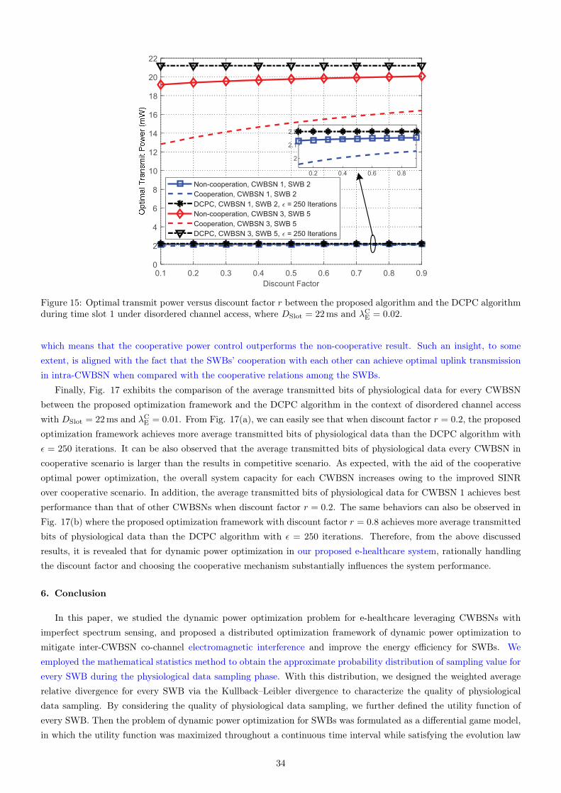
Figure 15: Optimal transmit power versus discount factor r between the proposed algorithm and the DCPC algorithmduring time slot 1 under disordered channel access, where DSlot = 22ms and λCE = 0.02.

which means that the cooperative power control outperforms the non-cooperative result. Such an insight, to someextent, is aligned with the fact that the SWBs’ cooperation with each other can achieve optimal uplink transmissionin intra-CWBSN when compared with the cooperative relations among the SWBs.

Finally, Fig. 17 exhibits the comparison of the average transmitted bits of physiological data for every CWBSNbetween the proposed optimization framework and the DCPC algorithm in the context of disordered channel accesswith DSlot = 22ms and λCE = 0.01. From Fig. 17(a), we can easily see that when discount factor r = 0.2, the proposedoptimization framework achieves more average transmitted bits of physiological data than the DCPC algorithm withε = 250 iterations. It can be also observed that the average transmitted bits of physiological data every CWBSN incooperative scenario is larger than the results in competitive scenario. As expected, with the aid of the cooperativeoptimal power optimization, the overall system capacity for each CWBSN increases owing to the improved SINRover cooperative scenario. In addition, the average transmitted bits of physiological data for CWBSN 1 achieves bestperformance than that of other CWBSNs when discount factor r = 0.2. The same behaviors can also be observed inFig. 17(b) where the proposed optimization framework with discount factor r = 0.8 achieves more average transmittedbits of physiological data than the DCPC algorithm with ε = 250 iterations. Therefore, from the above discussedresults, it is revealed that for dynamic power optimization in our proposed e-healthcare system, rationally handlingthe discount factor and choosing the cooperative mechanism substantially influences the system performance.

6. Conclusion

In this paper, we studied the dynamic power optimization problem for e-healthcare leveraging CWBSNs withimperfect spectrum sensing, and proposed a distributed optimization framework of dynamic power optimization tomitigate inter-CWBSN co-channel electromagnetic interference and improve the energy efficiency for SWBs. Weemployed the mathematical statistics method to obtain the approximate probability distribution of sampling value forevery SWB during the physiological data sampling phase. With this distribution, we designed the weighted averagerelative divergence for every SWB via the Kullback–Leibler divergence to characterize the quality of physiologicaldata sampling. By considering the quality of physiological data sampling, we further defined the utility function ofevery SWB. Then the problem of dynamic power optimization for SWBs was formulated as a differential game model,in which the utility function was maximized throughout a continuous time interval while satisfying the evolution law

34

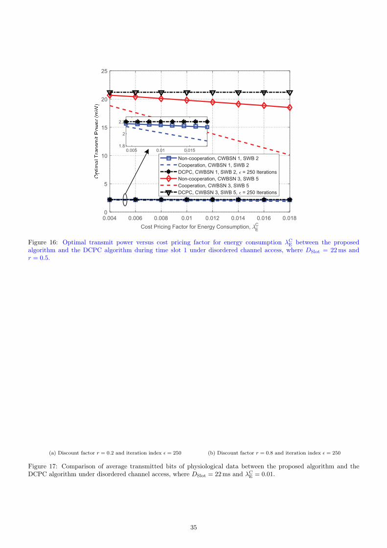
Figure 16: Optimal transmit power versus cost pricing factor for energy consumption λCE between the proposedalgorithm and the DCPC algorithm during time slot 1 under disordered channel access, where DSlot = 22ms andr = 0.5.

(a) Discount factor r = 0.2 and iteration index ε = 250 (b) Discount factor r = 0.8 and iteration index ε = 250

Figure 17: Comparison of average transmitted bits of physiological data between the proposed algorithm and theDCPC algorithm under disordered channel access, where DSlot = 22ms and λCE = 0.01.

35

of energy consumption in the battery of every SWB. From the perspective of the non-cooperation and cooperationrelations for SWBs, we converted the game model into two subproblems, namely, utility maximization problem andtotal utility maximization problem, and also derived the non-cooperative and cooperative optimal solutions for poweroptimization. We further showed that the performance of the cooperative dynamic power optimization is betterthan that of the non-cooperative optimization in terms of the optimal power and the actual utility gained by eachSWB, respectively. Our simulation results demonstrated the practicality of implementing the proposed optimizationframework to achieve considerable amount of power savings and improved system capacity in e-healthcare scenario.Besides, we showed that better performance can be achieved by using the cooperative mechanism to maximize theoverall utilities rather than the competitive scheme to obtain the individual utility maximization.

Acknowledgments

This work was supported in part by the National Natural Science Foundation of China under Grants 61901115,61971032 and 61802107, the Research Program for Top-notch Young Talents in Higher Education Institutions of HebeiProvince, China under Grant BJ2017037, the Natural Science Foundation of Hebei Province under Grants F2019402206and F2018402198, the Natural Science Foundation of Guangdong Province under Grant 2018A030313492, and theFundamental Research Funds for the Central Universities under Grants FRF-TP-18-008A3 and 328201911.

Appendix A. Proof of Theorem 1

First of all, based on this conversion from the general differential game model Gk into an infinite horizon one, weintend to perform the maximization operation of the right hand side of (30) with respect to the variable pm,i,k (t). Toreach this goal, we obtain the partial derivative of the right hand side of (30) with respect to the variable pm,i,k (t),and give the following indeed solution:

2E [dm,i,k]Pmaxm,i − p∗m,i,k (t)

Pmaxm,i

+∂Lm,i,k

(p∗m,i,k, E

∗m,i,k

)∂E∗m,i,k (t)

, 0. (A.1)

After some simplifications, the non-cooperative optimal solution p∗m,i,k (t) can be obtained by:

p∗m,i,k (t) = Pmaxm,i

1 +tT

2E [dm,i,k]

∂Lm,i,k(p∗m,i,k, E

∗m,i,k

)∂E∗m,i,k (t)

. (A.2)

Substituting (A.2) back into (30), straightforward computation yields that:

Lm,i,k(p∗m,i,k, E

∗m,i,k

)=

Pmaxm,i t

2T

4rE [dm,i,k]

∂Lm,i,k(p∗m,i,k, E

∗m,i,k

)∂E∗m,i,k (t)

2

+ERm,i,k (t)− tTpm,i,k (t)− E∗m,i,k (t)

r

∂Lm,i,k(p∗m,i,k, E

∗m,i,k

)∂E∗m,i,k (t)

. (A.3)

Now we are ready to derive the derivative of value function Lm,i,k(p∗m,i,k, E

∗m,i,k

)with respect to the non-

cooperative optimal energy consumption E∗m,i,k (t) in (A.3). Upon solving the partial differential equation, we canobtain the auxiliary function as the partial differential equation, which can be expressed as:

∂Lm,i,k(p∗m,i,k, E

∗m,i,k

)∂E∗m,i,k (t)

= − λCEtT (r + 1)

. (A.4)

By substituting the expression of value function in (A.4) into (A.2), we can easily obtain the non-cooperativeoptimal solution which is equivalent to:

36

p∗m,i,k (t) = Pmaxm,i

(1− λCE

2 (r + 1)E [dm,i,k]

). (A.5)

which constitutes the NE to the non-cooperative game Gk. This concludes the proof of our theorem.

Appendix B. Proof of Theorem 2

The proof is very similar to that of Theorem 1. The only difference is that the optimization objective of thetotal utility maximization problem in (37) is to maximize the sum of the utility functions of all SWBs. Likewise, inthis appendix, we are also ready to transform the total utility maximization problem in (37) into an infinite horizondifferential game model by relaxing the terminal time t0+DSlot as infinite time horizon. Performing the maximizationoperation of the right hand side of (38) with respect to the variable pm,i,k (t), we have the following result:

p�m,i,k (t) = Pmaxm,i

1 +tT

2E [dm,i,k]

∂Fm,i,k(p�m,i,k, E

�m,i,k

)∂E�m,i,k (t)

. (B.1)

Plugging (B.1) back into (38), after some algebraic manipulations, we immediately have:

Fm,i,k(p�m,i,k, E

�m,i,k

)=t2T4r

nW∑i=1

∂Fm,i,k(p�m,i,k, E

�m,i,k

)∂E�m,i,k (t)

2

−t2TP

maxm,i

2rE [dm,i,k]

∂Fm,i,k(p�m,i,k, E

�m,i,k

)∂E�m,i,k (t)

2

+

(ERm,i,k (t)− tTpm,i,k (t)− E

�m,i,k (t)

)r

·∂Fm,i,k

(p�m,i,k, E

�m,i,k

)∂E�m,i,k (t)

− λCE

rtT

nW∑i=1

E�m,i,k (t) . (B.2)

Following (B.2), we start by deriving the derivative of value function Fm,i,k(p�m,i,k, E

�m,i,k

)with respect to the

cooperative optimal energy consumption E�m,i,k (t) in (41). It is sufficient to prove that∑nW

i=1 λCE = nWλ

CE for each

SWB. Upon solving the partial differential equation, we can immediately obtain the auxiliary function as the partialdifferential equation calculated by (40). By substituting the expression of value function in (40) into (B.1), we caneasily get the cooperative optimal solution as formulated by (39). As a result, Theorem 2 is derived.

Appendix C. Proof of Theorem 4

From the right hand side of (53), we observe that it can be verified that the component 16 (·) since we can exactly

get the following main result: ∑i∈{1,2}

(Pmaxm,i

(ERm,i,k (t) +

λCE(r + 1)E [dm,i,k]

− 1

))

≈∑

i∈{1,2}

(Pmaxm,i

(ERm,i,k (t) +

λCE(r + 1)E [dm,i,k]

)). (C.1)

After a reasonable approximation, it is easily shown that:

∑i∈{1,2}

(Pmaxm,i

(ERm,i,k (t) +

λCE(r + 1)E [dm,i,k]

))> 0. (C.2)

Furthermore, in order to guarantee that Om,i,k(p�m,i,k, E

�m,i,k

)> Lm,i,k

(p∗m,i,k, E

∗m,i,k

), we can also obviously

check that:

37

(18λCE + (r + 1)

(3λCE − 16 (r + 1)

))λCEP

maxm,i > 0,

=⇒ 18λCE +(3λCE − 16 (r + 1)

)(r + 1) > 0,

=⇒ 3λCE (r + 7) > 16 (r + 1)2, (C.3)

and

(2r + 1)λCEet + 10λCE

(tTP

maxm,i − ER

m,i,k (t))< 0,

=⇒ 10(ERm,i,k (t)− tTP

maxm,i

)> (2r + 1) et. (C.4)

For the discount factor 0 < r < 1, it then follows from (C.3) and (C.4) that the inequalities (54) and (55) are bothexactly satisfied. This completes the proof.

References

[1] J. Sun, Y. Fang, X. Zhu, Privacy and emergency response in e-healthcare leveraging wireless body sensor networks,IEEE Wireless Communications 17 (1) (2010) 66–73. doi:10.1109/mwc.2010.5416352.

[2] X. Yang, R. Lu, J. Shao, X. Tang, H. Yang, An efficient and privacy-preserving disease risk prediction schemefor e-healthcare, IEEE Internet of Things Journal 6 (2) (2019) 3284–3297. doi:10.1109/jiot.2018.2882224.

[3] A. M. Rahmani, T. N. Gia, B. Negash, A. Anzanpour, I. Azimi, M. Jiang, P. Liljeberg, Exploiting smart e-healthgateways at the edge of healthcare Internet-of-Things: A fog computing approach, Future Generation ComputerSystems 78 (2018) 641–658. doi:10.1016/j.future.2017.02.014.

[4] X. Yuan, C. Li, Q. Ye, K. Zhang, N. Cheng, N. Zhang, X. Shen, Performance analysis of IEEE 802.15.6-basedcoexisting mobile WBANs with prioritized traffic and dynamic interference, IEEE Transactions on WirelessCommunications 17 (8) (2018) 5637–5652. doi:10.1109/twc.2018.2848223.

[5] S. Movassaghi, M. Abolhasan, J. Lipman, D. Smith, A. Jamalipour, Wireless body area net-works: A survey, IEEE Communications Surveys & Tutorials 16 (3) (Third Quarter 2014) 1658–1686.doi:10.1109/surv.2013.121313.00064.

[6] M. M. Dhanvijay, S. C. Patil, Internet of Things: A survey of enabling technologies in healthcare and its appli-cations, Computer Networks 153 (2019) 113–131. doi:10.1016/j.comnet.2019.03.006.

[7] B. Antonescu, S. Basagni, Wireless body area networks: Challenges, trends and emerging technologies,in: Proc. International Conference on Body Area Networks (BodyNets), Boston, MA, USA, 2013, pp. 1–7.doi:10.4108/icst.bodynets.2013.253722.

[8] P. Phunchongharn, E. Hossain, D. Niyato, S. Camorlinga, A cognitive radio system for e-health applications ina hospital environment, IEEE Wireless Communications 17 (1) (2010) 20–28. doi:10.1109/mwc.2010.5416346.

[9] R. Chavez-Santiago, K. E. Nolan, O. Holland, L. D. Nardis, J. M. Ferro, N. Barroca, L. M. Borges, F. J. Velez,V. Goncalves, I. Balasingham, Cognitive radio for medical body area networks using ultra wideband, IEEEWireless Communications 19 (4) (2012) 74–81. doi:10.1109/mwc.2012.6272426.

[10] M. Naeem, U. Pareek, D. C. Lee, A. S. Khwaja, A. Anpalagan, Wireless resource allocation in next generationhealthcare facilities, IEEE Sensors Journal 15 (3) (2015) 1463–1474. doi:10.1109/jsen.2014.2363571.

[11] S. Sodagari, B. Bozorgchami, H. Aghvami, Technologies and challenges for cognitive radio enabled medical wirelessbody area networks, IEEE Access 6 (2018) 29567–29586. doi:10.1109/access.2018.2843259.

[12] C. Zhang, L. Zhu, C. Xu, R. Lu, PPDP: An efficient and privacy-preserving disease predictionscheme in cloud-based e-Healthcare system, Future Generation Computer Systems 79 (2018) 16–25.doi:10.1016/j.future.2017.09.002.

38

[13] W. Zang, S. Zhang, Y. Li, An accelerometer-assisted transmission power control solution for energy-efficientcommunications in WBAN, IEEE Journal on Selected Areas in Communications 34 (12) (2016) 3427–3437.doi:10.1109/jsac.2016.2611844.

[14] M. Chiang, Balancing transport and physical layers in wireless multihop networks: Jointly optimal conges-tion control and power control, IEEE Journal on Selected Areas in Communications 23 (1) (2005) 104–116.doi:10.1109/jsac.2004.837347.

[15] S. Wang, Z.-H. Zhou, M. Ge, C. Wang, Resource allocation for heterogeneous cognitive radio networks withimperfect spectrum sensing, IEEE Journal on Selected Areas in Communications 31 (3) (2013) 464–475.doi:10.1109/jsac.2013.130312.

[16] H. Zhang, C. Jiang, X. Mao, H.-H. Chen, Interference-limited resource optimization in cognitive femtocells withfairness and imperfect spectrum sensing, IEEE Transactions on Vehicular Technology 65 (3) (2016) 1761–1771.doi:10.1109/tvt.2015.2405538.

[17] S. Kim, D.-S. Eom, Link-state-estimation-based transmission power control in wireless body area networks, IEEEJournal of Biomedical and Health Informatics 18 (4) (2014) 1294–1302. doi:10.1109/jbhi.2013.2282864.

[18] D. Fernandes, A. G. Ferreira, R. Abrishambaf, J. Mendes, J. Cabral, A low traffic overhead trans-mission power control for wireless body area networks, IEEE Sensors Journal 18 (3) (2018) 1301–1313.doi:10.1109/jsen.2017.2778802.

[19] Z. Liu, B. Liu, C. W. Chen, Joint power-rate-slot resource allocation in energy harvesting-poweredwireless body area networks, IEEE Transactions on Vehicular Technology 67 (12) (2018) 12152–12164.doi:10.1109/tvt.2018.2872960.

[20] J. Dong, D. Smith, Joint relay selection and transmit power control for wireless body area networks coexistence,in: Proc. IEEE International Conference on Communications (ICC), Sydney, Australia, 2014, pp. 5676–5681.doi:10.1109/icc.2014.6884226.

[21] Y. Zhang, B. Zhang, A relay-aided transmission power control method in wireless body area networks, IEEEAccess 5 (2017) 8408–8418. doi:10.1109/access.2017.2698158.

[22] G. Chen, Y. Zhan, Y. Chen, L. Xiao, Y. Wang, N. An, Reinforcement learning based power control for in-bodysensors in WBANs against jamming, IEEE Access 6 (2018) 37403–37412. doi:10.1109/access.2018.2850659.

[23] R. Kazemi, R. Vesilo, E. Dutkiewicz, R. Liu, Dynamic power control in wireless body area networks using rein-forcement learning with approximation, in: Proc. IEEE International Symposium on Personal, Indoor and MobileRadio Communications (PIMRC), Toronto, Canada, 2011, pp. 2203–2208. doi:10.1109/pimrc.2011.6139908.

[24] X. Zhao, B. Liu, C. Chen, C. W. Chen, QoS-driven power control for inter-WBAN interference miti-gation, in: Proc. IEEE Global Communications Conference (GLOBECOM), San Diego, CA, USA, 2015.doi:10.1109/glocom.2015.7417058.

[25] Z. Zhang, H. Wang, C. Wang, H. Fang, Interference mitigation for cyber-physical wireless body area networksystem using social networks, IEEE Transactions on Emerging Topics in Computing 1 (1) (2013) 121–132.doi:10.1109/tetc.2013.2274430.

[26] H. Moosavi, F. M. Bui, Optimal relay selection and power control with quality-of-service provisioning inwireless body area networks, IEEE Transactions on Wireless Communications 15 (8) (2016) 5497–5510.doi:10.1109/twc.2016.2560820.

[27] J. Wang, Y. Sun, Y. Ji, QoS-based adaptive power control scheme for co-located WBANs: A cooperative bar-gaining game theoretic perspective, Wireless Networks 24 (8) (2017) 3129–3139. doi:10.1007/s11276-017-1521-2.

[28] Y. Yang, D. B. Smith, Wireless body area networks: Energy-efficient, provably socially-efficient, transmitpower control, in: Proc. IEEE International Conference on Communications (ICC), Paris, France, 2017.doi:10.1109/icc.2017.7997347.

[29] L. Zhang, Z. Zhao, Q. Wu, H. Zhao, H. Xu, X. Wu, Energy-aware dynamic resource allocation inUAV assisted mobile edge computing over social internet of vehicles, IEEE Access 6 (2018) 56700–56715.doi:10.1109/access.2018.2872753.

[30] N. Patwari, A. O. Hero, M. Perkins, N. S. Correal, R. J. O’Dea, Relative location estimation in wireless sensornetworks, IEEE Transactions on Signal Processing 51 (8) (2003) 2137–2148. doi:10.1109/tsp.2003.814469.

39

[31] L. Zhang, F. Zhuo, H. Xu, A cross-layer optimization framework for congestion and power control in cognitiveradio ad hoc networks under predictable contact, EURASIP Journal on Wireless Communications and Networking2018 (1) (2018) 1–23. doi:10.1186/s13638-018-1065-x.

[32] E. C. Y. Peh, Y.-C. Liang, Y. L. Guan, Y. Zeng, Cooperative spectrum sensing in cognitive radio networkswith weighted decision fusion schemes, IEEE Transactions on Wireless Communications 9 (12) (2010) 3838–3847.doi:10.1109/twc.2010.092810.100320.

[33] Y. Yao, G. Giannakis, Energy-efficient scheduling for wireless sensor networks, IEEE Transactions on Communi-cations 53 (8) (2005) 1333–1342. doi:10.1109/tcomm.2005.852834.

[34] O. Salem, Y. Liu, A. Mehaoua, R. Boutaba, Online anomaly detection in wireless body area networks for re-liable healthcare monitoring, IEEE Journal of Biomedical and Health Informatics 18 (5) (2014) 1541–1551.doi:10.1109/jbhi.2014.2312214.

[35] O. Salem, A. Guerassimov, A. Mehaoua, A. Marcus, B. Furht, Sensor fault and patient anomaly detection andclassification in medical wireless sensor networks, in: Proc. IEEE International Conference on Communications(ICC), Budapest, Hungary, 2013, pp. 4373–4378. doi:10.1109/icc.2013.6655254.

[36] D. Reeb, M. M. Wolf, Tight bound on relative entropy by entropy difference, IEEE Transactions on InformationTheory 61 (3) (2015) 1458–1473. doi:10.1109/tit.2014.2387822.

[37] D. W. Yeung, L. A. Petrosjan, Cooperative Stochastic Differential Games, Springer-Verlag, 2006. doi:10.1007/0-387-27622-x.

[38] C. Yang, J. Li, P. Semasinghe, E. Hossain, S. M. Perlaza, Z. Han, Distributed interference and energy-aware powercontrol for ultra-dense D2D networks: A mean field game, IEEE Transactions on Wireless Communications 16 (2)(2017) 1205–1217. doi:10.1109/twc.2016.2641959.

[39] Y. Xing, C. N. Mathur, M. Haleem, R. Chandramouli, K. Subbalakshmi, Dynamic spectrum access withQoS and interference temperature constraints, IEEE Transactions on Mobile Computing 6 (4) (2007) 423–433.doi:10.1109/tmc.2007.50.

40