Dynamic Portfolio Optimization with Stochastic Programmingfaculty.chicagobooth.edu/...portfolios_qcf_gatech_1apr2005.pdf · © John R. Birge QCF – Georgia Tech – April 2005 1

© John R. Birge QCF – Georgia Tech – April 2005 1

Dynamic Portfolio Optimization with Stochastic Programming

John R. BirgeThe University of Chicago Graduate

School of Business


Background

• Interest in asset-liability management– Investment holdings with multiple objectives

• Why dynamic?– Change circumstances over time

• Why use stochastic programming?– Comprehensive and customizable

• Issues in models and methods


OUTLINE• Motivation for dynamics• Overview of approaches• Building consistent models• Enabling efficient methods • Extensions


Why Model Dynamically?

• Three potential reasons:– Market timing– Reduce transaction costs (taxes) over time– Maximize wealth-dependent objective

• Example– Suppose major goal is $100K down-payment for house

in 2 years– Start with $82K; Invest in stock (annual vol=18.75%,

annual exp. Return=7.75%); bond (Treasury, annual vol=0; return=3%)

– Can we make the down payment? How likely?


Alternatives

• Markowitz (mean-variance) – Fixed Mix– Pick a portfolio on the efficient frontier– Maintain the ratio of stock to bonds to minimize

expected shortfall

• Buy-and-hold (Minimize expected loss)– Invest in stock and bonds and hold for 2 years

• Dynamic (stochastic program)– Allow trading before 2 years that might change the mix

of stock and bonds


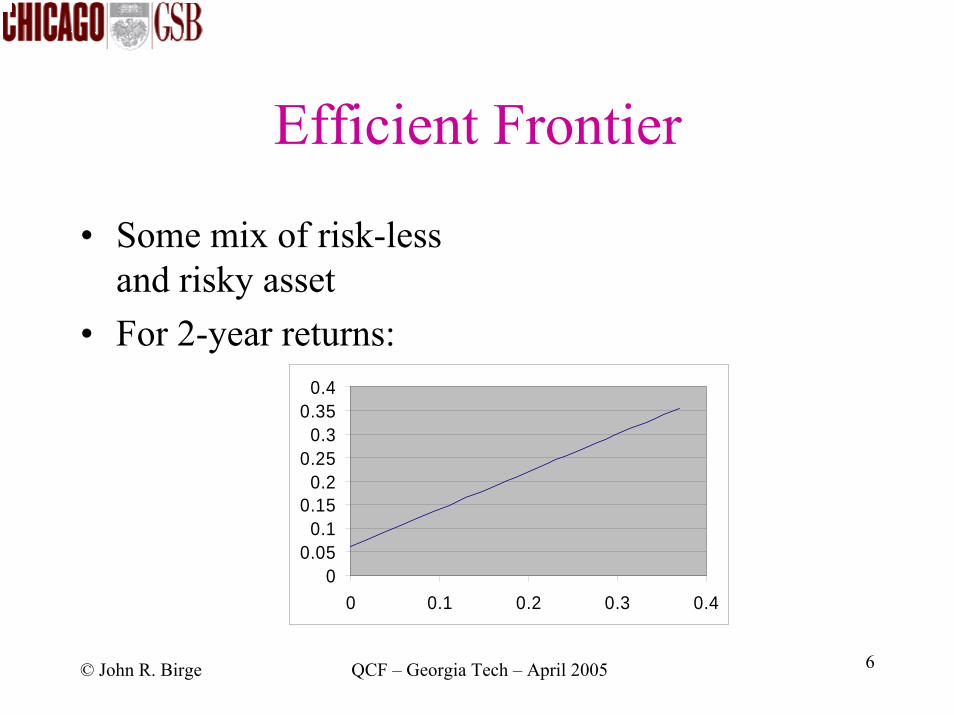
Efficient Frontier

• Some mix of risk-less and risky asset

• For 2-year returns:

00.05

0.10.15

0.20.25

0.30.35

0.4

0 0.1 0.2 0.3 0.4


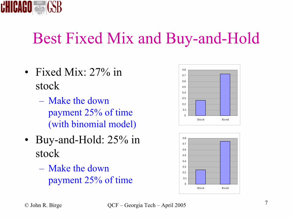
Best Fixed Mix and Buy-and-Hold

• Fixed Mix: 27% in stock– Make the down

payment 25% of time (with binomial model)

• Buy-and-Hold: 25% in stock– Make the down

payment 25% of time

0

0.1

0.2

0.3

0.4

0.5

0.6

0.7

0.8

Sto ck B o nd

0

0.1

0.2

0.3

0.4

0.5

0.6

0.7

0.8

Sto ck B o nd


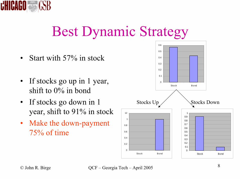
Best Dynamic Strategy

• Start with 57% in stock

• If stocks go up in 1 year, shift to 0% in bond

• If stocks go down in 1 year, shift to 91% in stock

• Make the down-payment 75% of time

0

0.1

0.2

0.3

0.4

0.5

0.6

Sto ck B o nd

0

0.2

0.4

0.6

0.8

1

1.2

Sto ck B o nd0

0.10.20.30.40.50.60.70.80.9

1

Stock Bond

Stocks Up Stocks Down


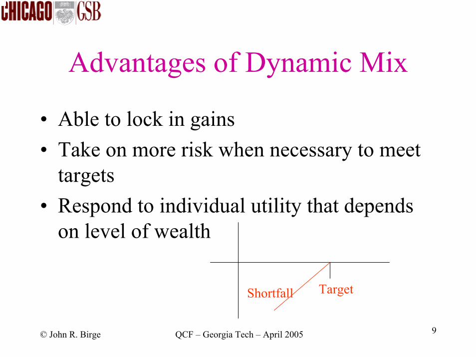
Advantages of Dynamic Mix

• Able to lock in gains• Take on more risk when necessary to meet

targets• Respond to individual utility that depends

on level of wealth

TargetShortfall


Approaches for Dynamic Portfolios• Static extensions

– Can re-solve (but hard to maintain consistent objective)– Solutions can vary greatly– Transaction costs difficult to include

• Dynamic programming policies– Approximation– Restricted policies (optimal – feasible?) – Portfolio replication (duration match)

• General methods (stochastic programs)– Can include wide variety– Computational (and modeling) challenges


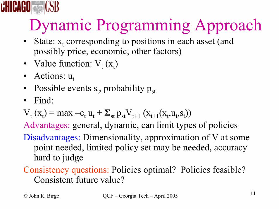
Dynamic Programming Approach• State: xt corresponding to positions in each asset (and

possibly price, economic, other factors)• Value function: Vt (xt)• Actions: ut• Possible events st, probability pst• Find: Vt (xt) = max –ct ut + Σst pstVt+1 (xt+1(xt,ut,st))Advantages: general, dynamic, can limit types of policiesDisadvantages: Dimensionality, approximation of V at some

point needed, limited policy set may be needed, accuracy hard to judge

Consistency questions: Policies optimal? Policies feasible? Consistent future value?


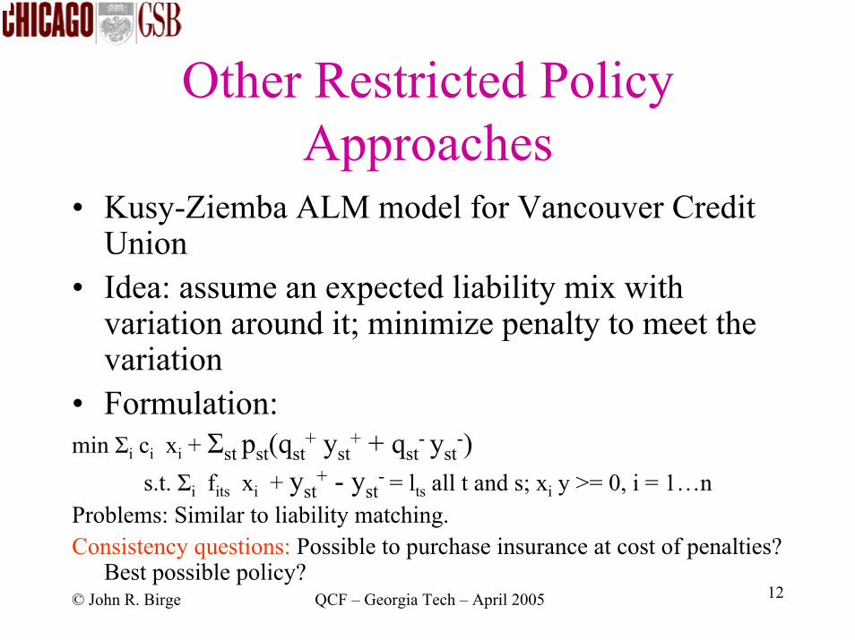
Other Restricted Policy Approaches

• Kusy-Ziemba ALM model for Vancouver Credit Union

• Idea: assume an expected liability mix with variation around it; minimize penalty to meet the variation

• Formulation: min Σi ci xi + Σst pst(qst

+ yst+ + qst

- yst-)

s.t. Σi fits xi + yst+ - yst

- = lts all t and s; xi y >= 0, i = 1…nProblems: Similar to liability matching. Consistency questions: Possible to purchase insurance at cost of penalties?

Best possible policy?


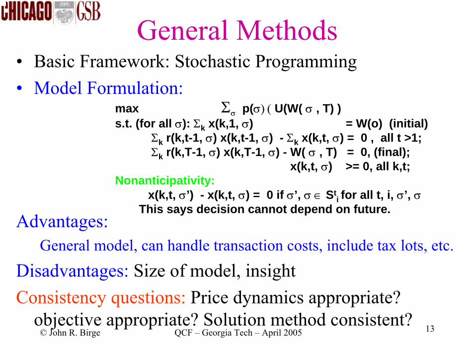
General Methods• Basic Framework: Stochastic Programming • Model Formulation:

Advantages:General model, can handle transaction costs, include tax lots, etc.

Disadvantages: Size of model, insightConsistency questions: Price dynamics appropriate?

objective appropriate? Solution method consistent?

max Σσ p(σ) ( U(W( σ , T) )s.t. (for all σ): Σk x(k,1, σ) = W(o) (initial)

Σk r(k,t-1, σ) x(k,t-1, σ) - Σk x(k,t, σ) = 0 , all t >1;Σk r(k,T-1, σ) x(k,T-1, σ) - W( σ , T) = 0, (final);

x(k,t, σ) >= 0, all k,t;Nonanticipativity:

x(k,t, σ’) - x(k,t, σ) = 0 if σ’, σ ∈ Sti for all t, i, σ’, σ

This says decision cannot depend on future.


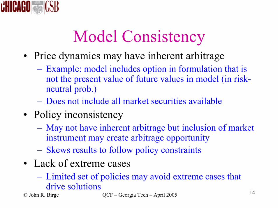
Model Consistency• Price dynamics may have inherent arbitrage

– Example: model includes option in formulation that is not the present value of future values in model (in risk-neutral prob.)

– Does not include all market securities available• Policy inconsistency

– May not have inherent arbitrage but inclusion of market instrument may create arbitrage opportunity

– Skews results to follow policy constraints• Lack of extreme cases

– Limited set of policies may avoid extreme cases that drive solutions


Objective Consistency

• Examples with incoherent objectives– Mean and variance – Probability of beating benchmark

• Coherent measures of risk (Heath et al.)– Can lead to piecewise linear utility function

forms– Expected shortfall, downside risk, or

conditional value-at-risk (Uryasiev and Rockafellar)


Model and Method Difficulties

• Model Difficulties– Arbitrage in tree– Loss of extreme cases– Inconsistent utilities

• Method Difficulties– Deterministic incapable on large problems– Stochastic methods have bias difficulties

• Particularly for decomposition methods• Discrete time approximations

– Stopping rules and time hard to judge


Resolving Inconsistencies

• Objective: Coherent measures • Model resolutions

– Construction of no-arbitrage trees (Klaassen)– Extreme cases (Generalized moment problems

and fitting with existing price observations)• Method resolutions

– Use structure for consistent bound estimates– Decompose for efficient solution


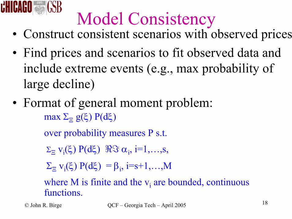
Model Consistency• Construct consistent scenarios with observed prices• Find prices and scenarios to fit observed data and

include extreme events (e.g., max probability of large decline)

• Format of general moment problem:max ΣΞ g(ξ) P(dξ)

over probability measures P s.t.

ΣΞ vi(ξ) P(dξ) <= αi, i=1,…,s,

ΣΞ vi(ξ) P(dξ) = βi, i=s+1,…,M

where M is finite and the vi are bounded, continuous functions.


Extremal Probabilities• Problem: find maximum (risk-neutral equivalent)

probability of price above 55 given observed call premia C:Max ∑j|Sj≥>=55 pjs.t. ∑j pj = 1

∑j pj (Sj-Ki)+ = FV(C(Ki,T))∑j pj Sj = FV(St), pj ≥ 0

For example, suppose Sj = 30, 35,40,45,50,55,60 and Call values: C(35)=10.3, C(40)=5.5, C(45)=2, C(50)=0.5

Result:Prob(ST≥ 55)=0.10

Extend to find sets of probabilities and ranges


Method Consistency: Abridged Nested Decomposition

• Incorporates sampling into the general framework of nested decomposition for stochastic programs

• View as approximate dynamic programming• Samples both the subproblems to solve and the

solutions to continue from in the forward pass of nested decomposition

• Eliminates inconsistency by use of deterministic lower bound and re-sampled upper bound (consistent check of optimality on each iteration)


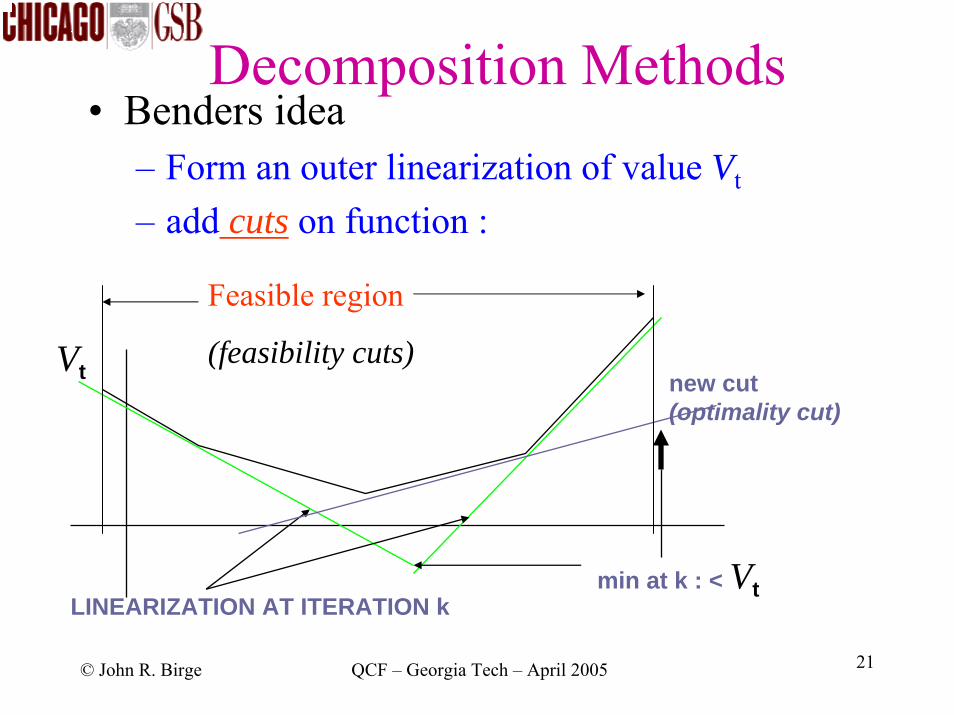
Decomposition Methods• Benders idea

– Form an outer linearization of value Vt

– add cuts on function :

Vt

LINEARIZATION AT ITERATION kmin at k : < Vt

new cut (optimality cut)

Feasible region

(feasibility cuts)


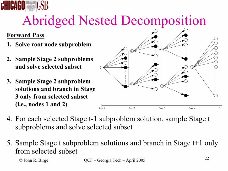
Abridged Nested Decomposition

4. For each selected Stage t-1 subproblem solution, sample Stage t subproblems and solve selected subset

5. Sample Stage t subproblem solutions and branch in Stage t+1 only from selected subset

1

2

3

4

5

Stage 1 Stage 2 Stage 3 Stage 4 Stage 5

Forward Pass1. Solve root node subproblem

2. Sample Stage 2 subproblemsand solve selected subset

3. Sample Stage 2 subproblemsolutions and branch in Stage 3 only from selected subset (i.e., nodes 1 and 2)


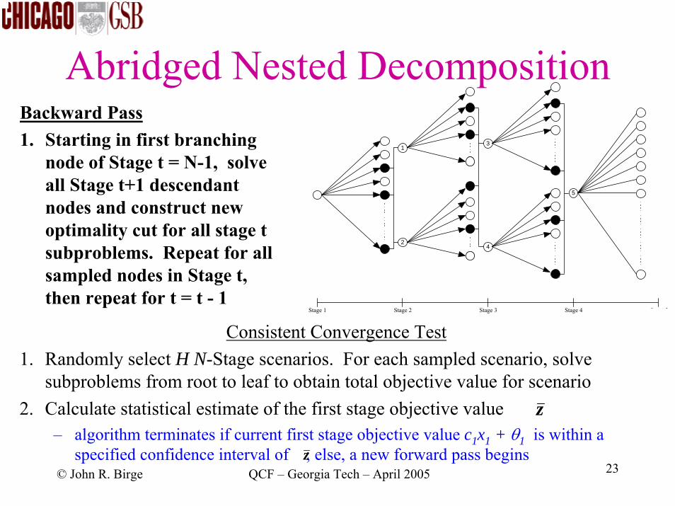
Abridged Nested Decomposition

Consistent Convergence Test1. Randomly select H N-Stage scenarios. For each sampled scenario, solve

subproblems from root to leaf to obtain total objective value for scenario2. Calculate statistical estimate of the first stage objective value

– algorithm terminates if current first stage objective value c1x1 + θ1 is within a specified confidence interval of ; else, a new forward pass begins

1

2

3

4

5

Stage 1 Stage 2 Stage 3 Stage 4 Stage 5

Backward Pass1. Starting in first branching

node of Stage t = N-1, solve all Stage t+1 descendant nodes and construct new optimality cut for all stage t subproblems. Repeat for all sampled nodes in Stage t, then repeat for t = t - 1

z

z


Additional Features for Portfolio Problems

• Serial independence– If increments are serially independent,

formulation is directly applicable• Using structure to relax serial independence

– Can still use structure but assume some serial correlation

– Define a state space determining future price trajectory


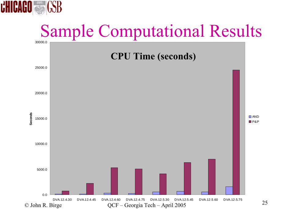
Sample Computational Results

0.0

5000.0

10000.0

15000.0

20000.0

25000.0

30000.0

DVA.12.4.30 DVA.12.4.45 DVA.12.4.60 DVA.12.4.75 DVA.12.5.30 DVA.12.5.45 DVA.12.5.60 DVA.12.5.75

Seco

nds

ANDP&P

CPU Time (seconds)


Summary of Extreme Probability Modeling and AND

• Finding extreme probabilities allows for ranges in sensitivity analysis over distributions and reduced model risk

• Combinations of nested decomposition with outer linearization and sampling allows:– Reduction from exponential to linear effort in number

of re-balance points– Confidence intervals on overall value– Efficient solution relative to alternatives


Challenges

• Extensions for serial correlation• Testing for early termination• Bounds on time-discretization effects• Effective methods for taxable portfolios and

non-convexities (e.g., short-term, long-term)


Conclusions• Dynamic models offer advantages for portfolios

with transaction costs, serial dependence and wealth-dependent objectives

• Stochastic programs provide a general and customizable framework

• Care required in modeling due to arbitrage, coverage of paths, objective consistency and method consistency

• With some effort, models and methods can become consistent

• Efficiency possible with optimization based on structure

Documents

Dynamic Portfolio Optimization with Stochastic Programmingfaculty.chicagobooth.edu/...portfolios_qcf_gatech_1apr2005.pdf · © John R. Birge QCF – Georgia Tech – April 2005 1