DYNAMIC OPTIMIZATION - Essential Microeconomicsessentialmicroeconomics.com/ChapterY6/SlideChapter6.pdf · Essential Microeconomics-1- © John Riley DYNAMIC OPTIMIZATION Life-cycle

Essential Microeconomics -1-

© John Riley

DYNAMIC OPTIMIZATION

Life-cycle consumption and wealth 2

Life-cycle budget constraint 4

Total Wealth accumulation 7

Numerical solution 12

Long finite horizon 13

The infinite horizon problem 14

Family of Dynamic Optimization Problems 17

Malinvaud Condition 18

The Ramsey Problem 24


© John Riley

6.1 LIFE CYCLE CONSUMPTION AND WEALTH

Basic model

A consumer has T periods to live. A single consumption good. Consumption sequence 1{ }Tt tx = .

Our first key simplification is the assumption that preferences can be expressed as an additively

separable concave utility function

11

1( ,..., ) ( ) where ( ) ( )

Tt

T t t t t tt

U x x u x u x u xδ −

=

= =∑ , ( ) 0 and ( ) 0u u′ ′′⋅ > ⋅ < .

We assume that δ lies in the interval [0,1], reflecting the observation that consumers are typically

more focused on immediate concerns than on those in the distant future. Unless otherwise noted, it is

assumed that (0)u′ = ∞ , thereby ensuring that consumption in all periods is strictly positive.

Key assumption

1/11

1

1

( ) 1( , ) ( ) , 0( )

t t tt t

t t

t

Ux u x xMRS x x U u x x

x

σ σδ δ

++

+

+

∂′∂

≡ = = >∂ ′∂

. (6.1-1)

Note that 1( , )t tMRS x x + is independent of the rest of the consumption sequence.


© John Riley

Special case CES preferences

1/11

1

1

( ) 1( , ) ( ) , 0( )

t t tt t

t t

t

Ux u x xMRS x x U u x x

x

σ σδ δ

++

+

+

∂′∂

≡ = = >∂ ′∂

The higher the elasticity of substitution σ , the more slowly the marginal rate of substitution changes as

the consumption ratio increases. The individual is therefore more willing to substitute consumption

between any two periods.

Income sequence 1{ }Tt ty =

Interest rate r

Initial capital 1k

Objective solve for the consumption and capital sequences 1{ }Tt tx = , 1{ }T

t tk = .

Financial Capital accumulation constraint

:tCA 1 (1 )( )t t t tk r k y x+ ≤ + + − . (6.1-2)

Period t+1 capital ≤ (1+r)*(period t capital+ income – consumption)


© John Riley

For period 1 we can rewrite this as follows: 21 1 11

k x y kr≤ + −

+.

Similarly, for period 2, 3 2 2 22(1 ) 1 1 1

k k y xr r r r

≤ + −+ + + +

,

and for period t, 11 1 1(1 ) (1 ) (1 ) (1 )

t t t tt t t t

k k y xr r r r+

− − −≤ + −+ + + +

.

Summing these inequalities and noting that the terms in 2 ,..., Tk k all cancel each other out, we have

11 1 1

1 1(1 ) (1 ) (1 )

T Tt tT

T t tt t

y xk kr r r+

− −= =

≤ + −+ + +∑ ∑ .

In the absence of a bequest motive the consumer will not wish to leave any capital. Moreover no

lender will knowingly allow him to die in debt, therefore 1 0Tk + = . We can therefore rewrite the life-

cycle budget constraint as

11 11 1(1 ) (1 )

T Tt t

t tt t

x ykr r− −

= =

≤ ++ +∑ ∑ .

1{ } { }t tPV x k PV y≤ +


© John Riley

We now write the optimization problem in standard form:

11 1{ } 1 1

{ ( ) | ({ }) 0}(1 )t

T Tt t

t t tx t t

xMax u x k PV yr

δ −−

= =

+ − ≥+∑ ∑ .

Because the maximand is concave and the constraint is linear, the Kuhn-Tucker conditions are both

necessary and sufficient. We form the Lagrangian

11 1

1 1

( ) ( ({ }) )(1 )

T Tt t

t t tt t

xu x k PV yr

δ μ−−

= =

= + + −+∑ ∑L ,

and obtain the Kuhn-Tucker conditions,

11( ) 0

(1 )t

t tt

u xx r

μδ −−

∂ ′= − =∂ +L and 1

1

( ) 0(1 )

tt t

t

u xx r

μδ ++

∂ ′= − =∂ +L .

Eliminating the shadow price from these two equations yields the following necessary condition for a

maximum:

FOC: 1

( ) (1 )( )

t

t

u x ru x

δ+

′= +

′. (6.1-3)


© John Riley

Consider { }tx and { }tx where 1{ }Tt tx = is optimal.

Suppose , , 1s sx x s t t= ≠ +

the present value of the two consumption streams

must be equal

1 1

1 1t t

t tx xx x

r r+ ++ = ++ +

.

This is depicted in Figure 6.1-1.

At the optimum 1( , )t tx x + the steepness of the constraint

must equal the marginal rate of substitution.

Appealing to (6.1-1)

11

( )1( , ) 1( )

tt t

t

u xMRS x x ru xδ+

+

′≡ = +

′.

steepness = 1+r

Figure 6.1-1: Necessary condition


© John Riley

Total Wealth

({ } )Tt t t tW k PV yτ τ == +

= current financial capital + PV future income

111 (1 )

Tt

tt

x Wr −

=

=+∑ , (6.1-4)

Growth of total wealth

Note that if a bank were to take all your future income in period t as collateral it would be willing to

lend you

{ }Tt t t s tW k PV y= +

All your spending now comes out of your total capital tW . The rest accumulates interest. Therefore

1 (1 )( )t t tW r W x+ = + − . (6.1-5)

Exercise: Prove this using the definitions of present value for tW and 1tW + and the financial capital

accumulation equation.


© John Riley

Phase Diagram

Subtracting tW from both sides of (6.1-5),

1 (1 )t t t tW W rW r x+ − = − + .

Thus wealth increases if and only if

tx lies below the line 1t t

rx Wr

=+

.

This line is depicted in Figure 6.1-2.

Below this boundary line wealth is increasing

and above it wealth is decreasing.

Assumption: (1 ) 1rδ + > .

Then consumption increases over the life-cycle, as indicated by the vertical arrows. This figure is

known as a phase diagram because the wealth-consumption dynamics can be separated into two

phases.

Terminal line

Figure 6.1-2: Consumption-Wealth Phase Diagram with

II


© John Riley

If there is no bequest motive, the individual maximizes by leaving no wealth in period 1T + . More

generally, we can allow for a bequest motive by seeking the optimal consumption path that leaves a

period 1T + wealth of 1TW + . Then, in period T, consumption must satisfy 1 (1 )( )T T TW r W x+ = + − .

Rearranging this expression, ( , )T Tx W must lie on the “terminal line”

1

1T

T TWx W

r+= −

+

This last period constraint is depicted in the

figure as the heavy dashed line.

Terminal line

Figure 6.1-2: Consumption-Wealth Phase Diagram with

II


© John Riley

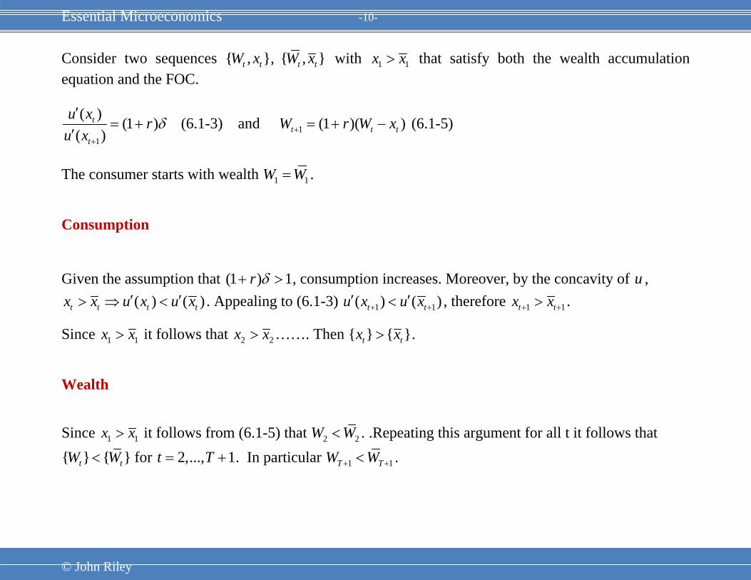
Consider two sequences { , }, { , }t t t tW x W x with 1 1x x> that satisfy both the wealth accumulation equation and the FOC.

1

( ) (1 )( )

t

t

u x ru x

δ+

′= +

′ (6.1-3) and 1 (1 )( )t t tW r W x+ = + − (6.1-5)

The consumer starts with wealth 1 1W W= .

Consumption

Given the assumption that (1 ) 1r δ+ > , consumption increases. Moreover, by the concavity of u , ( ) ( )t t t tx x u x u x′ ′> ⇒ < . Appealing to (6.1-3) 1 1( ) ( )t tu x u x+ +′ ′< , therefore 1 1t tx x+ +> .

Since 1 1x x> it follows that 2 2x x> ……. Then { } { }t tx x> .

Wealth

Since 1 1x x> it follows from (6.1-5) that 2 2W W< . .Repeating this argument for all t it follows that { } { }t tW W< for 2,..., 1t T= + . In particular 1 1T TW W+ +< .


© John Riley

Numerical solution

For any initial wealth 1W and choice 1x , there is a unique sequence of consumption 1{ }Tt tx = and wealth

12{ }T

t tW += satisfying the FOC and wealth accumulation equation. We have also seen that the mapping

1 1: Tg x W +→ is strictly decreasing. Thus for any bequest 1TW + there is a unique *1x which also satisfies

the terminal constraint 1 1T TW W+ +=

Example:

( ) ln( )t tu x xξ= +

FOC: 11

( )( , ) 1( )

tt t

t

xMRS x x rx

ξδ ξ

++

+= = +

+ . Then 1 (1 ) ( )t tx r xδ ξ ξ+ = + + −

Wealth equation: 1 (1 )( )t t tW r W x+ = + −

The consumption and wealth sequences are depicted below.*

*The spreadsheet can be downloaded from the web-page.

Essential Mic

© John Riley

croeconomiccs -12-


© John Riley

Life-cycle as the time horizon grows large

We consider CES preferences 1/1

1

( ) ( )( )

t t

t t

u x xu x x

σ+

+

′=

′. Substituting this into the FOC and rearranging,

1 ( (1 )) (1 )t

t

x r rx

σδ α+ = + = + where 1((1 ) )r σα δ δ −= + . (6.1-6)

Assumption 1: (1 ) 1rδ + > { }tx is increasing.)

Assumption 2: 1α < Consumption growth rate is les then the interest rate.)

Note that ln ln ( 1)ln((1 ) )rα δ σ δ= + − + . Thus as σ increases, so does lnα and hence α . Moreover,

if 1σ = , then 1α δ= < . Therefore 1α < for all 1σ ≤ . However, because (1 ) 1r δ+ > , α exceeds 1 for

sufficiently large σ .

Life cycle budget constraint

21 1 11({ }) ... ({ })

1 (1 )T

t tT

x xPV x x k PV y Wr r −= + + + = + =

+ +

But 1 1(1 ) (1 )t tt tx r x r xα α+ = + = + . Therefore

1 11 1 1 1 1({ }) ... (1 ... )T T

tPV x x x x x Wα α α α− −= + + + = + + + =


© John Riley

Therefore 1 11( )1

T

x Wαα

−=

−.

By the same argument, optimization from t yields 11( )

1

T t

t tx Wαα

− +−=

−.

Rearranging, 1

1

11 T

xW

αα−

=−

, 21

2

11 T

xW

αα −

−=

−, …, 1

11

tT t

t

xW

αα − +

−=

−

Thus, holding t constant, the longer the time horizon, the larger the denominator. Therefore the ratio

/t tx W decreases with longer T. For short horizons the starting point is above the phase boundary and

so wealth is decreasing in each period. For long horizons the time path goes through two phases. In

phase I wealth rises. Then in phase II wealth declines until the terminal line is reached.

Note finally that if T is very large relative to t,

1t

t

xW

α≈ −


© John Riley

Important Observation

There is a class of problems (such as this one) for which the impact of the time horizon on optimal

choices in the early periods diminishes to zero as the time horizon grows long. Thus, for long finite

horizons, we can approximate the optimal path by taking the limit and letting the horizon approach

infinity.

In such cases it is tempting to conjecture that the limiting sequence { , }t tx W satisfying

(1 )t tx Wα= −

is the solution to the infinite horizon optimization problem

11{ , } 1

{ ( ) | (1 )( )}t t

tt t t tx W t

Max u x W r W xδ∞

−+

=

= + −∑ .

Infinite Horizon Problems with No Solution

Assumption 2′: 1α >

1 1 11 1( ) ( )1 1

T T

x x Wα αα α

− −= =

− − Then 1 1

1( )1Tx Wα

α−

=−


© John Riley

Note that the denominator increases without bound as T →∞ . Therefore for any t, 0tx → as T →∞ .

Thus the limit of the finite horizon solution is for the consumer to delay consumption indefinitely!

Clearly this is not optimal because the consumer would be strictly better off consuming all his or her

wealth in the first period.

This argument suggests strongly that there is no solution to the infinite horizon problem. Although we

will not provide a formal argument, this intuition is correct. To strengthen the intuition, suppose that

preferences are linear so that the T period optimization problem is

11{ , } 1

{ | (1 )( )}t t

tt t t tx W t

Max x W r W xδ∞

−+

=

= + −∑

As long as (1 ) 1r δ+ > , it is easily checked that it is optimal to defer all consumption until period T.

Because there is no last period in the infinite horizon problem, there is no optimal solution.


© John Riley

6.2 A FAMILY OF DYNAMIC OPTIMIZATION PROBLEMS

1 1

11 1 1 1

{ , } 1{ ( , ), | ( , ), ( , ) 0, 1,..., and }

Tt t t

Tt

t t t t t t t t T Tx k tMax u x k k g x k x k t T k kδ

+ =

−+ + + +

=

≤ ≥ = =∑

The initial capital stock is 1k .

For many applications there is no natural terminal date so it is natural to seek a solution to the infinite

horizon optimization problem

1 1

1 1{ , } 1

{ ( , ), | ( , ), ( , ) 0, }t t t

t t t t t t t t tc k tMax u x k k g x k c k t

∞+ =

∞

+ +=

≤ ≥ ∀∑

Suppose that 1{ , }t t tc k ∞= solves this problem. Fix 1 1T Tk k+ += . Then 1{ , }T

t t tc k = must solve

1 1 1{ , } 1{ ( , ) | ( , ), }

t t

T

t t t t t t T Tc k tMax u c k k g c k k k+ + +

=

≤ =∑ .

Thus the FOC for the finite horizon problem must hold for all t T≤ . Because this is true for all T it

follows that the FOC for a finite time horizon must hold for all t in the infinite horizon problem.


© John Riley

For any 1c the FOC and growth equation map out a sequence 1{ , }t t tc k ∞= . Suppose that there is a

sequence 1{ , }t t tc k ∞= satisfying the FOC, the capital accumulation constraints and the non-negativity

constraints for all t. We show that if the problem is concave and the shadow value of the capital stock

1t tkλ + , has a limiting value of zero, then this path is indeed an optimal path.

Proposition 6.2-1: Malinvaud Condition1

Suppose that ( )tu ⋅ and ( ), 1,...tg t⋅ = are concave functions and 1{ , }t t tc k ∞= satisfies the Kuhn-

Tucker conditions and feasibility constraints. If the value of the capital stock approaches zero, that is

1{ } 0t tkλ + → , then for any other feasible sequence 1{ , }t t tc k ∞= and any 0ε > there exists a T̂ such that for

all ˆT T>

1 1

( , ) ( , )T T

t t t t t tt t

u c k u c k ε= =

≤ +∑ ∑ .

Note that the sums on both sides may not converge to a limit at T gets large.

1 This condition is also known as the transversality condition.


© John Riley

Proof: Define 1 2 1( , ) ( ,..., , ,.., )T Tx k x x k k += and let ( , )x k be the solution to the finite horizon

optimization problem with final capital 1Tk + . Then we need to compare the sequences 1( , )Tx k + and

1( , )Tx k + .

The Lagrangian for the optimization problem is

11 1

( , , ) ( , ) ( ( , ) )T T

t t t t t t t tt t

x k u x k g x k kλ λ += =

= + −∑ ∑L .

Because ( , , )x k λL is a concave function of ( , )x k ,

( , , ) ( , , )x k x kλ λ≤L L .

( , , ) ( ) ( , , )( )x k x x x k k kx k

λ λ∂ ∂+ ⋅ − + −∂ ∂L L (6.2-1)

From the FOC

( , , ) 0, 1,...,t

x k t Tx

λ∂≤ =

∂L and ( , , ) 0, 2,...,

t

x k t Tk

λ∂≤ =

∂L .

Also


© John Riley

1

( , , ) 0TT

x kk

λ λ+

∂= − ≤

∂L .

For feasibility ( , ) 0x k ≥ . Therefore

( , , ) 0x k xx

λ∂⋅ ≤

∂L and ( , , ) 0x k k

kλ∂⋅ ≤

∂L .

Substituting into (S.2-1)

( , , ) ( , , )x k x kλ λ≤L L ( , , ) ) ( , , )x k x x k kx k

λ λ∂ ∂− ⋅ − ⋅∂ ∂L L

By complementary slackness,

( , , ) 0, 1,...,tt

x x k t Tx

λ∂= =

∂L and ( , , ) 0, 2,...,t

t

k x k t Tk

λ∂= =

∂L .

Therefore

11

( , , ) ( , , ) ( , , ) TT

x k x k x k kk

λ λ λ ++

∂≤ −

∂L

L L = 1( , , ) T Tx k kλ λ ++L

That is

1 1 11 1 1 1

( , ) ( ( , ) ) ( , ) ( ( , ) )T T T T

t t t t t t t t t t t t t t t t T Tt t t t

u x k g x k k u x k g x k k kλ λ λ+ + += = = =

+ − ≤ + − +∑ ∑ ∑ ∑


© John Riley

From the Kuhn-Tucker conditions the second sum on the right-hand side is zero. For feasibility,

1( , ) 0t t t tg x k k +− ≥ so the second sum on the left-hand side is positive. Therefore

11 1

( , ) ( , )T T

t t t t t t T Tt t

u x k u x k kλ += =

≤ +∑ ∑ .

If the value of the capital stock has a limit of zero it follows that for any ε there exists a T̂ such that

for all ˆT T>

1 1( , ) ( , )

T T

t t t t t tt t

u x k u x k ε= =

≤ +∑ ∑ .

Q.E.D.


© John Riley

An Example: Optimal Wealth Accumulation with CES preferences

As an illustration, consider the finite horizon wealth accumulation problem

1

11 1 1

{ , ) 1{ ( ) | (1 )( ), }

Tt t t

Tt

t t t T Tx W tMax u x W r W x W Wδ

=

−+ + +

=

≤ + − ≥∑

and its infinite horizon counterpart

1

11

{ , ) 1{ ( ) | (1 )( )}

t t t

tt t t

x W tMax u x W r W xδ

∞=

∞−

+=

≤ + −∑ .

The Lagrangian for the finite horizon problem is

11 1 1

1 1( ) ((1 )( ) ) ( )

T Tt

t t t t t T Tt t

u x r W x W W Wδ λ μ−+ + +

= =

= + + − − + −∑ ∑L .

For any 1 0tW + > , 11

(1 ) 0t tt

rW

λ λ++

∂= + − =

∂L .

Thus

1 11

t

t rλλ+ =

+ .


© John Riley

Consumption growth

As we have seen, the FOC is

1 (1 )t tx r xα+ = +

Consider the sequence { , } {(1 ) , }t t t tx W W Wα= − .

Capital accumulation

1 (1 )( ) (1 )( (1 ) ) (1 )t t t t t tW r W x r W W r Wα α+ = + − = + − − = +

Thus consumption and capital grow at the same constant rate.

Note also that

11 1 1 11 ((1 ) ) (1 )

(1 )t t

t t tW r W r Wrλλ α λ α+ −= + = ++

.

The right hand side approaches zero in the limit if 1α < .

and so the Malinvaud Condition is satisfied.


© John Riley

6.3 THE RAMSEY PROBLEM

Representative agent economy

1

1( )t

tt

U u xδ∞

−

=

=∑ .

Assumption 1: ( )u ⋅ is strictly concave and (0)u′ = ∞ .

At time t the capital stock is tk . This yields an output of ( )tq k , where ( )q ⋅ is a strictly increasing and

strictly concave function. The consumer must decide how much of this output to invest and how

much to consume. Let ti be period t investment. Then

( )t t tx i q k+ = .

Capital depreciates at a rate θ . Thus with gross investment ti , the capital stock next period is

1 (1 ) (1 ) ( )t t t t t tk k i k q k xθ θ+ = − + = − + − .

We write this more simply as

1 ( )t t tk F k x+ = − where ( ) (1 ) ( )t t tF k k q kθ= − + . (19.3-1)

Because we have assumed that the gross output function ( )q ⋅ is strictly concave, the net output

function ( )F ⋅ is also strictly concave. For simplicity we also assume that ( )F ⋅ is strictly increasing.


© John Riley

To solve the representative agent’s optimization problem, we begin by using the Lagrange method to

obtain necessary conditions for the finite horizon version of the problem

11

1( ) ( ( ) )

Tt

t t t t tt

u x F k k xδ λ−+

=

= + − −∑L .

Ignoring the possibility of a boundary solution, the first-order conditions are

1 ( ) 0tt t

t

u xx

δ λ−∂ ′= − =∂L , (19.3-2)

and

1( ) 0t t tt

F kk

λ λ −

∂ ′= − =∂L . (19.3-3)

Combining these conditions yields the necessary condition

11

( )( , ) ( )( )t

t t tt

u xMRS x x F ku xδ

−−

′′= =

′, 2,...t = (19.3-4)

To draw the phase diagram we first note that, from (19.3-4), 1( ) ( ) ( )t t tu x F k u xδ−′ ′ ′= . Thus

1( ) ( )t tu x u x−′ ′> if and only if ( ) 1tF kδ ′ > . Because ( )u ⋅ is strictly concave, it follows that

1t tx x −> if and only if ( ) 1tF kδ ′ > .


© John Riley

Suppose that for some capital stock Sk ,

( ) 1SF kδ ′ = . Because ( )F ⋅ is strictly concave

there can be at most one such capital stock.

Then consumption is increasing if and only if

t Sk k< . The vertical consumption arrows are

therefore as depicted in the phase diagram

in Figure 6.3-1.

Next consider capital accumulation.

The accumulation constraint (19.3-1) can be

rewritten as follows:

1 ( ) .t t t t tk k F k x k+ − = − −

Thus capital is increasing if and only if ( , )t tx k lies below the phase boundary

( )t t tx F k k= − .

The phase diagram is then as depicted in Figure 6.3-1. Consumption increases if and only if the

economy is in phases II or III. Capital grows if and only if the economy is in phases III or IV.

I

Figure 6.3-1: Phase Diagram

A

S


© John Riley

Starting from a low capital stock, there is a sequence 1{ , }t t tx k ∞= in phase III that approaches the

stationary point S. This is depicted in the figure as the curve AS. Note that, because the consumption

path approaches Sx , it follows directly from (19.3-2) that the sequence of shadow prices approaches

zero. Also the limiting capital stock is finite. Thus the value of the capital stock 1t tkλ + approaches

zero so the Malinvaud Condition holds. Given the concavity of the production function and utility

function, it follows that the sequence 1{ , }t t tx k ∞= is optimal.

Documents

DYNAMIC OPTIMIZATION - Essential Microeconomicsessentialmicroeconomics.com/ChapterY6/SlideChapter6.pdf · Essential Microeconomics-1- © John Riley DYNAMIC OPTIMIZATION Life-cycle