Dynamic Optimization Dr. Abebe Geletu Ilmenau University of Technology Department of Simulation and Optimal Processes (SOP)

sop

Dynamic Optimization

Dr. Abebe Geletu

Ilmenau University of TechnologyDepartment of Simulation and Optimal Processes

(SOP)

www.tu-ilmenau.de/simulationSeite 1

sop

Chapter 1: Introduction

www.tu-ilmenau.de/simulationSeite 2

"A system is a self-contained entity with interconnected elements, process and parts. A system can be the design of nature ora human invention."

A system is an aggregation of interactive elements.

• A system has a clearly defined boundary. Outside this boundary is the environment surrounding the system.• The interaction of the system with its environment is the most vital aspect. • A system responds, changes its behavior, etc. as a result of influences (impulses) from the environment.

1.1 What is a system?

sop Seite 3 www.tu-ilmenau.de/simulation

Course ContentChapters1. Introduction2. Mathematical Preliminaries3. Numerical Methods of Differential Equations4. Modern Methods of Nonlinear Constrained Optimization Problems5. Direct Methods for Dynamic Optimization Problems6. Introduction of Model Predictive Control (Optional)

References:

sop www.tu-ilmenau.de/simulationSeite 4

1.2. Some examples of systems

• Water reservoir and distribution network systems• Thermal energy generation and distribution systems • Solar and/or wind-energy generation and distribution systems• Transportation network systems• Communication network systems• Chemical processing systems• Mechanical systems• Electrical systems• Social Systems• Ecological and environmental system• Biological system• Financial system• Planning and budget management system• etc


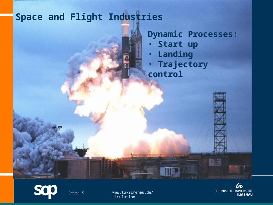
Space and Flight Industries

Dynamic Processes:• Start up• Landing• Trajectory control


Chemical Industries Dynamic Processes:• Start-up• Chemical reactions• Change of Products • Feed variations• Shutdown


Industrial Robot

Dynamische Processes:

• Positionining

• Transportation


1.3. Why System Analysis and Control?

• study how a system behaves under external influences• predict future behavior of a system and make necessary preparations• understand how the components of a system interact among each other• identify important aspects of a system – magnify some while subduing others, etc.

1.3.1 Purpose of systems analysis:


Strategies for Systems Analysis

• System analysis requires system modeling and simulation simulation

• A model is a representation or an idealization of a system.• Modeling usually considers some important aspects and processes of a system.• A model for a system can be:• a graphical or pictorial representation• a verbal description• a mathematical formulationindicating the interaction of components of the system


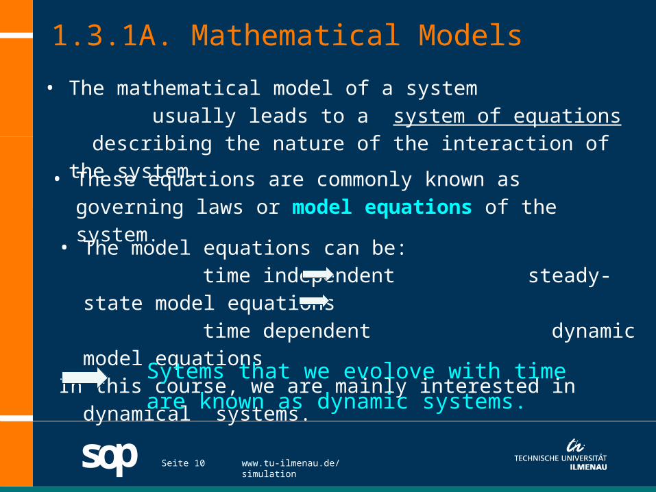
1.3.1A. Mathematical Models

• The mathematical model of a system usually leads to a system of equations describing the nature of the interaction of the system.

• The model equations can be: time independent steady-state model equations time dependent dynamic model equationsIn this course, we are mainly interested in dynamical systems.

• These equations are commonly known as governing laws or model equations of the system.

Sytems that we evolove with time are known as dynamic systems.


• Linear Differential Equations

• Example RLC circuit (Ohm‘s and Kirchhoff‘s Laws)

•

BuAxx

1.3.2. Examples of dynamic models

vuLBC

LLR

Av

iv

i

CC

,0

1 ,

01

1 ,x , x

vLv

i

C

LLR

v

i

CC

0

1

01

1


• Nonlinear Differential equations

)),(),(()( ttutxftx



• Nonlinear Differential equations

)),(),(()( ttutxftx

0)(15)(20

0105)(

220)(155

13233

2232

311

iiiiRi

iiiiR

Viii



1.3.1B Simulation

• studies the response of a system under various external influences – input scenarios

• for model validation and adjustment – may give hint for parameter estimation

• helps identify crucial and influential characterstics (parameters) of a system

• helps investigate: instability, chaotic, bifurcation behaviors in a systems dynamic as caused by certain external influences• helps identify parameters that need to be controlled


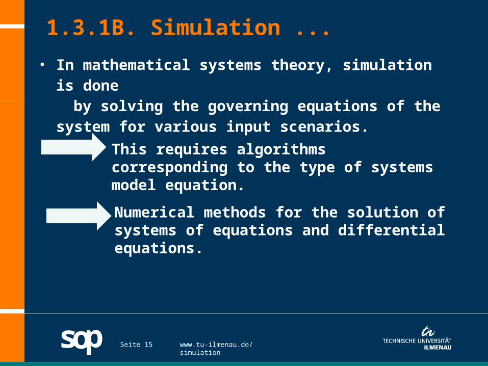
1.3.1B. Simulation ...

• In mathematical systems theory, simulation is done by solving the governing equations of the system for

various input scenarios.

This requires algorithms corresponding to the type of systems model equation.

Numerical methods for the solution of systems of equations and differential equations.


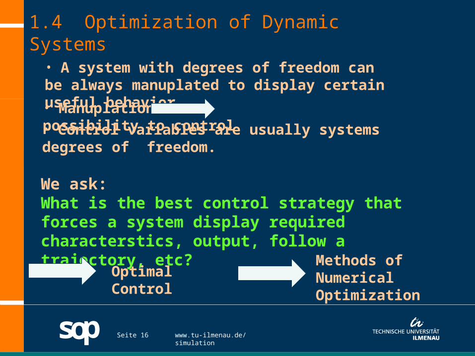
1.4 Optimization of Dynamic Systems

• A system with degrees of freedom can be always manuplated to display certain useful behavior.

• Manuplation possibility to control• Control variables are usually systems degrees of freedom.

We ask: What is the best control strategy that forces a system display required characterstics, output, follow a trajectory, etc?

Optimal ControlMethods of Numerical Optimization


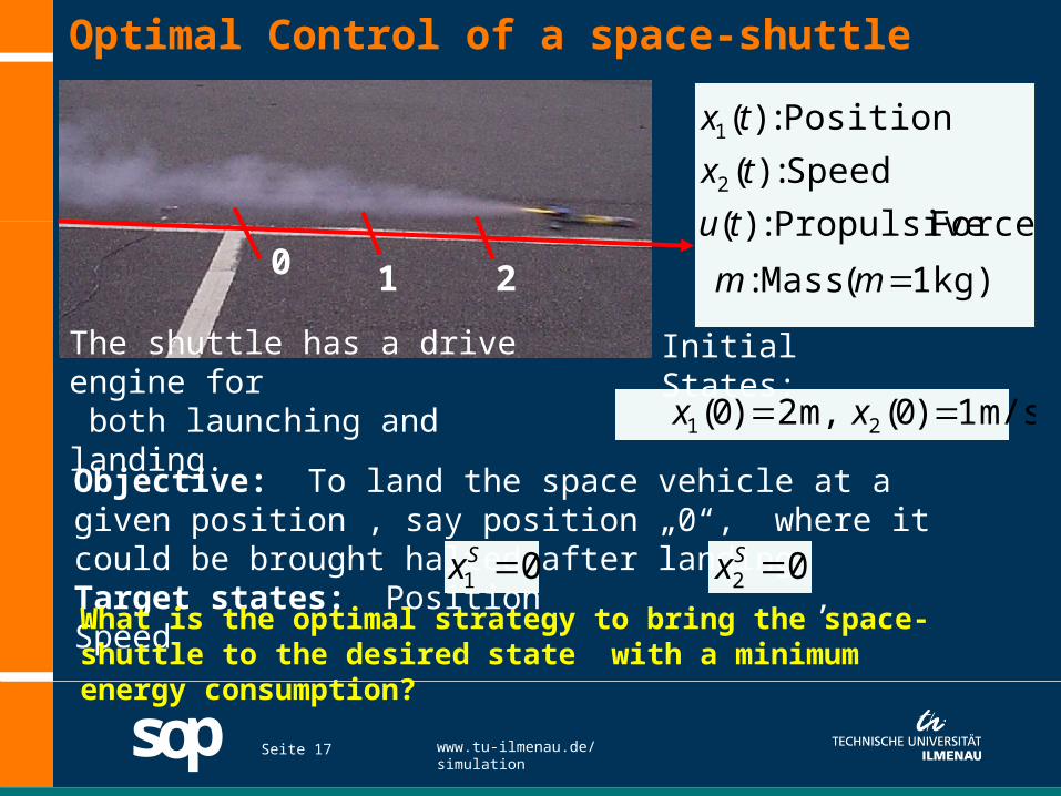
Optimal Control of a space-shuttle

0 1 2

Force Propulsive:)(

Speed:)(

Position:)(

2

1

tu

tx

tx

kg) 1( Mass: mm

Initial States:

m/s1)0( m,2)0( 21 xxThe shuttle has a drive engine for both launching and landing.

Objective: To land the space vehicle at a given position , say position „0“, where it could be brought halted after landing.Target states: Position , Speed01 Sx 02 SxWhat is the optimal strategy to bring the space-shuttle to the desired state with a minimum energy consumption?


Optimal Control of a space-shuttle

0 1 2

Force Propulsive:)(

Speed:)(

Position:)(

2

1

tu

tx

tx

kg) 1( Mass: mm

Model Equations:

)()()(

)()(

2

21

txmtamtu

txtx

Then

)(1

)(

)()(

2

21

tum

tx

txtx

ux

x

x

x

1

0

00

10

2

1

2

1

Hence BuAxx Objectives of the optimal control:

• Minimization of the error: )();( 2211 txxtxx SS •Minimization of energy: )(tu


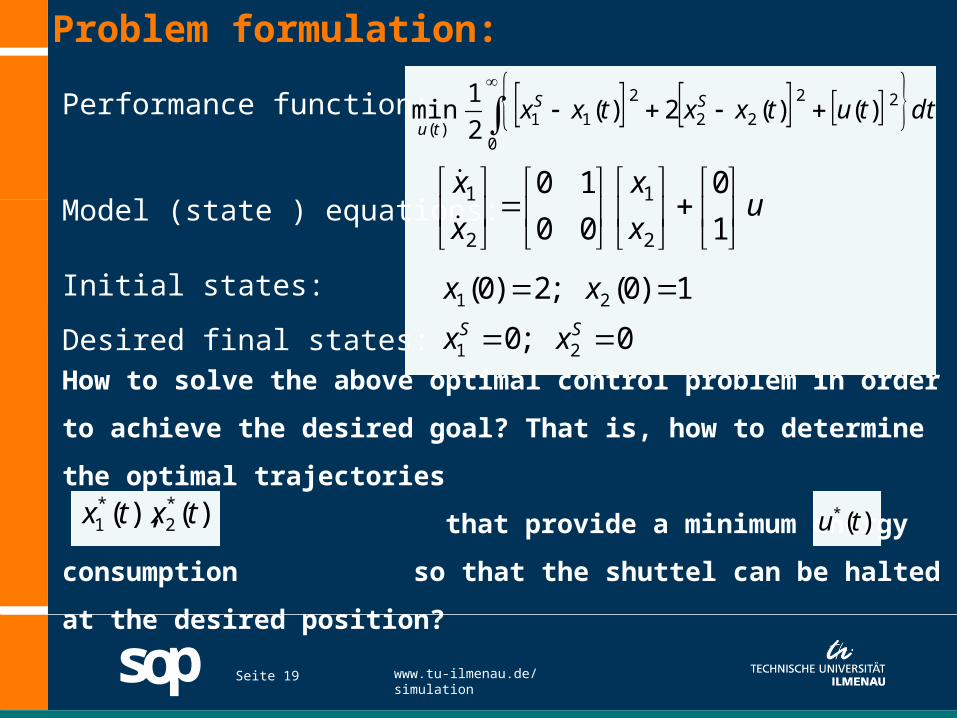
Problem formulation:

Performance function:

0

22

22

2

11)(

)()(2)(2

1min dttutxxtxx SS

tu

Model (state ) equations: ux

x

x

x

1

0

00

10

2

1

2

1

Initial states:

0;0

1)0(;2)0(

21

21

SS xx

xx

Desired final states:

How to solve the above optimal control problem in order to achieve

the desired goal? That is, how to determine the optimal trajectories

that provide a minimum energy consumption so

that the shuttel can be halted at the desired position?

)(),( *2

*1 txtx )(* tu


Optimal Operation of a Batch Reactor


Optimal Operation of a Batch Reactor

Some basic operations of a batch reactor

• feeding Ingredients

• adding chemical catalysts

• Raising temprature

• Reaction startups

• Reactor shutdown

TC

Tsoll

Chemical ractions: CBAorder1st order 2nd

Initial states: 0)0(,0)0(mol/l,1)0( CBA CCC

Objective: What is the optimal temperature strategy, during the operation of the reactor, in order to maximize the concentration of komponent B in the final product?

Allowed limits on the temperature: KTK 398298


Mathematical Formulation: Objective of the optimization: )(max

)(fB

tTtC

BC

BAB

AA

CTkdt

dC

CTkCTkdt

dC

CTkdt

dC

)(

)()(

)(

2

22

1

21

RT

EkTk

RT

EkTk

2202

1101

exp)(

exp)(

KTK 398298

0)0(,0)0(mol/l,1)0( CBA CCC

ftt 0

Model equations:

Process constraints:

Initial states:

Time interval:

This is a nonlinear dynamic optimization problem.


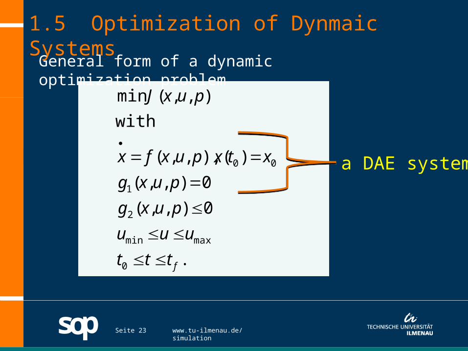
1.5 Optimization of Dynmaic Systems

.

0),,(

0),,(

)(),,,(

with

),,(min

0

maxmin

2

1

00

fttt

uuu

puxg

puxg

xtxpuxfx

puxJ

a DAE system

General form of a dynamic optimization problem


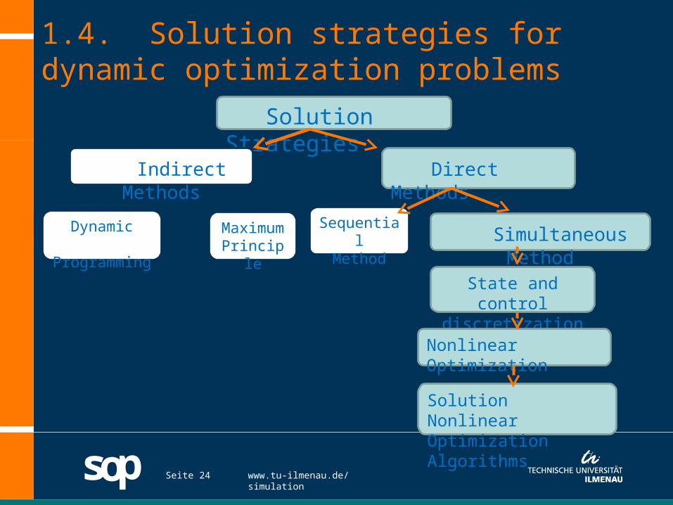
1.4. Solution strategies for dynamic optimization problems

Solution Strategies

Indirect Methods Direct Methods

Dynamic Programming

Maximum Principle

Simultaneous MethodSequential

Method

State and control discretization

Nonlinear Optimization

Solution Nonlinear Optimization Algorithms


Solution strategies for dynamic optimization problems

Indirect methods (classical methods)

• Calculus of variations ( before the 1950‘s)

• Dynamic programming (Bellman, 1953)

• The Maximum-Principle (Pontryagin, 1956)1Lev Pontryagin

Direct (or collocation) Methods (since the 1980‘s)

• Discretization of the dynamic system

• Transformation of the problem into a nonlinear optimization problem

• Solution of the problem using optimization

algorithms Verfahren


Collocation Method

1.5. Nonlinear Optimization formulation of dynamic optimization problem

.

0),,(

0),,(

),,(min

maxmin uUu

pUXG

pUXF

with

pUXEU

• After appropriate renaming of variables we obtain a non-linear programming problem (NLP)

Documents

Dynamic Optimization Dr. Abebe Geletu Ilmenau University of Technology Department of Simulation and Optimal Processes (SOP)