Embed Size (px)
Citation preview

DYNAMIC NONLINEAR BENDING AND
TORSION OF A CANTILEVER BEAM
THESIS
Michael S. Whiting, Captain, USAF
AFIT/GAE/ENY/06-M32
DEPARTMENT OF THE AIR FORCE AIR UNIVERSITY
AIR FORCE INSTITUTE OF TECHNOLOGY
Wright-Patterson Air Force Base, Ohio
APPROVED FOR PUBLIC RELEASE; DISTRIBUTION UNLIMITED

The views expressed in this thesis are those of the author and do not reflect the official policy or position of the United States Air Force, Department of Defense, or the United States Government.

AFIT/GAE/ENY/06-M32
DYNAMIC NONLINEAR BENDING AND TORSION OF A CANTILEVER BEAM
THESIS
Presented to the Faculty
Department of Aeronautics and Astronautics
Graduate School of Engineering and Management
Air Force Institute of Technology
Air University
Air Education and Training Command
In Partial Fulfillment of the Requirements for the
Degree of Master of Science in Aeronautical Engineering
Michael S. Whiting, BS
Captain, USAF
June 2006
APPROVED FOR PUBLIC RELEASE; DISTRIBUTION UNLIMITED.

AFIT/GAE/ENY/06-M32 DYNAMIC NONLINEAR BENDING AND TORSION OF A CANTILEVER BEAM
Michael S. Whiting, BS Captain, USAF
Approved: ____________________________________ Donald L. Kunz (Chairman) date ____________________________________ Robert A. Canfield (Member) date ____________________________________ Richard G. Cobb (Member) date

AFIT/GAE/ENY/06-M32
Abstract
This effort sought to measure the dynamic nonlinear bending and torsion response
of a cantilever beam. The natural frequencies of a cantilever beam in both chord and flap
directions were measured at different static root pitch angles with varying levels of
weights attached at the free end. The results were compared with previous
experimentation to validate the data and testing procedures while lowering the associated
error bands. Additionally, methodology for measuring mode shapes was set forth and
mode shapes were measured for a few test cases with zero degrees of root pitch.
iv

AFIT/GAE/ENY/06-M32
To My Loving Wife
v

Acknowledgments
I would like to express my sincere appreciation to my faculty advisor, Dr. Donald
Kunz, for his guidance and patience throughout the course of this thesis effort.
Michael S. Whiting
vi

Table of Contents
Page
Abstract .............................................................................................................................. iv
Dedication ........................................................................................................................... v
Acknowledgments.............................................................................................................. vi
List of Figures .................................................................................................................... ix
List of Tables ...................................................................................................................... x
List of Symbols .................................................................................................................. xi
I. Introduction................................................................................................................... 1
Princeton Beam Experiment ......................................................................................... 1 Static Tests .............................................................................................................. 1 Dynamic Tests ........................................................................................................ 2 Comparison to Theory ............................................................................................ 2 Follow-on Experimentation .................................................................................... 3 Application.............................................................................................................. 3 Limitations .............................................................................................................. 4
Research Objectives.......................................................................................................4
II. Methodology................................................................................................................. 6
Parts Fabrication ........................................................................................................... 6 Beams...................................................................................................................... 6 Tip Weights............................................................................................................. 6
Set-Up ......................................................................................................................... 10 Accelerometers ..................................................................................................... 11 Laser Vibrometer .................................................................................................. 13
Instrumentation Choices ..............................................................................................15
III. Results and Analysis ................................................................................................... 16
Differences in Methodology ....................................................................................... 16 Error Calculations ....................................................................................................... 17 Natural Frequencies .................................................................................................... 19
vii

Page
Mode Shapes................................................................................................................23
IV. Conclusions and Recommendations ........................................................................... 27
Accelerometer Results ................................................................................................ 27 Laser Vibrometer Results ........................................................................................... 27 Laser Vibrometer Evaluation...................................................................................... 28
Frequency Resolution ........................................................................................... 28 Twist ..................................................................................................................... 29 Static Measurements ............................................................................................. 29 Beam Geometry .................................................................................................... 30 Benefits ................................................................................................................. 30
Future Experimentation ...............................................................................................30
Appendix A. Data ............................................................................................................ 32
Appendix B. Linear Theory ............................................................................................. 45
Bibliography ..................................................................................................................... 47
Vita.................................................................................................................................... 49
viii

List of Figures
Figure Page
1. Weight Cross Sections .................................................................................................. 7
2. Tip Weights................................................................................................................... 8
3. Moment of Inertia Equation Variables ......................................................................... 9
4. Swivel Attachment...................................................................................................... 10
5. Directional Orientation ............................................................................................... 11
6. Accelerometer Locations ............................................................................................ 12
7. Scanning Laser Vibrometer Set-up............................................................................. 14
8. Reduction in Error Bands............................................................................................ 18
9. Flapwise Frequency vs. Pitch Angle........................................................................... 19
10. Chordwise Frequency vs. Pitch Angle........................................................................ 20
11. Flapwise Frequency vs. Tip Load............................................................................... 22
12. Chordwise Frequency vs. Tip Load ............................................................................ 22
13. Flapwise Mode 1......................................................................................................... 24
14. Flapwise Mode 2......................................................................................................... 25
15. Flapwise Mode 3......................................................................................................... 26
ix

List of Tables
Table Page
1. Tip Weight Dimensions ................................................................................................ 8
2. Frequency Limitations ................................................................................................ 29
3. Accelerometer Data .................................................................................................... 32
4. Princeton Beam Data (Included for Reference).......................................................... 34
5. Laser Vibrometer Data, 0 lb Tip Load, 0 degrees Pitch, Mode 1 ............................... 35
6. Laser Vibrometer Data, 0 lb Tip Load, 0 degrees Pitch, Mode 2 ............................... 36
7. Laser Vibrometer Data, 0 lb Tip Load, 0 degrees Pitch, Mode 3 ............................... 37
8. Laser Vibrometer Data, 1 lb Tip Load, 0 degrees Pitch, Mode 1 ............................... 37
9. Laser Vibrometer Data, 1 lb Tip Load, 0 degrees Pitch, Mode 2 ............................... 38
10. Laser Vibrometer Data, 1 lb Tip Load, 0 degrees Pitch, Mode 3 ............................... 39
11. Laser Vibrometer Data, 2 lb Tip Load, 0 degrees Pitch, Mode 1 ............................... 40
12. Laser Vibrometer Data, 2 lb Tip Load, 0 degrees Pitch, Mode 2 ............................... 40
13. Laser Vibrometer Data, 3 lb Tip Load, 0 degrees Pitch, Mode 3 ............................... 41
14. Laser Vibrometer Data, 3 lb Tip Load, 0 degrees Pitch, Mode 1 ............................... 42
15. Laser Vibrometer Data, 3 lb Tip Load, 0 degrees Pitch, Mode 2 ............................... 43
16. Laser Vibrometer Data, 3 lb Tip Load, 0 degrees Pitch, Mode 3 ............................... 43
17. Laser Vibrometer Natural Frequency Values ............................................................. 44
x

List of Symbols
dA = distance from A section mass center to weight mass center (in)
dB = distance from B section mass center to weight mass center (in)
dS = distance from solid section mass center to weight mass center (in)
Ixx = moment of inertia about the x-axis (lb-in2)
Iyy = moment of inertia about the y-axis (lb-in2)
Izz = moment of inertia about the z-axis (lb-in2)
LA = length A section (in)
LB = length B section (in)
LS = length solid section (in)
MA = mass of A section (lb)
MB = mass of B section (lb)
MS = mass of solid section (lb)
RiA = inner radius of A section (in)
RiB = inner radius of B section (in)
RiS = inner radius of solid section (in)
Ro = outer radius (in)
VPP = volts peak to peak
xi

DYNAMIC NONLINEAR BENDING AND TORSION OF A CANTILEVER BEAM
I. Introduction
Princeton Beam Experiment
In 1975 Dowell and Traybar performed a series of experiments looking into the
dynamic and static responses of rotor blades undergoing flap, lag, and twist deformations.
This series of test is more commonly referred to as the Princeton Beam Experiment. The
experiment was funded by the U. S. Army Air Mobility Research and Development
Laboratory, Ames Research Center in order to “support the validity [of]… nonlinear
structural theory for rotor blade applications” [1:ii]. It was broken down into two parts, a
static test portion and a dynamic test portion. In each portion, a cantilever beam was
subjected to a tip load at various angles of root pitch. The beams were held in place and
oriented at the various pitch angles by “a machine type, precision indexing-chuck” [1:4].
Static Tests
For the static portion of the experiment, three different size beams, made from
7075-T6 aluminum, were tested. The three beams were of the following dimensions:
Beam # 1 – 20″ by 1″ by 1/8″
Beam # 2 – 20″ by 1/2″ by 1/8″
Beam # 3 – 30″ by 1/2″ by 1/8″
1
Each was loaded with a series of weights at varying blade root pitch angles. Deformation
measurements were made relative to the unloaded state. The planar deflections were
determined by projecting the beams’ images onto graph paper. The twist throughout the
beams was measured by affixing lightweight rods along the length of the beams and
measuring differences in rod positions relative to the unloaded cases and each other. The
static measurements were only made for conditions at the blade tip.
Dynamic Tests
The dynamic portion of the experiment sought to characterize the behavior of the
first natural frequency of a blade loaded beyond the linear range. For this portion of the
experiment only beams #2 and #3 were tested. Each beam was set at the desired root
pitch angle, with the desired load and excited by finger in either the flapwise or
chordwise direction. The measurements were made by using strain gages mounted at the
blade root and “in the proper orientation to be utilized as frequency transducers” [1:3].
The frequency data was then recorded as sinusoidal waves by “direct-writing, recording-
oscillographs” [1:3] with a 60 Hz time reference signal. The time data and reference
signal were then used to determine the response frequency by measuring the peak-to-peak
time interval using the 60 Hz signal as the temporal reference. The dynamic data from
beam #3 is provided in Appendix A for reference.
Comparison to Theory
The resulting static and dynamic data was compared to both conventional linear
theory and a nonlinear theory developed by Hodges and Dowell. The value for the
modulus of elasticity, shear modulus and Poisson’s ratio were altered from “handbook
2

values” [3:542] in order to match the no tip weight load conditions. The comparison
values used for the theoretical model are compared to the published values in Table 1.
Table 1 Material Property Differences Between Published
Values and Those Used for the Nonlinear Theory Data Comparison
Variable Published Value [4] Comparison Value [3:542] Difference (%) Modulus of Elasticity 10,400 ksi 10,576 ksi 1.61 Shear Modulus 3900 ksi 4038.3 ksi 3.55 Poisson’s Ratio 0.33 0.31 6.45
The result of the comparison was that the experimental data matched the nonlinear
model substantially better than the linear model.
Follow-on Experimentation
A follow-on experiment was funded by the U. S. Army Air Mobility Research
and Development Laboratory. This follow-on experiment looked exclusively at the static
response of beam #2 from the original experiment. The effort sought to greatly improve
upon the accuracy and data volume from the first test series. In this case static deflection
data was taken at multiple points along the beam, instead of just the at the tip. No further
dynamic data was taken.
Application
In order to validate complex beam theories and computer models, comparisons
must be made to experimental data. Rotor blade models are used for numerous
applications from design to damage analysis and life cycle modeling. In all cases the
accuracy of the model is crucial to the success of its application. An inaccurate design
model is likely to lead to either an overly robust system with a higher than necessary
production cost or an inadequate one which can lead to a costly redesign effort. The
3
consequences of poor life cycle models are either earlier than needed part replacement,
driving up long term system costs, or later than necessary part replacement, possibly
leading to operational failures. The best way to validate the accuracy of a model is to
apply it to experimental data. “For many years, a standard of comparison for nonlinear
beam static and dynamic response has been the ‘Princeton Beam’ experiment” [2].
Limitations
The Princeton Beam Experiment had three substantial shortcomings. First, the
experimenters failed to adequately document their set-up, making it difficult to model or
reproduce. Second, the selection of data points was somewhat inconsistent, limiting the
usefulness of the collected data. For instance, the dynamic response of the 30″ beam at
35 degrees pitch with a one pound load was only measured in the chordwise direction and
not the flapwise direction, and the 30″ beam dynamic response was measured at pitch
increments of five degrees for the two pound load and 10 to 15 degree increments for the
one pound load. Third, the error analysis was inconsistent with the collected data. The
report claims an error in frequency determination which is considerably smaller than that
which shows up in the measured data when multiple readings were taken with identical
set-ups.
Research Objectives
The purpose of this experiment is to serve as an update to the dynamic portion of
the Princeton Beam Experiment and validate testing methodology for future
experimentation.
This experiment will improve upon the accuracy and extent of the Princeton
Beam experiment by using more modern technology and methodology. Whereas Dowell
4

and Traybar were only able to find the first natural frequency in the flapwise and
chordwise directions, this experiment will explore higher order modes and will
characterize the shape of those modes through the use of a laser vibrometer.
Additionally, the experimental apparatus’ will be sufficiently documented so as to
remove the guess work from future modeling.
Follow on experimentation has been planned which will incorporate more
complex materials and geometry; therefore it is imperative that the testing methodology
provides accurate results. In order to validate the testing methods used, the resultant data
will be compared to the data from Princeton Beam Experiment whenever possible.
Where Princeton Beam data is not available comparison to theoretical results will be used
for validation.
5

II. Methodology
Parts Fabrication
Since experiment was designed to reproduce the results found by Dowell and
Traybar and use them as a base line for comparing results and the validity of the testing
methods, the set-up and parts manufacturing sought to match their experiment to the
maximum extent possible.
Beams
Two beams were manufactured with the same specifications laid out in the
Princeton Beam Experiment, using the two sets of dimensions which had been tested for
dynamic data. Both beams were manufactured out of 7075-T6 aluminum and had the
following dimensions:
Beam #1 – Length 24″ (20″ of cantilever), Width ½″, Thickness 1/8″
Beam #2 – Length 34″ (30″ of cantilever), Width ½″, Thickness 1/8″
Beam #1 was visibly warped during manufacture and was deemed unusable for
experimentation, a subsequent beam of the same dimensions was manufactured to replace
it, but this beam also warped during manufacture, leaving only beam #2 fit for
experimentation. The center of the tip of each beam was tapped ¼″ along the long axis to
accommodate the 1/16″ diameter attachment screw.
Tip Weights
The tip weight descriptions from the Princeton Beam Experiment were too vague
to be confidently replicated; therefore, it was left to the experimenter to determine the
6
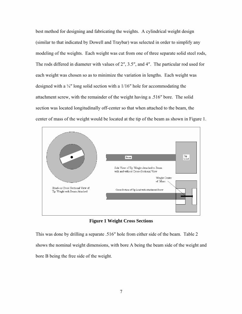
best method for designing and fabricating the weights. A cylindrical weight design
(similar to that indicated by Dowell and Traybar) was selected in order to simplify any
modeling of the weights. Each weight was cut from one of three separate solid steel rods,
The rods differed in diameter with values of 2″, 3.5″, and 4″. The particular rod used for
each weight was chosen so as to minimize the variation in lengths. Each weight was
designed with a ¼″ long solid section with a 1/16″ hole for accommodating the
attachment screw, with the remainder of the weight having a .516″ bore. The solid
section was located longitudinally off-center so that when attached to the beam, the
center of mass of the weight would be located at the tip of the beam as shown in Figure 1.
Figure 1 Weight Cross Sections
This was done by drilling a separate .516″ hole from either side of the beam. Table 2
shows the nominal weight dimensions, with bore A being the beam side of the weight and
bore B being the free side of the weight.
7

Table 2 Tip Weight Dimensions
Designed Weight (lb)
Diameter (in)
Total Length (in)
Bore A Length (in)
Bore B Length (in)
Actual Weight (lb)
0.5 2 0.939 0.633 0.056 0.491 2 1.158 0.588 0.320 1.01
1.5 2 3.471 1.899 1.322 1.502 3.5 0.727 0.366 0.111 2.013 3.5 1.094 0.550 0.294 3.024 4 1.112 0.733 0.129 4.01
4.5 4 1.251 0.824 0.177 4.52
The 0.5 and 1.5 lb weights were manufactured for a wider beam with 1.505″ diameter
bores, but were otherwise identical in nature to the rest of the weights, which are depicted
in Figure 2.
Figure 2 Tip Weights
The weights were fixed to the beam using a 1/16″ screw.
Each weight’s moments of inertia were calculated using the following equations:
Ixx = ½*MA*(RiA2+Ro
2) + ½*MB*(RB iB2+Ro
2) + ½*MS*(RiC2+Ro
2) (1)
Iyy = Izz = 1/12*MALA2+MA*dA
2 + 1/12*MBLB B2+MBB*dB
2 + 1/12*MSLS2+MS*dS
2 (2)
8
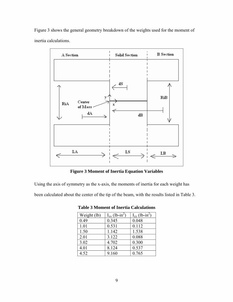
Figure 3 shows the general geometry breakdown of the weights used for the moment of
inertia calculations.
Figure 3 Moment of Inertia Equation Variables
Using the axis of symmetry as the x-axis, the moments of inertia for each weight has
been calculated about the center of the tip of the beam, with the results listed in Table 3.
Table 3 Moment of Inertia Calculations
Weight (lb) Ixx (lb-in2) Iyy (lb-in2) 0.49 0.345 0.048 1.01 0.531 0.112 1.50 1.142 1.538 2.01 3.122 0.088 3.02 4.702 0.300 4.01 8.124 0.537 4.52 9.160 0.765
9

Set-Up
The beam was clamped to the swivel attachment with a cover plate and four ¼″
diameter bolts, so that 30″ of beam extended past the clamp point. The swivel attachment
was then bolted to a rod fixture using two ¼″ diameter bolts. The rod fixture was
clamped to a fixation rod with two ½″ diameter bolts. The fixation rod was bolted in
place on a vibration isolation table by four ¼″ diameter bolts. This set-up can be seen in
Figure 4 for the zero degree pitch case.
x
y
zo
Figure 4 Swivel Attachment The swivel attachment allowed for 360 degree pitch rotation of the beam between trial
runs, while fixing the beam in place for each trial. The base of the beam where it attaches
to the swivel attachment is considered the origin, with positive length measurement going
10

toward the end of the beam where the tip weights attach. The directional and pitch
terminology is shown in Figure 5.
Figure 5 Directional Orientation
The pitch angle was set and measured using an SPI Protracto Level II Inclinometer. Pitch
angle refers to the beam pitch angle at the root where it is held by the swivel attachment.
Accelerometers
For the frequency determination portion of the experiment, an accelerometer was
mounted in each of three locations. Each accelerometer was a PCB Piezotronics model
number 352C22, weighing 0.5 grams (0.0011 pounds). The combined weight of the
accelerometers was only 1.8% of the unloaded beam weight (0.182 lb) and less than 0.5%
11

of the lowest loaded beam weight, making their contribution negligible. One was placed
at 28″, centered on the wide side of the beam to measure the flapwise frequency. One
was placed at 28.25″, off-center on the wide side of the beam to measure the flapwise
frequency and identify/eliminate rotational frequencies. One was placed at 29″, centered
on the narrow side of the beam to measure the chordwise frequency. This arrangement is
illustrated in Figure 4.
Figure 6 Accelerometer Locations
The beam was manually excited simultaneously in the flapwise and chordwise directions.
This was done by striking the beam off center at the midspan by finger, simulating an
impulse force. The accelerometers were attached to a SignalCalc Savant Dynamic Signal
Analyzer operating with SigCalc 720 software which used a Fourier Transform routine to
convert the time data into frequency data. The natural frequencies were identified in the
frequency domain by large rises in output value. The software was set to average 5 data
sets with a 90% overlap, a frequency span of 20 Hz (40 Hz sampling rate), a time span of
160 seconds, and a Hanning window. These settings allowed for a measurement
accuracy of +/-0.0038 Hz in the flapwise direction and +/-0.0084 Hz in the chordwise.
By contrast, the Princeton Beam Experiment at best allowed for a frequency
measurements accuracy of +/-0.1012 Hz in the flapwise direction and +/-0.0617 Hz in the
12

chordwise. During this portion, only the first natural frequency was recorded for each
direction (flapwise and chordwise).
Laser Vibrometer
For the mode shape portion of the experiment, the Polytec Scanning Vibrometer
PSV 400-3D with software version 8.2 was used to measure velocity data which was then
converted into normalized mode shape data. Hi-Vi Research Model F6, 60 Watt, 8 ohm
speaker was used to excite the root end of the beam in the desired direction. To create
steady state data, the speaker was set to excite the beam at the specific frequency of
interest and allowed to act on the beam for several minutes prior to scanning. The
speaker input amplitude was set to ten volts-peak-to-peak (VPP) for frequencies below 10
Hz and 5 VPP for frequencies above 10 Hz. The laser vibrometer scanned the beam,
measuring velocity values at each of 25 predetermined points along the neutral axis, and
combined this data with the input signal to the speaker to record phase and peak velocity
data at the desired frequency. The velocity and phase data was then used to plot the
mode shapes. This set-up is depicted in Figure 7.
13

Figure 7 Scanning Laser Vibrometer Set-up
Attempts were made at creating two and three dimensional grids; however, this
could not be done for a sufficiently large portion of the beam due to limitations of the
laser vibrometer, unavailable static measurements and the length/slenderness ratio of the
beam. Specifically, the 60 to 1 length to height ratio forced the camera to be zoomed out
to the point where automatic alignment for multi-dimensional grids was not possible as
the minimum separation between alignment points forced them to be separated by more
than the width of the beam. Manual alignment of the equipment for multi-dimensional
grids requires exact static measurements of the loaded system. The unavailability of this
data eliminated manual alignment as an option. Consequently, only the one dimensional
measurements were made.
The scanning laser vibrometer was also used to determine higher order natural
frequency values in the chordwise direction. For these tests the desire was only to
identify the desired frequencies and then use the previously mentioned set-up to
14

determine the mode shapes. The set-up was similar to that described above, with a few
differences intended to either decrease testing time or allowing for frequency
identification over a range of values. First, the speaker was set to excite the beam over a
large range of frequencies (0 to 256 Hz), rather than just the desired frequency. Second,
only five scan points were used, this significantly decreased the testing time while only
eliminating mode shape data which would be captured in subsequent testing. Last, the
laser vibrometer software was set to display the frequency response of the system using a
Fourier transform routine which was then used to identify the second and third natural
frequencies.
Instrumentation Choices
The laser vibrometer was initially considered the preferred data collection method
due to its ability to collect data along the entire length of the beam; however, it has three
limitations which necessitated the use of accelerometer measurements. First, the laser
vibrometer software limits open frequency scan resolution to +/- 0.0156 Hz. Since the
first natural chordwise frequencies occur below 1 Hz, this leads to measurement errors as
great as 14% for the first mode; whereas, the accelerometers allowed for the
determination of the natural frequencies to within +/- 0.0038 Hz (0.05-0.77% chordwise
error, 0.09-1.41% flapwise error). Second, once pitch is introduced, the set-up
requirements become extremely time consuming and the laser has a hard time reflecting
back to the vibrometer. Third, geometrical angle limitations coupled with the narrow
width of the beam made it impossible to acquire flapwise frequency data along the entire
beam length in a single trial run.
15

III. Results and Analysis
Differences in Methodology
A few differences in techniques and methodology may contribute to the small
differences in data recorded in this experiment versus the Princeton Beam data. Dowell
and Traybar claim to have an error in frequency reading of only +/-0.1% [1:5], however
in several cases multiple readings were taken for the same set-up with a difference in
measurement as high as 2.53% and they made no allowance for instrumentation error or
repeatability error. Additionally, the fixture holding the beam root used by Dowell and
Traybar could not be reproduced, so a different one described previously was used. The
Princeton Beam Experiment documentation lists all load weights as whole number values
and all angle measurement are listed as exact whole numbers in five degree increments,
with the precision of these measurements left unknown. The new data is taken with an
angle measurement precision of 0.1 degree and a weight measurement precision of 0.01
lb. Additionally, the angle setting limitations of the swivel attachment made getting
closer than one degree to a desired angle very difficult; producing some small differences
in data points. The Princeton Beam data was derived from measurements taken at the
blade root, rather than the blade tip which increases the associated precision error as a
result of the smaller amplitudes for the first natural frequency. Finally, the
instrumentation used in the Princeton experiment consisted of glued-on strain gages
(circa 1975) which introduces more stiffness than the lightweight accelerometers used in
16
this experiment; thus causing a small, but not necessarily inconsequential increase in the
measured frequencies.
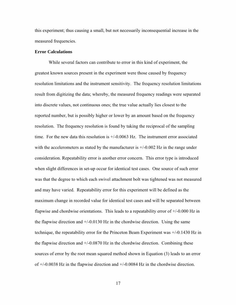
Error Calculations
While several factors can contribute to error in this kind of experiment, the
greatest known sources present in the experiment were those caused by frequency
resolution limitations and the instrument sensitivity. The frequency resolution limitations
result from digitizing the data; whereby, the measured frequency readings were separated
into discrete values, not continuous ones; the true value actually lies closest to the
reported number, but is possibly higher or lower by an amount based on the frequency
resolution. The frequency resolution is found by taking the reciprocal of the sampling
time. For the new data this resolution is +/-0.0063 Hz. The instrument error associated
with the accelerometers as stated by the manufacturer is +/-0.002 Hz in the range under
consideration. Repeatability error is another error concern. This error type is introduced
when slight differences in set-up occur for identical test cases. One source of such error
was that the degree to which each swivel attachment bolt was tightened was not measured
and may have varied. Repeatability error for this experiment will be defined as the
maximum change in recorded value for identical test cases and will be separated between
flapwise and chordwise orientations. This leads to a repeatability error of +/-0.000 Hz in
the flapwise direction and +/-0.0130 Hz in the chordwise direction. Using the same
technique, the repeatability error for the Princeton Beam Experiment was +/-0.1430 Hz in
the flapwise direction and +/-0.0870 Hz in the chordwise direction. Combining these
sources of error by the root mean squared method shown in Equation (3) leads to an error
of +/-0.0038 Hz in the flapwise direction and +/-0.0084 Hz in the chordwise direction.
17
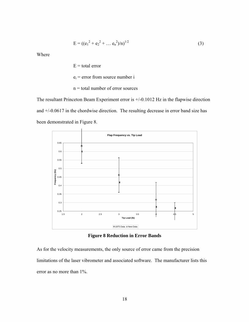
E = ((e12 + e2
2 + … en2)/n)1/2 (3)
Where
E = total error
ei = error from source number i
n = total number of error sources
The resultant Princeton Beam Experiment error is +/-0.1012 Hz in the flapwise direction
and +/-0.0617 in the chordwise direction. The resulting decrease in error band size has
been demonstrated in Figure 8.
Flap Frequency vs. Tip Load
0.25
0.3
0.35
0.4
0.45
0.5
0.55
0.6
0.65
1.5 2 2.5 3 3.5 4 4.5 5
Tip Load (lb)
Freq
uenc
y (H
z)
1975 Data New Data Figure 8 Reduction in Error Bands
As for the velocity measurements, the only source of error came from the precision
limitations of the laser vibrometer and associated software. The manufacturer lists this
error as no more than 1%.
18
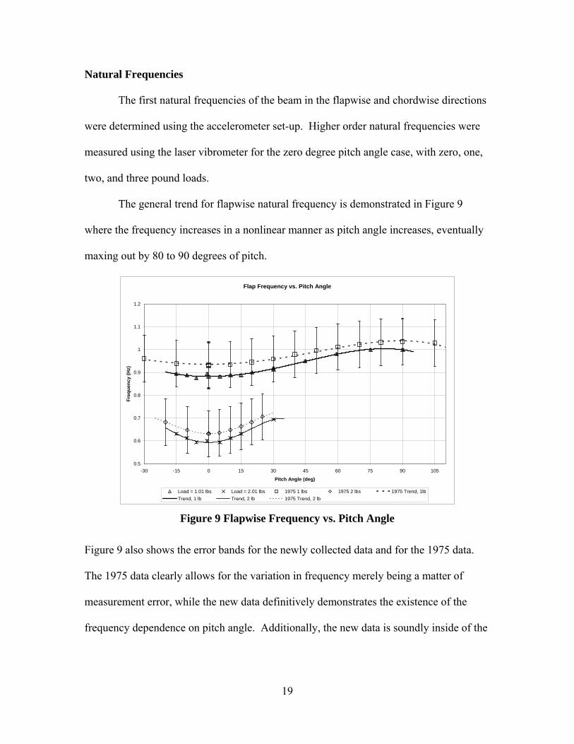
Natural Frequencies
The first natural frequencies of the beam in the flapwise and chordwise directions
were determined using the accelerometer set-up. Higher order natural frequencies were
measured using the laser vibrometer for the zero degree pitch angle case, with zero, one,
two, and three pound loads.
The general trend for flapwise natural frequency is demonstrated in Figure 9
where the frequency increases in a nonlinear manner as pitch angle increases, eventually
maxing out by 80 to 90 degrees of pitch.
Flap Frequency vs. Pitch Angle
0.5
0.6
0.7
0.8
0.9
1
1.1
1.2
-30 -15 0 15 30 45 60 75 90 105
Pitch Angle (deg)
Freq
uenc
y (H
z)
Load = 1.01 lbs Load = 2.01 lbs 1975 1 lbs 1975 2 lbs 1975 Trend, 1lbTrend, 1 lb Trend, 2 lb 1975 Trend, 2 lb Figure 9 Flapwise Frequency vs. Pitch Angle
Figure 9 also shows the error bands for the newly collected data and for the 1975 data.
The 1975 data clearly allows for the variation in frequency merely being a matter of
measurement error, while the new data definitively demonstrates the existence of the
frequency dependence on pitch angle. Additionally, the new data is soundly inside of the
19

error bands from the Princeton Beam Experiment and follows the same trend, providing a
high degree of confidence in the results.
The general trend for chordwise natural frequency is demonstrated in Figure 10
where the frequency decreases in a nonlinear manner as pitch angle increases, reaching a
minimum between 80 and 90 degrees of pitch.
Chord Frequency vs. Pitch Angle
2
2.2
2.4
2.6
2.8
3
3.2
3.4
3.6
3.8
4
-30 -15 0 15 30 45 60 75 90 105
Pitch Angle (deg)
Freq
uenc
y (H
z)
Load = 1.01 lbs Load = 2.01 lbs 1975 1 lbs 1975 2 lbs 1975 Trend, 1 lbTrend 1 lb 1975 Trend, 2 lb Trend, 2 lb
Figure 10 Chordwise Frequency vs. Pitch Angle
These trends in frequency versus pitch angle match the Princeton Beam Experiment and
remained consistent for all tip weight values. It is notable that the new data falls outside
of the error bands from the Princeton Beam Experiment. Part of the reason for this is that
the error bars from the Princeton Beam experiment have been made estimates of the error
30 years after the experiment was performed and those estimates represent absolute
minimums and are likely to be smaller than the true error bars. Additionally, differences
in methodology previously mentioned have contributed to a small difference in the
20

solution, specifically, the stiffening affect of the strain gages in the Princeton Beam
Experiment and failure to account for the presence of higher order modes raised the
measured values with respect to the uninstrumented (true) values.
It should be noted that in both the flapwise and chordwise directions the new
measurements average 5.7% lower (standard deviation of 3.3%) for the same test
conditions. This disparity is mostly likely the result of the differences in experimental
set-up mentioned previously. Additionally, the small changes in pitch angle used for test
points can have a significant impact on the frequencies for the heavy tip loads.
Specifically, when the 4.5 lb weight was applied with -0.8 degrees of pitch, the total twist
of 17 degrees is reached by the end of the beam; on the other hand, a zero degree pitch
should have resulted in no twist at all. This is a large part of the reason why the 4.5 lb
weight registered a noticeably higher flapwise frequency than the Princeton Beam
Experiment.
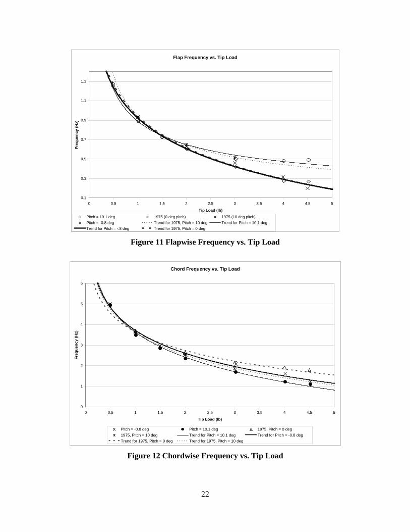
When the frequency changes are tracked versus tip load, the result is a nonlinear
decrease which closely matches the results found in the Princeton Beam Experiment. A
comparison of the new data with the 1975 data for frequency vs. tip load can be found in
Figure 11 and Figure 12.
21
Flap Frequency vs. Tip Load
0.1
0.3
0.5
0.7
0.9
1.1
1.3
0 0.5 1 1.5 2 2.5 3 3.5 4 4.5 5
Tip Load (lb)
Freq
uenc
y (H
z)
Pitch = 10.1 deg 1975 (0 deg pitch) 1975 (10 deg pitch)Pitch = -0.8 deg Trend for 1975, Pitch = 10 deg Trend for Pitch = 10.1 degTrend for Pitch = -.8 deg Trend for 1975, Pitch = 0 deg
Figure 11 Flapwise Frequency vs. Tip Load
Chord Frequency vs. Tip Load
0
1
2
3
4
5
6
0 0.5 1 1.5 2 2.5 3 3.5 4 4.5
Tip Load (lb)
Freq
uenc
y (H
z)
5
Pitch = -0.8 deg Pitch = 10.1 deg 1975, Pitch = 0 deg1975, Pitch = 10 deg Trend for Pitch = 10.1 deg Trend for Pitch = -0.8 degTrend for 1975, Pitch = 0 deg Trend for 1975, Pitch = 10 deg
Figure 12 Chordwise Frequency vs. Tip Load
22

Trend lines have been added to the figures to simplify the comparison. The trend lines
use a power series method to determine a line which most closely matches the associated
data, these lines are not necessarily the correct equations for the experimental set-up,
rather they represent data matching and are used for comparison purposes only.
Mode Shapes
Consistent mode shape data was only obtainable in the flapwise direction at 0
degrees pitch. The data was taken by recording the peak velocity output at known
locations on the beam centerline and normalizing it. The beam length was normalized by
dividing the data point length coordinate by the total beam length (x/L). The velocity
data was normalized by dividing the velocity recorded at each data point by the
maximum velocity recorded for the mode shape in question, so that the peak value
becomes +/-1. Since acceleration, velocity and displacement data differ only by constant
multipliers, dependent on the test frequency, the normalized data can be interpreted as
representing the displacement, velocity, and acceleration variation along the beam. The
Princeton Beam Experiment did not seek to identify mode shape data; therefore, the data
will be compared to linear theory as, developed in Appendix B, to show general form
agreement, recognizing that the reason experimental data of this nature is needed is that
linear theory cannot be applied to the high load limits of rotor blades. The linear theory
results will be calculated at the zero pound load case and the infinite pound load case.
The infinite load case represents the solution with a tip load weighing 1011 pounds which
while not truly infinite, is sufficiently large compared to the beam weight as to
approximate an infinite load case.
23

Figure 13 depicts the first mode shape as compared to linear theory.
Mode 1
0
0.1
0.2
0.3
0.4
0.5
0.6
0.7
0.8
0.9
1
0 0.1 0.2 0.3 0.4 0.5 0.6 0.7 0.8 0.9 1
Beam Position (x/L)
Nor
mal
ized
Vel
ocity
Linear Theory (0 lb) Linear Theory (infinite load) no load 1 lb 2 lb 3 lb Figure 13 Flapwise Mode 1
It is evident that for this particular set of weights and zero pitch, that linear mode shape
theory predicts the correct approximate shape for the first mode. This is not surprising in
that the data has been normalized to a maximum magnitude of one and the primary
difference for the first mode from the linear to the nonlinear range should be their relative
magnitude.
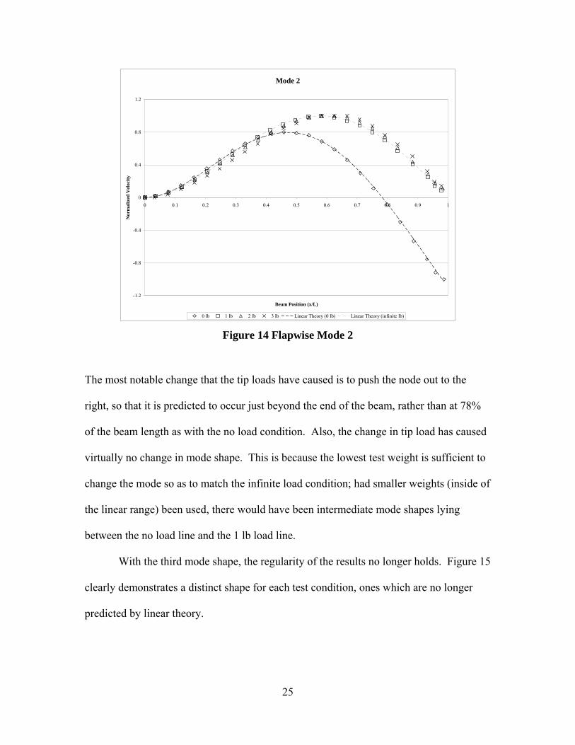
The second mode shape also closely matched linear theory as shown in Figure 14.
24
Mode 2
-1.2
-0.8
-0.4
0
0.4
0.8
1.2
0 0.1 0.2 0.3 0.4 0.5 0.6 0.7 0.8 0.9 1
Beam Position (x/L)
Nor
mal
ized
Vel
ocity
0 lb 1 lb 2 lb 3 lb Linear Theory (0 lb) Linear Theory (infinite lb) Figure 14 Flapwise Mode 2
The most notable change that the tip loads have caused is to push the node out to the
right, so that it is predicted to occur just beyond the end of the beam, rather than at 78%
of the beam length as with the no load condition. Also, the change in tip load has caused
virtually no change in mode shape. This is because the lowest test weight is sufficient to
change the mode so as to match the infinite load condition; had smaller weights (inside of
the linear range) been used, there would have been intermediate mode shapes lying
between the no load line and the 1 lb load line.
With the third mode shape, the regularity of the results no longer holds. Figure 15
clearly demonstrates a distinct shape for each test condition, ones which are no longer
predicted by linear theory.
25

Mode 3
-1.5
-1
-0.5
0
0.5
1
1.5
0 0.2 0.4 0.6 0.8 1 1.2
Beam Position (x/L)
Nor
mal
ized
Vel
ocity
0 lb 1 lb 2 lb 3 lb Linear Theory (0 lb) Linear Theory (infinite lb) Figure 15 Flapwise Mode 3
For each tip load case, the nodes have both been shifted rightward. In fact, with the three
pound weight, the second node has almost shifted to the end of the beam. A large part of
the reason for the rightward shift in the node locations is that the tip load at the end of the
beam is significantly heavier than the beam itself. Even the 1 lb load is 5.67 times the
weight of the beam. As a result of the weight disparity, the tip loads act as inertial
dampers, attempting to keep the end of the beam from moving at the higher frequencies.
Thus the beam with the heaviest load acts like a fixed-fixed beam excited at the first
mode, rather than a cantilever beam excited at the third mode. This inertial damping
effect is not accounted for by linear theory.
26
IV. Conclusions and Recommendations
Accelerometer Results
The accelerometer results greatly improved upon those of the Princeton Beam
Experiment. The natural frequency results fell within the error bands from the Princeton
Beam Experiment and the error band sizes were reduced by an order of magnitude. This
data used time averaging of several overlapping tests while the Princeton Beam
Experiment used singular test results. The beam instrumentation accounted for the
presence of higher order modes and separated them from the desired modes while the
Princeton data makes no allowance for higher order modes. The new data points were
selected at equal angular increments for each load case, making it more useable than the
prior data. The experimental process has been sufficiently documented as to be
replicated and modeled by others, which was the greatest shortcoming of the Princeton
Beam data. All the natural frequency data collected followed the same trends and fell
within the limits established by past experimentation while at the same time reducing
several sources of error, making the data more reliable than the Princeton Beam
Experiment data.
Laser Vibrometer Results
There is no baseline of comparison for the laser vibrometer results. This
experiment was performed to measure mode shapes outside of the linear range and no
similar experimentation has been identified. Complex nonlinear models were not
available for comparison. This is the reason that measurements were taken for the
27
unloaded case as well as the loaded cases. The unloaded results match closely with
theoretical results which have been validated and documented in numerous texts. Since
the experimental process used for both unloaded and loaded cases was identical, the
results from the loaded cases are at least as good as the unloaded results. The mode
shapes graphed in the results sections accurately reflect the actual mode shapes
experienced by the beam.
Laser Vibrometer Evaluation
The laser vibrometer use was limited by a number of problems which may be
avoidable in future experimentation. The greatest limitations were related to frequency
resolution, beam geometry, deformation extent, and a lack of static data. At the same
time it provided a great deal of data which could not have otherwise been obtained.
Frequency Resolution
The laser vibrometer used for this experiment is limited to a frequency resolution
of +/-0.01562 Hz while scanning to detect natural frequency values. For this particular
experiment, the resulting error in measured natural frequencies would have been as great
as 5.8% and averaged 2% in the flapwise (worst case) direction. On the other hand, the
accelerometer set-up has no such resolution limit and can be made to measure with as
fine a resolution as desired; however, the trade off is an ever increasing experimental
time required to meet the desired resolution. For simplicity, the same settings were used
for all accelerometer tests; these settings led to a maximum frequency error of 2.3% and
average error of 0.7% for the flapwise direction. Table 4 shows the minimum frequency
value detectable for a given maximum desired error for both the laser vibrometer and the
accelerometer (as used in the experiment). What this amounts to is that the laser
28

vibrometer is not very accurate in determining natural frequencies below 1.25 Hz. For
future considerations, use of a beam which is shorter, more rigid, thicker, or otherwise
designed to have a higher first natural frequency would allow for the entire experiment to
be performed using only the laser vibrometer.
Table 4 Frequency Limitations
Laser Vibrometer Minimum Detectable Frequency (Hz)
Accelerometer Minimum Detectable Frequency (Hz)
Maximum Error (%)
6.25 15.625 0.11.25 3.125 0.5
0.625 1.5625 10.125 0.3125 5
0.0625 0.15625 10
Twist
The laser vibrometer requires that the laser beam be reflected back to the
vibrometer in order for measurements to be made. With the 30″ beam used in this
experiment, a tip load of one pound with a pitch of only ten degrees caused sufficient
twist in the beam as to stop the laser from reflecting back to the vibrometer along large
portions of the beam, making modal mapping impossible. In the future this problem may
be avoidable with a structure that either twists less severely or a surface which provides
better beam reflection.
Static Measurements
The laser vibrometer is capable of performing up a three dimensional analysis of a
specimen; however, this requires a static mapping of the structure for each test case.
Obtaining the static measurements for all test cases prior to dynamic testing would allow
for the creation of substantially improved mode shape mapping.
29

Beam Geometry
The length of the beam required it to be placed two meters from the laser
vibrometer in order to capture data along the entire length. This distance requirement,
coupled with the narrow flapwise side of the beam and the need for reasonable beam
angles, made it impossible to capture mode shape data in the chordwise direction. In fact,
attempts were made to capture chordwise data along only half the length of the beam at
zero degree pitch angle, but the 1/8″ surface proved too small to collect data over longer
than a 2″ span in any single run. Using a shorter, thicker specimen in the future may
make it possible to capture this additional information.
Benefits
There were several benefits to using the laser vibrometer. The laser vibrometer
allowed for the relatively simple determination of mode shapes. Without this equipment,
mode shapes would be virtually indeterminate. The laser vibrometer requires absolutely
no instrumentation to be mounted on the test specimen; thus the specimen characteristics
are left unaffected by the equipment. Accounting for the problems mentioned above
would allow for the creation of a three dimensional model of a specimen which can
determine the natural mode shapes and frequencies across a large spectrum range in a
single scan.
Future Experimentation
Several matters presented themselves which would be of interest for future study.
No torsional analysis was performed; however there was clearly a torsional element
present, particularly with the heavier weights. The first torsional mode decreased by at
30
least one order of magnitude between the 1/2 lb load condition and the 4.5 lb load
condition. The first torsional frequency also displayed a visible dependence on pitch
angle. At the third mode shape, the beam was beginning to act more like a fixed-fixed
beam than a cantilever beam; it would be interesting to determine if this continues to
happen with higher order modes.
Ultimately, future experimentation would be greatly aided by using a specimen
which is shorter, stiffer, thicker, and/or possessing of a first natural frequency of at least
1.25 Hz. Even without such adjustments, the experimental process laid out in this report
lead to accurate measurements of natural frequencies and mode shapes for cantilever type
beams.
31

Appendix A. Data
Table 5 Accelerometer Data
Trial # Tip Load (lb) Pitch (deg) Flapwise
Frequency (Hz) Chordwise
Frequency (Hz) 1 1.01 0.02 0.8812 3.5382 1.01 10.14 0.8875 3.53 1.01 20.12 0.9 3.44 1.01 30.03 0.9187 3.2885 0.49 -0.8 1.275 4.9946 1.01 -0.8 0.8937 3.5567 1.5 -0.8 0.725 2.9568 2.01 -0.8 0.6 2.5319 3.02 -0.8 0.4187 2.075
10 4.01 -0.8 0.275 1.61911 4.52 -0.8 0.2688 1.21912 0 -0.8 4.213 16.3113 0 5.18 4.288 16.3814 0.49 5.18 1.256 4.96215 1.01 5.18 0.8812 3.54416 2.01 5.18 0.5937 2.517 1.5 5.18 0.7187 2.93818 3.02 5.18 0.4375 1.91319 4.01 5.18 0.3875 1.33820 4.52 5.18 0.4125 1.13721 4.52 5.18 0.4125 1.14422 0 -5.8 4.194 16.3623 0.49 -5.8 1.256 4.97524 1.01 -5.8 0.875 3.53125 2.01 -5.8 0.5937 2.45626 3.02 -5.8 0.45 1.88127 4.01 -5.8 0.3937 1.38828 4.52 -5.8 0.425 1.12529 1.5 -5.8 0.7187 2.91930 1.5 -10.1 0.725 2.81931 0 -10.1 4.175 16.4732 0.49 -10.1 1.25 4.9533 1.01 -10.1 0.8875 3.53134 2.01 -10.1 0.6125 2.36935 3.02 -10.1 0.5 1.706
32

Trial # Tip Load (lb) Pitch (deg) Flapwise
Frequency (Hz) Chordwise
Frequency (Hz) 36 4.01 -10.1 0.4687 1.26937 4.52 -10.1 0.4875 1.09438 1.5 -15 0.7375 2.78839 0 -15 4.113 16.4840 0.49 -15 1.256 4.94441 1.01 -15 0.8937 3.46342 2.01 -15 0.6312 2.25643 3.02 -15 0.5437 1.58844 3.02 15.04 0.55 1.56945 2.01 15.04 0.6312 2.2546 1.5 15.04 0.7375 2.78147 1.01 15.04 0.8875 3.45648 0.49 15.04 1.256 4.92549 0 15.04 4.181 16.4850 0 30.1 4.131 16.5151 0 30.1 4.131 16.5152 0.49 30.1 1.256 4.87553 1.01 30.1 0.9125 3.31354 2.01 30.1 0.6937 2.01955 1.5 30.1 0.775 2.56956 1.5 44.8 0.8312 2.457 1.01 44.8 0.95 3.14458 0.49 44.8 1.269 4.78759 0 44.8 4.3 16.3960 0 59.4 4.194 16.4461 0.49 59.4 1.288 4.70662 1.01 59.4 0.9812 3.04463 1.5 59.4 0.8687 2.31964 0 75.19 4.119 16.4965 0.49 75.19 1.294 4.6566 1.01 75.19 1 2.96367 1.01 90.1 1 2.94468 0.49 90.1 1.306 4.63169 0 90.1 4.138 16.4670 0.49 10.1 1.256 4.93171 4.52 10.1 0.4937 1.08772 4.01 10.1 0.4812 1.21373 3.02 10.1 0.5 1.69474 2.01 10.1 0.6125 2.34475 1.5 10.1 0.725 2.83876 1.01 10.1 0.8875 3.488
33

Trial # Tip Load (lb) Pitch (deg) Flapwise
Frequency (Hz) Chordwise
Frequency (Hz) 77 0.49 10.1 1.256 4.94478 0 10.1 4.138 16.44
Table 6 Princeton Beam Data [1:46-50] (Included for Reference)
Tip Load (lb) Pitch (deg) Flap Frequency (Hz) Chord Frequency (Hz) 0 0 4.475 17.2170 0 4.607 17.2130 0 4.49 17.1710 0 17.1740 0 17.2070 0 4.464 17.2581 -105 1.033 3.1381 -90 3.1221 -90 1.034 3.121 -75 1.028 3.1351 -60 1.011 3.1991 -45 0.99 3.2981 -30 0.961 3.4431 -15 0.939 3.5911 0 0.932 3.6981 0 3.6471 0 0.935 3.6621 0 0.928 3.6741 10 0.935 3.6171 20 0.945 3.5411 30 0.96 3.4481 35 3.3941 40 0.979 3.3541 50 0.997 3.2771 60 1.012 3.2151 70 1.023 3.1751 80 1.032 3.1451 90 1.035 3.1431 90 1.033 3.1381 105 1.029 3.1552 -20 0.682 2.3152 -10 0.648 2.5172 0 0.632 2.6292 0 0.631 2.637
34
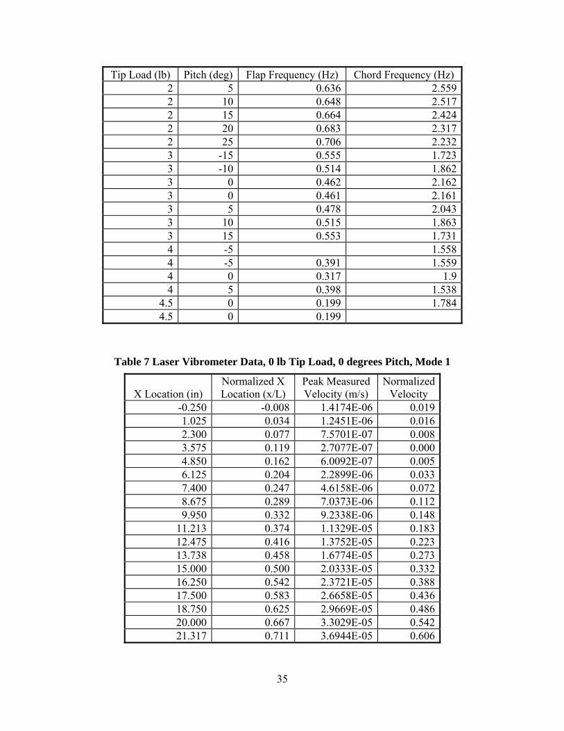
Tip Load (lb) Pitch (deg) Flap Frequency (Hz) Chord Frequency (Hz) 2 5 0.636 2.5592 10 0.648 2.5172 15 0.664 2.4242 20 0.683 2.3172 25 0.706 2.2323 -15 0.555 1.7233 -10 0.514 1.8623 0 0.462 2.1623 0 0.461 2.1613 5 0.478 2.0433 10 0.515 1.8633 15 0.553 1.7314 -5 1.5584 -5 0.391 1.5594 0 0.317 1.94 5 0.398 1.538
4.5 0 0.199 1.7844.5 0 0.199
Table 7 Laser Vibrometer Data, 0 lb Tip Load, 0 degrees Pitch, Mode 1
X Location (in) Normalized X Location (x/L)
Peak Measured Velocity (m/s)
Normalized Velocity
-0.250 -0.008 1.4174E-06 0.019 1.025 0.034 1.2451E-06 0.016 2.300 0.077 7.5701E-07 0.008 3.575 0.119 2.7077E-07 0.000 4.850 0.162 6.0092E-07 0.005 6.125 0.204 2.2899E-06 0.033 7.400 0.247 4.6158E-06 0.072 8.675 0.289 7.0373E-06 0.112 9.950 0.332 9.2338E-06 0.148
11.213 0.374 1.1329E-05 0.183 12.475 0.416 1.3752E-05 0.223 13.738 0.458 1.6774E-05 0.273 15.000 0.500 2.0333E-05 0.332 16.250 0.542 2.3721E-05 0.388 17.500 0.583 2.6658E-05 0.436 18.750 0.625 2.9669E-05 0.486 20.000 0.667 3.3029E-05 0.542 21.317 0.711 3.6944E-05 0.606
35

X Location (in) Normalized X Location (x/L)
Peak Measured Velocity (m/s)
Normalized Velocity
22.633 0.754 4.1328E-05 0.679 23.950 0.798 4.5481E-05 0.748 25.267 0.842 4.9142E-05 0.808 26.583 0.886 5.2700E-05 0.867 27.900 0.930 5.5963E-05 0.921 28.750 0.958 5.8711E-05 0.966 29.600 0.987 6.0750E-05 1.000
Table 8 Laser Vibrometer Data, 0 lb Tip Load, 0 degrees Pitch, Mode 2
X Location (in) Normalized X Location (x/L)
Peak Measured Velocity (m/s)
Normalized Velocity
-0.250 -0.008 1.1461E-04 0.000 1.025 0.034 5.3323E-04 0.020 2.300 0.077 1.5673E-03 0.070 3.575 0.119 3.1850E-03 0.148 4.850 0.162 5.1853E-03 0.245 6.125 0.204 7.4725E-03 0.356 7.400 0.247 9.7621E-03 0.466 8.675 0.289 1.1949E-02 0.572 9.950 0.332 1.3844E-02 0.664
11.213 0.374 1.5369E-02 0.738 12.475 0.416 1.6313E-02 0.783 13.738 0.458 1.6649E-02 0.799 15.000 0.500 1.6456E-02 0.790 16.250 0.542 1.5866E-02 0.762 17.500 0.583 1.4379E-02 0.690 18.750 0.625 1.2337E-02 0.591 20.000 0.667 9.6408E-03 0.461 21.317 0.711 6.2989E-03 0.299 22.633 0.754 2.4890E-03 0.115 23.950 0.798 1.9169E-03 -0.087 25.267 0.842 6.3166E-03 -0.300 26.583 0.886 1.1172E-02 -0.535 27.900 0.930 1.5735E-02 -0.755 28.750 0.958 1.9113E-02 -0.919 29.600 0.987 2.0798E-02 -1.000
36

Table 9 Table 5 Laser Vibrometer Data, 0 lb Tip Load, 0 degrees Pitch, Mode 3
X Location (in) Normalized X Location (x/L)
Peak Measured Velocity (m/s)
Normalized Velocity
-0.300 -0.010 1.2699E-03 0.014 1.025 0.034 4.1388E-03 0.070 2.350 0.078 1.0788E-02 0.198 3.675 0.123 1.9880E-02 0.373 5.000 0.167 2.9268E-02 0.555 6.250 0.208 3.7096E-02 0.706 7.500 0.250 4.2070E-02 0.802 8.750 0.292 4.3382E-02 0.827
10.000 0.333 4.0732E-02 0.776 11.238 0.375 3.4431E-02 0.654 12.475 0.416 2.5078E-02 0.474 13.713 0.457 1.3441E-02 0.249 14.950 0.498 5.3124E-04 0.000 16.213 0.540 1.2400E-02 -0.229 17.475 0.583 2.3799E-02 -0.449 18.738 0.625 3.2345E-02 -0.614 20.000 0.667 3.6952E-02 -0.703 21.250 0.708 3.7084E-02 -0.705 22.500 0.750 3.2882E-02 -0.624 23.750 0.792 2.4269E-02 -0.458 25.000 0.833 1.0666E-02 -0.196 26.525 0.884 8.0406E-03 0.145 28.050 0.935 2.7609E-02 0.523 28.875 0.963 4.3372E-02 0.827 29.700 0.990 5.2345E-02 1.000
Table 10 Table 5 Laser Vibrometer Data, 1 lb Tip Load, 0 degrees Pitch, Mode 1
X Location (in) Normalized X Location (x/L)
Peak Measured Velocity (m/s)
Normalized Velocity
-0.200 -0.007 1.1557E-06 0.000 1.088 0.036 4.0992E-06 0.004 2.375 0.079 1.1724E-05 0.015 3.663 0.122 2.4077E-05 0.033 4.950 0.165 4.0614E-05 0.057 6.188 0.206 6.0604E-05 0.086 7.425 0.248 8.4086E-05 0.120 8.663 0.289 1.1076E-04 0.158 9.900 0.330 1.3893E-04 0.199
37

X Location (in) Normalized X Location (x/L)
Peak Measured Velocity (m/s)
Normalized Velocity
11.150 0.372 1.6933E-04 0.243 12.400 0.413 2.0203E-04 0.290 13.650 0.455 2.3583E-04 0.339 14.900 0.497 2.7064E-04 0.389 16.175 0.539 3.0822E-04 0.443 17.450 0.582 3.4825E-04 0.501 18.725 0.624 3.8635E-04 0.556 20.000 0.667 4.2376E-04 0.610 21.250 0.708 4.6008E-04 0.663 22.500 0.750 4.9571E-04 0.714 23.750 0.792 5.3010E-04 0.764 25.000 0.833 5.6760E-04 0.818 26.500 0.883 6.1489E-04 0.886 28.000 0.933 6.5442E-04 0.943 28.675 0.956 6.7393E-04 0.972 29.350 0.978 6.9364E-04 1.000
Table 11 Table 5 Laser Vibrometer Data, 1 lb Tip Load, 0 degrees Pitch, Mode 2
X Location (in) Normalized X Location (x/L)
Peak Measured Velocity (m/s)
Normalized Velocity
-0.200 -0.007 2.7907E-04 0.000 1.088 0.036 1.0796E-03 0.019 2.375 0.079 3.0618E-03 0.065 3.663 0.122 6.0668E-03 0.134 4.950 0.165 9.9219E-03 0.224 6.188 0.206 1.4240E-02 0.324 7.425 0.248 1.8750E-02 0.429 8.663 0.289 2.3165E-02 0.532 9.900 0.330 2.7687E-02 0.637
11.150 0.372 3.2074E-02 0.739 12.400 0.413 3.5823E-02 0.826 13.650 0.455 3.8690E-02 0.892 14.900 0.497 4.1119E-02 0.949 16.175 0.539 4.2846E-02 0.989 17.450 0.582 4.3324E-02 1.000 18.725 0.624 4.2266E-02 0.975 20.000 0.667 4.0451E-02 0.933 21.250 0.708 3.8257E-02 0.882 22.500 0.750 3.4760E-02 0.801
38

X Location (in) Normalized X Location (x/L)
Peak Measured Velocity (m/s)
Normalized Velocity
23.750 0.792 3.0307E-02 0.698 25.000 0.833 2.4807E-02 0.570 26.500 0.883 1.7860E-02 0.408 28.000 0.933 1.1007E-02 0.249 28.675 0.956 6.3454E-03 0.141 29.350 0.978 4.0072E-03 0.087
Table 12 Table 5 Laser Vibrometer Data, 1 lb Tip Load, 0 degrees Pitch, Mode 3
X Location (in) Normalized X Location (x/L)
Peak Measured Velocity (m/s)
Normalized Velocity
-0.250 -0.008 7.2170E-04 0.000 1.050 0.035 2.2832E-03 0.051 2.350 0.078 5.9509E-03 0.170 3.650 0.122 1.1158E-02 0.339 4.950 0.165 1.6941E-02 0.526 6.200 0.207 2.2439E-02 0.705 7.450 0.248 2.7012E-02 0.853 8.700 0.290 3.0172E-02 0.956 9.950 0.332 3.1537E-02 1.000
11.213 0.374 3.0880E-02 0.979 12.475 0.416 2.8172E-02 0.891 13.738 0.458 2.3560E-02 0.741 15.000 0.500 1.7377E-02 0.540 16.238 0.541 1.0106E-02 0.305 17.475 0.583 2.2839E-03 0.051 18.713 0.624 5.5128E-03 -0.155 19.950 0.665 1.2704E-02 -0.389 21.213 0.707 1.8738E-02 -0.585 22.475 0.749 2.3064E-02 -0.725 23.738 0.791 2.5205E-02 -0.795 25.000 0.833 2.4662E-02 -0.777 26.500 0.883 2.0800E-02 -0.652 28.000 0.933 1.5106E-02 -0.467 28.650 0.955 1.0239E-02 -0.309 29.300 0.977 7.4993E-03 -0.220
39

Table 13 Table 5 Laser Vibrometer Data, 2 lb Tip Load, 0 degrees Pitch, Mode 1
X Location (in) Normalized X Location (x/L)
Peak Measured Velocity (m/s)
Normalized Velocity
-0.250 -0.008 8.9827E-07 0.001 1.050 0.035 6.5411E-07 0.000 2.350 0.078 2.4819E-06 0.008 3.650 0.122 5.6369E-06 0.022 4.950 0.165 9.5163E-06 0.040 6.200 0.207 1.4183E-05 0.060 7.450 0.248 1.9925E-05 0.086 8.700 0.290 2.6178E-05 0.114 9.950 0.332 3.3611E-05 0.147
11.213 0.374 4.2081E-05 0.185 12.475 0.416 5.0371E-05 0.222 13.738 0.458 6.0545E-05 0.267 15.000 0.500 7.3809E-05 0.326 16.250 0.542 8.7979E-05 0.390 17.500 0.583 1.0127E-04 0.449 18.750 0.625 1.1314E-04 0.502 20.000 0.667 1.2376E-04 0.549 21.250 0.708 1.3678E-04 0.608 22.500 0.750 1.5208E-04 0.676 23.750 0.792 1.6593E-04 0.738 25.000 0.833 1.7893E-04 0.796 26.500 0.883 1.9403E-04 0.863 28.000 0.933 2.0880E-04 0.929 28.725 0.958 2.1853E-04 0.972 29.450 0.982 2.2473E-04 1.000
Table 14 Table 5 Laser Vibrometer Data, 2 lb Tip Load, 0 degrees Pitch, Mode 2
X Location (in)
Normalized X Location (x/L)
Peak Measured Velocity (m/s)
Normalized Velocity
-0.250 -0.008 9.1959E-05 0.000 1.050 0.035 2.0644E-04 0.017 2.350 0.078 4.9252E-04 0.060 3.650 0.122 9.3891E-04 0.128 4.950 0.165 1.5055E-03 0.213 6.200 0.207 2.1536E-03 0.310 7.450 0.248 2.8447E-03 0.415 8.700 0.290 3.5361E-03 0.519 9.950 0.332 4.1958E-03 0.618
40

X Location (in)
Normalized X Location (x/L)
Peak Measured Velocity (m/s)
Normalized Velocity
11.213 0.374 4.8174E-03 0.712 12.475 0.416 5.3997E-03 0.799 13.738 0.458 5.9151E-03 0.877 15.000 0.500 6.3200E-03 0.938 16.250 0.542 6.5956E-03 0.979 17.500 0.583 6.7329E-03 1.000 18.750 0.625 6.7113E-03 0.997 20.000 0.667 6.5340E-03 0.970 21.250 0.708 6.2085E-03 0.921 22.500 0.750 5.7339E-03 0.850 23.750 0.792 5.0613E-03 0.748 25.000 0.833 4.1154E-03 0.606 26.500 0.883 2.9846E-03 0.436 28.000 0.933 1.9751E-03 0.284 28.725 0.958 1.2459E-03 0.174 29.450 0.982 8.3436E-04 0.112
Table 15 Table 5 Laser Vibrometer Data, 3 lb Tip Load, 0 degrees Pitch, Mode 3
X Location (in) Normalized X Location (x/L)
Peak Measured Velocity (m/s)
Normalized Velocity
-0.250 -0.008 2.9321E-04 0.095 1.050 0.035 3.9822E-04 0.144 2.350 0.078 6.1935E-04 0.246 3.650 0.122 9.1510E-04 0.383 4.950 0.165 1.2386E-03 0.533 6.200 0.207 1.5507E-03 0.678 7.450 0.248 1.8256E-03 0.805 8.700 0.290 2.0428E-03 0.906 9.950 0.332 2.1867E-03 0.972
11.213 0.374 2.2468E-03 1.000 12.475 0.416 2.2162E-03 0.986 13.738 0.458 2.0941E-03 0.929 15.000 0.500 1.8853E-03 0.833 16.250 0.542 1.5990E-03 0.700 17.500 0.583 1.2516E-03 0.539 18.750 0.625 8.6458E-04 0.360 20.000 0.667 4.6614E-04 0.176 21.250 0.708 8.7025E-05 0.000 22.500 0.750 2.5617E-04 -0.078
41

X Location (in) Normalized X Location (x/L)
Peak Measured Velocity (m/s)
Normalized Velocity
23.750 0.792 5.2939E-04 -0.205 25.000 0.833 7.0606E-04 -0.287 26.500 0.883 7.4775E-04 -0.306 28.000 0.933 6.5659E-04 -0.264 28.725 0.958 4.9568E-04 -0.189 29.450 0.982 3.6861E-04 -0.130
Table 16 Table 5 Laser Vibrometer Data, 3 lb Tip Load, 0 degrees Pitch, Mode 1
X Location (in) Normalized X Location (x/L)
Peak Measured Velocity (m/s)
Normalized Velocity
-0.350 -0.012 1.3948E-06 0.000 0.963 0.032 5.7544E-06 0.002 2.275 0.076 1.8832E-05 0.008 3.588 0.120 4.3132E-05 0.019 4.900 0.163 7.7915E-05 0.036 6.150 0.205 1.2241E-04 0.056 7.400 0.247 1.7799E-04 0.082 8.650 0.288 2.4472E-04 0.113 9.900 0.330 3.2137E-04 0.148
11.175 0.373 4.0743E-04 0.188 12.450 0.415 5.0305E-04 0.233 13.725 0.458 6.0548E-04 0.280 15.000 0.500 7.1092E-04 0.329 16.250 0.542 8.2756E-04 0.383 17.500 0.583 9.5921E-04 0.444 18.750 0.625 1.0936E-03 0.507 20.000 0.667 1.2282E-03 0.569 21.250 0.708 1.3693E-03 0.635 22.500 0.750 1.5046E-03 0.697 23.750 0.792 1.6296E-03 0.755 25.000 0.833 1.7831E-03 0.827 26.475 0.883 1.9561E-03 0.907 27.950 0.932 2.0693E-03 0.959 28.650 0.955 2.1209E-03 0.983 29.350 0.978 2.1568E-03 1.000
42

Table 17 Table 5 Laser Vibrometer Data, 3 lb Tip Load, 0 degrees Pitch, Mode 2
X Location (in) Normalized X Location (x/L)
Peak Measured Velocity (m/s)
Normalized Velocity
-0.350 -0.012 1.2320E-06 0.000 0.963 0.032 2.0582E-06 0.005 2.275 0.076 7.6108E-06 0.039 3.588 0.120 1.7825E-05 0.102 4.900 0.163 3.0743E-05 0.181 6.150 0.205 4.5094E-05 0.269 7.400 0.247 5.8888E-05 0.354 8.650 0.288 7.6101E-05 0.460 9.900 0.330 9.2663E-05 0.562
11.175 0.373 1.0822E-04 0.657 12.450 0.415 1.2786E-04 0.778 13.725 0.458 1.3958E-04 0.850 15.000 0.500 1.4916E-04 0.909 16.250 0.542 1.6103E-04 0.981 17.500 0.583 1.6382E-04 0.999 18.750 0.625 1.6402E-04 1.000 20.000 0.667 1.6405E-04 1.000 21.250 0.708 1.5712E-04 0.957 22.500 0.750 1.4371E-04 0.875 23.750 0.792 1.2536E-04 0.762 25.000 0.833 1.0727E-04 0.651 26.475 0.883 8.3764E-05 0.507 27.950 0.932 5.3506E-05 0.321 28.650 0.955 3.2464E-05 0.192 29.350 0.978 2.4487E-05 0.143
Table 18 Table 5 Laser Vibrometer Data, 3 lb Tip Load, 0 degrees Pitch, Mode 3
X Location (in) Normalized X Location (x/L)
Peak Measured Velocity (m/s)
Normalized Velocity
-0.350 -0.012 1.4732E-06 0.000 0.963 0.032 2.4664E-06 -0.006 2.275 0.076 5.8784E-06 0.028 3.588 0.120 1.3234E-05 0.074 4.900 0.163 2.5357E-05 0.151 6.150 0.205 4.2107E-05 0.257 7.400 0.247 6.2593E-05 0.386 8.650 0.288 8.4734E-05 0.526 9.900 0.330 1.0602E-04 0.660
43

X Location (in) Normalized X Location (x/L)
Peak Measured Velocity (m/s)
Normalized Velocity
11.175 0.373 1.2486E-04 0.779 12.450 0.415 1.4112E-04 0.882 13.725 0.458 1.5391E-04 0.962 15.000 0.500 1.5986E-04 1.000 16.250 0.542 1.5781E-04 0.987 17.500 0.583 1.5070E-04 0.942 18.750 0.625 1.4030E-04 0.877 20.000 0.667 1.2479E-04 0.779 21.250 0.708 1.0317E-04 0.642 22.500 0.750 7.9362E-05 0.492 23.750 0.792 5.8890E-05 0.363 25.000 0.833 4.0364E-05 0.246 26.475 0.883 1.9204E-05 0.112 27.950 0.932 6.4174E-06 0.031 28.650 0.955 6.4250E-06 -0.031 29.350 0.978 8.4416E-06 -0.044
Table 19 Laser Vibrometer Natural Frequency Values
Tip Load (lb) Pitch Angle (deg)
Frequency Mode 1 (Hz)
Frequency Mode 2 (Hz)
Frequency Mode 3 (Hz)
0 0 4.500 27.38 76.501.01 0 0.875 18.25 54.382.01 0 0.5983 16.13 36.533.02 0 0.4219 14.06 33.95
44

Appendix B. Linear Theory [6]
The following derivation of the linear beam theory used for mode shape comparisons has been reproduced in its entirety. None of it is original work for this thesis.
Cantilever Beam with an End Mass Eigenvalue problem
( ) ( ) ( ) ( )2EI x Y x m x Y xω′′′′ =⎡ ⎤⎣ ⎦ Boundary conditions
( )( )( ) ( )
( ) ( ){ } ( )
0
0
2
0
0
0
x
x
x L
x Lx L
Y x
Y x
EI x Y x
EI x Y x MY xω
=
=
=
==
=
′ =
′′ =⎡ ⎤⎣ ⎦
′′′ ⎡ ⎤− =⎡ ⎤⎣ ⎦ ⎣ ⎦
Uniform cantilever beam ( ( )m x m= , ( )EI x EI= )
( ) ( ) ( )2 2
4 4;IV m mY x Y x Y xEI Eω ωβ β= = =
I
( )( )( )
( ) ( ) ( ) ( )2
4
0 0
0 0
0
0
Y
Y
Y L
M MY L Y L Y L Y LEI m
ω β
=
′ =
′′ =
′′′ ′′′+ = + =
Solution of the eigenvalue problem
( ) sin cos sinh coshY x A x B x C x D xβ β β= + + + β
( )0 0Y B DD B
= + =
= −
( ) ( )0 0Y A CC A
β′ = + =
= −
( ) ( ) ( )sin sinh cos coshY x A x x B x xβ β β= − + − β
45

( ) ( ) ( )2 sin sinh cos cosh 0
sin sinhcos cosh
Y L A L L B L L
L LB AL L
β β β β β
β ββ β
′′ = − + + + =⎡ ⎤⎣ ⎦+
= −+
( ) ( ) ( )sin sinhsin sinh cos coshcos cosh
L LY x A x x x xL L
β ββ β β ββ β
⎡ ⎤+= − − −⎢ ⎥+⎣ ⎦
( ) ( )
( ) ( )
3
4
sin sinhcos cosh sin sinhcos cosh
sin sinhsin sinh cos cosh 0cos cosh
L LA L L L LL L
M L LA L L L Lm L L
β ββ β β β ββ β
β ββ β β β ββ β
⎡ ⎤+− + + −⎢ ⎥+⎣ ⎦
⎡ ⎤++ − − −⎢ ⎥+⎣ ⎦
=
Characteristic equation
( ) ( )( )
( )
2 2 2 2cos 2cos cosh cosh sin sinh
sin cos sin cosh cos sinh sinh cosh
sin cos sin cosh cos sinh sinh cosh 0
L L L L L L
M L L L L L L L LmM L L L L L L L Lm
β β β β β β
β β β β β β β β β
β β β β β β β β β
− + + − −
+ + − −
− − + − =
( ) (sin cosh cos sinh 1 cos cosh 0ML L L L L L LmL
β β β β β β β− − + ) =
Solve the characteristic equation using Mathematica, Matlab, or Mathcad (see Mathematica output).
( )24
EILmL
ω β=
Modeshapes
( ) ( ) ( )sin sinhsin sinh cos cosh ;cos cosh
L LY x A Lx Lx Lx Lx xL L
β ββ β β ββ β
⎡ ⎤+= − − −⎢ ⎥+⎣ ⎦
xL
=
46

Bibliography
[1] Dowell, E. H. and Traybar, J. An Experimental Study of the Nonlinear Stiffness of
a Rotor Blade Undergoing Flap, Lag, and Twist Deformations, AMS Report No.
1194, January 1975. Contract NAS 2-7615. U.S. Army Air Mobility Research
and Development Laboratory: Ames Research Center, January 1975 (NASA CR-
137968).
[2] Hopkins, A. Stewart and Ormistion, Robert A. “An Examination of Selected
Problems in Rotor Blade Structural mechanics and Dynamics,” Presented at the
American Helicopter Society 59th Annual Forum, Phoenix, Arizona. May, 2003.
[3] Dowell, E. H., Traybar, J., and Hodges, D. H. "An Experimental-Theoretical
Correlation Study of Nonlinear Bending and Torsion Deformation of a Cantilever
Beam," Journal of Sound and Vibration, vol. 50, no. 4, Feb. 22, 1977, pp. 533 -
544.
[4] Matweb material property Data.
http://www.matweb.com/search/SpecificMaterial.asp?bassnum=MA7075T6 27
April 2006.
[5] Dowell, E. H. and Traybar, J. An Addendum to AMS Report No 1194 Entitled An
Experimental Study of the Nonlinear Stiffness of a Rotor Blade Undergoing Flap,
Lag, and Twist Deformations, AMS Report No. 1257, December 1975. U.S. Army
Air Mobility Research and Development Laboratory: Ames Research Center,
December 1975 (NASA CR-137969).
47

[6] Kunz, Donald L. Associate Professor of Aerospace Engineering, Air Force
Institute of Technology “Cantilever Beam with Tip Mass.” Electronic Message. 8
March 2006.
48

Vita
Captain Michael S. Whiting graduated from Miami Sunset Senior High School in
Miami, Florida. He attended undergraduate studies at the United States Air Force
Academy in Colorado Springs, Colorado where he graduated with dual Bachelor of
Sciences degrees in Mechanical Engineering and Engineering Mechanics and a
commission in the United States Air Force in 2002. He was married in May 2002 and
has one child.
His first assignment was at Wright-Patterson Air Force Base as a project engineer
in the Propulsion Program Office in August 2002. In August 2004, he entered the
Graduate School of Engineering and Management, Air Force Institute of Technology.
Following his time at AFIT he has been assigned to the Navstar Global Positioning
System Joint Program Office at Los Angeles Air Force Base in El Segundo, California.
49

REPORT DOCUMENTATION PAGE Form Approved OMB No. 074-0188
The public reporting burden for this collection of information is estimated to average 1 hour per response, including the time for reviewing instructions, searching existing data sources, gathering and maintaining the data needed, and completing and reviewing the collection of information. Send comments regarding this burden estimate or any other aspect of the collection of information, including suggestions for reducing this burden to Department of Defense, Washington Headquarters Services, Directorate for Information Operations and Reports (0704-0188), 1215 Jefferson Davis Highway, Suite 1204, Arlington, VA 22202-4302. Respondents should be aware that notwithstanding any other provision of law, no person shall be subject to an penalty for failing to comply with a collection of information if it does not display a currently valid OMB control number. PLEASE DO NOT RETURN YOUR FORM TO THE ABOVE ADDRESS. 1. REPORT DATE (DD-MM-YYYY) 13-06-2006
2. REPORT TYPE Master’s Thesis
3. DATES COVERED (From – To) Mar 2003 – Jun 2006
5a. CONTRACT NUMBER
5b. GRANT NUMBER
4. TITLE AND SUBTITLE Dynamic Nonlinear Bending and Torsion of a Cantilever Beam
5c. PROGRAM ELEMENT NUMBER
5d. PROJECT NUMBER 5e. TASK NUMBER
6. AUTHOR(S) Whiting, Michael, S., Lieutenant, USAF
5f. WORK UNIT NUMBER
7. PERFORMING ORGANIZATION NAMES(S) AND ADDRESS(S) Air Force Institute of Technology Graduate School of Engineering and Management (AFIT/EN) 2950 Hobson Way WPAFB OH 45433-7765
8. PERFORMING ORGANIZATION REPORT NUMBER AFIT/GAE/ENY/06-M32
10. SPONSOR/MONITOR’S ACRONYM(S)
9. SPONSORING/MONITORING AGENCY NAME(S) AND ADDRESS(ES) Dr. Robert A. Ormiston U.S. Army Aeroflightdynamics Directorate NASA Ames Research Center, MS 215-1 Moffett Field, CA 94035-1000 Phone: 650-604-5000
11. SPONSOR/MONITOR’S REPORT NUMBER(S)
12. DISTRIBUTION/AVAILABILITY STATEMENT APPROVED FOR PUBLIC RELEASE; DISTRIBUTION UNLIMITED.
13. SUPPLEMENTARY NOTES 14. ABSTRACT This effort sought to measure the dynamic nonlinear bending and torsion response of a cantilever beam. The natural frequencies of a cantilever beam in both chord and flap directions were measured at different static root pitch angles with varying levels of weights attached at the free end. The results were compared with previous experimentation to validate the data and testing procedures while lowering the associated error bands. Additionally, methodology for measuring mode shapes was set forth and mode shapes were measured for a few test cases with zero degrees of root pitch.
15. SUBJECT TERMS Cantilever Beam, Modal Analysis, Natural Frequency, Pitch (Inclination), Tip Load, Dynamic Response
16. SECURITY CLASSIFICATION OF: U
19a. NAME OF RESPONSIBLE PERSON Donald L. Kunz (ENY)
REPORT U
ABSTRACT U
c. THIS PAGE U
17. LIMITATION OF ABSTRACT UU
18. NUMBER OF PAGES 63 19b. TELEPHONE NUMBER (Include area code)
(937) 785-3636, ext 4320; e-mail: [email protected]
Standard Form 298 (Rev: 8-98) Prescribed by ANSI Std. Z39-18