Embed Size (px)
Citation preview

Dynamic Multidrug Therapies for HIV: Optimal
and STI Control Approaches
B. M. Adams 1, H. T. Banks 2, Hee-Dae Kwon 3, and H. T. Tran 4
Center for Research in Scientific ComputationBox 8205
North Carolina State UniversityRaleigh, NC 27695-8205
USA
April 13, 2004
Abstract
We formulate a dynamic mathematical model that describes the interaction ofthe immune system with the human immunodeficiency virus (HIV) and that permitsdrug “cocktail” therapies. We derive HIV therapeutic strategies by formulatingand analyzing an optimal control problem using two types of dynamic treatmentsrepresenting reverse transcriptase inhibitors (RTIs) and protease inhibitors (PIs).Continuous optimal therapies are found by solving the corresponding optimalitysystems. In addition, using ideas from dynamic programming, we formulate andderive suboptimal structured treatment interruptions (STI) in antiviral therapy thatinclude drug-free periods of immune-mediated control of HIV. Our numerical resultssupport a scenario in which STI therapies can lead to long term control of HIV bythe immune response system after discontinuation of therapy.
1 Introduction
Significant progress has been made in the treatment of human immunodeficiency virus(HIV) infected patients, resulting in improved quality of life and greater longevity. Dueto advances in available drug treatments and their combination in “drug cocktails,” manypatients successfully maintain low viral load and safely high T-cell counts for months oreven years.
1Email: [email protected]: [email protected]: [email protected]: [email protected]
1
There are more than twenty FDA-approved anti-HIV drugs currently available, mostfalling into one of two categories: reverse transcriptase (RT) inhibitors and proteaseinhibitors (PIs). Hijacking a CD4+ target cell is a crucial part of the viral life cycle, asHIV uses a host cell to replicate itself and thus proliferate. RT inhibitors prevent HIVRNA from being converted into DNA, thus blocking integration of the viral code intothe target cell. On the other hand, protease inhibitors affect the viral assembly processin the final stage of the viral life cycle, preventing the proper cutting and structuring ofthe viral proteins before their release from the host cell. Protease inhibitors thereforeeffectively reduce the number of infectious virus particles released by an infected cell.While anti-retroviral treatment regimens are sometimes augmented by other types ofdrugs that enhance the effect of anti-HIV treatment, bolster the immune system, orreduce side effects, our current effort focuses on representatives of the two main classes– RTIs and PIs.
The most prevalent treatment strategy for acutely infected HIV patients is highlyactive anti-retroviral therapy (HAART) which utilizes two or more drugs. Typicallythese drug cocktails consist of one or more RT inhibitors as well as a protease inhibitor.Despite the great success of these multi-drug regimens in reducing and maintainingviral load below the limit of detection in many patients, their long-term use comeswith substantial complications. Patients taking these drugs experience many commonand some grave pharmaceutical side effects, which sometimes lead to poor adherence.Typically HIV (a retrovirus) mutates and produces resistant strains that are no longersensitive to drug therapy, resulting in the need to change drug or even the inability tofind pharmaceuticals that provide effective treatment. In addition, high drug cost andcomplicated pill regimens make effective HAART use burdensome for some patients andimpossible for others who have limited access to anti-HIV drugs.
Concerns about the long-term use of anti-retroviral therapy strongly motivate theconsideration of optimal schemes for its use. There is also evidence that cytotoxic T-lymphocytes (CD8 immune effector cells) and other immune responders are key playersin determination of viral load set-points. Their prevalence and strength are also believedto be correlated to the rate of disease progression, thus further motivating investigation oftreatment strategies that aim to boost adaptive cellular immune responses [21, 26]. Onesuch strategy is structured treatment interruption (STI), a regimen in which patientsare cycled on and off therapy [4, 13, 17]. An STI offers the patient relief from arduousdrug therapy. During treatment interruptions, viral load typically rebounds to a highlevel, consequently stimulating or reactivating an adaptive immune response. In someremarkable cases, repeated stimulation in this manner has even enabled patients tomaintain immune control of virus in the absence of treatment [18].
A number of studies have been conducted to explore the benefits of STIs, but theprotocols used and results vary widely. For a concise summary of clinical STI studies,including protocols and results, we refer the reader to [3], in which the authors use amathematical model to understand these varied outcomes by exploring different treat-ment schedules and initiation times as well as host factors including strength of immuneresponses. Some STI studies have used a fixed length, prescribed interruption schedule,
2
while others used viral load and T-cell measurements from patients to decide when tointerrupt or resume therapy (see, e.g., [24, 17]). There is currently no consensus onwhich treatment strategies or interruption schemes are optimal. One way to exploreoptimal schemes is in the context of a mathematical model for HIV infection. In ourefforts we investigate such optimal therapy strategies using a system of ordinary differ-ential equations (ODEs) which model HIV infection dynamics, in conjunction with bothcontinuous and discrete control theory. Among our results, we demonstrate that withthis model we can determine and simulate optimal treatment schemes in which a patientmoves from a virus dominant to an immune dominant state.
The paper is organized as follows. In Section 2, we describe the mathematical modelwe use. Our formulation of the control problem and the corresponding optimality systemthat characterizes the (continuous) optimal control solution is described in Section 3.Numerical results obtained from using a gradient method to solve the optimality systemare presented in Section 4. However, our optimal control problem makes two unrealisticdemands on the controllers. First, we assume that treatment protocol can be changed ina continuous manner, whereas in practice treatment alterations can only be made peri-odically (e.g., weekly). Secondly, as discussed previously, continuous therapy is difficultto maintain for long periods due to unintended side effects and possible emergence ofdrug resistance associated with suboptimal adherence. The complications resulting fromlife-long and continuous treatment emphasize the need for alternatives. In Section 5, weformulate and derive optimal STI treatments to control HIV and limit drug exposure.Numerical results illustrating the effectiveness of this dynamic and discrete therapeuticstrategy are given.
2 Optimal Multidrug Therapies: Model Formulation
There is a wide variety of mathematical models that have been proposed to study variousaspects of HIV dynamics as well as effects of anti-HIV therapeutic agents. For example,Callaway and Perelson [7] examined several models to gain insight into the mechanismsresponsible for sustained low viral loads. Wein et al. [25] developed a model to trackthe dynamics of uninfected and infected CD4+ T-cells and viral loads while allowingfor virus mutations. Agur [2] focused on the tradeoff between the toxicity and efficacyof chemotherapy through cell cycle drug protocols. The paper by Bajaria et al. [3]presented numerical simulations of STI based on a mathematical model representingCD4+ T-cell counts and viral loads in two physiological compartments: blood and lymphtissues. Kirschner and Webb [15] developed a model to study timing, frequency andintensity in the chemotherapy of AIDS.
The model we use to demonstrate the optimal treatment of HIV infection is adaptedfrom the model used in [1], where the authors investigated single drug (RT inhibitoronly) control. The system of ODEs describing the compartmental infection dynamics isgiven by
3
Type 1 target: T1 = λ1 − d1T1 − (1− ε1)k1V T1
Type 2 target: T2 = λ2 − d2T2 − (1− fε1)k2V T2
Type 1 infected: T ∗1 = (1− ε1)k1V T1 − δT ∗1 −m1ET ∗1
Type 2 infected: T ∗2 = (1− fε1)k2V T2 − δT ∗2 −m2ET ∗2
Virus: V = (1− ε2)NT δ(T ∗1 + T ∗2 )− cV
−[(1− ε1)ρ1k1T1 + (1− fε1)ρ2k2T2]V
Immune effectors: E = λE +bE(T ∗1 + T ∗2 )
(T ∗1 + T ∗2 ) + KbE − dE(T ∗1 + T ∗2 )
(T ∗1 + T ∗2 ) + KdE − δEE,
(2.1)
with specified initial values for T1, T2, T ∗1 , T ∗2 , V and E at time t = t0. This modelincludes the key compartments observed in clinical data sets available to us: targetcells (uninfected Ti and infected T ∗i , cells/ml), free virus (V, copies/ml), and immuneresponse (CTL E, cells/ml). The model describes two co-circulating populations oftarget cells, potentially representing CD4+ T-lymphocytes (T1) and macrophages (T2).We omit explanation of the source and death rates for these cell populations and ratherfocus our discussion on the interactions particularly relevant to drug treatment and STIscenarios. We discuss the model in the context of its representations of three methodsfor controlling infection: (1) reverse transcriptase inhibitors, (2) protease inhibitors, and(3) host adaptive immune responses. For a more detailed discussion of this model, see[7, 1].
The terms involving kiTiV represent the infection process wherein infected cells T ∗iresult from encounters between uninfected target cells Ti and free virus V . The keydifference between the two cell populations is in the infectivity rates k1 and k2, whichcould represent the difference in activation requirements for these types of cells. Themodel admits the possibility of multiple (ρi) virions infecting each target cell. In theinfectivity terms, the drug efficacy ε1(t) models an RT inhibitor that blocks new infec-tions and is potentially more effective in population 1, (T1, T
∗1 ), than in population 2,
(T2, T∗2 ), where the efficacy is fε1(t). We consider 0 ≤ a1 ≤ ε1(t) ≤ b1 < 1, so a1 and b1
represent minimal and maximal drug efficacy, respectively, and f ∈ [0, 1].Both types of infected cells produce free virus particles. We assume that the two
types produce the same number, NT , of free viral particles during a typical Ti cell lifespan. The control term ε2(t) represents the efficacy of protease inhibitors. Thus, theproductivity, NT , is reduced to (1 − ε2)NT where 0 ≤ a2 ≤ ε2(t) ≤ b2 < 1. We do notadd a compartment to explicitly model the production of virus rendered non-infectiousby the PIs.
Finally, infected cells T ∗i may be cleared via the action of immune effector cells (cyto-toxic T-lymphocytes – CTLs), denoted by E. While the majority of the model is adaptedfrom [7], the dynamics E for the immune response are as suggested by Bonhoeffer, et al.[4]. The joint presence of infected cells and existing immune effector cells stimulates theproliferation of additional effector cells. In addition, the third term in the E equation
4
represents immune impairment at high virus load. CTL detect and lyse infected cells,thus killing them, so their action is represented by the terms miET ∗i (infected cells die atrate miE, dependent on the density of immune effectors). Inclusion of immune effectorsreflects the belief that they have a crucial role in the context of STIs and we will latershow treatment strategies that boost them to the point of immune control.
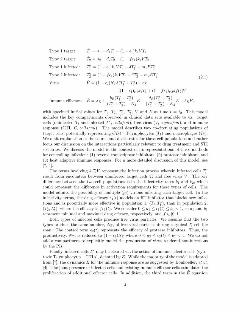
The mathematical model (2.1) contains numerous parameters that must be assignedbefore numerical simulations can be carried out. In specifying model parameters, to thegreatest extent possible we employ values similar to those reported or justified in theliterature. The definitions and numerical values for the parameters are summarized inTable 2, which are principally extracted from the Callaway-Perelson [7] and Bonhoeffer,et al. [4] papers.
parameter value units descriptionλ1 10,000 cells
mL·day target cell type 1 production (source) rated1 0.01∗∗ 1
day target cell type 1 death rateε1 ∈ [0, 1) – efficacy of reverse transcriptase inhibitorε2 ∈ [0, 1) – efficacy of protease inhibitork1 8.0× 10⁻⁷ mL
virions·day population 1 infection rateλ2 31.98 cells
mL·day target cell type 2 production (source) rated2 0.01∗∗ 1
day target cell type 2 death ratef 0.34 (∈ [0, 1]) – treatment efficacy reduction in population 2k2 1× 10⁻⁴ mL
virions·day population 2 infection rateδ 0.7∗ 1
day infected cell death ratem1 1.0× 10⁻⁵ mL
cells·day immune-induced clearance rate for population 1m2 1.0× 10⁻⁵ mL
cells·day immune-induced clearance rate for population 2NT 100∗ virions
cell virions produced per infected cellc 13∗ 1
day virus natural death rateρ1 1 virions
cell average number virions infecting a type 1 cellρ2 1 virions
cell average number virions infecting a type 2 cellλE 1 cells
mL·day immune effector production (source) ratebE 0.3 1
day maximum birth rate for immune effectorsKb 100 cells
mL saturation constant for immune effector birthdE 0.25 1
day maximum death rate for immune effectorsKd 500 cells
mL saturation constant for immune effector deathδE 0.1∗ 1
day natural death rate for immune effectors
Table 1: Parameters used in model (2.1). Those in the top section of the table are takendirectly from Callaway and Perelson. Parameters in the bottom section of the tableare adapted from those in Bonhoeffer, et al.. The superscripts ∗ denote parameters theauthors indicated were estimated from human data and ∗∗ denote those estimated frommacaque data.
Our model choice is in part motivated by its admission of multiple stable steadystates or equilibrium points. This qualitative feature enables us to more accurately
5
model patients such as the “Berlin Patient” [18], who interrupted treatment twice andthen controlled viral infection without further need for drugs, or some of those referencedby the extensive STI literature summary offered by Bajaria, et al. [3], which points toexamples in which some patients have developed immune responses sufficient to controlinfection whereas in others the virus rebounded and again decimated the immune system.For example, in a study of HAART discontinuation [22], three of six patients success-fully suppressed plasma virus for four to more than twenty-four months after stoppingtreatment. These patients exhibited comprehensive and strong HIV-specific immune re-sponses, which are believed responsible for containment of the infection. Other patientsfailed to contain virus at all. Rosenberg, et al. reported on eight subjects in an inter-ruption study [23]. Five of the eight subjects remained off therapy, maintaining viralload less than 500 copies/mL for five to nine months. These subjects exhibited increasedCTL and T-helper cell responses. When studying the STI scenario, it is crucial that themathematical model for HIV infection used be able to represent these different outcomes.
Other authors have considered similar mathematical models with the use of STIto transfer the system between locally stable equilibria or steady states representing“unhealthy” (high viral setpoint, small immune responses) versus “healthy” endpointsfor the patient. Bonhoeffer, et al. [4] explore a model including uninfected targetcells, actively and latently infected target cells, and immune response. They providequalitative analysis including conditions on the model equilibria that will produce each ofthe two possible outcomes. Wodarz and Nowak [26] analyze a model with compartmentsfor uninfected and infected T cells and cytotoxic T lymphocyte precursors (memory) andeffector immune cells. They include analytic expressions for the possible model steadystates as well as analytic conditions on the model parameters that indicate which of theequilibria will be stable.
A general analytical analysis of our model (2.1)’s steady states and their local stabilityis challenging due to the form and number of the nonlinearities. However we are stillinterested in the ability of the model to exhibit multiple locally asymptotically stablesteady states, so we calculate the steady states and perform a standard linearization andeigenvalue analysis of the model, given the numerical values of the parameters specifiedabove.
Letting x = (T1, T2, T∗1 , T ∗2 , V, E) denote the vector of model states, we may represent
the model (2.1) asdx(t)
dt= f(t, x; q), (2.2)
where f(t, x; q) is the right side of the ODE system and q is the vector of model param-eters listed in Table 1. Given the parameter values in Table 1, we invoke Maple to solvef(t, x; q) = 0 for the steady states (equilibria) xk. We next calculate the jacobian matrix(matrix of partial derivatives of the right sides of the differential equations with respectto the state variables):
∂f(t, x; q)∂x
=[∂fi(t, x; q)
∂xj
]
of the ODE system. We set ε1 = ε2 = 0, since we are interested in stability for the
6

off-treatment steady state values. The jacobian matrix is:
−d1 − k1V 0 0 0 −k1T1 00 −d2 − k2V 0 0 −k2T2 0
k1V 0 −δ −m1E 0 k1T1 −m1T∗1
0 k2V 0 −δ −m2E k2T2 −m2T∗2
−ρ1k1V −ρ2k2V NT δ NT δ −c− ρ1k1T1 − ρ2k2T2 00 0 A6,3 A6,4 0 A6,6
,
where
A6,3 = A6,4 =bEKbE
(T ∗1 + T ∗2 + Kb)2 −
dEKdE
(T ∗1 + T ∗2 + Kd)2 ,
and
A6,6 =(
bE
T ∗1 + T ∗2 + Kb− dE
T ∗1 + T ∗2 + Kd
)(T ∗1 + T ∗2 )− δE .
Substituting a computed steady state xk for x in this jacobian matrix, we obtain the ODEsystem dynamics linearized about the equilibrium xk. Linear ODE theory guaranteesthat if the eigenvalues of this matrix all have negative real parts, the equilibrium xk islocally asymptotically stable.
Given the specified parameters, the model (2.1) exhibits three physical steady statesand several non-physical steady states (omitted here) where one or more state variablesare negative. There is a locally unstable equilibrium
T1 = 1000000, T2 = 3198, T ∗1 = 0, T ∗2 = 0, V = 0, E = 10,
which represents an uninfected patient, as well as two locally stable equilibria for aninfected patient in the absence of treatment. These stable steady states are:
“unhealthy”: T1 = 163573, T2 = 5, T ∗1 = 11945, T ∗2 = 46, V = 63919, E = 24;
“healthy”: T1 = 967839, T2 = 621, T ∗1 = 76, T ∗2 = 6, V = 415, E = 353108.
Here the “unhealthy” steady state corresponds to a dangerously high viral set point,depleted T-cells, and minimal immune response, whereas the “healthy” steady staterepresents immune control of the viral infection and restoration of T-cell help. Ourcurrent work includes consideration of optimal strategies for effecting a transfer betweenthese steady states.
The existence and local stability of these equilibria (and indeed the size of theirdomains of attraction) of course depend on the values of the parameters chosen. Acrossa population, the parameter values will vary to represent different host factors andhost-virus interaction rates. For example, the infectivity rates k1 and k2 are crucialdeterminants of the viral load set point. If they are reduced to 10% of their values in thetable, the only stable equilibria are those corresponding to the uninfected scenario (i.e.,clearance of the virus) and one nonphysical steady state. If host immune responsivenessto infection is increased only by setting bE = 0.4, the lone stable steady state is
T1 = 983080, T2 = 1015, T1s = 38, T2s = 5, V = 215, E = 377553,
7
and the immune system controls the persistent viral infection without further treatment.Lori, et al. [19] describe variation across patients in length of time until and strength ofviral rebound when studying patients with STI. The dependence of the model behavioron crucial parameters and their subsequent estimation for individuals may help us predictnot only these variations and those in the studies cited above, but also the expectedresponses to a specific treatment protocol.
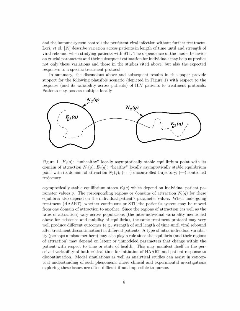
In summary, the discussions above and subsequent results in this paper providesupport for the following plausible scenario (depicted in Figure 1) with respect to theresponse (and its variability across patients) of HIV patients to treatment protocols.Patients may possess multiple locally
N (q)2
������E (q)2
��������������������
��������������������
N (q)1
������E (q)1
���������
���������
Figure 1: E1(q): “unhealthy” locally asymptotically stable equilibrium point with itsdomain of attraction N1(q); E2(q): “healthy” locally asymptotically stable equilibriumpoint with its domain of attraction N2(q); (- - -) uncontrolled trajectory; (—) controlledtrajectory.
asymptotically stable equilibrium states Ei(q) which depend on individual patient pa-rameter values q. The corresponding regions or domains of attraction Ni(q) for theseequilibria also depend on the individual patient’s parameter values. When undergoingtreatment (HAART), whether continuous or STI, the patient’s system may be movedfrom one domain of attraction to another. Since the regions of attraction (as well as therates of attraction) vary across populations (the inter-individual variability mentionedabove for existence and stability of equilibria), the same treatment protocol may verywell produce different outcomes (e.g., strength of and length of time until viral reboundafter treatment discontinuation) in different patients. A type of intra-individual variabil-ity (perhaps a misnomer here) may also play a role since the equilibria (and their regionsof attraction) may depend on latent or unmodeled parameters that change within thepatient with respect to time or state of health. This may manifest itself in the per-ceived variability of both critical time for initiation of HAART and patient response todiscontinuation. Model simulations as well as analytical studies can assist in concep-tual understanding of such phenomena where clinical and experimental investigationsexploring these issues are often difficult if not impossible to pursue.
8
3 Control Formulation
Together with the mathematical model described by equation (2.1) for HIV dynamics,we consider a control problem with the objective function given by
J(ε1, ε2) =∫ t1
t0
[QV (t) + R1ε21 + R2ε
22 − SE(t)] dt, (3.1)
where ε1 and ε2 are the control variables representing RTIs and PIs, respectively. Theparameters Q, R1, R2 and S are weight constants for the virus, controls inputs, andimmune effectors, respectively. The second and third terms in (3.1) represent systemiccosts of the drug treatments (i.e., severity of unintended side effects as well as treatmentcost). The case when ε1(t) = b1 represents maximal use of RT inhibitors and ε2(t) = b2
represents maximal use of protease inhibitors. The objective function (3.1) expresses ourgoal to minimize both the HIV population and systemic costs to body while maximizingimmune response. Therefore, we seek an optimal control pair (ε∗1, ε
∗2) such that
J(ε∗1, ε∗2) = min{J(ε1, ε2)|(ε1, ε2) ∈ U}
subject to the system of ODEs (2.1) and where U = {(ε1, ε2)| εi is measurable, ai ≤ εi ≤bi, t ∈ [t0, t1], for i = 1, 2} is the control set.
A number of researchers have used a control theoretic approach to formulate andstudy dynamic drug therapies for HIV-infected individuals. However, these investiga-tors based their studies on other types of mathematical models for HIV dynamics and/ordifferent objective functionals. For example, the studies in [6, 8, 14] for optimal control ofthe chemotherapy of HIV used an objective function based on a combination of maximiz-ing CD4+ T cell counts while minimizing the systemic cost of chemotherapy. H.R. Joshi[11] considered two different treatment strategies (controls) in a mathematical modelconsisting of only two states: uninfected CD4+ T cells and viral loads. His controlsrepresent immune boosting and viral suppressing drugs. Another deterministic controlproblem, proposed by Wein et al. [25], is based on a finite number of virus strains andallows mutations from one strain to another. Due to the high dimensionality of the con-trol problem, the authors resort to an approximate method, which employs perturbationmethods in conjunction with ideas from dynamic programming to derive a closed formdynamic therapeutic policy. Using numerical simulations, they demonstrated a dynamicstrategy that reduces the total free virus, increases the uninfected CD4+ count, and de-lays the emergence of drug-resistant strains. A similar study by J.J. Kutch and P. Gurfil[16] involves optimal control of HIV infection to derive an optimal drug administrationscheme that may be useful in increasing patient health by delaying the emergence ofdrug-resistant mutant viral strains. Feedback control in HIV-1 populations is exploredin [5]. There the authors considered several methods of stable control of the HIV pop-ulation using an external feedback control term that is analogous to the introduction ofa therapeutic drug regimen. The feedback control, based on periodic sampling of viralload and lymphocyte counts, uses a target tracking approach. Using this regimen designthey showed that once the virus is controlled to very low levels the drug dosage can be
9
reduced proportionately. Under such circumstances it is suggested that side effects oftherapy will also be mitigated.
Here we use an open loop control formulation to treat both continuous and STIcontrol of the system (2.1) with the cost functional (3.1).
3.1 The Optimality System
We begin this section by noting that the existence of an optimal control pair can beobtained using a result from Fleming and Rishel [9]. That is, it is rather straightforwardto show that the right sides of the equation (2.1) are bounded by a linear function ofthe state and control variables and that the integrand of the objective function (3.1) isconcave on U and is bounded below. These bounds give one the compactness needed toestablish existence of the optimal controls using standard arguments given in [9].
We now proceed to compute candidates for optimal controls. To this end, we applythe Pontryagin Minimum Principle and begin by defining the Lagrangian (which is theHamiltonian augmented with penalty terms for the constraints) to be:
L(T1, T2, T∗1 , T ∗2 , V, E, ε1, ε2, ξ1, ξ2, ξ3, ξ4, ξ5, ξ6)
= QV + R1ε21 + R2ε
22 − SE + ξ1
(λ1 − d1T1 − (1− ε1)k1V T1
)
+ξ2
(λ2 − d2T2 − (1− fε1)k2V T2
)
+ξ3
((1− ε1)k1V T1 − δT ∗1 −m1ET ∗1
)
+ξ4
((1− fε1)k2V T2 − δT ∗2 −m2ET ∗2
)
+ξ5
((1− ε2)NT δ(T ∗1 + T ∗2 )− cV
−[(1− ε1)ρ1k1T1 + (1− fε1)ρ2k2T2]V)
+ξ6
(λE +
bE(T ∗1 + T ∗2 )(T ∗1 + T ∗2 ) + Kb
E − dE(T ∗1 + T ∗2 )(T ∗1 + T ∗2 ) + Kd
E − δEE)
−w11(ε1 − a1)− w12(b1 − ε1)−w21(ε2 − a2)− w22(b2 − ε2),
(3.2)
where wij(t) ≥ 0 are the penalty multipliers satisfying
w11(t)(ε1(t)− a1) = w12(t)(b1 − ε1(t)) = 0 at ε1 = ε∗1
andw21(t)(ε2(t)− a2) = w22(t)(b2 − ε2(t)) = 0 at ε2 = ε∗2.
Here (ε∗1, ε∗2) is the optimal control pair yet to be found. Differentiating the Lagrangian
with respect to state variables, T1, T2, T ∗1 , T ∗2 , V, and E, respectively, we obtain thefollowing equations for the adjoint variables ξi :
ξ1 = − ∂L
∂T1, ξ2 = − ∂L
∂T2, ξ3 = − ∂L
∂T ∗1, ξ4 = − ∂L
∂T ∗2, ξ5 = − ∂L
∂Vand ξ6 = − ∂L
∂E.
10
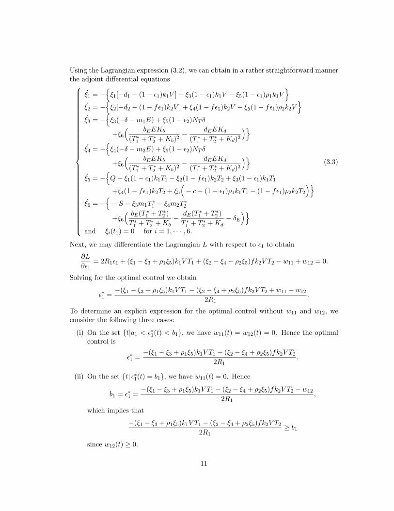
Using the Lagrangian expression (3.2), we can obtain in a rather straightforward mannerthe adjoint differential equations
ξ1 = −{
ξ1[−d1 − (1− ε1)k1V ] + ξ3(1− ε1)k1V − ξ5(1− ε1)ρ1k1V}
ξ2 = −{
ξ2[−d2 − (1− fε1)k2V ] + ξ4(1− fε1)k2V − ξ5(1− fε1)ρ2k2V}
ξ3 = −{
ξ3(−δ −m1E) + ξ5(1− ε2)NT δ
+ξ6
( bEEKb
(T ∗1 + T ∗2 + Kb)2− dEEKd
(T ∗1 + T ∗2 + Kd)2)}
ξ4 = −{
ξ4(−δ −m2E) + ξ5(1− ε2)NT δ
+ξ6
( bEEKb
(T ∗1 + T ∗2 + Kb)2− dEEKd
(T ∗1 + T ∗2 + Kd)2)}
ξ5 = −{
Q− ξ1(1− ε1)k1T1 − ξ2(1− fε1)k2T2 + ξ3(1− ε1)k1T1
+ξ4(1− fε1)k2T2 + ξ5
(− c− (1− ε1)ρ1k1T1 − (1− fε1)ρ2k2T2
)}
ξ6 = −{− S − ξ3m1T
∗1 − ξ4m2T
∗2
+ξ6
( bE(T ∗1 + T ∗2 )T ∗1 + T ∗2 + Kb
− dE(T ∗1 + T ∗2 )T ∗1 + T ∗2 + Kd
− δE
)}
and ξi(t1) = 0 for i = 1, · · · , 6.
(3.3)
Next, we may differentiate the Lagrangian L with respect to ε1 to obtain
∂L
∂ε1= 2R1ε1 + (ξ1 − ξ3 + ρ1ξ5)k1V T1 + (ξ2 − ξ4 + ρ2ξ5)fk2V T2 − w11 + w12 = 0.
Solving for the optimal control we obtain
ε∗1 =−(ξ1 − ξ3 + ρ1ξ5)k1V T1 − (ξ2 − ξ4 + ρ2ξ5)fk2V T2 + w11 − w12
2R1.
To determine an explicit expression for the optimal control without w11 and w12, weconsider the following three cases:
(i) On the set {t|a1 < ε∗1(t) < b1}, we have w11(t) = w12(t) = 0. Hence the optimalcontrol is
ε∗1 =−(ξ1 − ξ3 + ρ1ξ5)k1V T1 − (ξ2 − ξ4 + ρ2ξ5)fk2V T2
2R1.
(ii) On the set {t| ε∗1(t) = b1}, we have w11(t) = 0. Hence
b1 = ε∗1 =−(ξ1 − ξ3 + ρ1ξ5)k1V T1 − (ξ2 − ξ4 + ρ2ξ5)fk2V T2 − w12
2R1,
which implies that
−(ξ1 − ξ3 + ρ1ξ5)k1V T1 − (ξ2 − ξ4 + ρ2ξ5)fk2V T2
2R1≥ b1
since w12(t) ≥ 0.
11

(iii) On the set {t| ε∗1(t) = a1}, we have w12(t) = 0. Hence
a1 = ε∗1 =−(ξ1 − ξ3 + ρ1ξ5)k1V T1 − (ξ2 − ξ4 + ρ2ξ5)fk2V T2 + w11
2R1,
which implies that
−(ξ1 − ξ3 + ρ1ξ5)k1V T1 − (ξ2 − ξ4 + ρ2ξ5)fk2V T2
2R1≤ a1
since w11(t) ≥ 0.
Combining these three cases, the optimal control ε1 is characterized as
ε∗1 = max(a1, min
(b1,
−(ξ1 − ξ3 + ρ1ξ5)k1V T1 − (ξ2 − ξ4 + ρ2ξ5)fk2V T2
2R1
)). (3.4)
Using similar arguments, we also obtain the following expression for the second optimalcontrol function
ε∗2 = max(a2, min
(b2,
ξ5NT δ(T ∗1 + T ∗2 )2R2
)). (3.5)
The optimality system consists of the state system (2.1) coupled with the adjointsystem (3.3) with the initial conditions and terminal conditions together with the ex-pressions (3.4) and (3.5) for the control functions.
4 Numerical Results: Continuous Optimal Therapy
We point out that (as is standard in such formulations) initial conditions are specified forthe state system (2.1), whereas terminal conditions are specified for the adjoint system(3.3). Therefore the optimality system is a two-point boundary value problem, which wesolve numerically using a gradient method. The state system with initial conditions issolved forward in time using initial guesses for the controls and then the adjoint systemwith terminal conditions is solved backward in time. The controls are updated in eachiteration using the formulas (3.4) and (3.5) for optimal controls. The iterations continueuntil convergence is achieved. For further discussion of this iterative method we referthe interested reader to [10]. The parameters used in solving the optimality system arethose summarized in Table 1. Treatment was simulated for 400 days.
We simulate early infection by perturbing the “uninfected” unstable steady state, in-troducing one virus particle per ml of blood plasma and very low levels of infected T-cells.That is, we take initial conditions T1(0) = 106, T2(0) = 3198, T ∗1 (0) = 10−4, T ∗2 (0) =10−4, V (0) = 1 and E(0) = 10. We bound drug efficacies by a1 = 0, a2 = 0, b1 = 0.7and b2 = 0.3. Since the magnitudes of the virus population, drug treatment functions,and immune effector population in the objective function (3.1) are on different scales,we balance them by choosing weighting values Q = 0.1, R1 = 20000, R2 = 20000, andS = 1000.
12

0 50 100 150 200 250 300 350 4000
0.1
0.2
0.3
0.4
0.5
0.6
0.7
days
epsi
lon_
1
0 50 100 150 200 250 300 350 4000
0.05
0.1
0.15
0.2
0.25
0.3
days
epsi
lon_
2
Figure 2: Optimal control pair with Q = 0.1, R1 = 20000, R2 = 20000 and S = 1000.The label ε1 represents RT inhibitors and ε2 represents protease inhibitors.
The optimal control function pair is depicted in Figure 2. We then determine the sys-tem behavior under this regimen by simulating the state equations (2.1). These optimalsolutions together with non-optimal solutions corresponding to no drug treatments (i.e.,ε1 = ε2 ≡ 0) and with fully efficacious persistent treatment using both RT inhibitors andprotease inhibitors (i.e., ε1 ≡ 0.7 and ε2 ≡ 0.3) are presented in Figure 3 for comparison.
As depicted in Figure 2 the shapes of the two control functions are nearly identical.Perhaps the most intriguing observation from this figure is the STI-like characteristicsof the optimal dynamic therapies. In particular, both drugs are tapered off around the30th, 100th, 200th and 300th days. Consequently, the virus (V ) and infected target cells(T ∗1 and T ∗2 ) counts are relatively high around those days (Figure 3). This high virusload, in turn, stimulates the immune effectors (E) in order to boost immune responses.
From Figure 3, we observe that the population of uninfected T1 cells correspondingto the optimal control pair approaches the population of uninfected T1 cells with fulltreatment of both drugs at the end of the time period. Moreover, the virus load withthe optimal control pair is maintained at low levels except at the 100th, 200th and 300th
13

0 100 200 300 4004
4.5
5
5.5
6
days
log(
T1
cells
)
0 100 200 300 400−1
0
1
2
3
4
days
log(
T2
cells
)
0 100 200 300 400−5
0
5
days
log(
T1*
cel
ls)
0 100 200 300 400−4
−2
0
2
4
days
log(
T2*
cel
ls)
0 100 200 300 400−2
0
2
4
6
days
log(
Viru
s)
0 100 200 300 4000
2
4
6
days
log(
E)
Figure 3: Optimal solutions (−); solutions (−−) with fully efficacious treatment of bothdrugs (i.e., ε1 ≡ 0.7 and ε2 ≡ 0.3); and solutions (−·) with no treatments of both drugs(i.e., ε1 = ε2 ≡ 0) of early infection: Q = 0.1, R1 = 20000, R2 = 20000 and S = 1000.
days and is even smaller at the 400th day due to the high immune effectors (E). Thishappens even though both optimal control functions are very close to zero at the 400th
day.Indeed, our initial numerical results are very promising. They show the potential
to design optimal therapeutic options that minimize the total viral load, increase theuninfected CD4+-T cell counts, and boost immune response while allowing patientsvery brief drug holidays. However, optimal continuous therapy is not practical sincein a clinical setting treatment can only be altered at intervals. In the next section,we derive optimal HIV therapeutic strategies that provide clinical benefits similar tothose of the continuous treatment while allowing for supervised, or structured, treatmentinterruption.
14

5 Optimal STI Therapies
In this section we consider optimal control of viral load through drug structured treat-ment interruptions (STIs). More precisely, we consider optimal STI control in order todetermine the best schedules in which patients are put on and off therapy over predefinedperiods of time.
Here we assume the (time discretized) controls ε1 and ε2 have vector forms (i.e., arediscrete resulting from being either on or off each day) and consist of only 0 or bi in eachcomponent. If a component of a control vector is 0, it indicates drug treatment is off onthat day and if it is bi, it indicates full drug treatment is on. Since we consider a drugtreatment strategy over 900 days, the size of each control vector is 1× 900. The set ofall such control vectors is denoted by Λ. The goal is to seek the optimal control vectorpair (ε∗1,ε
∗2) satisfying
minε1,ε2∈Λ
J(ε1, ε2) = J(ε∗1, ε∗2)
subject to the state system (2.1) and where J(ε1, ε2) is defined by (3.1).Since the number of elements of the set Λ is finite, the existence of an optimal control
vector pair is guaranteed. We could use a crude direct search approach [1] involvingsimple comparisons to find the optimal STI control pair. That is, we could begin byselecting any pair from the set Λ and then solving the state system using this pair ascontrols. We would next select another pair from the set Λ and again solve the statesystem using the pair as controls. Upon comparing the values of objective functional, J ,we select the control pair corresponding to the smaller cost functional value. If we iteratethis strategy over all possible pairs from the set Λ, we obtain the optimal control vectorpair, ε∗1 and ε∗2. However, this strategy to obtain the optimal STI control pair leadsto a large number of cost functional evaluations and hence a large number of solutionsto the state system (2.1). In our example, the number of cost functional evaluationswould be (2900)2 since each control vector is a 1× 900 vector. This makes this approachcomputationally infeasible.
We therefore seek to reduce the number of iterations, and consider several ideas toaccomplish this goal. One is to consider 5 day segments instead of 1 day segments asabove. This is more reasonable from a practical point of view since it is not clinicallyfeasible for drug strategies to allow change with a daily frequency. For 5 day segments,the size of each control vector is reduced to 1× 180 from 1× 900. However the reducednumber of iterations is (2180)2 which is still quite large.
One approach to further alleviate this computational burden is to consider subperiodsof the given period such as [0, 30], [0, 60], [0, 90], [0, 120], · · · , [0, 900]. This approach,which is similar to the underlying idea for dynamic programming, is discussed and usedin [1] where only single drug therapies are considered. We shall refer to this simply as the“subperiod method”. In this method, we find an optimal STI control pair, (ε∗1,1, ε∗1,2),over the first subperiod, [0, 30], using the reduced iteration technique (5 day segments)as above. Since the size of ε∗1,1 and ε∗1,2 is 1×6 (for 5 day segments over 30 days), optimalsolutions can be obtained very quickly (with only (26)2 = 4096 iterations). In the second
15

step, we consider our control vectors over the period [0, 60] as follows:
ε2,1 = [ε∗1,1, ?, ?, ?, ?, ?, ?] and ε2,2 = [ε∗1,2, ?, ?, ?, ?, ?, ?]
where ? is 0 or bi. That is, we fix the [0, 30] optimal STI pair, ε∗1,1 and ε∗1,2 , as the first6 elements of the controls, ε2,1 and ε2,2, respectively, and iterate ε2,1 and ε2,2 to find thelast 6 elements of each control that make an “optimal” STI control pair, (ε∗2,1, ε∗2,2), overthe period [0, 60]. In this case, the number of iterations is also just (26)2 = 4096 so wecan obtain it quickly. We repeat this process to find an “optimal” STI control pair, (ε∗3,1,ε∗3,2), over [0, 90], (ε∗4,1, ε∗4,2), over [0, 120], and so on. The STI control pair obtainedover the whole period [0, 900] is ε∗1 = ε∗30,1 and ε∗2 = ε∗30,2. It should be emphasized thatthe STI control pair, ε∗1 and ε∗2 is now only suboptimal. However, we observed in [1],where only single drug therapies were considered, that this subperiod approach yieldeda suboptimal STI therapy that produces results which are reasonable approximations tothose for a fully efficacious continuous therapy as well as to those for an optimal STItherapy in some examples.
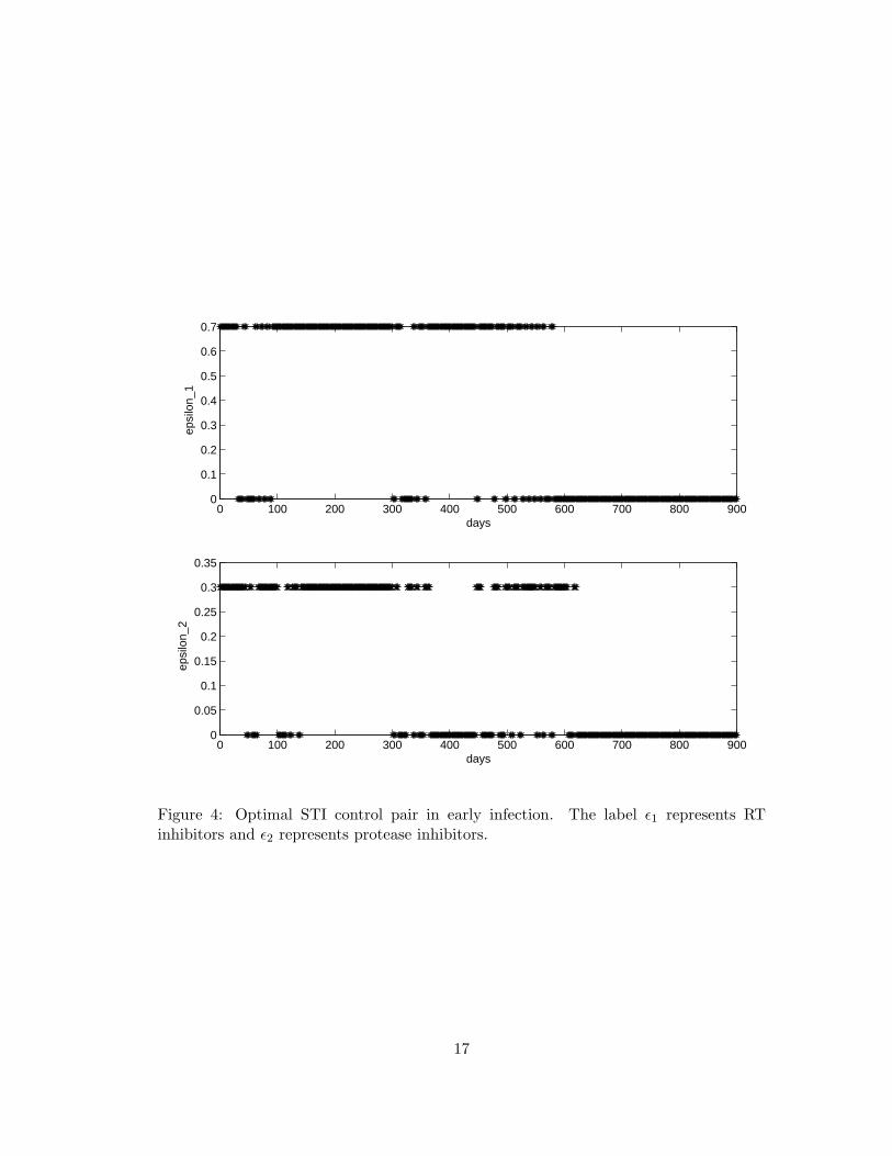
We again simulate early infection by introducing one virus particle per ml of bloodplasma, i.e., T1(0) = 106, T2(0) = 3198, T ∗1 (0) = 10−4, T ∗2 (0) = 10−4, V (0) = 1 andE(0) = 10. And we also use a1 = 0, a2 = 0, b1 = 0.7 and b2 = 0.3. Using the subperiodmethod, a suboptimal STI control pair and associated solutions are depicted in Figure4 and Figure 5, respectively. We note that PI therapy is interrupted more than RTinhibitors, especially between the 300th day and the 500th day. Notable features includethat the virus load remains less than 103 and the population of uninfected T1 cellsrecovers from the effects of HIV after around the 600th day even though both drugs arediscontinued at that time. This is due to a very strong immune response. We noticethat both drugs are interrupted around the 50th and 300th days. These interruptionscause extremely high virus load in turn leads to more infected T ∗1 and T ∗2 cells at thosetimes. Immune response is thus stimulated and augmented especially through theseinterruptions. This is a good example of moving a patient from an infected state to ahealthy state.
16
0 100 200 300 400 500 600 700 800 9000
0.1
0.2
0.3
0.4
0.5
0.6
0.7
days
epsi
lon_
1
0 100 200 300 400 500 600 700 800 9000
0.05
0.1
0.15
0.2
0.25
0.3
0.35
days
epsi
lon_
2
Figure 4: Optimal STI control pair in early infection. The label ε1 represents RTinhibitors and ε2 represents protease inhibitors.
17

0 200 400 600 8004
4.5
5
5.5
6
days
log(
T1
cells
)
0 200 400 600 800−1
0
1
2
3
4
days
log(
T2
cells
)
0 200 400 600 800−5
0
5
days
log(
T1*
cel
ls)
0 200 400 600 800−4
−2
0
2
4
days
log(
T2*
cel
ls)
0 200 400 600 800−2
0
2
4
6
days
log(
Viru
s)
0 200 400 600 8001
2
3
4
5
6
days
log(
E)
Figure 5: STI control solutions (−), solutions (−·) with no treatments of both drugs(ε1 = ε2 ≡ 0), solutions (−−) with fully efficacious treatment of both drugs (ε1 ≡ 0.7 andε2 ≡ 0.3) in early infection over the period [0, 900]. Q = 0.1, R1 = 20000, R2 = 20000and S = 1000.
18
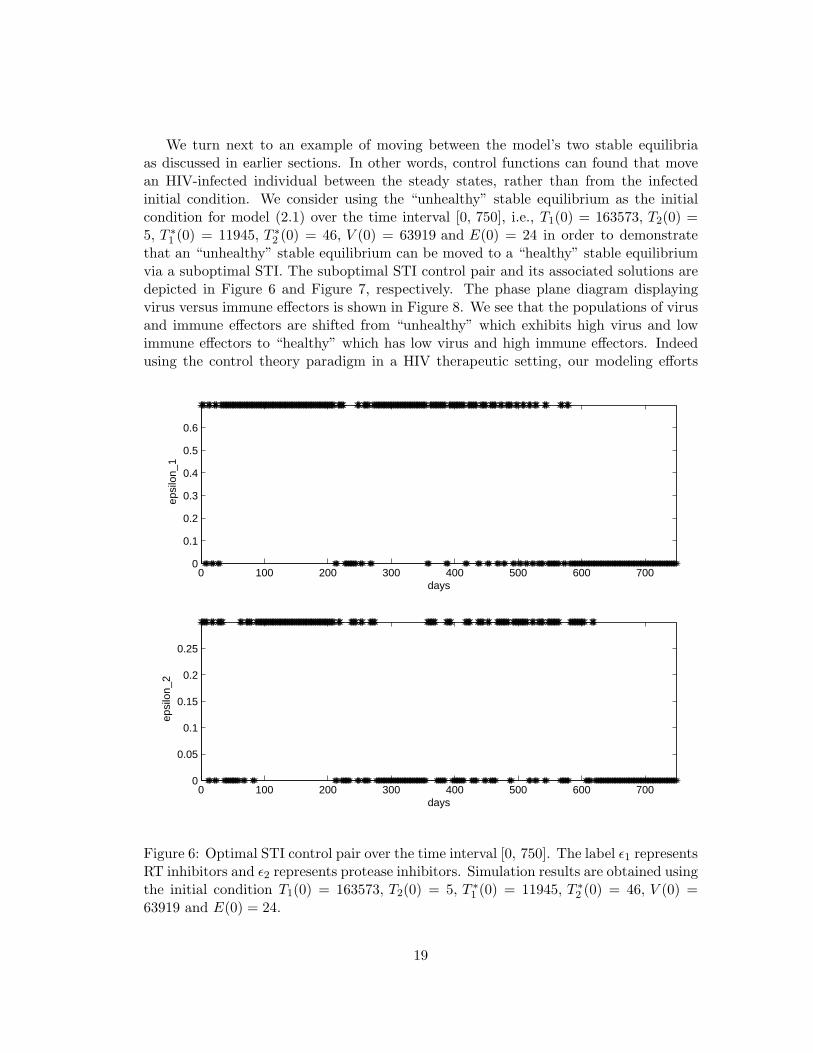
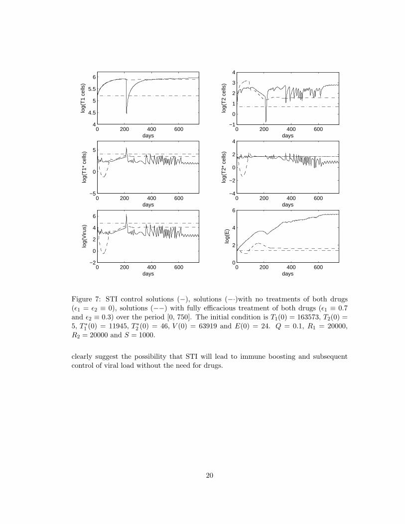
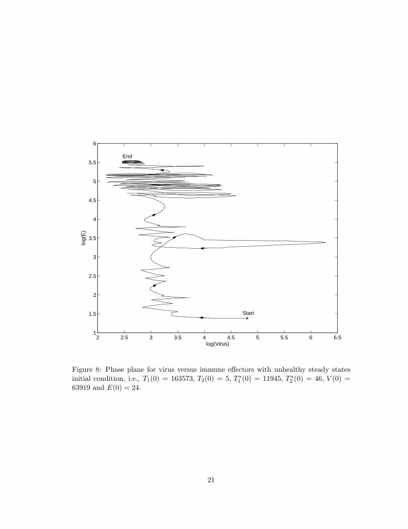
We turn next to an example of moving between the model’s two stable equilibriaas discussed in earlier sections. In other words, control functions can found that movean HIV-infected individual between the steady states, rather than from the infectedinitial condition. We consider using the “unhealthy” stable equilibrium as the initialcondition for model (2.1) over the time interval [0, 750], i.e., T1(0) = 163573, T2(0) =5, T ∗1 (0) = 11945, T ∗2 (0) = 46, V (0) = 63919 and E(0) = 24 in order to demonstratethat an “unhealthy” stable equilibrium can be moved to a “healthy” stable equilibriumvia a suboptimal STI. The suboptimal STI control pair and its associated solutions aredepicted in Figure 6 and Figure 7, respectively. The phase plane diagram displayingvirus versus immune effectors is shown in Figure 8. We see that the populations of virusand immune effectors are shifted from “unhealthy” which exhibits high virus and lowimmune effectors to “healthy” which has low virus and high immune effectors. Indeedusing the control theory paradigm in a HIV therapeutic setting, our modeling efforts
0 100 200 300 400 500 600 7000
0.1
0.2
0.3
0.4
0.5
0.6
days
epsi
lon_
1
0 100 200 300 400 500 600 7000
0.05
0.1
0.15
0.2
0.25
days
epsi
lon_
2
Figure 6: Optimal STI control pair over the time interval [0, 750]. The label ε1 representsRT inhibitors and ε2 represents protease inhibitors. Simulation results are obtained usingthe initial condition T1(0) = 163573, T2(0) = 5, T ∗1 (0) = 11945, T ∗2 (0) = 46, V (0) =63919 and E(0) = 24.
19
0 200 400 6004
4.5
5
5.5
6
days
log(
T1
cells
)
0 200 400 600−1
0
1
2
3
4
days
log(
T2
cells
)
0 200 400 600−5
0
5
days
log(
T1*
cel
ls)
0 200 400 600−4
−2
0
2
4
days
log(
T2*
cel
ls)
0 200 400 600−2
0
2
4
6
days
log(
Viru
s)
0 200 400 6000
2
4
6
days
log(
E)
Figure 7: STI control solutions (−), solutions (−·)with no treatments of both drugs(ε1 = ε2 ≡ 0), solutions (−−) with fully efficacious treatment of both drugs (ε1 ≡ 0.7and ε2 ≡ 0.3) over the period [0, 750]. The initial condition is T1(0) = 163573, T2(0) =5, T ∗1 (0) = 11945, T ∗2 (0) = 46, V (0) = 63919 and E(0) = 24. Q = 0.1, R1 = 20000,R2 = 20000 and S = 1000.
clearly suggest the possibility that STI will lead to immune boosting and subsequentcontrol of viral load without the need for drugs.
20
2 2.5 3 3.5 4 4.5 5 5.5 6 6.51
1.5
2
2.5
3
3.5
4
4.5
5
5.5
6
log(Virus)
log(
E)
Start
End
Figure 8: Phase plane for virus versus immune effectors with unhealthy steady statesinitial condition, i.e., T1(0) = 163573, T2(0) = 5, T ∗1 (0) = 11945, T ∗2 (0) = 46, V (0) =63919 and E(0) = 24.
21

6 Concluding Remarks
In this paper we have formulated a dynamic model with compartments including targetcells, infected cells, virus, and immune response that is subject to multiple (RTI- andPI-like) drug treatments as control inputs. For certain ranges of the parameters, the un-controlled model possesses multiple locally asymptotically stable steady states. We thenapplied techniques and ideas from open loop control theory and dynamic programmingto derive continuous and suboptimal STI therapy protocols. In particular, we use the“subperiod method” introduced in [1] for therapies involving a single drug to developresults for drug “cocktails”. We demonstrate that one can use the resulting suboptimalSTI strategies to move the model system from an “unhealthy” locally stable region ofattraction to a similar “healthy” one in which the immune response is dominant in con-trolling the viral levels. This illustrates one possible scenario by which STI therapiescould lead to long term control of HIV after discontinuation of therapy.
Acknowledgments
This research was supported in part by the Joint DMS/NIGMS Initiative to SupportResearch in the Area of Mathematical Biology under grant 1R01GM67299-01, and wasfacilitated through visits of the authors to the Statistical and Applied MathematicalSciences Institute, (SAMSI), which is funded by NSF under grant DMS-0112069.
References
[1] B.M. Adams, H.T. Banks, M. Davidian, Hee-Dae Kwon, H.T. Tran, S.N. Wynne,and E.S. Rosenberg, HIV Dynamics: Modeling, data analysis, and optimal treat-ment protocols, CRSC Tech. Rpt. CRSC-TR04-05, NCSU, Raleigh, February, 2004;special issue of J. Comp. Appl. Math. on “Mathematics Applied to Immunology”,submitted.
[2] Z. Agur, A new method for reducing cytotoxicity and the anti-AIDS drug AZT,Biomedical Modeling and Simulation, Editor: D.S. Levine, J.C. Baltzer AG, Scien-tific Publishing Co. IMACS, (1989), 59-61.
[3] S.H. Bajaria, G. Webb, and D.E. Kirschner, Predicting differential responses tostructured treatment interruptions during HAART, Bull. Math. Biol., to appear.
[4] S. Bonhoeffer, M. Rembiszewski, G.M. Ortiz, and D.F. Nixon, Risks and benefits ofstructured antiretroviral drug therapy interruptions in HIV-1 infection, AIDS, 14(2000), 2313-2322.
[5] M.E. Brandt and B Chen, Feedback control of a biodynamical model of HIV-1,IEEE Trans. on Biom. Engr., 48 (2001), 754-759.
22
[6] S. Butler, D. Kirschner and S. Lenhart, Optimal control of the chemotherapy af-fecting the infectivity of HIV, in Advances in Mathematical Population Dynamics-Molecules, Cells and Man, Editors: O. Arino, D. Axelrod and M. Kimmel, WordScientific Press, Singapore, (1997), 557-569.
[7] D. S. Callaway and A. S. Perelson, HIV-1 infection and low steady state viral loads,Bull. Math. Biol., 64 (2001), 29-64.
[8] K.R. Fister, S. Lenhart and J.S. McNally, Optimizing chemotherapy in an HIVmodel, Electr. J. Diff. Eq., 32 (1998), 1-12.
[9] W.H. Fleming and R.W. Rishel, Deterministic and Stochastic Optimal Control,Springer-Verlag, New York, 1975.
[10] M.D. Gunzburger, Perspectives in Flow Control and Optimization, SIAM, Philadel-phia, 2003.
[11] H.R. Joshi, Optimal control of an HIV immunology model, Optim. Contr. Appl.Math, 23 (2002), 199-213.
[12] M.I. Kamien and N.L. Schwartz, Dynamic Optimization, North-Holland, Amster-dam, 1991.
[13] D. Kirschner, S. Lenhart and S. Serbin, A model for treatment strategy in thechemotherapy of aids, Bull. Math. Biol., 58 (1996), 367-390.
[14] D. Kirschner, S. Lenhart and S. Serbin, Optimal control of the chemotherapy ofHIV, J. Math. Biol., 35 (1997), 775-92.
[15] D. Kirschner and G. Webb, A model for treatment strategy in the chemotherapy ofAIDS, Bull. Math. Biol., 58 (1996), 367-390.
[16] J.J. Kutch and P. Gurfil, Optimal control of HIV infection with a continuously-mutating viral population, in Proc. of the American Control Conference, Anchorage,AK, (2002). 4033-4038.
[17] J. Lisziewicz and F. Lori, Structured treatment interruptions in HIV/AIDS therapy,Microbes and Infection, 4 (2002), 207-214.
[18] J. Lisziewicz, E. Rosenberg and J. Liebermann, Control of HIV despite the discon-tinuation of anti-retroviral therapy, New England J. Med., 340 (1999), 1683-1684.
[19] F. Lori, R. Maserati, et al., Structured treatment interruptions to control HIV-1infection, The Lancet, 354 (2000), 287-288.
[20] D.L. Lukes, Differential Equations: Classical to Controlled, Mathematics in Scienceand Engineering, Academic Press, New York, 1982.
23

[21] G.S. Ogg, et al., Quantitation of HIV-1-specific cytotoxic T lymphocytes and plasmaload of viral RNA, Science, 279 (1998), 2103-2106.
[22] G. M. Ortiz, D. F. Nixon, et al., HIV-1-specific immune responses in subjectswho temporariliy contain virus replication after discontinuation of highly activeantiretroviral therapy, J. Clin. Invest., 104 (1999), R13-R18.
[23] E. S. Rosenberg, M. Altfield and S. H. Poon, Immune control of HIV-1 after earlytreatment of acute infection, Nature, 407 (2000), 523-526.
[24] L. Ruiz, et al., Structured treatment interruption in chronically HIV-1 infectedpatients after long-term viral suppression, AIDS, 14 (2000), 397-403.
[25] L.M. Wein, S.A. Zenios and M.A. Nowak, Dynamic multidrug therapies for HIV: Acontrol theoretic approach, J. Theor. Biol., 185 (1997), 15-29.
[26] D. Wodarz and M.A. Nowak, Specific therapy regimes could lead to long-termimmunological control of HIV, Proc. Natl. Acad. Sci., 96 (1999), 14464-14469.
24