Dynamic modeling of electromagnetic suspension system

http://jvc.sagepub.com/Journal of Vibration and Control

http://jvc.sagepub.com/content/early/2012/02/21/1077546312438601The online version of this article can be found at:

DOI: 10.1177/1077546312438601

published online 21 February 2012Journal of Vibration and ControlNam H Kim and Long Ge

Dynamic modeling of electromagnetic suspension system

Published by:

http://www.sagepublications.com

can be found at:Journal of Vibration and ControlAdditional services and information for

http://jvc.sagepub.com/cgi/alertsEmail Alerts:

http://jvc.sagepub.com/subscriptionsSubscriptions:

http://www.sagepub.com/journalsReprints.navReprints:

http://www.sagepub.com/journalsPermissions.navPermissions:

What is This?

- Feb 21, 2012OnlineFirst Version of Record >>

at UNIV OF FLORIDA Smathers Libraries on March 15, 2012jvc.sagepub.comDownloaded from

XML Template (2012) [20.2.2012–5:35pm] [1–13]K:/JVC/JVC 438601.3d (JVC) [PREPRINTER stage]

Article

Dynamic modeling of electromagneticsuspension system

Nam H Kim and Long Ge

Abstract

Characteristics of magnetic-levitation systems are studied using dynamic models that include motion-dependent lift, drag,

slip, and roll motions. The contact constraint between the vehicle and the track is modeled using a compliant contact

model, and inelastic restitution is modeled using damping. Unknown numerical parameters are identified using an

optimization technique and experimental data. The numerical tests are focused on the damping characteristics, stability

in lifting and slip motions, the lifting efficiency, and the contact behavior with the track. It turns out that the suspension

system does not have any inherent damping in the lifting direction. However, a stable behavior is observed in the traveling

direction. The model also shows that the system has a strong concentric force that stabilizes the vehicle in the slip

motion as well as in the rolling motion.

Keywords

Dynamic model, magnetic levitation, suspension, contact, regression

Received: 30 April 2009; accepted: 10 July 2011

1. Introduction

The maglev (magnetic-levitation) system utilizes mag-netic fields produced from ground based electricalpower sources to levitate a vehicle above the track.The vehicle is then accelerated along the track usinghigh-power electromagnets (Powell and Danby, 1971;Luerkin, 1994; Kalsi, 1994; Rote and Cai, 2002).Recently, Post and Ryutov (1996, 2000) proposed anew concept, Inductrack, that provides a passivemeans of levitation. The realization of a stabilizedride using maglev has been a major hurdle in develop-ing its feasibility for this purpose. The main scope ofthis paper is to examine the feasibility of the Inductrackmagnetic-levitation system, developed at the LawrenceLivermore National Laboratory, by identifying thedynamic characteristics of the magnetic-levitation sus-pension system with computational dynamic analysis.

The maglev system is composed of a vehicle (cradle)with permanent magnets and a rail with coils in it. Themagnets and the coils produce an electromagnetic field,and once the cradle starts moving, the change in themagnetic field results in an electromagnetic force.A moving cradle with a special configuration of high-strength permanent magnets generates passive magnetic

levitation when it moves over multi-loops of wireembedded in the track underneath. This system is con-figured so that the resulting electromagnetic forces aredecomposed into driving forces and lifting forces.Compared with other maglev systems, the Inductracksystem can provide levitation forces with simpler andless expensive equipment.

The early stages of development of the maglevsystem have focused on how to generate enough liftingforce using a special array of magnets. It has been dem-onstrated by Post and Ryutov (2000) that theInductrack concept can be used to build a simplerand less expensive system using a Halbach array(Halbach, 1985) of permanent magnets, which inducesrepelling currents in a close-packed array of shortedconducting circuits in the track. Basing their study onlumped-circuit analysis, they showed that the maximum

Department of Mechanical and Aerospace Engineering, University of

Florida, USA

Corresponding author:

Nam H Kim, Department of Mechanical and Aerospace Engineering,

University of Florida, Gainesville, FL 32611, USA

Email: [email protected]

Journal of Vibration and Control

0(0) 1–13

! The Author(s) 2012

Reprints and permissions:

sagepub.co.uk/journalsPermissions.nav

DOI: 10.1177/1077546312438601

jvc.sagepub.com


http://jvc.sagepub.com/


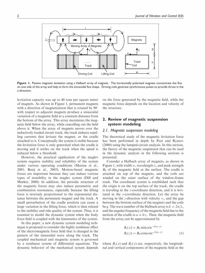
levitation capacity was up to 40 tons per square meterof magnets. As shown in Figure 1, permanent magnetswith a direction of magnetization that is rotated by 90�

with respect to adjacent magnets produce a sinusoidalvariation of a magnetic field at a constant distance fromthe bottom of the array. This array maximizes the mag-netic field below the array, while cancelling out the fieldabove it. When the array of magnets moves over theinductively loaded circuit track, the track induces repel-ling currents that levitate the magnet, or the cradleattached to it. Conceptually the system is stable becausethe levitation force is only generated when the cradle ismoving and it settles on the track when the speed isreduced below a threshold.

However, the practical application of the maglevsystem requires stability and reliability of the systemunder various operating conditions (Matsue et al.,2001; Boeij et al., 2005). Motion-based magneticforces are important because they can induce varioustypes of instability in the maglev system (Dill andMeeker, 2000). In addition, the periodic structure ofthe magnetic forces may also induce parametric andcombination resonances, especially because the liftingforce is inversely proportional to the exponential dis-tance between the permanent magnet and the track. Asmall perturbation of the cradle position can cause alarge variation in the lifting force, which is then relatedto the stability and ride quality of the system. Thus, it isessential to model the dynamic system when the bodyforce field is coupled with the kinematics of the system.

In this paper, a new dynamic system modeling tech-nique is proposed to consider the highly nonlinear effectof the electromagnetic force field that is changed in thepattern of the sinusoidal wave along the track. Thecoupled mechanical and magnetic system is governedby a nonlinear system of differential equations. Thedynamic behavior of the mechanical system depends

on the force generated by the magnetic field, while themagnetic force depends on the location and velocity ofthe structure.

2. Review of magnetic suspensionsystem modeling

2.1. Magnetic suspension modeling

The theoretical study of the magnetic levitation forcehas been performed in depth by Post and Ryutov(2000) using the lumped-circuit analysis. In this section,the theory of the magnetic suspension that can be usedin the dynamic analysis in the following sections ispresented.

Consider a Halbach array of magnets, as shown inFigure 1, with width w, wavelength �, and peak strengthB0 of the magnetic field at the surface. The cradle isattached on top of the magnets, and the coils arewinded on the outer surface of the window-frametrack. The coordinate system is established such thatthe origin is on the top surface of the track, the cradleis traveling in the z-coordinate direction, and it is levi-tated in the y-coordinate direction. Let the array bemoving in the z-direction with velocity vz, and the gapbetween the bottom surface of the magnets and the coilsbe g. Thewave number of theHalbach array is k ¼ 2�=�,and the angular frequency of themagnetic field due to themotion of the cradle is ! ¼ kvz. Then, the magnetic fieldfrom the array can be approximated by

Bzð yÞ ¼ B0 sinð!tÞe�kð g�yÞ

Byð yÞ ¼ B0 cosð!tÞe�kð g�yÞ ð1Þ

where Bzð yÞ and Byð yÞ are, respectively, the longitudi-nal and vertical components of the magnetic field at the

……Coil

y yz x

Track

Magnets

w

h

g

Driving Coil

Moving Array of Magnets

l

v

Lifting Coil

Track

Figure 1. Passive magnetic levitation using a Halbach array of magnets. The horizontally polarized magnets concentrate the flux

on one side of the array and help to form the sinusoidal flux shape. Driving coils generate synchronous pulses to provide thrust in the

z-direction.

2 Journal of Vibration and Control 0(0)




distance y from the coils. The magnetic field is an expo-nential function of distance y and shows a sinusoidalbehavior as it moves along the track. With the strengthof B0 ¼ 1:0 Tesla, for example, a square-meter-sizedmagnet can levitate about 40,000 kg (Post andRyutov, 1996).

From the assumption that the coils in the track havenegligible thickness, the induced flux can be obtainedby integrating Bz over the upper and lower legs of thecoils, as

� ¼ �0 sinð!tÞ ¼wB0

kexpð�kgÞ sinð!tÞ, ð2Þ

where �0 is the peak flux enclosed by the circuit, whichdepends on the gap g. The contribution from the coilsin the lower legs is ignored in Equation (2) because theircontribution is less than 0.2% when the height of thetrack is the same as the wavelength of the magnets.

The moving magnets over the closed circuit inducecurrents, which are governed by the following circuitequation:

LdI

dtþ RI ¼ !�0 cosð!tÞ, ð3Þ

where IðtÞ is the induced current, L the inductance, andR the resistance of the circuit. The flux varies withsinð!tÞ, and the voltage is proportional to the rate ofchange of the flux through the circuit. The induced cur-rent in the steady-state can be obtained by solvingEquation (3) as

IðtÞ ¼�0L

1

1þ ðR=!LÞ2sinð!tÞ þ

R

!Lcosð!tÞ

� �, ð4Þ

where the peak flux �0 is available from Eq. (2).The induced current interacts with the magnetic field

to produce the following levitation (lift) and dragforces:

Flift ¼ IBzw

Fdrag ¼ IByw, ð5Þ

where w is the width of the magnets. As the speed of thecradle increases, the ratio R=!L becomes smaller. Insuch a case, the cosð!tÞ term in Equation (4) can benegligible, and the induced current IðtÞ is in phasewith the flux BzðtÞ in Equation (1), which yields themaximum levitation force. The forces in Equation (5)vary along the wavelength of the magnets. Using therelation of !t ¼ kz and averaging Equation (5) over thewavelength of the magnets, the averaged levitation anddrag forces, respectively, can be obtained as

Fliftðv, gÞ� �

¼B20w

2

2kL

1

1þ R=!Lð Þ2e�2kg, ð6Þ

Fdragðv, gÞ� �

¼B20w

2

2kL

R=!Lð Þ

1þ R=!Lð Þ2e�2kg: ð7Þ

These forces are exerted by a single circuit. In the fol-lowing derivations, all forces are averaged over thewavelength of the array, and the angled brackets<>will be dropped for notational simplicity.

The efficiency of the magnetic suspension system isoften measured as the life/drag ratio. From Equations(6) and (7), this ratio becomes

Flift

Fdrag¼!L

R¼

2�vz�

L

R: ð8Þ

As the velocity increases, the ratio increases linearly;thus, the system becomes more efficient at high velocity.For the estimated operating velocity of the cradle(40m/s), the ratio can reach up to 200 : 1. Figure 2shows the normalized levitation and drag forces as afunction of the ratio !L=R. The levitation force, Flift,increases quickly at low speed and eventually convergesto its maximum value, while the drag force, Fdrag,reaches its maximum value at the transition velocity! ¼ R=L and then reduces gradually. Note that themax-imum value of the drag is half of the maximum levitationforce.

The magnetic suspension model described inEquations (6) and (7) has several distinguished charac-teristics compared to the traditional spring–damper sus-pension system. First, the levitation force is anexponential function of the gap g. It can be consideredas a nonlinear spring. It also depends on the velocity ofthe cradle.When the velocity is increased above a thresh-old, the moving magnet array induces enough currentsin the coils and thereby levitates the cradle. On the otherhand, when the driving force is less than the drag force,

0 2 4 6 8 10wL/R

Fdrag

Flift

Figure 2. The normalized levitation and drag forces as a

function of speed.

Note that the drag force reduces after the transition speed

w¼ R/L.

Kim and Ge 3




the cradle simply slows down and comes to rest on thetrack using auxiliary wheels. Second, there is no damp-ing mechanism in the suspension system. This character-istic has not been discussed in the literature, but it is veryimportant to the stability of the system. Based on linearperturbation theory, Post and Ryutov (1996) showedthat the magnetic suspension system has negative damp-ing, even if its magnitude is reduced as the velocityincreases. If a fluctuation occurs due to a flaw in thecoils or an external excitation, the cradle will vibratecontinuously. The only available damping is from theaerodynamic drag and structural damping, whoseeffect was not studied previously.

2.2. Thrust mechanism

Even if the levitation can be achieved without requiringexternal power sources, it is always accompanied withthe unwanted drag force, as can be seen in Equation(8). In order to overcome the drag, an external thrustforce must be provided to the system. In practice, driv-ing coils are implemented between lifting coils in thetrack, so that impulsive currents are provided accordingto the position of the cradle to produce the thrust force(see Figure 1). In order to achieve the maximum thrust,the impulsive current is provided when the peak of themagnetic field By is present. From Equation (1), thepeak of By occurs when the position of the magnets isan integer times the wavelength, i.e. z ¼ n�, where n is apositive integer. At that location, the maximum mag-netic field becomes

By, max ¼ B0e�kg: ð9Þ

When the magnetic field reaches its maximum value inthe position of the driving coil, an impulsive current IDis provided to generate a thrust force to the magnets.The peak of the thrust force from the circuit, whichdepends on the drive current, is given by

Fp ¼ IDBy, maxw: ð10Þ

When the drive current is delivered in half sine-wavepulses with a pulse length of �, the incremental momentper pulse can be found by integrating the thrust forceover the pulse length, as

m�v ¼ Fp

Z �

0

sin�t

�

� �dt ¼ Fp

�

�: ð11Þ

For the given Halbach array in Figure 1, the pulse ofthe current can be provided at every half-wavelength.Thus, the frequency of the pulse is

fp ¼ 2v=�: ð12Þ

Then, the averaged thrust force Fdrive over the wave-length of the array becomes

Fdrive ¼ fpm�v ¼2v

�

�

�IDB0e

�kgw: ð13Þ

The thrust force increases proportionally to the velocityof the cradle. However, the length of the pulse � needsto be decreased at high velocity. The above thrust forcecan also be used to decelerate the cradle.

2.3. Aerodynamic drag

As the cradle moves with a high speed, the drag forcecaused by air can affect the motion of the cradle. Thisdrag force is different from that of magnetic dragdescribed in Equation (7). It is necessary to comparethe magnitude of this drag force with the drag forcecaused by magnetic levitation in the previous section.The Reynolds number is first defined as

Re ¼�vl

�, ð14Þ

where � is the density of the fluid, l the length of thecradle, and � the absolute viscosity. For standard air atroom temperature, the following data can be used:� ¼ 1:29 kg=m3 and � ¼ 1:862� 10�5 kg=m � s. Whenthe cradle is moving with a velocity of 40 m=s, theReynolds number is larger than 106. Thus, it is assumedthat the flow condition is turbulent and the followingdrag coefficient is used:

CF ¼0:455

ðlog10 ReÞ2:58: ð15Þ

The drag force can be obtained by

FD ¼ CF1

2�V2

� Swettedð Þ ð16Þ

Based on the current speed and geometry of thecradle, the expected drag force is about 2.5N.Considering that each Halbach array can produce lev-itation and drag forces larger than 1000N, the contri-bution from the aerodynamic drag force can benegligible.

In addition to the drag force, the pressure force canaffect the dynamic behavior of the cradle. In the longi-tudinal direction, the cradle can be approximated by athin plate. Thus, the pressure difference between thefront and rear surfaces can be ignored. In the levitationdirection, the cradle can be considered as a bluff body,which produces a large pressure difference. However,the velocity in the longitudinal direction is less than





0.1m/s for the expected operating condition. In addi-tion, the motion of the cradle is oscillatory. Thus, theeffect of the pressure force can also be ignored in thelevitation direction.

3. Dynamic models of a maglev system

3.1. Inductrack model

Even if the magnetic suspension model in the previoussection shows the feasibility of passive levitation, apractical system needs to consider various situationsincluding stability, ride–control, etc. A small-scaleInductrack model has been built by LawrenceLivermore National Laboratory, sponsored byNASA, with a 20-meter long track and a cradle of9.3 kg, as shown in Figure 3. The proof-of-the-conceptcradle includes six Halbach arrays, and each array iscomposed of five NdFeB magnets with 1 cm thickness,as shown in Figure 1. Three arrays are positioned in thefront and the other three in the rear. The width of thearrays on the top is 12 cm, while the arrays on the sidehave a width of 8 cm. The role of the array on the top ismainly to provide levitation force, while the two arrayson the side provide stability through the strong concen-tric force. However, the levitation forces are compen-sated between top and side magnets, whereas the dragforces are accumulated for both magnets. This unex-pected effect was not discussed in the original reportbecause the theory is based on the flat magnets overthe window-frame track. The properties of the perma-nent magnets are summarized in Table 1.

The 20-meter long track is built on top of the steelbox beam, and coils are wound on the track. A coilassembly consists of 13 turns of levitation coils andone turn of driving coil. The levitation coil is made ofa #10 square insulated magnetic wire and the drive coilis made of a #6 square insulated magnet wire. Thethickness of the coil assembly is 5 cm. The track detectsthe position of the cradle using photo diode detectorsand triggers the drive coil to produce a pulse of 7 kAcurrent during a 600 ms time period. Since the magneticfield By changes its sign, the direction of current mustswitch to provide a forward thrust force. The parame-ters of the drive coil are also summarized in Table 1.

The cradle is 65 cm long and is made of carbon-fibercomposite material. The weight of the cradle is 3.8 kgwithout magnets and 9.3 kg with magnets. Four auxil-iary wheels are attached at the lower corners of thecradle in order to provide smooth landing when thespeed is reduced below the threshold and to preventthe magnet from touching the coils.

In addition to the thrust force from the drive coil, amechanical launcher is used to generate the initialspeed. The mechanical launcher consists of six bungee

cords and an aluminum sliding cage. The current designcan generate an initial velocity of 9m/s.

3.2. One-degree-of-freedom model

For most mechanical systems, the force is prescribed asa function of time. However, in the Inductrack systemthe magnetic force depends on the position and motionof the cradle. From the modeling perspective, this isequivalent to adding a nonlinear spring. The only dif-ference is that the stiffness of the spring is not only afunction of the position, but also a function of themotion. Using this analogy, an exponentially varyingnonlinear spring can be attached to the bottom of thepermanent magnets. However, this spring componentneeds to be modeled carefully, since the force changesaccording to the motion and location of the cradle.

As a first numerical study, a one-degree-of-freedom(1-DOF) model is considered. The cradle is modeled asa lumped mass and it is only allowed to move in thevertical direction. The longitudinal speed vz of thecradle is assumed to be constant. Even if this model isthe simplest one, the fundamental characteristics of themodel, such as damping property and stability, can beobtained.

30.83 cm15 cm

Track

x

y

θ

Coils

Magnets

y

z

65 cm

Cradle

Magnets

Figure 3. Inductrack proof-of-concept model. Six magnet

arrays are located in the front and rear. The two top arrays

provide the lift force, while four side arrays provide concentric

force.

Kim and Ge 5




Let the gap between the top magnets and coils be g1and the gap between side magnets and coils be g2. Sinceonly vertical motion is allowed, these two gaps have thefollowing relation: g2 ¼ g0 � ð g1 � g0Þ cos 45

�, where g0is the initial gap for all three magnets. When these threemagnets move along the track, they induce the flux inthe coils. The induced flux in Equation (2) comes fromthe assumption that the flat magnets move over thebox-frame track that has the same width as the mag-nets. Since the track geometry of the Inductrack modelis not a box shape and the magnets are not a singlepiece, however, Equation (2) cannot be used directly.In order to consider the effect of non-regular trackgeometry, a shape parameter � is introduced to expressthe peak flux, as

�0 ¼�B0

kwtope

�kg1 þ 2wsidee�kg2

�: ð17Þ

In the following section, an optimization techniquewill be employed to identify the shape parameter bycomparing the simulation results with those from theexperiment.

For the cradle model described in the previous sec-tion, the averaged levitation force can be written as

Fliftðvz, g1Þ ¼ 2NcB0�02L

1

1þ ðR=!LÞ2

� wtope�kg1 �

ffiffiffi2p

wsidee�kg2

h i: ð18Þ

The scalar value 2Nc is multiplied because there areNc lifting coils in the wavelength of the magnets andtwo sets of arrays, one in front and the other in rear.The arrays on the top produce a positive levitationforce, while the arrays on the side reduce it. In thecase of the one-DOF model, the longitudinal speed isfixed; thus, only g1 is a variable.

Using the levitation force in Equation (18), thesecond-order ordinary differential equation (ODE)can be written as

may ¼ Fliftðvz, g1Þ �mag, ð19Þ

where ag is the gravitational acceleration that is appliedto the negative y-coordinate direction. Aerodynamicdamping is not considered. The above second-orderODE is converted to a system of first-order ODEs, as

_q ¼_y1_vy

�¼

vyFlift=m� ag

�, ð20Þ

where the generalized coordinate is defined asq ¼ fy1, vyg

T. The initial condition is given asq0 ¼ f1cm, 0gT, i.e. the initial gap is 1 cm.

The above ODE is solved using the ‘ode15s ’ func-tion in MATLAB, which uses a variable order solverbased on numerical differentiation formulas. When theproblem is ‘stiff’, it uses the backward differentiationmethod.

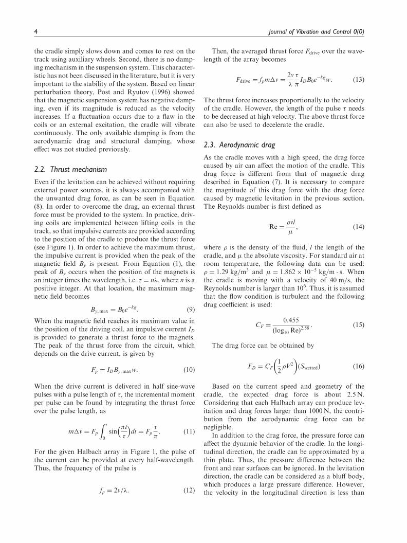
Since the system does not have any damping, it willcontinuously oscillate when the initial condition is notin equilibrium. Figure 4 shows the phase portrait of thesystem (Strogatz, 1994). The amplitude of the velocityis about 0.2m/s, while that of the displacement is0.3 cm. The phase portrait does not show any spiralbehavior, which means that the system does not haveany damping. The center of the ellipse corresponds tothe equilibrium configuration. For a different initialposition, the radius of the ellipse will be changed.This observation is different from that of Post andRyutov (1996), who showed that the system has nega-tive damping-based linear perturbation. However, thenumerical result in Figure 4 shows that the system doesnot have any energy-dissipating mechanism and is neu-trally stable.

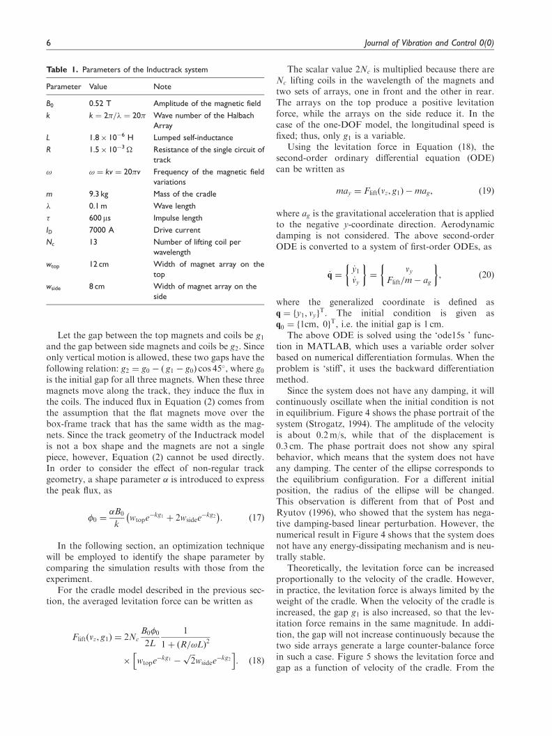
Theoretically, the levitation force can be increasedproportionally to the velocity of the cradle. However,in practice, the levitation force is always limited by theweight of the cradle. When the velocity of the cradle isincreased, the gap g1 is also increased, so that the lev-itation force remains in the same magnitude. In addi-tion, the gap will not increase continuously because thetwo side arrays generate a large counter-balance forcein such a case. Figure 5 shows the levitation force andgap as a function of velocity of the cradle. From the

Table 1. Parameters of the Inductrack system

Parameter Value Note

B0 0.52 T Amplitude of the magnetic field

k k ¼ 2�=� ¼ 20� Wave number of the Halbach

Array

L 1.8� 10�6 H Lumped self-inductance

R 1.5� 10�3 � Resistance of the single circuit of

track

! ! ¼ kv ¼ 20�v Frequency of the magnetic field

variations

m 9.3 kg Mass of the cradle

� 0.1 m Wave length

� 600ms Impulse length

ID 7000 A Drive current

Nc 13 Number of lifting coil per

wavelength

wtop 12 cm Width of magnet array on the

top

wside 8 cm Width of magnet array on the

side





figure, it can be concluded that the cradle shows astable behavior in high velocity.

3.3. 2-DOF model

A 2-DOF model consists of the vertical and the longi-tudinal motions of the cradle. The cradle is consideredas a lumped mass. The main purposes of this model are(1) to identify the unknown parameters, (2) to study theeffect of magnetic drag force and the behavior ofthe cradle under variable velocities, and (3) to modelthe contact conditions between the track and the cradleusing the compliant contact model with inelastic resti-tution as damping.

The configuration of the cradle is the same as withthe 1-DOF model. Accordingly, the levitation force inEquation (18) can be used. In addition to Fy, there

exists a drag force due to the motion of the cradle,which can be obtained from Equation (7) and the con-figuration of the cradle in Figure 3, as

Fdrag ¼ 2NcB0�02L

R=!L

1þ ðR=!LÞ2

� wtope�kg1 þ 2wsidee

�kg2� �

: ð21Þ

By comparing Equation (21) with Equation (18), itcan be easily found that the two side magnets compen-sate the levitation force, while they are accumulateddirectly to the drag force. Thus, the system has moredrag and less levitation than that designed based on theflat magnets on the box-frame track, which is consistentwith the experimental observation (Tung et al., 2001).

In order to overcome the drag force, a thrust force isapplied to the cradle by providing the drive coils withimpulsive current that is synchronized with the positionof the cradle. In practice, three adjacent coils are simul-taneously excited per magnet array in order to increasethe thrust force. The thrust force in Equation (13) isobtained assuming that a single coil is excited when themagnetic field reaches its maximum value. A scalar var-iable is included in order to consider the effect ofthree coils. Accordingly, the thrust force of the cradlein Figure 3 is given as

Fdrive ¼ 2 wtope�kg1 þ 2wsidee

�kg2� � 2vz

�

�

�IDB0: ð22Þ

The thrust force is linearly proportional to the lon-gitudinal velocity, whereas the drag force in Equation(21) is decreased once it reaches the maximum value atthe transient velocity ! ¼ R=L. Thus, it is possible tofind the velocity that makes the drag and thrust be inequilibrium. At that speed, the cradle will move withthe constant speed.

Before presenting the differential equation for the2-DOF model, the method of imposing the contact con-straint is first discussed. The magnetic arrays are notallowed to penetrate the track, which can be imposedusing the following contact constraints:

g1ðtÞ � 0

g2ðtÞ � 0:ð23Þ

A Lagrange multiplier or a penalty method can beused to impose the unilateral boundary condition in thedifferential equation (Haug, 1989). When the Lagrangemultiplier method is applied to the variational princi-ple, the governing equation becomes a differential-algebraic equation, and an additional variable isadded to the system. The advantage of this method isthat it can impose the contact constraint exactly, and

6 7 8 9 10 11

x 10−3

−0.1

−0.05

0

0.05

0.1

0.15

y

Vy

Figure 4. Phase portrait of the 1-DOF model between g1

and vy. The system is neutrally stable.

0 10 20 30 40 500

20

40

60

80

100

120

Vz (m/sec)

2.4

2.0

1.6

1.2

0.8

0.4

0.0

gap (cm)Flift (N)

Flift

gap

Figure 5. Change of levitation force and gap with respect to

longitudinal velocity. Owing to the counter-balance force from

the side arrays, both show a stable behavior.

Kim and Ge 7




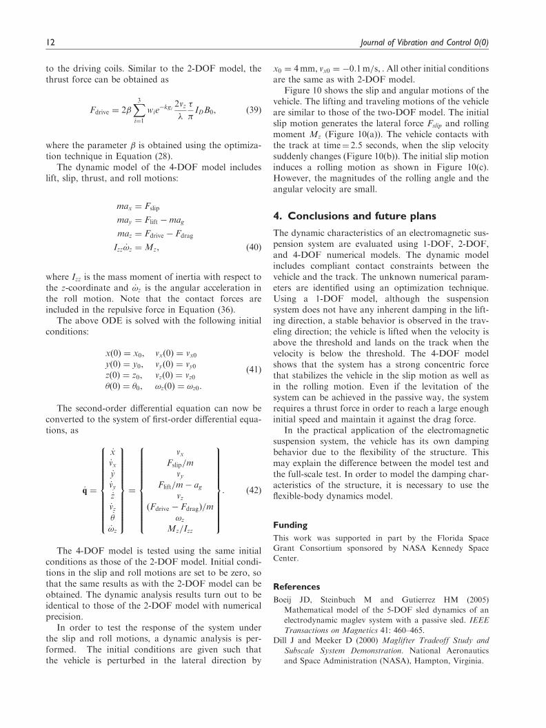
the Lagrange multiplier corresponds to the contactforce. When the penalty method is used, however, noadditional variable is added to the original differentialequation. If the contact condition is violated, then it ispenalized using a large penalty parameter.

In practice, the contact interface between two flexi-ble bodies shows compliant behavior due to thelocal deformation (Hunt and Crossley, 1975). In addi-tion, the restitution is not fully elastic. In thispaper, the compliant contact model with inelasticrestitution as damping is used to impose thecontact condition. The differential equation of thedynamic problem with the penalized contact constraintbecomes

may ¼ Fliftðvz,g1Þ �Fcontðg1, _g1Þ �ffiffiffi2p

Fcontðg2, _g2Þ �mag

maz ¼ Fdriveðvz,g1Þ �Fdragðvz,g1Þ,

ð24Þ

where Fcontð g, _gÞ is defined as

Fcontð g, _gÞ ¼kgþ b _g if g5 0

0 otherwise

, ð25Þ

where k and b are, respectively, the stiffness and damp-ing coefficients of the contact interface. The contactforce for the two side arrays is applied in the directionnormal to the 45� inclined surface, and only the verticalcomponent is considered. The above ordinary differen-tial equation is solved with the following initialconditions:

yð0Þ ¼ y0, vyð0Þ ¼ vy0

zð0Þ ¼ z0, vzð0Þ ¼ vz0 :ð26Þ

The second-order differential equations can now beconverted to the system of first-order differential equa-tions, as

_q ¼

_y

_vy

_z

_vz

8>>><>>>:

9>>>=>>>;¼

vy

½Flift � Fcontð g1, _g1Þ

�ffiffiffi2p

Fcontð g2, _g2Þ�=m� ag

vz

Fdrive � Fdrag

�=m

8>>>>>><>>>>>>:

9>>>>>>=>>>>>>;: ð27Þ

Before the numerical simulation of the 2-DOFmodel, the unknown parameters, � and , need to beidentified. For that purpose, the test results performedby Tung et al. (2001) are utilized. The maximum trav-eling distances for different initial velocities are firstmeasured. The difference between these distances andthose from the dynamic analysis is minimized by

changing the two parameters. The design identificationproblem can then be written as

Minimize f ð�,Þ ¼

ffiffiffiffiffiffiffiffiffiffiffiffiffiffiffiffiffiffiffiffiffiffiffiffiffiffiffiffiffiffiffiffiffiffiffiffiffiffiffiffiffiffiffiffiffiffiX4i¼1

dtesti � d simulationi

�2vuut : ð28Þ

The above minimization problem is solved usingMATLAB ‘fminsearch’ function. The initial valuesare chosen from their ideal cases. Table 2 shows theinitial and optimum values of the parameters. Asexpected, the shape parameter � is reduced from itsideal values, while is increased. At the optimizedvalues of the parameters, the error function f ð�,Þ isreduced significantly.

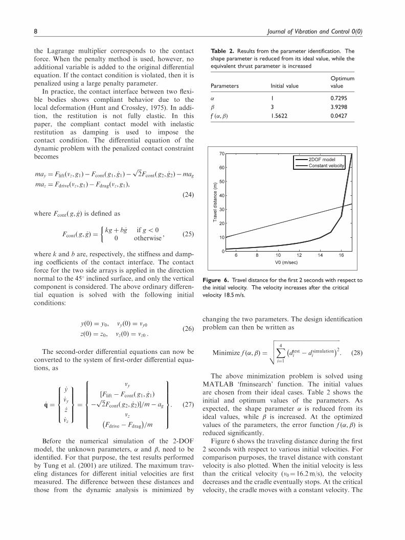
Figure 6 shows the traveling distance during the first2 seconds with respect to various initial velocities. Forcomparison purposes, the travel distance with constantvelocity is also plotted. When the initial velocity is lessthan the critical velocity (v0¼ 16.2m/s), the velocitydecreases and the cradle eventually stops. At the criticalvelocity, the cradle moves with a constant velocity. The

Table 2. Results from the parameter identification. The

shape parameter is reduced from its ideal value, while the

equivalent thrust parameter is increased

Parameters Initial value

Optimum

value

� 1 0.7295

3 3.9298

f ð�,Þ 1.5622 0.0427

Figure 6. Travel distance for the first 2 seconds with respect to

the initial velocity. The velocity increases after the critical

velocity 18.5 m/s.





velocity increases exponentially when the initial velocityis above the critical value.

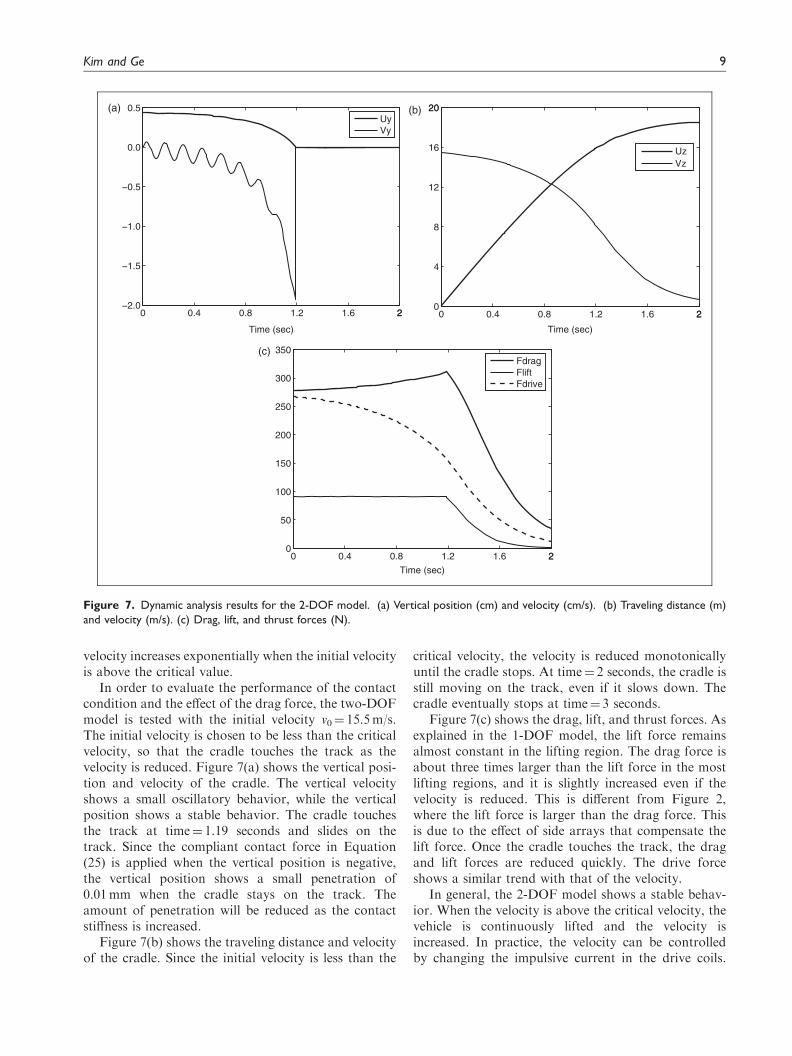
In order to evaluate the performance of the contactcondition and the effect of the drag force, the two-DOFmodel is tested with the initial velocity v0¼ 15.5m/s.The initial velocity is chosen to be less than the criticalvelocity, so that the cradle touches the track as thevelocity is reduced. Figure 7(a) shows the vertical posi-tion and velocity of the cradle. The vertical velocityshows a small oscillatory behavior, while the verticalposition shows a stable behavior. The cradle touchesthe track at time¼ 1.19 seconds and slides on thetrack. Since the compliant contact force in Equation(25) is applied when the vertical position is negative,the vertical position shows a small penetration of0.01mm when the cradle stays on the track. Theamount of penetration will be reduced as the contactstiffness is increased.

Figure 7(b) shows the traveling distance and velocityof the cradle. Since the initial velocity is less than the

critical velocity, the velocity is reduced monotonicallyuntil the cradle stops. At time¼ 2 seconds, the cradle isstill moving on the track, even if it slows down. Thecradle eventually stops at time¼ 3 seconds.

Figure 7(c) shows the drag, lift, and thrust forces. Asexplained in the 1-DOF model, the lift force remainsalmost constant in the lifting region. The drag force isabout three times larger than the lift force in the mostlifting regions, and it is slightly increased even if thevelocity is reduced. This is different from Figure 2,where the lift force is larger than the drag force. Thisis due to the effect of side arrays that compensate thelift force. Once the cradle touches the track, the dragand lift forces are reduced quickly. The drive forceshows a similar trend with that of the velocity.

In general, the 2-DOF model shows a stable behav-ior. When the velocity is above the critical velocity, thevehicle is continuously lifted and the velocity isincreased. In practice, the velocity can be controlledby changing the impulsive current in the drive coils.

(a) (b)

(c)

0 0.4 0.8 1.2 1.6 22−2.0

−1.5

−1.0

−0.5

0.0

0.5

Time (sec)

UyVy

0 0.4 0.8 1.2 1.6 220

4

8

12

16

2020

Time (sec)

UzVz

0 0.4 0.8 1.2 1.6 220

50

100

150

200

250

300

350

Time (sec)

FdragFliftFdrive

Figure 7. Dynamic analysis results for the 2-DOF model. (a) Vertical position (cm) and velocity (cm/s). (b) Traveling distance (m)

and velocity (m/s). (c) Drag, lift, and thrust forces (N).

Kim and Ge 9




When the velocity is reduced, the vehicle lands on thetrack and eventually stops.

3.4. 4-DOF model

In 1- and 2-DOF models, the cradle is assumed to bea lumped mass structure. The purpose of the 4-DOFmodel is to evaluate the rigid body behavior of thesystem. The cradle can move in the z-direction(thrust), y-direction (lift), x-direction (slip), androtate in the z-direction (roll). Figure 8 shows thecomputational model with coordinate systems. Theglobal coordinate X–Y is fixed on the track, whilethe local coordinate X’–Y’ is fixed on the cradle.Both local and global coordinates have the sameorigin when the three magnets have the same gap(1.0 cm) with respect to the track. In order to simplifythe contact calculation, the geometry of the magnets isrepresented by a point. In addition, it is assumed thatthe direction of the lift force is always normal to thetrack, not to the magnets. The effect of this assump-tion is not significant because the roll angle is sup-posed to be small.

The magnetic force depends on the gap between themagnets and the induced coils. The location of the mag-nets is calculated based on the local-to-global coordi-nate transformation. When the local coordinate of themagnet array i is given as r0i, the global coordinate canbe obtained from

ri ¼ r0 þ AðÞ � r0i, i ¼ 1, 2, 3, ð29Þ

where r0 ¼ ðx, yÞ is the position of the origin of the localcoordinate, and AðÞ is the rotational transformationmatrix defined as

AðÞ ¼cos � sin sin cos

� �: ð30Þ

First, the locations of three magnets are calculatedfrom the geometry of the cradle in the local coordinate,and then, their global coordinates are calculated fromEquation (29).

After calculating the global coordinate of the mag-nets, the gap between the magnets and the track can becalculated from the geometric relation. In order tomake the procedure general, a concept from solidmechanics is adopted (Kim et al., 2000). Let ri be thelocation of the magnet array i, and a1i and a2i be thecoordinates of two end points of the track (seeFigure 9). The segment of the track below the magnetsis a straight line. The two end points are ordered suchthat the magnets should be on the left side when wego from a1i to a2i . If the magnets are on the right side,it is considered that they penetrate the track and thecontact force is applied to push them out. First, the unittangent and normal vector to the track can be obtainedby

ti ¼a2i � a1i

ka2i � a1i k, ni ¼ e3 � ti, ð31Þ

where e3 is the unit vector in the z-coordinate, i.e.(0, 0, 1). Then, the gap between magnets and trackcan be calculated from

gi ¼ ri � a1i �

� ni � 0: ð32Þ

In addition, the rate of gap distance can becalculated by differentiating the relation inEquation (29) and using the property that the track isfixed, as

_gi ¼ v0 þ _AðÞ � r0i

� �� ni, ð33Þ

where

_AðÞ ¼ !z� sin � cos cos � sin

� �: ð34Þ

X, X'

Y, Y'

θ

Track with Coils

F1

F2 F3

g1

g2 g3

Figure 8. Four-DOF Inductrack dynamic model. The X–Y

coordinate is fixed on the track, while the X’–Y’ coordinate is

fixed on the cradle.

Magnets

Track

ri

1ia 2

ia

ign

tcr

Figure 9. Contact condition between magnets and track.

The magnets are considered as a point. The gap gi must be

non-negative.





When these three magnets move along the track,they induce the flux in the coils. In the 4-DOF model,the peak flux can be obtained by

�0 ¼�B0

k

X3i¼1

wie�kgi : ð35Þ

As with the 2-DOF model, the shape parameter � isincluded. Then, the repulsive force at each magnetarray can be written as

Fi ¼ wie�kgi

B0�02L

2Nc

1þ ðR=!LÞ2� Fcontð gi, _giÞ, i ¼ 1, 2, 3:

ð36Þ

These three repulsive forces, as illustrated inFigure 8, contribute to the lift and slip force of

the cradle. Since it is assumed that these forces areapplied in the direction normal to the track, the liftand slip forces can be obtained as

Flift ¼ F1 � ðF2 þ F3Þ cosð45�Þ

Fslip ¼ ðF3 � F2Þ sinð45�Þ:

ð37Þ

Different from the lift and slip forces inEquation (37), the drag force is obtained by addingthe contribution from the three magnet arrays, as

Fdrag ¼X3i¼1

wie�kgi � 2Nc

B0�02L

R=!L

1þ ðR=!LÞ2: ð38Þ

In order to overcome this drag force, the thrust forceis applied to the cradle by providing impulsive current

(a) (b)

(c)

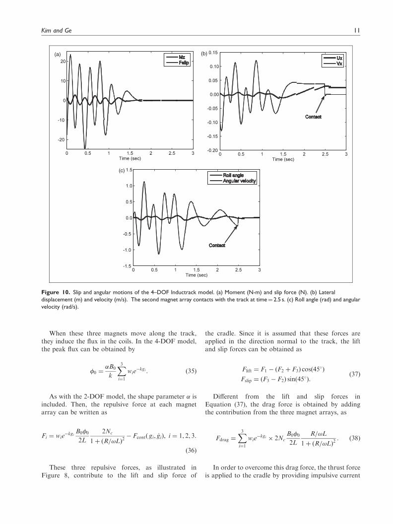
Figure 10. Slip and angular motions of the 4–DOF Inductrack model. (a) Moment (N-m) and slip force (N). (b) Lateral

displacement (m) and velocity (m/s). The second magnet array contacts with the track at time¼ 2.5 s. (c) Roll angle (rad) and angular

velocity (rad/s).

Kim and Ge 11




to the driving coils. Similar to the 2-DOF model, thethrust force can be obtained as

Fdrive ¼ 2X3i¼1

wie�kgi

2vz�

�

�IDB0, ð39Þ

where the parameter is obtained using the optimiza-tion technique in Equation (28).

The dynamic model of the 4-DOF model includeslift, slip, thrust, and roll motions:

max ¼ Fslip

may ¼ Flift �mag

maz ¼ Fdrive � Fdrag

Izz _!z ¼Mz, ð40Þ

where Izz is the mass moment of inertia with respect tothe z-coordinate and _!z is the angular acceleration inthe roll motion. Note that the contact forces areincluded in the repulsive force in Equation (36).

The above ODE is solved with the following initialconditions:

xð0Þ ¼ x0, vxð0Þ ¼ vx0yð0Þ ¼ y0, vyð0Þ ¼ vy0zð0Þ ¼ z0, vzð0Þ ¼ vz0ð0Þ ¼ 0, !zð0Þ ¼ !z0:

ð41Þ

The second-order differential equation can now beconverted to the system of first-order differential equa-tions, as

_q ¼

_x_vx_y_vy_z_vz__!z

8>>>>>>>>>><>>>>>>>>>>:

9>>>>>>>>>>=>>>>>>>>>>;

¼

vxFslip=m

vyFlift=m� ag

vzðFdrive � FdragÞ=m

!z

Mz=Izz

8>>>>>>>>>><>>>>>>>>>>:

9>>>>>>>>>>=>>>>>>>>>>;

: ð42Þ

The 4-DOF model is tested using the same initialconditions as those of the 2-DOF model. Initial condi-tions in the slip and roll motions are set to be zero, sothat the same results as with the 2-DOF model can beobtained. The dynamic analysis results turn out to beidentical to those of the 2-DOF model with numericalprecision.

In order to test the response of the system underthe slip and roll motions, a dynamic analysis is per-formed. The initial conditions are given such thatthe vehicle is perturbed in the lateral direction by

x0 ¼ 4mm, vx0 ¼ �0:1m=s, . All other initial conditionsare the same as with 2-DOF model.

Figure 10 shows the slip and angular motions of thevehicle. The lifting and traveling motions of the vehicleare similar to those of the two-DOF model. The initialslip motion generates the lateral force Fslip and rollingmoment Mz (Figure 10(a)). The vehicle contacts withthe track at time¼ 2.5 seconds, when the slip velocitysuddenly changes (Figure 10(b)). The initial slip motioninduces a rolling motion as shown in Figure 10(c).However, the magnitudes of the rolling angle and theangular velocity are small.

4. Conclusions and future plans

The dynamic characteristics of an electromagnetic sus-pension system are evaluated using 1-DOF, 2-DOF,and 4-DOF numerical models. The dynamic modelincludes compliant contact constraints between thevehicle and the track. The unknown numerical param-eters are identified using an optimization technique.Using a 1-DOF model, although the suspensionsystem does not have any inherent damping in the lift-ing direction, a stable behavior is observed in the trav-eling direction; the vehicle is lifted when the velocity isabove the threshold and lands on the track when thevelocity is below the threshold. The 4-DOF modelshows that the system has a strong concentric forcethat stabilizes the vehicle in the slip motion as well asin the rolling motion. Even if the levitation of thesystem can be achieved in the passive way, the systemrequires a thrust force in order to reach a large enoughinitial speed and maintain it against the drag force.

In the practical application of the electromagneticsuspension system, the vehicle has its own dampingbehavior due to the flexibility of the structure. Thismay explain the difference between the model test andthe full-scale test. In order to model the damping char-acteristics of the structure, it is necessary to use theflexible-body dynamics model.

Funding

This work was supported in part by the Florida SpaceGrant Consortium sponsored by NASA Kennedy Space

Center.

References

Boeij JD, Steinbuch M and Gutierrez HM (2005)

Mathematical model of the 5-DOF sled dynamics of an

electrodynamic maglev system with a passive sled. IEEE

Transactions on Magnetics 41: 460–465.Dill J and Meeker D (2000) Maglifter Tradeoff Study and

Subscale System Demonstration. National Aeronautics

and Space Administration (NASA), Hampton, Virginia.





Halbach K (1985) Application of permanent magnets inaccelerators and electron storage rings. Journal ofApplied Physics 57: 3605–3608.

Haug EJ (1989) Computer-Aided Kinematics and Dynamics ofMechanical Systems. Volume 1: Basic Methods. Boston,MA: Allyn and Bacon.

Hunt KH and Crossley FRE (1975) Coefficient of restitution

interpreted as damping in vibroimpact. Applied Mechanics42: 440–445.

Kalsi SS (1994) Superconductive electromagnetic suspension

for Grumman maglev concept. In: Groom NJ (ed.) SecondInternational Symposium on Magnetic SuspensionTechnology Part 1. Hapton: NASA, pp.197–211.

Kim NH, Choi KK, Chen JS and Park YH (2000) Meshlessshape design sensitivity analysis and optimization for con-tact problems with friction. Computational Mechanics 25:

157–168.Luerkin RF (1994) Transrapid (the first high-speed maglev

train system certified and ready for application):Development status and prospect for development.

In: Groom NJ (ed.) Second International Symposium onMagnetic Suspension Technology Part 1. Hapton: NASA,pp.77–91.

Matsue H, Demachi K and Miya K (2001) Numerical analy-

sis of the superconducting magnet outer vessel of a maglev

train by a structural and electromagnetic coupling method.

Physica C Superconductivity 357–360: 874–877.Post RF and Ryutov DD (1996) Inductrack Concept: A New

Approach to Magnetic Levitation. Lawrence Livermore

National Laboratory, Livermore.

Post RF and Ryutov DD (2000) The Inductrack: a simpler

approach to magnetic levitation. IEEE Transactions on

Applied Superconductivity 10: 901–904.Powell JR and Danby GR (1971) Magnetic suspension for

levitated tracked vehicle. Cryogenics 11: 192–204.Rote DM and Cai Y (2002) Review of dynamic stability of

repulsive-force maglev suspension systems. IEEE

Transactions on Magnetics 38: 1383–1390.Strogatz SH (1994) Nonlinear Dynamics and Chaos: With

Applications to Physics, Biology, Chemistry, and

Engineering. New York: Addison-Wesley.Tung LS, Post RF and Martinez-Frias J (2001) Final Progress

Report for the NASA Inductrack Model Rocket launcher at

the Lawrence Livermore National Laboratory. Lawrence

Livermore National Laboratory, Livermore.

Kim and Ge 13



Documents

Dynamic modeling of electromagnetic suspension system