Dynamic Modeling and Control of Binary Distillation … Modeling and Control of Binary Distillation Column ) )

IJSRD - International Journal for Scientific Research & Development| Vol. 4, Issue 02, 2016 | ISSN (online): 2321-0613

All rights reserved by www.ijsrd.com 1779

Dynamic Modeling and Control of Binary Distillation Column Mehul Pragjibhai Girnari1 Prof. Vinod P. Patel2

1,2Department of Instrumentation and Control Engineering 1,2L.D. College of Engineering, Ahmedabad, 380015

Abstract— Distillation column has always been and will

continue to be one of the most important thermal separation

equipment used in various types of industries for various

applications, like in oil refineries, in water purification/

desalinization plants, in pharmaceutical industries etc.

Modelling and simulation of distillation column are not new

to the process and control engineer. The model used for

distillation column varies from the simple to quite complex,

depending on the assumption made in the material balance

and energy balance equations to describe the distillation

column behavior. This paper discuss about the dynamic

modelling of continuous binary distillation column in

Matlab tool and the response analysis while varying the

assumptions made while developing the dynamic model.

This paper also discuss about the tuning of PID controller

using different tuning methods which is job of control

engineer.

Key words: Binary, Distillation, Dynamic model, S-function

I. INTRODUCTION

Distillation is a thermal separation method for separating

mixtures of two or more substances into its component

fractions of desired concentration, based on differences in

volatilities or the boiling point difference of these

components by the application and removal of heat.

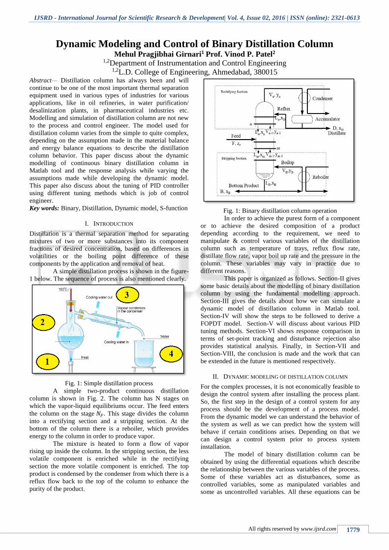
A simple distillation process is shown in the figure-

1 below. The sequence of process is also mentioned clearly.

Fig. 1: Simple distillation process

A simple two-product continuous distillation

column is shown in Fig. 2. The column has N stages on

which the vapor-liquid equilibriums occur. The feed enters

the column on the stage 𝑁𝐹. This stage divides the column

into a rectifying section and a stripping section. At the

bottom of the column there is a reboiler, which provides

energy to the column in order to produce vapor.

The mixture is heated to form a flow of vapor

rising up inside the column. In the stripping section, the less

volatile component is enriched while in the rectifying

section the more volatile component is enriched. The top

product is condensed by the condenser from which there is a

reflux flow back to the top of the column to enhance the

purity of the product.

Fig. 1: Binary distillation column operation

In order to achieve the purest form of a component

or to achieve the desired composition of a product

depending according to the requirement, we need to

manipulate & control various variables of the distillation

column such as temperature of trays, reflux flow rate,

distillate flow rate, vapor boil up rate and the pressure in the

column. These variables may vary in practice due to

different reasons.

This paper is organized as follows. Section-II gives

some basic details about the modelling of binary distillation

column by using the fundamental modelling approach.

Section-III gives the details about how we can simulate a

dynamic model of distillation column in Matlab tool.

Section-IV will show the steps to be followed to derive a

FOPDT model. Section-V will discuss about various PID

tuning methods. Section-VI shows response comparison in

terms of set-point tracking and disturbance rejection also

provides statistical analysis. Finally, in Section-VII and

Section-VIII, the conclusion is made and the work that can

be extended in the future is mentioned respectively.

II. DYNAMIC MODELING OF DISTILLATION COLUMN

For the complex processes, it is not economically feasible to

design the control system after installing the process plant.

So, the first step in the design of a control system for any

process should be the development of a process model.

From the dynamic model we can understand the behavior of

the system as well as we can predict how the system will

behave if certain conditions arises. Depending on that we

can design a control system prior to process system

installation.

The model of binary distillation column can be

obtained by using the differential equations which describe

the relationship between the various variables of the process.

Some of these variables act as disturbances, some as

controlled variables, some as manipulated variables and

some as uncontrolled variables. All these equations can be

Dynamic Modeling and Control of Binary Distillation Column

(IJSRD/Vol. 4/Issue 02/2016/499)


derived with the help of the laws of thermodynamics

(energy balance equations) and mass-balance equations.

Modeling of the distillation column is often

classified into three types as describe below:

A. Fundamental modeling method

In fundamental modelling method, the model is developed

based on the physical properties of the system, such as the

preservation of energy, mass and momentum. This method

of modeling has an advantage of global validity, accuracy

and it gives more detailed process understanding. However,

this modeling method is quite complex for the controller

design, because it requires a huge amount of computation

and simplifications.

B. Empirical modeling method

The empirical modeling utilizes the input and output data

from the operation of the column to build the relationship

between the input and the output. This method is also known

as “Black box modeling” because inner dynamics are not

considered. With this type of modelling, the understanding

of the inner dynamics of the column does not required. So,

the computation can be reduced.

But by using this technique, we must carry out

experiments on the real distillation column, and the results

may not be applied for another distillation column, even the

results from one distillation column can be different if the

distillation column’s conditions are different between the

experiment and the real operation of the distillation column.

C. Hybrid modeling method

The hybrid modeling (or the ‘grey-box’ modeling) combines

the fundamental modeling and the empirical modeling. This

method utilizes the advantages of both methods

(fundamental modeling and empirical modeling), but the

critical thing is that we must to decide for which part of the

model do we need to use fundamental modelling and for

which part to use empirical modelling.

Here, for this work I used fundamental modeling

method for the development of dynamic model for the

continuous binary distillation column. In order to develop

this model we need to make some assumptions. So, next

section will describe the assumption need to be made.

In the model of the distillation column the

following assumptions are made:

1) The feed contains only two components (Binary

mixture).

2) The column is perfectly insulated.

3) Constant relative volatility.

4) Constant molar flows.

5) No vapor holds up.

6) All the trays are ideal (100% efficient)

7) Linear liquid dynamics.

8) Equilibrium on all stages.

9) Pressure inside the column is fixed.

10) Total condenser and reboiler.

Here, for fundamental modeling, we will divide the

distillation model in four envelopes, which are:

1) Condenser

2) Reboiler

3) Feed tray

4) All other trays (except feed tray)

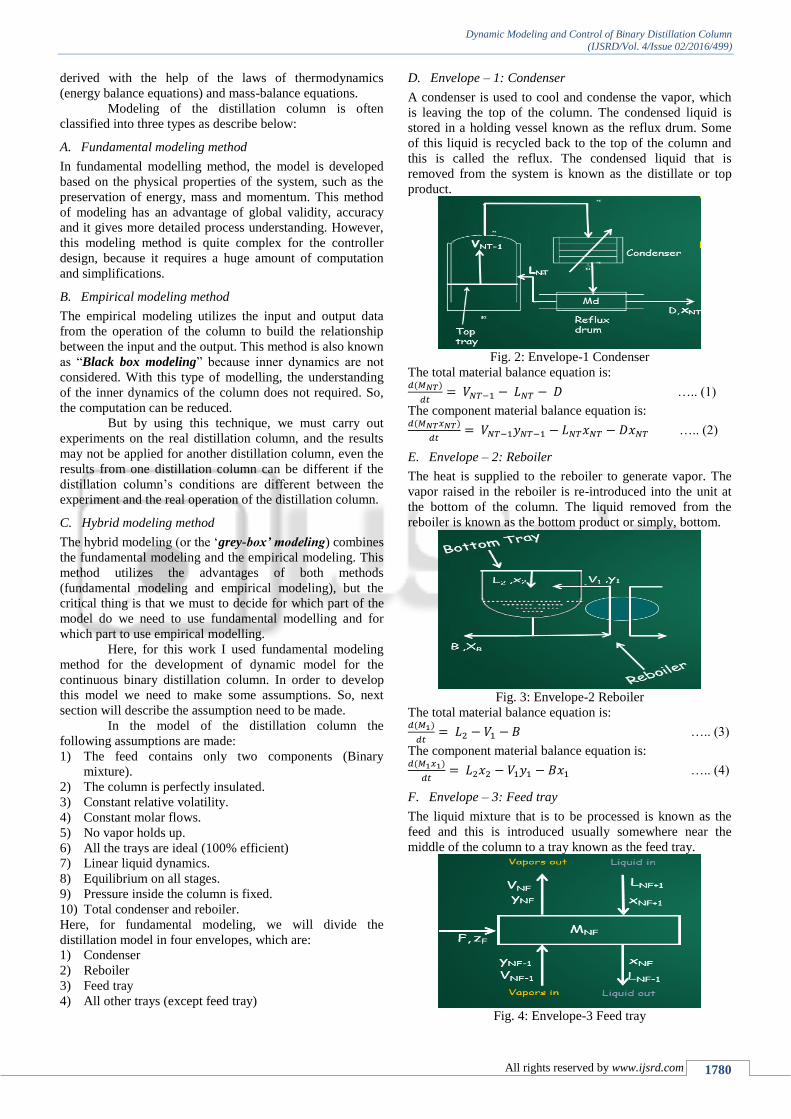
D. Envelope – 1: Condenser

A condenser is used to cool and condense the vapor, which

is leaving the top of the column. The condensed liquid is

stored in a holding vessel known as the reflux drum. Some

of this liquid is recycled back to the top of the column and

this is called the reflux. The condensed liquid that is

removed from the system is known as the distillate or top

product.

Fig. 2: Envelope-1 Condenser

The total material balance equation is: 𝑑(𝑀𝑁𝑇)

𝑑𝑡= 𝑉𝑁𝑇−1 − 𝐿𝑁𝑇 − 𝐷 ….. (1)

The component material balance equation is: 𝑑(𝑀𝑁𝑇𝑥𝑁𝑇)

𝑑𝑡= 𝑉𝑁𝑇−1𝑦𝑁𝑇−1 − 𝐿𝑁𝑇𝑥𝑁𝑇 − 𝐷𝑥𝑁𝑇 ….. (2)

E. Envelope – 2: Reboiler

The heat is supplied to the reboiler to generate vapor. The

vapor raised in the reboiler is re-introduced into the unit at

the bottom of the column. The liquid removed from the

reboiler is known as the bottom product or simply, bottom.

Fig. 3: Envelope-2 Reboiler

The total material balance equation is: 𝑑(𝑀1)

𝑑𝑡= 𝐿2 − 𝑉1 − 𝐵 ….. (3)

The component material balance equation is: 𝑑(𝑀1𝑥1)

𝑑𝑡= 𝐿2𝑥2 − 𝑉1𝑦1 − 𝐵𝑥1 ….. (4)

F. Envelope – 3: Feed tray

The liquid mixture that is to be processed is known as the

feed and this is introduced usually somewhere near the

middle of the column to a tray known as the feed tray.

Fig. 4: Envelope-3 Feed tray




The total material balance equation at the feed stage (NF), 𝑑(𝑀𝑁𝐹)

𝑑𝑡= 𝐿𝑁𝐹+1− 𝐿𝑁𝐹 + 𝑉𝑁𝐹−1 − 𝑉𝑁𝐹 + 𝐹 ….. (5)

The total material balance equation at the feed stage (NF), 𝑑(𝑀𝑁𝐹𝑥𝑁𝐹)

𝑑𝑡= 𝐿𝑁𝐹+1𝑥𝑁𝐹+1 − 𝐿𝑁𝐹𝑥𝑁𝐹 + 𝑉𝑁𝐹−1𝑦𝑁𝐹−1 −

𝑉𝑁𝐹𝑦𝑁𝐹−1 + 𝐹𝑧𝐹 ….. (6)

Where,

F is the feed flow rate,

𝑧𝐹 is the concentration of the light component in

feed

G. Envelope – 4: Other trays (except feed tray)

Fig. 5. Envelope-4 all other general trays (except feed tray)

The total material balance equations on stage i is given by, 𝑑𝑀𝑖

𝑑𝑡= 𝐿𝑖+1 − 𝐿𝑖 + 𝑉𝑖−1 − 𝑉𝑖 ….. (7)

Where,

𝑀𝑖 is liquid hold up on tray 𝑖 , 𝐿𝑖 is liquid flow rate,

𝑉𝑖 is vapor flow rate that comes toward tray i.

The material balance for the light component on tray (i) is

given by, 𝑑(𝑀𝑖 𝑥𝑖)

𝑑𝑡= 𝐿𝑖+1𝑥𝑖+1 − 𝐿𝑖𝑥𝑖 + 𝑉𝑖−1𝑦𝑖−1 − 𝑉𝑖𝑦𝑖 ….. (8)

Where,

𝑥𝑖 & 𝑦𝑖 is the composition of the light and heavy

component on a tray (i) respectively.

The composition of the heavy component is related

to the composition of the light component via the relative

volatility, which is given by the equation,

𝑦𝑖 = 𝛼𝑥1

1+(𝛼−1)𝑥1 ….. (9)

The liquid flow dynamics is considered due to its important

effect on the initial response of the distillation column. The

liquid holdup given by the following equations,

𝐿𝑖 = 𝐿0𝑏 +𝑀𝑖−𝑀0𝑖

𝜏+ (𝑉𝑖+1 − 𝑉0)𝜆 ….. (10)

For I from 2 to 𝑁𝐹 and

𝐿𝑖 = 𝐿0 +𝑀𝑖−𝑀0𝑖

𝜏+ (𝑉𝑖+1 − 𝑉0𝑡)𝜆 ….. (11)

For I from 𝑁𝐹 + 1 to 𝑁𝑇 − 1.

Where,

𝐿0 is the nominal reflux flow,

𝑀0𝑖 is the nominal re boiler hold up (kmol) on stage

i.

𝜏 is the time constant for liquid dynamics

=0.063(min)

𝜆 represents the effect of vapor flow on liquid flow.

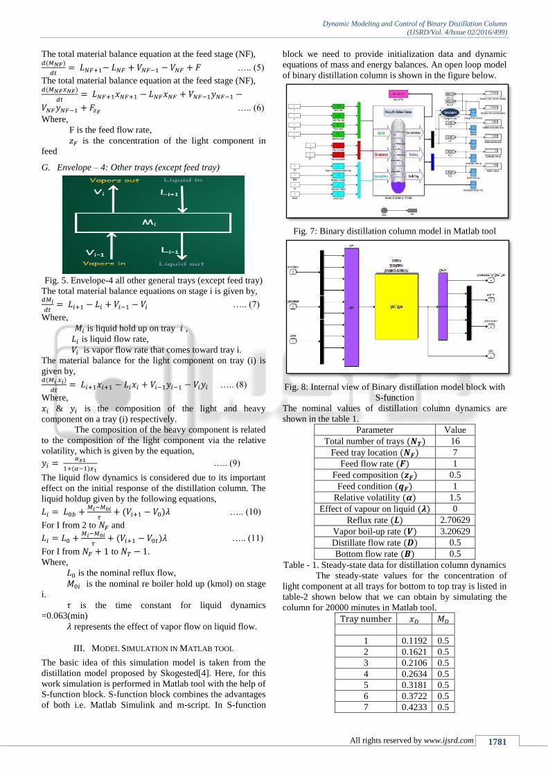
III. MODEL SIMULATION IN MATLAB TOOL

The basic idea of this simulation model is taken from the

distillation model proposed by Skogested[4]. Here, for this

work simulation is performed in Matlab tool with the help of

S-function block. S-function block combines the advantages

of both i.e. Matlab Simulink and m-script. In S-function

block we need to provide initialization data and dynamic

equations of mass and energy balances. An open loop model

of binary distillation column is shown in the figure below.

Fig. 7: Binary distillation column model in Matlab tool

Fig. 8: Internal view of Binary distillation model block with

S-function

The nominal values of distillation column dynamics are

shown in the table 1.

Parameter Value

Total number of trays (𝑵𝑻) 16

Feed tray location (𝑵𝑭) 7

Feed flow rate (𝑭) 1

Feed composition (𝒛𝑭) 0.5

Feed condition (𝒒𝑭) 1

Relative volatility (𝜶) 1.5

Effect of vapour on liquid (𝝀) 0

Reflux rate (𝑳) 2.70629

Vapor boil-up rate (𝑽) 3.20629

Distillate flow rate (𝑫) 0.5

Bottom flow rate (𝑩) 0.5

Table - 1. Steady-state data for distillation column dynamics

The steady-state values for the concentration of

light component at all trays for bottom to top tray is listed in

table-2 shown below that we can obtain by simulating the

column for 20000 minutes in Matlab tool.

Tray number 𝑥𝐷 𝑀𝐷

1 0.1192 0.5

2 0.1621 0.5

3 0.2106 0.5

4 0.2634 0.5

5 0.3181 0.5

6 0.3722 0.5

7 0.4233 0.5




8 0.4581 0.5

9 0.4997 0.5

10 0.5478 0.5

11 0.6015 0.5

12 0.6590 0.5

13 0.7182 0.5

14 0.7764 0.5

15 0.8312 0.5

16 0.8807 0.5

Table - 2. Light component concentration values and hold-

up on each tray at steady-state

The relative volatility is ultimately the difference of

boiling points of MVC (More Volatile Component) and

LVC (Less Volatile Component).

The table-3. Shows values of an optimal relative

volatility (𝛼) for different binary mixtures as listed. You

need to specify that particular value of relative volatility for

particular binary mixture in the simulation model.

MVC

(boiling point

in ℃)

LVC

(boiling point in

℃)

Optimal relative

volatility (𝛼)

Benzene

(80.1) Toluene (110.6) 2.34

Toluene

(110.6) p-Xylene (138.3) 2.31

Benzene

(80.6) p-Xylene (138.3) 4.82

m-Xylene

(139.1 p-Xylene (138.3) 1.02

Pentane

(36.0) Hexane (68.7) 2.59

Hexane

(68.7) Heptane (98.5) 2.45

Hexane

(68.7) p-Xylene (138.3) 7.0

Ethanol

(78.4)

iso-Propanol

(82.3) 1.17

iso-Propanol

(82.3) n-Propanol (97.3) 1.78

Ethanol

(78.4) n-Propanol (97.3) 2.10

Methanol

(64.6) Ethanol (78.4) 1.56

Methanol

(64.6)

iso-Propanol

(82.3) 2.26

Chloroform

(61.2) Acetic acid (118.1) 6.15

Table - 3. Some optimal relative volatilities that are used

for distillation process design

The upcoming figures will show how the

concentration of light component at condenser and reboiler

varies when we vary variation in the different variables.

Fig. 9: Change in concentration due to 1% increase in reflux

flow rate (L)

Figure. 10: Change in concentration due to 1% increase in

vapor flow rate (V)

Fig. 11: Change in concentration due to 1% increase in feed

flow rate (F)

Fig. 12: Change in concentration due to 1% increase in feed

composition (𝑧𝐹)




From the above responses, it is clear that the change in the

concentration of light component at condenser as well as at

reboiler is significant due to the 1% variation in the feed

composition (𝑧𝐹) as compared to the same amount of

variation in the feed flow rate (𝐹).

Fig. 13: Change in concentration due to 1% increase in

relative volatility (alpha)

Fig. 14: Change in concentration due to feed tray location

(𝑁𝐹)is changed to 4 from 7

If the condition of feed gets changed then how the

concentration of light component gets affected that is shown

in the figure below.

Fig. 15: Change in concentration due to 1% increase in

𝑞𝐹 (𝑞𝐹 = 1.01)

Here, the value of 𝑞𝐹 indicates whether the feed liquid is

completely saturated or not. i.e. 𝑞𝐹 = 1 for saturated feed.

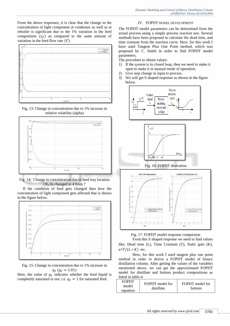
IV. FOPDT MODEL DEVELOPMENT

The FOPDT model parameters can be determined from the

actual process using a simple process reaction test. Several

methods have been proposed to calculate the dead time, and

time constant from the reaction curve. Here, for this work I

have used Tangent Plus One Point method, which was

proposed by C. Smith in order to find FOPDT model

parameters.

The procedure to obtain values:

1) If the system is in closed loop, then we need to make it

open to make it in manual mode of operation.

2) Give step change in input to process.

3) We will get S shaped response as shown in the figure

below.

Fig. 16: FOPDT derivation

Fig. 17: FOPDT model response comparison

From this S shaped response we need to find values

like, Dead time (L), Time Constant (T), Static gain (K),

a=𝑇/(𝐿 ∗ 𝐾) etc.

Here, for this work I used tangent plus one point

method in order to derive a FOPDT model of binary

distillation column. After getting the values of the variables

mentioned above, we can get the approximated FOPDT

model for distillate and bottom product compositions as

listed in table-4.

FOPDT

model

equation

FOPDT model for

distillate

FOPDT model for

bottom




𝐺(𝑠)

=𝑘𝑒−𝐿𝑠

𝑇𝑠 + 1

𝐺(𝑠)

=0.0427𝑒−(2.4115)𝑠

(11.3423)𝑠 + 1

𝐺(𝑠)

=0.0573𝑒−(1.9776)𝑠

([11.7761)𝑠 + 1

Table. 4: FOPDT model equations

V. PID TUNING METHODS

The tuning of PID controller refers to the process of finding

the value of the PID parameter (𝑛𝑎𝑚𝑒𝑙𝑦 𝐾𝑝, 𝐾𝑖 , 𝐾𝑑), which

can provide optimum performances.

The oldest method is trial and error method, which

is simplest and easiest method but the problem is that it is

very time consuming and not reliable. Instead of that, there

are various methods available for PID tuning some of them

are listed below [11].

1) Ziegler-Nichols open loop test tuning method

2) Cohen-Coon tuning method

3) Internal Model Control tuning method

4) ITAE tuning method

5) Lambda tuning method

Controller

type

𝑇𝑢𝑛𝑖𝑛𝑔 𝑝𝑎𝑟𝑎𝑚𝑒𝑡𝑒𝑟𝑠

𝐾𝑝 𝜏𝑖 𝜏𝑑

P 1

a Very large 0

PI 0.9

a 3L 0

PID 1.2

a 2L

L

2

Table. 5: Ziegler-Nichols open loop test tuning method

Controller

type


𝐾𝑝 𝜏𝑖 𝜏𝑑

P (

1

𝑎) (1

+0.35𝜏

1 − 𝜏)

Very large 0

PI (

0.9

𝑎) (1

+0.92𝜏

1 − 𝜏)

3.3 − 3𝜏

1 + 1.2𝜏𝐿 0

PD (

1.24

𝑎) (1

+0.13𝜏

1 − 𝜏)

Very large 0.27 − 0.36𝜏

1 − 0.87𝜏𝐿

PID (

1.35

𝑎) (1

+0.18𝜏

1 − 𝜏)

2.5 − 2𝜏

1 − 0.39𝜏𝐿

0.37 − 0.37𝜏

1 − 0.81𝜏𝐿

Table 6. Cohen-Coon tuning method

Controller

type


𝑘𝑘𝑐 𝜏𝑖 𝜏𝑑

PI 2𝜏 + 𝜃

2𝜆 𝜏 +

𝜃

2 0

PID 2𝜏 + 𝜃

2(𝜆 + 𝜃) 𝜏 +

𝜃

2

𝜏𝜃

2𝜏 + 𝜃

Table 7. Internal Model Control (IMC) tuning method

Controller

type


𝑘𝑘𝑐 𝜏

𝜏𝑖

𝜏𝑑

𝜏

PI

setpoint 0.586 (𝜃

𝜏)

−0.916

1.030

− 0.165 (𝜃

𝜏)

−

PID

setpoint 0.965 (𝜃

𝜏)

−0.850

0.796

− 0.1465 (𝜃

𝜏)

0.308 (𝜃

𝜏)

−0.929

PIdisturban

ce 0.859 (𝜃

𝜏)

−0.977

0.674 (𝜃

𝜏)

−0.680

−

PID-

disturbance 1.357 (𝜃

𝜏)

−0.947

0.842 (𝜃

𝜏)

−0.738

0.381 (𝜃

𝜏)

−0.995

Table 8. ITAE tuning method

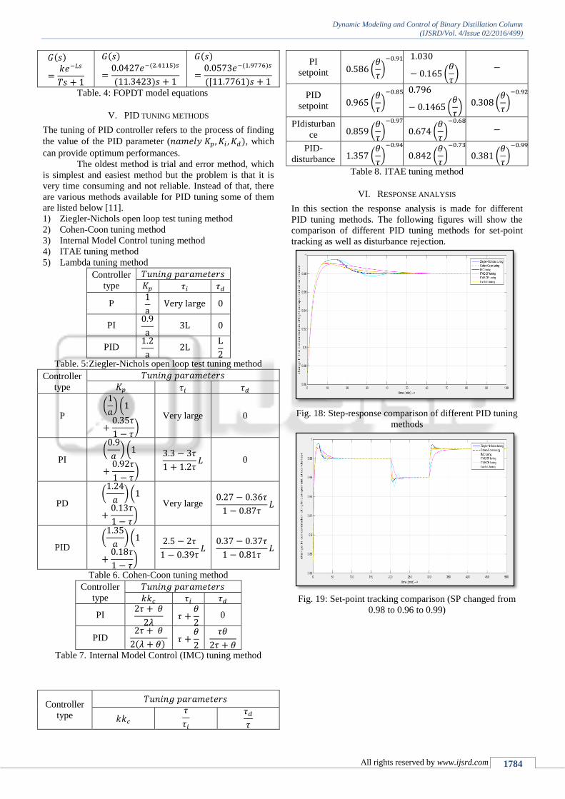
VI. RESPONSE ANALYSIS

In this section the response analysis is made for different

PID tuning methods. The following figures will show the

comparison of different PID tuning methods for set-point

tracking as well as disturbance rejection.

Fig. 18: Step-response comparison of different PID tuning

methods

Fig. 19: Set-point tracking comparison (SP changed from

0.98 to 0.96 to 0.99)




Fig. 20: Disturbance rejection comparison (first 10%

decrease & then 10% increase in Feed flow rate)


decrease & then 10% increase in Feed composition)


decrease & then 10% increase in Feed condition)


decrease & then 10% increase in reflux rate)

Figure 24. Disturbance rejection comparison (first 10%

decrease & then 10% increase in vapor boil up rate)

The statistical analysis also made in terms of rise

time, settling time, overshoot and steady-state error as

shown in the table 8.

Tuning

method 𝑅𝑖𝑠𝑒 𝑡𝑖𝑚𝑒

(𝑡𝑟)

𝑆𝑒𝑡𝑡𝑙𝑖𝑛𝑔 𝑡𝑖𝑚𝑒 (𝑡𝑠)

𝑂𝑣𝑒𝑟𝑠ℎ𝑜𝑜𝑡 (%)

𝑒𝑠𝑠

Z-N 3.4987 24.2660 1.5892 0

Cohen-Coon 3.4987 25.1904 1.5816 0

IMC 3.4987 33.8175 1.1829 0

ITAE

(Set-point) 3.5115 34.4683 1.5791 0

ITAE(Disturba

nce) 4.0355 43.8031 1.0825 0

Lambda 3.5251 40.1757 1.0181 0

Table - 9. Response analysis for different tuning methods

Also the comparison is made for performance indexes i.e.

RMS, MSE, IAE, ITAE, ISE, and ITSE etc. as shown in the

table 9.

Tuning method IAE ITAE ISE ITSE

Z-N 0.4147 3.229 0.01634 0.04669

Cohen-Coon 0.4146 3.311 0.01621 0.04444

IMC 0.4196 4.585 0.0153 0.03442

ITAE

(Set-point) 0.4725 4.766 0.01727 0.05799

ITAE (Disturbance) 0.5068 7.005 0.01726 0.05471

Lambda 0.4479 5.926 0.01539 0.04059

Table - 10. Performance index comparison

VII. CONCLUSION

The dynamics of distillation model, variation in the

assumptions are made in order to develop models that can

affect the response of process in a significant manner. So,

we need to keep in mind these things while developing the

model and controlling distillation column.

For this work, to control the distillate purity

(concentration of light component at condenser), Cohen-

Coon PID tuning proves to be more effective for set-point

tracking as well as disturbance rejection.

VIII. FUTURE WORK

In this paper, it is shown that how we can develop the

dynamic model of binary distillation column in Matlab tool

and it is also shown that how the variation in different

parameters of the model can affect the concentration of light

component at the reboiler as well as at the condenser.

In order to control the composition of light

component accurately at both ends we need to find optimal




values of PID parameters so that exact amount of reflux or

vapor rate to be updated in order to control the composition

at particular end. So, the future work will be tuning of PID

controller with advanced soft computing techniques like Ant

Colony Optimization (ACO) and Particle Swarm

Optimization (PSO) method.

REFERENCES

[1] H. S. Truong, I. Ismail, R. Razali, “Fundamental

Modeling and Simulation of Binary Continuous

Distillation Column”, IEEE, International

Conference on Intelligent and Advance systems

(ICIAS), pp. 1-5, June-2010.

[2] Islam, Irraivan and Noor Hazrin, “Monitoring and

Controlling System for Binary Distillation Column”,

Proceeding of 2009 IEEE Student Conference on

Research and Development, pp.453-456, Nov. 2009.

[3] Pradeep B. Deshpande, “Distillation Dynamics

and Control” ISA, Tata McGraw-Hill, book (1st

edition) 1985.

[4] Skogested and Ian, Multivariable Feedback Control

Analysis and Design, book (2nd Edition) 2005.

[5] S. Skogestad, “Dynamics and Control of Distillation

Columns - A Critical Survey”, Modeling, Identification

and Control, Vol. 18, 177-217, 1997. (Reprint of paper

from IFAC-symposium DYCORD+'92, Maryland,

Apr. 27-29, 1992).

[6] S.Skogestad, “Dynamics and control of distillation

columns - A tutorial introduction”. Trans IChemE

(UK), Vol. 75, Part A, Sept. 1997, 539-562 (Presented

at Distillation and Absorbtion 97, Maastricht,

Netherlands, 8-10 Sept. 1997).

[7] I.J. Halvorsen and S. Skogestad, ``Distillation Theory'',

Encyclopedia of Separation Science. In: D. Wilson

(Editor-in-chief), Academic Press, 2000.

[8] B. Wayne Bequette, “Process Control: Modeling,

Design and Simulation”, book, Prentice- International

Series in the Physical and Chemical Engineering

Sciences), 2002 edition.

[9] CECIL L. SMITH, “Distillation control - An

Engineering Perspective”, book, a john wiley & sons,

inc, publication, (1st edition) 2012 (1st edition).

[10] Su Whan Sung, Jietae Lee, In-Beum Lee, “Process

Identification and PID Control” , book 2009 Edition.

http://www.nt.ntnu.no/users/skoge/publications/1992/revdist2

http://www.nt.ntnu.no/users/skoge/publications/1992/revdist2

http://www.nt.ntnu.no/users/skoge/publications/1997/dist_plenary

http://www.nt.ntnu.no/users/skoge/publications/1997/dist_plenary

http://www.nt.ntnu.no/users/skoge/publications/1999/DistillationTheory

http://www.nt.ntnu.no/users/skoge/publications/1999/DistillationTheory

Documents

Dynamic Modeling and Control of Binary Distillation … Modeling and Control of Binary Distillation Column ) )