Dynamic Modeling And Control Of A Residential Solar Thermal Electrical Generator With

Cogeneration

Undergraduate Honors Thesis

Presented in Partial Fulfillment of the Requirements

for Graduation with Distinction

at The Ohio State University

By

Nicholas Alan Warner

Department of Mechanical Engineering

The Ohio State University

2011

i

Abstract

This thesis focuses on studying, through experiments and simulations, the feasibility of a

small scale, residential thermal solar system for renewable energy capture. The work builds

upon efforts conducted over the last 18 months for sourcing components for this thermal solar

system and on the identification through thermodynamic simulations of appropriate working

fluids for the low temperature organic Rankine cycle suited for thermal solar power generation.

The work conducted in this thesis focuses on two complementary aspects. First, the

experimentation with a first generation prototype consisting of a primary loop to capture the

solar energy with a manifold of evacuated tubes, of thermal energy buffer and a secondary loop

mimicking the energy input into an actual Rankine cycle. The data collected from this

experimental setup is used to calibrate and validate a modeling effort. The second aspect of this

work is the development of a dynamic model in Simulink of the thermal solar system, which can

be used as a basis for system control and optimization. The dynamic component of this

simulator significantly expands the earlier work done at steady state only, as the solar energy

(input) and electricity demand (output) vary significantly with the time of the day, day of the

year, weather conditions, etc. and are not synchronized. This temporal mismatch between the

solar radiation and the electrical demand necessitates an energy buffer and energy management

control strategy to maximize the utility of this residential solar plant. The further challenge

stems from the need for a phase change (boiling/condensing) of the working fluid (R-600a –

isobutane in this case) with the temperatures reachable within the solar collection system, and

hence enabling an organic Rankine cycle to generate power.

ii

This study, while hampered by hardware shortcomings and an unusually cold and rainy

testing period, achieved most of the objective of this study: the construction, instrumentation,

data acquisition of a fully functioning primary loop, thermal storage unit and secondary loop.

Furthermore, a dynamic model (in Simulink) was developed and partially calibrated with the

sparse experimental data available and is fully functional, enabling the control system

development, optimization and energy management effort to follow.

iii

Acknowledgements

I would like to thank the previous members of the team, Mike Nesteroff, Jake Wither,

and Brad Engel. Mike and Jake’s contributions have been especially helpful in developing the

model. I would also like to thank Jim Shively and John Neal for technical help in developing

electronics and controls. Very special thanks go to Dr. Shawn Midlam-Mohler for his help with

LabView, Simulink, and general troubleshooting. A special thanks also to Professor Yann

Guezennec, for his help in coordinating this project, giving me direction, and assisting me with

the logistics of report writing and presentation delivery.

iv

Table of Contents

Abstract ............................................................................................................................................ i

Acknowledgements ........................................................................................................................ iii

Table of Contents ........................................................................................................................... iv

Table of Figures ............................................................................................................................. vi

Table of Tables ............................................................................................................................ viii

Chapter 1: Introduction ................................................................................................................... 1

1.1 Motivation ............................................................................................................................. 1

1.2 Project Overview ................................................................................................................ 10

Chapter 2: Experimental Setup ..................................................................................................... 12

2.1 Introduction ......................................................................................................................... 12

2.2 Experimental Layout and Mechanical Hardware ............................................................... 12

2.3 Electronics, Instrumentation, and Control .......................................................................... 16

2.4 Testing Procedure ............................................................................................................... 19

Chapter 3: Theoretical Setup ........................................................................................................ 20

3.1 Thermodynamics................................................................................................................. 20

3.2 Primary Loop ...................................................................................................................... 23

3.3 Secondary Loop .................................................................................................................. 27

Chapter 4: Results and Discussion ................................................................................................ 35

4.1 Primary Loop Results and Validation ................................................................................. 35

v

4.2 Secondary Side Modeling ................................................................................................... 38

Chapter 5: Conclusion and Recommendations ............................................................................. 43

5.1 Experimental Summary ...................................................................................................... 43

5.2 Modeling Summary ............................................................................................................ 43

5.3 Recommendations ............................................................................................................... 44

Bibliography ................................................................................................................................. 45

vi

Table of Figures

Figure 1: Domestic Energy Consumption By Fuel Type (EIA) ..................................................... 2

Figure 2: Projected Oil and Natural Gas Production (Laherrere) ................................................... 2

Figure 3: Domestic Electrical Generation By Fuel (EIA) .............................................................. 3

Figure 4: Optimal Wind Energy Locations and Transmission Lines (NREL) ............................... 6

Figure 5: Solar Thermal Potential in US (Department of Energy) ................................................. 7

Figure 6: Basic Solar Thermal Plant Operation (Quaschning) ....................................................... 8

Figure 7: Fresnal Lens from a Conventional Lens (Arenberg) ....................................................... 9

Figure 8: Heliostat Setup (E-Solar Inc) ........................................................................................ 10

Figure 9: Experimental Setup with RTDs (Nesteroff) .................................................................. 13

Figure 10: Primary Loop Hardware and Electronics .................................................................... 14

Figure 11: Solar Collection Tubes ................................................................................................ 15

Figure 12: Secondary Loop Test Setup ......................................................................................... 15

Figure 13: DC Motor Controller, an Arduino Duemilanove (Arduino) ....................................... 16

Figure 14: Instrumentation and Control Board Schematic ........................................................... 17

Figure 15: Thermodynamic Setup (Nesteroff) .............................................................................. 22

Figure 16: Thermodynamic Diagram of Secondary Loop (Wither) ............................................. 22

Figure 17: Primary Loop Simulink Model.................................................................................... 24

Figure 18: Manifold Subsystem .................................................................................................... 25

Figure 19: Efficiency Subsystem .................................................................................................. 26

Figure 20: Secondary Loop Simulink Model Overivew ............................................................... 28

Figure 21: Boiler Subsystem ......................................................................................................... 28

Figure 22: Boiler Exit Temperature .............................................................................................. 29

vii

Figure 23: Boiler Exit Quality ...................................................................................................... 30

Figure 24: Boiler Exit Conditions Subsystem .............................................................................. 30

Figure 25: T-h Diagram of ............................................................................................................ 31

Figure 26: Steam Separator Subsystem ........................................................................................ 32

Figure 27: Turbine Condenser Subsystem .................................................................................... 33

Figure 28: Boiler Return Conditions Subsystem .......................................................................... 34

Figure 29: Solar Insolation on November 8, 2010 ........................................................................ 36

Figure 30: Experimental versus Model Tank Temperature .......................................................... 36

Figure 31: Primary Loop Simulation with 500 Watt Load at 4.2 Hours ...................................... 38

Figure 32: Refrigerant Properties (Wither) ................................................................................... 39

Figure 33: Power into Boiler......................................................................................................... 40

Figure 34: Boiler Exit ................................................................................................................... 41

Figure 35: Turbine Power Out v Boiler Power in ......................................................................... 42

Figure 36: R600a System Efficiency Plot for Varying Expander Inlet Temperatures and Pressure

Ratios, with Inlet Pressure of 10 Bar (Wither) ............................................................................. 42

viii

Table of Tables

Table 1: Efficiency Coefficients ................................................................................................... 26

Table 2: Data Collection ............................................................................................................... 35

Table 3: Primary Loop Constants ................................................................................................. 37

Table 4: Secondary Side Constants............................................................................................... 40

1

Chapter 1: Introduction

1.1 Motivation

Energy is the lifeblood of our modern society. Using energy we have built tall

skyscrapers, flown to the moon, dove to the bottom of the oceans, and split atoms to their

smallest constituents. Unfortunately, it is not infinite and it is not free. Life as we know it today

could literally not exist without the untold volumes of fossil fuels, biomass, and nuclear material.

Those sources give off harmful emissions while being used (except uranium), and leave waste

material that can be incredibly harmful to human health and the environment. The recent incident

in the Gulf of Mexico and indications that we may have already reached peak oil output capacity

paint a grim picture for the future of liquid hydrocarbons. In addition, the continuous

improvement in battery and fuel cell technology could accelerate the development of electric

vehicles, increasing demand for electricity. The more recent tragedy in Japan, leading to the

possible partial meltdown of at least three nuclear reactors may be a death blow to the proposed

nuclear renaissance. Figure 1 shows domestic energy use (all sectors) by fuel type. Needless to

say, it does not paint a bright picture when showing America’s dependence on these consequence

heavy fuels. Additionally, Figure 2 shows that peak oil could be happening now, though other

reports have it occurring at later dates, few dispute that it will not happen in the next couple of

decades. In the US, coal generates 45% of electricity as shown in Figure 3. Coal even in its

cleanest forms and burned efficiently, is an inherently dirty source of energy. In addition to CO2,

it outputs soot, ash, NOx, sulfates and is actually more radioactive than a nuclear power plant to

the surrounding community. Those factors alone are bad, but when the devastation wrought by

mountain top mining is realized, the environmental toll from coal is immense. In addition, fly ash

2

from coal is toxic and its disposal is subject to controversy. Natural gas, which is being promoted

as a domestic solution to our demand for foreign oil, is also not without controversy. Regardless

of the size of potential supplies and natural gas’ cleanliness as a fuel, it is still a limited

hydrocarbon not quickly regenerated and emits CO2 when combusted. Hydraulic fracturing, also

known as fracking, is becoming a popular method, especially in the nearby Marcellus Shale gas

Figure 1: Domestic Energy Consumption By Fuel Type(EIA)

Figure 2: Projected Oil and Natural Gas Production (Laherrere)

3

Figure 3: Domestic Electrical Generation By Fuel(EIA)

fields. Unfortunately, fracking is extremely controversial because it involves pumping potentially

hazardous chemicals into the ground to fracture porous rock. Once broken, gas can seep through

the rock to the borehole and be pumped to the surface. Problems arise when the chemicals do not

return to the surface and instead find their way into the water table, which could potentially be

aquifers used for potable water. Other cases have been reported where natural gas has seeped

into ground water and videos have shown people lighting the water coming out their sinks on

fire. Though natural gas is much cleaner and can be extracted domestically, it is clear there are

obstacles to overcome before this fuel source is ready to supply a more significant portion of our

energy needs. In the meantime, it will be relegated to a backup source used to meet peak demand

when the baseload is not adequate.

Simultaneously, mankind’s thirst for energy is increasing quickly as populations and

living standards around the world continue to rise. It is difficult to predict, but energy efficiency

and conservation efforts will most likely not be enough to make up the difference in demand

4

placed on electric grids. Countries like China and India will continue to rely on cheap coal and

oil to build their economies and infrastructures and to increase the standard of living of their

people. Though India and China already employ nuclear power, the time and capital required to

build new plants is immense and construction can not proceed as quickly as demand is

increasing.

As a result of this increasing thirst for energy, an environmentally friendly alternative

must be found if we are to continue to live in some kind of harmony with nature. There are

several alternative sources of energy that can generate electricity with very few or no negative

side effects to the planet. These sources, unlike fossil and nuclear fuels, are nearly limitless.

Some of these sources are even consistent enough to be used for baseload generation. These

sources include hydroelectric, whether it from dams, the currents in a river, or the waves in the

ocean, power from water is consistent and offers the ability to provide, if not constant, at least

predictable and controllable energy. Unfortunately, not all of the world is located near ideal

hydraulic sources of electric, especially as one moves further inward from the oceans. Another

renewable source, though not as easily accessible as hydro sources, is geothermal. Geothermal is

very consistent and is capable of providing great amounts of energy. On the downside,

geothermal is often very difficult to access and many of the best sources of geothermal power are

incredibly deep, and thus expensive to reach. Geothermal is also not a practical source of energy

over much of the world given its geographic and geological constraints and the expense required

to reach it.

Wind power on the other hand is much more available the world over. Though the wind

is not always predictable, it is a much more feasible over a much greater area of the planet. In

addition, the technology required to harness the wind has been around for centuries if not

5

millennia. Wind energy is very scalable as well, with wind turbines ranging in size from several

megawatts to as small as a few hundred watts. In addition, the Great Plains and coastal regions of

the United States are home to relatively consistent winds that would lend themselves well to

wind energy use; the Midwest is also rich in open land used primarily for farming where wind

turbines would not hinder growth or serve as an aesthetic eyesore. Unfortunately though, wind

farms require incredibly large amounts of land and suffer from low capacity rates, meaning a

hundred megawatt farm may require several hundred square miles of land but may only generate

40-50MW of electricity at any given time or may generate 100MW for a day and then nothing

the next. In addition, though wind patterns are well known and can be predicted, they can still

not be controlled, and even nominally windy regions can have days where the wind is simply not

blowing. Figure 4 below shows the optimal location of wind energy sites and their location

relative to high voltage transmission lines.

If we are to break our dependence on fossil fuels without the help of nuclear power, we

must seek out a steady and uncontroversial source that can be easily controlled and harnessed

and done so in a predictable fashion. The only source capable of doing this is the same source

that created this planet, the stars, and in particular, our nearby star, the sun. Solar energy can be

harnessed in two ways, photovoltaic and concentrated solar thermal. Concentrated solar thermal

may in fact be the oldest form of energy harnessed by man when it is alleged Archimedes of

Syracuse used large mirrors to ignite the ships of the invading Roman fleet. Whether this is true

or not may never be known, but it shows that it has been known since ancient times the potential

power of the sun. In more modern times, solar energy is harnessed primarily by semiconducting

materials in the form of photovoltaic (PV) cells. These cells can be put in series and parallel as

desired and though PV cells can be put into large, megawatt size arrays, they are finding more

6

success as decentralized power sources on homes. Germany is leading the world in PV capacity

because of state mandated utility regulations that subsidize panel costs and force utilities to

Figure 4: Optimal Wind Energy Locations and Transmission Lines(NREL)

buyback power at rates high above market value(Baetz). These mandates lead to a peak capacity

of 12.1GW that was reached in March of 2011(Mims). Unfortunately, peak power from solar

doesn’t coincide with peak grid demand, and the excess energy pushed onto the grid could reach

dangerous levels(Newscientist). As a result, the subsidies will begin to be reduced in hopes of

curbing these potentially dangerous spikes. Community energy storage systems could help

alleviate these spikes but they could be years away, and would need to be managed by smart grid

technology. Currently, the only solution to this issue is to quickly shut off small plants to prevent

spiking. Needless to say, this is less than ideal, and would not be practical in an energy

environment dominated by nuclear sources.

A much more ideal solution exists in the form of concentrated solar power. These plants

exist on much larger scales, typically hundreds of megawatts, and utilize a much more efficient

7

Rankine or Brayton Cycle as opposed to the photoelectric and semiconductor efficiencies seen in

PV panels. Solar thermal plants also offer another advantage over PV, the ability to store energy

as heat and thus manage output. This ability, a result of thermal inertia, also allows heat to be

stored for use long after the sun has gone down. This allows the plants to be used not just at the

mercy of nature, but as controllable sources that are effective during peak grid usage. In addition

to thermal capacitance, the turbines of some plants can be driven using natural gas as well. The

United States also has access to a great wealth of solar rich lands that would be ideally suited for

such plants, as seen in Figure 5. In fact, several such plants are under construction here in the

US.

Figure 5: Solar Thermal Potential in US (Department of Energy)

There are many different types of concentrating solar thermal plants here in the US, but

almost all operate on a similar principle, which can be seen in Figure 6. These types of plants use

8

parabolic or rectangular Fresnal lens reflectors to focus sunlight onto heat conducting pipes

pumping thermal fluid around the site. This thermal fluid can then be used to boil water or some

sort of organic working fluid or refrigerant to drive a turbine. This turbine turns a generator and

creates electricity. As is visible in Figure 6, various steam generator, super heater, and reheater

combinations are available to maximize efficiency. Figure 7 shows the difference in a Fresnal

lens and how it is derived from a conventional parabolic reflector.

Figure 6: Basic Solar Thermal Plant Operation (Quaschning)

Figure 8 shows another solar thermal setup, the heliostat. In this arrangement, a large field of

mirrors focuses sunlight onto a small point on a tower. This heat can then run a boiler and

operate on a similar Rankine cycle, or can force draft air to move through a tower, turning a

turbine more like a controlled wind turbine.

9

These projects are great when capital and land are abundant, but that is not often the case,

and even here in the US, these plants, though gaining in popularity are not prevalent and are less

deployed than PV. One draw for PV is its scalability. Whether or not it is subsidized,

photovoltaic power can be reduced in size to a couple of inches, and the ability to scale the

system to meet various needs makes solar the more flexible choice. Currently, solar thermal on a

small or residential scale is used only to heat water. Could a small scale system, small enough to

fit nicely on a roof or in a backyard, be powerful or efficient enough to compete in price and

scalability?

Figure 7: Fresnal Lens from a Conventional Lens (Arenberg)

10

Figure 8: Heliostat Setup (E-Solar Inc)

1.2 Project Overview

That is what this project hopes to find out. Previous work has been done to specify a solar

collection system, and other work has modeled various fluids for use in the electricity generating

loop. Further work has been done on low pressure expanders that can be used in place of turbines

from the traditional Rankine Cycle in thermodynamics. This thesis hopes to accomplish two

purposes.

1. Develop a physical experiment to test for feasibility of the concept and then to

collect data for the purpose of validating a computer model.

2. Develop aforementioned model to simulate wide range of scenarios and find the

appropriate size and configuration of a system to generate usable electric.

Both of these issues are addressed in the following report, as well as the results of data

collection and simulated results from the Simulink model. The development of the a two loop

11

Rankine cycle system will be discussed in Chapter 2, while the development of the Simulink

model will be discussed in Chapter 3.

12

Chapter 2: Experimental Setup

2.1 Introduction

This section serves as an overview of the physical system that will be used for data collection.

The system is similar in setup to that used by Michael Nesteroff in the previous year to complete

his thesis regarding solar energy collection. Upgrades to the I&C system in the form of a more

permanent circuit board and changes to the LabView .VI will be made to compensate for the use

of more sensors. In addition, the system consists of a primary and secondary loop, both of which

will contain water for the scope of this experiment. In the future, it is hoped that an organic fluid

or refrigerant can be used in hopes of generating actual steam and possibly creating electricity.

However, because the setup currently exists now primarily to validate the models developed later

in this report, and because of the challenges associated with working with volatile fluids such as

refrigerants, water will be used as a stand in. Based off previous work, it is not expected that

temperatures great enough to lead to phase change will be seen, however, basic heat transfer

properties and power output properties can be found using water and changed appropriately in

the model depending on the selected working fluids.

2.2 Experimental Layout and Mechanical Hardware

Figure 9 shows the experimental setup and where approximately the temperature sensors

are positioned around the setup. There are two sensors not shown, one being the tank

temperature, which is positioned approximately 3-5 inches into the tank. A second probe serves

as an ambient air thermometer and is placed near the experiment. If one were to divide Figure 9

into half, the right half would serve as the primary loop, collecting solar energy and returning it

to the storage tank. The left half would serve as the power loop, though in this case it will serve

13

only to dump heat and simulate a turbine and condenser. In reality, the primary loop feeds into

and is fed directly into and from the tank, and does not have a heat exchanging loop.

Figure 9: Experimental Setup with RTDs (Nesteroff)

Figure 10 shows in better detail the true hardware associated with the primary loop. Seen

in the picture is the tubing, the 100VAC pump -- which provided all pumping power on the

primary loop, the bypass filter, the three-way valve allowing for flow control, and the Omega

flowmeter. Also shown is the old breadboard circuit and battery, which as mentioned before has

been replace with more permanent equipment. As water leaves the tank on the primary side, it

travels to the pump via a three-way “tee.” From the pump, water is then fed to the three-way

valve, where the position controls the flow to the solar collectors and redirects the remaining

flow through a filter and back into the pump. The filter was added after testing began because

some of the galvanized fittings had begun corroding. Figure 11 shows the solar collectors, two

Silicon Solar SunMaxx-10s, both of which will be used. Individual manifolds were built with the

14

purpose of testing maximum tube efficiency and testing various concentrator configurations.

These devices gather thermal energy and focus the energy into small copper nipples. The

manifolds each hold of these tubes and water is heated as it is passed through the manifold. On

the discharge side of each manifold is an RTD (resistance temperature detection) probe. After

passing through both manifolds, which in the case of Figure 11 are backed by aluminum foil, the

water is returned to the tank. Before entering into the tank, it passes through one last pipe nipple,

where a final temperature is taken before it is added to the tank. It is important to note that the

aluminum backing on the solar tube structures was not done by the manufacturer and was done

by Mr. Nesteroff as part of his experiment. For this project, there will be no backing.

Figure 10: Primary Loop Hardware and Electronics

15

Figure 11: Solar Collection Tubes

Figure 12: Secondary Loop Test Setup

16

Figure 12 shows some of the secondary hardware used. Missing from the photo is a

second flowmeter, which is identical to the flowmeter on the primary side. As it was not being

used when these pictures were taken, it was left in the box to prevent damage. It will be placed

between the pump and the radiator. Shown in Figure 12 is a standard automotive radiator placed

in a metal housing to more easily mount two small DC fans. Also shown is the Laing D5 Solar

pump; a small variable voltage DC pump that will be driven by a 12V battery. The flow will be

controlled directly by the pump by way of pulse width modulation (PWM), done by an Arduino

Duemilanove (Figure 13). The Arduino is a small open-source microcontroller running on a

simplified version of the C programming language. Further discussion of the Arduino and

software will take place in the next section.

Figure 13: DC Motor Controller, an Arduino Duemilanove (Arduino)

2.3 Electronics, Instrumentation, and Control

As should be apparent by now, there is a somewhat sophisticated I&C system and

electronic controls involved in data capture. Originally, a prototype board was made using a

standard bread board and components until a final design was reached. This design was then put

17

onto a semi-permanent perforated bread board and soldered together. The design of the board

can be seen in Figure 14. This board, using in conjunction with the Arduino board and a National

Instruments 6211 Data Acquisition Device account for all the controls and data acquisition that

will be done in testing.

Figure 14: Instrumentation and Control Board Schematic

The board shown in Figure 14 will be wired to a 12VDC battery which powers the whole

system, in parallel with a battery charger. Because power smoothing provided by the battery

charger, it should not be necessary to add in additional filtering via a capacitor. All resistors

shown in Figure 14 are 2 kohm. As seen on the left side of the figure, power for most of the

instrumentation will be regulated down to 5 volts, this is done using an LM7905, which provided

incredibly clean in initial testing. An LM7909 will be regulating to 10V on the other bus, and

though it does not provide as clean a source of power as the 7905, the instrumentation on this

18

side is much less sensitive and mostly uses frequency modulation for data anyway. The 10V

power will also be supplied to the Arduino board as the board sits near the test which may be a

good distance from AC or USB power. The positive terminal of the battery will also be

connected directly to the DC motor.

On the 5V side, seven of the eight thermal elements shown are 5kohm RTDs, with the

remaining unmarked slot being reserved for an LM34 surface temperature probe. The final slot

in the DB-9 (RS-232) connection is reserved for the solar pyranometer, which measures solar

irradiation in W*m-2

. All nine of these connections will be fed to analog inputs on the NI-6211.

On the 10V side, the two flowmeters will be fed into digital counter ports on the NI-6211, which

will convert their square waves into flow rate information. Also coming in on that cable will be

an analog out signal, which will be fed into an analog in port of the Arduino. This will serve as

the DC motor control on the secondary loop by way of a low power MOSFET, in this case an

IRF510. An analog signal between 0-5V will be fed to the Arduino, which will then output a

modulated pulse wave with a duty cycle ranging between 0-100% in 20% increments. This logic

level signal will drive the gate of the MOSFET, which will serve as the ground connection for

the DC pump, with the battery ground the source and the motor negative the drain.

All of these signals are processed by a single VI in LabView, which provides real time

monitoring on the front end and in the appropriate units. This data is also written to a tab

delimited .txt file for further processing in MATLAB. The LabView VI also allows for control of

the DC motor by manually changing the 0-5V analog signal to the Arduino, whose function was

described above.

19

2.4 Testing Procedure

Two primary tests will be run, with several variations made to validate numbers across a

broader range and to build more accurate look-up tables for possible use in the model. The initial

test will involve validating the primary loop and confirming that the physical properties are

accurate and the governing equations are working within reason. Since some work in this area

was done by Mr. Nesteroff in the previous year, this testing will proceed quickly so that more

robust testing can be done on the secondary side. Flow rates can be adjusted on each side to

allow higher temperatures or more consistent heat flow away. In addition, DC fans on the

radiator should allow for a more heat to be carried away by the radiator, allowing for a wider

range of turbine conditions to be modeled in the future. Adjusting temperatures on each side

allows for the model to be tested over a wider range of operating conditions and ensures that will

translate more smoothly to an organic Rankine cycle. Discussion of the temperature range

variations will take place in the Results section.

20

Chapter 3: Theoretical Setup

In parallel to the experimental setup and data collection, the second, and perhaps more

important primary mission of this thesis is the development of a dynamic model capable of

modeling in real time, the thermodynamics of the system. This model will serve as a basis for

controls modeling and will allow various configurations to be simulated before being actually

tested—an important ability given the unpredictable weather in the spring and fall season. It will

also allow for parametric modeling to aid in configuration decisions as well as for providing data

over ranges and for fluids not easily tested on the current configuration of the experiment. The

model is broken into two distinct parts, the primary and secondary loop. Currently, the only

connection between the two now is generic qout that will be added to the secondary side and

subtracted from the primary side. The following chapter will give a detailed description of the

two loops. The model is done in Simulink but can be controlled via MATLAB through the use of

.m script files.

3.1 Thermodynamics

Before discussing the Simulink setup of the model, it is important to have an understating of the

thermodynamics of the actual system. The experimental setup shown in the previous chapter will

now be modeled using basic thermodynamics laws and principles. Figure 15 shows the primary

and secondary loops, with the relevant variables shown. The model, like the system, begins with

the primary loop, shown as the red loop. The primary loop is centered around the tank, where

Ttank is modeled as a time dependent capacitance to account for the thermal inertia of such a large

mass of water. The energy balance for the tank, shown as Equation 1 in the model discussion

includes T1 and T4, the temperatures in and out of the tank, respectively. This temperature

difference is the basis of the model, as discussed in detail in the next section. This temperature

21

difference is ultimately based on two factors, ��� , the mass flow rate of the primary loop and G,

the solar radiation, or power, coming into the system. These relations will be discussed in depth

below, but ultimately, the temperature difference and the temperature of the tank goes up as G

goes up or flow rate decreases. Two other factors relevant to the tank temperature are the power

out to the secondary loop, ��� , and the power lost to convective and conductive losses, �� ����.

On the secondary side, shown in Figure 15 the blue box behaves in a similar way. This

time, starting at the tank, which will be referred to as the boiler for the secondary loop, energy is

input into the boiler to boil a working fluid. The overall behavior of the secondary side is shown

in Figure 16, a thermodynamic T-s diagram. In the boiler, the working fluid, in this case -- most

likely a refrigerant -- undergoes a phase change; that is it goes from position 2, a sub-cooled

liquid, to position 3, a superheated vapor. In the process, it reaches a saturation temperature

where it changes from a liquid to a gas but exists as a mixed phase at a constant temperature until

it reaches pure vapor, at which point its temperature again begins increasing. Whether the

substance is superheated or saturated steam, it then exits the boiler and heads to the turbine, or in

the case of this model, a vapor separator, which separates out liquid if the fluid is two phase. As

vapor passes through the turbine, it gives up its energy in the form of pressure and quality which

is converted to physical work that turns the turbine. This work drives a generator and generates

electricity and is represented as the transition from point 3 to point 4 on Figure 16. After the

turbine, the fluid must finish condensing, which involves converting the remaining vapor to

liquid. This can be done by dumping the waste heat or using it in a co-generation setup,

22

Figure 15: Thermodynamic Setup (Nesteroff)

Figure 16: Thermodynamic Diagram of Secondary Loop (Wither)

Superheated

Sub-cooled

23

which it is hoped in this case, could be used to heat water for the home. This transition from

saturated or superheated vapor to saturated or sub-cooled liquid is shown in Figure 16 as the

change from 4 to 1. In a basic system as shown, the fluid is then re-pressurized and returned to

the boiler, which is shown in Figure 16 as the transition from 1-2. For this system though, since

vapor and liquid are separated, the intermediate step of reuniting the flows occurs in an open

feed water heater.

The proceeding discussions will center on how the model handles these thermodynamic

behaviors. Because of the dynamic and time dependent nature of the model, differences are used

on variables with capacitance. In a simple thermodynamic calculation, total values would be

used, but again, because of the dynamic nature of the model, the differences in energy in and

energy out are used in lieu of the total values when calculating states and values. The proceeding

discussion will discuss this in greater detail.

3.2 Primary Loop

The primary loop, for the purpose of the model, consists of the storage tank, the two

manifolds, energy out to the secondary side and a loss element. It is centered around the

equation:

��� �� �� ��� � � ��� ��� ���� (1)

where m is the mass of the tank, c is the specific heat of water, T is temperature, Qp is power to

the secondary side, and Qloss are losses from the tank and hose to outside the system. Position 1 is

immediately following the exit of the tank, and in the case of Equation 1 represents energy being

carried out of the tank by the flow. Position 4 is the exit from the manifolds and the entrance

back to the tank with the newly energized flow. For reference Position 2 will follow from the

24

pump (not included in model) and Position 3 will be between the two manifolds. Figure 17

shows the primary loop model.

Beginning at the summation block, the energy balance between the manifolds is added to

the loss from the system losses and the secondary loop, depicted as a step function. This number

is enthalpy, in this case specific enthalpy given in Joules/kg. This number is then divided by the

product of the specific heat and mass of the tank, and is integrated in accordance with Equation

1. This number is the temperature of the tank, and is used to determine energy loss and addition

for the next step. From the top, there is the loss of energy from the water being carried away

from the tank, which is handled by having the tank temperature subtracted from the manifold exit

temperature, which is then treated as a single variable, in this case ∆T.

Figure 17: Primary Loop Simulink Model

25

Then inner workings of the manifold can be seen in Figure 17. Here the two addition

blocks in the top row serve as the manifolds. They are supplied energy from the constant block in

the bottom right corner, which in this case serves as the solar irradiation on the area divided by

�� c to keep the addition consistent with temperature. Before being added to the system flow, the

input energy is multiplied by an efficiency factor. Originally, the efficiency was to be an

experimentally defined constant, however, a literature review revealed an efficiency equation,

shown as Equation 2 (Energiesystem) and shown in Simulink as Figure 19. Tm is the mean of the

input and exit temperature of the manifolds, Since the temperature gain at steady state across the

manifolds is relatively small, the model was simplified to give the two manifolds the same

efficiency. More precise results can be obtained by using separate efficiencies per manifold, and

different experimental setups may necessitate that. Table 1 gives the value of the coefficients. Ta

is the ambient temperature, and G is the solar irradiation striking the manifold.

Figure 18: Manifold Subsystem

26

��� �� � 2 ∗ ����" ���� ��� � (2)

� �� � � � � � �� � � � !� � �" � (3)

Figure 19: Efficiency Subsystem

Coefficient Values for Efficiency

ηo .734

a1a 1.529

a2a .0166

Table 1: Efficiency Coefficients

Returning to the main system depicted in Figure 17, system loss is represented in the

lower right hand corner and is governed by Equation 4. �� ���� is the sum of conductive and

�� ���� #$% � ! � ��&" �#'�! � ��&" (4)

27

convective losses, which are numerous in the experimental setup. Therefore, for simplifying the

model, a single loss coefficient is used in place of ∑ )* � � ∑'�. This is done because there is no

data for finding k values in much of the hardware. Finally, a step function was added to stand in

as a load from the secondary side. This value can be varied as necessary to simulate whatever

condition is desired for a thermal load.

3.3 Secondary Loop

The secondary loop, for the purpose of the model consists of the inner loop of the tank,

which will be referred to as the boiler or vaporizer, a steam separater, a turbine and condenser—

which act as a thermal load and are the only source of loss on the secondary side, and an open

feedwater heater, where the separated flows are mixed together and return to the boiler. Because

of the nature of SIMULINK, the method of modeling is not as intuitive as setting up a basic

thermodynamics problem. The model is closed off completely but unlike a regular Rankine

cycle, one cannot just send a flow through the loops. In addition, there is phase change occurring

in this loop, which means that the fluid can exist in one of three conditions: subcooled,

superheated, or a two phase, saturated mixture. As a result, the system must be able to monitor

itself, determine which condition it is in, and apply the appropriate equations. The separation of

the flows also requires they be put back together to assess how much power is removed from the

system. This detail will be discussed in depth later.

To begin, the secondary loop is shown in Figure 20. Starting at the boiler, Energy is

introduced into the system. This is shown in Figure 21, where a sinusoidal input is shown. A

sinusoid was chosen as it most closely can mimic the temperature profile in the tank, which will

directly affect the energy into the system. Since there is no coupling of the primary and

28

secondary loops, this was the best stand in for a typical profile the boiler may see. Once the

energy in, which is in watts, is converted to a specific enthalpy, it is sent to a summing block,

where the energy out of the system, also in specific enthalpy, is subtracted from the energy in to

determine the net energy into or out of the system. This interaction is expressed in Equation 5

Figure 20: Secondary Loop Simulink Model Overivew

Figure 21: Boiler Subsystem

∆'��� 1�� -�.�� � ����� / (6)

29

where ����� is actually the sum of the work out from the turbine and the heat out from the

condenser. ∆h is used instead of h because the next blocks, shown in Figure 22 and Figure 23 use

an integrator block. These subsystems are part of the larger subsystem called “boiler conditions

out,” which can be seen in Figure 20 and in more detail in Figure 24. They are governed by

Equations 7 and 8 and are dependent on the current state of the fluid, whether it be subcooled,

saturated, or superheated, to determine which coefficients apply to the gain. This is done by a

case selector, which uses Boolean logic on temperature, quality, and the heat in to determine the

case. From the ∆h the subsystem outputs a temperature, in degrees Celsius, and a quality. Figure

25 shows a generic T-h diagram for one of the modeled fluids. It includes the vapor dome and

shows the increase in h dependent of temperature and how it is affected in the mixed phase

region.

Figure 22: Boiler Exit Temperature

� ∆01 for T≠Tsat

(7)

30

2� ∆0034 for T=Tsat

(8)

Figure 23: Boiler Exit Quality

Figure 24: Boiler Exit Conditions Subsystem

31

Figure 25: T-h Diagram of n-Pentane (R600a Not Available)

The next block, the steam separator, shown in Figure 26, takes the temperature and quality from

the boiler exit and converts it into specific enthalpies of steam and liquid that are then sent to the

turbine/condenser. As for this is accomplished, an if block determines the condition of the fluid,

and the appropriate action block is then called. For a subcooled fluid (x<0) Equation 9 gives the

function for converting temperature to enthalpy. This same equation holds true for superheated

fluids. The difference is the value of c, which is different for the two, as well as h0 which is

different. For the subcooled substance, it is the enthalpy at 0 degrees C, but for superheated, it is

the saturation enthalpy of gas. For a fluid at saturation, the phases have known enthalpies for the

liquid and gas phase, and that block just outputs those constant values.

' � � '5

(9)

-400 -200 0 200 400 600 800-100

-50

0

50

100

150

200

250

h [kJ/kg]

T [

°C]

300 kPa

1000 kPa

0.2 0.4 0.6 0.8

n-Pentane

32

The steam separator also calculates the total energy of the flow before it is separated to be

used later in determining return conditions. This is done using Equation 10.

' 2'6 � !1 � 2"'� (10)

Figure 26: Steam Separator Subsystem

From the steam separator, the flow is, with a fraction, x, of the flow going to the turbine

condenser and the remainder, 1-x, going to the open feed water heater. The turbine and

condenser share a block, as shown in Figure 27. For the model, it is assumed that the turbine exit

conditions are x=.9 at 3 bar pressure. This allows a specific enthalpy to be picked and makes the

turbine power out dependent only on enthalpy in and quality as shown in Equation 11. For the

condenser, it is assumed that some specific heat, q, is taken out of the condenser, making the

condenser dependent only on quality for its power out as shown in Equation 12. These two

assumptions can be easily changed to test a variety of circumstances or can be made more

accurate or dynamic depending on needs and available data. Power out from the turbine and

33

condenser are then added together to get a total power out of the system. This power is sent to

the open feed water heater and to the boiler. This is the power out of the system that is used to

determine the net input into the system.

Turbine 7� �� 2!'�� � '!8 3:�;, 2 .9"" (11)

Condenser �� �� 2!∆'1��?"

(12)

Figure 27: Turbine Condenser Subsystem

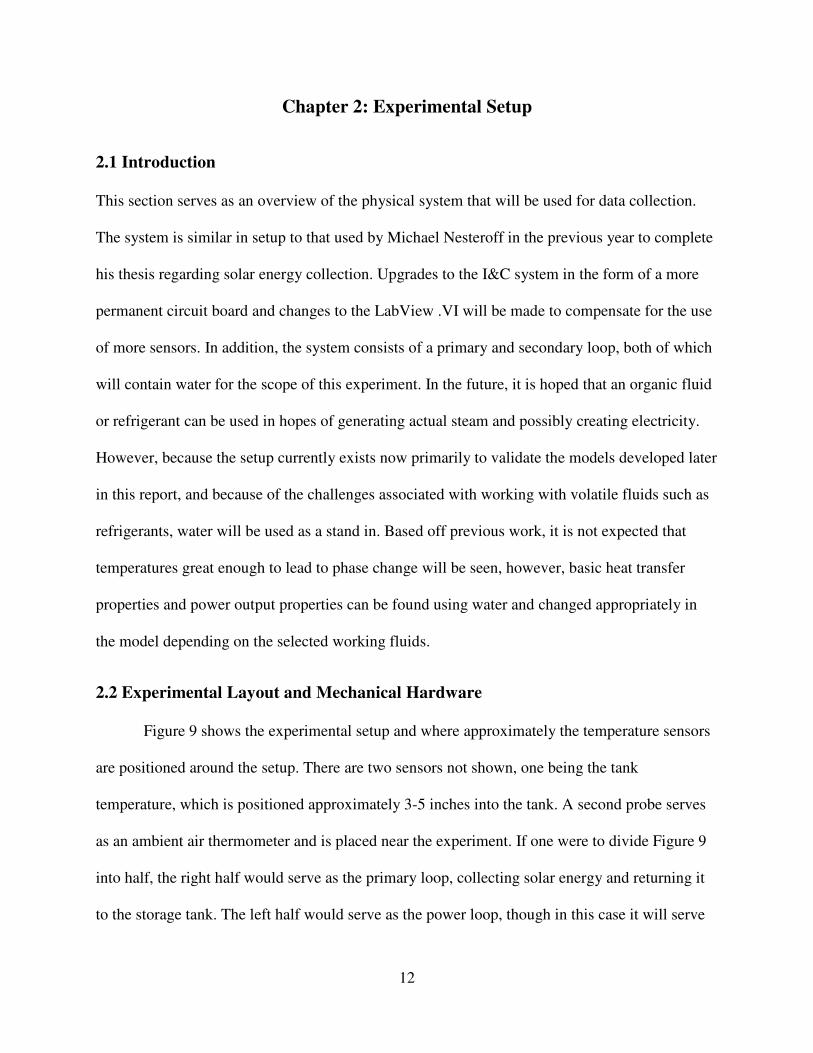
Finally, the Boiler Return Conditions subsystem, Figure 28, gives the temperature and

quality of the return flow to the boiler. It does this by first finding the enthalpy of the returning

flow by subtracting the power out from the enthalpy of the flow initially leaving the boiler, as

shown in Equation 13. It then processes compares the enthalpy to the saturation enthalpies of

liquid and gas, determines the state, and calls the appropriate action block, which use Equations

9 and 10 in reverse to find the temperature and exit quality.

34

'@A��@� '&���A@,AB�� �#�����,�2��� ���# 7� �2����

(13)

Figure 28: Boiler Return Conditions Subsystem

35

Chapter 4: Results and Discussion

For this section, the two portions of this project will be merged. Actual data will be used

to validate the primary loop and to make projections for the secondary loop model. To recap

what data was collected, Table 2 shows what variables were monitored, in what positions, and

Table 2: Data Collection

Temperature 8 Thermistors: 1 on the exit of each manifold(2), one on each

of entrances or exits of the tank (4), 1 for the water in the center

of the tank, and one for ambient temperature

Flow Rate Two flow meters, one for each loop

Solar Insolation Pyranometer normal to the solar collection tubes

how. For this discussion, only the tank temperature, solar insolation, and flow rate on the

primary loop. Poor weather conditions prevented data from being collected this spring and thus

no data exists for the secondary loop. As mentioned above, the purpose of data from the

experiment will be to validate the Simulink model.

4.1 Primary Loop Results and Validation

Though several days of data was collected for the primary loop, most of it involved the testing of

various solar concentrators. These devices negate the efficiency calculation provided by

Fronhaufer and no effort was made to quantize their efficiency. As such, only data from testing

day 1, November 8th

, will be used. Data collection began shortly after sunset and continued

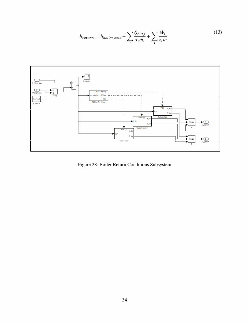
through most of the day, ending just after sunset. Solar insolation for the day is shown below in

Figure 29. As stated before, this is the actual solar insolation coming in normal to the plane of

the tubes. This data was then plugged directly into the primary loop model and the loss

36

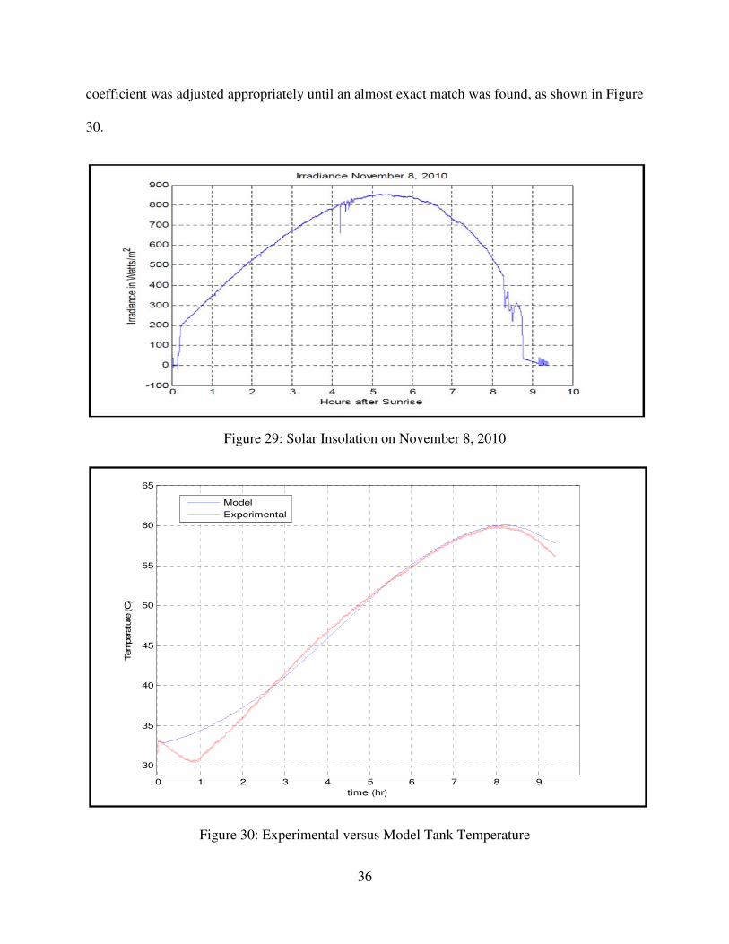
coefficient was adjusted appropriately until an almost exact match was found, as shown in Figure

30.

Figure 29: Solar Insolation on November 8, 2010

Figure 30: Experimental versus Model Tank Temperature

0 1 2 3 4 5 6 7 8 9

30

35

40

45

50

55

60

65

time (hr)

Tem

pera

ture

(C)

Model

Experimental

37

The data shown in Figure 30 is also dependent on flow rate, the mass of water in the tank,

the specific heat of the water, and the ambient temperature. Constants were used for three of

these variables, shown in Table 3. For ambient temperature, this data was recorded, but the

Table 3: Primary Loop Constants

m_dot .34 kg/s

C 4.19 kJ/kg/C

m_tank 150kg

signal quality was poor and several errors made the data nearly unusable. As a result, the

Simulink signal generator was used to closely mimic, though in a more stepped fashion, the

ambient temperature. Finally, the experimentally adjustable loss coefficient was manually

tweaked over several iterations until the results produced those shown in Figure 30. The final

value of the loss coefficient was .0165. It is believed that the initial source of error was a result

of the capacitance of the water and manifolds that were left out overnight in the cold November

air. Though the tank internal temperature was initially around 33C, the water remaining in the

system and the manifolds themselves no doubt cooled down over night, when the testing began,

which was right after sunrise, the low insolation at the time was notquickly overcome this

capacitance. After this test, a final test of the model was run. Though no data exists to give an

idea of energy loss as a result of a thermal load on the secondary side, for modeling purposes, a

step function is added to the tank energy balance. In the case shown in Figure 31, a dummy 500

watt load was applied to the tank at around the 4.2 hours mark. This load was meant to simulate

a load from the secondary loop. Though a load from the secondary loop is likely to be dependent

on the tank temperature and thus more sinusoidal or parabolic in shape, the lack of hard data

38

makes this prediction difficult to do accurately, thus a moderate load was applied just to give an

order of magnitude idea of the temperature loss that may be seen in the tank.

Figure 31: Primary Loop Simulation with 500 Watt Load at 4.2 Hours

4.2 Secondary Side Modeling

As was mentioned previously, no data was able to be collected to validate the secondary

side, therefore all data for the secondary side is based on predictions and guesses based on

experience and realistic expectations. Before continuing with this discussion, a recap of previous

research on the topic of fluid selection is relevant for this section.

0 1 2 3 4 5 6 7 8 9 1032

34

36

38

40

42

44

46

48

50

52

time (hr)

Te

mp

era

ture

(C

)

39

Jake Wither performed a parametric analysis of several refrigerants with low boiling

points that may be ideally suited for this project. His analysis ultimately led to the selection of

R600a as the refrigerant of choice for the secondary side model, though he suggest 3 other fluids

too based on his research, these fluids are shown with some of their properties in Figure 32.

Figure 32: Refrigerant Properties (Wither)

Again, this chart shows that R600a’s boiling points are most in line with temperatures reasonable

for this system. Though not shown, a pressure of 10 bar was used for modeling. The boiling

point of R600a at 10 bar is 66.84 C. though that temperature was never reached under normal

operation conditions, Mike Nesteroff was able to achieve that temperature using simple

reflectors, a more complex reflector may offer an even higher temperature differential for

boiling.

For the actual model simulation, several other variables were selected; more so than on

the primary loop. These constants are shown in Table 4. Figure 25 shows the full T-h diagram

Hot Side

Temperature

Cold Side

Temperature

Environmental

Concerns

Critical

Conditions

40

for n-Pentane, a similar fluid, at 3 and 10 bar. Also important is the input power into the boiler,

which is shown below in Figure 33. This curve is generated from the sin wave function

Table 4: Secondary Side Constants

m_dot .06kg/s

c_vapor 2.232 kJ/kg/C

c_liquid 2.634 kJ/kg/C

h_fg 267.7 kJ/kg

h_f 497.7kJ/kg

h_g 765.4 kJ/kg

h(T=0C, p=10bar) 327.1 kJ/kg

h(p=3bar, x=.9) 670.6 kJ/kg

Figure 33: Power into Boiler

0 100 200 300 400 500 6000.5

1

1.5

2x 10

4

time (s)

Power In

(watts)

41

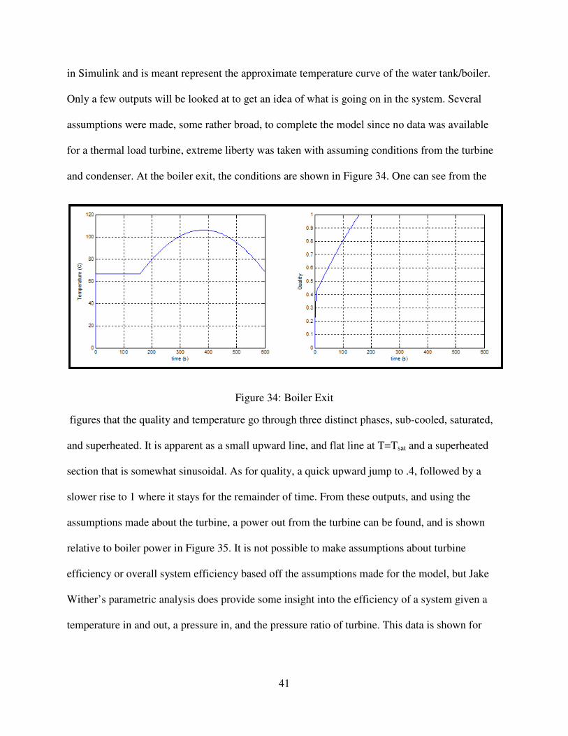
in Simulink and is meant represent the approximate temperature curve of the water tank/boiler.

Only a few outputs will be looked at to get an idea of what is going on in the system. Several

assumptions were made, some rather broad, to complete the model since no data was available

for a thermal load turbine, extreme liberty was taken with assuming conditions from the turbine

and condenser. At the boiler exit, the conditions are shown in Figure 34. One can see from the

Figure 34: Boiler Exit

figures that the quality and temperature go through three distinct phases, sub-cooled, saturated,

and superheated. It is apparent as a small upward line, and flat line at T=Tsat and a superheated

section that is somewhat sinusoidal. As for quality, a quick upward jump to .4, followed by a

slower rise to 1 where it stays for the remainder of time. From these outputs, and using the

assumptions made about the turbine, a power out from the turbine can be found, and is shown

relative to boiler power in Figure 35. It is not possible to make assumptions about turbine

efficiency or overall system efficiency based off the assumptions made for the model, but Jake

Wither’s parametric analysis does provide some insight into the efficiency of a system given a

temperature in and out, a pressure in, and the pressure ratio of turbine. This data is shown for

42

reference sake in Figure 36. This efficiency is based off the returning saturated liquid back to the

boiler.

Figure 35: Turbine Power Out v Boiler Power in

Figure 36: R600a System Efficiency Plot for Varying Expander Inlet Temperatures and Pressure

Ratios, with Inlet Pressure of 10 Bar (Wither)

0 100 200 300 400 500 6000

0.2

0.4

0.6

0.8

1

1.2

1.4

1.6

1.8

2x 10

4

time (s)

Power (w

atts)

Qin

(boiler)

Wout

(turbine)

43

Chapter 5: Conclusion and Recommendations

5.1 Experimental Summary

This report has laid out the experimental setup of a system for collecting data on the

thermal portion of a residential scale solar thermal electrical plant. From a system viability

perspective, the system has shown that it is capable of achieving, if not sustaining, the required

temperatures needed to boil a low pressure refrigerant. With this system viability confirmed,

more testing still remains for the secondary loop to gather data for sufficient modeling. In

addition, work on the low pressure expander continues, and part of this work should include

determining expander efficiency. This efficiency can be used to improve the efficiency of the

parametric models of the fluids and the dynamic modeling of the secondary loop. In fact, it will

be crucial to developing a realistic loop. The radiator in position in the secondary loop of the test

setup is coupled to two DC motors which can be controlled using a PWM duty cycle, just like

the motor, therefore, a wide range of thermal loading opportunities exist for testing. The

aperature surface area can also be increased to bring in more solar energy, and produce higher

temperatures with high flow rates. Overall, the model is very scalable and should serve well into

the future in a variety of tests to determine the overall feasibility of this project.

5.2 Modeling Summary

As was seen, the primary loop of the system has been validated using real data with water

as a working fluid. The option exists to replace water with an oil that may boil at a much higher

temperature, assuming these temperatures can be achieved. It would also be advised to include

temperature capacitance of the manifolds and the water left in them over night. A cold winter

night would drop temperature in the system before a pseudo steady state is reached. The opposite

44

effect may happen on a balmy summer night, with temperature spiking quickly before returning

to a steady climb.

5.3 Recommendations

Data collection remains to be completed on the secondary loop, as an unseasonably cold

and rainy spring made data collection impossible. It is believed that a few days of collection

should allow a relationship between tank temperature and secondary loop return temperature to

equate to a total power out of the tank and into the secondary loop. This would essentially allow

the two loops to be coupled into a single model. Finally, as was mentioned above, work can be

done to improve the secondary loop. There are three key points to be improved upon.

1. Development of turbine efficiency and work equations to accurately model whatever

form of expander is ultimately used.

2. Development of equations of more accurate assessment of the energy out of the

condenser/radiator setup.

3. Addition of losses to the secondary loop, similar to that of the primary loop.

If these three points can be adequately addressed, complete simulation of the system under any

conceived conditions should be possible.

45

Bibliography

Arduino. 12 April 2011 <arduino.cc>.

Arenberg, Amy Lo and Jonathan. New architecture for space telescopes uses Fresnel lenses. 9

August 2006. <http://spie.org/x8645.xml?ArticleID=x8645>.

Baetz, Juergen. Bloomberg.com. 20 January 2011. <http://www.bloomberg.com/news/2011-01-

20/germany-to-trim-solar-power-subsidies.html>.

Department of Energy. <doe.gov>.

EIA. Domestic Energy Consumption. <http://www.eia.gov/forecasts/aeo/early_fuel.cfm>.

Energiesystem, Fraunhofer Institut Solare. Collector test according to EN 12975-1,2:2006.

Product Report. Freiburg, 2008.

"E-Solar Inc." <http://www.esolar.com/esolar_brochure.pdf>.

Laherrere, J. Estimate of Oil Reserves. Laxenburg: EMF/IEA/IEW, 2001.

Mims, Christopher. Germany’s solar panels produce more power than Japan’s entire Fukushima

complex. 22 Mar 2011. <http://www.grist.org/list/2011-03-22-germanys-solar-panels-produce-

more-power-than-japans-entire-fuku>.

Nesteroff, Mike. Solar Collection of Evacuated Tubes in a Residential Electrical Power System.

Thesis. Columbus, 2010.

46

Newscientist. 27 October 2010. <http://www.newscientist.com/article/mg20827842.800-solar-

power-could-crash-germanys-grid.html>.

NREL. National Renewable Energy Lab, Wind Systems Integration . 24 August 2010.

<http://www.nrel.gov/wind/systemsintegration/images/home_usmap.jpg>.

Quaschning, V. 2010. Solar Thermal Power Plants. <http://www.volker-

quaschning.de/articles/fundamentals2/index.php>.

Wither, Jake. Numerical Analysis of Residential Electricity Generation. Thesis. Columbus, 2010.