doi:10.1152/jn.00684.2004 94:1443-1458, 2005. First published 13 April 2005;J NeurophysiolHochner and Tamar FlashYoram Yekutieli, Roni Sagiv-Zohar, Ranit Aharonov, Yaakov Engel, Binyaminof the Octopus Reaching MovementDynamic Model of the Octopus Arm. I. Biomechanics

You might find this additional info useful...

28 articles, 11 of which can be accessed free at:This article cites http://jn.physiology.org/content/94/2/1443.full.html#ref-list-1

5 other HighWire hosted articlesThis article has been cited by

  [PDF] [Full Text]

, November 1, 2005; 208 (21): iv.J Exp BiolLaura BlackburnAGILE ANIMALS 

[PDF] [Full Text] [Abstract], October 1, 2006; 209 (19): 3697-3707.J Exp Biol

Christine L. Huffardbetween primary and secondary defenses

(Cephalopoda: Octopodidae): walking the lineAbdopus aculeatusLocomotion by  

[PDF] [Full Text] [Abstract], September 1, 2007; 98 (3): 1775-1790.J Neurophysiol

Yoram Yekutieli, Rea Mitelman, Binyamin Hochner and Tamar FlashAnalyzing Octopus Movements Using Three-Dimensional Reconstruction 

[PDF] [Full Text] [Abstract], December 1, 2007; 210 (23): 4069-4082.J Exp Biol

Richard J. Gilbert, Vitaly J. Napadow, Terry A. Gaige and Van J. WedeenAnatomical basis of lingual hydrostatic deformation 

[PDF] [Full Text] [Abstract], November , 2010; 109 (5): 1500-1514.J Appl Physiol

Richard J. GilbertSrboljub M. Mijailovich, Boban Stojanovic, Milos Kojic, Alvin Liang, Van J. Wedeen andmechanics of mesoscale myofiber tracts obtained by MRIDerivation of a finite-element model of lingual deformation during swallowing from the

including high resolution figures, can be found at:Updated information and services http://jn.physiology.org/content/94/2/1443.full.html

can be found at:Journal of Neurophysiologyabout Additional material and information http://www.the-aps.org/publications/jn

This infomation is current as of October 6, 2011. 

American Physiological Society. ISSN: 0022-3077, ESSN: 1522-1598. Visit our website at http://www.the-aps.org/.(monthly) by the American Physiological Society, 9650 Rockville Pike, Bethesda MD 20814-3991. Copyright © 2005 by the

publishes original articles on the function of the nervous system. It is published 12 times a yearJournal of Neurophysiology

on October 6, 2011

jn.physiology.orgD

ownloaded from

Dynamic Model of the Octopus Arm. I. Biomechanics of the OctopusReaching Movement

Yoram Yekutieli,1,2,* Roni Sagiv-Zohar,1,* Ranit Aharonov,2 Yaakov Engel,2 Binyamin Hochner,1,2

and Tamar Flash3

1Department of Neurobiology and 2Interdisciplinary Center for Neural Computation, Hebrew University, Jerusalem; and 3Department ofComputer Science and Applied Mathematics, Weizmann Institute of Science, Rehovot, Israel

Submitted 6 July 2004; accepted in final form 2 March 2005

Yekutieli, Yoram, Roni Sagiv-Zohar, Ranit Aharonov, YaakovEngel, Binyamin Hochner, and Tamar Flash. Dynamic model ofthe octopus arm. I. Biomechanics of the octopus reaching movement.J Neurophysiol 94: 1443–1458, 2005. First published April 13, 2005;doi:10.1152/jn.00684.2004. The octopus arm requires special motorcontrol schemes because it consists almost entirely of muscles andlacks a rigid skeletal support. Here we present a 2D dynamic model ofthe octopus arm to explore possible strategies of movement control inthis muscular hydrostat. The arm is modeled as a multisegmentstructure, each segment containing longitudinal and transverse mus-cles and maintaining a constant volume, a prominent feature ofmuscular hydrostats. The input to the model is the degree of activationof each of its muscles. The model includes the external forces ofgravity, buoyancy, and water drag forces (experimentally estimatedhere). It also includes the internal forces generated by the arm musclesand the forces responsible for maintaining a constant volume. Usingthis dynamic model to investigate the octopus reaching movement andto explore the mechanisms of bend propagation that characterize thismovement, we found the following. 1) A simple command producinga wave of muscle activation moving at a constant velocity is sufficientto replicate the natural reaching movements with similar kinematicfeatures. 2) The biomechanical mechanism that produces the reachingmovement is a stiffening wave of muscle contraction that pushes abend forward along the arm. 3) The perpendicular drag coefficient foran octopus arm is nearly 50 times larger than the tangential dragcoefficient. During a reaching movement, only a small portion of thearm is oriented perpendicular to the direction of movement, thusminimizing the drag force.

I N T R O D U C T I O N

The biomechanical principles of movement generation differin animals with and without a rigid skeleton. The latter possessa hydrostatic skeleton, consisting mainly of muscles and fluid,which because they are incompressible, support the flexiblebody. Hydrostatic skeletons are generally of 2 types. In mus-cular hydrostats, muscles and other tissues form a solid struc-ture without a separate enclosed fluid volume (e.g., cephalopodtentacles, elephant trunk, vertebrate tongue; Kier and Smith1985). In a second type of hydrostatic skeleton, musclescompose a body wall that surrounds a fluid-filled cavity (e.g.,sea anemones and worms, Kier 1992).

All muscular hydrostats consist of closely packed arrays ofmuscle fibers organized in 3 main directions (Kier and Smith1985): parallel, perpendicular, and helical or oblique to the

long axis. The major feature of muscular hydrostats is that theymaintain a constant volume (Kier and Smith 1985). Thisconstraint allows forces to be transferred between the longitu-dinal and the transverse directions. All motion in a muscularhydrostat is based on combinations of 4 elementary movementsthat can occur at any location: elongation, shortening, torsion,and bending (Kier and Smith 1985). Muscular hydrostats thushave an exciting and unique property: the muscles not onlygenerate the forces required to implement movements, but alsoprovide the skeletal support, i.e., the muscular system canfunction as a dynamic skeleton. This allows smooth changes ofshape, resulting in a potentially vast repertoire of movements.

While an articulated arm has a limited number of degrees offreedom (DOFs), the octopus arm has virtually an infinitenumber of degrees of freedom and thus poses a considerablechallenge from the control perspective.

The uniqueness of this system raises fundamental questions:What constraints does the mechanical structure of the muscularhydrostat structure impose on the motor control system? Howdoes the motor control system select a specific movement froman apparently infinite number of available possibilities? Whatdoes the movement repertoire of the octopus arm teach usabout evolutionary and optimization processes and the con-straints that have shaped the octopus motor control system?How does the nervous system control and coordinate themuscles?

Understanding the principles that govern the motion of thisarm is not only interesting from the biological standpoint but isalso important for robotics engineering. Researchers in thisfield face similarly complex problems when designing controlsystems for flexible robotic arms with a large number of DOFs(e.g., Chirikjian and Burdick 1994; Takanashi et al. 1993;Walker 2000).

Reaching movement

The octopus uses a limited number of stereotypical motionpatterns to reach out to catch and inspect an object (Gutfreundet al. 1996, 1998). A bend is created, usually near the base ofthe arm (but it can be created almost anywhere along the arm),and is propagated along the arm toward the tip. The armsegment proximal to the bend is maintained relatively straightand the bend is always curved dorsally (Fig. 6A). The path ofthis bend is confined to a plane and the bend propagates

* Y. Yekutieli and R. Sagiv-Zohar contributed equally to this work.Address for reprint requests and other correspondence: T. Flash, The Faculty

of Mathematics and Computer Science, The Weizmann Institute of Science,POB 26, Rehovot 76100, Israel (E-mail tamar.flash@weizmann.ac.il).

The costs of publication of this article were defrayed in part by the paymentof page charges. The article must therefore be hereby marked “advertisement”in accordance with 18 U.S.C. Section 1734 solely to indicate this fact.

J Neurophysiol 94: 1443–1458, 2005.First published April 13, 2005; doi:10.1152/jn.00684.2004.

14430022-3077/05 $8.00 Copyright © 2005 The American Physiological Societywww.jn.org

on October 6, 2011

jn.physiology.orgD

ownloaded from

according to an invariant basic velocity profile. Gutfreund et al.(1996) proposed that this mode of reaching solves the problemof multiple DOFs by reducing their potentially large number toa very small number of control parameters that shape themovement—one DOF for the motion of the bend along the armand 2 additional DOFs for the orientation of the base of the armin space. Sumbre et al. (2001) suggested that the brain issuescommands to orient the arm direction and set the extensionparameters, whereas the details for muscle activation are rep-resented and carried out within the neuromuscular system ofthe arm itself.

Bending results from a selective contraction of longitudinalmuscles on one side of the arm together with the contraction oftransverse muscles to resist shortening (Kier 1992; Kier andSmith 1985). The pattern of muscle activation that created thebend can then be propagated along the arm creating an exten-sion movement. Gutfreund et al. (1998) proposed a differentmechanism for bend propagation—a stiffening wave caused bya symmetrical muscle activation pattern that propagates alongthe arm and propels an existing bend. The model of the octopusarm that is presented here was developed to test the plausibilityof the stiffening wave hypothesis and how such a wave can becontrolled to produce extension movements.

Modeling muscular hydrostats

We do not fully understand the constraints imposed by thebiomechanics of muscular hydrostats on their control systems,nor the strategies these control systems adopt. Because thesecannot be studied only by an experimental approach, severalmathematical models have been developed to characterizemuscular hydrostats. Most of these muscular hydrostat modelsare not sufficiently general to describe the motion of theoctopus arm for one or more of the following reasons.

1) The models are static or quasi-static, i.e., they do notdescribe the full dynamics of motion: Wadepuhl and Beyn(1989) developed a quasi-static model of wormlike forms;Skierczynski et al. (1996) and Kristan et al. (2000) developeda quasi-static model of the hydrostatic skeleton of the medic-inal leech; and Wilson et al. (1991) gave a static continuummodel of the elephant trunk. Related to these models arekinematic models; Drushel et al. (1998) constructed 2 kine-matic models of the buccal mass of Aplysia californica. (SeeDrushel et al. 2002 and Neustadter et al. 2002 for the devel-opment of these models.)

2) The models are restricted to describe specific movementscharacterized by a low number of DOFs. Van Leeuwen andKier (1997) developed a dynamical model of the squid tenta-cles capable of producing fast elongation extension move-ments. This model can describe only the forward extension ofthe tentacle.

3) The models cannot account for all feasible motions (e.g.,they assume some constraints on the shape of the structure).Chiel et al. (1992) produced a quantitative model of thereptilian tongue, but they neglected mass and inertial forces,which are likely to be small compared to the muscle forcesinvolved in the movements they modeled.

4) The models do not consider external forces like gravityor water drag forces, which need to be considered whenmodeling unconstrained movements of the octopus arm (e.g.,Alscher and Beyn 1998; Wadepuhl and Beyn 1989).

5) The models do not incorporate the constant volumeconstraint. For example, Jordan (1996) developed a dynamicalmodel of the leech that couples internal factors (masses,muscle mechanics, soft tissue mechanics, and muscle activa-tion patterns) and external factors (water hydrodynamics) topredict the swimming behavior. This model used a rigidendoskeleton as a first approximation to the hydrostaticskeleton.

Some of these problems are remedied by our dynamic modelof the octopus arm, based on physiological and kinematicstudies. This model is currently essentially 2-dimensional (2D),although it allows natural extension to 3 dimensions.

Here we show that the physics of the arm and its interactionwith water play a significant role in shaping the arm’s move-ments. We show that an extension movement similar to thenatural reaching movement can be produced by a simple neuralcommand propagating along the arm. This produces a wave ofmuscle contraction that travels along the arm, causing it toextend. In paper II, the second part of this z-part series(Yekutieli et al. 2005), we investigate the control of reachingmovements, focusing on the properties of the command thatcreates the wave of muscle contraction. We show a relationshipbetween the amplitude and timing of this command, whichmay be used by the motor control system to choose theminimal forces needed to extend an arm according to a desiredkinematic plan. Our model predicts the possibility of usinghigher forces to resist external perturbations while keeping thesame kinematics. This prediction suggests that the octopus maybe able to independently control 2 major aspects of armextension: the kinematics of the movement and its resistance toperturbations.

A preliminary report on our work was presented in Aha-ronov et al. (1997).

T H E M E C H A N I C A L M O D E L — A N O V E R V I E W

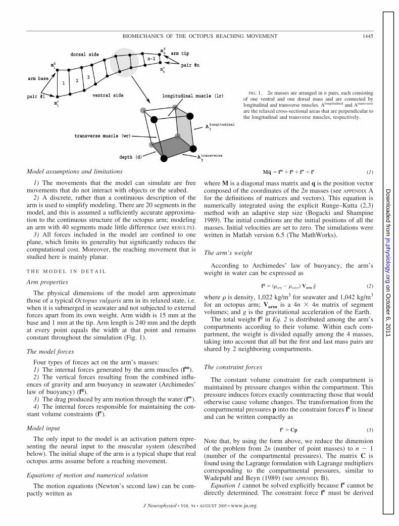
The arm is modeled as a 2D array of point masses andsprings. All the arm’s mass is concentrated in discrete pointmasses connected by massless idealized muscles that are mod-eled as damped (linear or nonlinear) springs (Fig. 1). The 2nmasses are arranged in n pairs, each consisting of one ventraland one dorsal mass. The longitudinal muscles and the trans-verse muscles connect the masses. Through this arrangement,every 2 adjacent pairs of masses and their correspondingmuscles enclose a quadrilateral compartment. These (n � 1)compartments play a crucial role in the model because theconstant volume constraint is enforced locally in each of thecompartments. [See Fig. 10 in Kier (1988) for the arrangementof the musculature of the octopus arm.]

Our model is 2D in the sense that all force vectors lie withinthe x–y plane, where �y is the direction of gravity; thus thearm’s motion is constrained to be planar. The following nota-tions are used throughout:

x a scalarr� a vector in �2 or �3 of a physical quantity like velocityr a vector in �m, m � 3x� a scalar average valueX a matrixxi, xij elements of a vector and matrix, respectivelyx, x time derivatives of x and x, respectively

1444 YEKUTIELI ET AL.

J Neurophysiol • VOL 94 • AUGUST 2005 • www.jn.org

on October 6, 2011

jn.physiology.orgD

ownloaded from

Model assumptions and limitations

1) The movements that the model can simulate are freemovements that do not interact with objects or the seabed.

2) A discrete, rather than a continuous description of thearm is used to simplify modeling. There are 20 segments in themodel, and this is assumed a sufficiently accurate approxima-tion to the continuous structure of the octopus arm; modelingan arm with 40 segments made little difference (see RESULTS).

3) All forces included in the model are confined to oneplane, which limits its generality but significantly reduces thecomputational cost. Moreover, the reaching movement that isstudied here is mainly planar.

T H E M O D E L I N D E T A I L

Arm properties

The physical dimensions of the model arm approximatethose of a typical Octopus vulgaris arm in its relaxed state, i.e.when it is submerged in seawater and not subjected to externalforces apart from its own weight. Arm width is 15 mm at thebase and 1 mm at the tip. Arm length is 240 mm and the depthat every point equals the width at that point and remainsconstant throughout the simulation (Fig. 1).

The model forces

Four types of forces act on the arm’s masses:1) The internal forces generated by the arm muscles (fm).2) The vertical forces resulting from the combined influ-

ences of gravity and arm buoyancy in seawater (Archimedes’law of buoyancy) (fg).

3) The drag produced by arm motion through the water (fw).4) The internal forces responsible for maintaining the con-

stant volume constraints (fc).

Model input

The only input to the model is an activation pattern repre-senting the neural input to the muscular system (describedbelow). The initial shape of the arm is a typical shape that realoctopus arms assume before a reaching movement.

Equations of motion and numerical solution

The motion equations (Newton’s second law) can be com-pactly written as

Mq � fm � fg � fw � fc (1)

where M is a diagonal mass matrix and q is the position vectorcomposed of the coordinates of the 2n masses (see APPENDIX Afor the definitions of matrices and vectors). This equation isnumerically integrated using the explicit Runge–Kutta (2,3)method with an adaptive step size (Bogacki and Shampine1989). The initial conditions are the initial positions of all themasses. Initial velocities are set to zero. The simulations werewritten in Matlab version 6.5 (The MathWorks).

The arm’s weight

According to Archimedes’ law of buoyancy, the arm’sweight in water can be expressed as

fg � ��arm � �water� Varm g� (2)

where � is density, 1,022 kg/m3 for seawater and 1,042 kg/m3

for an octopus arm; Varm is a 4n � 4n matrix of segmentvolumes; and g is the gravitational acceleration of the Earth.

The total weight fg in Eq. 2 is distributed among the arm’scompartments according to their volume. Within each com-partment, the weight is divided equally among the 4 masses,taking into account that all but the first and last mass pairs areshared by 2 neighboring compartments.

The constraint forces

The constant volume constraint for each compartment ismaintained by pressure changes within the compartment. Thispressure induces forces exactly counteracting those that wouldotherwise cause volume changes. The transformation from thecompartmental pressures p into the constraint forces fc is linearand can be written compactly as

fc � Cp (3)

Note that, by using the form above, we reduce the dimensionof the problem from 2n (number of point masses) to n � 1(number of the compartmental pressures). The matrix C isfound using the Lagrange formulation with Lagrange multiplierscorresponding to the compartmental pressures, similar toWadepuhl and Beyn (1989) (see APPENDIX B).

Equation 1 cannot be solved explicitly because fc cannot bedirectly determined. The constraint force fc must be derived

FIG. 1. 2n masses are arranged in n pairs, each consistingof one ventral and one dorsal mass and are connected bylongitudinal and transverse muscles. Alongitudinal and Atransverse

are the relaxed cross-sectional areas that are perpendicular tothe longitudinal and transverse muscles, respectively.

1445BIOMECHANICS OF THE OCTOPUS REACHING MOVEMENT

J Neurophysiol • VOL 94 • AUGUST 2005 • www.jn.org

on October 6, 2011

jn.physiology.orgD

ownloaded from

indirectly from the constant volume constraints (see APPENDIX

B). The result of the derivation is the pressure vector p

p � �GM�1C��1�� � GM�1�fm � fg � fw�� (4)

(See APPENDIX B for the definition and derivation of the matrixG and the vector �.)

Once the compartmental pressures p are known, they can belinearly transformed into fc (Eq. 3). All forces are now ex-pressed explicitly and the equations of motion can be solved

q � M�1�fm � fg � fw � fc� (5)

The drag forces

A body moving through fluid is subjected to drag forces thatincrease with the relative velocity of the body. This depen-dency of drag force on velocity is rather complex because it iscomposed of a direct dependency on the squared velocity, andan indirect effect through the Reynolds number,1 which itselfdepends on velocity. The characteristic velocities of octopusarms during reaching movements in seawater lie in the range of20–60 cm/s (Gutfreund et al. 1996). The Reynolds number ofan octopus arm for these conditions is �3000 (see details inCALCULATIONS AND SIMPLIFICATIONS below). A value of Re be-tween 50 and 200,000 indicates a moderately turbulent flow.

When the arm moves in water, each of the segments moveswith some velocity v that can be decomposed into 2 compo-nents: vper in the direction perpendicular to the long axis of thesegment and vtan in the direction tangential to the long axis.Similarly, the water drag forces acting on the segment can bedecomposed into a perpendicular component dper and a tan-gential component dtan.

Both the perpendicular and the tangential components of thedrag forces are calculated for each segment and then decom-posed into their x and y components. Following Newton’ssecond law and the dimensional analysis technique,2 the twodrag components in steady flow3 are (Vogel 1981)

�d� per� �1

2�waterpacper�v�per�2 (6)

�d� tan� �1

2�waterSactan�v�tan�2 (7)

where Pa is the projected area of the segment in the planeperpendicular to the direction of v�per and Sa is the surface areaof the segment. The components of the segment’s velocity inthe perpendicular and tangential directions are v�per and v�tan,respectively. The coefficients cper and ctan express the perpen-

dicular and tangential drag coefficients, respectively, which arefunctions of Reynolds number as follows

cper � f �Re �v�per��

ctan � g�Re �v�tan��

The functions f and g are of the form u1 � u2(Re)u3, where u1,u2, and u3 are scalars (Vogel 1981).

A biologically inspired model for swimming in the chaeto-gnath Sagitta elegans (Jordan 1992) was based on the dragforce equations (Eq. 6 and 7). It used a perpendicular dragcoefficient (cper) from curves fitted for cylinders in cross flow,4

and a tangential drag coefficient (ctan) from curves fitted for flatplates in streamwise flow.5 The functions expressing the per-pendicular and tangential drag coefficients were taken fromVogel (1981) and White (1974) and were expressed as follows

cper � 1 � 10�Reper��2/3

ctan � 0.64�Retan��1/2

where Reper, the Reynolds number for the perpendicular direc-tion, is (2rv)/�, where r is the cylinder radius and � is thekinematic viscosity. Reynolds number for the tangential direc-tion Retan is (xv)/�, where x is the cumulative cylinder’s length.

Experimental estimation of the drag forces

We did not use the above tangential and perpendicular dragcoefficients (Jordan 1992) but instead experimentally estimatedthe drag forces for the following reasons: 1) The drag coeffi-cients depend strongly on the structure and surface propertiesof the moving body. The shape of the octopus arm is verycomplex, but Jordan’s values were obtained for idealizedshapes. 2) It is essential to use as accurate values as possiblebecause we found that the behavior produced by the model issensitive to changes in the values of the drag coefficients(especially the tangential one; see below in RESULTS).

An experiment was used to evaluate the 2 components of thedrag force, dper and dtan. First we calculated the real projectedarea Pa and sectional area Sa. We then used Eq. 6 and 7 toobtain the experimental drag coefficients cper and ctan. Thesevalues were inserted into the model as described next.

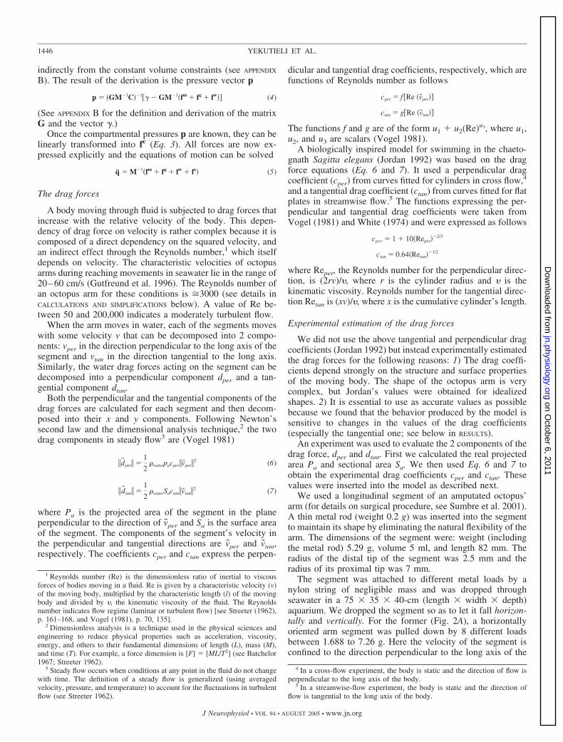
We used a longitudinal segment of an amputated octopus’arm (for details on surgical procedure, see Sumbre et al. 2001).A thin metal rod (weight 0.2 g) was inserted into the segmentto maintain its shape by eliminating the natural flexibility of thearm. The dimensions of the segment were: weight (includingthe metal rod) 5.29 g, volume 5 ml, and length 82 mm. Theradius of the distal tip of the segment was 2.5 mm and theradius of its proximal tip was 7 mm.

The segment was attached to different metal loads by anylon string of negligible mass and was dropped throughseawater in a 75 � 35 � 40-cm (length � width � depth)aquarium. We dropped the segment so as to let it fall horizon-tally and vertically. For the former (Fig. 2A), a horizontallyoriented arm segment was pulled down by 8 different loadsbetween 1.688 to 7.26 g. Here the velocity of the segment isconfined to the direction perpendicular to the long axis of the

1 Reynolds number (Re) is the dimensionless ratio of inertial to viscousforces of bodies moving in a fluid. Re is given by a characteristic velocity (v)of the moving body, multiplied by the characteristic length (l) of the movingbody and divided by �, the kinematic viscosity of the fluid. The Reynoldsnumber indicates flow regime (laminar or turbulent flow) [see Streeter (1962),p. 161–168, and Vogel (1981), p. 70, 135].

2 Dimensionless analysis is a technique used in the physical sciences andengineering to reduce physical properties such as acceleration, viscosity,energy, and others to their fundamental dimensions of length (L), mass (M),and time (T). For example, a force dimension is [F] [ML/T2] (see Batchelor1967; Streeter 1962).

3 Steady flow occurs when conditions at any point in the fluid do not changewith time. The definition of a steady flow is generalized (using averagedvelocity, pressure, and temperature) to account for the fluctuations in turbulentflow (see Streeter 1962).

4 In a cross-flow experiment, the body is static and the direction of flow isperpendicular to the long axis of the body.

5 In a streamwise-flow experiment, the body is static and the direction offlow is tangential to the long axis of the body.

1446 YEKUTIELI ET AL.

J Neurophysiol • VOL 94 • AUGUST 2005 • www.jn.org

on October 6, 2011

jn.physiology.orgD

ownloaded from

segment. In the vertical fall (Fig. 2B), a vertically oriented armsegment was pulled down by 13 different loads between 0.145to 0.947 g. The segment’s velocity was confined to the direc-tion tangential to the long axis of the segment. All falls wererepeated 4–6 times for each load. Images of the falling armsegment were recorded by a PAL S-VHS video camera with 40ms between adjacent frames.

CALCULATIONS AND SIMPLIFICATIONS. When the segment isdropped, it accelerates until its velocity levels off at someconstant value, i.e., no net force acts on the segment (byNewton’s second law ¥i f�i � 0 where f� are force vectors). Inour experiment, the relevant forces acting on the segment wereconfined to the vertical direction.

The force equations are

dtan � fAse � fAlo � Wse � Wlo � 0 (8)

dper � fAse � fAlo � Wse � Wlo � 0 (9)

where fAse Vse�g� is Archimedes’ force acting on the segmentand fAlo Vlo�g� is Archimedes’ force acting on the load. Thevolumes of the segment and the load are Vse and Vlo, respec-tively, and the weight of the segment and the load are Wse andWlo.

In Eq. 8 and 9 all forces except the drag forces are known orcan be easily determined, so the extraction of the drag forces istrivial.

To estimate the projected area p and the surface area s, weused a truncated cone as a simplification for the more complexstructure of the octopus arm. The projected area Pa is 2r�l,

where r� is the mean segment radius of the arm and l is thesegment length. The sectional surface area Sa is 2�r�l.

For the perpendicular component Re 2r�v�per /�. For thetangential component Re lv�tan/�, where l is the segmentlength, v� is the segment average velocity, r� is the segmentaverage radius, and � is the kinematic viscosity (� 1 � 10�6

m2/s).

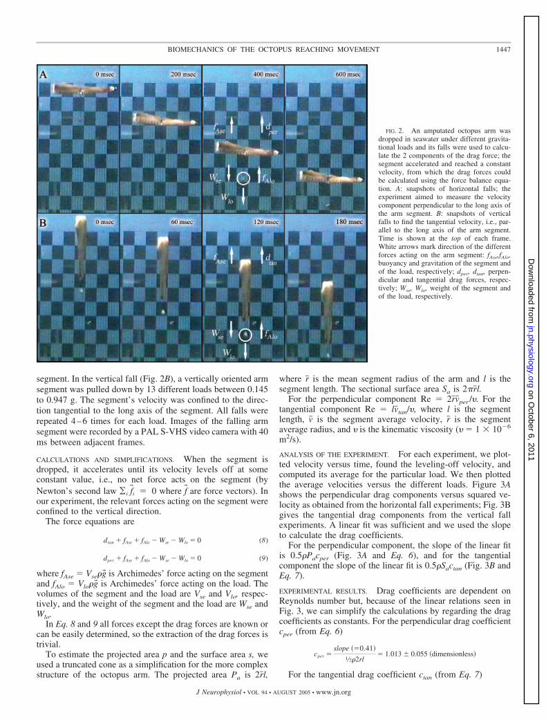
ANALYSIS OF THE EXPERIMENT. For each experiment, we plot-ted velocity versus time, found the leveling-off velocity, andcomputed its average for the particular load. We then plottedthe average velocities versus the different loads. Figure 3Ashows the perpendicular drag components versus squared ve-locity as obtained from the horizontal fall experiments; Fig. 3Bgives the tangential drag components from the vertical fallexperiments. A linear fit was sufficient and we used the slopeto calculate the drag coefficients.

For the perpendicular component, the slope of the linear fitis 0.5�Pacper (Fig. 3A and Eq. 6), and for the tangentialcomponent the slope of the linear fit is 0.5�Sactan (Fig. 3B andEq. 7).

EXPERIMENTAL RESULTS. Drag coefficients are dependent onReynolds number but, because of the linear relations seen inFig. 3, we can simplify the calculations by regarding the dragcoefficients as constants. For the perpendicular drag coefficientcper (from Eq. 6)

cper �slope �0.41�

1⁄2�2rl� 1.013 � 0.055 �dimensionless�

For the tangential drag coefficient ctan (from Eq. 7)

FIG. 2. An amputated octopus arm wasdropped in seawater under different gravita-tional loads and its falls were used to calcu-late the 2 components of the drag force; thesegment accelerated and reached a constantvelocity, from which the drag forces couldbe calculated using the force balance equa-tion. A: snapshots of horizontal falls; theexperiment aimed to measure the velocitycomponent perpendicular to the long axis ofthe arm segment. B: snapshots of verticalfalls to find the tangential velocity, i.e., par-allel to the long axis of the arm segment.Time is shown at the top of each frame.White arrows mark direction of the differentforces acting on the arm segment: fAse,fAlo,buoyancy and gravitation of the segment andof the load, respectively; dper, dtan, perpen-dicular and tangential drag forces, respec-tively; Wse, Wlo, weight of the segment andof the load, respectively.

1447BIOMECHANICS OF THE OCTOPUS REACHING MOVEMENT

J Neurophysiol • VOL 94 • AUGUST 2005 • www.jn.org

on October 6, 2011

jn.physiology.orgD

ownloaded from

ctan �slope (0.033)

1⁄2�2�rl� 0.0256 � 0.0017 �dimensionless�

Note that the perpendicular drag coefficient is nearly 50-foldlarger than the tangential drag coefficient. This difference maybe one of the factors that shaped the octopus reaching move-ment such that only a small portion of the arm is orientedperpendicular to the direction of movement, thus minimizingthe drag force (see DISCUSSION).

Muscle forces

We used 2 types of muscle models.1) A nonlinear model similar to the models described by

Van Leeuwen and Kier (1997) and Zajac (1989). It includesnonlinear force–length and force–velocity relations.

2) A linear damped spring model (similar to the model ofEkeberg 1993).

Most of our work used the nonlinear muscle model. This iscompared with the linear model below.

We assume that the arm’s muscle fibers are homogeneousand evenly distributed throughout the arm and that all muscleshave similar functional properties (Matzner et al. 2000). Thevarious parameters of each muscle model are scaled for thedimensions of the different muscles according to the dimen-sions of a real octopus arm in a relaxed state.

For simplicity, we present only the magnitude of the forceand not its direction, but all real calculations are vectorial,taking the direction into account.

The nonlinear muscle model

Every muscle in the model exerts the following force

f�t� � A�a�t�Fa�l�t�

l0m �Fv� v

vmax�� Fp�l�t�

l0m �� (10)

where A is the cross-sectional area of the muscle, a � [0, 1] isa dimensionless activation function, l(t) is muscle length, andl0m is the specific length of the muscle at which active muscle

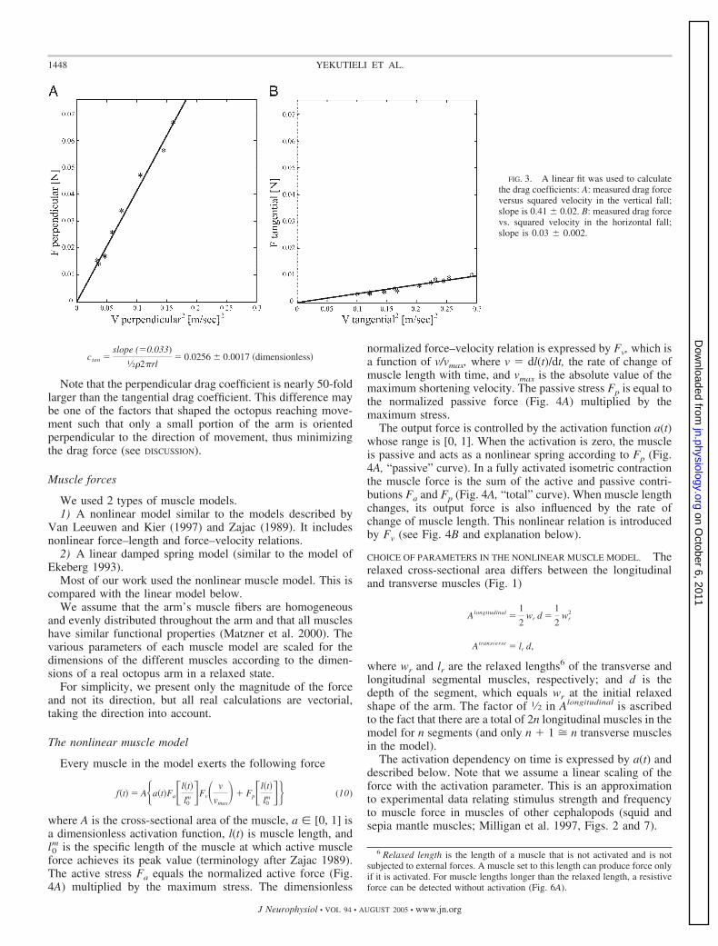
force achieves its peak value (terminology after Zajac 1989).The active stress Fa equals the normalized active force (Fig.4A) multiplied by the maximum stress. The dimensionless

normalized force–velocity relation is expressed by Fv, which isa function of v/vmax, where v dl(t)/dt, the rate of change ofmuscle length with time, and vmax is the absolute value of themaximum shortening velocity. The passive stress Fp is equal tothe normalized passive force (Fig. 4A) multiplied by themaximum stress.

The output force is controlled by the activation function a(t)whose range is [0, 1]. When the activation is zero, the muscleis passive and acts as a nonlinear spring according to Fp (Fig.4A, “passive” curve). In a fully activated isometric contractionthe muscle force is the sum of the active and passive contri-butions Fa and Fp (Fig. 4A, “total” curve). When muscle lengthchanges, its output force is also influenced by the rate ofchange of muscle length. This nonlinear relation is introducedby Fv (see Fig. 4B and explanation below).

CHOICE OF PARAMETERS IN THE NONLINEAR MUSCLE MODEL. Therelaxed cross-sectional area differs between the longitudinaland transverse muscles (Fig. 1)

Alongitudinal �1

2wr d �

1

2wr

2

Atransverse � lr d,

where wr and lr are the relaxed lengths6 of the transverse andlongitudinal segmental muscles, respectively; and d is thedepth of the segment, which equals wr at the initial relaxedshape of the arm. The factor of 1⁄2 in Alongitudinal is ascribedto the fact that there are a total of 2n longitudinal muscles in themodel for n segments (and only n � 1 � n transverse musclesin the model).

The activation dependency on time is expressed by a(t) anddescribed below. Note that we assume a linear scaling of theforce with the activation parameter. This is an approximationto experimental data relating stimulus strength and frequencyto muscle force in muscles of other cephalopods (squid andsepia mantle muscles; Milligan et al. 1997, Figs. 2 and 7).

6 Relaxed length is the length of a muscle that is not activated and is notsubjected to external forces. A muscle set to this length can produce force onlyif it is activated. For muscle lengths longer than the relaxed length, a resistiveforce can be detected without activation (Fig. 6A).

FIG. 3. A linear fit was used to calculatethe drag coefficients: A: measured drag forceversus squared velocity in the vertical fall;slope is 0.41 0.02. B: measured drag forcevs. squared velocity in the horizontal fall;slope is 0.03 0.002.

1448 YEKUTIELI ET AL.

J Neurophysiol • VOL 94 • AUGUST 2005 • www.jn.org

on October 6, 2011

jn.physiology.orgD

ownloaded from

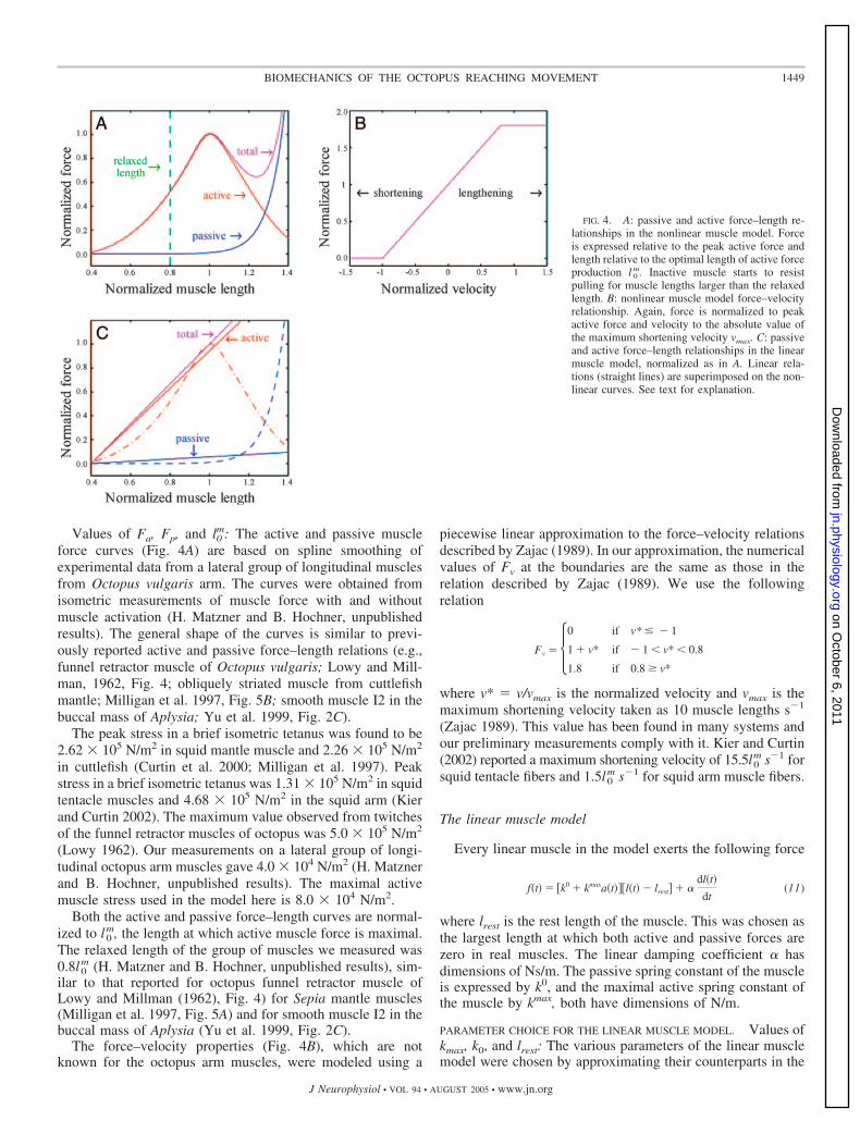
Values of Fa, Fp, and l0m: The active and passive muscle

force curves (Fig. 4A) are based on spline smoothing ofexperimental data from a lateral group of longitudinal musclesfrom Octopus vulgaris arm. The curves were obtained fromisometric measurements of muscle force with and withoutmuscle activation (H. Matzner and B. Hochner, unpublishedresults). The general shape of the curves is similar to previ-ously reported active and passive force–length relations (e.g.,funnel retractor muscle of Octopus vulgaris; Lowy and Mill-man, 1962, Fig. 4; obliquely striated muscle from cuttlefishmantle; Milligan et al. 1997, Fig. 5B; smooth muscle I2 in thebuccal mass of Aplysia; Yu et al. 1999, Fig. 2C).

The peak stress in a brief isometric tetanus was found to be2.62 � 105 N/m2 in squid mantle muscle and 2.26 � 105 N/m2

in cuttlefish (Curtin et al. 2000; Milligan et al. 1997). Peakstress in a brief isometric tetanus was 1.31 � 105 N/m2 in squidtentacle muscles and 4.68 � 105 N/m2 in the squid arm (Kierand Curtin 2002). The maximum value observed from twitchesof the funnel retractor muscles of octopus was 5.0 � 105 N/m2

(Lowy 1962). Our measurements on a lateral group of longi-tudinal octopus arm muscles gave 4.0 � 104 N/m2 (H. Matznerand B. Hochner, unpublished results). The maximal activemuscle stress used in the model here is 8.0 � 104 N/m2.

Both the active and passive force–length curves are normal-ized to l0

m, the length at which active muscle force is maximal.The relaxed length of the group of muscles we measured was0.8l0

m (H. Matzner and B. Hochner, unpublished results), sim-ilar to that reported for octopus funnel retractor muscle ofLowy and Millman (1962), Fig. 4) for Sepia mantle muscles(Milligan et al. 1997, Fig. 5A) and for smooth muscle I2 in thebuccal mass of Aplysia (Yu et al. 1999, Fig. 2C).

The force–velocity properties (Fig. 4B), which are notknown for the octopus arm muscles, were modeled using a

piecewise linear approximation to the force–velocity relationsdescribed by Zajac (1989). In our approximation, the numericalvalues of Fv at the boundaries are the same as those in therelation described by Zajac (1989). We use the followingrelation

Fv � 0 if v* � 1

1 � v* if � 1 v* 0.8

1.8 if 0.8 � v*

where v* v/vmax is the normalized velocity and vmax is themaximum shortening velocity taken as 10 muscle lengths s�1

(Zajac 1989). This value has been found in many systems andour preliminary measurements comply with it. Kier and Curtin(2002) reported a maximum shortening velocity of 15.5l0

m s�1 forsquid tentacle fibers and 1.5l0

m s�1 for squid arm muscle fibers.

The linear muscle model

Every linear muscle in the model exerts the following force

f�t� � �k0 � kmaxa�t���l�t� � lrest� � �dl�t�

dt(11)

where lrest is the rest length of the muscle. This was chosen asthe largest length at which both active and passive forces arezero in real muscles. The linear damping coefficient � hasdimensions of Ns/m. The passive spring constant of the muscleis expressed by k0, and the maximal active spring constant ofthe muscle by kmax, both have dimensions of N/m.

PARAMETER CHOICE FOR THE LINEAR MUSCLE MODEL. Values ofkmax, k0, and lrest: The various parameters of the linear musclemodel were chosen by approximating their counterparts in the

FIG. 4. A: passive and active force–length re-lationships in the nonlinear muscle model. Forceis expressed relative to the peak active force andlength relative to the optimal length of active forceproduction l 0

m. Inactive muscle starts to resistpulling for muscle lengths larger than the relaxedlength. B: nonlinear muscle model force–velocityrelationship. Again, force is normalized to peakactive force and velocity to the absolute value ofthe maximum shortening velocity vmax. C: passiveand active force–length relationships in the linearmuscle model, normalized as in A. Linear rela-tions (straight lines) are superimposed on the non-linear curves. See text for explanation.

1449BIOMECHANICS OF THE OCTOPUS REACHING MOVEMENT

J Neurophysiol • VOL 94 • AUGUST 2005 • www.jn.org

on October 6, 2011

jn.physiology.orgD

ownloaded from

more realistic nonlinear model as depicted in Fig. 4C. Thespring rest length lrest is the length at which both modelsproduce no force. Its value is 0.4l0

m (0.4 of the length at whichthe active muscle force peaks in the nonlinear muscle model).

Hooke’s law can also be expressed by the ratio of stress tostrain (length change divided by original length). This ratio istermed stiffness (Curtin et al. 2000) and is used here in thecalculation of the spring constants. The total stiffness Ttotal isthe sum of the passive stiffness Tpassive and the active stiffnessTactive. It was taken as the slope of the line connecting the point(lrest, 0) and the maximal force point (1, 1) in Fig. 4C. Thisgave a value of Ttotal as 1.34 � 105 N/m2.

The approximation of the measured passive force–lengthrelationship (Fig. 4C) by a linear relationship is not trivialbecause the measured relationship is highly nonlinear. Usingthe nonlinear model as a reference, we searched for a value forthe linear passive force that best fits this reference. We ran 2simulations without any active force, using either the linear ornonlinear muscle models, with different linear passive valuesfor every run, until the shape changes of the arm in the linearcase matched those of the nonlinear case. The optimal value forTpassive was found to be 2,000 N/m2. The active stiffness Tactive

is the difference between Ttotal and Tpassive and its value was1.32 � 105 N/m2. The maximal spring constant kmax equalsTactive times the muscle’s relaxed cross-sectional area, dividedby its relaxed length. Thus, in Eq. 11 the calculation of kmax isdifferent for a longitudinal and a transverse muscle.

For longitudinal muscles

kmax �1

2

Tactivewrd

lr

�1

2

Tactivewr2

lr

whereas for the transverse muscles

kmax �Tactivelrd

wr

� Tactivelr

The passive component of the muscle force (k0 in Eq. 11) issimilarly computed using the value of Tpassive instead of Tactive.The property � of Eq. 11 is calculated analogously to kmax,where Tactive is substituted by �0 9 Ns/m2, which is alsoassumed to be a constant property of all muscle fibers. Thisvalue was chosen such that the damping forces produced by thelinear model are of the same order of magnitude as the forcesproduced by the force–velocity part of the nonlinear musclemodel.

CHOOSING THE ACTIVATION FUNCTION FOR BOTH MUSCLE

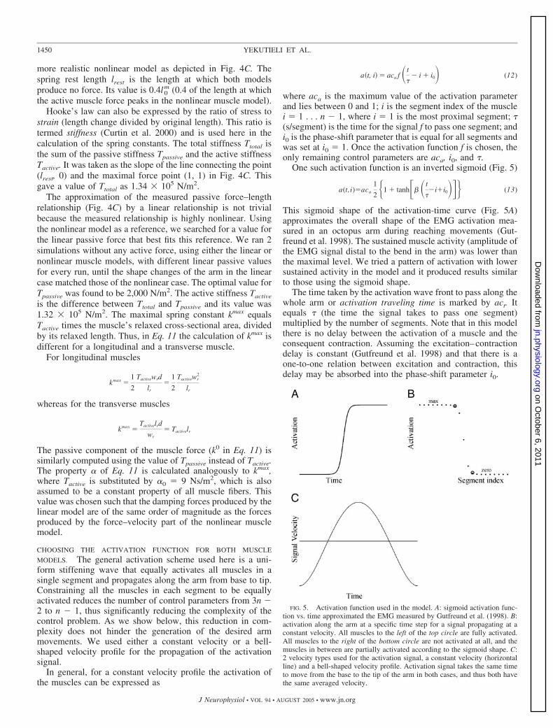
MODELS. The general activation scheme used here is a uni-form stiffening wave that equally activates all muscles in asingle segment and propagates along the arm from base to tip.Constraining all the muscles in each segment to be equallyactivated reduces the number of control parameters from 3n �2 to n � 1, thus significantly reducing the complexity of thecontrol problem. As we show below, this reduction in com-plexity does not hinder the generation of the desired armmovements. We used either a constant velocity or a bell-shaped velocity profile for the propagation of the activationsignal.

In general, for a constant velocity profile the activation ofthe muscles can be expressed as

a�t, i� � aca f �t

� i � i0� (12)

where aca is the maximum value of the activation parameterand lies between 0 and 1; i is the segment index of the musclei 1 . . . n � 1, where i 1 is the most proximal segment; (s/segment) is the time for the signal f to pass one segment; andi0 is the phase-shift parameter that is equal for all segments andwas set at i0 1. Once the activation function f is chosen, theonly remaining control parameters are aca, i0, and .

One such activation function is an inverted sigmoid (Fig. 5)

a(t,i)aca

1

2 �1 � tanh�� � t

�i�i0��� (13)

This sigmoid shape of the activation-time curve (Fig. 5A)approximates the overall shape of the EMG activation mea-sured in an octopus arm during reaching movements (Gut-freund et al. 1998). The sustained muscle activity (amplitude ofthe EMG signal distal to the bend in the arm) was lower thanthe maximal level. We tried a pattern of activation with lowersustained activity in the model and it produced results similarto those using the sigmoid shape.

The time taken by the activation wave front to pass along thewhole arm or activation traveling time is marked by act. Itequals (the time the signal takes to pass one segment)multiplied by the number of segments. Note that in this modelthere is no delay between the activation of a muscle and theconsequent contraction. Assuming the excitation–contractiondelay is constant (Gutfreund et al. 1998) and that there is aone-to-one relation between excitation and contraction, thisdelay may be absorbed into the phase-shift parameter i0.

FIG. 5. Activation function used in the model. A: sigmoid activation func-tion vs. time approximated the EMG measured by Gutfreund et al. (1998). B:activation along the arm at a specific time step for a signal propagating at aconstant velocity. All muscles to the left of the top circle are fully activated.All muscles to the right of the bottom circle are not activated at all, and themuscles in between are partially activated according to the sigmoid shape. C:2 velocity types used for the activation signal, a constant velocity (horizontalline) and a bell-shaped velocity profile. Activation signal takes the same timeto move from the base to the tip of the arm in both cases, and thus both havethe same averaged velocity.

1450 YEKUTIELI ET AL.

J Neurophysiol • VOL 94 • AUGUST 2005 • www.jn.org

on October 6, 2011

jn.physiology.orgD

ownloaded from

We used a minimum jerk polynomial7 for the bell-shapedform of the signal velocity. The maximal signal velocity wasscaled such that the signal traveled along the arm from base totip in a given time with the desired velocity (i.e., the integral ofthe velocity over time equals the length of the arm). Thus fora given total movement time, the average signal velocity wasthe same as the constant velocity (Fig 5C).

R E S U L T S

Drag force

During a reaching movement, the proximal segment of thearm (the part between the bend and the base of the arm) doesnot move and therefore does not suffer from drag forces. Thearea around the bend is relatively small but is exposed to largedrag forces reflecting the large perpendicular coefficient. Incontrast, the distal part (from the bend to the tip of the arm) hason average a much larger surface area, although its drag issmaller because of the nearly 50 times smaller tangentialcoefficient. Measuring the total tangential and perpendiculardrag forces integrated over the entire simulated reaching move-ment revealed that they have almost the same magnitude.

Simulations and experimental results

We now describe behaviors observed in octopuses and theresults of the simulations mimicking such behaviors. In thesimulations, we change the input to the model (analogous to aneural command) by changing the activation amplitude aca andthe activation traveling time act, while keeping all other pa-rameters fixed. Unless otherwise stated, we use the nonlinearmuscle model.

Producing a reaching motion

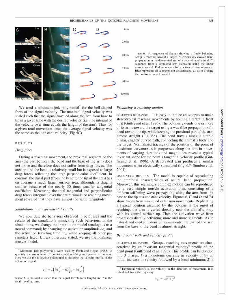
OBSERVED BEHAVIOR. It is easy to induce an octopus to makestereotypical reaching movements by holding a target in frontof it (Gutfreund et al. 1996). The octopus extends one or moreof its arms toward the target using a wavelike propagation of abend toward the tip, while keeping the proximal part of the armalmost straight (Fig. 6A). The bend travels along a simpleplanar, slightly curved path, connecting the animal’s body andthe target. Normalized tracings of the position of the point ofmaximum curvature as it progresses along the arm in move-ments of varying durations and magnitudes reveal a typicalinvariant shape for the point’s tangential velocity profile (Gut-freund et al. 1996). A denervated arm produces a similarmovement when electrically stimulated (Fig. 6B; Sumbre et al.2001).

SIMULATION RESULTS. The model is capable of reproducingthe empirical characteristics of natural bend propagation.Moreover, this seemingly complex motion can be reproducedby a very simple muscle activation plan, consisting of auniform stiffening wave propagating along the arm from thebase to the tip at a constant velocity. Figures 6, C and D and 7Ashow traces from simulated extension movements. Replicatinga typical position assumed by the octopus at the onset ofreaching, the arm is curled dorsally near the animal’s bodywith its ventral surface up. Then the activation wave frontprogresses distally activating more and more segments. As innatural and evoked extension movements, the part of the armfrom the base to the bend is almost straight.

Bend point path and velocity profile

OBSERVED BEHAVIOR. Octopus reaching movements are char-acterized by an invariant tangential velocity8 profile of thebend point (Gutfreund et al. 1996). This profile can be dividedinto 3 phases: 1) a monotonic decrease in velocity or by aninitial increase in velocity followed by a local minimum; 2) a

7 Minimum jerk polynomials were used by Flash and Hogan (1985) toquantify the smoothness of point-to-point reaching movements in humans.Here we use the following polynomial to describe the velocity profile of theactivation signal

v�t� � L�30t2

T 3 � 60t3

T 4 � 30t 4

T 5�where L is the total distance that the signal travels (arm length) and T is thetotal traveling time.

8 Tangential velocity is the velocity in the direction of movement. It iscalculated from the trajectory

Vtan � x2 � y2

FIG. 6. A: sequence of frames showing a freely behavingoctopus reaching toward a target. B: electrically evoked bendpropagation in the denervated arm of a decerebrated animal. C:sequence from a simulated arm extension using the linearmuscle model. Red represents fully activated arm segments.Blue represents all segments not yet activated. D: as in C usingthe nonlinear muscle model.

1451BIOMECHANICS OF THE OCTOPUS REACHING MOVEMENT

J Neurophysiol • VOL 94 • AUGUST 2005 • www.jn.org

on October 6, 2011

jn.physiology.orgD

ownloaded from

monotonic increase in velocity; and 3) a decrease in thevelocity until the bend point disappears (Fig. 8A). Velocityprofiles of denervated arms show similar patterns (Fig. 8B).

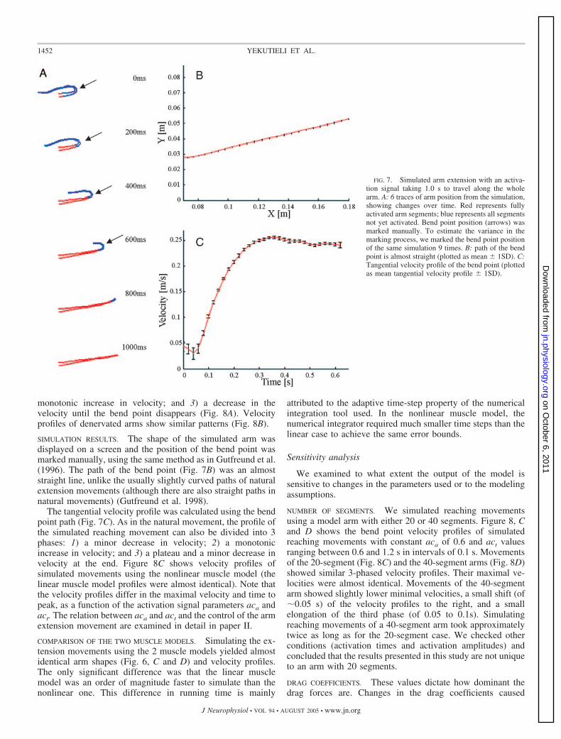
SIMULATION RESULTS. The shape of the simulated arm wasdisplayed on a screen and the position of the bend point wasmarked manually, using the same method as in Gutfreund et al.(1996). The path of the bend point (Fig. 7B) was an almoststraight line, unlike the usually slightly curved paths of naturalextension movements (although there are also straight paths innatural movements) (Gutfreund et al. 1998).

The tangential velocity profile was calculated using the bendpoint path (Fig. 7C). As in the natural movement, the profile ofthe simulated reaching movement can also be divided into 3phases: 1) a minor decrease in velocity; 2) a monotonicincrease in velocity; and 3) a plateau and a minor decrease invelocity at the end. Figure 8C shows velocity profiles ofsimulated movements using the nonlinear muscle model (thelinear muscle model profiles were almost identical). Note thatthe velocity profiles differ in the maximal velocity and time topeak, as a function of the activation signal parameters aca andact. The relation between aca and act and the control of the armextension movement are examined in detail in paper II.

COMPARISON OF THE TWO MUSCLE MODELS. Simulating the ex-tension movements using the 2 muscle models yielded almostidentical arm shapes (Fig. 6, C and D) and velocity profiles.The only significant difference was that the linear musclemodel was an order of magnitude faster to simulate than thenonlinear one. This difference in running time is mainly

attributed to the adaptive time-step property of the numericalintegration tool used. In the nonlinear muscle model, thenumerical integrator required much smaller time steps than thelinear case to achieve the same error bounds.

Sensitivity analysis

We examined to what extent the output of the model issensitive to changes in the parameters used or to the modelingassumptions.

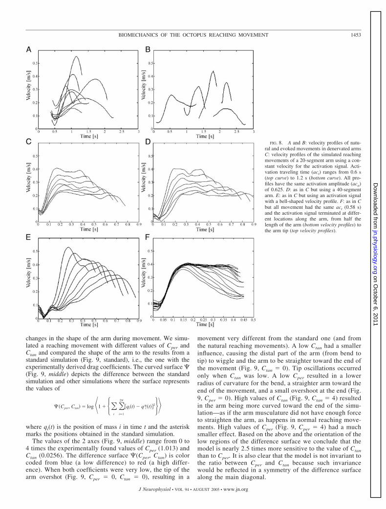
NUMBER OF SEGMENTS. We simulated reaching movementsusing a model arm with either 20 or 40 segments. Figure 8, Cand D shows the bend point velocity profiles of simulatedreaching movements with constant aca of 0.6 and act valuesranging between 0.6 and 1.2 s in intervals of 0.1 s. Movementsof the 20-segment (Fig. 8C) and the 40-segment arms (Fig. 8D)showed similar 3-phased velocity profiles. Their maximal ve-locities were almost identical. Movements of the 40-segmentarm showed slightly lower minimal velocities, a small shift (of�0.05 s) of the velocity profiles to the right, and a smallelongation of the third phase (of 0.05 to 0.1s). Simulatingreaching movements of a 40-segment arm took approximatelytwice as long as for the 20-segment case. We checked otherconditions (activation times and activation amplitudes) andconcluded that the results presented in this study are not uniqueto an arm with 20 segments.

DRAG COEFFICIENTS. These values dictate how dominant thedrag forces are. Changes in the drag coefficients caused

FIG. 7. Simulated arm extension with an activa-tion signal taking 1.0 s to travel along the wholearm. A: 6 traces of arm position from the simulation,showing changes over time. Red represents fullyactivated arm segments; blue represents all segmentsnot yet activated. Bend point position (arrows) wasmarked manually. To estimate the variance in themarking process, we marked the bend point positionof the same simulation 9 times. B: path of the bendpoint is almost straight (plotted as mean 1SD). C:Tangential velocity profile of the bend point (plottedas mean tangential velocity profile 1SD).

1452 YEKUTIELI ET AL.

J Neurophysiol • VOL 94 • AUGUST 2005 • www.jn.org

on October 6, 2011

jn.physiology.orgD

ownloaded from

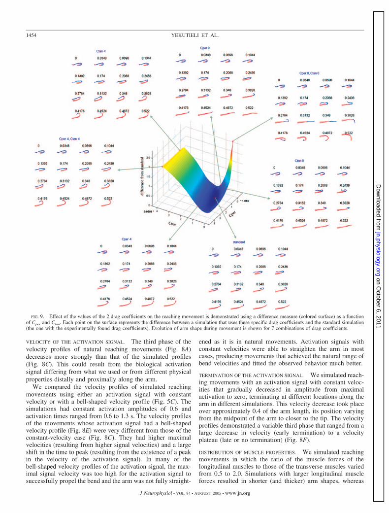
changes in the shape of the arm during movement. We simu-lated a reaching movement with different values of Cper andCtan and compared the shape of the arm to the results from astandard simulation (Fig. 9, standard), i.e., the one with theexperimentally derived drag coefficients. The curved surface �(Fig. 9, middle) depicts the difference between the standardsimulation and other simulations where the surface representsthe values of

��Cper, Ctan� � log �1 � ��t

�i1

2N

�qi�t� � q*i �t��2�

where qi(t) is the position of mass i in time t and the asteriskmarks the positions obtained in the standard simulation.

The values of the 2 axes (Fig. 9, middle) range from 0 to4 times the experimentally found values of Cper (1.013) andCtan (0.0256). The difference surface �(Cper, Ctan) is colorcoded from blue (a low difference) to red (a high differ-ence). When both coefficients were very low, the tip of thearm overshot (Fig. 9, Cper 0, Ctan 0), resulting in a

movement very different from the standard one (and fromthe natural reaching movements). A low Ctan had a smallerinfluence, causing the distal part of the arm (from bend totip) to wiggle and the arm to be straighter toward the end ofthe movement (Fig. 9, Ctan 0). Tip oscillations occurredonly when Ctan was low. A low Cper resulted in a lowerradius of curvature for the bend, a straighter arm toward theend of the movement, and a small overshoot at the end (Fig.9, Cper 0). High values of Ctan (Fig. 9, Ctan 4) resultedin the arm being more curved toward the end of the simu-lation—as if the arm musculature did not have enough forceto straighten the arm, as happens in normal reaching move-ments. High values of Cper (Fig. 9, Cper 4) had a muchsmaller effect. Based on the above and the orientation of thelow regions of the difference surface we conclude that themodel is nearly 2.5 times more sensitive to the value of Ctanthan to Cper. It is also clear that the model is not invariant tothe ratio between Cper and Ctan because such invariancewould be reflected in a symmetry of the difference surfacealong the main diagonal.

FIG. 8. A and B: velocity profiles of natu-ral and evoked movements in denervated armsC: velocity profiles of the simulated reachingmovements of a 20-segment arm using a con-stant velocity for the activation signal. Acti-vation traveling time (act) ranges from 0.6 s(top curve) to 1.2 s (bottom curve). All pro-files have the same activation amplitude (aca)of 0.625. D: as in C but using a 40-segmentarm. E: as in C but using an activation signalwith a bell-shaped velocity profile. F: as in Cbut all movement had the same act (0.58 s)and the activation signal terminated at differ-ent locations along the arm, from half thelength of the arm (bottom velocity profiles) tothe arm tip (top velocity profiles).

1453BIOMECHANICS OF THE OCTOPUS REACHING MOVEMENT

J Neurophysiol • VOL 94 • AUGUST 2005 • www.jn.org

on October 6, 2011

jn.physiology.orgD

ownloaded from

VELOCITY OF THE ACTIVATION SIGNAL. The third phase of thevelocity profiles of natural reaching movements (Fig. 8A)decreases more strongly than that of the simulated profiles(Fig. 8C). This could result from the biological activationsignal differing from what we used or from different physicalproperties distally and proximally along the arm.

We compared the velocity profiles of simulated reachingmovements using either an activation signal with constantvelocity or with a bell-shaped velocity profile (Fig. 5C). Thesimulations had constant activation amplitudes of 0.6 andactivation times ranged from 0.6 to 1.3 s. The velocity profilesof the movements whose activation signal had a bell-shapedvelocity profile (Fig. 8E) were very different from those of theconstant-velocity case (Fig. 8C). They had higher maximalvelocities (resulting from higher signal velocities) and a largeshift in the time to peak (resulting from the existence of a peakin the velocity of the activation signal). In many of thebell-shaped velocity profiles of the activation signal, the max-imal signal velocity was too high for the activation signal tosuccessfully propel the bend and the arm was not fully straight-

ened as it is in natural movements. Activation signals withconstant velocities were able to straighten the arm in mostcases, producing movements that achieved the natural range ofbend velocities and fitted the observed behavior much better.

TERMINATION OF THE ACTIVATION SIGNAL. We simulated reach-ing movements with an activation signal with constant veloc-ities that gradually decreased in amplitude from maximalactivation to zero, terminating at different locations along thearm in different simulations. This velocity decrease took placeover approximately 0.4 of the arm length, its position varyingfrom the midpoint of the arm to closer to the tip. The velocityprofiles demonstrated a variable third phase that ranged from alarge decrease in velocity (early termination) to a velocityplateau (late or no termination) (Fig. 8F).

DISTRIBUTION OF MUSCLE PROPERTIES. We simulated reachingmovements in which the ratio of the muscle forces of thelongitudinal muscles to those of the transverse muscles variedfrom 0.5 to 2.0. Simulations with larger longitudinal muscleforces resulted in shorter (and thicker) arm shapes, whereas

FIG. 9. Effect of the values of the 2 drag coefficients on the reaching movement is demonstrated using a difference measure (colored surface) as a functionof Cper and Ctan. Each point on the surface represents the difference between a simulation that uses these specific drag coefficients and the standard simulation(the one with the experimentally found drag coefficients). Evolution of arm shape during movement is shown for 7 combinations of drag coefficients.

1454 YEKUTIELI ET AL.

J Neurophysiol • VOL 94 • AUGUST 2005 • www.jn.org

on October 6, 2011

jn.physiology.orgD

ownloaded from

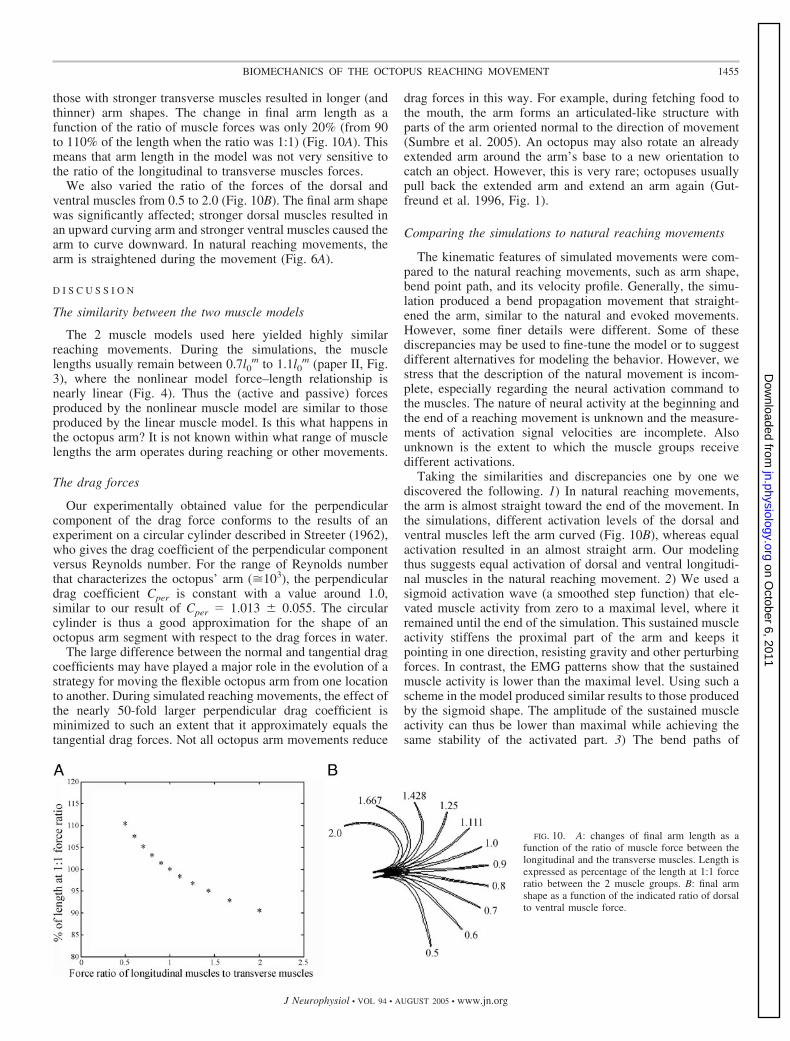
those with stronger transverse muscles resulted in longer (andthinner) arm shapes. The change in final arm length as afunction of the ratio of muscle forces was only 20% (from 90to 110% of the length when the ratio was 1:1) (Fig. 10A). Thismeans that arm length in the model was not very sensitive tothe ratio of the longitudinal to transverse muscles forces.

We also varied the ratio of the forces of the dorsal andventral muscles from 0.5 to 2.0 (Fig. 10B). The final arm shapewas significantly affected; stronger dorsal muscles resulted inan upward curving arm and stronger ventral muscles caused thearm to curve downward. In natural reaching movements, thearm is straightened during the movement (Fig. 6A).

D I S C U S S I O N

The similarity between the two muscle models

The 2 muscle models used here yielded highly similarreaching movements. During the simulations, the musclelengths usually remain between 0.7l0

m to 1.1l0m (paper II, Fig.

3), where the nonlinear model force–length relationship isnearly linear (Fig. 4). Thus the (active and passive) forcesproduced by the nonlinear muscle model are similar to thoseproduced by the linear muscle model. Is this what happens inthe octopus arm? It is not known within what range of musclelengths the arm operates during reaching or other movements.

The drag forces

Our experimentally obtained value for the perpendicularcomponent of the drag force conforms to the results of anexperiment on a circular cylinder described in Streeter (1962),who gives the drag coefficient of the perpendicular componentversus Reynolds number. For the range of Reynolds numberthat characterizes the octopus’ arm (�103), the perpendiculardrag coefficient Cper is constant with a value around 1.0,similar to our result of Cper 1.013 0.055. The circularcylinder is thus a good approximation for the shape of anoctopus arm segment with respect to the drag forces in water.

The large difference between the normal and tangential dragcoefficients may have played a major role in the evolution of astrategy for moving the flexible octopus arm from one locationto another. During simulated reaching movements, the effect ofthe nearly 50-fold larger perpendicular drag coefficient isminimized to such an extent that it approximately equals thetangential drag forces. Not all octopus arm movements reduce

drag forces in this way. For example, during fetching food tothe mouth, the arm forms an articulated-like structure withparts of the arm oriented normal to the direction of movement(Sumbre et al. 2005). An octopus may also rotate an alreadyextended arm around the arm’s base to a new orientation tocatch an object. However, this is very rare; octopuses usuallypull back the extended arm and extend an arm again (Gut-freund et al. 1996, Fig. 1).

Comparing the simulations to natural reaching movements

The kinematic features of simulated movements were com-pared to the natural reaching movements, such as arm shape,bend point path, and its velocity profile. Generally, the simu-lation produced a bend propagation movement that straight-ened the arm, similar to the natural and evoked movements.However, some finer details were different. Some of thesediscrepancies may be used to fine-tune the model or to suggestdifferent alternatives for modeling the behavior. However, westress that the description of the natural movement is incom-plete, especially regarding the neural activation command tothe muscles. The nature of neural activity at the beginning andthe end of a reaching movement is unknown and the measure-ments of activation signal velocities are incomplete. Alsounknown is the extent to which the muscle groups receivedifferent activations.

Taking the similarities and discrepancies one by one wediscovered the following. 1) In natural reaching movements,the arm is almost straight toward the end of the movement. Inthe simulations, different activation levels of the dorsal andventral muscles left the arm curved (Fig. 10B), whereas equalactivation resulted in an almost straight arm. Our modelingthus suggests equal activation of dorsal and ventral longitudi-nal muscles in the natural reaching movement. 2) We used asigmoid activation wave (a smoothed step function) that ele-vated muscle activity from zero to a maximal level, where itremained until the end of the simulation. This sustained muscleactivity stiffens the proximal part of the arm and keeps itpointing in one direction, resisting gravity and other perturbingforces. In contrast, the EMG patterns show that the sustainedmuscle activity is lower than the maximal level. Using such ascheme in the model produced similar results to those producedby the sigmoid shape. The amplitude of the sustained muscleactivity can thus be lower than maximal while achieving thesame stability of the activated part. 3) The bend paths of

FIG. 10. A: changes of final arm length as afunction of the ratio of muscle force between thelongitudinal and the transverse muscles. Length isexpressed as percentage of the length at 1:1 forceratio between the 2 muscle groups. B: final armshape as a function of the indicated ratio of dorsalto ventral muscle force.

1455BIOMECHANICS OF THE OCTOPUS REACHING MOVEMENT

J Neurophysiol • VOL 94 • AUGUST 2005 • www.jn.org

on October 6, 2011

jn.physiology.orgD

ownloaded from

simulated movements are straight and those of natural move-ments are usually slightly curved. This can be attributed to therotation of the arm around its base during natural movementsthat usually occurs at the beginning of the movement and isvariable from movement to movement (unpublished results).We did not model base rotations. 4) The first phase of thevelocity profile of natural movements is variable with someprofiles having a noticeable velocity before the second phase.In contrast, the velocity profiles of the simulated movementsshow a low velocity during the first phase. This difference ismainly explained by the use of tangential velocity profiles todescribe the movement of the bend along the arm. Tangentialvelocity is a scalar value that measures velocity in the directionof the movement. If a bend propagates along the arm creatinga straight spatial path, its tangential velocity and propagationvelocity will be the same. Even if the bend location does notchange at all along the arm, however, movements of the arm inspace will give positive tangential velocities of the bend.Rotating the arm around its base (common in natural move-ments) creates a curved bend path that increases the tangentialvelocity beyond values deriving from bend propagation alone.In contrast, the bend paths of simulated movements are straightand their tangential velocities are directly related to the bendpropagations. 5) The third phase of natural velocity profiles,usually showing a velocity decrease, is much more variablethan in the simulations, where movements with a constantvelocity activation signal show a plateau followed by a smalldecrease. The difference could result from variability in theneural command, such as the timing of signal termination.Termination of the activation signal causes a decrease inmuscle activity and any decrease in the muscle forces propel-ling the bend can cause the observed decrease in bend velocity(Fig. 8F). Anatomically, the muscle cells have similar proper-ties along the arm (unpublished observation). These data do notsupport the decrease in velocity in natural movements asattributed to weaker muscles around at the tip of the arm.

Based on the above, we hypothesize that the velocity ofnatural activation signals probably lies somewhere between theconstant and bell-shaped velocity forms we examined and thatthe amplitude of the activation command decreases toward theend of the movement. The large variability in natural move-ments does not allow us to draw a more precise conclusion.

Finally, this paper describes a dynamic model of the octopusarm that is general enough for modeling other movements inthe octopus, as well as other in muscular hydrostats. Exploringthe hypothesis of a “stiffening wave,” we have shown that anextension movement can be achieved by a very simple controlscheme that minimizes the computational complexity of motorcontrol (which is an important factor for a hyperredundantarm). The stiffening wave was also found to be an efficient wayof moving in water. From here, we can speculate on theevolutionary pressures that led to the development of theoctopus’ neuromuscular system.

In paper II, we use the model developed here to study thebiomechanical details of the extension movements and itscontrol. We show why equal activation of the muscles of anarbitrarily shaped segment transforms it into a symmetricrectangular shape. Such shape changes in several consecutivesegments result in the arm straightening. We then focus on theproperties of the activation signal that creates a wave of musclecontraction. We show that the 2 properties of the activation

signal, its amplitude and its traveling time, are related and themotor control system may use this relation to choose theminimal forces needed to extend an arm according to a desiredkinematic plan. We also show that it is possible to use higherforces to resist external perturbations while keeping the samekinematics. Therefore, our model suggests that the octopus canindependently control 2 major aspects of arm extension move-ments: the kinematics of the movement and its resistance toperturbations. We do not know whether the behaving octopusactually performs according to this prediction.

A P P E N D I X A

Matrices and vectors definitions

The model arm is composed of n mass pairs (total of 2n masses),creating n � 1 segments. M is a diagonal mass matrix where eachmass is represented twice (dimensions: 4n � 4n)

M � �m1

v 0 0 0 . . . 0 00 m1

v 0 0 . . . 0 00 0 m1

d 0 . . . 0 00 0 0 m1

d . . . 0 0� � � � . . . � �

0 0 0 0 . . . mnd 0

0 0 0 0 . . . 0 mnd

�where the superscript v denotes ventral and d denotes dorsal (see Fig.1).

q is the position vector, composed of the coordinates of the 2nmasses (dimensions: 4n � 1)

�x1

v

y1v

x1d

y1d

�

x2nv

y2nv

x2nd

y2nd

�again v denotes ventral and d denotes dorsal.

The same inner organization appears in the force vectors:● fm denotes the muscle forces (4n � 1)

● fg denotes the combined gravity and buoyancy forces (4n � 1)

● fw denotes the water drag forces (4n � 1)

● fc denotes the forces arising from the fixed volume constraints(4n � 1)

● s is the vector of areas of the n � 1 segmentsThe area of each segment was calculated by decomposing the

quadrilateral shape into 2 general triangles and finding their areas

1

2 �� x1

vy1d � x1

dy2d � y1

vx1d � y1

dx2d � x2

dy2v � x2

vy1v � y2

dx2v � y2

vx1v

�

� x2n�1v y2n�1

d � x2n�1d y2n

d � y2n�1v x2n�1

d � y2n�1d x2n

d

� x2nd y2n

v � x2nv y2n�1

v � y2nd x2n

v � y2nv x2n�1

v�

● sc is the vector of values of the constant areas for the n � 1segments

● D is a matrix (n � 1 � 4n) transforming the position vector qto the vector s, which are the areas of the n � 1 segments ofthe arm

1456 YEKUTIELI ET AL.

J Neurophysiol • VOL 94 • AUGUST 2005 • www.jn.org

on October 6, 2011

jn.physiology.orgD

ownloaded from

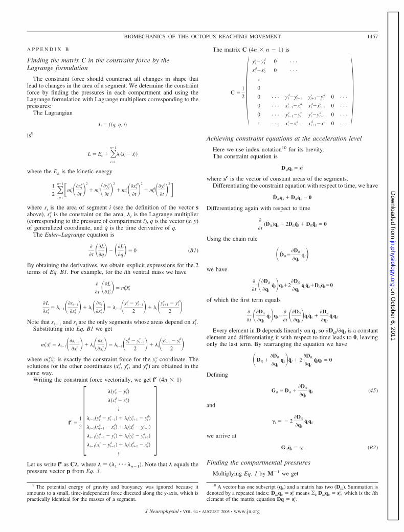
A P P E N D I X B

Finding the matrix C in the constraint force by theLagrange formulation

The constraint force should counteract all changes in shape thatlead to changes in the area of a segment. We determine the constraintforce by finding the pressures in each compartment and using theLagrange formulation with Lagrange multipliers corresponding to thepressures:

The Lagrangian

L � f �q, q, t�

is9

L � Ek � �i1

n�1

�ı�si � sic�

where the Ek is the kinetic energy

1

2 �i1

n�1�miv��xi

v

�t�2

� miv��yi

v

�t�2

� mid��xi

d

�t�2

� mid��yi

d

�t�2�

where si is the area of segment i (see the definition of the vector sabove), si

c is the constraint on the area, �i is the Lagrange multiplier(corresponding to the pressure of compartment i), q is the vector (x, y)of generalized coordinate, and q is the time derivative of q.

The Euler–Lagrange equation is

�

�t��L

�q�� ��L

�q�� 0 (B1)

By obtaining the derivatives, we obtain explicit expressions for the 2terms of Eq. B1. For example, for the ith ventral mass we have

�

�t��L

�xiv�� mi

vxiv

�L

�xiv � �i�1��si�1

�xiv �� �i��si

�xiv�� �i�1�yi

d � yi�1v

2�� �i�yi�1

v � yid

2�

Note that si�1 and si are the only segments whose areas depend on xiv.

Substituting into Eq. B1 we get

mivxi

v � �i�1��si�1

�xiv �� �i��si

�xiv�� �i�1�yi

d � yi�1v

2�� �i�yi�1

v � yid

2�

where mivxi

v is exactly the constraint force for the xiv coordinate. The

solutions for the other coordinates (xid, yi

v, and yid) are obtained in the

same way.Writing the constraint force vectorially, we get fc (4n � 1)

fc �1

2 ���y2

v � y1d�

��x1d � x2

v�

�

�i�1�yid � yi�1

v � � �i�yi�1v � yi

d�

�i�1�xi�1v � xi

d� � �i�xid � yi�1

v �

�i�1�yi�1d � yi

v� � �i�yiv � yi�1

d �

�i�1�xiv � yi�1

d � � �i�xi�1d � xi

v�

�

�Let us write fc as C�, where � (�1 � � � �n�1). Note that � equals thepressure vector p from Eq. 3.

The matrix C (4n � n � 1) is

C �1

2 �y2

v�y1d 0 . . .

x1d�x2

v 0 . . .

�

0

0 . . . yid�yi�1

v yi�1v �yi

d 0 . . .

0 . . . xi�1v �xi

d xid�xi�1

v 0 . . .

0 . . . yi�1v �yi

v yiv�yi�1

d 0 . . .

� . . . xiv�xi�1

d xi�1d �xi

v 0 . . .

�Achieving constraint equations at the acceleration level

Here we use index notation10 for its brevity.The constraint equation is

Dikqk � sic

where sc is the vector of constant areas of the segments.Differentiating the constraint equation with respect to time, we have

Dikqk � Dikqk � 0

Differentiating again with respect to time

�

�t(Dik)qk � 2Dikqk � Dikqk � 0

Using the chain rule

� Dik�Dik

�ql

ql�we have

�

�t��Dik

�ql

ql�qk�2�Dik

�ql

qlqk�Dikqk0

of which the first term equals

�

�t��Dik

�ql

ql�qk�

�t��Dik

�ql�qlqk �

�Dik

�ql

qlqk

Every element in D depends linearly on q, so �Dik/�ql is a constantelement and differentiating it with respect to time leads to 0, leavingonly the last term. By rearranging the equation we have

�Dik ��Dik

�ql

qk�ql � 2�Dik

�ql

qlqk � 0

Defining

Gil � Dik ��Dik

�ql

qk (45)

and

�i � � 2�Dik

�ql

qlqk

we arrive at

Gilqk � �i (B2)

Finding the compartmental pressures

Multiplying Eq. 1 by M�1 we get

9 The potential energy of gravity and buoyancy was ignored because itamounts to a small, time-independent force directed along the y-axis, which ispractically identical for the masses of a segment.

10 A vector has one subscript (qk) and a matrix has two (Dik). Summation isdenoted by a repeated index: Dikqk si

c means ¥k Dikqk sic, which is the ith

element of the matrix equation Dq sic.

1457BIOMECHANICS OF THE OCTOPUS REACHING MOVEMENT

J Neurophysiol • VOL 94 • AUGUST 2005 • www.jn.org

on October 6, 2011

jn.physiology.orgD

ownloaded from

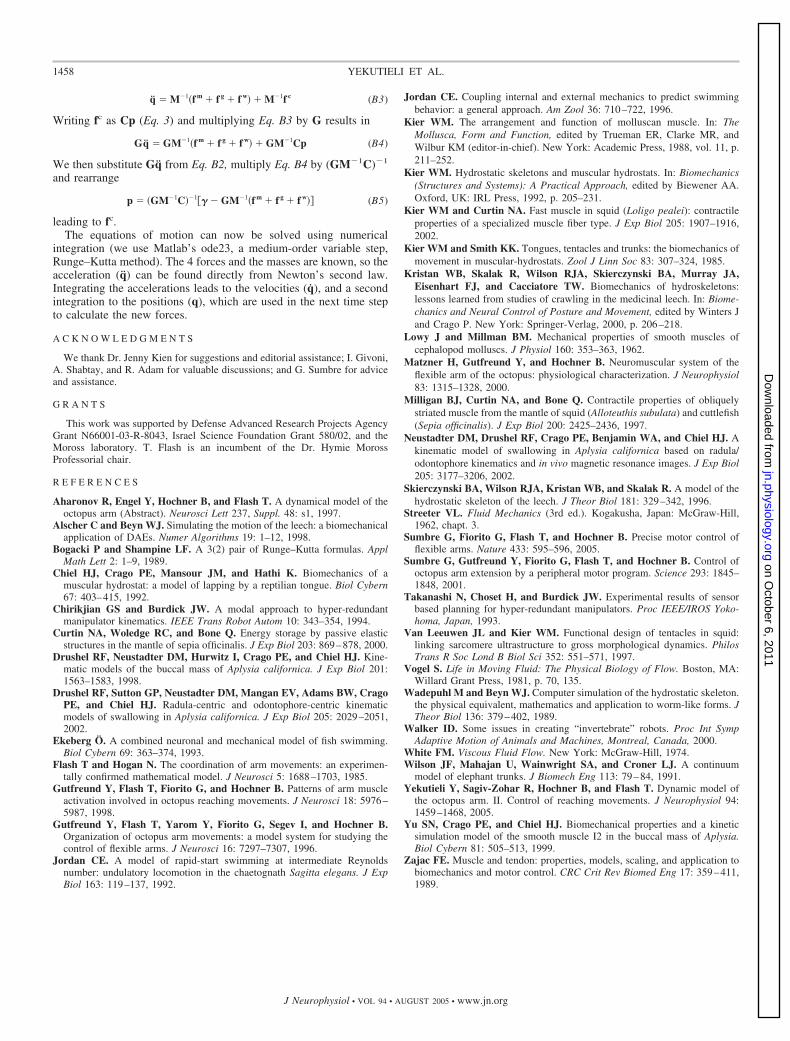
q � M�1�f m � f g � f w� � M�1f c (B3)

Writing fc as Cp (Eq. 3) and multiplying Eq. B3 by G results in

Gq � GM�1�f m � f g � f w� � GM�1Cp (B4)

We then substitute Gq from Eq. B2, multiply Eq. B4 by (GM�1C)�1

and rearrange

p � �GM�1C��1�� � GM�1�f m � f g � f w�� (B5)

leading to fc.The equations of motion can now be solved using numerical

integration (we use Matlab’s ode23, a medium-order variable step,Runge–Kutta method). The 4 forces and the masses are known, so theacceleration (q) can be found directly from Newton’s second law.Integrating the accelerations leads to the velocities (q), and a secondintegration to the positions (q), which are used in the next time stepto calculate the new forces.

A C K N O W L E D G M E N T S

We thank Dr. Jenny Kien for suggestions and editorial assistance; I. Givoni,A. Shabtay, and R. Adam for valuable discussions; and G. Sumbre for adviceand assistance.

G R A N T S

This work was supported by Defense Advanced Research Projects AgencyGrant N66001-03-R-8043, Israel Science Foundation Grant 580/02, and theMoross laboratory. T. Flash is an incumbent of the Dr. Hymie MorossProfessorial chair.

R E F E R E N C E S

Aharonov R, Engel Y, Hochner B, and Flash T. A dynamical model of theoctopus arm (Abstract). Neurosci Lett 237, Suppl. 48: s1, 1997.

Alscher C and Beyn WJ. Simulating the motion of the leech: a biomechanicalapplication of DAEs. Numer Algorithms 19: 1–12, 1998.

Bogacki P and Shampine LF. A 3(2) pair of Runge–Kutta formulas. ApplMath Lett 2: 1–9, 1989.

Chiel HJ, Crago PE, Mansour JM, and Hathi K. Biomechanics of amuscular hydrostat: a model of lapping by a reptilian tongue. Biol Cybern67: 403–415, 1992.

Chirikjian GS and Burdick JW. A modal approach to hyper-redundantmanipulator kinematics. IEEE Trans Robot Autom 10: 343–354, 1994.

Curtin NA, Woledge RC, and Bone Q. Energy storage by passive elasticstructures in the mantle of sepia officinalis. J Exp Biol 203: 869–878, 2000.

Drushel RF, Neustadter DM, Hurwitz I, Crago PE, and Chiel HJ. Kine-matic models of the buccal mass of Aplysia californica. J Exp Biol 201:1563–1583, 1998.

Drushel RF, Sutton GP, Neustadter DM, Mangan EV, Adams BW, CragoPE, and Chiel HJ. Radula-centric and odontophore-centric kinematicmodels of swallowing in Aplysia californica. J Exp Biol 205: 2029–2051,2002.

Ekeberg O. A combined neuronal and mechanical model of fish swimming.Biol Cybern 69: 363–374, 1993.

Flash T and Hogan N. The coordination of arm movements: an experimen-tally confirmed mathematical model. J Neurosci 5: 1688–1703, 1985.

Gutfreund Y, Flash T, Fiorito G, and Hochner B. Patterns of arm muscleactivation involved in octopus reaching movements. J Neurosci 18: 5976–5987, 1998.

Gutfreund Y, Flash T, Yarom Y, Fiorito G, Segev I, and Hochner B.Organization of octopus arm movements: a model system for studying thecontrol of flexible arms. J Neurosci 16: 7297–7307, 1996.

Jordan CE. A model of rapid-start swimming at intermediate Reynoldsnumber: undulatory locomotion in the chaetognath Sagitta elegans. J ExpBiol 163: 119–137, 1992.

Jordan CE. Coupling internal and external mechanics to predict swimmingbehavior: a general approach. Am Zool 36: 710–722, 1996.

Kier WM. The arrangement and function of molluscan muscle. In: TheMollusca, Form and Function, edited by Trueman ER, Clarke MR, andWilbur KM (editor-in-chief). New York: Academic Press, 1988, vol. 11, p.211–252.

Kier WM. Hydrostatic skeletons and muscular hydrostats. In: Biomechanics(Structures and Systems): A Practical Approach, edited by Biewener AA.Oxford, UK: IRL Press, 1992, p. 205–231.

Kier WM and Curtin NA. Fast muscle in squid (Loligo pealei): contractileproperties of a specialized muscle fiber type. J Exp Biol 205: 1907–1916,2002.

Kier WM and Smith KK. Tongues, tentacles and trunks: the biomechanics ofmovement in muscular-hydrostats. Zool J Linn Soc 83: 307–324, 1985.

Kristan WB, Skalak R, Wilson RJA, Skierczynski BA, Murray JA,Eisenhart FJ, and Cacciatore TW. Biomechanics of hydroskeletons:lessons learned from studies of crawling in the medicinal leech. In: Biome-chanics and Neural Control of Posture and Movement, edited by Winters Jand Crago P. New York: Springer-Verlag, 2000, p. 206–218.

Lowy J and Millman BM. Mechanical properties of smooth muscles ofcephalopod molluscs. J Physiol 160: 353–363, 1962.

Matzner H, Gutfreund Y, and Hochner B. Neuromuscular system of theflexible arm of the octopus: physiological characterization. J Neurophysiol83: 1315–1328, 2000.

Milligan BJ, Curtin NA, and Bone Q. Contractile properties of obliquelystriated muscle from the mantle of squid (Alloteuthis subulata) and cuttlefish(Sepia officinalis). J Exp Biol 200: 2425–2436, 1997.

Neustadter DM, Drushel RF, Crago PE, Benjamin WA, and Chiel HJ. Akinematic model of swallowing in Aplysia californica based on radula/odontophore kinematics and in vivo magnetic resonance images. J Exp Biol205: 3177–3206, 2002.

Skierczynski BA, Wilson RJA, Kristan WB, and Skalak R. A model of thehydrostatic skeleton of the leech. J Theor Biol 181: 329–342, 1996.

Streeter VL. Fluid Mechanics (3rd ed.). Kogakusha, Japan: McGraw-Hill,1962, chapt. 3.

Sumbre G, Fiorito G, Flash T, and Hochner B. Precise motor control offlexible arms. Nature 433: 595–596, 2005.

Sumbre G, Gutfreund Y, Fiorito G, Flash T, and Hochner B. Control ofoctopus arm extension by a peripheral motor program. Science 293: 1845–1848, 2001.

Takanashi N, Choset H, and Burdick JW. Experimental results of sensorbased planning for hyper-redundant manipulators. Proc IEEE/IROS Yoko-homa, Japan, 1993.

Van Leeuwen JL and Kier WM. Functional design of tentacles in squid:linking sarcomere ultrastructure to gross morphological dynamics. PhilosTrans R Soc Lond B Biol Sci 352: 551–571, 1997.

Vogel S. Life in Moving Fluid: The Physical Biology of Flow. Boston, MA:Willard Grant Press, 1981, p. 70, 135.

Wadepuhl M and Beyn WJ. Computer simulation of the hydrostatic skeleton.the physical equivalent, mathematics and application to worm-like forms. JTheor Biol 136: 379–402, 1989.

Walker ID. Some issues in creating “invertebrate” robots. Proc Int SympAdaptive Motion of Animals and Machines, Montreal, Canada, 2000.

White FM. Viscous Fluid Flow. New York: McGraw-Hill, 1974.Wilson JF, Mahajan U, Wainwright SA, and Croner LJ. A continuum

model of elephant trunks. J Biomech Eng 113: 79–84, 1991.Yekutieli Y, Sagiv-Zohar R, Hochner B, and Flash T. Dynamic model of

the octopus arm. II. Control of reaching movements. J Neurophysiol 94:1459–1468, 2005.

Yu SN, Crago PE, and Chiel HJ. Biomechanical properties and a kineticsimulation model of the smooth muscle I2 in the buccal mass of Aplysia.Biol Cybern 81: 505–513, 1999.

Zajac FE. Muscle and tendon: properties, models, scaling, and application tobiomechanics and motor control. CRC Crit Rev Biomed Eng 17: 359–411,1989.

1458 YEKUTIELI ET AL.

J Neurophysiol • VOL 94 • AUGUST 2005 • www.jn.org

on October 6, 2011

jn.physiology.orgD

ownloaded from