Dynamic Mesh Refining and Iterative Substructure Method … · Dynamic Mesh Refining and Iterative Substructure Method 191 programming. Figure 3 shows the refining process of a

Copyright © 2015 Tech Science Press CMES, vol.106, no.3, pp.187-201, 2015

Dynamic Mesh Refining and Iterative SubstructureMethod for Fillet Welding Thermo-Mechanical Analysis

Hui Huang and Hidekazu Murakawa

Abstract: Dynamic mesh refining method (DMRM) developed previously wasextended to multi-level refinement, and employed to perform thermal-mechanicalanalysis of fillet welding. The DMRM has been successfully incorporated withanother efficient technique, the iterative substructure method (ISM) to greatly en-hance the computation speed of welding simulation. The basic concept, hierarchi-cal modeling and computation flowchart are described for the proposed method.A flange-to-pipe welding problem has been solved with a commercial code andthe novel method to demonstrate its high accuracy and efficiency. Furthermore,the numerical analysis was performed on a large scale stiffened welding structure,and comparison of welding deformation between simulation and measurement wasshown.

Keywords: Mesh Refining, Fillet welding, Welding deformation, Substructure,Simulation.

1 Introduction

Owing to the development of computer technology, numerical simulation of weld-ing deformation and residual stress is now receiving increasing attention from aca-demic and engineering fields. The thermo-mechanical finite element analysis canwell reproduce the stress and strain field under complex conditions, such as beadshape, welding sequence and component interaction. However, the strong nonlin-earity and transient feature associated with the welding process prohibit the appli-cation of presently available tools to large industrial scale problems. In the past twodecades, extensive efforts to improve the computation performance have been paidon different techniques such as modeling scheme and solution algorithm.

Sarkani (2000), Deng (2006) and Barsoum (2009) studied the formation of thewelding residual stresses by 2D and 3D simulations separately, and they foundthat 2D prediction shows good agreement with measurements, hence computa-tional time can be greatly reduced compared with 3D simulations. Näsström (1992)

188 Copyright © 2015 Tech Science Press CMES, vol.106, no.3, pp.187-201, 2015

modeled a welding component using solid elements in and near the weld but shellelements elsewhere. The combination of solid elements and shell elements couldreduce the number of degree of freedom (DOF) in the welding problem.

Karlsson (2011) and Bhatti (2012) employed the block-dumping approach in thermo-mechanical analysis for prediction of welding deformation and residual stresses.The approach can reduce the number of time steps significantly and keep satisfac-tory accuracy in welding simulation. Ding (2014) employed the concept of peaktemperature to determine the residual stress and deformation during wire and arcadditive manufacturing.

Biswas and Mandal (2008) developed an analysis methodology based on the quasi-stationary nature of welding and symmetry of model for studying the distortionpattern of orthogonally stiffened large plate panels. Moreover, a comparison wasmade for prediction of welding distortions in a stiffened plate panel among threedifferent FE approaches, namely the transient thermomechanical analysis and twodifferent equivalent techniques, inherent strain method and transient cooling phaseanalysis by Biswas and Mandal (2009).

In aspect of solution algorithm, Murakawa (2005) proposed the iterative substruc-ture method which maintains high accuracy for various cases. The basic idea is tosolve the weakly nonlinear region A and strongly nonlinear region B interactively,and complete the iteration until the residual force on the interface between regionA and region B vanishes. Nishikawa (2007) presented several actual applicationsof ISM, the high accuracy and efficiency had been well validated. It has also beenpointed out that the ISM is most efficient for models with DOF less than 1 mil-lion, because the computation time of region A is primary for large scale problem(Murakawa, 2015). Bhatti (2014) employed the substructure approach in analysisof a large complex welded structure, and they obtained welding residual stresseswith acceptable accuracy in much shorter time than direct solution with full struc-ture. Ikushima and Shibahara (2014) applied the explicit scheme in solving weldingthermal mechanical problem with a GPU acceleration technique.

In the framework of adaptive methods, Brown and Song (1993) presented theremeshing method and substructure method using a shell model. Heating alongthe edge of a plate was analyzed, and a reduction of computation time of anal-ysis without remeshing to one seventh was realized with qualitative accuracy inresults. Lendgren (1997) developed the 3D remeshing technique by means of anode-number variable element to fit the mesh transition zone. An improvement ofcomputation efficiency by about 4 times was achieved. Duranton (2004) proposedan adaptive meshing technique with constraint elements to decrease the computa-tion costs while keeping good accuracy of the results. Regarding these remesh-ing methods, mesh coarsening effect on residual stress and plastic strain was not

Dynamic Mesh Refining and Iterative Substructure Method 189

discussed, although interpolation and mapping procedures generally induce non-negligible error in solution variables in strongly nonlinear problems.

Huang and Murakawa (2013) developed the dynamic mesh refining method (DMRM)based on the characteristic of welding problems. A background mesh was origi-nally proposed to save and update the values of stress and strain. Enhancement oncomputation efficiency by 6 times had been realized with good accuracy by usingonelevel refinement.

Recently, the DMRM was extended to refinement in multi-level hierarchical mode,so the number of DOFs could be further decreased. Moreover, the DMRM wasincorporated with the ISM to establish a powerful tool for thermo-mechanical anal-ysis. Two examples of fillet welding were shown in the present study, and a com-parison between the in-house code JWRIAN* using multi-level DMRM-ISM, anda general purpose code ABAQUS had been made to validate the accuracy and effi-ciency of proposed method.

2 Dynamic mesh refining method with multi-level refinement

2.1 Basic concept

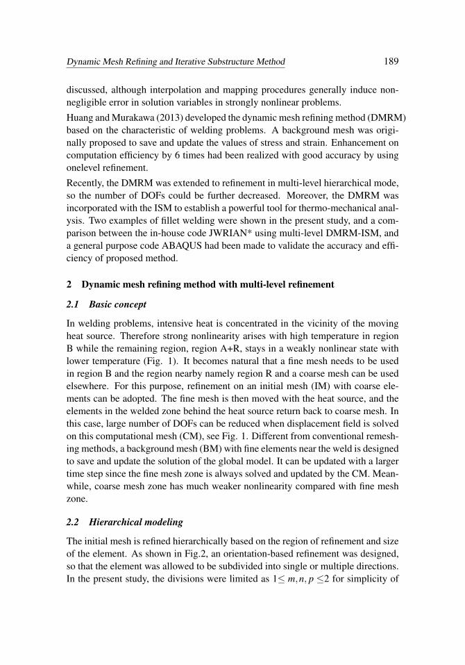
In welding problems, intensive heat is concentrated in the vicinity of the movingheat source. Therefore strong nonlinearity arises with high temperature in regionB while the remaining region, region A+R, stays in a weakly nonlinear state withlower temperature (Fig. 1). It becomes natural that a fine mesh needs to be usedin region B and the region nearby namely region R and a coarse mesh can be usedelsewhere. For this purpose, refinement on an initial mesh (IM) with coarse ele-ments can be adopted. The fine mesh is then moved with the heat source, and theelements in the welded zone behind the heat source return back to coarse mesh. Inthis case, large number of DOFs can be reduced when displacement field is solvedon this computational mesh (CM), see Fig. 1. Different from conventional remesh-ing methods, a background mesh (BM) with fine elements near the weld is designedto save and update the solution of the global model. It can be updated with a largertime step since the fine mesh zone is always solved and updated by the CM. Mean-while, coarse mesh zone has much weaker nonlinearity compared with fine meshzone.

2.2 Hierarchical modeling

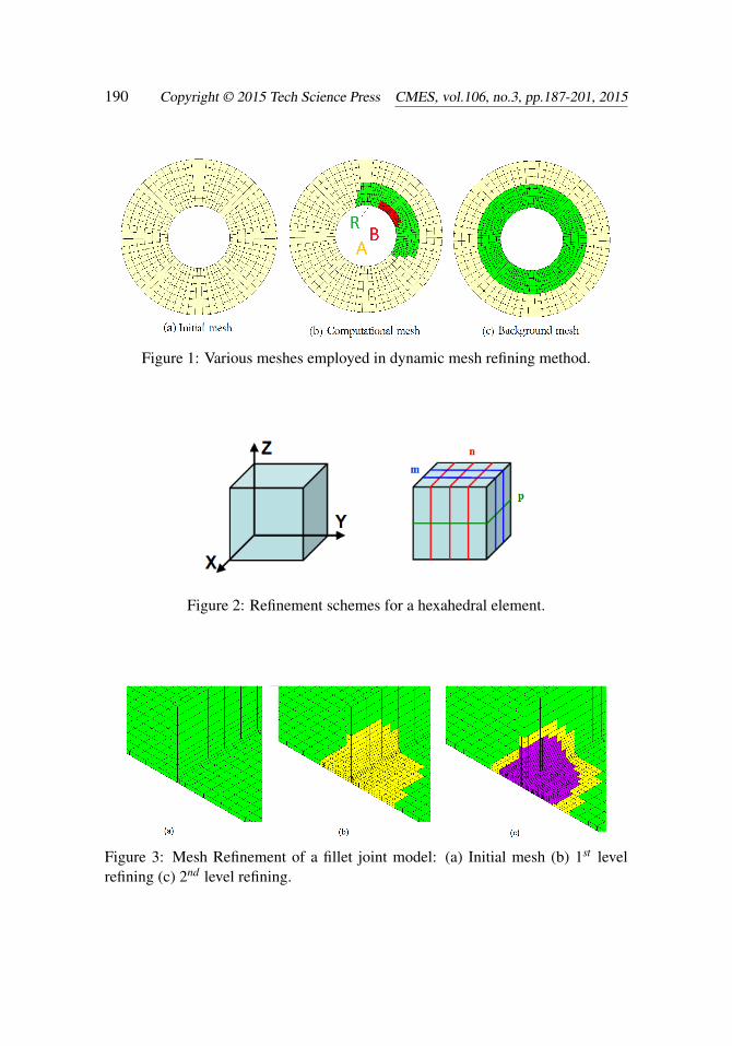
The initial mesh is refined hierarchically based on the region of refinement and sizeof the element. As shown in Fig.2, an orientation-based refinement was designed,so that the element was allowed to be subdivided into single or multiple directions.In the present study, the divisions were limited as 1≤ m,n, p ≤2 for simplicity of


Figure 1: Various meshes employed in dynamic mesh refining method.

Figure 2: Refinement schemes for a hexahedral element.

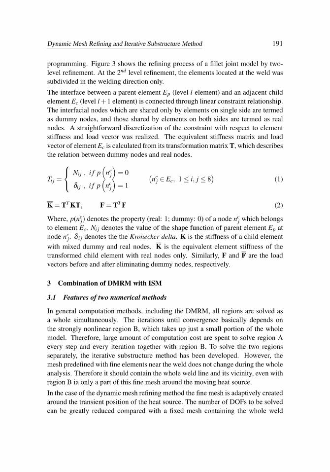
Figure 3: Mesh Refinement of a fillet joint model: (a) Initial mesh (b) 1st levelrefining (c) 2nd level refining.


programming. Figure 3 shows the refining process of a fillet joint model by two-level refinement. At the 2nd level refinement, the elements located at the weld wassubdivided in the welding direction only.

The interface between a parent element Ep (level l element) and an adjacent childelement Ec (level l+1 element) is connected through linear constraint relationship.The interfacial nodes which are shared only by elements on single side are termedas dummy nodes, and those shared by elements on both sides are termed as realnodes. A straightforward discretization of the constraint with respect to elementstiffness and load vector was realized. The equivalent stiffness matrix and loadvector of element Ec is calculated from its transformation matrix T, which describesthe relation between dummy nodes and real nodes.

Ti j =

Ni j , i f p(

ncj

)= 0

δi j , i f p(

ncj

)= 1

(nc

j ∈ Ec, 1≤ i, j ≤ 8)

(1)

K = TT KT, F = TT F (2)

Where, p(ncj) denotes the property (real: 1; dummy: 0) of a node nc

j which belongsto element Ec. Ni j denotes the value of the shape function of parent element Ep atnode nc

j. δ i j denotes the the Kronecker delta. K is the stiffness of a child elementwith mixed dummy and real nodes. K is the equivalent element stiffness of thetransformed child element with real nodes only. Similarly, F and F are the loadvectors before and after eliminating dummy nodes, respectively.

3 Combination of DMRM with ISM

3.1 Features of two numerical methods

In general computation methods, including the DMRM, all regions are solved asa whole simultaneously. The iterations until convergence basically depends onthe strongly nonlinear region B, which takes up just a small portion of the wholemodel. Therefore, large amount of computation cost are spent to solve region Aevery step and every iteration together with region B. To solve the two regionsseparately, the iterative substructure method has been developed. However, themesh predefined with fine elements near the weld does not change during the wholeanalysis. Therefore it should contain the whole weld line and its vicinity, even withregion B ia only a part of this fine mesh around the moving heat source.

In the case of the dynamic mesh refining method the fine mesh is adaptively createdaround the transient position of the heat source. The number of DOFs to be solvedcan be greatly reduced compared with a fixed mesh containing the whole weld


line. Therefore, it can be seen that, the dynamic mesh refining method reduces theunknowns in the global region A by having coarse elements at and around the weldline away from the heat source; and the iterative substructure method deals withnonlinearity in the local region B without having to solve region A in each stepand each iteration with region B. Combine the two different techniques has largepotential in solving large scale thermo-mechanical problems.

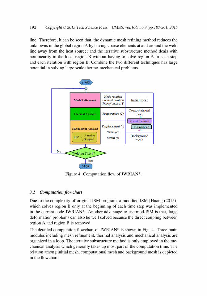
Figure 4: Computation flow of JWRIAN*.

3.2 Computation flowchart

Due to the complexity of original ISM program, a modified ISM [Huang (2015)]which solves region B only at the beginning of each time step was implementedin the current code JWRIAN*. Another advantage to use mod-ISM is that, largedeformation problems can also be well solved because the direct coupling betweenregion A and region B is removed.

The detailed computation flowchart of JWRIAN* is shown in Fig. 4. Three mainmodules including mesh refinement, thermal analysis and mechanical analysis areorganized in a loop. The iterative substructure method is only employed in the me-chanical analysis which generally takes up most part of the computation time. Therelation among initial mesh, computational mesh and background mesh is depictedin the flowchart.


4 Examples and Discussions

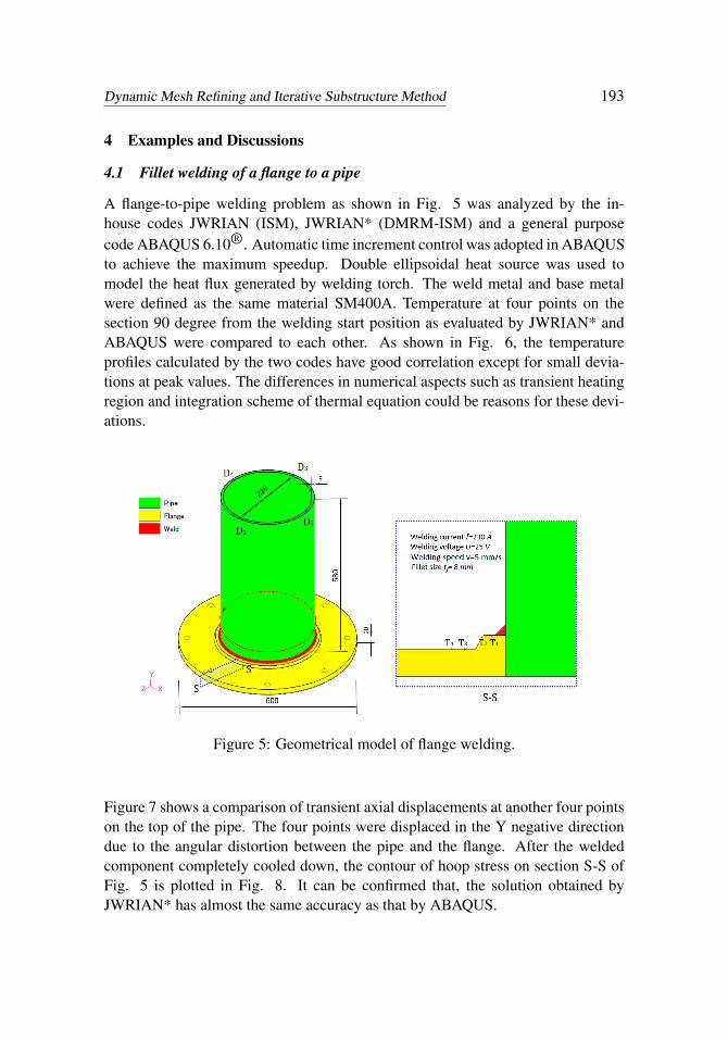
4.1 Fillet welding of a flange to a pipe

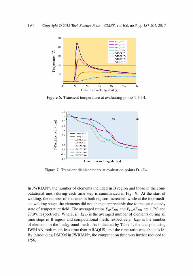
A flange-to-pipe welding problem as shown in Fig. 5 was analyzed by the in-house codes JWRIAN (ISM), JWRIAN* (DMRM-ISM) and a general purposecode ABAQUS 6.10®. Automatic time increment control was adopted in ABAQUSto achieve the maximum speedup. Double ellipsoidal heat source was used tomodel the heat flux generated by welding torch. The weld metal and base metalwere defined as the same material SM400A. Temperature at four points on thesection 90 degree from the welding start position as evaluated by JWRIAN* andABAQUS were compared to each other. As shown in Fig. 6, the temperatureprofiles calculated by the two codes have good correlation except for small devia-tions at peak values. The differences in numerical aspects such as transient heatingregion and integration scheme of thermal equation could be reasons for these devi-ations.

Figure 5: Geometrical model of flange welding.

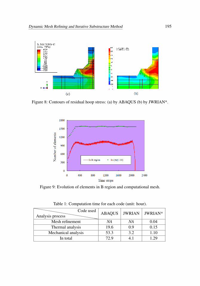
Figure 7 shows a comparison of transient axial displacements at another four pointson the top of the pipe. The four points were displaced in the Y negative directiondue to the angular distortion between the pipe and the flange. After the weldedcomponent completely cooled down, the contour of hoop stress on section S-S ofFig. 5 is plotted in Fig. 8. It can be confirmed that, the solution obtained byJWRIAN* has almost the same accuracy as that by ABAQUS.


Figure 6: Transient temperature at evaluating points T1-T4.

Figure 7: Transient displacements at evaluation points D1-D4.

In JWRIAN*, the number of elements included in B region and those in the com-putational mesh during each time step is summarized in Fig. 9. At the start ofwelding, the number of elements in both regions increased; while at the intermedi-ate welding stage, the elements did not change appreciably due to the quasi-steadystate of temperature field. The averaged ratios EB/EBM and ECM/EBM are 1.7% and27.9% respectively. Where, EB,ECM is the averaged number of elements during alltime steps in B region and computational mesh, respectively. EBM is the numberof elements in the background mesh. As indicated by Table 1, the analysis usingJWRIAN took much less time than ABAQUS, and the time ratio was about 1/18.By introducing DMRM in JWRIAN*, the computation time was further reduced to1/56.


Figure 8: Contours of residual hoop stress: (a) by ABAQUS (b) by JWRIAN*.

Figure 9: Evolution of elements in B region and computational mesh.

Table 1: Computation time for each code (unit: hour).hhhhhhhhhhhhhhhhhAnalysis process

Code usedABAQUS JWRIAN JWRIAN*

Mesh refinement NA NA 0.04Thermal analysis 19.6 0.9 0.15

Mechanical analysis 53.3 3.2 1.10In total 72.9 4.1 1.29


4.2 Welding of a stiffened panel

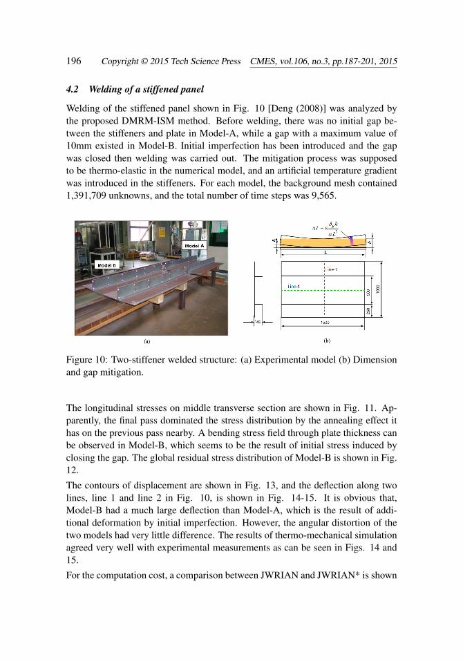
Welding of the stiffened panel shown in Fig. 10 [Deng (2008)] was analyzed bythe proposed DMRM-ISM method. Before welding, there was no initial gap be-tween the stiffeners and plate in Model-A, while a gap with a maximum value of10mm existed in Model-B. Initial imperfection has been introduced and the gapwas closed then welding was carried out. The mitigation process was supposedto be thermo-elastic in the numerical model, and an artificial temperature gradientwas introduced in the stiffeners. For each model, the background mesh contained1,391,709 unknowns, and the total number of time steps was 9,565.

Figure 10: Two-stiffener welded structure: (a) Experimental model (b) Dimensionand gap mitigation.

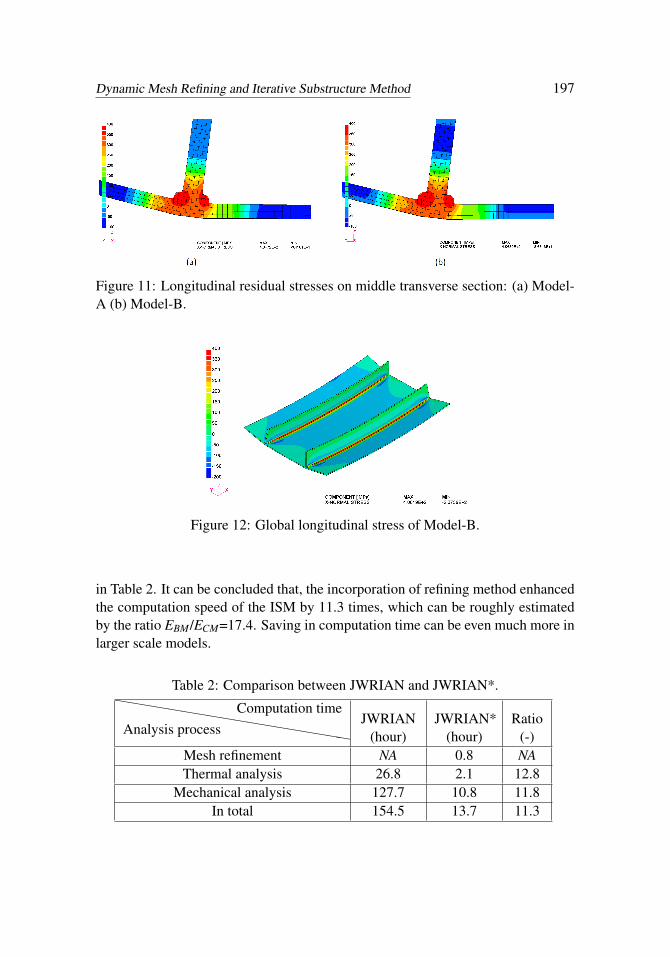
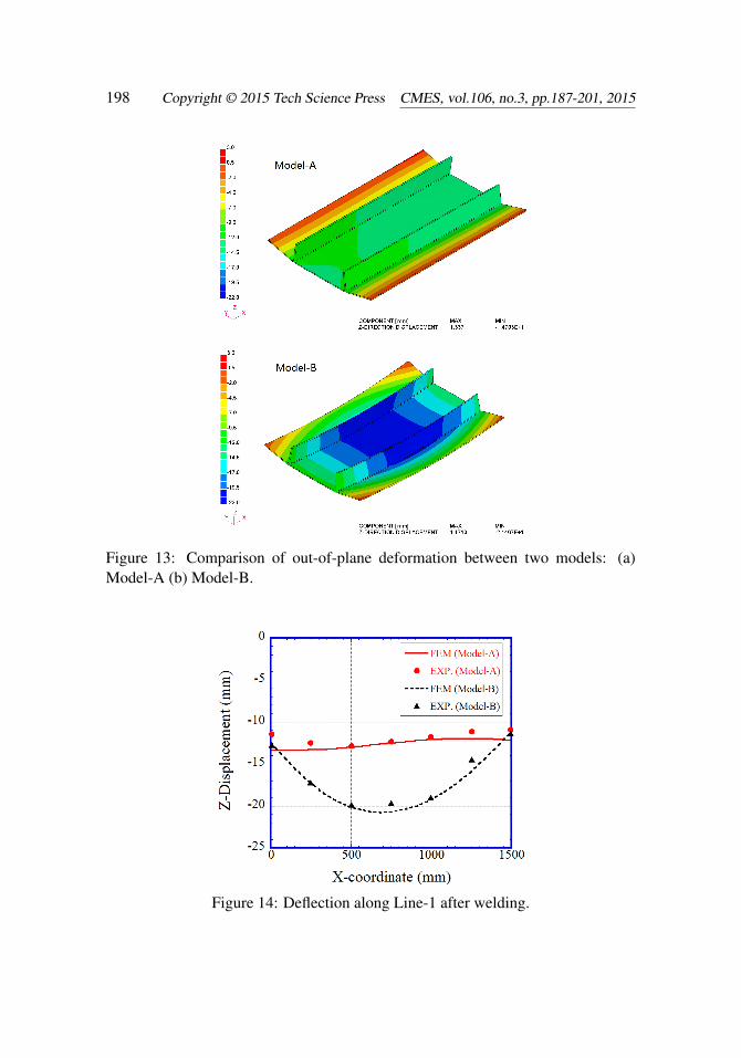
The longitudinal stresses on middle transverse section are shown in Fig. 11. Ap-parently, the final pass dominated the stress distribution by the annealing effect ithas on the previous pass nearby. A bending stress field through plate thickness canbe observed in Model-B, which seems to be the result of initial stress induced byclosing the gap. The global residual stress distribution of Model-B is shown in Fig.12.

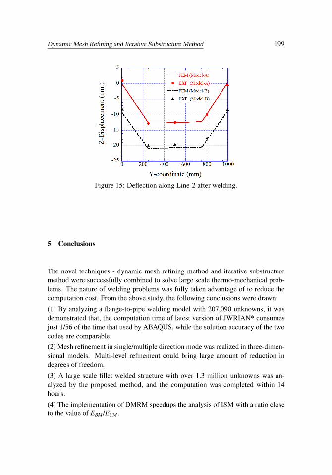
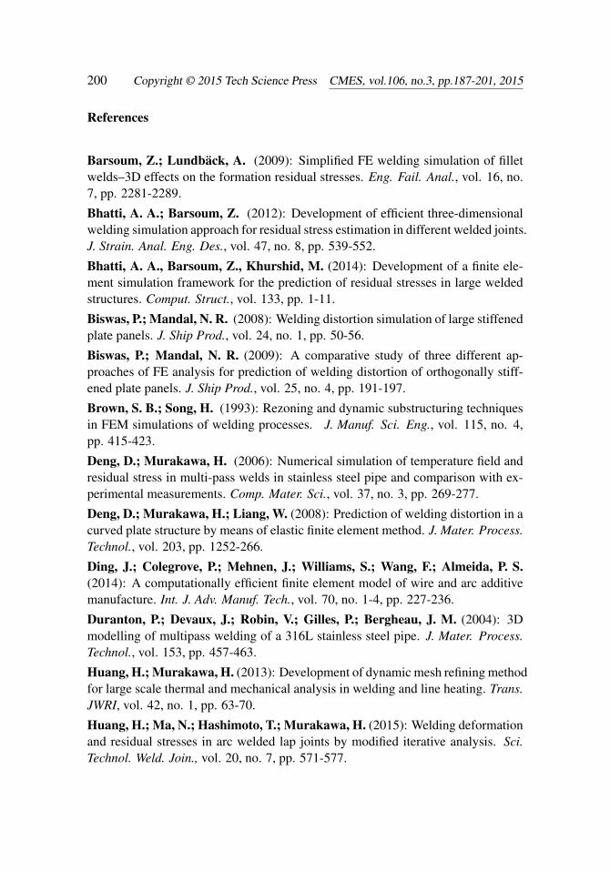
The contours of displacement are shown in Fig. 13, and the deflection along twolines, line 1 and line 2 in Fig. 10, is shown in Fig. 14-15. It is obvious that,Model-B had a much large deflection than Model-A, which is the result of addi-tional deformation by initial imperfection. However, the angular distortion of thetwo models had very little difference. The results of thermo-mechanical simulationagreed very well with experimental measurements as can be seen in Figs. 14 and15.

For the computation cost, a comparison between JWRIAN and JWRIAN* is shown


Figure 11: Longitudinal residual stresses on middle transverse section: (a) Model-A (b) Model-B.

Figure 12: Global longitudinal stress of Model-B.

in Table 2. It can be concluded that, the incorporation of refining method enhancedthe computation speed of the ISM by 11.3 times, which can be roughly estimatedby the ratio EBM/ECM=17.4. Saving in computation time can be even much more inlarger scale models.

Table 2: Comparison between JWRIAN and JWRIAN*.hhhhhhhhhhhhhhhhhhAnalysis process

Computation timeJWRIAN

(hour)JWRIAN*

(hour)Ratio

(-)Mesh refinement NA 0.8 NAThermal analysis 26.8 2.1 12.8

Mechanical analysis 127.7 10.8 11.8In total 154.5 13.7 11.3


Figure 13: Comparison of out-of-plane deformation between two models: (a)Model-A (b) Model-B.

Figure 14: Deflection along Line-1 after welding.


Figure 15: Deflection along Line-2 after welding.

5 Conclusions

The novel techniques - dynamic mesh refining method and iterative substructuremethod were successfully combined to solve large scale thermo-mechanical prob-lems. The nature of welding problems was fully taken advantage of to reduce thecomputation cost. From the above study, the following conclusions were drawn:

(1) By analyzing a flange-to-pipe welding model with 207,090 unknowns, it wasdemonstrated that, the computation time of latest version of JWRIAN* consumesjust 1/56 of the time that used by ABAQUS, while the solution accuracy of the twocodes are comparable.

(2) Mesh refinement in single/multiple direction mode was realized in three-dimen-sional models. Multi-level refinement could bring large amount of reduction indegrees of freedom.

(3) A large scale fillet welded structure with over 1.3 million unknowns was an-alyzed by the proposed method, and the computation was completed within 14hours.

(4) The implementation of DMRM speedups the analysis of ISM with a ratio closeto the value of EBM/ECM.


References

Barsoum, Z.; Lundbäck, A. (2009): Simplified FE welding simulation of filletwelds–3D effects on the formation residual stresses. Eng. Fail. Anal., vol. 16, no.7, pp. 2281-2289.

Bhatti, A. A.; Barsoum, Z. (2012): Development of efficient three-dimensionalwelding simulation approach for residual stress estimation in different welded joints.J. Strain. Anal. Eng. Des., vol. 47, no. 8, pp. 539-552.

Bhatti, A. A., Barsoum, Z., Khurshid, M. (2014): Development of a finite ele-ment simulation framework for the prediction of residual stresses in large weldedstructures. Comput. Struct., vol. 133, pp. 1-11.

Biswas, P.; Mandal, N. R. (2008): Welding distortion simulation of large stiffenedplate panels. J. Ship Prod., vol. 24, no. 1, pp. 50-56.

Biswas, P.; Mandal, N. R. (2009): A comparative study of three different ap-proaches of FE analysis for prediction of welding distortion of orthogonally stiff-ened plate panels. J. Ship Prod., vol. 25, no. 4, pp. 191-197.

Brown, S. B.; Song, H. (1993): Rezoning and dynamic substructuring techniquesin FEM simulations of welding processes. J. Manuf. Sci. Eng., vol. 115, no. 4,pp. 415-423.

Deng, D.; Murakawa, H. (2006): Numerical simulation of temperature field andresidual stress in multi-pass welds in stainless steel pipe and comparison with ex-perimental measurements. Comp. Mater. Sci., vol. 37, no. 3, pp. 269-277.

Deng, D.; Murakawa, H.; Liang, W. (2008): Prediction of welding distortion in acurved plate structure by means of elastic finite element method. J. Mater. Process.Technol., vol. 203, pp. 1252-266.

Ding, J.; Colegrove, P.; Mehnen, J.; Williams, S.; Wang, F.; Almeida, P. S.(2014): A computationally efficient finite element model of wire and arc additivemanufacture. Int. J. Adv. Manuf. Tech., vol. 70, no. 1-4, pp. 227-236.

Duranton, P.; Devaux, J.; Robin, V.; Gilles, P.; Bergheau, J. M. (2004): 3Dmodelling of multipass welding of a 316L stainless steel pipe. J. Mater. Process.Technol., vol. 153, pp. 457-463.

Huang, H.; Murakawa, H. (2013): Development of dynamic mesh refining methodfor large scale thermal and mechanical analysis in welding and line heating. Trans.JWRI, vol. 42, no. 1, pp. 63-70.

Huang, H.; Ma, N.; Hashimoto, T.; Murakawa, H. (2015): Welding deformationand residual stresses in arc welded lap joints by modified iterative analysis. Sci.Technol. Weld. Join., vol. 20, no. 7, pp. 571-577.


Ikushima, K.; Shibahara, M. (2014): Prediction of residual stresses in multi-passwelded joint using Idealized Explicit FEM accelerated by a GPU. Comp. Mater.Sci., vol. 93, pp. 62-67.

Karlsson, L.; Pahkamaa, A.; Karlberg, M.; Löfstrand, M.; Goldak , J.; Pavas-son, J. (2011): Mechanics of materials and structures: a simulation-driven designapproach. J. Mech. of Mater. Struct., vol. 6, no. 1, pp. 277-301.

Lindgren, L. E.; Häggblad, H. A.; McDill, J. M. J.; Oddy, A. S. (1997): Auto-matic remeshing for three-dimensional finite element simulation of welding. Com-put. Methods in Appl. Mech. Eng., vol. 147, no. 3, pp. 401-409.

Murakawa, H.; Oda, I.; Itoh, S.; Serizwa, H.; Shibahara, M. (2004): Iterativesubstructure method for fast FEM analysis of mechanical problems in welding.Preprints of the National Meeting of JWS., vol. 75, pp. 274-275.

Murakawa, H.; Ma, N.; Huang, H. (2015): Iterative substructure method em-ploying concept of inherent strain for large-scale welding problems. Weld World,vol. 59, no. 1, pp. 53-63.

Näsström, M.; Wikander, L.; Karlsson, L.; Lindgren, L. E.; Goldak , J. (1992):Combined solid and shell element modelling of welding. Mechanical Effects ofWelding, Springer Berlin Heidelberg, pp. 197-205.

Nishikawa, H.; Serizawa, H.; Murakawa, H. (2007): Actual application of FEMto analysis of large scale mechanical problems in welding. Sci. Technol. Weld.Join., vol. 12, no. 2, pp. 147-152.

Sarkani, S.; Tritchkov, V.; Michaelov, G. (2000): An efficient approach for com-puting residual stresses in welded joints. Finite Elem. Anal. Des., vol. 35, no. 3,pp. 247-268.

Documents

Dynamic Mesh Refining and Iterative Substructure Method … · Dynamic Mesh Refining and Iterative Substructure Method 191 programming. Figure 3 shows the refining process of a