Embed Size (px)
Citation preview
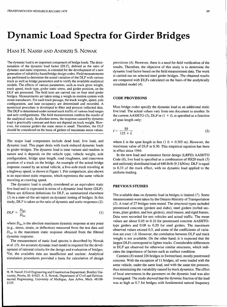
TRANSPORTATION RESEARCH RECORD 1476 69
Dynamic Load Spectra for Girder Bridges
HANI H. NASSIF AND ANDRZEJ S. NOWAK
The dynamic load is an important component of bridge loads. The determination of the dynamic load factor (DLF), defined as the ratio of dynamic and static responses, is essential for the development of a new generation of reliability-based bridge design codes. Field measurements are performed to determine the actual variation of the DLF with various truck as well as bridge parameters and to verify the available analytical models. The effects of various parameters, such as truck gross weight, truck speed, truck type, girder static stress, and girder position, on the DLF are presented. The field tests are carried out on four steel girder bridges. Measurements are taken using a weigh-in-motion system with strain transducers. For each truck passage, the truck weight, speed, axle configuration, and lane occupancy are determined and recorded .. A numerical procedure is devel_oped to filter and process collected data. The DLF is determined under normal truck traffic of various load ranges and axle configurations. The field measurements confirm the results of the analytical study. In absolute terms, the response caused by dynamic load is practically constant and does not depend on_ truck weight. However, for exterior girders the static stress is small. Therefore, the DLF should be considered on the basis of girders of maximum stress values.
The major load components include dead load, live load, and dynamic load. This paper deals with truck-induced dynamic loads in girder bridges. The dynamic load is time variant and random in nature and it depends on the vehicle type~ vehicle weight, axle configuration, bridge span length, road roughness, and transverse position of a truck on the bridge. An example of the actual bridge response caused by an actual vehicle, a five-axle truck traveling at a highway speed, is shown in Figure 1. For comparison, also shown is an equivalent static response, which represents the same vehicle traveling at crawling speed.
The dynamic load is usually considered as an equivalent static live load and is expressed in terms of a dynamic load factor (DLF). There are different definitions for DLF, as summarized elsewhere (1) in a state-of-the-art report on dynamic testing of bridges. In this s.tudy, DLF is taken as the ratio of dynamic and static responses (2):
DLF= Ddyn
Dstat (1)
where Ddyn is the absolute maximum dynamic response at any point (e.g., stress, strain, or deflection) measured from the test data and Dsiai is the maximum static response obtained from the filtered dynamic response.
The measurement of static load spectra is described by Nowak et al. (3). An accurate dynamic load model is required for the development of rational criteria for the design and evaluation of bridges. Yet, the available data are insufficient and unclear. Analytical simulation procedures provided a basis for calculation of design .
H. H. Nassif, Civil Engineering and Construction Department, Bradley University, Peoria, Ill. 61625. A. S. Nowak, Department of Civil and Environmental Engineering, University of Michigan, Ann Arbor, Mich. 48109-2125.
provisions (4). However, there is a need for field verification of the results. Therefore, the objective of this study is to determine the dynamic load factor based on the field measurement data. The work is carried out on selected steel girder bridges. The obtained results are compared with DLFs calculated on the basis of the analytically simulated model ( 4).
CODE PROVISIONS
Most bridge codes specify the dynamic load as an additional static live load. The actual values vary from one document to another. In the current AASHTO (5), DLF or (1 + /), is specified as a function of span length only:
50 /=---
125 + L (2)
where L is the span length in feet (1 ft = 0.305 m). However, the maximum value of DLF is 0.30. This empirical equation has been in effect since 1944.
In the new load and resistance factor design (LRFD) AASHTO Code (6), live load is specified as a combination of HS20 truck (5) and uniformly distributed load of 640 lb/ft (9.3 kN/m). DLF is equal to 0.33 of the truck effect, with no dynamic load applied to the uniform loading.
PREVIOUS STUDIES
The available data on dynamic load in bridges is limited (7). Some measurements were taken by the Ontario Ministry of Transportation (2). A total of 27 bridges were tested. The structural types included prestressed concrete (girders and slabs), steel girders (rolled sections, plate girders, and box girders), steel trusses, and rigid frames. Data were recorded for test vehicles and actual traffic. The mean values are about 0.05 to 0.10 for prestressed concrete AASHTOtype girders and 0.08 to 0.20 for steel girders. The maximum observed values exceed 0.5, and some of the coefficients of variation are over 1.0. However, the correlation between DLF and truck weight is not available. On the other hand, it is expected that the larg~st DLFs correspond to lighter trucks. Considerable differences in DLF ~e observed for otherwise similar structures, which indicates the importance of factors such as surface condition.
Cantieni (8) tested 226 bridges in Switzerland, mostly prestressed concrete. With the exception of 11 bridges, all were loaded with the same vehicle, under the same load, and with the same tire pressure, thus minimizing the variability caused by truck dynamics. The effect of local unevenness in the pavement on the dynamic load was also investigated. The study showed that the dynamic fraction of the loadwas as high as 0. 7 for bridges with fundamental natural frequency

70
30
25
al 20 ~ ,Ji 15 en f ... rn
10
5.0
0.0 0 0.2 0.4 0.6 0.8
Time. sec
5 Axle Truck Weight: 19.0 Mg
Speed : 104 km/hr
--Dynamic
-- ---Static
1.2 1.4 1.6
FIGURE 1. Dynamic and static response for Girder 3, Bridge 1, under a five-axle truck (1 MPa = 6.89 ksi; 1 km = 0.6 mi, 1Mg=1,814 lb).
between 2 and 4 Hz. However, as in the Ontario data (2), the static and dynamic loads were recorded separately, so that it is not possible now to determine the degree of correlation. It is also expected that the high values of DLF are associated with lighter vehicles.
O'Connor and Pritchard (9) found that the dynamic load is vehicle dependent and varies with the suspension geometry. They carried their tests on a short-span composite steel and concrete bridge in Australia. The results indicate that as the weight of the vehicle increases, the dynamic load decreases. Also, O'Connor and Chan (10) collected strain data and, using those records, determined DLFs ranging from -0.08 to + 1.32. As in the previous studies, the extreme values are associated with light trucks.
Most of the theoretical studies on vibration of beams under moving loads concentrated on modeling only one of the parameterseither the vehicle, bridge, or surface roughness. The vehicle was modeled as a constant force (11), one degree-of-freedom system (12), two degrees-of-freedom system, or more realistic complex systems (13). The bridge was modeled as either a continuous or discrete system (14). Discrete models can be in the form of simple beams, .simple beams with torsional degree of freedom, and orthotropic plates. The surface roughness was modeled using the so-called artificial bump on the approach method (13), and Honda and Kobori (14) used a random process to represent the random road profile as a Fourier series with random coefficients.
The development of a new LRFD code required a verification of the load model. In particular, there was a need for confirmation of the observation that the dynamic load factor decreases for heavier trucks and for multiple truck occurrence. Therefore, a computer procedure was developed previously (4) for simulation of the dynamic bridge behavior. The dynamic load was determined as a function of three major parameters: road surface roughness, bridge dynamics (frequency of vibration), and vehicle dynamics (suspension system). The bridge was modeled as a prismatic beam. Dynamic parameters of trucks were based on the available data. Road roughness was generated using the actual measurement records. The DLF was calculated in terms of deflections. It was found that the dynamic deflection is almost a constant, whereas static deflection is proportional to truck weight. Therefore, DLF decreases for heavier trucks. The
TRANSPORTATION RESEARCH RECORD 1476
simulations were carried out for single trucks and two trucks sideby-side. For two trucks, the DLF was smaller by about 50 percent compared with DLF for single trucks.
EXPERIMENTAL PROGRAM
The purpose of the experimental program is to measure the dynamic load amplification in simple-span steel girder bridges. Corresponding truck weights, in particular axle loads and axle spacings, are also recorded. The measurements are taken simultaneously by two systems: the weigh-in-motion (WIM) system (truck information and girder strains) and the dynamic system (accelerations) (15). The WIM system was developed by the bridge weigh systems. Its purpose is to measure and record all relevant truck information in addition to the strain response in each girder. The strain gauges are placed on lower flanges close to the position of the maximum moment. The dynamic system, developed by Krenz Electronics, is set up to measure accelerations simultaneously, and at the same location as, the strain gauges. Both systems are triggered by special tape switches, pasted to the pavement. The same tape switches are used to determine the truck speed, the number of axles, and axle spacings.
Four bridges are selected for the field tests. All of them are located in southeastern Michigan. The span lengths vary from 9 to 24 m (30 to 80 ft). The same procedure is used for all bridges, however, with a different equipment setup. All selected structures are multi-simple-span bridges with steel girders and concrete slabs. The basic design parameters include span length, girder spacing, slab thickness, and skewness. The basic parameters of the selected bridges are given in Table 1. Girders are labeled starting from the exterior girder in the right lane (Girder 1) to the exterior girder in the left lane (Girder 8).
The strain gauges are attached to bottom flanges of girders. The location of the strain gauge was 2 to 3 ft from midspan, depending on span length and access to the point of installation. The equipment is calibrated using trucks with known axle weights and spacings. The accuracy of calculation for axle ioads is within 20 percent and for gross vehicle weight (GVW) within 10 percent (within 5 percent for three and five axle trucks). The measurements are carried out for several days at each location.
A computer program is developed for the automated data processing. Each data file contained data from six or eight channels. Each record represents the passage of a truck over the bridge in either right or left lane. The data capturing starts when the truck crosses over the first tape switch, which is about 6 m (20 ft) from the bridge support in either lane. The tape switch signal is used to trigger the system and start collecting data from the accelerometers and strain transducers. The data collection is automatically stopped after the departure of the last truck axle from the bridge. However, this synchronization works for bridges with traffic intensity not higher than normal. On bridges with trucks of certain characteristics (e.g., heavy, 11 axles), the m~nual trigger permits a better control of the data acquisition system.
The strain records are smoothed and filtered using the widely used fast fourier transform (FFT) technique (16). The FFT procedure is utilized assuming that the measured strain-time (or acceleration-time data) can be represented as the sum of all contributions from all mode shapes. FFT is also used to determine the dominant frequencies as well as the cutoff frequency in the frequency domain. The cutoff frequency is best estimated, for each individual bridge,

Nassif and Nowak 71
TABLE 1. Parameters of the Tested Bridges
Brtdge I Location Span No. of
No. Girders
(m)
US-23/ 24.5 6
Huron River
2 M-14/ 16.0 8
N.Y.C. Rail Road
3 1-94/ 16.0 9
Jackson Road
4 1-94/ 10.5 10
Pierce Road
by minimizing the error in estimating the total energy under the power spectrum plot in the frequency domain. After eliminating the contribution of all modes (or frequencies) above the cutoff frequency in the frequency domain, inverse FFf is then performed to obtain the time-domain equivalent static response (referred to as static response). This process is performed on various truck strain records using a computer program that was developed on the basis of available numerical routines (15). The dynamic and static response are then plotted and compared to determine the DLF.
The WIM measurements provided data on truck ·weights., axle loads, axle configurations, and vehicle speeds. Most of the trucks traveled at about 90 km/hr (60 mph). The truck traffic was a mixture of mostly 5-axle vehicles with few very heavy 11-axle trucks. The GVW ranges were above the legal limits.
MEASURED DYNAMIC LOAD
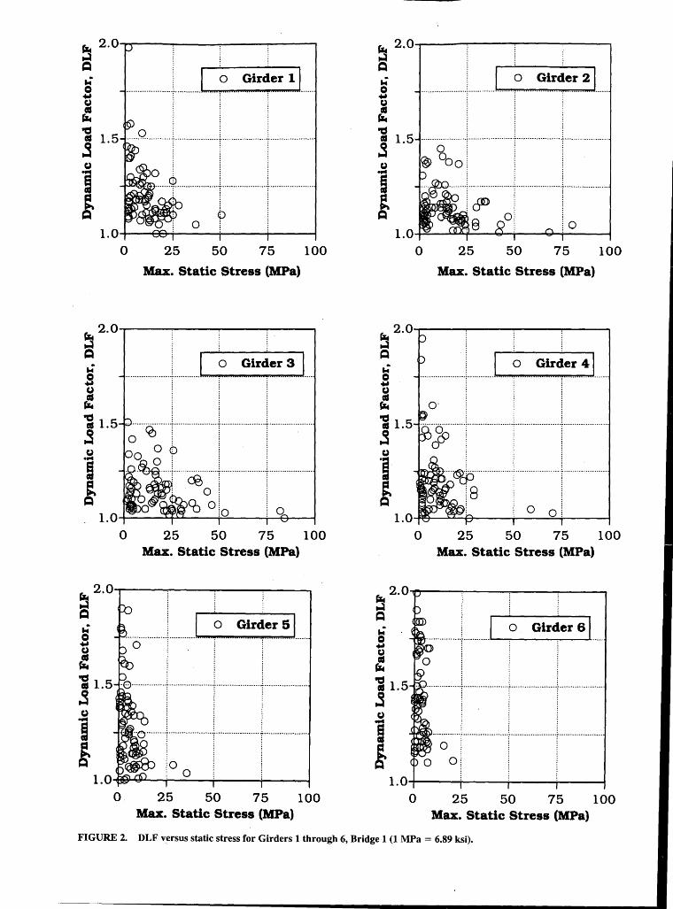
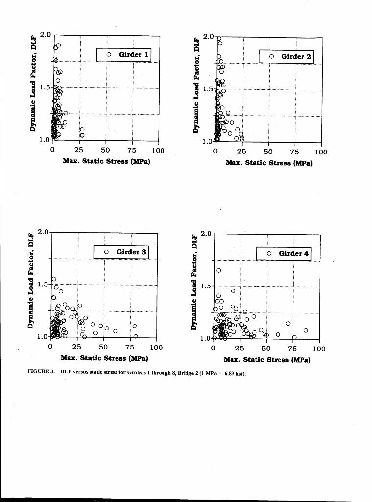
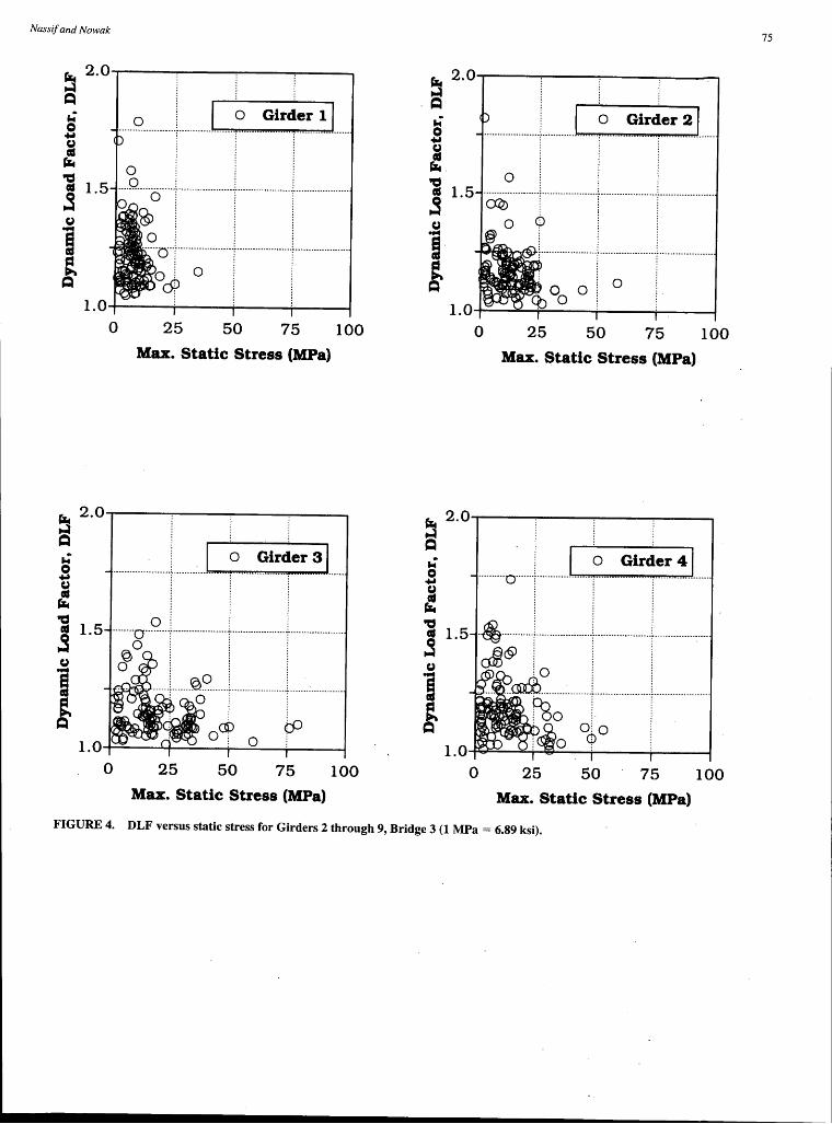
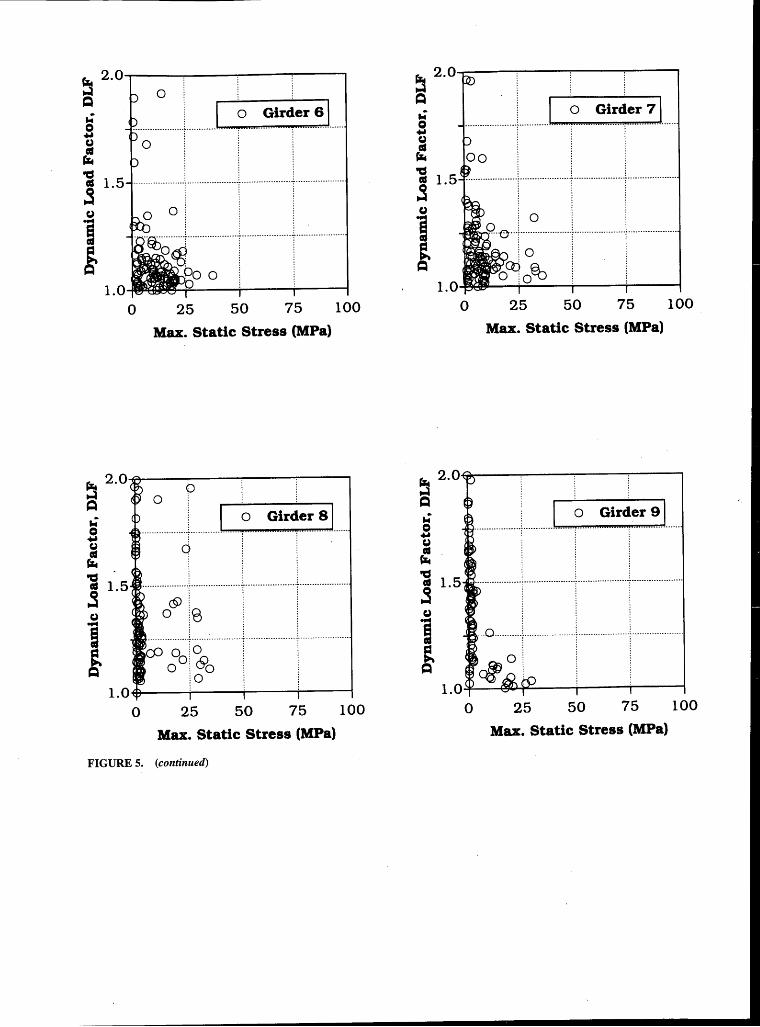
The measurements are carried out on four bridges listed in Table 1. Static and dynamic stress is determined for each girder. The resulting dynamic load factors (DLF) are plotted versus the static stress in each girder in Figures 2 through 5. The results are shown for a maximum of eight girders limited by the number of available data acquisition channels.
In general, DLF decreases as the static stress in each girder increases. However, the DLF is the ratio of dynamic and static stress, and static response varies from girder to girder, depending on the positions of the girder and truck. The variation in DLF with respect to static stress in each girder is shown in Figures 2 through 5. It is shown that the exterior girders exhibit small static stress (almost negligible), whereas the interior girders have much larger static stresses.
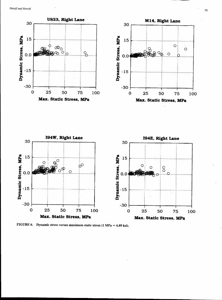
In general, the static stress is proportional to truck weight. However, the dynamic stress (maximum dynamic stress-maximum sta-
Girder Slab Brtdge Skew
Spacing Thickness Width
(m) (mm) (m)
1.90 190 11.0 14°
1.85 200 12.8 25°
l.70 190 14.5 25°
1.70 175 13.7 29°
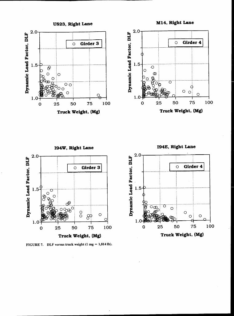
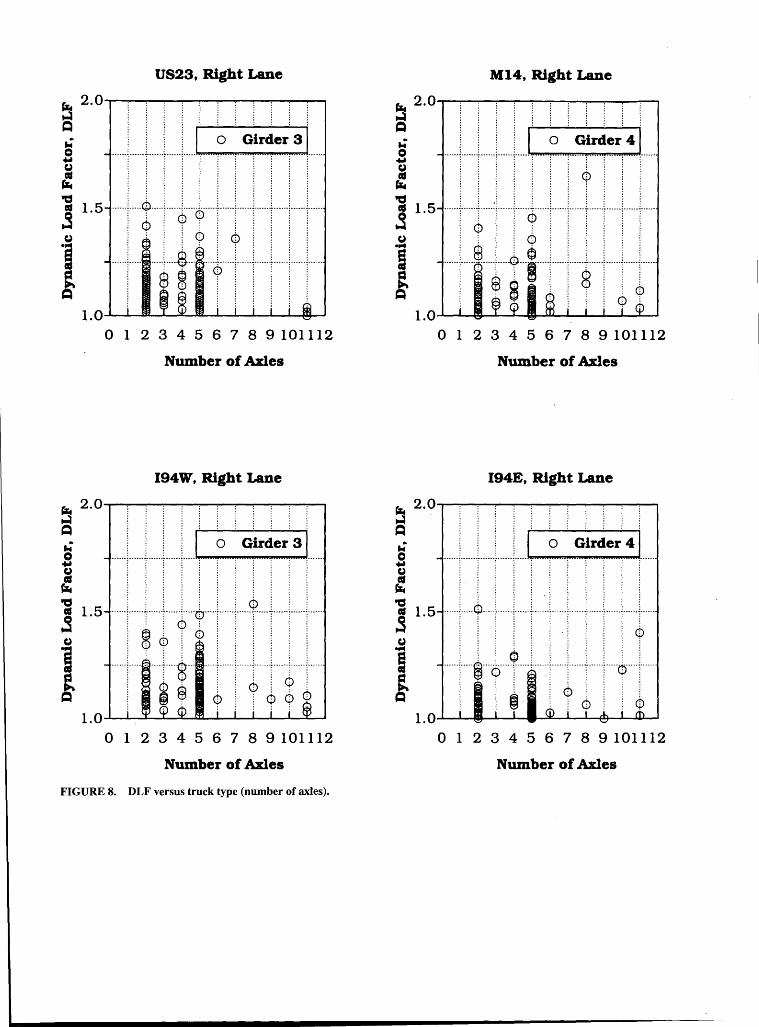
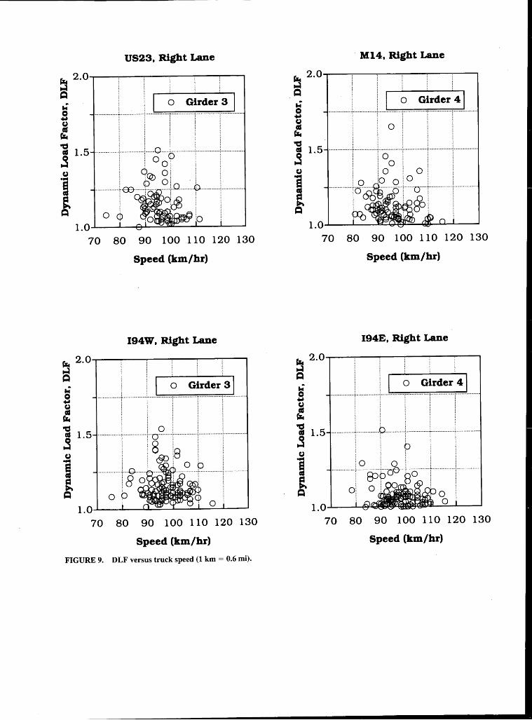
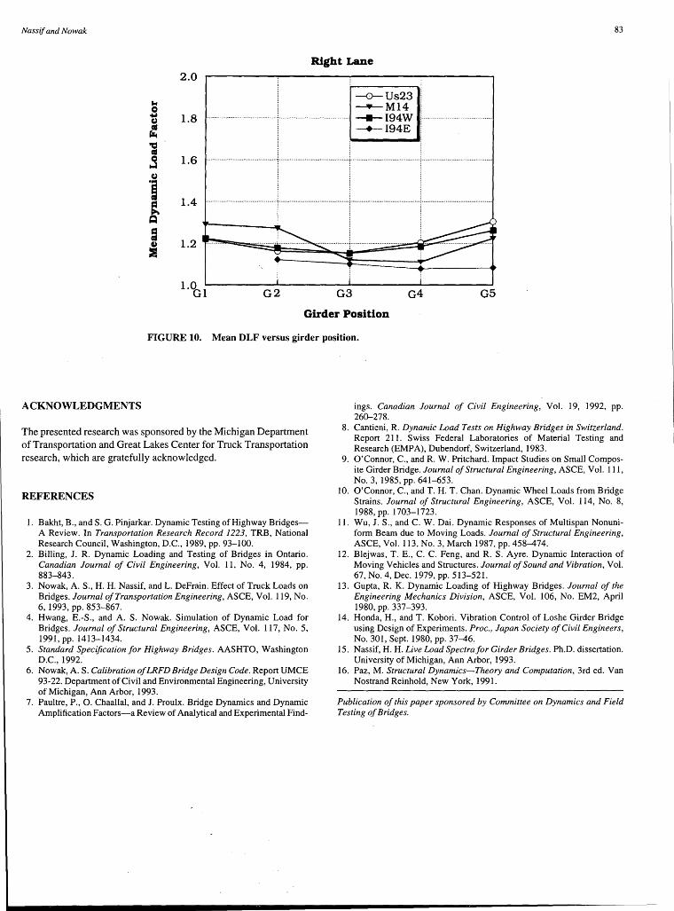
tic stress) is practically independent of truck weight (or static stress), as shown in Figure 6. Therefore, the dynamic load factor, DLF, decreases with increasing static stress or truck weight. The variation of DLF with truck parameters is shown in Figures 7 through 9. Results for each bridge are shown corresponding to the most loaded interior girder. Observations indicate that the DLF decreases as the GVW increases for all bridges (Figure 7). Observations also indicate that among all types of vehicles (excluding light-weight two-axle vehicles), four- and five-axle trucks cause the largest DLF values (Figure 8). Additionally, the DLF decreases with an increase in truck speed (Figure 9). Moreover, to represent the variation of DLF with girder position, the mean value of DLF, for right lane girders in each bridge, is plotted versus the girder position as shown in Figure 10. On average, the most loaded girders (Girders 3 and 4) will have values of DLF below 1.20.
CONCLUSIONS
The dynamic loads under a normal highway traffic are measured for selected steel girder bridges. For each truck, the measured parameters include: axle loads, axle spacings, speed, strain record, and acceleration record. A numerical procedure is developed for data processing, filtering, and smoothing. The DLF is calculated using strain records.
Observations indicate that the dynamic component of stress (i.e., dynamic increment) is practically independent of static component. Therefore, DLF decreases with increased static stress. For very heavy trucks, DLF does not exceed the theoretical results (4).
Larger values of DLF are observed in exterior girders; however, this is because of a relatively smaller static load effect. Values of DLF should be based on those obtained from the most loaded interior girders.
~ 2.0
a H•···H••·········l·······J
Q~ r· ··- . -· .
6 : ·-·····r···················-r···············--···-r·······-············
0 t ) 1. 0-+--~..;.-----;--__...----1
~ 2.0 ~
= ..;-s i .., as 1.5 .3 u .... ~ e. = 1.0
~ 2.0 ~ =
0 25 50 75 100
Max. Static Stress {MPa)
m•m m•,•HmJ 0 Girder 3
I. ...
0 25 50 75 100 Max. Static Stress {MPa)
mom HH'H• .m .. 0 (Hrder 5 L
·O··--·----------·[---------------·--·-f·--·-------------·--f--------------···-··
o·i· .. L .... - ...... . ! I I
i.o~~:..-.....,__;;.___,,___--i---~
0. 25 50 75 100 Max. Static Stress (MPa)
~ 2.0----....--------.-----, ..:a Q k 0 .. : 1 .3 u
1 &
mmHHmH!mm JHm~ ~irde~ 2 L
1. o~-~~__...,.,..__. _ ___..,~----1 0 25 50 75 100
Max. Static Stress {MPa)
~ 2.0 ..:a Q
um mm ••ml•HH HL H 0 Girde~ ~J... ...
--··@cfs··-·----------····j···------------------1--------------------
-~ :8 : : ...,.., HU...,-... 1 1 ~
i ! o oi L o~-....._R-----r--.::::...r----1
0 25 50 75 100 Max. Static Stress {MPa)
~ 2.0
~ um.mJH J 0 Girder 6 L ~ 0 i
] 1.5 . . ·: .. , .. t
1 ... L ... L .. -- .. & 0 : ! :
: : :
o! 1 1
1. 0-'----..... : __ ..... : ____ : __ -.I
0 25 50 75 100 Max. Static Stress (MPa)
FIGURE 2. DLF ~ersus static stress for Girders 1through6, Bridge 1 (1 MPa = 6.89 ksi).
. o Girder 11
lo : : !o ! !
1.0~1....-~~·~~~·---~~~· ~~-I
0 25 50 75 100 Max. Static Stress (MPa)
~ 2.0 ...:; Q
mmm• ·+·m•L .. Q Girder ~L . . .
·0~·-··········:·····················r·····················r····················
j ! i
... i<U~·~···· +·· -!~ o oi0 lo
1.0 0
i 0 : 0 i
25 50 75
Max. Static Stress (MPa)
100
~ 2.0---~~....,......~~....,......~~--~~~ ...:; - 0
Q ................ , .......... J ..... o .... ~irder.. 2 J. ... .
··a····-·········t·····················t·····················~····················
l l I 0 ! i ! ·····-·----- ... ~-- ... ·····---------- ··;·-· ------ ·····-···· -·:-··· ...... --- . ---- .. .
0 ! i i
o 01 I I o~ 1 :
.; c .... u al ~ ~
1.5 al .s u .... ~ &
1.0 0 25 50 75 100
Max. Static Stress (MPa)
~ 2.0 ...:; Q .; c .... u r: ~
1.5 al .s ~ :·[ 'm.: :i:e.r:J
0 ! ! ! 0 : :
u .... ~ &
00 j j . 0 Cbl l l
--~······~·~··a-···-···-t--··-··--··-·······t···-···-···-·····--. l Ol
o~ 0 i o l.o~~~-r--1.;;1::;,__....;.....~~-4-"-~~~
0 25 50 75 100
Max. Static Stress (MPa)
FIGURE 3. DLF versus static stress for Girders 1through8, Bridge 2 (1 MPa = 6.89 ksi).

1.0 ......... ---------------0 25 50 75 100
Max. Static Stress (MPa) Max. StaUc Stress (MPa)
0@ i I ~ Girder s j
omUUU! umu m 'mm•• mm WUu:UU : :
0 i.o~--.,__ _ ___. __ ------~
0 25 50 75 100 0 25 50 75 100
Max. Static Stress (MPa) Max. Static Stress (MPa)
FIGURE 3. (continuetf)
Nassif and Nowak 75
0 i I o Girder i j mmmHHmm! HHu mmr .. • •• U'umm H ..
0 i 0..... ' '.
! j o Girder 2 j
:~:Hr H~ :1mmum: :m ::
0 j ······o··!·····················i·····················i····················
: : :
oJ o I I 1. 0-+----...pi __ ......... i __ __.,.l ----1
0 6 i
! j
-4w!1f<ai~@~---·················-~---··················~---················-: :
o I o 1. O-+---=--....-..----r-----r-------1
0 25 50 75 100 0 25 50 75 100 Max. Static Stress (MPa) Max. Static Stress (MPa)
~ 2.0
a o Girde~ ~L ... : j o Girder 41
··········o·······r·····················!········--··········!················
0 1. o....,_;:..::~---1'-'-_;:;_-......,_--=---r------1
' '
~ ! i i . .s-~---···t·····················t·······-·············t··············-~---·· (fll)t;:;' : : :
io i i ~ : :
. .... ... P3-~---·-·····-r--··················-r--·················· : al 0 :
~ .......... CH7'.&J._...., 0 0 : 1.0 : :
0 25 50 75 100 0 25 50 75 100 Max. Static Stress (MPa) Max. Static Stress (MPa)
FIGURE 4. DLF versus static stress for Girders 2 through 9, Bridge 3 (1 MPa = 6.89 ksi).

~ 2.0...,..---.,.......--,,_..----:-----i
a H~lrder ~L
1.0-Fi-~~....,_ __ ,__ _ ___., __ --4
0 25 50 75 100
Max. Static Stress (MPa)
~ 2.0....,._--...----------. ~ Q
o Girder 71 ..
l \ I 1. 0-+""'-__ ....,_ __ ,___----;. __ --1
0 25 50 75 100
Max. Static Stress (MPa)
FIGURE 4. (continued)
~ 2. 0......---.----":"--------.
a 0
.: s i ] 1.5
1 ~
1. o...._ __ ..__ _ ___., __ --;..--~
~ 2.0
Q
0 25 50 75 100
Max. Static Stress (MPa)
I I 0 Girder s} Hmm !HH ........ ,.. . i .. HUH:
- ------------------:------------------·--!·------···--------·--r--·-----·-·------··--
--- --- ... ---. ---- "!" ---- ---- --- ---- -- -~ -~- --- -- -. -.. --------- ·:- -- ---- --- -.. ---- -- -
1. 0-+-------------T----P---'""'"1
0 25 50 75 100
Max. Static Stress (MPa)

~ 2.0 ~ Q ... 0 ~ u r:
'tS 1.5 • .3
u .... D ~
1.0
~ 2.0 ~ Q
0
1.0 0
25 50 75 100 Max. Static Stress (MPa)
01
25 50 75 100 Max. Static Stress -(MPa)
~ 2.0--~~.....-~~....,-~~--~~~ ~ i nnmnmlmnnJm~n ~er~Ln
]. 1.5 ····················!~··············!··················-···················· u 0 i i j ogf ,. ·~··· i io : : .... '0 0' j
1.0 0
~ 2.0 ~ Q ... 0 ~ c.> r:
'tS • .3 u .... m ~ Q
1.5
1.0 0
25 50 75 100 Max. Static Stress (MPa)
0 ~i~~.r.-~lm
lo : : :
o T ~ L ,
Oj .
25 50 75 100 Max. Static Stress (MPa)
FIGURE 5. DLF versus static stress for Girders 2 through 10, Bridge 4 (1 MPa = 6.89 ksi).
~ 2.0 t.J 0 Q .: 0 .... u «I
f;I;.
~ 1.5 as
.3 u .... ! ~
1.0 0 25 50 75 100
Max. Static Stress (MPa) Max. Static Stress (MPa)
i 2,0 n~mmJmJmm~ nGirde~~L ~ 9
·······-···········~----·-···-··········T··················-·t·······-············
o'§) :e : : ~ l j
............ ········~·· ........ ········ ···[ ··· ............... ···f ............. ·······
-----·······-····:. ..................... :. .................... ..:.. ................... . :0 :
cP oo: ,C) :
o : cro : :o l 1.0~--+-: ---+--_ ..... : __ --I i.o~-~+L-----i---+----i
0 25 50 75 100 0 25 50 75 100
Max. Static Stress (MPa) Max. Static Stress (MPa)
FIGURE 5. (continuetf)
Nassif and Nowak 79
30 --~~~~~~~~~~~ ....... US23, Right Lane
30 ...-~~.....--~~~.--~-,-~~--. Ml4, Right Lane
' 15 -------------·-··-·t····-·-----·-··--·--·j·--------···-·------1-----------··-------
ri ? (j))o I I :J JllfiQ•M· ~.Q) o lo i o !: 0.0
UJ u .... a Cd -15
~
~ 15 -------····---··-·+··-····-····--·-··+--····-··········-+·-·-···--···-······ 2 l i o: ri ii i i 0 i 0.0 ~-~-~g b .
i -15 • · 1 ··r i . -30 I I I
-30 1--~~-P-~~---~~---~~~
0 25 50 75 100 0 25 50 75 100 ·Max. Static Stress, MPa Max. Static Stress, MPa
30 194W, Right Lane
30 194E, Right Lane
------- --- --- --- -- -~ ------ --- --- ---------r--- --- -------· -- -----r------- ---- ---------
o: :;:. o ;g I Ma .. 0 .+-·-······o-···-···+·········-·--·······
' 11 ·
l! 15 :e ri en e o.o .....,
UJ u .... ~ -15
~
al 15 ~ :s
ri fl) I) !: 0.0 UJ u
1-15 ~ = : : -30 -30
0 25 50 75 100 0 25 50 75 100 Max. Static Stress, MPa Max. Static Stress, MPa
FIGURE 6. Dynamic stress versus maximum static stress (1 MPa = 6.89 ksi).
US23, Right Lane Ml4, Right Lane
~ 2.0 ~ Q .; 0 .... ~ ~
~ 2.0 ..:a Q .; 0 .... ~ ~
o Girder ~ _ J __ _ .. nm•H ...... mj 0 Girder 4J..m
"d 1.5 as
.3 u
1 e. Q
1.0
"d 1.5 as
.3 u .... m
& 1.0 0
. . . --·----··-~0-···-·r···-·---------------·r··---·---------·--·--r··------·-----------
(Q) : . :
Q.~6(; o'· . L. : l 0
~'lo.Mnml"~: : 0 0 : ; : : 0
0 25 50 75 100 0 25 50 75 100
Truck Weight, (Mg) Truck Weight, (Mg)
194W, Right Lane 194E, Right Lane
25 5{) 75 100 0 25 50 75 100
Truck Weight, (Mg) Truck Weight, (Mg)
FIGURE 7. DLF versus truck weight (1 mg = 1,814 lb).
~ 2.0 ~ Q ..; 0 .... g at
I&. 't:S
1.5 at
.3 u .... ~ &
1.0
(';I:. 2.0 ~ Q ..; 0 .... g at
f;r. 't:S
1.5 at
.3 u
i &
0 1
US23, Right Lane
2 3 4 5 6 7 8 9 101112
Number of Axles
194W, Right Lane
1. 0 _.__.___.__...._ ............. w...-..i__....__.__,___,___.___.
0 1 2 3 4 5 6 7 8 9 101112
Number of Axles
FIGURE 8. DLF versus truck type (number of axles).
Ml4, Right Lane
0 1 2 3 4 5 6 7 8 9 101112
Number of Axles
194E, Right Lane
f.o [ l ' i If o ! Girder4j
! 1. 5 ::::[LI:::r::1::::1.::::1.::: .. _::.1 ... :::1:.J::: .3 : : ! ! ! : . : i i : cb u i i : : i i i i : : :
] ······,·····~···9··f .... l ..... !·············-·····f ···o····r·····
& : : ~ : ¢ : ! ! l i 6 : i 0 i i ~
I. o_.__"""'--411it-_..._........,.~___._---+"+__,_ __ __.
0 1 2 3 4 5 6 7 8 9 101112
Number of Axles
US23, Right Lane
\ ~85 : : 0 Q
1. 0..L..--..1....-~.L....-:~L-~---1--......I
70 80 90 100 110 120 130
Speed (km/hr)
I94W, Right Lane
~ 2.0 t.J Q
.: 0 .... u ~ 'tS as .3 u .... ~ ~ Q
n mu nL nmjnnmnm ~n m~i~~~~'~L
1.5 : ' 0 ' ! ' ·············;·············1··o········;·············T·-···········i·············
! \ 8 :8 \ \ ;oJ.~! ?P ; :8 o· : : : l : ' '. 1
0 o.: cD i . 0: l.O_,__--'--____i,..~;..........11.....--..-.a.---'----'
70 80 90 100 110 120 130
Speed (km/hr)
FIGURE 9. DLF versus truck speed (1 km= 0.6 mi).
Ml4, Right Lane
~ 2.0....---.....----.----------. t.J Q
194E, Right Lane
1.0 70 80 90 100 110 120 130
Speed (km/hr)
Nassif and Nowak
2.0
r.c 0
Right Lane
--o--Us23 _._Ml4
83
..., 1.8 u t··············································,·················································I ~194\V•>·············································I
r: -+-194E
"Cl as .3 1.6 u
"! 1.4
~ ~
= 1.2 t) :s
l.C~H G2 G3 G4 G5
Girder Position
FIGURE 10. Mean DLF versus girder position.
ACKNOWLEDGMENTS
The presented research was sponsored by the Michigan Department of Transportation and Great Lakes Center for Truck Transportation research, which are gratefully acknowledged.
REFERENCES
I. Bakht, B., and S. G. Pinjarkar. Dynamic Testing of Highway BridgesA Review. In Transportation Research Record 1223, TRB, National Research Council, Washington, D.C., 1989, pp. 93-100.
2. Billing, J. R. Dynamic Loading and Testing of Bridges in Ontario. Canadian Journal of Civil Engineering, Vol. 11, No. 4, 1984, pp. 883-843.
3. Nowak, A. S., H. H. Nassif, and L. DeFrain. Effect of Truck Loads on Bridges. Journal of Transportation Engineering, ASCE, Vol. 119, No. 6, 1993,pp. 853-867.
4. Hwang, E.-S., and A. S. Nowak. Simulation of Dynamic Load for Bridges. Journal of Structural Engineering, ASCE, Vol. 117, No. 5, 1991, pp. 1413-1434.
5. Standard Specification for Highway Bridges. AASHTO, Washington D.C., 1992.
6. Nowak, A. S. Calibration of LRFD Bridge Design Code. Report UMCE 93-22. Department of Civil and Environmental Engineering, University of Michigan, Ann Arbor, 1993.
7. Paultre, P., 0. Chaallal, and J. Proulx. Bridge Dynamics and Dynamic Amplification Factors-a Review of Analytical and Experimental Find-
ings. Canadian Journal of Civil Engineering, Vol. 19, 1992, pp. 260-278.
8. Cantieni, R. Dynamic Load Tests on Highway Bridges in Switzerland. Report 211. Swiss Federal Laboratories of Material Testing and Research (EMPA), Dubendorf, Switzerland, 1983.
9. O'Connor, C., and R. W. Pritchard. Impact Studies on Small Composite Girder Bridge. Journal of Structural Engineering, ASCE, Vol. 111, No.3, 1985,pp.641-653.
10. O'Connor, C., and T. H. T. Chan. Dynamic Wheel Loads from Bridge Strains. Journal of Structural Engineering, ASCE, Vol. 114, No. 8, 1988,pp. 1703-1723.
11. Wu, J. S., and C. W. Dai. Dynamic Responses of Multispan Nonuniform Beam due to Moving Loads. Journal of Structural Engineering, ASCE, Vol. 113, No. 3, March 1987, pp. 458-474.
12. Blejwas, T. E., C. C. Feng, and R. S. Ayre. Dynamic Interaction of Moving Vehicles and Structures. Journal of Sound and Vibration, Vol. 67, No. 4, Dec. 1979, pp. 513-521.
13. Gupta, R. K. Dynamic Loading of Highway Bridges. Journal of the Engineering Mechanics Division, ASCE, Vol. 106, No. EM2, April 1980,pp. 337-393.
14. Honda, H., and T. Kobori. Vibration Control of Loshe Girder Bridge using Design of Experiments. Proc., Japan Society of Civil Engineers, No. 301, Sept. 1980, pp. 37-46.
15. Nassif, H. H. Live Load Spectra for Girder Bridges. Ph.D. dissertation. University of Michigan, Ann Arbor, 1993.
16. Paz, M. Structural Dynamics-Theory and Computation, 3rd ed. Van Nostrand Reinhold, New York, 1991.
Publication of this paper sponsored by Committee on Dynamics and Field Testing of Bridges.