Dynamic Load Balancing for Compressible Multiphase Turbulenceics2018.ict.ac.cn/essay/ics18-final62.pdf · Dynamic load balancing for scientific applications that consist of coupled

Dynamic Load Balancing for Compressible MultiphaseTurbulence

Keke Zhai

CISE, University of Florida

[email protected]

Tania Banerjee


[email protected]

David Zwick

MAE, University of Florida

[email protected]

Jason Hackl

MAE, University of Florida

[email protected]

Sanjay Ranka


[email protected]

ABSTRACTCMT-nek is a new scientific application for performing high fidelity

predictive simulations of particle laden explosively dispersed tur-

bulent flows. CMT-nek involves detailed simulations, is compute

intensive and is targeted to be deployed on exascale platforms. The

moving particles are the main source of load imbalance as the ap-

plication is executed on parallel processors. In a demonstration

problem, all the particles are initially in a closed container until a

detonation occurs and the particles move apart. If all processors

get an equal share of the fluid domain, then only some of the pro-

cessors get sections of the domain that are initially laden with

particles, leading to disparate load on the processors. In order to

eliminate load imbalance in different processors and to speedup

the makespan, we present different load balancing algorithms for

CMT-nek on large scale multi-core platforms consisting of hundred

of thousands of cores. The detailed process of the load balancing

algorithms are presented. The performance of the different load

balancing algorithms are compared and the associated overheads

are analyzed. Evaluations on the application with and without load

balancing are conducted and these show that with load balancing,

simulation time becomes faster by a factor of up to 9.97.

KEYWORDSDynamic Load Balancing, Map, Remap, Parallel Computing

ACM Reference Format:Keke Zhai, Tania Banerjee, David Zwick, Jason Hackl, and Sanjay Ranka.

2018. Dynamic Load Balancing for Compressible Multiphase Turbulence . In

ICS ’18: International Conference on Supercomputing, June 12–15, 2018, Beijing,China, Jennifer B. Sartor, Theo D’Hondt, and Wolfgang De Meuter (Eds.).

ACM, NewYork, NY, USA, 10 pages. https://doi.org/10.1145/3205289.3205304

1 INTRODUCTIONFlows with compressible multiphase turbulence (CMT) are difficult

to accurately predict and simulate because of complexities of the

actual physical processes involved. CMT-nek [1] is a new scientific

application that solves the compressible Navier-Stokes equations

Permission to make digital or hard copies of all or part of this work for personal or

classroom use is granted without fee provided that copies are not made or distributed

for profit or commercial advantage and that copies bear this notice and the full citation

on the first page. Copyrights for components of this work owned by others than ACM

must be honored. Abstracting with credit is permitted. To copy otherwise, or republish,

to post on servers or to redistribute to lists, requires prior specific permission and/or a

fee. Request permissions from [email protected].

ICS ’18, June 12–15, 2018, Beijing, China© 2018 Association for Computing Machinery.

ACM ISBN 978-1-4503-5783-8/18/06. . . $15.00

https://doi.org/10.1145/3205289.3205304

for multiphase flows. This application is designed to perform high

fidelity, predictive simulations of particle laden explosively dis-

persed turbulent flows under conditions of extreme pressure and

temperature. The actual physical processes underlying explosive

dispersal are complex and cover a very wide range of temporal and

spatial scales. Therefore, the simulations require enormous com-

puting power and CMT-nek is expected to be deployed in petascale

and exascale supercomputers.

CMT-nek leverages the code setup and data structures used in

Nek5000 which is an open source spectral element based com-

putational fluid dynamics code developed at Argonne National

Laboratory for simulating unsteady incompressible fluid flow with

thermal and passive scalar transport [2–4]. Nek5000 is a highly

scalable code, with demonstrated strong scaling to over a million

MPI ranks on ALCF BG/QMira. Nek5000 is, however, limited to low

speed flows by its formulation and discretization. Further, Nek5000

does not simulate particle laden flows. As a simulation workhorse,

CMT-nek is expected to facilitate fundamental breakthroughs and

development of better (physics-informed) models and closures for

compressible multiphase turbulence.

Nek5000 uses a static load balancing strategy, where the domain

is first partitioned into spectral elements. The domain partitioner

uses a recursive spectral bisection algorithm [5] and arranges the

resulting spectral elements in a one-dimensional array preserving

spatial locality. The one-dimensional array of spectral elements is

then equally divided among the processors. CMT-nek, on the other

hand, has a dynamic load balancing strategy. Firstly, CMT-nek esti-

mates the ratio of computational load between particles and fluid.

Then, the total computational load on each spectral element is cal-

culated and finally, the one-dimensional array of spectral elements

is partitioned, and elements are distributed to the processors so that

the computational load is evenly distributed. Thus, if the particles

are clustered in an area of the domain at the start of simulation,

then processors receiving elements from that area will be assigned

fewer elements compared to processors receiving elements outside

that area. As the particles begin to spread out, the current element

to processor assignment becomes sub-optimal degrading perfor-

mance and requiring a fresh element to processor assignment. In

contrast to Nek5000, CMT-nek can perform a reassignment.

Dynamic load balancing for scientific applications that consist

of coupled data structures is a challenging problem [6]. In this

paper, we showcase the improvement in performance of CMT-nek

(with moving particles and multiple coupled data structures) upon

using dynamic load balancing, with minimal overhead added due

https://doi.org/10.1145/3205289.3205304

https://doi.org/10.1145/3205289.3205304

ICS ’18, June 12–15, 2018, Beijing, China Keke Zhai, Tania Banerjee, David Zwick, Jason Hackl, and Sanjay Ranka

to the load balancing step itself. The application has a potential of

scaling to millions of MPI ranks in the future and load balancing

enhances its scalability. This is the type of scaling that is required for

achieving high performance on next generation exascale machines.

The load balancing techniques presented here may be applied to

a broad class of mesh-based or otherwise multidomain numerical

solvers of partial differential equations.

We developed three different algorithms for load balancing based

on centralized, distributed and hybrid approaches, respectively,

to distribute the computational load among processors. A pre-

processing step uses an architecture independent re-ordering strat-

egy to organize the load as a one-dimensional array [5] of spec-

tral elements with particles while preserving spatial locality. The

particles are mapped to the same processor that process the cor-

responding spectral elements containing these particles. The load

balancing algorithm speeds up CMT-nek by a factor of up to 9.97.

On an Intel Broadwell platform, the overhead of the hybrid load

balancing algorithm was only 1.82 times the cost of each iteration

for 65, 520MPI ranks, whereas on a BG/Q platform, the overhead

of the distributed load balancing algorithm was only 2.33 times the

computational cost of each iteration for 393, 216 MPI ranks. Given

that load balancing is performed every several hundred to several

thousand iterations, the load balancing overhead is negligible.

We also developed an algorithm to automatically initiate a load

balancing step as the application is running. This relieves the user

from having to specify a fixed interval when load balancing should

be triggered. We show that in one case this improves the overall

time by about 9.4% compared to a fixed load balancing approach

where a load balancing interval is specified by the user.

The rest of the paper is organized as follows. Section 2 presents

the related load balancing literature and how our work differs

from existing work. Section 3 gives a brief background of CMT-

nek. Section 4 presents our load balancing strategies. Experimental

results and conclusions are given in Sections 5 and 6, respectively.

2 RELATEDWORKDynamic load balancing has been researched extensively in various

other applications which require high performance computing. For

example, Lieber et al. [7] decouple the cloud scheme from the static

partitioning of the atmospheric model. Essentially, the cloud data

are managed by a new, highly scalable framework, that supports

dynamic load balancing. Due to the presence of tightly coupled data

structures of fluid and particles, CMT-nek cannot use that strategy

of creating a specialized framework for particles.

Menon et al. [8] present an adaptive load-balancing strategy

where the application monitors and decides the right time to trigger

a load-balancing scheme. While their work focuses specifically on

automatically triggering load balancing, in this work, we developed

a comprehensive load-balancing strategy for a real application,

which includes an automatic load balancer. The method used in

our automatic load balancer determines the slope of performance

degradation at runtime and based on this information the load

balancing period I is adjusted. Thus, unlike [8], our load-balancingperiod changes adaptively at runtime and hence is sensitive to

performance variations during simulation. Our method may also

trigger load balancing earlier in I if for some reason performance

degradation is greater than the overhead to load balance.

Another body of work involving load balancing is plasma-based

particle-in-cell (PIC) code [9–11]. Load balancing these codes presents

the same challenges as load balancing CMT-nek, due to the pres-

ence of tightly coupled data structures. CMT-nek is more complex

as it always models particle-particle interactions (four-way cou-

pling), whereas the PIC models such interactions only in certain

cases when a collision operator is implemented. Compared to the

work in [12] that uses the Hilbert-Peano curve to partition a do-

main, we use the spectral bisection method. Plimpton et al. [11] as

well as Nakashima et al. [13] perform a spatial decomposition as

in CMT-nek; however, the assignment of grid cells to processors is

static, whereas the number of particles is balanced out as part of

their load-balancing algorithm. In CMT-nek, on the other hand, the

processors owning the particles also own the grid cells (or spectral

elements, as we call them) and mapping of grid cells to processors

changes every time load balancing is done.

Pearce et al. [14] balance out particle-particle interactions instead

of the number of particles, in keeping with the fact that the work

done by a processor is proportional to the interactions computed.

This scheme benefits applications where the density of interactions

is nonuniform. CMT-nek does not only simulates particle-particle

interactions, but incurs additional computational load due to the in-

teractions between particles and fluid. Thus, the methods developed

by Pearce et al. may not readily be applied to CMT-nek.

Bhatele et al. [15] present a load-balancing approach suitable

for molecular dynamics applications that have a relatively uniform

density of molecules. The variation in particles density in CMT-nek

is much different from the situation considered in Bhatele et al.

The use of parallel k-d trees can improve the cost of particle-

particle interactions using techniques described in [16]. When the

number of cores in the platform is very large, the underlying many-

to-many communication between cores can be further optimized

by methods described in [17]. These will be considered in future.

3 BACKGROUND3.1 CMT-nekCMT-nek solves the three-dimensional Euler equations of fluid

dynamics in strong conservation-law form, using the discontinuous

Galerkin spectral element method [18] integrated by the third-order

total-variation-diminishing Runge-Kutta scheme of Gottlieb and

Shu [19]. Banerjee et al. [1] describe these steps in more detail, both

for CMT-nek and its proxy CMT-bone. We will now describe the

support for particles in CMT-nek.

3.2 Particles in CMT-nekThe particle algorithm follows the evolution of each particle in a

series of time steps. For a given time step, there are essentially three

phases:

Interpolation phase. Utilizing barycentric Lagrange interpola-

tion [20], fluid properties are interpolated from the grid points to

the location of a particle. This is done on an element-by-element

basis, meaning that only the Gauss-Lobatto grid points within the

spectral element in which the particle resides contribute to the fluid

properties at the particle location.

Equation solve phase. The force from the fluid on a particle is

evaluated using the previously interpolated fluid properties at the

particle location, along with time-varying and constant properties

of each particle, such as its velocity and mass. These forces are

Dynamic Load Balancing for Compressible Multiphase Turbulence ICS ’18, June 12–15, 2018, Beijing, China

P0–6 particles

P1–22 particles

P2–8 particles

1 2 10 7

5 6 11 9

3 4 12 8

1 2 3 4

5 6 7 8

9 10 11 12

Figure 1: An example of using spectral bisection method tomap a 2-D domain to a 1-D array and uniformly assign itselements to each processor.

Algorithm 1 Compute load on an element

Output: An array of computational loads of elements, indexed by

local element index

1: function compute_element_load

2: for each local element e do3: elementLoad[e] = particle load + fluid load

4: = number of particles in element + f luid_load▷ where f luid_load = average time to process an element /

average time to process a particle

5: end for6: end function

then used in explicit updates of the particle velocity and position

using the same third-order Runge-Kutta formulation for the time

integration as is used by the DGSEM solver for the fluid phase in

the Eulerian reference frame.

Movement phase. After the position of each particle is updated,

it is possible that it can spatially reside within a different spectral

element than it was in previously. If this occurs and the core that

holds the data of the previous spectral is different than the core

that holds the data of the new spectral element, the particle data is

transferred to the new core.

3.3 Parallelization in CMT-nekTo make an application scalable, the domain is partitioned, and

each processor gets a section of the domain [21, 22]. The mapping

process of spectral elements to processors may be decomposed into

three main stages:

(1) Transforming the 3-D distribution of elements in the fluid

domain to an architecture independent 1-D array of elements

while maintaining spatial locality [23]

(2) Partitioning the 1-D element array

(3) Mapping the element partitions to the processors

CMT-nek uses a recursive spectral bisectionmethod [5, 24] to create

the 1-D element array at first , which are then partitioned such that

each processor gets an equal number of elements. The particles

contained in an element are then assigned to the processor to which

the element is mapped. Figure 1 shows an example where a 1-D

element array is created from elements in a 2-D fluid domain and

partitioned uniformly by CMT-nek, irrespective of the number

of particles in an element. This partitioning strategy causes load

balancing issues, especially in the case of particle-laden explosively

driven flows, where billions of particles might be initially contained

in a small region of the overall domain.

Algorithm 2 Centralized load balancing algorithm

Output: A load balanced element to processor assignment

1: function recompute_partitions

2: for each processor Pi do3: call compute_element_load

4: send array elementLoad to Processor P05: end for6: P0 receives elementLoad from processors

7: P0 sorts elementLoad based on global element index

8: P0 computes prefix sum of elementLoad9: P0 stores the prefix sum in array pre f ix_sum10: call partition_load(pre f ix_sum, lenдth) to decide where

to chop the pre f ix_sum array and assign element→processor

map

11: P0 broadcasts the new element→processor map

12: return element→processor map

13: end function

4 LOAD BALANCING CMT-NEKIn this section we describe our load balancing strategy. Section 4.1

shows how the computational load on an element is determined for

the purposes of load balancing. Section 4.2 presents a centralized,

a distributed and a hybrid version of the domain repartitioning

algorithm. Section 4.3 presents an example that further clarifies the

steps in these algorithms. Section 4.4 describes the logistics of data

sharing between processors, and finally, Section 4.5 describes two

algorithms for triggering load balancing at runtime.

4.1 Determining computational load on aspectral element

Computational load on an element is quantified as the number of

particles present inside the element plus a baseline load for fluid

computation. The latter is considered to be about the same for any

element since fluid computations involve solving fluid properties at

each grid point in an element and all hexahedral spectral elements

have the same number of grid points. In fact, the load on each

element due to fluid computations isO(N 4), where N is the number

of grid points along one direction [25]. To ensure that particle load

does not dominate fluid load and vice versa, we represent fluid load

as a constant defined as the ratio of the average time it takes to

process a single element to the average time it takes to process a

single particle by running the application prior to enabling load

balancing. This constant is dependent on the platform and also on

problem parameters such as grid size. Algorithm 1 describes the

computation of relative load on an element. Once the computational

load for each element is determined, the next step is to repartition

the 1-D array of spectral elements as shown in Figure 1, which is

described in next section.

4.2 Repartitioning strategiesWe developed a centralized, a distributed and a hybrid algorithm

for repartitioning the 1-D array.

4.2.1 Centralized. The main theme of the centralized algorithm

is that all the processors send their total computational load to pro-

cessor P0. Processor P0 then computes the prefix sum of the load on

elements ordered according to their global IDs, partitions the prefix

sum array, uses the partitioning to create a new element→processor


Algorithm 3 Partition algorithm called by centralized load balanc-

ing algorithm

1: function partition_load(pre f ix_sum, lenдth) ▷

this function is called in Algorithm 2, lenдth is the number of

entries in the pre f ix_sum array

2: np = number of processors ▷ create np partitions of

element array as follows

3: lp = 0 ▷ position of last partitioning

4: for i = 1, np - 1 do5: threshold = i × pre f ix_sum(lenдth)/np6: iterate over pre f ix_sum and determine the

7: position p of the first sum that exceeds threshold8: consider pre f ix_sum entries at p and p − 1

9: d1 = distance(pre f ix_sum(p − 1), threshold)10: d2 = distance(pre f ix_sum(p), threshold)11: if d1 < d2 then12: include p − lp − 1 entries in current partition

13: lp = p − 1

14: else15: include p − lp entries in current partition

16: lp = p17: end if18: map elements in current partition to processor Pi−119: end for20: map elements in the last partition to the last processor

21: return element→ processor map

22: end function

mapM ′, and finally, broadcastsM ′

to all processors. This scheme is

presented in Algorithm 2 and the steps are traced using an example.

4.2.2 Distributed. The centralized load balancing has processor

P0 in the critical path that determines how fast the load balancing

may complete. In the distributed version, we remove this bottle-

neck and let each processor collaborate to have a local copy of the

prefix sum of the load. After that, each processor calculates a local

element→processor map. The processors share their local maps

which each processor composes to form a global element→processor

map. As a last step, each processor adjusts the mapping to guar-

antee that the number of elements assigned to a processor does

not exceed a maximum bound defined by the user by setting a

variable “lelt". The distributed load-balancing scheme is presented

in Algorithm 4 and the steps are traced using an example.

4.2.3 Hybrid. The hybrid load-balancing algorithm is a combi-

nation of the centralized and distributed algorithms. First, the pro-

cessors collaboratively create the local copy of the prefix sum and

each processor calculates a local element→processor map. Then,

each processor sends the local map to processor P0. P0 then ag-

gregates the data to create the global map. P0 also adjusts the

mapping to guarantee that the number of elements assigned to

a processor does not exceed “lelt". Finally, processor P0 broad-

casts the element→processor map,M ′, to all processors. In order

to save space, the hybrid algorithm is omitted here. However, it

is basically Lines 1-7 in Algorithm 4, Lines 1-20 in Algorithm 5,

sending element→processor map to processor P0, Line 22 in Algo-

rithm 5 executed on processor P0, and finally, broadcasting the newelement→processor map to all processors.

Algorithm 4 Distributed load balancing algorithm

Output: A load balanced element to processor assignment

1: for each processor Pi in parallel do2: call compute_element_load

3: compute pre f ix_sum for element load array of Pi4: loadsumi = sum of total load on P0, · · · , Pi−2, Pi−15: for each entry in pre f ix_sum array do6: add loadsumi to that entry

7: end for8: call partition_load_distributed(pre f ix_sum,nelдt ,lelt )9: end for

Processor P0 P1 P2

Initially, element load = particle load + fluid computation loadAdditionally, here for simplicity, load due to fluid computation is computed as:

total number of particles/total number of elements = 36/12 = 3

Hence, total element load is given by the following (Lines 2-5, Algorithm 1)

All processors send element load to processor P0.P0 sorts the loads based on global element id. Thus, processor P0 has (Line 7, Algorithm 2):

Local element id 1 2 3 4 1 2 3 4 1 2 3 4

Global element id 1 2 3 4 5 6 7 8 9 10 11 12

Particle load 0 3 1 2 5 5 7 5 4 0 4 0

Local element id 1 2 3 4 1 2 3 4 1 2 3 4


Element load 0+3

3+3

1+3

2+3

5+3

5+3

7+3

5+3

4+3

0+3

4+3

0+3


Element load 3 6 4 5 8 8 10 8 7 3 7 3

Figure 2: Centralized LB Step 1: Calculate element load arrayand send it to processor P04.3 An example illustrating the repartitioning

strategiesSuppose the fluid domain has been partitioned into 12 elements,

converted into 1-D array using the recursive spectral bisection

method, and that there are 36 particles placed in these elements,

as shown in Figure 1. Further suppose that there are 3 processors,

P0, P1 and P2. Initially, CMT-nek partitions the element array uni-

formly, so each processor gets 4 elements. This setup and the initial

element→processor assignment are shown in Figure 2. Using this

setup, the element load is calculated using Algorithm 1, where fluid

load is computed as 3.

Steps in centralized load balancing. In a centralized version,

all processors send their arrays of element load to a central proces-

sor P0 as shown in Figure 2. We use the underlying crystal router

mechanism in Nek5000 for this communication. Thus, by the end

of this step, the processor P0 has gathered the load for all elements

and have sorted them based on the global element ordering.

Figure 3 shows the second step in the centralized algorithm,

where P0 processes the element load information received. The

element load array stores the total computational load on elements

indexed by the global element index. Following that, processor P0computes its prefix sum, as well as a threshold load computed as

the total load divided by the number of processors. The threshold

load helps us to distribute the load as evenly as possible on the

processors. In our example, the threshold load is 72/3 = 24.

After a threshold value is calculated, processor P0 iterates overthe element load array and checks the point where the threshold is


Algorithm 5 Partition algorithm called by distributed load balanc-

ing algorithm

Input: Prefix sum of element load array, pre f ix_sumInput: Total number of elements in the application, nelдtInput: Maximum number of elements allowed on a processor, leltOutput: Element to processor mapping

1: function partition_load_distributed(pre f ix_sum, nelдt ,lelt ) ▷ This function is called in Algorithm 4 by processor Pi

2: np = number of processors

3: total_load = total number of particles + f luid_load ×nelдt4: loadavд = total_load/np ▷ Each processor should ideally

have loadavд load; first round of processor assignment:

5: e = local element index

6: for e = 0 to last_e do ▷ all elements in Pi7: processor [e] = (pre f ix_sum[e] - 1) / loadavд8: end for9: ▷ Second round of processor assignment to ensure the number

of elements assigned to a processor does not exceed limit lelt10: if Pi is neither the first nor the last processor then11: Send processor [last_e] to Pi+112: Recv processor [last_e] of Pi−113: Store received value in recvAssiдn14: else if current processor is the first processor then15: Send processor [last_e] to Pi+116: else if current processor is the last processor then17: Recv processor [last_e] of Pi−118: Store received value in recvAssiдn19: end if20: Using recvAssiдn when present, and processor [e] mapping

for all local elements, Pi creates a mapping of processor index

and element left boundary represented by the global element

index of first element assigned to the processor.

21: The processors callMPI_ALLGATHERV to gather this in-

formation and at the end of this step all processors have a

mapping of processor index and global element index of the

first element.

22: Pi checks if the number of elements assigned to processor

Pk ,k = 0, · · · ,np− 1, is bounded by lelt . If number of elements

assigned to processor Pk is greater than lelt , the right element

boundary for Pk is moved to left until the number of elements

in Pk is lelt . The number of elements in Pk+1 increases and thebound check is continued for processor Pk+1, Pk+2 and so on.

23: end function

reached or just exceeded.When that point is reached, two preceding

values in the element load array are evaluated to check where the

partition should be placed. In our example, the prefix sum values

for elements 4 and 5 (sum values of 18 and 26) are evaluated against

the threshold to determine the first position of partitioning. Since

24 − 18 = 6, whereas 26 − 24 = 2, element 5 is nearer to threshold

24, and therefore, the position of the first cut is in between the fifth

and sixth elements. In the meantime, “lelt" is also considered. If

the maximum number of elements in a processor has been reached

while the threshold position hasn’t, the partition is still placed here.

Since there are three processors, two cuts will be needed to create

three partitions. The nth cut to the load array will happen at a point

Processor P0

P0 calculates the prefix sum of element load (Line 8, Algorithm 2)

Compute the threshold load for partitioning prefix sum (Line 5, Algorithm 3):threshold interval = total load/number of precossors = 72/3 = 24

So cuts will be done for threshold loads of 24, 48

Candidates for first cut

First cut may happen between element 4 and 5, or between element 5 and 6Choose the one closest to the threshold (Line 6-17, Algorithm 3)Thus, cut happens between elements 5 and 6 since |18-24|= 6 and |26-24|=2

Hence, the partition is as follows:

Partition 1 Partition 2 Partition 3(Line 18, 20, Algorithm 3)

Partition 1 Partition 2 Partition 3

Global element id 1 2 3 4 5 6 7 8 9 10 11 12Element load 3 6 4 5 8 8 10 8 7 3 7 3

Global element id 1 2 3 4 5 6 7 8 9 10 11 12Prefix sum 3 9 13 18 26 34 44 52 59 62 69 72



Global element id 1 2 3 4 5 6 7 8 9 10 11 12Processor mapping 0 0 0 0 0 1 1 2 2 2 2 2

Figure 3: Centralized LB Step 2: Processor P0 determines newelement→processor mapping array based on the prefix sumof element loadProcessor P0 broadcasts new map (Line 11, Algorithm 2). At the end of load balancing anddata transfer, following is the elements distribution

Processor P0 P1 P2Local element id 1 2 3 4 5 1 2 1 2 3 4 5Global element id 1 2 3 4 5 6 7 8 9 10 11 12

Figure 4: Centralized LB Step 3: Every processor gets the newpartition after load balancing

Starting with the same example as for the centralized algorithm,each processor calculates the local prefix sum of element load (Line 3 in Algorithm 4):

Each processor retrieves the local prefix sum of the last element,

And calculate the exclusive prefix sum of all the processors (Line 4 in Algorithm 4):

Add the exclusive prefix sum back to the local prefix sum and each element get the global prefixsum (Lines 5-7 in Algorithm 4):

Local element id 1 2 3 4 1 2 3 4 1 2 3 4


Local Prefix Sum 3 9 13 18 8 16 26 34 7 10 17 20

Process P0 P1 P2

Last Prefix Sum 18 34 20

Process P0 P1 P2

Exclusive Prefix Sum 0 18 52

Local element id 1 2 3 4 1 2 3 4 1 2 3 4


Global Prefix Sum 3 9 13 18 26 34 44 52 59 62 69 72

Figure 5: Distributed LB Step 1: Calculate element load andthe global prefix sumwhere the load is close to threshold ×n. Thus, the threshold for thesecond cut is 24 × 2 = 48, and the second cut is made between the

seventh and eighth elements.


Each processor calculates the total load in this system (Line 3 in Algorithm 5):total load = total number of particles + fluid computation*total number of elements = 72

average load (Line 4 in Algorithm 5) = total load/number of processors = 24Processor mapping is calculated as (prefix sum-1)/average load (Lines 5-8 in Algorithm 5)

Each processor sends the last processor mapping to its next processor, and receives what issend from the previous processor (Lines 10-19 in Algorithm 5).

Each processor compares what it receives, and create the table that tracks the element thatis assigned to processor different from the previous element (Line 20 in Algorithm 5)

Concatenate these arrays to get the global array by each processor (Line 21 in Algorithm 5)

Based on the beginning positions, each processor checks the number of elements assignedto a processor such that it won’t exceed the maximum number of elements belonged toeach processor. Here lelt is not exceeded, so the final distribution is P0 owns elements from1-4, P1 owns elements from 5-7 and P2 owns elements from 8 -12.

Local element id 1 2 3 4 1 2 3 4 1 2 3 4


Processor mapping 0 0 0 0 1 1 1 2 2 2 2 2

Local element id 1 2 3 4 1 2 3 4 1 2 3 4


Processor mapping 0 0 0 0 1 1 1 2 2 2 2 2

Process P0 P1 P2Processor mapping 0 1 2

Beginning position 1 5 8

Process P0 P1 P2Processor mapping 0 1 2 0 1 2 0 1 2

Beginning position 1 5 8 1 5 8 1 5 8

Process P0 P1 P2Local element id 1 2 3 4 1 2 3 1 2 3 4 5


Figure 6: Distributed LB Step 2: Each processor comes upwith the new element→processor mapping array

Once the partitions are made, processor P0 creates the element

→ processor map. As shown in Figure 3, the first five elements

in the global 1-D array of elements are assigned to processor P0,the next two elements are assigned to processor P1 and the last

five elements are assigned to processor P2. This processor mapping

information, is with processor P0 only at this point. The mapping

array is then distributed by P0 to all the remaining processors.

This step concludes the centralized algorithm to remap elements to

processors as shown in Figure 4.

Steps in distributed load balancing. In the distributed ver-

sion, each processor computes the loads of elements assigned to it,

followed by a local prefix sum of the loads as shown in Figure 5. To

convert a local prefix sum to a global prefix sum, each processor

Pi needs to know the prefix sum of load residing on processor P0through processor Pi−1, which is also known as exclusive prefix

sum and implemented usingMPI_EXSCAN . By adding this exclu-

sive prefix sum to each entry of the local element load array, the

global prefix sum is obtained. This process is illustrated in Figure 5.

After obtaining the global prefix sum, each processor computes

element→processor mapping as shown in Figure 6. First, the to-

tal and average loads are calculated, which are 72 and 72/3 = 24,

respectively, in our example. Given that the processors are homo-

geneous, the element→processor mapping may be obtained by

simply dividing each global prefix sum (see Figure 5), less 1, by

the average load. At this point, each processor has a portion of the

new element→processor map, shown as “Processor mapping" in

Figure 6. Before making this new mapping the final one, we need

to guarantee that the number of elements assigned to a processor

does not exceed the maximum number defined by the user, that is

“lelt". A naive way to check it is using an all-to-all communication

to send and construct the entire global element→processor map at

each processor and adjusting the number of elements such that no

processor is assigned more than “lelt" elements.

Instead of sending the whole local element→processor map us-

ing the all-to-all communication as described above, the following

happens in our implementation: 1) each processor sends the proces-

sor mapping of the last element to the next processor, and receives

the data sent by the previous processor; and 2) each processor com-

pares data received from the previous processor with the processor

mapping for the first local element, to check if the processor map-

ping is the same or not. For example in Figure 6, the data received

by P2 is 2, and it is the same as the processor mapping assigned to

its first local element. Similarly, the data received by P1 is 0, whichis different from the processor number assigned to the first local

element in P1. This is significant because this information is used

by each processor to identify the global element index of the first

element assigned to any processor. For example, P2 can tell that

the element with global index 9 is not the first element assigned

to P2. Similarly, P1 can tell that the global element index of the

first elements assigned to P1 and P2 are 5 and 8, respectively. Then

each processor collectively has a list of the global element indices

of the first elements assigned to processors. Only this information

is then shared among the processors using all-to-all communica-

tion, and finally, all processors have a consolidated list of global

element indices of the first elements assigned to processors. Us-

ing this consolidated list, the processors then check the maximum

bounds on number of assigned elements (“lelt"), and fix it if violated.

This step concludes the distributed algorithm to remap elements to

processors as shown in Figure 6.

Steps in hybrid load balancing. In order to save space and

avoid repetition, the examples for the hybrid load balancing is omit-

ted here. It is the same as the distributed load-balancing examples

in Figure 5 and the first 3 steps in Figure 6. For the last but one

step in Figure 6, only processor P0 receives the processor map-

ping and adjusts the position to make the number of elements in

a processor within “lelt". Then, processor P0 broadcasts the newelement→processor map to all other processors.

Though in this example we started with uniform partitioning

and defined a repartitioning strategy, the same process may be

repeated as needed during the course of simulation whenever load

imbalances arise.

The readers would note that the element→processor mapping

arrays obtained using the centralized and distributed algorithms are

different. That is because for the centralized algorithm, processor

P0 has global information of each element’s load. While for the dis-

tributed algorithm, each processor only has local information. Thus,

the centralized algorithm can make better decisions with regard

to the element→processor mapping, compared to the distributed

algorithm. However, there is no performance bottleneck caused

by a single node in the distributed algorithm as in the centralized

algorithm. Thus, there is a trade-off between better decisions and

performance. The benefits of a hybrid load-balancing algorithm

would be explained in Section 5.3.

Transfer of elements and particles. The new element → pro-

cessor map is used by the processors to transfer elements and parti-

cles appropriately. For example, based on the new map obtained by


the centralized algorithm in our example, processor P1 would send

it’s first and last elements to processors P0 and P2, respectively. Theparticles contained in the domain of each transferred element are

transferred to the same respective destination processors.

So far we have described computational load balancing of ele-

ments and particles on processors. It is also important to consider

imbalances generated in the communication load. CMT-nek fol-

lows a discontinuous Galerkin scheme [1, 18] and hence is light

on communication. Communication is required for transferring

shared faces of elements residing on different processors. The origi-

nal CMT-nek distributes elements uniformly among the processors.

Hence, the number of faces to be shared is bounded implicitly.

On the other hand, load-balanced CMT-nek distributes elements

nonuniformly, which in the worst case, may result in an increase in

the communication overhead. The communication overhead for a

processor is upper bounded in the load-balanced code by specifying

a maximum limit on how many elements may be assigned to the

processor (“lelt"). Having such a limit also ensures that all elements

and data fit into processor memory.

4.4 Distributing Elements and ParticlesIn this section we will describe the details of how data is transferred

between processors. There are a large number of data structures

in CMT-nek that contain element and particle information. Some

of these data structures store static data while others store dy-

namic data. Static data include information such as the x , y and zcoordinates of each element, curvature on the curved faces, and

the boundary conditions. Dynamic data includes fluid and particle

properties that change during simulation. We follow two primary

strategies for information transfer.

4.4.1 Transferring data. Arrays storing the conserved variables

such as mass, energy, and the three components of momentum are

transferred. The transfer process consists of packing the arrays to be

transferred, transferring the packed array, and finally unpacking the

arrays received. We use the underlying crystal router in Nek5000

for transferring the packed data.

4.4.2 Reinitializing data. The data structures which store static

data are reinitialized. For this step, we initiate calls to existing

Nek5000 data initialization routines. This needed careful analysis

since some routines store the status of calls using static variables

local to the scope of the routines. We analyzed and updated such

routines employing static variables to reset the state of those vari-

ables when load balancing is done.

After load balancing is complete, a processor will start the next

time step, which involves the computation of field variables for all

elements, including the new ones that were received. For all our

tests we have diligently verified that the results of simulation has

the same accuracy as the original CMT-nek.

4.5 Triggering a load-balancing stepAs particles move during simulation, the original element→ proces-

sor mapping becomes suboptimal since the particle-heavy elements

with large computational load start getting lighter on particles as

the particles move apart. This motivates the need for a dynamic

load-balancing scheme, where load balancing may be triggered dur-

ing an ongoing simulation process. There are two main strategies

for triggering load balancing during simulation in CMT-nek. The

first is performing load balancing at specific intervals where the

Algorithm 6 Automatic load balancing

1: function Adaptive_load_balance ▷ is called after solver

step in the simulation.

2: threshold = 0.05; deдradation = 0.0

3: r_step = 0 ▷ Time step in which load balance happens

4: lb_time = time taken by load balancing algorithm

5: eval_interval = 100 ▷ Evaluate performance for these

many steps. An evaluation phase P starts one step after each

time load balance happens, P consists of eval_interval steps6: t1 = average time per time-step in P7: c1 = middle step in P ▷ c1 = 50, here, initially

8: cts = current-time-step

9: t2 = median of time per time-step among [cts − 2, cts]10: lb_once = false ▷ set to true after first call to load balance

11: if cts ∈ P then12: Update t1, c1; continue;13: else if lb_once == false then14: if (t2 − t1)/t1 > threshold then15: Perform load balance; calculate lb_time;16: reinit_itv = cts − c1; r_step = cts; lb_once = true

17: end if18: else if cts − r_step == 1 then19: rebal = sqrt(2 ∗ reinit_itv ∗ lb_time/(t2 − t1)) ▷ rebal

is the number of steps after which the next load balance would

theoretically happen

20: else21: deдradation = deдradation + (t2 − t1)22: if cts − r_step ≥ rebal | | deдradation > lb_time then23: Perform load balance; calculate lb_time24: reinit_itv = cts − r_step25: r_step = cts; deдradation = 0.0

26: end if27: end if28: end function

intervals are specified by the user. The second strategy is adaptive

load balancing, where no input is necessary from the user.

4.5.1 Fixed step load balancing. This type of load balancing

requires user input. For example, a load-balancing step may be

triggered after every k time steps, where k is specified by the user.

To set a reasonable value for k , the user should be aware of the

simulation details, such as the problem size, particle speed, duration

of a time step, and so on. The user may also run the simulation for

a certain time without load balancing to estimate k .

4.5.2 Adaptive load balancing. This type of load balancing is

performed automatically by the program, with no input from the

user. The details of the adaptive load-balance algorithm are pre-

sented in Algorithm 6. Before the adaptive load balancing strat-

egy is applied, there is one compulsory load-balancing step which

happens at the beginning after particles are initialized and placed

and before the start of simulation. After that, in Algorithm 6, a

load-balancing step happens whenever performance degrades by a

certain threshold (Line 14-17 in Algorithm 6). For subsequent load-

balancing steps, the application captures the cost of load balancing

(i.e., lb_time in Algorithm 6), the slope of performance degradation

(i.e., (t2 − t1)/reinit_itv in Algorithm 6). According to [8], we can


get the theoretical load-balancing interval (Line 19 in Algorithm

6). When this interval is reached, the load-balancing algorithm is

called. However, since the slope may be changing, we add another

criteria that is when the cost of load balancing is covered by the cost

caused by the increasing time-per-time-step, the load balancing is

called. After that, each time a load balancing is performed, the cost

of load balancing and the slope are updated and the new theoretical

load-balancing interval is calculated. Thus, load balancing is called

when either one of the two criteria is satisfied.

Note that, the value of threshold determines the time step when

load balancing happens for the first time after simulation begins.

The subsequent load balancing time steps is determined by calcu-

lating rebal . Our experiments show that a threshold between 0.03

to 0.2 works equally well with a standard deviation of 0.016 for

average time per time step.

5 EXPERIMENTAL RESULTSWe begin this section by describing the test case and the platforms

used for this study. Then we determine the cost of load balancing

and how it scales. Finally, we discuss the improvement in perfor-

mance of CMT-nek obtained using load balancing.

5.1 Problem descriptionIn order to test the load-balancing algorithm, we used a test case that

has been devised to mimic some of the key features of particle-laden,

explosively driven flows that the load-balancing algorithm proposes

to overcome. The test deals with expansion fans in one dimension

which are simple compressible flows. The problem domain is a

rectangular prism that extends from 0 to 0.0802 in the y and zdirections and from −2.208 to 6.0 in the x direction. Note that the

units in this case are non-dimensional. The particles are assigned

between −1.0 and −0.5 in x direction, where the difference between

the left (x = −1.0) and right (x = −0.5) boundaries determines

the initial volume fraction of particles. The left boundary is often

adjusted to obtain a different initial volume fraction.

5.2 Platform5.2.1 Quartz. Quartz is an Intel Xeon platform that is located

in Lawrence Livermore National Laboratory. Quartz has a total

of 2,688 nodes, each having 36 cores. Each node is a dual socket

Intel 18-core Xeon E5-2695 v4 processor (code name: Broadwell)

operating at 2.1 GHz clock speed. The memory on each node is

128 GB. Quartz uses Omni-Path switch to interconnect with the

parallel file system.

5.2.2 Vulcan. Vulcan is an IBM BG/Q platform which is located

in the Lawrence Livermore National Laboratory. Vulcan has 24,576

nodes with 16 cores per node, for a total of 393,216 cores. Each

core is an IBM PowerPC A2 processor operating at 1.6 GHz clock

speed. The memory on each node is 16GB. Vulcan uses a 5-D torus

network to interconnect with the parallel file system.

5.3 Experiments on QuartzFigure 7 shows the overhead of the centralized, distributed and

hybrid load-balancing algorithms on Quartz. It is a weak scaling

with 4 elements per MPI rank and about 343 particles on an average

per element. The variable lelt was set to 16. Each spectral element

consists of 5 × 5 × 5 grid points. The overhead includes time taken

for each of the following steps: 1) remapping elements to proces-

sors; 2) packing, sending, and unpacking received elements and

0

0.1

0.2

0.3

0.4

0.5

0.6

0 10000 20000 30000 40000 50000 60000 70000

Tim

e (

seco

nds)

MPI Ranks

Centralized Distributed Hybrid

Figure 7: On Quartz, total overhead for a load balancingstep for centralized, distributed and hybrid algorithms. Itis a weak scaling with 4 elements per MPI rank, 5 × 5 × 5

grid points per element, and about 343 particles per element.The actual overhead expressed as number of time steps for65, 520 MPI ranks was 1.94 for the centralized, 3.35 for thedistributed, and 1.82 for the hybrid algorithm.

0

2

4

6

8

10

12

14

16

0 500 1000 1500 2000 2500 3000 3500 4000 4500 5000

Tim

e p

er

Tim

e S

tep (

seco

nds)

Simulation Time Steps (steps)

LoadBalanced Original

Figure 8: Performance comparison between load-balancedand original versions of CMT-nek on Quartz. They were runon 67, 206 MPI ranks, that is 1, 867 nodes with 36 cores pernode. Adaptive hybrid load balancing was used. The averagetime per time step taken by the original version and the loadbalanced version were 9.92 and 0.995 seconds, respectively,giving us an overall speed-up factor of 9.97. Original versiondid not finish in 2.2 hours.particles; and 3) reinitialization of data structures that are used in

computation. The horizontal axis represents the number of MPI

ranks while the vertical axis represents the time in seconds taken

to load balance the application.

The overhead incurred by a load-balancing step increases with

the number of MPI ranks. Ideally, the distributed algorithm should

take less time than the centralized algorithm with increasing MPI

ranks since there is no processor P0 bottleneck in it. However,

on Quartz the centralized algorithm is faster due to a higher ra-

tio of communication-time to computation-time on the system

and the distributed algorithm is rich in communication especially

inMPI_ALLGATHERV . The hybrid algorithm, eliminates calls to

MPI_ALLGATHERV , as well as, the part in the centralized algo-

rithm where all processors send their element loads to P0. As wecan see from Figure 7, the hybrid algorithm was the fastest. The

actual overhead for 65, 520MPI ranks for centralized, distributed

and hybrid was 0.33, 0.57 and 0.31 seconds, respectively. Compared

to the time per time step which was 0.17 seconds, the overhead ex-

pressed as a number of time steps was 1.94 for the centralized, 3.35


0

0.2

0.4

0.6

0.8

1

1.2

0 50000 100000 150000 200000 250000 300000 350000 400000

Tim

e (

seco

nds)

MPI Ranks

centralized distributed hybrid

Figure 9: OnVulcan, total overhead for a load-balancing stepfor centralized, distributed and hybrid algorithms. It is aweak scaling with 2 elements per MPI rank, 5 × 5 × 5 gridpoints per element, and about 343 particles per element. Theactual overhead expressed as the number of time steps for393, 216 MPI ranks was 3.03 for the centralized, 2.33 for thedistributed, and 2.55 for the hybrid algorithm.for the distributed, and 1.82 for the hybrid algorithm. This makes

dynamic load balancing practical for a large class of simulations.

For these experiments, the total number of time steps was 100, and

load-balancing took place every 10 steps. Thus, we found that the

overhead for load balancing is low and scales very well with the

number of processors.

The load-balanced and non-load-balanced (original) codes were

run on 67, 206 MPI ranks on Quartz, that is 1, 867 nodes with 36

cores per node. The grid size per element was 5× 5× 5 and the total

number of elements was 900, 000. The variable lelt was set to 120

elements. The total number of particles was 1.125 × 109, obtained

as 1250 particles per element on an average. Initially, the percent of

elements that have particles is 6.1% of the total number of elements.

Figure 8 compares a trace of the CPU time taken per simulation

time step for load-balanced versus the original. Adaptive hybrid

load balancing was used in this example. The average time per

time step for the original and the load balanced versions were 9.92

and 0.995 seconds, respectively. Thus, we gained an overall speed-

up of 9.97 using load balancing algorithm. During the duration of

simulation, apart from the compulsory load balancing that happens

before simulation time step 1, CMT-nek begins load balanced at

4, 077 time steps and after that, it will automatically load balance

by itself (the small blue dot there represents the time taken by

next step after load balance). Note that, in a production run, CMT-

nek simulation will run for several hundred thousand time steps

(each time step is less than a micro second of real time), hence first

automatic rebalancing happening at time step 4, 077 is not too late

in that context. Original version did not finish in 2.2 hours.

5.4 Experiments on VulcanWe now evaluate the load-balancing algorithms on Vulcan. Fig-

ure 9 shows the total overhead for a load-balancing step using the

centralized, distributed and hybrid load-balancing algorithms. It is

a weak scaling study so problem size increases proportionally to

the number of MPI ranks, that is 2 elements per MPI rank and 343

particles per element on average. As we can see from Figure 9, the

load-balancing overhead increases with an increasing number of to-

tal MPI ranks. Especially, distributed algorithm was faster than the

centralized and hybrid algorithms. That is because of a lower ratio

0

5

10

15

20

25

0 500 1000 1500 2000 2500 3000 3500 4000 4500 5000

Tim

eper

Tim

e S

tep (

seco

nds)


LoadBalanced Original

Figure 10: Performance comparison between load-balancedand original versions of CMT-nek on Vulcan. They wererun on 65, 536 MPI ranks, that is 16, 384 nodes with 4 coresper node. Adaptive distributed load balancing was used. Theaverage time per time step for the original and the load-balanced versions was 20.00 and 2.52 seconds, respectively,giving us an overall speed-up of 7.9. Original code did notfinish in 5 hours.of communication-time to computation-time on this platform. The

actual overhead for 393, 216MPI ranks for centralized, distributed

and hybrid algorithm was 1.00, 0.77 and 0.84 seconds respectively.

Compared to the time per time step which was 0.33 seconds, the

overhead expressed as the number of time steps was 3.03 time steps

for the centralized, 2.33 for the distributed, and 2.55 for the hybrid

algorithm. The variable lelt , which is the maximum number of

elements on an MPI rank, was set to 8 for these overhead runs. Of

these experiments, the total number of time step was 100 and load

balancing took place every 10 steps. Again, we can see from these

results that the overhead for load balancing is low and scales very

well with the number of processors.

The load-balanced and original codes were run on 65, 536MPI

ranks, that is 16, 384 nodes with 4 cores per node. The grid size per

element was 5×5×5 and the total number of elements was 900, 000.

The total number of particles was 1.125 × 109obtained as 1250

particles per element on average. Initially, the percent of elements

that have particles was 6.1% of the total number of elements. The

variable lelt was set to 140 for the load-balanced version.

Figure 10 shows the differences in performance of load-balanced

versus the original CMT-nek on Vulcan. The original version didn’t

finish in 5 hours. The time per time step for the original and the

load-balanced versions was 20.00 and 2.52 seconds, respectively,

giving us an overall speed-up of 7.9. Load balancing happened

before simulation time step 1. There was no need to load balance

after that since the time per time step didn’t increase over the

threshold set to trigger load balancing.

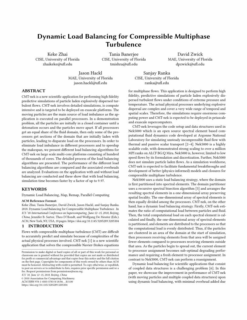
Figure 11 shows a comparison between the adaptive load-balancing

and user-triggered load-balancing algorithms. For the user-triggered

load-balancing algorithm, the k = 500, thus load balance is trig-

gered every 500 time steps. As we can see from the figure, there is

no performance degradation in the first 4, 000 time steps, making

any load balancing redundant during this time. However, right after

step 4, 000 performance degrades sharply, requiring frequent load-

balancing. The user-triggered load-balancing algorithm is insensi-

tive to these performance variations and continues to load balance

every 500 time steps. The average time per time step from step


0

1

2

3

4

5

6

7

8

9

10

0 1000 2000 3000 4000 5000 6000

Tim

e p

er

Tim

e S

tep (

seco

nds)


AdaptiveLB UserTriggeredLB

Figure 11: Performance comparison between adaptive load-balanced and user-triggered load balanced versions of CMT-nek on Vulcan. They were run on 32, 768 MPI ranks, thatis 8, 192 nodes with 4 cores per node. Distributed load-balancing algorithmwas used. The timeper time step for theuser-triggered and the adaptive load-balanced versions was4.17 and 3.78 seconds, respectively, for the last 2, 000 steps,giving us an overall improvement of 9.4%.4, 000 to step 6, 000 taken by the adaptive and user-triggered load-

balancing versions was 3.78 and 4.17 seconds, respectively. Thus,

adaptive load-balancing algorithm gained an overall improvement

of 9.4% compared to the user specified triggered load-balancing

algorithm, and further the load balancing happens automatically

without requiring any intervention by the user.

6 CONCLUSIONIn this paper, we have shown that an architecture-independent

mapping that reorders the spectral elements (and corresponding

particles), followed by mapping and remapping the ordered spec-

tral elements is an effective strategy for load balancing CMT-nek, a

compressible, multiphase turbulent flow application. We have devel-

oped centralized, distributed and hybrid load-balancing algorithms

and have studied their comparative overheads on two platforms,

namely, Intel Broadwell and IBM BG/Q. Our results show that using

this approach, we can potentially scale the application up to several

million cores and still achieve reasonable load-balancing overhead

and overall load balance. Using our load-balanced code we obtained

a speed-up factor of up to 9.97. Given that scientific applications

run simulations for weeks, this speed-up is significant since it will

not only save valuable computing resources, but due to smaller

execution times, will also result in fewer runtime failures. We also

presented a simple adaptive load-balancing strategy which automat-

ically triggers load balancing when needed. Compared to the user

triggered load balancing, the adaptive load balancing strategy can

additionally save time up to 9.4%. The current work was focused

on one-dimensional expansion of particles. For many simulations,

this expansion happens in two (cylindrical) or three (spherical) di-

mensions. We believe that improvements using our load-balancing

schemes will be even larger than for the one-dimensional expansion

reported in this paper.

ACKNOWLEDGMENTThis work was funded by the U.S. Department of Energy, National

Nuclear Security Administration, Advanced Simulation and Com-

puting Program, as a Cooperative Agreement under the Predictive

Science Academic Alliance Program, Contract No. DOE-NA0002378.

This material is based upon work supported by the National Science

Foundation Graduate Research Fellowship under Grant No. DGE-

1315138.

REFERENCES[1] T. Banerjee, J. Hackl, M. Shringarpure, T. Islam, S. Balachandar, T. Jackson, and

S. Ranka. Cmt-bone—a proxy application for compressible multiphase turbulent

flows. In High Performance Computing (HiPC), 2016 IEEE 23rd InternationalConference on, pages 173–182. IEEE, 2016.

[2] H.M. Tufo and P.F. Fischer. Terascale spectral element algorithms and implemen-

tations. In In Proceedings of the 1999 ACM/IEEE conference on Supercomputing,page 68. ACM, 1999.

[3] P. F. Fischer, J. Lottes, S. Kerkemeier, K. Heisey, A. Obabko, O. Marin, and

E. Merzari. http://nek5000.mcs.anl.gov, 2014.

[4] M. Deville, P. Fischer, and E. Mund. High-order methods for incompressible fluidflow, volume 9. Cambridge University Press, 2002.

[5] B. Hendrickson and R. Leland. Multidimensional spectral load balancing. Tech-

nical report, Sandia National Labs., Albuquerque, NM (United States), 1993.

[6] A. Choudhary, G. Fox, S. Hiranandani, K. Kennedy, C. Koelbel, S. Ranka, and

J. Saltz. Software support for irregular and loosely synchronous problems. Com-puting Systems in Engineering, 3(1-4):43–52, 1992.

[7] M. Lieber and W. Nagel. Highly scalable sfc-based dynamic load balancing and

its application to atmospheric modeling. Future Generation Computer Systems,2017.

[8] H. Menon, N. Jain, G. Zheng, and L. Kale. Automated load balancing invocation

based on application characteristics. In Cluster Computing (CLUSTER), 2012 IEEEInternational Conference on, pages 373–381. IEEE, 2012.

[9] I. Surmin, A. Bashinov, S. Bastrakov, E. Efimenko, A. Gonoskov, and I. Meyerov.

Dynamic load balancing based on rectilinear partitioning in particle-in-cell

plasma simulation. In International Conference on Parallel Computing Technologies,pages 107–119. Springer, 2015.

[10] R. Ferraro, P. Liewer, and V. Decyk. Dynamic load balancing for a 2d concurrent

plasma pic code. Journal of computational physics, 109(2):329–341, 1993.[11] S. Plimpton, D. Seidel, M. Pasik, R. Coats, and G. Montry. A load-balancing

algorithm for a parallel electromagnetic particle-in-cell code. Computer physicscommunications, 152(3):227–241, 2003.

[12] K. Germaschewski, W. Fox, S. Abbott, N. Ahmadi, K. Maynard, L. Wang, H. Ruhl,

and A. Bhattacharjee. The plasma simulation code: A modern particle-in-cell

code with load-balancing and gpu support. arXiv preprint arXiv:1310.7866, 2013.[13] H. Nakashima, Y. Miyake, H. Usui, and Y. Omura. Ohhelp: a scalable domain-

decomposing dynamic load balancing for particle-in-cell simulations. In Proceed-ings of the 23rd international conference on Supercomputing, pages 90–99. ACM,

2009.

[14] O. Pearce, T. Gamblin, B. De Supinski, T. Arsenlis, and N. Amato. Load balancing

n-body simulations with highly non-uniform density. In Proceedings of the 28thACM international conference on Supercomputing, pages 113–122. ACM, 2014.

[15] A. Bhatelé, L. Kalé, and S. Kumar. Dynamic topology aware load balancing

algorithms for molecular dynamics applications. In Proceedings of the 23rdinternational conference on Supercomputing, pages 110–116. ACM, 2009.

[16] I. Al-Furajh, S. Aluru, S. Goil, and S. Ranka. Parallel construction of multidimen-

sional binary search trees. IEEE Transactions on Parallel and Distributed Systems,11(2):136–148, 2000.

[17] S. Ranka, R. Shankar, and K. Alsabti. Many-to-many personalized communica-

tion with bounded traffic. In Frontiers of Massively Parallel Computation, 1995.Proceedings. Frontiers’ 95., Fifth Symposium on the, pages 20–27. IEEE, 1995.

[18] J. Hackl, M. Shringarpure, R. Koneru, M. Delchini, and S. Balachandar. A shock

capturing discontinuous Galerkin spectral element method for curved geometry

using entropy viscosity. Computers and Fluids.[19] S. Gottlieb and C.-W. Shu. Total variation-diminishing Runge-Kutta schemes.

Math. Comp., 67:73–85, 1998.[20] J. P. Berrut and L. N. Trefethen. Barycentric lagrange interpolation. SIAM review,

46(3):501–517, 2004.

[21] C. W. Ou and S. Ranka. Parallel remapping of adaptive problems. J. ParallelDistrib. Comput., 42(2):109–121, May 1997.

[22] C. W. Ou, S. Ranka, and G. Fox. Fast and parallel mapping algorithms for irregular

problems. The Journal of Supercomputing, 10(2):119–140, Jun 1996.

[23] C. W. Ou, M. Gunwani, and S. Ranka. Architecture-independent locality-

improving transformations of computational graphs embedded in k-dimensions.

In Proceedings of the 9th International Conference on Supercomputing, ICS ’95,

pages 289–298, New York, NY, USA, 1995. ACM.

[24] H. M. Tufo and P. F. Fischer. Fast parallel direct solvers for coarse grid problems.

J. Parallel Distrib. Comput., 61(2):151–177, February 2001.

[25] T. Banerjee and S. Ranka. A genetic algorithm based autotuning approach for

performance and energy optimization. In Green Computing Conference andSustainable Computing Conference (IGSC), 2015 Sixth International, pages 1–8.IEEE, 2015.

Documents

Dynamic Load Balancing for Compressible Multiphase Turbulenceics2018.ict.ac.cn/essay/ics18-final62.pdf · Dynamic load balancing for scientific applications that consist of coupled