Dynamic Information and Constraints in Source and Channel

Dynamic Information and Constraints

in Source and Channel Coding

by

Emin Martinian

B.S., University of California at Berkeley (1997)S.M., Massachusetts Institute of Technology (2000)

Submitted to the Department of Electrical Engineering and Computer Sciencein partial fulfillment of the requirements for the degree of

Doctor of Philosophy in Electrical Engineering and Computer Science

at the

MASSACHUSETTS INSTITUTE OF TECHNOLOGY

September 2004

c© Massachusetts Institute of Technology 2004. All rights reserved.

Author . . . . . . . . . . . . . . . . . . . . . . . . . . . . . . . . . . . . . . . . . . . . . . . . . . . . . . . . . . . . . . . . . . . . . . . . . . . .Department of Electrical Engineering and Computer Science

September 1, 2004

Certified by. . . . . . . . . . . . . . . . . . . . . . . . . . . . . . . . . . . . . . . . . . . . . . . . . . . . . . . . . . . . . . . . . . . . . . . .Gregory W. Wornell

Professor of Electrical Engineering and Computer ScienceThesis Supervisor

Accepted by . . . . . . . . . . . . . . . . . . . . . . . . . . . . . . . . . . . . . . . . . . . . . . . . . . . . . . . . . . . . . . . . . . . . . . .Arthur C. Smith

Chairman, Department Committee on Graduate Students

2

Abstract

This thesis explore dynamics in source coding and channel coding.We begin by introducing the idea of distortion side information, which does not di-

rectly depend on the source but instead affects the distortion measure. Such distortion

side information is not only useful at the encoder but under certain conditions knowing itat the encoder is optimal and knowing it at the decoder is useless. Thus distortion side

information is a natural complement to Wyner-Ziv side information and may be useful inexploiting properties of the human perceptual system as well as in sensor or control applica-tions. In addition to developing the theoretical limits of source coding with distortion side

information, we also construct practical quantizers based on lattices and codes on graphs.Our use of codes on graphs is also of independent interest since it highlights some issues in

translating the success of turbo and LDPC codes into the realm of source coding.Finally, to explore the dynamics of side information correlated with the source, we

consider fixed lag side information at the decoder. We focus on the special case of perfect

side information with unit lag corresponding to source coding with feedforward (the dualof channel coding with feedback). Using duality, we develop a linear complexity algorithm

which exploits the feedforward information to achieve the rate-distortion bound.The second part of the thesis focuses on channel dynamics in communication by intro-

ducing a new system model to study delay in streaming applications. We first consider an

adversarial channel model where at any time the channel may suffer a burst of degradedperformance (e.g., due to signal fading, interference, or congestion) and prove a coding

theorem for the minimum decoding delay required to recover from such a burst. Our cod-ing theorem illustrates the relationship between the structure of a code, the dynamics ofthe channel, and the resulting decoding delay. We also consider more general channel dy-

namics. Specifically, we prove a coding theorem establishing that, for certain collections ofchannel ensembles, delay-universal codes exist that simultaneously achieve the best delay

for any channel in the collection. Practical constructions with low encoding and decodingcomplexity are described for both cases.

Finally, we also consider architectures consisting of both source and channel coding

which deal with channel dynamics by spreading information over space, frequency, multipleantennas, or alternate transmission paths in a network to avoid coding delays. Specifically,

we explore whether the inherent diversity in such parallel channels should be exploited atthe application layer via multiple description source coding, at the physical layer via paral-lel channel coding, or through some combination of joint source-channel coding. For on-off

channel models application layer diversity architectures achieve better performance whilefor channels with a continuous range of reception quality (e.g., additive Gaussian noise

channels with Rayleigh fading), the reverse is true. Joint source-channel coding achievesthe best of both by performing as well as application layer diversity for on-off channels and

as well as physical layer diversity for continuous channels.

Supervisor: Gregory W. WornellTitle: Professor of Electrical Engineering and Computer Science

3

4

Acknowledgments

Completing this thesis reminds how much I have learned from my friends, family, andcolleagues and the debt of gratitude I owe them.

The most important reason for my success at MIT is my advisor, Gregory Wornell. He

taught me how to think about research, how to see the big picture without being distractedby technical details, and how not to give up until such details are resolved. I am alsodeeply grateful for Greg’s wisdom, patience, and friendship. Graduate school contains

periods where every idea seems to fail and it is easy to become discouraged. Greg providedencouragement during these times while also explaining how they are essential in learning

to think independently.

I would also like to thank Greg and Prof. Alan Oppenheim for bringing together such awonderful collection of people in the Signals, Information, and Algorithms Laboratory and

the Digital Signal Processing Group. I learned a lot from everyone in the group especiallyRichard Barron, Albert Chan, Brian Chen, Aaron Cohen, Vijay Divi, Stark Draper, YoninaEldar, Uri Erez, Everest Huang, Ashish Khisti, Nicholas Laneman, Mike Lopez, Andrew

Russel, Maya Said, Charles Sestok, Charles Swannack, Huan Yao, and Ram Zamir. Nickand Stark in particular were mentors to me and I fondly remember the many conversations,

basketball games, and conferences we enjoyed together. Finally, no student scrambling tosubmit a paper or finish a thesis can fail to appreciate the value of an excellent systemadministrator and administrative assistant like Giovanni Aliberti and Tricia Mulcahy.

The members of my thesis committee, Prof. Dave Forney, Prof. Ram Zamir, and Prof.Lizhong Zheng deserve special thanks for their efforts in reading the thesis and offeringtheir advice. During his sabbatical at MIT, Prof. Zamir introduced me to high resolution

rate-distortion theory and inspired many of the ideas in Chapters 2 and 3. Also, Prof.Forney’s comments on Chapter 4 and Prof. Zheng’s remarks about possible applications of

the ideas in Chapter 3 to channel coding were especially helpful.

Various internships were an important complement to my time at MIT. Working withCarl-Erik Sundberg at Lucent Technologies’ Bell Labs was valuable in understanding re-search problems from an industrial perspective. Working at Bell Labs sparked my interest

in low delay coding and led to Chapters 6–9. While at Bell Labs, I also had the pleasure tomeet Ramesh Johari who has been a lunch companion and friend ever since. I am grateful

to Ramesh for reminding me how much I enjoyed MIT on the (few) occasions I complainedabout graduate school and for many other interesting observations.

Visits to Hewlett-Packard Labs sponsored by the HP-MIT Alliance were also a stimu-

lating and memorable experience. In particular, an argument between Nick, John Apos-tolopoulos, Susie Wee, and I during one such visit led to the research described in Chap-ter 10. Mitch Trott’s wry advice, culinary knowledge, and thoughts about research were

another highlight of visiting HP and Chapter 8 is one result of our collaboration.

Jonathan Yedidia hired me for a wonderful summer at Mitsubishi Electronic ResearchLabs and helped me see electrical engineering from a fresh perspective. I am especially

grateful to Jonathan for teaching me about belief propagation and taking a chance on mystrange idea about source coding with codes on graphs described in Chapter 4.

Finally, I would like to thank my family and friends. My parents, my aunt and uncle,

Monica and Reuben Toumani, and my second family, the Malkins, provided much appreci-ated love, encouragement and support. Alex Aravanis, Jarrod Chapman, and Mike Malkin

have my gratitude for their warm friendship and good company. The conversations we hadabout science, math and engineering over the years are what inspired me to pursue graduate

5

studies in engineering instead of seeking my fortune in another career. In Boston I wouldlike to thank Orissa, Putney, and Adelle Lawrence, and Joyce Baker for helping me adjust

to life here.Most of all I would like to thank my wife Esme. Her love, sense of humor, and friendship

have made these past six years in Boston the best time of my life. If not for her, I would

never have come to MIT and never completed this thesis.

This research was supported by the National Science Foundation through grants and a

National Science Foundation Graduate Fellowship and by the HP-MIT Alliance.

6

To my parents Medea and Omega,and their efforts for my education

7

Bibliographic Note

Portions of Chapter 2 were presented at the Data Compression Conference [124] and theInternational Symposium on Information Theory [123] with co-authors Gregory W. Wornell

and Ram Zamir.

Chapter 4 is joint work with Jonathan S. Yedidia and was presented at the Allerton

conference [125].

Chapter 5 is joint work with Gregory W. Wornell and will be presented at the forty-second annual Allerton conference in Monticello, IL in October 2004.

Portions of Chapter 9 were presented at the Allerton conference [122] with co-authorGregory W. Wornell.

Chapter 10 is joint work with J. Nicholas Laneman, Gregory W. Wornell, and John G.

Apostolopoulos and has been submitted to the Transactions on Information Theory as wellas presented in part (with Susie Wee as additional co-author) at the International Conferenceon Communications [96] and the International Symposium on Information Theory [95].

8

Contents

1 Introduction 19

1.1 Distributed Information in Source Coding . . . . . . . . . . . . . . . . . . . 20

1.1.1 Distortion Side Information . . . . . . . . . . . . . . . . . . . . . . . 20

1.1.2 Fixed Lag Signal Side Information . . . . . . . . . . . . . . . . . . . 21

1.2 Delay Constraints . . . . . . . . . . . . . . . . . . . . . . . . . . . . . . . . . 21

1.2.1 Streaming Codes For Bursty Channels . . . . . . . . . . . . . . . . . 22

1.2.2 Delay Universal Streaming Codes . . . . . . . . . . . . . . . . . . . . 23

1.2.3 Low Delay Application and Physical Layer Diversity Architectures . 26

1.3 Outline of the Thesis . . . . . . . . . . . . . . . . . . . . . . . . . . . . . . . 27

I Distributed Information In Source Coding 28

2 Distortion Side Information 29

2.1 Introduction . . . . . . . . . . . . . . . . . . . . . . . . . . . . . . . . . . . . 30

2.2 Examples . . . . . . . . . . . . . . . . . . . . . . . . . . . . . . . . . . . . . 31

2.2.1 Discrete Uniform Source . . . . . . . . . . . . . . . . . . . . . . . . . 31

2.2.2 Gaussian Source . . . . . . . . . . . . . . . . . . . . . . . . . . . . . 32

2.3 Problem Model . . . . . . . . . . . . . . . . . . . . . . . . . . . . . . . . . . 33

2.4 Finite Resolution Quantization . . . . . . . . . . . . . . . . . . . . . . . . . 34

2.4.1 Uniform Sources with Group Difference Distortions . . . . . . . . . . 36

2.4.2 Examples . . . . . . . . . . . . . . . . . . . . . . . . . . . . . . . . . 37

2.4.3 Erasure Distortions . . . . . . . . . . . . . . . . . . . . . . . . . . . . 40

2.5 Asymptotically High-Resolution Quantization . . . . . . . . . . . . . . . . . 41

2.5.1 Technical Conditions . . . . . . . . . . . . . . . . . . . . . . . . . . . 41

2.5.2 Equivalence Theorems . . . . . . . . . . . . . . . . . . . . . . . . . . 42

2.5.3 Penalty Theorems . . . . . . . . . . . . . . . . . . . . . . . . . . . . 44

2.6 Finite Rate Bounds For Quadratic Distortions . . . . . . . . . . . . . . . . . 45

2.6.1 A Medium Resolution Bound . . . . . . . . . . . . . . . . . . . . . . 46

2.6.2 A Low Resolution Bound . . . . . . . . . . . . . . . . . . . . . . . . 46

2.6.3 A Finite Rate Gaussian Example . . . . . . . . . . . . . . . . . . . . 47

2.7 Discussion . . . . . . . . . . . . . . . . . . . . . . . . . . . . . . . . . . . . . 48

2.7.1 Applications to Sensors and Sensor Networks . . . . . . . . . . . . . 48

2.7.2 Richer Distortion Models and Perceptual Coding . . . . . . . . . . . 50

2.7.3 Decomposing Side Information Into q and w . . . . . . . . . . . . . 51

2.8 Concluding Remarks . . . . . . . . . . . . . . . . . . . . . . . . . . . . . . . 52

9

2.8.1 Possibilities For Future Work . . . . . . . . . . . . . . . . . . . . . . 52

3 Low Complexity Quantizers For Distortion Side Information 53

3.1 Introduction . . . . . . . . . . . . . . . . . . . . . . . . . . . . . . . . . . . . 54

3.2 Two Simple Examples . . . . . . . . . . . . . . . . . . . . . . . . . . . . . . 56

3.2.1 Discrete Uniform Source . . . . . . . . . . . . . . . . . . . . . . . . . 56

3.2.2 Weighted Quadratic Distortion . . . . . . . . . . . . . . . . . . . . . 57

3.3 Notation . . . . . . . . . . . . . . . . . . . . . . . . . . . . . . . . . . . . . . 60

3.4 Lattice Quantizer Structures . . . . . . . . . . . . . . . . . . . . . . . . . . 60

3.4.1 A Brief Review of Lattices and Cosets . . . . . . . . . . . . . . . . . 62

3.4.2 The Fully Informed System . . . . . . . . . . . . . . . . . . . . . . . 63

3.4.3 The Partially Informed System . . . . . . . . . . . . . . . . . . . . . 63

3.5 Efficient Encoding and Performance . . . . . . . . . . . . . . . . . . . . . . 66

3.5.1 The Encoding Algorithm . . . . . . . . . . . . . . . . . . . . . . . . 66

3.5.2 An Example of Encoding . . . . . . . . . . . . . . . . . . . . . . . . 67

3.5.3 Complexity Analysis . . . . . . . . . . . . . . . . . . . . . . . . . . . 68

3.5.4 Statistical Models and Distortion Measures . . . . . . . . . . . . . . 68

3.5.5 Rate-Distortion For Fully Informed Systems . . . . . . . . . . . . . . 69

3.5.6 Rate-Distortion For Partially Informed Systems . . . . . . . . . . . . 71


4 Iterative Quantization Using Codes On Graphs 73

4.1 Introduction . . . . . . . . . . . . . . . . . . . . . . . . . . . . . . . . . . . . 74

4.2 Quantization Model . . . . . . . . . . . . . . . . . . . . . . . . . . . . . . . 74

4.2.1 Binary Erasure Quantization . . . . . . . . . . . . . . . . . . . . . . 75

4.3 Codes For Erasure Quantization . . . . . . . . . . . . . . . . . . . . . . . . 75

4.3.1 LDPC Codes Are Bad Quantizers . . . . . . . . . . . . . . . . . . . 76

4.3.2 Dual LDPC Codes . . . . . . . . . . . . . . . . . . . . . . . . . . . . 77

4.3.3 Optimal Quantization/Decoding and Duality . . . . . . . . . . . . . 77

4.3.4 Iterative Decoding/Quantization and Duality . . . . . . . . . . . . . 78


5 Source Coding with Fixed Lag Side Information 83

5.1 Introduction . . . . . . . . . . . . . . . . . . . . . . . . . . . . . . . . . . . . 84

5.2 Problem Description . . . . . . . . . . . . . . . . . . . . . . . . . . . . . . . 85

5.3 Example: Binary Source & Erasure Distortion . . . . . . . . . . . . . . . . . 86

5.4 Example: Binary Source & Hamming Distortion . . . . . . . . . . . . . . . 87

5.5 Finite Alphabet Sources & Arbitrary Distortion . . . . . . . . . . . . . . . . 89

5.5.1 Feedforward Source Coding Subsystems . . . . . . . . . . . . . . . . 89

5.5.2 Feedforward Encoder and Decoder . . . . . . . . . . . . . . . . . . . 90

5.5.3 Rate-Distortion Analysis . . . . . . . . . . . . . . . . . . . . . . . . . 91


II Delay Constraints 93

6 System Model 95

6.0.1 Notation . . . . . . . . . . . . . . . . . . . . . . . . . . . . . . . . . . 96

10

6.1 Channel Models . . . . . . . . . . . . . . . . . . . . . . . . . . . . . . . . . . 96

6.2 Notions Of Delay . . . . . . . . . . . . . . . . . . . . . . . . . . . . . . . . . 97

6.2.1 Block-Delay . . . . . . . . . . . . . . . . . . . . . . . . . . . . . . . . 97

6.2.2 Symbol-Delay . . . . . . . . . . . . . . . . . . . . . . . . . . . . . . . 98

6.2.3 Packet-Delay . . . . . . . . . . . . . . . . . . . . . . . . . . . . . . . 98

7 Streaming Codes For Bursty Channels 101

7.1 A Gaussian Example . . . . . . . . . . . . . . . . . . . . . . . . . . . . . . . 102

7.2 Problem Model . . . . . . . . . . . . . . . . . . . . . . . . . . . . . . . . . . 103

7.2.1 Defining Burst-Delay Capacity . . . . . . . . . . . . . . . . . . . . . 105

7.3 Computing Burst-Delay Capacity . . . . . . . . . . . . . . . . . . . . . . . . 106

7.4 The Converse of the Burst-Delay Capacity Theorem . . . . . . . . . . . . . 107

7.5 The Direct Part of the Burst-Delay Capacity Theorem . . . . . . . . . . . . 108

7.5.1 Coding Scheme Overview . . . . . . . . . . . . . . . . . . . . . . . . 109

7.5.2 Encoding . . . . . . . . . . . . . . . . . . . . . . . . . . . . . . . . . 109

7.5.3 Decoding . . . . . . . . . . . . . . . . . . . . . . . . . . . . . . . . . 113

7.6 Single Path Examples . . . . . . . . . . . . . . . . . . . . . . . . . . . . . . 116

7.6.1 An Erasure Channel Example . . . . . . . . . . . . . . . . . . . . . . 116

7.6.2 A Single Path Binary Symmetric Channel Example . . . . . . . . . . 117

7.7 Practical Coding Schemes . . . . . . . . . . . . . . . . . . . . . . . . . . . . 119


8 Delay-Optimal Burst Erasure Code Constructions 121

8.1 Problem Model . . . . . . . . . . . . . . . . . . . . . . . . . . . . . . . . . . 122

8.2 Single-Link Codes . . . . . . . . . . . . . . . . . . . . . . . . . . . . . . . . 122

8.2.1 Reed-Solomon Codes Are Not Generally Optimal . . . . . . . . . . . 125

8.2.2 Provably Optimal Construction For All Rates . . . . . . . . . . . . . 125

8.3 Two-Link Codes . . . . . . . . . . . . . . . . . . . . . . . . . . . . . . . . . 129

8.3.1 Constructions . . . . . . . . . . . . . . . . . . . . . . . . . . . . . . . 129

8.4 Multi-Link Codes . . . . . . . . . . . . . . . . . . . . . . . . . . . . . . . . . 133

8.5 Codes For Stochastically Any Degraded Channel . . . . . . . . . . . . . . . 134


9 Delay Universal Streaming Codes 137

9.1 Previous Work . . . . . . . . . . . . . . . . . . . . . . . . . . . . . . . . . . 139

9.2 Stream Coding System Model . . . . . . . . . . . . . . . . . . . . . . . . . . 140

9.2.1 The Achievable Delay Region . . . . . . . . . . . . . . . . . . . . . . 141

9.3 Coding Theorems . . . . . . . . . . . . . . . . . . . . . . . . . . . . . . . . . 143

9.3.1 Information Debt . . . . . . . . . . . . . . . . . . . . . . . . . . . . . 144

9.3.2 Random Code Constructions . . . . . . . . . . . . . . . . . . . . . . 145

9.4 Code Constructions . . . . . . . . . . . . . . . . . . . . . . . . . . . . . . . 146

9.5 Delay and Stability Analysis . . . . . . . . . . . . . . . . . . . . . . . . . . . 151

9.5.1 An Erasure Channel Example . . . . . . . . . . . . . . . . . . . . . . 152


11

10 Low Delay Application and Physical Layer Diversity Architectures 157

10.1 Introduction . . . . . . . . . . . . . . . . . . . . . . . . . . . . . . . . . . . . 158

10.1.1 Related Research . . . . . . . . . . . . . . . . . . . . . . . . . . . . . 161

10.1.2 Outline . . . . . . . . . . . . . . . . . . . . . . . . . . . . . . . . . . 162

10.2 System Model . . . . . . . . . . . . . . . . . . . . . . . . . . . . . . . . . . . 162

10.2.1 Notation . . . . . . . . . . . . . . . . . . . . . . . . . . . . . . . . . . 162

10.2.2 Source Model . . . . . . . . . . . . . . . . . . . . . . . . . . . . . . . 163

10.2.3 (Parallel) Channel Model . . . . . . . . . . . . . . . . . . . . . . . . 163

10.2.4 Architectural Options . . . . . . . . . . . . . . . . . . . . . . . . . . 164

10.2.5 High-Resolution Approximations for Source Coding . . . . . . . . . 167

10.3 On-Off Component Channels . . . . . . . . . . . . . . . . . . . . . . . . . . 169

10.3.1 Component Channel Model . . . . . . . . . . . . . . . . . . . . . . . 169

10.3.2 No Diversity . . . . . . . . . . . . . . . . . . . . . . . . . . . . . . . 170

10.3.3 Optimal Channel Coding Diversity . . . . . . . . . . . . . . . . . . . 170

10.3.4 Source Coding Diversity . . . . . . . . . . . . . . . . . . . . . . . . . 172

10.3.5 Comparison . . . . . . . . . . . . . . . . . . . . . . . . . . . . . . . . 173

10.4 Continuous State Channels . . . . . . . . . . . . . . . . . . . . . . . . . . . 175

10.4.1 Continuous Channel Model . . . . . . . . . . . . . . . . . . . . . . . 175

10.4.2 No Diversity . . . . . . . . . . . . . . . . . . . . . . . . . . . . . . . 176

10.4.3 Selection Channel Coding Diversity . . . . . . . . . . . . . . . . . . 177

10.4.4 Multiplexed Channel Coding Diversity . . . . . . . . . . . . . . . . . 178

10.4.5 Optimal Channel Coding Diversity . . . . . . . . . . . . . . . . . . . 179

10.4.6 Source Coding Diversity . . . . . . . . . . . . . . . . . . . . . . . . . 179

10.4.7 Rayleigh Fading AWGN Example . . . . . . . . . . . . . . . . . . . . 180

10.5 Source Coding Diversity with Joint Decoding . . . . . . . . . . . . . . . . . 183

10.5.1 System Description . . . . . . . . . . . . . . . . . . . . . . . . . . . . 183

10.5.2 Performance . . . . . . . . . . . . . . . . . . . . . . . . . . . . . . . 185


11 Concluding Remarks 189

11.1 Distortion Side Information Models . . . . . . . . . . . . . . . . . . . . . . . 190

11.2 Delay . . . . . . . . . . . . . . . . . . . . . . . . . . . . . . . . . . . . . . . 191

A Notation Summary 193

B Distortion Side Information Proofs 195

B.1 Group Difference Distortion Measures Proof . . . . . . . . . . . . . . . . . . 196

B.2 Binary-Hamming Rate-Distortion Derivations . . . . . . . . . . . . . . . . . 196

B.2.1 With Encoder Side Information . . . . . . . . . . . . . . . . . . . . . 196

B.2.2 Without Encoder Side Information . . . . . . . . . . . . . . . . . . . 197

B.3 High-Resolution Proofs . . . . . . . . . . . . . . . . . . . . . . . . . . . . . . 198

B.4 Finite Resolution Bounds . . . . . . . . . . . . . . . . . . . . . . . . . . . . 204

C Iterative Quantization Proofs 209

D Information/Operational R(D) Equivalence 213

E Proofs For Burst-Delay Codes 215

12

F Proofs for Burst Correcting Code Constructions 217

G Proofs For Delay Universal Streaming Codes 221

H Distortion Exponent Derivations 227H.1 Distortion Exponent For Selection Channel Coding Diversity . . . . . . . . 228H.2 Distortion Exponent For Multiplexed Channel Coding Diversity . . . . . . . 228

H.3 Distortion Exponent for Optimal Channel Coding Diversity . . . . . . . . . 229H.4 Distortion Exponent for Source Coding Diversity . . . . . . . . . . . . . . . 231

H.5 Distortion Exponent for Source Coding Diversity with Joint Decoding . . . 232

13

14

List of Figures

1-1 Source coding with fixed lag side information. . . . . . . . . . . . . . . . . . 21

1-2 Optimal code for correcting bursts of λs lost packets with delay λ(ms + 1). 24

1-3 Channels with same number of erasures but different dynamics. . . . . . . 25

1-4 Diagrams for (a) channel coding diversity and (b) source coding diversity. . 27

2-1 Example of binary distortion side information. . . . . . . . . . . . . . . . . 32

2-2 Scenarios for source coding with side information. . . . . . . . . . . . . . . . 34

2-3 Quantizers for distortion side information known at encoder and decoder. . 35

2-4 Quantizers for distortion side information known only at then encoder. . . . 36

2-5 First binary source, Hamming distortion example. . . . . . . . . . . . . . . 39

2-6 Second binary source, Hamming distortion example. . . . . . . . . . . . . . 40

2-7 Distortion side information results for continuous sources. . . . . . . . . . . 42

2-8 Gaussian-Quadratic distortion side information example. . . . . . . . . . . . 49

3-1 Example of binary distortion side information. . . . . . . . . . . . . . . . . 56

3-2 Lattice quantizers for distortion side information at encoder and decoder. . 58

3-3 Variable codebook and partition view of the quantizers in Fig. 3-2. . . . . . 59

3-4 Lattice quantizers for distortion side information known only at encoder. . . 60

3-5 A fixed codebook/variable partition view of the quantizers in Fig. 3-4. . . . 61

4-1 Using an LDPC code for binary erasure quantization. . . . . . . . . . . . . 76

4-2 Using the dual of an LDPC code for binary erasure quantization. . . . . . . 77

5-1 Source coding with fixed lag side information. . . . . . . . . . . . . . . . . . 84

5-2 Encoder and decoder for an erasure channel with feedback. . . . . . . . . . 86

5-3 Encoder and decoder for an erasure source with feedforward. . . . . . . . . 87

6-1 Illustration of a system with a bit-delay of 20. . . . . . . . . . . . . . . . . 98

7-1 The low delay burst correction problem model. . . . . . . . . . . . . . . . . 104

7-2 Illustration of burst sequence used in proof of Theorem 22. . . . . . . . . . 108

8-1 General form for a linear, feedback-free, rate k/n, memory M packet encoder. 123

8-2 A convolutional code structure based on diagonal interleaving. . . . . . . . 124

8-3 Delay-optimal erasure burst correcting block code structure. . . . . . . . . . 126

8-4 A channel with two transmission links. . . . . . . . . . . . . . . . . . . . . 129

8-5 Two-link, delay-optimal, erasure burst correcting block code structure. . . . 131

15

9-1 Channels with same number of erasures but different dynamics. . . . . . . 1389-2 Conceptual illustration of possible delay region. . . . . . . . . . . . . . . . . 142

9-3 Bounds on decoding delay for an erasure channel. . . . . . . . . . . . . . . . 1539-4 Bounds on decoding delay distribution for a memoryless packet loss channel. 154

10-1 The parallel diversity coding problem. . . . . . . . . . . . . . . . . . . . . . 15810-2 Diagrams for (a) channel coding diversity and (b) source coding diversity. . 15910-3 Decoding regions for source and channel diversity systems. . . . . . . . . . . 160

10-4 Channel coding diversity. . . . . . . . . . . . . . . . . . . . . . . . . . . . . 16510-5 Source coding diversity system model. . . . . . . . . . . . . . . . . . . . . . 166

10-6 Source coding diversity with joint source-channel decoding. . . . . . . . . . 16710-7 Outage regions for optimal parallel channel coding. . . . . . . . . . . . . . . 17110-8 Average distortion performance for terms in (10.37). . . . . . . . . . . . . . 172

10-9 Outage region boundaries for MD source coding. . . . . . . . . . . . . . . . 17310-10Average distortion performance over on-off channels. . . . . . . . . . . . . . 174

10-11Distortion exponents versus bandwidth expansion factor. . . . . . . . . . . . 18210-12Average distortion on a Rayleigh fading channel. . . . . . . . . . . . . . . . 18210-13Conceptual diagram of an MD quantizer. . . . . . . . . . . . . . . . . . . . 183

10-14Decoding regions for a joint source-channel decoder. . . . . . . . . . . . . . 184

F-1 How a burst affects the constituent interleaved block codes. . . . . . . . . . 218

16

List of Tables

2.1 Asymptotic rate-penalty in nats. Euler’s constant is denoted by γ. . . . . . 45

4.1 An algorithm for iteratively decoding data with erasures. . . . . . . . . . . 79

4.2 An algorithm for iteratively quantizing a source with erasures. . . . . . . . 80

5.1 The Feedforward Encoder. . . . . . . . . . . . . . . . . . . . . . . . . . . . 90

5.2 The Feedforward Decoder. . . . . . . . . . . . . . . . . . . . . . . . . . . . 90

7.1 Illustration of how a source packet is divided into M · L pieces. . . . . . . . . 110

7.2 Description of how s [i]’s are interleaved to produce v[i, p]’s. . . . . . . . . 1117.3 Encoding example for a rate R = 3/5 single path code. . . . . . . . . . . . . 1177.4 Encoding example for a burst binary symmetric channel. . . . . . . . . . . . 118

8.1 A rate 3/5 convolutinal code constructed via diagonal interleaving. . . . . . 1258.2 Construction of a two-link block code via diagonal interleaving. . . . . . . . 130

9.1 The algorithm VANDERMONDE-ELIMINATE(C). . . . . . . . . . . 148

10.1 Source coding diversity decoder rules. . . . . . . . . . . . . . . . . . . . . . 166

10.2 Distortion exponents. . . . . . . . . . . . . . . . . . . . . . . . . . . . . . . . 181

G.1 Relationship between channel sequences used in proof of Lemma 7. . . . . . 222

17

18

Chapter 1

Introduction

19

Communication channels, data sources, and distortion measures that vary during com-pression or communication of the data stream are the focus of this thesis. Specifically,

our goal is to understand how such model dynamics affect the fundamental limits of com-munication and compression and to understand how to design efficient systems. The keydifferences between static and dynamic scenarios are knowledge and delay: learning the

system state and averaging over a long enough period essentially makes these two scenariosequivalent. Thus our main questions can be summarized as “What are the effects of dis-

tributed, imperfect, or missing knowledge of state information?” and “What are the effectsof delay constraints?”. After outlining our approach to these questions in the rest of thischapter, we explore the former mostly in the context of source coding in Part I and the

latter mostly in the context of channel coding in Part II.

� 1.1 Distributed Information in Source Coding

� 1.1.1 Distortion Side Information

In the classical source coding problem, an encoder is given a source signal, s, and must

represent it using R bits per sample. Performance is measured by a distortion function,d(s, s), which describes the cost of quantizing a source sample with the value s to s. In

many applications, however, the appropriate distortion function depends on a notion ofquality which varies dynamically and no static distortion model is appropriate.

For example, a sensor may obtain measurements of a signal along with some estimate ofthe quality of such measurements. This may occur if the sensor can calibrate its accuracyto changing conditions (e.g., the amount of light, background noise, or other interference

present), if the sensor averages data for a variety of measurements (e.g., combining resultsfrom a number of sub-sensors) or if some external signal indicates important events (e.g.,

an accelerometer indicating movement). Clearly the distortion or cost for coding a sampleshould depend on the dynamically changing reliability.

Perceptual coding is another example of a scenario with dynamically varying notion ofdistortion. Specifically, certain components of an audio or video signal may be more or lesssensitive to distortion due to masking effects or context [85]. For example errors in audio

samples following a loud sound, or errors in pixels spatially or temporally near bright spotsor motion are perceptually less relevant. Similarly, accurately preserving certain edges or

textures in an image or human voices in audio may be more important than preservingbackground patterns/sounds.

In order to model the dynamics of the distortion measure, we introduce the idea ofdistortion side information. Specifically, we model the source coding problem as mapping

a source, s, to a quantized representation, s, with performance measured by a distortionfunction that explicitly depends on some distortion side information q. For example, onepossible distortion function is d(s, s; q) = q · (s− s)2 where the error between the source and

its reconstruction are weighted by the distortion side information.

Intuitively, the encoder should tailor its description of the source to the distortion side

information. If q is known at both the encoder and the decoder, this is a simple matter.But in many scenarios, full knowledge of the distortion side information may be unavailable.

Hence we explore fundamental limits and practical coding schemes when q is known onlyat the encoder, only at the decoder, both, or neither.

We show that such distortion side information is not only useful at the encoder, butthat under certain conditions knowing it at the encoder is as good as knowing it everywhere

20

and knowing it at the decoder is useless. Thus distortion side information is a naturalcomplement to the signal side information studied by Wyner and Ziv [189] which depends

on the source but does not affect the distortion measure. Furthermore, when both types ofside information are present, we show that knowing the distortion side information only atthe encoder and knowing the signal side information only at the decoder is asymptotically

as good as complete knowledge of all side information. Finally, we characterize the penaltyfor not providing a given type of side information at the right place and show it can be

arbitrarily large.

� 1.1.2 Fixed Lag Signal Side Information

Most current analysis of the value of side information considers non-causal signal side in-

formation. But in many real-time applications such as control or sensor networks, signalside information is often available causally with a fixed lag. For example, consider a remote

sensor that sends its observations to a controller as illustrated in Fig. 1-1 (reproduced fromChapter 5). The sensor may be a satellite or aircraft reporting the upcoming temperature,wind speed, or other weather data to a vehicle. The sensor observations must be encoded

via lossy compression to conserve power or bandwidth. In contrast to the standard lossycompression scenario, however, the controller directly observes the original, uncompressed

data after some delay. The goal of the sensor is to provide the controller with informationabout upcoming events before they occur. Thus at first it might not seem that observingthe true, uncompressed data after they occur would be useful.

PSfrag replacements

Source s [i]Sensor Controller

Delay

Compressed data m

s [i−∆]

s [i]

Figure 1-1. A sensor compresses and sends the source sequence s [1], s [2], . . ., to a controller whichreconstructs the quantized sequence s [1], s [2], . . ., in order to take some control action. After a delay or lagof ∆, the controller observes the original, uncompressed data directly.

In Chapter 5 we study how these delayed observations of the source data can be used.

Our main result is that such information can be quite valuable. Specifically, we focus on thespecial case of perfect side information with unit lag corresponding to source coding with

feedforward (the dual of channel coding with feedback) introduced by Pradhan [144]. Weuse this duality to develop a linear complexity algorithm which achieves the rate-distortionbound for any memoryless finite alphabet source and distortion measure.

� 1.2 Delay Constraints

Delay is of fundamental importance in many systems. In control, delay directly affectsstability. For interactive applications such as Voice over IP (VoIP), video-conferencing,

and distance learning, delays become noticeable and disturbing once they exceed a fewhundred milliseconds. Even for non-interactive tasks such as Video-on-Demand and other

streaming media applications, latency is a key issue. Some of the existing work on delay andlatency includes the design and analysis of protocols aimed at minimizing delay or latency

21

due to congestion in wired networks such as the Internet [116, 15, 61, 113, 8, 26, 88, 22, 39,182, 90]. Essentially, such research studies how to efficiently allocate resources and control

queues to minimize congestion when possible and fairly distribute such congestion when it isunavoidable. Even with the best protocols, algorithms, and architectures, the decentralizednature of communication networks implies that aggressive use of shared resources will result

in some amount of dropped or delayed packets just as increased utilization of a queue willresult in longer service times.

Other work considers delay in various forms through the study of error correction codesand diversity schemes to provide robustness to time-varying channel fluctuations such assignal fading, shadowing, mobility, congestion, and interference [141, 35, 23, 93, 204, 97, 135,

28,7,6,5,32]. Traditional methods of providing reliable communication usually rely on pow-erful error correcting codes, interleaving, or other forms of diversity to achieve robustness.

While such traditional methods are highly suited to minimizing the resources required todeliver long, non-causal messages (e.g., file transfers), they are not necessarily suitable forminimizing delay in streaming applications.

In contrast to previous work, this thesis focuses on how to encode information streams toallow fast recovery from dynamic channel fluctuations. Thus the key difference from protocol

design is in the use of coding.1 The key difference between previous coding approaches andthis work is the focus on the delay required to continuously decode a message stream asopposed to the delay required to decode one message block. To illustrate the new paradigm,

consider the difference in transmitting a file versus broadcasting a lecture in real-time. Oneportion of a file may be useless without the rest. Hence, in sending a file, delay is naturally

measured as the time between when transmission starts and ends. Performance for filetransfers can thus be measured as a function of the total transmission time e.g., as studied

in the analysis of error exponents.

By contrast, a lecture is intended to be viewed or heard sequentially. Hence, delay isnaturally measured as the lag between when the lecturer speaks and the listener hears.

The minimum, maximum, or average lag is thus a more appropriate measure than thetotal transmission time. This thesis addresses these issues by examining fundamental limits

and developing practical techniques for data compression, error correction, and networkmanagement when delay is a limited, finite resource. A brief discussion of several facets ofthe general system design problem follow.

� 1.2.1 Streaming Codes For Bursty Channels

In many scenarios, communication suffers from occasional bursts of reduced quality. In the

Internet, bursts of packet losses can occur when router queues overflow, while in wirelessapplications interference from a nearby transmitter or attenuation due to movement (e.g.,

fading or shadowing) can both hamper reception. How should a system be designed to allowquick recovery from bursts without incurring too much overhead during periods of nominaloperation?

One common approach to dealing with bursts is to use interleaving. However, their isa trade-off in choosing long interleavers to spread data symbols out beyond the burst and

choosing short interleavers to limit delay. Furthermore certain coding structures may bebetter matched to a particular interleaver than others [99]. Finally, there is no reason to

believe that simply interleaving existing coding schemes is optimal.

1Of course, both protocol design and coding are important and ideally should be considered together.

22

Hence, before evaluating the performance of existing systems, it is useful to characterizethe fundamental performance limits in the presence of bursts. Using tools from previous

work on bursty channels [62] [69], we derive an upper bound on the communication rate asa function of the burstiness and delay. For example, consider a system which must correctany burst of B erased packets with a decoding delay of T. We show that such a system must

have rate at most

R ≤ T

T + B(1.1)

in the sense that a fraction 1 − R of each packet must carry redundant information (e.g.,

parity check bits).

Alternatively, consider a system where occasionally a burst of packets suffers a higher

error rate (e.g., due to fading or interference). Specifically, imagine that nominally packetsare received without error, but occasionally a burst of B packets are received where each bitin the packet may be flipped with probability p. If any such burst can be corrected with

delay T, then our bounds indicate that the system must have rate at most

R ≤ T

T + B+

B · [1−Hb(p)]

T + B

where Hb(p) is the binary entropy function.

Generally, a system which must correct any burst of B degraded packets with a decoding

delay of T must have rate at most

R ≤ T · I(x ; y |θG)T + B

+B · I(x ; y |θB)

T + B(1.2)

where I(x ; y |θG) and I(x ; y |θB) specify the mutual information for nominal and degradedpackets respectively. Optimal codes which achieve this trade-off can be designed by com-

bining a special kind of incremental coding with a matched interleaver and incrementaldecoding.

While our general construction for arbitrary channel models is based on a random cod-ing argument (and hence too complex to implement directly), it suggests efficient practicalimplementations. Specifically, our random coding construction illustrates a direct connec-

tion between the structure of good codes and the dynamics of the channel. This connectionsuggests that instead of designing codes to optimize minimum distance, product distance,

or similar static measures of performance, code design must explicitly take into accountthe channel dynamics to achieve low decoding delays. For example, the code structure inFig. 1-2 [119] achieves the minimum delay required to correct bursts of a given length and

illustrates the connection between channel dynamics and code design. These issues arediscussed in more detail in Chapter 7 and practical code constructions are considered in

Chapter 8.

� 1.2.2 Delay Universal Streaming Codes

While bursts of packet losses, interference, fading, etc., are common channel impairmentsthey comprise only a small class of all possible channel degradations. In some applications, a

system may need to be robust to a variety of channel conditions. For example, in a broadcastor multicast system, different users may receive the same signal over different channel

conditions and the best possible decoding lag may be different for each user dependingon the received channel quality. Even for a single user, the best possible lag may vary

23

s0[i] x0[i]

ss1[i] xs

1 [i]

s2ss+1[i] x2s

s+1[i]... ... ...sms(m−1)s+1[i] xms

(m−1)s+1[i]

z−λ z−λz−λ ... z−λ ...z−(s+1)λ

z−(2s+1)λ

...z−(ms+1)λ

(2s + ms,

s + ms)systematicRS Code

systematicoutput

parityoutput

xms+sms+1 [i]

Figure 1-2. An encoding structure designed to correct bursts of λs consecutive lost packets with delayλ(ms+1) with a rate (ms+1)/(ms+1+s) code where λ, m, and s can take any non-negative integer valueschosen by the system designer. The ith message, s [i], is divided into ms + 1 equal size pieces (denoted s0[i],s1[i], . . ., sms[i]), interleaved, encoded with a systematic Reed-Solomon code and collected into ms + 1 + spieces to produce the coded packet x [i]. Bold lines/symbols indicate vectors. Note that the code parameters,m, s, and λ, are directly connected to the decoding delay and correctable burst length.

throughout the transmission as the channel varies. Although, traditional codes may be

applied to such scenarios, they may be far from optimal. Hence a channel code which isgood for a large class of degradations (e.g., as opposed to being optimal only for bursts)may be desirable.

Our goal is to compute the best possible delays or lags and design systems which achieve

them. Essentially, we wish to study transmission of a single message which can be receivedover a collection of channel ensembles denoted by {Θi} and defined in detail in Section 9.2 ofChapter 9. The decoding delay will of course depend upon the particular channel conditions

encountered. But, codes which minimize delay for Θ may be poor for Θ′. Therefore,achieving good overall performance depends on designing codes which perform well for each

Θ ∈ {Θi}.For example, in a multicast scenario, user i may receive the signal over channel ensemble

Θi. Similarly, even with only a single receiver, there may be some uncertainty about thechannel or the channel may act differently at different times and each Θi may correspondto one such possible channel. Ideally, we would like a system which achieves the minimum

possible decoding delay for each possible channel condition.

Robust communication over different types of channels has been studied with the tradi-tional broadcast channel model [43], the compound channel model [101, 187, 25] and more

24

recently the static broadcast model [163,164] and digital fountain codes [31,32,33,114]. Es-sentially, these models all consider scenarios with different messages, mutual information, or

optimal channel input distributions for the different receivers. In contrast, we are interestedin channels with different dynamics.

For example, as illustrated by the two erasure channel output sequences in Fig. 1-3 (re-produced from Chapter 9), two channels may be able to support the same information rate,

but have different dynamics. Specifically, even though the channel outputs in Fig. 1-3(a)and Fig. 1-3(b) have the same number of erasures, these erasures are clumped together

in the former and spread out in the latter. Intuitively, these different kinds of channeldynamics may result in different delays or require different coding structures.

��

(a) Erasure pattern with erasures occurring in clumps.

��

(b) Erasure pattern with erasures occurring far apart.

Figure 1-3. Channels with same number of erasures but different dynamics.

To illustrate the shortcomings of using traditional block codes, consider a packet losschannel which behaves in one of two possible modes. In the first mode corresponding toFig. 1-3(b) and denoted Θ1, no more than 1 packet is lost within a given window of time.

In the second mode corresponding to Fig. 1-3(a) and denoted Θ2, up to 3 packets may belost in the time window of interest.

With a traditional block code, the transmitter could encode each group of 9 source

packets, s [0], s [1], . . ., s [8] into 12 coded packets, x [0], . . ., x [11] using a systematic (12, 9)Reed-Solomon (RS) code (or any other equivalent Maximum Distance Separable code).With this approach, any pattern of 3 (or less) packet losses occurring for channel Θ2 can

be corrected. But, on channel Θ1, if only x [0] is lost, the soonest it can be recovered iswhen 9 more coded packets are received. Evidently the system may incur a decoding delay

of 9 packets just to correct a single packet loss.

To decrease the delay, instead of using a (12, 9) code, each block of 3 source packetscould be encoded into 4 coded packets using a (4, 3) RS code. Since one redundant packetis generated for every three source packets, this approach requires the same redundancy as

the (12, 9) code. With the (4, 3) code, however, if the channel is in mode Θ1 and only x [0]is lost, it can be recovered after the remaining 3 packets in the block are received. Thus the

(4, 3) system incurs a delay of only 3 to correct one lost packet. While this delay is muchsmaller than with the (12, 9) code, if more than one packet in a block is lost on channel Θ2,then decoding is impossible with the (4, 3) code.

Both practical block codes as well as traditional information theoretic arguments are

not designed for real-time systems. Thus we see that minimizing delay for minor lossesfrom Θ1 and maximizing robustness for major losses from Θ2 are conflicting objectives. Is

this trade-off fundamental to the nature of the problem, or is it an artifact of choosing apoor code structure? We show that in many cases of practical interest, there exist better

25

code structures which are universally optimal for all channel conditions. Specifically, forthe packet loss example, there exist codes with both the low decoding delay of the (4, 3)

code and the robustness of the (12, 9) code. Chapter 9 presents a more detailed discussionof these issues.

� 1.2.3 Low Delay Application and Physical Layer Diversity Architectures

Sections 1.2.1 and 1.2.2 focus on coding information over multiple blocks or packets. The

goal is to spread information over time so that if some blocks suffer significant channelimpairments, the corresponding components of the message stream can be quickly recoveredfrom later blocks. Furthermore, the techniques outlined in Sections 1.2.1 and Section 1.2.2

focus on the properties of the communication channel and are essentially independent ofthe source.

While Shannon showed that separate source and channel coding are asymptotically opti-mal when delays are ignored, separation no longer holds in the presence of delay constraints.

Hence, as a complement to the previous multi-block coding approaches, we also considercoding approaches for a single-block which simultaneously consider properties of both the

source and channel. Essentially, the single-block systems we consider spread the sourceinformation over space in order to achieve diversity. Of course, the single-block schemes

considering both source coding and channel coding could be combined with the multi-blockcoding ideas, but we leave this extension for future work.

Diversity techniques for coding over space often arise as appealing means for improvingperformance of multimedia communication over certain types of channels with independent

parallel components (e.g., multiple antennas, frequency bands, time slots, or transmissionpaths). As illustrated in Fig. 1-4 (a) (reproduced from Chapter 10), diversity can be ob-tained by channel coding across parallel components at the physical layer, a technique we

call channel coding diversity. Alternatively as illustrated in Fig. 1-4 (b), the physical layercan present an interface to the parallel components as separate, independent links thus al-

lowing the application layer to implement diversity in the form of multiple description sourcecoding, a technique we call source coding diversity. We compare these two approaches interms of average end-to-end distortion as a function of channel signal-to-noise ratio (SNR).

For on-off channel models, source coding diversity achieves better performance. For

channels with a continuous range of reception quality, we show the reverse is true. Specif-ically, we introduce a new figure of merit called the distortion exponent which measureshow fast the average distortion decays with SNR. For continuous models such as additive

white Gaussian noise channels with multiplicative Rayleigh fading, our analysis shows thatoptimal channel coding diversity at the physical layer is more efficient than source coding

diversity at the application layer. In particular, we quantify the performance gap betweenoptimal channel coding diversity at the physical layer and other system architectures bycomputing the distortion exponent in a variety of scenarios.

Finally, we partially address joint source-channel diversity by examining source diver-

sity with joint decoding, an approach in which the channel decoders essentially take intoaccount correlation between the multiple descriptions. We show that by using joint decod-ing, source coding diversity achieves the same distortion exponent as systems with optimal

channel coding diversity. Combined with the advantages of source-coding diversity for on-offchannels, this result quantifies the performance advantage of joint source-channel decoding

over exploiting diversity either at only the application layer or at only the physical layer.Details are discussed in Chapter 10.

26

PSfrag replacements

Source Channel

ChannelCoderCoder

Decoder

Parallels s x1

x2

y1

y2

s

PSfrag replacements

Source

Channel

Channel

Channel

Coder

Coder

Coder

Decoder

Parallels

s1

s2

x1

x2

y1

y2

(a) (b)

Figure 1-4. Diagrams for (a) channel coding diversity and (b) source coding diversity.

� 1.3 Outline of the Thesis

We consider distributed source coding issues in Part I and delay constraints in Part II. Themain notation used throughout the thesis is summarized in Appendix A, but most chapters

describe the essential notation to allow separate reading of each chapter.Chapter 2 introduces the idea of distortion side information and derives fundamental

performance limits using information-theoretic tools. In Chapter 3 we develop practical

quantizers based on lattice codes to efficiently use distortion side information. Developinglow complexity source codes which approach fundamental limits is generally difficult. Hence,

motivated by the recent success of error correcting codes based on graphical models, weconsider iterative quantization using codes on graphs in Chapter 4. The resulting codes canbe used as a key component of the quantizers in Chapter 3. Finally, Chapter 5 considers

the source coding with fixed lag side information problem discussed in Section 1.1.2.In Chapter 6 we outline the system model we use for analyzing delay in streaming ap-

plications and discuss its relationship to previous work. Next, in Chapter 7, we develop thetheory of low delay burst correction outlined in Section 1.2.1. Chapter 8 considers practicalconstructions of such codes. Chapter 9 explores low delay codes for more general channels as

discussed in Section 1.2.2. In Chapter 10, we compare physical-layer and application-layerapproaches to obtain diversity to a joint-source channel coding approach as discussed in

Section 1.2.3. Finally, we close with some concluding remarks in Chapter 11. Most proofsare provided in the appendices.

The two parts of the thesis are largely independent and can be read separately. Within

the parts, Chapter 3 depends somewhat upon Chapter 2 but a survey of the first fewsections of Chapter 2 should be sufficient to read Chapter 3. sufficient in reading the latter.

Both Chapter 4 and Chapter 5 can be read independently of other chapters. Chapter 7,Chapter 8 and Chapter 9 are somewhat related and a survey of the first part of Chapter 7will be useful in reading the other two. Chapter 10 can be read independently.

27

Part I

Distributed Information In Source

Coding

28

Chapter 2

Distortion Side Information

29

� 2.1 Introduction

In many large systems such as sensor networks, communication networks, and biological

systems different parts of the system may each have limited or imperfect information butmust somehow cooperate. Key issues in such scenarios include the penalty incurred dueto the lack of shared information, possible approaches for combining information from dif-

ferent sources, and the more general question of how different kinds of information can bepartitioned based on the role of each system component.

One example of this scenario is when an observer records a signal s to be conveyedto a receiver who also has some additional signal side information w which is correlated

with s. As demonstrated by various researchers, in many cases the observer and receivercan obtain the full benefit of the signal side information even if it is known only by thereceiver [44,50,190].

In this chapter we consider a different scenario where instead the observer has some

distortion side information q which describes what components of the data are more sensitiveto distortion than others, but the receiver may not have access to q. Specifically, let usmodel the differing importance of different signal components by measuring the distortion

between the ith source sample, s [i], and its quantized value, s [i], by a distortion functionwhich depends on the side information q [i]: d(s [i] , s [i] ; q [i]).

In principle, one could treat the source-side information pair (q, s) as an “effectivecomposite source”, and apply conventional techniques to quantize it. Such an approach,

however, ignores the different effect q and s have on the distortion. And as often happensin lossy compression, a good understanding of the distortion measure may lead to betterdesigns.

Sensor observations are on class of signals where the idea of distortion side information

may be useful. For example, a sensor may have side information corresponding to reliabilityestimates for measured data (which may or may not be available at the receiver). This mayoccur if the sensor can calibrate its accuracy to changing conditions (e.g., the amount of

light, background noise, or other interference present), if the sensor averages data for avariety of measurements (e.g., combining results from a number of sub-sensors) or if some

external signal indicates important events (e.g., an accelerometer indicating movement).

Alternatively, certain components of the signal may be more or less sensitive to distortion

due to masking effects or context [85]. For example errors in audio samples following aloud sound, or errors in pixels spatially or temporally near bright spots are perceptuallyless relevant. Similarly, accurately preserving certain edges or textures in an image or

human voices in audio may be more important than preserving background patterns/sounds.Masking, sensitivity to context, etc., is usually a complicated function of the entire signal.

Yet often there is no need to explicitly convey information about this function to the encoder.Hence, from the point of view of quantizing a given sample, it is reasonable to model sucheffects as side information.

Clearly in performing data compression with distortion side information, the encoder

should weight matching the more important data more than matching the less importantdata. The importance of exploiting the different sensitivities of the human perceptualsystem are widely recognized by engineers involved in the construction and evaluation of

practical compression algorithms when distortion side information is available at both ob-server and receiver. In contrast, the value and use of distortion side information known

only at either the encoder or decoder but not both has received relatively little attention inthe information theory and quantizer design community. The rate-distortion function with

30

decoder-only side information, relative to side information dependent distortion measures(as an extension of the Wyner-Ziv setting [190]), is given in [50]. A high resolution approx-

imation for this rate-distortion function for locally quadratic weighted distortion measuresis given in [110].

We are not aware of an information-theoretic treatment of encoder-only side informa-tion with such distortion measures. In fact, the mistaken notion that encoder only side

information is never useful is common folklore. This may be due to a misunderstanding ofBerger’s result that side information which does not affect the distortion measure is never

useful when known only at the encoder [19].

In this chapter, we begin by studying the rate-distortion trade-off when side informationabout the distortion sensitivity is available. We show that such distortion side informationcan provide an arbitrarily large advantage (relative to no side information) even when the

distortion side information is known only at the encoder. Furthermore, we show that justas knowledge of signal side information is often only required at the decoder, knowledge

of distortion side information is often only required at the encoder. Finally, we show thatthese results continue to hold even when both distortion side information q and signal sideinformation w are considered. Specifically, we demonstrate that a system where only the

encoder knows q and only the decoder knows w is asymptotically as good as a system withall side information known everywhere. We also derive the penalty for deviating from this

side information configuration (e.g., providing q to the decoder instead of the encoder).

We first illustrate how distortion side information can be used even when known onlyby the observer with some examples in Section 2.2. Next, in Section 2.3, we preciselydefine a problem model and state the relevant rate-distortion trade-offs. In Section 2.4 we

discuss specific scenarios where encoder only distortion side information is just as good asfull distortion side information. In Section 2.5, we study more general source and distortion

models in the limit of high-resolution. Specifically, we show that in high-resolution, knowingdistortion side information at the encoder and signal side information at the decoder is bothnecessary and sufficient to achieve the performance of a fully informed system. To illustrate

how quickly the high-resolution regime is approached we focus on the special case of scaledquadratic distortions in Section 2.6. Finally, we close with a discussion in Section 2.7

followed by some concluding remarks in Section 2.8. Throughout the chapter, most proofsand lengthy derivations are deferred to the appendix.

� 2.2 Examples

� 2.2.1 Discrete Uniform Source

Consider the case where the source, s [i], corresponds to n samples each uniformly and in-

dependently drawn from the finite alphabet S with cardinality |S| ≥ n. Let q [i] correspondto n binary variables indicating which source samples are relevant. Specifically, let the

distortion measure be of the form d(s, s; q) = 0 if and only if either q = 0 or s = s. Finally,let the sequence q [i] be statistically independent of the source with q [i] drawn uniformlyfrom the n choose k subsets with exactly k ones.

If the side information were unavailable or ignored, then losslessly communicating the

source would require exactly n · log |S| bits. A better (though still sub-optimal) approachwhen encoder side information is available would be for the encoder to first tell the decoder

which samples are relevant and then send only those samples. This would require n ·Hb(k/n) + k · log |S| bits where Hb(·) denotes the binary entropy function. Note that if the

31

side information were also known at the decoder, then the overhead required in telling thedecoder which samples are relevant could be avoided and the total rate required would only

be k · log |S|. We will show that this overhead can in fact be avoided even without decoderside information.

Pretend that the source samples s [0], s [1], . . ., s [n− 1], are a codeword of an (n, k)Reed-Solomon (RS) code (or more generally any MDS1 code) with q [i] = 0 indicating an

erasure at sample i. Use the RS decoding algorithm to “correct” the erasures and determinethe k corresponding information symbols which are sent to the receiver. To reconstruct the

signal, the receiver encodes the k information symbols using the encoder for the (n, k) RScode to produce the reconstruction s [0], s [1], . . ., s [n− 1]. Only symbols with q [i] = 0could have changed, hence s [i] = s [i] whenever q [i] = 1 and the relevant samples are

losslessly communicated using only k · log |S| bits.

As illustrated in Fig. 2-1, RS decoding can be viewed as curve-fitting and RS encodingcan be viewed as interpolation. Hence this source coding approach can be viewed as fittinga curve of degree k − 1 to the points of s [i] where q [i] = 1. The resulting curve can be

specified using just k elements. It perfectly reproduces s [i] where q [i] = 1 and interpolatesthe remaining points.

Figure 2-1. Losslessly encoding a source with n = 7 points where only k = 5 points are relevant (i.e., theunshaded ones), can be done by fitting a fourth degree curve to the relevant points. The resulting curve willrequire k elements (yielding a compression ratio of k/n) and will exactly reproduce the desired points.

� 2.2.2 Gaussian Source

A similar approach can be used to quantize a zero mean, unit variance, complex Gaus-sian source relative to quadratic distortion using the Discrete Fourier Transform (DFT).

Specifically, to encode the source samples s [0], s [1], . . ., s [n− 1], pretend that they aresamples of a complex, periodic, Gaussian, sequence with period n, which is band-limited in

the sense that only its first k DFT coefficients are non-zero. Using periodic, band-limited,interpolation we can use only the k samples for which q [i] = 1 to find the corresponding kDFT coefficients, S [0], S [1], . . ., S [k − 1].

The relationship between the k relevant source samples and the k interpolated DFT

coefficients has a number of special properties. In particular this k × k transformationis unitary. Hence, the DFT coefficients are Gaussian with unit variance and zero mean.

Thus, the k DFT coefficients can be quantized with average distortion D per coefficientand k ·R(D) bits where R(D) represents the rate-distortion trade-off for the quantizer. Toreconstruct the signal, the decoder simply transforms the quantized DFT coefficients back

to the time domain. Since the DFT coefficients and the relevant source samples are related

1The desired MDS code always exists since we assumed |S| ≥ n. For |S| < n, near MDS codes existwhich give asymptotically similar performance with an overhead that goes to zero as n →∞.

32

by a unitary transformation, the average error per coefficient for these source samples isexactly D.

Note if the side information were unavailable or ignored, then at least n · R(D) bits

would be required. If the side information were losslessly sent to the decoder, then n ·Hb(k/n) + k · R(D) would be required. Finally, even if the decoder had knowledge of the

side information, at least k ·R(D) bits would be needed. Hence, the DFT scheme achievesthe same performance as when the side information is available at both the encoder anddecoder, and is strictly better than ignoring the side information or losslessly communicating

it.

� 2.3 Problem Model

Vectors and sequences are denoted in bold (e.g., x) with the ith element denoted as x [i].Random variables are denoted using the sans serif font (e.g., x) while random vectors and

sequences are denoted with bold sans serif (e.g., x). We denote mutual information, entropy,and expectation as I(x ; y), H(x), E[x ]. Calligraphic letters denote sets (e.g., s ∈ S).

We are primarily interested in two kinds of side information which we call “signal side

information” and “distortion side information”. The former (denoted w) corresponds toinformation which is statistically related to the source but does not directly affect the dis-

tortion measure and the latter (denoted q) corresponds to information which is not directlyrelated to the source but does directly affect the distortion measure. This decompositionproves useful since it allows us to isolate two important insights in source coding with side

information. First, as Wyner and Ziv discovered [190], knowing w only at the decoder isoften sufficient. Second, as our examples in Section 2.2 illustrate, knowing q only at the

encoder is often sufficient. Furthermore, the relationship between the side information andthe distortion measure and the relationship between the side information and the sourceoften arise from physically different effects and so such a decomposition is warranted from a

practical standpoint. Of course, such a decomposition is not always possible and we exploresome issues for general side information, z, which affects both the source and distortion

measure in Sections 2.5.3 and 2.7.3.

In any case, we define the source coding with side information problem as the tuple

(S, S,Q,W, ps(s), pw |s(w|s), pq|w(q|w), d(·, ·; ·)). (2.1)

Specifically, a source sequence s consists of the n samples s [1], s [2], . . ., s [n] drawn from the

alphabet S. The signal side information w and the distortion side information q likewiseconsist of n samples drawn from the alphabets W and Q respectively. These randomvariables are generated according to the distribution

ps,q,w(s,q,w) =

n∏

i=1

ps(s [i]) · pw |s(w [i] |s [i]) · pq|w(q [i] |w [i]). (2.2)

Fig. 2-2 illustrates the sixteen possible scenarios where q and w may each be availableat the encoder, decoder, both, or neither depending on whether the four switches are open

or closed. A rate R encoder, f(·), maps a source as well as possible side information toan index i ∈ {1, 2, . . . , 2nR}. The corresponding decoder, g(·), maps the resulting index

as well as possible decoder side information to a reconstruction of the source. Distortionfor a source s which is quantized and reconstructed to the sequence s taking values in the

33

PSfrag replacements

a

b

b

c

d

s s

q

w

if(s, a · q, b · w) g(i, c · q, d · w)

Figure 2-2. Possible scenarios for source coding with distortion dependent and signal dependent sideinformation q and w. The labels a, b, c, and d are 0/1 if the corresponding switch is open/closed and theside information is unavailable/available to the encoder f (·) or decoder g(·).

alphabet S is measured via

d(s, s;q) =1

n

n∑

i=1

d(s [i] , s [i] ; q [i]). (2.3)

As usual, the rate-distortion function is the minimum rate such that there exists a systemwhere the distortion is less than D with probability approaching 1 as n → ∞. We denote

the sixteen possible rate-distortion functions by describing where the side-information isavailable. For example, R[Q-NONE-W-NONE](D) denotes the rate-distortion function withoutside information and R[Q-NONE-W-DEC](D) denotes the Wyner-Ziv rate-distortion function

where w is available at the decoder [190]. Similarly, when all information is availableat both encoder and decoder R[Q-BOTH-W-BOTH](D) describes Csiszar and Korner’s [50]

generalization of Gray’s conditional rate-distortion function R[Q-NONE-W-BOTH](D) [77] tothe case where the side information can affect the distortion measure. As suggested to usby Berger [18], all the rate-distortion functions may be derived by considering q as part of

s or w (i.e., by considering the “super-source” s′ = (s,q) or the “super-side-information”w′ = (w,q)) and applying well-known results for source coding, source coding with side

information, the conditional rate-distortion theorem, etc.

� 2.4 Finite Resolution Quantization

To obtain more precise results regarding the use of distortion side information at the encoderat finite rates and distortions, we generalize the examples discussed in the introduction by

focusing on the case where the signal side information, w, is null. With this simplification,the relevant rate-distortion functions are easy to obtain.

Proposition 1. The rate-distortion functions when w is null are

R[Q-NONE-W-NULL](D) = infps|s(s|s):E[d(s ,s ;q)]≤D

I(s; s) (2.4a)

R[Q-DEC-W-NULL](D) = infpu|s (u|s),v(·,·):E[d(s,v(u,q);q)]≤D

I(s; u)− I(u; q) (2.4b)

R[Q-ENC-W-NULL](D) = infps|s,q(s|s,q):E[d(s ,s ;q)]≤D

I(s, q; s) = I(s; s|q) + I (s; q) (2.4c)

R[Q-BOTH-W-NULL](D) = infps|s,q(s|s,q):E[d(s ,s ;q)]≤D

I(s; s|q). (2.4d)

34

The rate-distortion functions in (2.4a), (2.4b), and (2.4d) follow from standard results(e.g., [19,44,50,77,190]). To obtain (2.4c) we can apply the classical rate-distortion theorem

to the “super source” s′ = (s,q) as suggested by Berger [18].

Comparing these rate-distortion functions immediately yields the following result re-garding the rate-loss for lack of distortion side information at the decoder.

Proposition 2. Knowing q only at the encoder is as good as knowing it at both encoderand decoder if and only if I (s; q) = 0 for the optimizing q in (2.4c) and (2.4d).

The intuition for this result is illustrated in Fig. 2-3. Specifically, ps |q(s|q) represents thedistribution of the codebook. Thus if a different codebook is required for different values of

q, then the penalty for knowing q only at the encoder is exactly the information which theencoder must send to the decoder to allow the decoder to determine the proper codebook.The only way that knowing q at the encoder can be just as good as knowing it at both is

if there exists a fixed codebook which is universally optimal regardless of q.

��

��

��

��

��

��

��

��

��

��

��

��

��

��

��

��

!!

""##

$$%%

&&''

(())

**++

,,--

..//

0011

2233

4455

PSfrag replacements

6677

8899

::;;

<<==

>>??

@@AA

BBCC

DDEE

FFGG

HHII

JJKK

LLMM

NNOO

PPQQ

RRSS

TTUU

VVWW

XXYY

ZZ[[

\\]]

^^__

``aa

bbcc

ddee

ffgg

hhii

jjkk

llmm

nnoo

ppqq

rrss

ttuu

vvww

PSfrag replacements

Figure 2-3. An example of two different quantizer codebooks for different values of the distortion sideinformation, q. If q indicates the horizontal error (respectively, vertical error) is more important, thenthe encoder can use the codebook on the left (resp., right) to increase horizontal accuracy (resp., verticalaccuracy). The penalty for knowing q only at the encoder is the amount of bits required to communicatewhich codebook was used.

One of the main insights of this chapter is that if a variable partition is allowed, such

universally good fixed codebooks exist as illustrated in Fig. 2-4. Specifically ps |q(s|q) repre-sents the distribution of the codebook while ps |s,q(s|s, q) represents the quantizer partition

mapping source and side information to a codeword. Thus even if the side information af-fects the distortion and ps |s,q(s|s, q) depends on q, it may be that ps |q(s|q) is independent ofq. In such cases (characterized by the condition I (s; q) = 0), there exists a fixed codebook

with a variable partition which is simultaneously optimal for all values of the distortionside information q. Specifically, in such a system the reconstruction s(i) corresponding to

a particular index i is fixed regardless of q, but the partition mapping s to the codebookindex i depends on q. In various scenarios, this type of fixed codebook variable partitionapproach can be implemented via a lattice [195].

The quantization error will depend on the source distribution and size of the quantizationcells. Thus if the quantization cells of a fixed codebook variable partition system like Fig. 2-4

are the same as the corresponding variable codebook system in Fig. 2-3, the performancewill be the same. Intuitively, the main difference between these two figures (as well as

35

��

��

��

��

��

��

��

��

��

��

��

��

��

��

��

��

!!

""##

$$%%

PSfrag replacements

&&''

(())

**++

,,--

..//

0011

2233

4455

6677

8899

::;;

<<==

>>??

@@AA

BBCC

DDEE

FFGG

HHII

JJKK

PSfrag replacements

Figure 2-4. An example of a quantizer with a variable partition and fixed codebook. If the encoder knowsthe horizontal error (respectively, vertical error) is more important, it can use the partition on the left(resp., right) to increase horizontal accuracy (resp., vertical accuracy). The decoder only needs to know thequantization point not the partition.

general fixed codebook/variable partition schemes versus variable codebook schemes) is inthe jagged tiling of Fig. 2-4 versus the regular tiling of Fig. 2-3. In Sections 2.4.1 and

Section 2.4.3, we consider various scenarios where the uniformity in the source or distortionmeasure makes these two tilings equivalent and thus the condition I (s; q) = 0 is satisfied forall distortions. Similarly, in Section 2.5 we show that if we ignore “edge effects” and focus

on the high-resolution regime, then the difference in these tilings becomes negligible. Thusin the high-resolution regime we show that a wide range of source and distortion models

admit variable partition, fixed codebook quantizers as in Fig. 2-4 and achieve I (s; q) = 0.

Finally, we note that Proposition 2 suggests that distortion side information, q, com-

plements signal side information, w, in the sense that q is useful at the encoder while wis useful at the decoder. In fact in Section 2.5.2 we strengthen this complementary rela-

tionship by showing that w is often useless at the encoder while q is often useless at thedecoder.

� 2.4.1 Uniform Sources with Group Difference Distortions

Let the source, s, be uniformly distributed over a group, S, with the binary relation, ⊕.For convenience, we use the symbol a b to denote a⊕ b−1 (where b−1 denotes the additive

inverse of b in the group). We define a group difference distortion measure as any distortionmeasure where

d(s, s; q) = ρ(s s; q) (2.5)

for some function ρ(·; ·). As we will show, the symmetry in this scenario insures that theoptimal codebook distribution is uniform. This allows an encoder to design a fixed codebookand vary the quantization partition based on q to achieve the same performance as a system

where both encoder and decoder know q.

Theorem 1. Let the source be uniformly distributed over a group with a difference distortionmeasure and let the distortion side information be independent of the source. Then it suffices

to choose the test-channel distribution, ps |s,q(s|s, q) such that ps |q(s|q) is uniform (and henceindependent of q) implying that there is no rate-loss as stated in Proposition 2.

36

For either finite or continuous groups we provide the following simple proof using eitherentropies or differential entropies to give some intuition for why the result holds. For more

general “mixed groups” with both discrete and continuous components, entropy is not welldefined and a more complicated argument based on symmetry and convexity is provided inAppendix B.1.

Proof of Theorem 1: For a finite group, choosing z∗ to maximize H(z|q) subject to theconstraint E[ρ(z; q)] ≤ D yields the following lower bound on R[Q-ENC-W-NULL](D):

I (s; s, q) = H(s) + H(q)−H(s, q |s) (2.6)

= log |S|+ H(q)−H(q |s)−H (s − s|s, q) (2.7)

≥ log |S| −H (s − s|q) (2.8)

≥ log |S| −H(z∗|q) (2.9)

where (2.8) follows since conditioning reduces entropy. Choosing the test-channel dis-tribution s = z∗ + s achieves this bound with equality and must therefore be optimal.

Furthermore, since s and q are statistically independent for this test-channel distribu-tion, I (s; q) = 0 and thus comparing (2.4c) and to (2.4d) shows R[Q-ENC-W-NULL](D) =

R[Q-BOTH-W-NULL](D) for finite groups. The same argument holds for continuous groupswith entropy replaced by differential entropy and |S| replaced by the Lebesgue measure ofS.

� 2.4.2 Examples

Next we outline some cases involving a uniform source and a group difference distortionmeasure.

Phase Quantization

One important class of problems where the source is uniformly distributed over a group anddistortion is measured via a group difference distortion measure is the phase quantization

problem. In applications such as Magnetic Resonance Imaging, Synthetic Aperture Radar,Ultrasonic Microscopy, etc., physical phenomena are inferred from the phase shifts they

induce in a probe signal [107,67,52]. Alternatively, when magnitude and phase informationmust both be recorded, there are sometimes advantages to treating these separately, [138,84, 171]. Finally, it may sometimes be desirable to only record phase information about a

signal when unique reconstruction from the phase is possible and the signal magnitude isnoisy or otherwise problematic [83].

Hamming Distortion

Another example of a uniform source with a group difference distortion measure is any

problem with a uniform source and Hamming distance distortion. For the case of a binarysource we first derive the various rate-distortion trade-offs for a general Hamming distortionmeasure depending on q. Next we adapt this general result to the special cases of quan-

tizing noisy observations and quantizing with a weighted distortion measure. The formerdemonstrates that the naive encoding method where the encoder losslessly communicates

the side information to the decoder and then uses optimal encoding, can require arbitrarilyhigher rate than the optimal rate-distortion trade-off. The second example demonstrates

37

that ignoring the side information can result in arbitrarily higher distortion than the optimalencoding method.

General Formula For Hamming Distortion Depending on q Consider a symmetric binary

source, s, with side information, q, taking values in {1, 2, . . . , N} with distribution pq(q).Let distortion be measured according to

d(s, s; q) = αq + βq · dH(s, s) (2.10)

where {α1, α2, . . . , αN} and {β1, β2, . . . , βN} are sets of non-negative weights. In Ap-

pendix B.2 we derive the various rate-distortion functions for D ≥ E[αq] to obtain

R[Q-NONE-W-NULL](D) = R[Q-DEC-W-NULL](D) = 1−Hb

(D −E[αq]

E[βq]

)

(2.11a)

R[Q-ENC-W-NULL](D) = R[Q-BOTH-W-NULL](D) = 1−N∑

i=1

pq(i) ·Hb

(2−λβi

1 + 2−λβi

)

(2.11b)

where λ is chosen to satisfy the distortion constraint

N∑

i=1

pq(i)

[

αi + βi ·2−λβi

1 + 2−λβi

]

= D. (2.12)

Noisy Observations To provide a more concrete illustration of the effect of side information

at the encoder, consider the special case where s is a noisy observation of an underlyingsource received through a binary symmetric channel (BSC) with cross over probability

specified by the side information. Specifically, let the cross over probability of the BSC be

εq =q − 1

2(N − 1)

which is always at most 1/2.

A distortion of 1 is incurred if a cross over occurs due to either the noise in the obser-

vation or the noise in the quantization (but not both):

d(s, s; q) = εq · [1− dH(s, s)] + (1− εq) · dH(s, s)

= εq + (1− 2εq) · dH(s, s)

=q − 1

2(N − 1)+

(

1− q − 1

N − 1

)

· dH(s, s). (2.13)

This corresponds to a distortion measure in the form of (2.10) with αq = (q− 1)/[2(N − 1)]and βq = 1− (q − 1)/(N − 1). Hence, the rate-distortion formulas from (2.11) apply. The

optimal encoding strategy is to encode the noisy observation directly as discussed in [186]although with different amounts of quantization depending on the side information.

In the left plot of Fig. 2-5, we illustrate the rate-distortion function for this problemwith and without side information at the encoder in the case where q ∈ {1, 2} (i.e., N = 2)

and the observation is either noise-less or completely noisy. In the right plot of Fig. 2-5, weillustrate the rate-distortion functions in the limit where N →∞ and the noise is uniformly

distributed between 0 and 1/2. Note that in the latter case, if the side information wereencoded losslessly then log N extra bits of overhead would be required beyond the amount

38

when optimal encoding is used. Hence, communicating the side information losslessly canrequire an arbitrarily large rate even though optimal use of the encoder side information

reduces the quantization rate.

Figure 2-5. Rate-Distortion curves for noisy observations of a binary source. The solid curve representsthe minimum possible Hamming distortion when side information specifying the cross-over probability ofthe observation noise is available at the encoder (or both at the encoder and decoder). The dashed curverepresents the minimum distortion when side information is not available (or ignored) at the encoder. Forthe plot on the left the cross over probability for the observation noise is equally likely to be 0 or 1/2, whilefor the plot on the right it is uniformly distributed over the interval [0, 1/2].

Weighted Distortion In the previous example, certain source samples were more importantbecause they were observed with less noise. In this section we consider a model where certainsamples of a source are inherently more important than others (e.g., edges in a binary

image, other perceptually important features, or sensor readings in high activity areas).Specifically, we consider a distortion measure of the form (2.10) where βk = exp(γk/N),

αk = 0, and the side information is uniformly distributed over {0, 1, . . . , N − 1}.The left plot in Fig. 2-6 illustrates the rate-distortion curves for the case when N = 2,

while the right plot corresponds to the case where N →∞. The former model corresponds

to two types of samples: important samples where a distortion of exp(γ/2) is incurred ifquantized incorrectly and normal samples where a distortion of 1 is incurred if quantized

incorrectly. If no side information is available (or if side information is ignored), the encodermust treat these samples equally. If side information at the encoder is used optimally, thenmore bits are spent quantizing the important samples. The latter model illustrates the case

when there is a continuum of importance for the samples.

In the limit as γ → ∞ and N = 2, the system not using side information, suffersincreasingly more distortion. This is most evident for rates greater than 1/2. In this rate

region, the system with side information losslessly encodes the important samples and thedistortion is bounded by 0.5 while the system without side information has a distortion

which scales with exp(γ/2). Thus the extra distortion required when q is not available tothe encoder can be arbitrarily large.

39

Figure 2-6. Rate-Distortion curves for a binary source with weighted Hamming distortion. The distortionfor quantizing each source sample is measured via Hamming distortion times the weight exp(5 ·q). The solidcurve represents the minimum possible Hamming distortion when side information specifying the weight isavailable at the encoder (or both at the encoder and decoder). The dashed curve represents the minimumdistortion when no side information is available at the encoder. In the left plot, q is uniformly distributedover the pair {0, 1} while in the right plot q is uniformly distributed over the interval [0, 1].

� 2.4.3 Erasure Distortions

Another scenario where the condition I (s; q) = 0 is satisfied is for “erasure distortions”where q is binary and the distortion measure is of the form

d(s, s; q) = ρ(s, s) · q (2.14)

for some function ρ(·, ·).

Theorem 2. For a distortion measure of the form in (2.14), there exists an optimizing

distribution for s in (2.4c) with I (s; q) = 0 and hence the rate-distortion function when qis known at only the encoder is the same when q is known at both encoder and decoder.

Proof. Let s∗ be a distribution which optimizes (2.4d). Choose the new random variable

s∗∗ to be the same as s∗ when q = 0 and when q = 1, let s∗∗ be independent of s with thesame marginal distribution as when q = 0:

ps∗∗|s,q(s|s, q) =

{

ps∗|s,q(s|s, q), q = 0

ps∗|q(s|q = 0), q = 1.(2.15)

Both s∗ and s∗∗ have the same expected distortion since they only differ when q = 0.Furthermore, by the data processing inequality

I (s∗∗; s|q) ≤ I (s∗; s|q) (2.16)

so s∗∗ also optimizes (2.4d). Finally, since I (s∗∗; q) = 0, Proposition 2 is satisfied and weobtain the desired result.

40

As shown in the examples of Section 2.2, erasure distortions may admit particularlysimple quantizers to optimally use encoder side information.

� 2.5 Asymptotically High-Resolution Quantization

In Proposition 2 of Section 2.4 we saw that when w is null, knowing q only at the encoder

is as good as full knowledge of q when the codebook is independent of the distortion sideinformation (i.e., when I (s; q) = 0). In the high-resolution regime,2 s begins to closelyapproximate s. Thus when s and q are independent we may intuitively expect that as

s → s we have I (s; q) → I(s; q) = 0. In this section, we rigorously justify this intuitionand also considers some variations. For example, we consider the case when the signal side

information, w, which is statistically dependent on the source is present and we also considerthe case where the source and distortion side information are not statistically independent.We begin by introducing some technical conditions, then state our main results, and close

with an example.

� 2.5.1 Technical Conditions

Our results require a “continuity of entropy” property which essentially states that

z → 0⇒ h(s + z|q,w)→ h(s|q,w). (2.17)

The desired continuity follows from [109] provided the source, distortion measure, and side

information satisfy some technical conditions. These conditions are not particularly hardto satisfy; for example, any vector source, side information, and distortion measure, where

∃δ > 0,−∞ < E[||s||δ|w = w] <∞ ∀w (2.18a)

−∞ < h(s|w = w) <∞, ∀w (2.18b)

d(s, s;q) = α(q)+β(q) · ||s− s||γ(q) (2.18c)

satisfy the desired technical conditions provided α(·), β(·), and γ(·) are non-negative func-

tions. For more general scenarios we introduce the following definition to summarize therequirements from [109].

Definition 1. We define a source s, side information pair (q,w), and difference distortionmeasure d(s, s; q) = ρ(s− s; q) as admissible if the following conditions are satisfied:

1. the equations

a(D, q)

∫

exp[−s(D, q)ρ(s; q)]ds = 1 (2.19a)

a(D, q)

∫

ρ(s; q) exp[−s(D, q)ρ(s; q)]ds = D (2.19b)

have a unique pair of solutions (a(D, q), s(D, q)) for all D > Dmin which are contin-uous functions of their arguments

2 Usually, the high-resolution limit is defined as when D → 0, but it is sometimes useful to considerdistortion measures with a constant penalty. Hence we assume it is possible to define a minimum distortion,Dmin, which can be approached arbitrarily closely as the rate increases and we define the high-resolutionlimit as D → Dmin.

41

2. −∞ < h(s|w = w) <∞, for all w

3. For each value of q, there exists an auxiliary distortion measure δ(·; q) where theequations

aδ(D, q)

∫

exp[−sδ(D, q)δ(s; q)]ds = 1 (2.20a)

aδ(D, q)

∫

δ(s; q) exp[−sδ(D, q)δ(s; q)]ds = D (2.20b)

have a unique pair of solutions (aδ(D, q), sδ(D, q)) for all D > Dmin which are con-

tinuous functions of their arguments

4. The distribution zq which maximize h(zq|q) subject to the constraint E[ρ(zq; q)] ≤ Dhas the property that

limD→Dmin

zq →0 in distribution ∀q (2.21a)

limD→Dmin

E[δ(s + zq, q)|q = q] = E[δ(s, q)|q = q] ∀q. (2.21b)

� 2.5.2 Equivalence Theorems

Our main results for continuous sources consist of various theorems describing when differenttypes of side information knowledge are equivalent (e.g., knowing q at the encoder is as good

as knowing it at both when q and w are independent). The theorems stated below are provedin Appendix B.3 and summarized in Fig. 2-7. Essentially, we show that the sixteen possibleinformation configurations can be reduced to the four shown in Fig. 2-7. Specifically, to

determine the performance of a given side information configuration one can essentially asktwo questions: “Does the encoder have q?” and “Does the decoder have w?”. A negative

answer to either question incurs some penalty relative to the case with all side informationknown everywhere. In contrast, a positive answer to both questions incurs asymptoticallyno rate-loss relative to complete side information.

Decoder missing w Decoder has w

EncoderMissing

q

R[Q-DEC-W-ENC]Th. 4 (I)⇐⇒ R[Q-DEC-W-NONE]

m Th. 5 (S+I) m Th. 5 (S+I)

R[Q-NONE-W-ENC]Th. 4 (I)⇐⇒ R[Q-NONE-W-NONE]

R[Q-DEC-W-BOTH]Th. 5 (S)⇐⇒ R[Q-NONE-W-BOTH]

m Th. 6 (H+S+I) m Th. 6 (H+S+I)

R[Q-DEC-W-DEC]Th. 5 (S)⇐⇒ R[Q-NONE-W-DEC]

Encoderhas q

R[Q-ENC-W-ENC]Th. 4⇐⇒ R[Q-ENC-W-NONE]

m Th. 6 (H+I) m Th. 6 (H+I)

R[Q-BOTH-W-ENC]Th. 4⇐⇒ R[Q-BOTH-W-NONE]

R[Q-ENC-W-DEC]Th. 6 (H)⇐⇒ R[Q-ENC-W-BOTH]

m Th. 6 (H) m Th. 6 (H)

R[Q-BOTH-W-DEC]Th. 6 (H)⇐⇒ R[Q-BOTH-W-BOTH]

Figure 2-7. Summary of main results for continuous sources. Arrows indicate which theorems demonstrateequality between various rate-distortion functions and list the assumptions required (H = high-resolution, I= q and w independent, S = scaled difference distortion).

We begin by generalizing previous results about no rate-loss for the Wyner-Ziv problemin the high-resolution limit [193] [110] to show there is no rate-loss when q is known at the

encoder and w is known at the decoder. This results suggests that there is a natural divisionof side information between the encoder and decoder (at least asymptotically). Specifically,

distortion side information should be sent to the encoder and signal side information shouldbe sent to the decoder.

42

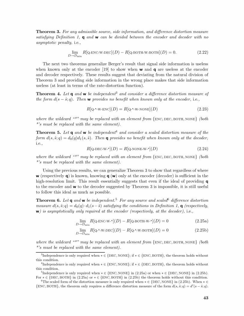
Theorem 3. For any admissible source, side information, and difference distortion measuresatisfying Definition 1, q and w can be divided between the encoder and decoder with no

asymptotic penalty, i.e.,

limD→Dmin

R[Q-ENC-W-DEC](D)−R[Q-BOTH-W-BOTH](D) = 0. (2.22)

The next two theorems generalize Berger’s result that signal side information is useless

when known only at the encoder [19] to show when w and q are useless at the encoderand decoder respectively. These results suggest that deviating from the natural division of

Theorem 3 and providing side information in the wrong place makes that side informationuseless (at least in terms of the rate-distortion function).

Theorem 4. Let q and w be independent3 and consider a difference distortion measure ofthe form d(s− s; q). Then w provides no benefit when known only at the encoder, i.e.,

R[Q-*-W-ENC](D) = R[Q-*-W-NONE](D) (2.23)

where the wildcard “*” may be replaced with an element from {ENC, DEC, BOTH, NONE} (both*’s must be replaced with the same element).

Theorem 5. Let q and w be independent4 and consider a scaled distortion measure of the

form d(s, s; q) = d0(q)d1(s, s). Then q provides no benefit when known only at the decoder,i.e.,

R[Q-DEC-W-*](D) = R[Q-NONE-W-*](D) (2.24)


Using the previous results, we can generalize Theorem 3 to show that regardless of wherew (respectively q) is known, knowing q (w) only at the encoder (decoder) is sufficient in the

high-resolution limit. This result essentially suggests that even if the ideal of providing qto the encoder and w to the decoder suggested by Theorem 3 is impossible, it is still useful

to follow this ideal as much as possible.

Theorem 6. Let q and w be independent.5 For any source and scaled6 difference distortionmeasure d(s, s; q) = d0(q) ·d1(s− s) satisfying the conditions in Definition 1, q (respectively,

w) is asymptotically only required at the encoder (respectively, at the decoder), i.e.,

limD→Dmin

R[Q-ENC-W-*](D)−R[Q-BOTH-W-*](D) = 0 (2.25a)

limD→Dmin

R[Q-*-W-DEC](D)−R[Q-*-W-BOTH](D) = 0 (2.25b)

where the wildcard “*” may be replaced with an element from {ENC, DEC, BOTH, NONE} (both

*’s must be replaced with the same element).

3Independence is only required when ∗ ∈ {DEC, NONE}; if ∗ ∈ {ENC, BOTH}, the theorem holds withoutthis condition.

4Independence is only required when ∗ ∈ {ENC, NONE}; if ∗ ∈ {DEC, BOTH}, the theorem holds withoutthis condition.

5Independence is only required when ∗ ∈ {ENC, NONE} in (2.25a) or when ∗ ∈ {DEC, NONE} in (2.25b).For ∗ ∈ {DEC, BOTH} in (2.25a) or ∗ ∈ {ENC, BOTH} in (2.25b) the theorem holds without this condition.

6The scaled form of the distortion measure is only required when ∗ ∈ {DEC, NONE} in (2.25b). When ∗ ∈{ENC, BOTH}, the theorem only requires a difference distortion measure of the form d(s, s; q) = d′(s− s; q).

43

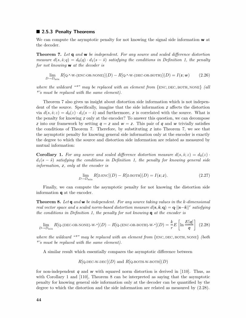
� 2.5.3 Penalty Theorems

We can compute the asymptotic penalty for not knowing the signal side information w atthe decoder.

Theorem 7. Let q and w be independent. For any source and scaled difference distortionmeasure d(s, s; q) = d0(q) · d1(s − s) satisfying the conditions in Definition 1, the penaltyfor not knowing w at the decoder is

limD→Dmin

R[Q-*-W-{ENC-OR-NONE}](D)−R[Q-*-W-{DEC-OR-BOTH}](D) = I(s;w) (2.26)

where the wildcard “*” may be replaced with an element from {ENC, DEC, BOTH, NONE} (all*’s must be replaced with the same element).

Theorem 7 also gives us insight about distortion side information which is not indepen-

dent of the source. Specifically, imagine that the side information z affects the distortionvia d(s, s; z) = d0(z) · d1(s − s) and furthermore, z is correlated with the source. What is

the penalty for knowing z only at the encoder? To answer this question, we can decomposez into our framework by setting q = z and w = z. This pair of q and w trivially satisfiesthe conditions of Theorem 7. Therefore, by substituting z into Theorem 7, we see that

the asymptotic penalty for knowing general side information only at the encoder is exactlythe degree to which the source and distortion side information are related as measured by

mutual information:

Corollary 1. For any source and scaled difference distortion measure d(s, s; z) = d0(z) ·d1(s − s) satisfying the conditions in Definition 1, the penalty for knowing general side

information, z, only at the encoder is

limD→Dmin

R[Z-ENC](D)−R[Z-BOTH](D) = I(s; z). (2.27)

Finally, we can compute the asymptotic penalty for not knowing the distortion side

information q at the encoder.

Theorem 8. Let q and w be independent. For any source taking values in the k-dimensional

real vector space and a scaled norm-based distortion measure d(s, s;q) = q·||s−s||r satisfyingthe conditions in Definition 1, the penalty for not knowing q at the encoder is

limD→Dmin

R[Q-{DEC-OR-NONE}-W-*](D)−R[Q-{ENC-OR-BOTH}-W-*](D) =k

rE

[

lnE[q]

q

]

(2.28)


A similar result which essentially compares the asymptotic difference between

R[Q-DEC-W-DEC](D) and R[Q-BOTH-W-BOTH](D)

for non-independent q and w with squared norm distortion is derived in [110]. Thus, aswith Corollary 1 and [110], Theorem 8 can be interpreted as saying that the asymptotic

penalty for knowing general side information only at the decoder can be quantified by thedegree to which the distortion and the side information are related as measured by (2.28).

44

According to Jensen’s inequality, this rate gap is always greater than or equal to zerowith equality if and only if q is a constant with probability 1. Furthermore, the rate gap

is scale invariant in the sense that it does not change when q is multiplied by any positiveconstant.

In Table 2.1, we evaluate the high-resolution rate penalty for a number of possible dis-

tributions for the side-information. Note that for all of these side information distributions(except the uniform and exponential distributions), the rate penalty can be made arbitrarily

large by choosing the appropriate shape parameter to place more probability near q = 0or q = ∞. In the former case (LogNormal, Gamma, or Pathological q), the large rate-lossoccurs because when q ≈ 0, the informed encoder can transmit almost zero rate while the

uninformed encoder must transmit a large rate to achieve high resolution. In the latter case(Pareto or Cauchy q), the large rate-loss is caused by the heavy tails of the distribution

for q. Specifically, even though q is big only very rarely, it is the rare samples of large q

which dominate the moments. Thus an informed encoder can describe the source extremelyaccurately during the rare occasions when q is large, while an uninformed encoder must

always spend a large rate to obtain a low average distortion.

Table 2.1. Asymptotic rate-penalty in nats. Euler’s constant is denoted by γ.

The rate penalties below are for not knowing distortion side information q at the encoderwhen distortion is measured via d(s, s; q) = q(s − s)2. (Multiply penalties in nats by

1/ ln 2 ≈ 1.44 to convert to bits).

Distribution Name Density for q Rate Gap in nats

Exponential τ exp(−qτ) − 12 ln γ ≈ 0.2748

Uniform 1q∈[0,1]12(1− ln 2) ≈ 0.1534

Lognormal 1

q√

2πQ2exp

[

− (ln q−M)2

2Q2

]Q2

4

Pareto ab

qa+1 , q ≥ b > 0, a > 1 12

[

ln aa−1 − 1/a

]

Gamma b(bq)a−1 exp(−bq)Γ(a)

12

{ln a− d

dx [ln Γ(x)]x=a

}≈ 1

2a

Pathological (1− ε)δ(q − ε) + εδ(q − 1/ε) 12 ln(1 + ε− ε2)− 1−2ε

2 ln ε ≈ 12 ln 1

ε

Positive Cauchy 2/π1+q2 , q ≥ 0 ∞

Finally, note that all but one of these distributions would require infinite rate to losslesslycommunicate the side information. This suggests that the gains in using distortion side

information are not obtained by exactly describing the side information to the receiver.

� 2.6 Finite Rate Bounds For Quadratic Distortions

So far we have shown that in the high-resolution limit, knowing q at the encoder is sufficient.Our main analytical tool was the additive test-channel distribution s = s + zq where the

additive noise in the test channel depends on the distortion side information. Evidently,additive test-channels of this type are asymptotically optimal. To investigate the rate-loss

45

at finite resolutions we develop two results for scaled quadratic distortion measures. Wealso briefly mention how these results can be generalized to other distortion measures.

� 2.6.1 A Medium Resolution Bound

Theorem 9. Consider a scaled quadratic distortion measure of the form d(s, s; q) = q · (s−s)2 with q ≥ qmin > 0. Then the maximum rate-gap at distortion D is bounded by

R[Q-ENC-W-DEC](D)−R[Q-BOTH-W-BOTH](D) ≤ J(s|w)

2·min

[

1,D

qmin

]

(2.29)

where J(s|w) is the Fisher Information in estimating a non-random parameter τ from τ + s

conditioned on knowing w . Specifically,

J(s|w)∆=

∫

pw(w)

{∫

ps|w (s|w)

[δ

δslog ps|w (s|w)

]2

ds

}

dw. (2.30)

Similar bounds can be developed with other distortion measures provided that D/qmin

is replaced with a quantity proportional to the variance of the quantization error. See theremark after the proof of Theorem 9 in the appendix for details.

One may wonder why Fisher Information appears in the above rate-loss bound. After

all, Fisher Information is most commonly used to lower bound the error in estimating aparameter via its use in the Cramer-Rao bound. What does Fisher Information have to dowith source coding?

To answer this question, recall that our bounds are all developed by using an additive

test-channel distribution of the form s = s + z. Thus, a clever source decoder could treateach source sample s [i] as a parameter to be “estimated” from the quantized representations [i]. If an efficient estimator exists, this procedure could potentially reduce the distortion by

the reciprocal of the Fisher Information. But if the distortion can be reduced in this mannerwithout affecting the rate, then the additive test-channel distribution must be sub-optimal

and a rate gap must exist.

So the bound in Theorem 9 essentially measures the rate gap by measuring how much

our additive test-channel distribution could be improved if an efficient estimator existed fors given s. This bound will tend to be good when an efficient estimator does exist and poor

otherwise. For example, if s is Gaussian with unit-variance conditioned on w , then theFisher Information term in (2.29) evaluates to one and the worst-case rate-loss is at mosthalf a bit at maximum distortion. This corresponds to the half-bit bound on the rate-loss

for the pure Wyner-Ziv problem derived in [193]. But if s is discontinuous (e.g., if s isuniform), then no efficient estimator exists and the bound in (2.29) is poor.

As an aside, we note that the proof of Theorem 9 does not require any regularityconditions. Hence, if the Fisher Information of the source is finite, it can be immediately

applied without the need to check whether the source is admissible according to Definition 1.

� 2.6.2 A Low Resolution Bound

While the Fisher Information bound from (2.29) can be used at low resolutions, it can be

quite poor if the source is not smooth. Therefore, we derive the following bound on therate-loss which is independent of the distortion level and hence most useful at low resolution.

46

Theorem 10. Consider a scaled quadratic distortion measure of the form d(s, s; q) = q ·(s− s)2 and denote the minimum/maximum conditional variance of the source by

σ2min = min

wVar [s|w = w] (2.31a)

σ2max = max

wVar [s|w = w] . (2.31b)

Then the gap in Theorem 3 is at most the conditional relative entropy of the source from a

Gaussian distribution plus a term depending on the range of the conditional variance:

R[Q-ENC-W-DEC](D)−R[Q-BOTH-W-BOTH](D) ≤ D(s|w ||N (Var [s])) +1

2log

(

1 +σ2

max

σ2min

)

(2.32)where N (t) represents a Gaussian random variable with mean zero and variance t.

Similar bounds can be developed for other distortion measures as discussed after theproof of Theorem 10 in the appendix.

Consider the familiar Wyner-Ziv scenario where the signal side information is a noisy

observation of the source. Specifically, let w = s + v where v is independent of s. In thiscase, the conditional variance is constant and (2.32) becomes

D(s|w ||N (Var [s])) +1

2log 2 (2.33)

and the rate-loss is at most half a bit plus the deviation from Gaussianity of the source.

If s is Gaussian when conditioned on w = w, then the rate-loss is again seen to beat most half a bit as in [193]. In contrast to [193] which is independent of the source,

however, both our bounds in (2.29) and (2.32) depend on the source distribution. Hence,we conjecture that our bounds are loose. In particular, for a discrete source, the worstcase rate loss is at most H(s|w), but this is not captured by our results since both bounds

become infinity. Techniques from [60,104,193] may yield tighter bounds.

� 2.6.3 A Finite Rate Gaussian Example

To gain some idea of when the asymptotic results take effect, we consider a finite rateGaussian example. Specifically, let the source consist of a sequence of Gaussian random

variables with mean zero and variance 1 and consider distortion side information withPr[q = 1] = 0.6, Pr[q = 10] = 0.4, and distortion measure d(s, s; q) = q · (s− s)2.

The case without side information is equivalent to quantizing a Gaussian random vari-

able with distortion measure 4.6(s − s)2 and thus the rate-distortion function is

R[Q-NONE-W-NONE](D) =

{

0, D ≥ 4.612 ln 4.6

D , D ≤ 4.6.(2.34)

To determine R[Q-BOTH-W-NONE](D) we must set up a constrained optimization as we did

for the binary-Hamming scenario in Appendix B.2. This optimization results in a “water-pouring” bit allocation which uses more bits to quantize the source when q = 10 than when

q = 1. Specifically, the optimal test-channel is a Gaussian distribution where both themean and the variance depend on q and thus s has a Gaussian mixture distribution. Going

47

through the details of the constrained optimization yields

R[Q-BOTH-W-NONE](D) =

0, 4.6 ≤ D0.42 ln 4

(D−.6) , D∗ ≤ D ≤ 4.60.42 ln 10

D + 0.62 ln 1

D , D ≤ D∗(2.35)

for some appropriate threshold D∗. Evaluating (2.28) for this case indicates that the rate-gap between (2.34) and (2.35) goes to 0.5 · (ln 4.6− 0.4 ln 10) ≈ 0.3 nats ≈ 0.43 bits.

Computing R[Q-ENC-W-NONE](D) analytically seems difficult. Thus, when distortion

side information is only available at the encoder we obtain a numerical upper bound onthe rate by using the same codebook distribution as when q is known at both encoder and

decoder. This yields a rate penalty of I (s; q).7 We can obtain a simple analytic boundfrom Theorem 9. Specifically, evaluating (2.29) yields that the rate penalty is at most(1/2) ·min[1,D].

In Fig. 2-8 we evaluate these rate-distortion trade-offs. We see that at zero rate, allthree rate-distortion functions have the same distortion since no bits are available for quan-

tization. Furthermore, we see that the Fisher Information bound is loose at zero rate. Asthe rate increases, the system with full distortion side-information does best because it usesthe few available bits to represent only the important source samples with q = 10. The de-

coder reconstructs these source samples from the compressed data and reconstructs the lessimportant samples to zero (the mean of s). In this regime, the system with distortion side

information at the encoder also more accurately quantizes the important source samples.But since the decoder does not know q, it does not know which samples of s to reconstructto zero. Thus the system with q available at the encoder performs worse than the one with

q at both encoder and decoder but better than the system without side information. Asthe rate increases further, both systems with distortion side information quantize source

samples with both q = 1 and q = 10. Thus the codebook distribution for s goes froma Gaussian mixture to become more and more Gaussian and the rate-loss for the systemwith only encoder side information goes to zero. Finally, we note that even at the modest

distortion of −5 dB, the asymptotic effects promised by our theorems have already takeneffect.

� 2.7 Discussion

In this chapter, we introduced the notion of distortion side information which does notdirectly depend on the source but instead affects the distortion measure. Furthermore, weshowed that if general side information can be decomposed into such a distortion dependent

component and a signal dependent component then under certain conditions the former isrequired only at the encoder and the latter is required only at the decoder. In this section,

we discuss some implications and applications of these ideas.

� 2.7.1 Applications to Sensors and Sensor Networks

There is a growing interest in sensor networks where multiple nodes with potentially corre-

lated observations cooperate to sense the environment. A variety of researchers have already

7Actually, since the rate distortion function is convex, we take the lower convex envelope of the curveresulting from the optimal test-channel distribution.

48

Figure 2-8. Rate-distortion curves for quantizing a Gaussian source s with distortion q(s − s)2 where theside information q is 1 with probability 0.6 or 10 with probability 0.4. From bottom to top on the rightthe curves correspond to the rate required when both encoder and decoder know q, a numerically computedupper bound to the rate when only the encoder knows q, the rate when neither encoder nor decoder knowq, and the Fisher Information upper bound from Theorem 9 for when only the encoder knows q.

49

demonstrated the advantages of distributed source coding in efficiently using signal side in-formation in such networks [149, 146, 136, 175, 21]. We believe, however, that the possible

applications of distributed coding with distortion side information are equally compelling.

First, many sensors naturally receive distortion side information in addition to the ob-served signal. For example, sensors which perform simple filtering or averaging of the

incoming signal can use the variance as an indicator of reliability. Similarly, sensors canobserve the background level of light, sound, etc., to obtain an estimate of the noise-floor in

the absence of a signal of interest. Since the level of this noise-floor may change over time,such background noise readings can be used as an estimate of signal reliability.

Second, many sensors must be periodically re-calibrated either by manual intervention,

with automatic self-calibration routines, or by communicating with other sensors. Thelength of time since the last calibration or an estimate of the calibration accuracy are thus

natural measures of reliability for the observations. For example, many systems are designedto record data at a roughly constant average amplitude. This is often accomplished by usingautomatic gain control (AGC) to compensate for attenuation due to distance, weather,

or obstacles. Since thermal noise in the sensor front-end is usually independent of suchattenuations, the AGC level can be used as a simple indicator of the signal-to-noise ratio

of an observed signal.

In more sophisticated systems, intermediate nodes or fusion centers may collect data

and perform various levels of processing. These fusion centers can often form preliminaryestimates of the value of different components of the data. These estimates can the be usedas distortion side information in deciding the accuracy used to further communicate or store

the processed data.

In all these cases, our results suggest that trying to communicate distortion side in-

formation along with the signal is often not the right way to design a system. Instead,compression schemes should be designed such that the decoder is in some sense invariantto the side information. Of course, the encoder must still be able to more accurately repre-

sent the important or reliable data. As illustrated by the examples in Section 2.2, varioustransforms may play a role in achieving this goal.

� 2.7.2 Richer Distortion Models and Perceptual Coding

Notion of distortion side information may be particularly useful in the design of perceptualcoders. Specifically, it is well-known that mean-square error is at best a poor representative

of how humans experience distortion. Hence perceptual coding systems use features ofthe human visual system (HVS) or human auditory system (HAS) to achieve low subjective

distortion even when the mean-square distortion is quite large. Unfortunately, creating sucha perceptual coder often requires the designer to be an expert both in human physiology,as well as quantizer design. This difficulty may be one of the reasons why information

theory has sometimes had less impact on compression standards than on communicationstandards.

Using the abstraction of distortion side information to represent such perceptual effects,however, may help overcome this barrier. For example, physiological experts could focus onproducing a distortion model which incorporates perceptual effects by determining a value

qi which scales the quadratic distortion between the ith source sample and its reconstruc-tion. Quantization experts could focus on designing compression systems operating with

distortion side information. Then various perceptual models could be quickly and easilycombined with quantizer designs to find the best combination. This modular design would

50

allow a good quantization system to be used in a variety of application domains simply bychanging the model for the distortion side information. Similarly, it would allow a finely

tuned perceptual model to be used in many types of quantizer designs.

The theoretical justification for using distortion side information to design modular

quantizers is Theorem 3. This theorem can be interpreted as saying that even if the per-ceptual model which produces the distortion weighting qi is a complicated function of thesource, the decoder does not need to know how the perceptual model works. Instead, it is

sufficient for the decoder simply to know the statistics of q provided that q is available tothe encoder.

Finally, it may be somewhat premature to advocate a particular design for perceptualcoders based on primarily on rate-distortion results. At a minimum, however, we point outthat if a perceptual distortion side information model can be constructed it can at least be

used to find a bound on the minimum possible bit rate at a given distortion. Having sucha performance benchmark to strive for can be a powerful force in inspiring system designer

to search for new innovations.

� 2.7.3 Decomposing Side Information Into q and w

Our problem model of Section 2.3 requires that the side information can be decomposedinto distortion side information and signal side information. In many scenarios, this maybe a natural view of the compression task. In problems where this is not the case, however,

we briefly discuss how general side information may be decomposed into the pair (q,w)required by our theorems.

First, notice that the formulation in (2.1) is completely general in the sense that anyside information z taking values in the set Z can be trivially decomposed into (q,w) by

setting (q,w) = (z, z) with (Q,W) = (Z,Z). Of course, this makes most of our resultsuninteresting. One systematic procedure for potentially improving this decomposition isas follows. First, replace each pair of values (q0, q1) where d(·, ·; q0) = d(·, ·; q1) with a

new value q′ and adjust Q accordingly. Next, replace each pair of values (w0, w1) whereps|w (·|w0) = ps|w (·|w1) and pq|w(·|w0) = pq|w(·|w1) with a new value w′ and adjust Waccordingly. If the resulting Q and W are smaller than Z, then our results become non-trivial.

As with the problem of determining a minimal sufficient statistics, there are many

potential decompositions and different notions of good decompositions may be appropriatein different applications. For example, minimizing the cardinality of Q, W, or both, might

be useful in simplifying quantizer design or related tasks. Alternatively, minimizing I(q;w),H(q), H(w), or similar information measures may be useful if q/w must be communicatedto the encoder/decoder by a third party.

Essentially, all that a side information decomposition, requires for our results to hold aretwo Markov conditions. First, we need the Markov condition q↔ w↔ s. Second, if we view

the distortion as a random variable d(s, s) which can depend on the side information, weneed the Markov condition d(s, s)↔ q, s, s↔ w. In some scenarios, natural decompositions

exist which satisfies these conditions, but finding a general procedure to obtain the best suchdecomposition is a topic for future work.

51

� 2.8 Concluding Remarks

Our analysis indicates that side information which affects the distortion measure can pro-vide significant benefits in source coding. Perhaps, our most surprising result is that in a

number of cases, (e.g., sources uniformly distributed over a group, or in the high-resolutionlimit) side information at the encoder is just as good as side information known at bothencoder and decoder. Furthermore, this “separation theorem” can be composed with the

previously known result that having signal side information at the decoder is often as goodas having it both encoder and decoder (e.g., in the high-resolution limit). Our main results

regarding when knowing a given type of side information at one place is as good as knowingit at another place are summarized in Fig. 2-7. Also, we computed the rate-loss for lackinga particular type of side information in a specific place. These penalty theorems show that

lacking the proper side information can produce arbitrarily large degradations in perfor-mance. Taken together, we believe these results suggest that distortion side information is

a useful source coding paradigm.

� 2.8.1 Possibilities For Future Work

Many practical, theoretical, and modeling issues remain to be explored in the study of

distortion side information.Probably the most pressing modeling issue is the investigation and development of useful

distortion side information measures. A standard model (or class of models) for distortionside information in various applications would be invaluable in addressing semantic aspectsof distortion ignored by cruder measures such as squared or absolute error. Developing

such models may be a lengthy, expensive, and even controversial task. Similar difficultiesare encountered in developing channel models for many wired and wireless communication

applications, yet the value of such models makes them an active area of research.Besides modeling questions, an interesting practical issue is the construction of low com-

plexity quantizers which can approach the theoretical advantages of distortion side informa-

tion in real systems. Some possibilities include investigating low dimensional quantizers viaLloyd-Max algorithms, lattice quantizers or companding. High dimensional constructions

based on sophisticated codes may also prove useful if low complexity encoding and decodingalgorithms can be constructed.

On the theoretical side, some interesting questions include the benefits of distortion side

information in scalable or distributed source coding problems, the theory of distortion sideinformation for non-difference distortion measures, and multiple description coding with

distortion side information.

52

Chapter 3

Low Complexity Quantizers ForDistortion Side Information

53


Most classical work on lossy data compression and source coding focuses on encoding asource into a compressed representation such that compressed version is “close” to the orig-inal as measured by some distortion function. Choosing an accurate distortion measure

is critical. Unfortunately, however, sophisticated distortion measures are often difficult towork with in analysis and design. Thus one common model is to measure the distortion be-

tween a length n source sequence, s [n1 ], and its quantized reconstruction, s [ n

1 ], by averaginga single-letter distortion measure, i.e.

d(s [n1 ] , s [n

1 ]) =1

n

n∑

i=1

d(s [i] , s [i]). (3.1)

Single-letter distortion measures have led to a number of theoretical insights and practi-cal advances, but they seem to miss a key feature of many problems. For example, considera sensor application with the observations s [ n

1 ]. Furthermore, imagine that each observation

is made with a different reliability or signal-to-noise ratio (SNR). When s [ n1 ] is quantized

to s [n1 ], our intuition suggests that the high reliability or high SNR observations should be

treated differently than the low reliability or low SNR ones. As another example, considerthe encoding of speech, audio, or video. It is well-known that due to perceptual effects, cer-tain components of such signal may be more or less sensitive to distortion due to masking

effects or context [85]. For example errors in audio samples following a loud sound, or errorsin pixels spatially or temporally near bright spots are perceptually less relevant. Similarly,

accurately preserving certain edges or textures in an image or human voices in audio maybe more important than preserving background patterns/sounds.

To model some of these effects in, we introduced the idea of distortion side informationin Chapter 2. Specifically, we considered quantizing a source s [ n

1 ] into s [n1 ] subject to a

distortion measure which depends on the side information q [n1 ] via

d(s [n1 ] , s [n

1 ] ; q [n1 ]) =

1

n

n∑

i=1

d(s [i] , s [i] ; q [i]). (3.2)

Intuitively, the distortion side information q [i] represents information such as the SNR ofthe ith source sample, the perceptual distortion masking, or other effects which make somecomponents of a signal more or less important. Some possibilities for how the distortion side

information might weight or otherwise modify the distortion measure on a sample-by-samplebasis include single-letter distortion measures such as d(s [i] , s [i] ; q [i]) = q [i] · (s [i]− s [i])2

or d(s [i] , s [i] ; q [i]) = |s [i]− s [i] |q[i].

By allowing this richer class of distortion measures, we can more accurately representthe goals of a lossy compression system. Presumably, such accuracy should lead to betterperformance. For example, in a fully informed system where q [n

1 ] is known to both encoder

and decoder, this distortion side information could be used to allocate more bits to sensitivesamples indicated by q [i]. This intelligent bit allocation should outperform an uniformed

system where all source samples are treated the same.

But what happens for a partially informed system where only the encoder knows q [ n1 ]?

For example, in a sensor scenario it might be reasonable to model the encoder as having

access to the SNR for each observation, but the receiver or decoder might not have suchknowledge. Therefore, at first it might seem like the added benefit for a sophisticated

54

distortion model would be outweighed by the need for the encoder to convey q [ n1 ] to the

decoder. In Chapter 2, we show that this is often not the case. Specifically, we show that

in many cases of interest it is possible for the partially informed system where only theencoder knows q [n

1 ] to obtain the same performance as the fully informed system whereboth encoder and decoder know q [n

1 ]. Thus, in many cases we can gain the full benefit

of sophisticated distortion side information models without the need to explicitly transmitq [n

1 ] from the encoder to the decoder.

While the results in Chapter 2 use random coding arguments, in this chapter we pro-

pose a constructive, practically implementable method to use distortion side information.Specifically, we describe lattice based lossy compression systems to exploit distortion side

information known only at the encoder. We show that the proposed systems gain thefull benefit of the distortion side information while requiring complexity which grows onlylinearly with the block length, n.

We focus on lattice based systems followed by entropy coding for a number of reasons.

From a practical perspective, lattices have many advantages for source coding (see, e.g.,[78, 58, 117, 112, 41, 40, 130, 86, 197]). Indeed, an integer lattice followed by entropy coding

is one of the most commonly used lossy compression systems. Furthermore, many resultsexists on constructing, encoding/decoding, analyzing, and using lattices such as [198,64,63,165,153,2,200,168,111,177,131]. Finally, lattices are a useful tool in analyzing the different

types of gains possible in lossy compression. For example, [112] identifies the space-fillinggain, shape gain, and memory gain as separate possible gains to pursue. Similarly, for

high-rate quantizers, [58] identifies the granular gain and boundary as gains which can beachieved separately via lattices.

Essentially, we continue along these lines by introducing a type of transform across

nested lattices and showing that this transform obtains the full benefit of the distortion sideinformation. Thus the distortion side information gain is separate from both the boundarygain achieved by entropy coding and the granular gain achieved by selecting an appropriate

sequence of nested lattices.

The rest of this chapter is organized as follows. We begin with some simple examplesin Section 3.2 which convey the key insights of this chapter. These examples show how

to design partially informed systems where only the encoder knows the distortion sideinformation. Furthermore, these examples demonstrate that partially informed systems can

achieve the same performance as fully informed systems where both encoder and decoderknow the distortion side information. Next, we briefly establish some notation in Section 3.3.Section 3.4 presents our constructions for how lattice based quantizers which efficiently

exploit distortion side information. While Section 3.4 focuses on the quantizer structureand codebook format, Section 3.5 we describes a sub-optimal but provably efficient encoding

algorithm. Specifically, in Section 3.5.1 we describe the rule for mapping source and sideinformation into the format specified in Section 3.4. Then in Section 3.5.3, we show that theproposed rule can be implemented with linear complexity. After introducing a statistical

model for the source and side information in Section 3.5.4, we derive the rate-distortionperformance for our proposed encoding rule in Section 3.5.6 and show that it matches the

rate-distortion performance of the fully informed system in Section 3.5.5. We close withsome concluding remarks in Section 3.6.

55

� 3.2 Two Simple Examples

We illustrate some different ways distortion side information can be efficiently used even

when known only at the encoder.

� 3.2.1 Discrete Uniform Source

Consider the case where the source, s [i], corresponds to n samples each uniformly and in-

dependently drawn from the finite alphabet S with cardinality |S| ≥ n. Let q [i] correspondto n binary variables indicating which source samples are relevant. Specifically, let thedistortion measure be of the form d(s, s; q) = 0 if and only if either q = 0 or s = s. Finally,

let the sequence q [i] be statistically independent of the source with q [i] drawn uniformlyfrom the n choose k subsets with exactly k ones.

If the side information were unavailable or ignored, then losslessly communicating thesource would require exactly n · log |S| bits. A better (though still sub-optimal) approach

when encoder-only side information is available would be for the encoder to first tell thedecoder which samples are relevant and then send only those samples. This would require

n · Hb(k/n) + k · log |S| bits where Hb(·) denotes the binary entropy function. Note thatwhen the side information is known at both encoder and the decoder, then the overhead

required in telling the decoder which samples are relevant could be avoided and the totalrate required is exactly k · log |S|. We will show that this overhead can in fact be avoidedeven without decoder side information.

Pretend that the source samples s [0], s [1], . . ., s [n− 1], are a codeword of an (n, k)

Reed-Solomon (RS) code (or more generally any MDS1 code) with q [i] = 0 indicating anerasure at sample i. Use the RS decoding algorithm to “correct” the erasures and determine

the k corresponding information symbols which are sent to the receiver. To reconstruct thesignal, the receiver encodes the k information symbols using the encoder for the (n, k) RScode to produce the reconstruction s [0], s [1], . . ., s [n− 1]. Only symbols with q [i] = 0

could have changed, hence s [i] = s [i] whenever q [i] = 1 and the relevant samples arelosslessly communicated using only k · log |S| bits.

As illustrated in Fig. 3-1, RS decoding can be viewed as curve-fitting and RS encodingcan be viewed as interpolation. Hence this source coding approach can be viewed as fitting

a curve of degree k − 1 to the points of s [i] where q [i] = 1. The resulting curve can bespecified using just k elements. It perfectly reproduces s [i] where q [i] = 1 and interpolates

the remaining points.

Figure 3-1. Losslessly encoding a source with n = 7 points where only k = 5 points are relevant (i.e., theunshaded ones), can be done by fitting a fourth degree curve to the relevant points. The resulting curve willrequire k elements (yielding a compression ratio of k/n) and will exactly reproduce the desired points.

1The desired MDS code always exists since we assumed |S| ≥ n. For |S| < n, near MDS codes existwhich give asymptotically similar performance with an overhead that goes to zero as n →∞.

56

� 3.2.2 Weighted Quadratic Distortion

The previous example in Section 3.2.1 can be generalized to Gaussian sources with quadraticdistortion. Specifically, provided that d(·, ·; q) = 0 whenever q = 0 and is otherwise inde-

pendent of q, then the technique in Section 3.2.1 can be generalized by replacing MDS codeswith Fourier Transforms [124]. This requires a very special form for the distortion measureand may be of limited interest. In the rest of this section, we consider another example

which illustrates how distortion side information may be used for a much wider range ofdistortion measures.

Consider quantizing a pair of source samples (s [1] , s [2]) subject to the distortion con-

straint d(s, s; q) = q · (s− s)2. Furthermore, imagine that the distortion side information issuch that one source sample is sixteen times more important than the other. Specifically, let

(q [1] , q [2]) = (1, 16) or (q [1] , q [2]) = (16, 1). In the following we consider how to designhigh-resolution quantizers when q is known at both encoder and decoder as well as when q

is known only at the encoder.

Encoder & Decoder Know q

For the moment, let us restrict attention to simple uniform scalar quantizers followed byentropy coding. If both encoder and decoder know the distortion side information, then the

optimal strategy is straightforward: use a quantizer step-size of ∆ for the more importantsource sample and a step-size of 4∆ for the less important sample.

Fig. 3-2 illustrates this idea for quantizing two source samples, s [1] and s [2]. If the firstsource sample is more important (i.e., q [1] = 16 and q [2] = 1), then a denser quantizeris used for the first source sample and a coarser quantizer is used for the second source

sample. If the second source sample is more important, the situation is reversed.

It is well-known that in the limit of small distortions, the average squared error for astep-size ∆ uniform scalar quantizer is simply the variance of random variable uniformly

distributed over the interval (0,∆). Thus the expected distortion is approximately 16·∆2/12for the more important sample and (4∆)2/12 = 16 · ∆2/12 (i.e., the same) for the less

important sample.

Provided that the source has a probability density function, it is straightforward to showthat total number of bits required by the two quantizers is approximately

h(s)− log∆ + h(s)− log 4∆ (3.3)

for a total average bit rate ofh(s)− log 2∆ (3.4)

bits per sample.

Essentially, using a fine-grained quantizer for the more important sample and a coarse-

grained quantizer for the less important sample is like using a variable codebook and par-tition as illustrated in Fig. 3-3. Specifically, the codebook and partition in Fig. 3-3(a)correspond to the quantizer in Fig. 3-2(a) while the codebook and partition in Fig. 3-3(b)

correspond to Fig. 3-2(b). In each case, the codebook and partition are designed to mini-mize the error in quantizing the more important sample. Note that, Fig. 3-3 illustrates that

the decoder must know the distortion side information to know which point set to use inmapping a quantization index to a reconstruction of the source.

57

PSfrag replacements

s [1]

s [2]

s [1]

s [2]

(a)

PSfrag replacements

s [1]

s [2]

s [1]

s [2]

(b)

Figure 3-2. Two possible quantizers to use if both the encoder and decoder know the distortion sideinformation. When the first source sample, s [1], is more important as in (a), then a finer quantizer is usedfor it and a coarser quantizer is used for s [2]. In (b), the second source sample, s [2] is more important andthus the situation is reversed.

Only Encoder Knows q

How can we achieve similar performance when only the encoder knows the distortion side

information? Ideally we wish to spend two extra bits on each sample where q [i] = 16since these samples require more accurate description than samples with q [i] = 1. A naive

approach in achieving this goal would be for the encoder to first use 1 bit per sample totell the decoder whether or not a sample is important. Once this is accomplished thenthe structures in Figures 3-2 and 3-3 can be used. Of course, explicitly sending an extra

bit to indicate whether a sample is important or not incurs an overhead which is notrequired when both encoder and decoder know q. This overhead makes the naive approach

undesirable. Hence, we describe a system which can allocate two more bits of descriptionto each important sample without requiring any overhead.

Our approach is to use a pair of shifted quantizers. We again use an example with twosource samples. The encoder quantizes both source samples with a pair of quantizers of step-

size 4∆. The corresponding reconstructions are shifted by an offset of λ ∈ {0,∆, 2∆, 3∆}.The same offset is used for both quantizers. Thus the total number of bits required arethe same as the fully informed system. Specifically, approximately h(s) − log 4∆ bits are

required to quantize each source sample to a grid of step-size 4∆ plus an additional twobits to specify the shift λ ∈ {0,∆, 2∆, 3∆}. Thus the total average bit rate is the same as

(3.4). The shift is chosen to minimize the error for the more important sample (i.e., theone for which q [i] = 16). Using shifted quantizers in this manner has the effect of devoting

58

��

��

��

��

��

��

��

��

��

��

��

��

��

��

��

��

!!

""##

$$%%

&&''

(())

**++

,,--

..//

0011

2233

4455

PSfrag replacements

s↑

→

(a)

6677

8899

::;;

<<==

>>??

@@AA

BBCC

DDEE

FFGG

HHII

JJKK

LLMM

NNOO

PPQQ

RRSS

TTUU

VVWW

XXYY

ZZ[[

\\]]

^^__

``aa

bbcc

ddee

ffgg

hhii

jjkk

llmm

nnoo

ppqq

rrss

ttuu

vvww

PSfrag replacements

s

↑

→

(b)

Figure 3-3. Variable codebook and partition view of the quantizers in Fig. 3-2 obtained by grouping thetwo samples into a vector s = (s [1] , s [2]). If the distortion side information indicates s [1] is more importantthen the codebook and partition in (a) are used, while if the second sample is more important then (b) isused.

the extra two bits of information to describing the important sample without the need forthe overhead required to describe which sample is important.

Fig. 3-4 illustrates this idea. In Fig. 3-4(a), a quantizer of step-size 4∆ is used for bothsamples. By using an additional 2 bits to specify a shift of λ = 3∆ for the first sample,

however, we are effectively able to use 2 more bits for the important sample and achieveboth the same average rate and distortion as the fully informed system in Fig. 3-2(a).Alternatively, if the second source sample is important as in Fig. 3-4(b), the shift is chosen

to minimize the error in quantizing s [2] and we are again able to use 2 more bits for theimportant sample to achieve the same average rate and distortion as the fully informed

system in Fig. 3-2(b).

Essentially, the idea of using a pair of quantizers with a single shift applied to both is

like using a single, fixed set of codewords with a variable partition as illustrated in Fig. 3-5.Specifically, the partition in Fig. 3-5(a) corresponds to the quantizer in Fig. 3-4(a) while the

partition in Fig. 3-5(b) corresponds to the quantizer in Fig. 3-4(b). In each case, the locationof the points (i.e., the codebook) is fixed while it is only the partition that changes. Thepartition depends on the distortion side information in the sense that the encoder finds the

“nearest” quantization point where “nearest” depends on the distortion side information.Once the encoder has chosen the best quantization point and described it to the decoder,

the decoder can produce a quantized reconstruction of the source without knowing thedistortion side information.

59

PSfrag replacements

s [1]

s [2]

s [1]

s [2]

s [1] + λ

s [2] + λ

(a)

PSfrag replacements

s [1]

s [2]

s [1]

s [2]

s [1] + λ

s [2] + λ

(b)

Figure 3-4. Two possible quantizers to use if only the encoder knows the distortion side information. Thestructure in (a) is used if the first sample is more important and (b) is used if the second sample is moreimportant. In either case, each source sample is quantized to a grid of size 4∆ represented by the wide tickmarks. Next, both reconstructions are shifted by an offset, λ ∈ {0, ∆, 2∆, 3∆}, where ∆ corresponds to thefine spacing between narrow tick marks. When the first source sample, s [1], is more important as in (a),s [1] is quantized to the bottom wide tick mark and an offset of λ = 3∆ is selected. The error of the resultingreconstruction, s [1] + λ, essentially corresponds to the fine grid size, ∆. Conversely, the less importantsample is quantized to the second wide tick mark from the top so that the resulting error is proportional tothe coarse grid size, 4∆. The situation is reversed in (b) where the second source sample is more importantand thus a shift of λ = ∆ is selected to minimize the error in quantizing s [2].

� 3.3 Notation

Vectors are denoted in bold (e.g., x). The ith element of a sequence is denoted as x [i]if it is scalar or x [i] if it is a vector. Similarly, a subsequence of elements ranging from i

to j is denoted as x [ ji ] for sequences of vectors or x [ j

i ] for sequences of scalars. Randomvariables are denoted using the sans serif font (e.g., x) while random vectors are denotedwith bold sans serif (e.g., x). We denote mutual information, entropy, and expectation

as I(x ; y), H(x), E[x ]. Calligraphic letters denote sets (e.g., s ∈ S) with | · | denotingthe cardinality of its argument. Finally, for any length n sequence q [ n

1 ], we denote the

number of occurrences of the symbol i as #[q [n1 ] ∼ i]. In the Information Theory literature,

#[q [n1 ] ∼ i] is sometimes refereed to as the type of q [ n

1 ].

� 3.4 Lattice Quantizer Structures

In this section we describe how to generalize the construction in Section 3.2 to a widevariety of source and distortion measures. Specifically, our main goal is to construct efficient

60

��

��

��

��

��

��

��

��

��

��

��

��

��

��

��

��

!!

""##

$$%%

PSfrag replacements

s↓

(a)

&&''

(())

**++

,,--

..//

0011

2233

4455

6677

8899

::;;

<<==

>>??

@@AA

BCBBCBDD

EEFF

GGHH

ICIICIJJ

KKLL

PSfrag replacements

s →

(b)

Figure 3-5. A fixed codebook/variable partition view of the quantizers in Fig. 3-4 obtained by groupingthe two source samples into a vector s = (s [1] , s [2]). If the distortion side information indicates s [1] is moreimportant then the partition in (a) is used, while if the second sample is more important then partition (b)is used. In either case, the source is mapped to the codeword which minimizes the average error weightedby the distortion side information. Note that while in Fig. 3-3 both the partition and codebook change as afunction of the distortion side information, here only the partition depends on the side information and thelocation of the points (i.e., the codebook) is fixed.

quantizers when the distortion side information is known only at the encoder. In measuring

efficiency, we will compare a partially informed system where only the encoder knows thedistortion side information to a fully informed system where both encoder and decoderknow the distortion side information. An efficient partially informed system is one which

either exactly or asymptotically achieves the same performance as the corresponding fullyinformed system.

We consider a quantizer or lossy compression system to consist of an encoder and decoder

which work as follows. The encoder is presented with a length n source sequence s [ n1 ] and

a length n distortion side information sequence q [ n1 ]. The encoder produces an index which

is stored or transmitted to a decoder. In a fully informed system, the decoder receives boththe encoder output as well as q [ n

1 ]. In a partially informed system the decoder receivesthe index but does not know q [ n

1 ]. In either case, the error for the reconstruction s n1 is

computed by averaging the single-letter distortion measure, d(·, ·; ·), to obtain

d(s [n1 ] , s [n

1 ] ; q [n1 ]) =

1

n

n∑

i=1

d(s [i] , s [i] ; q [i]). (3.5)

The key insight in developing the example in Section 3.2.2 is the implicit use of a coset de-composition. Specifically, we used the fact that the integer lattice, Z = {. . . ,−2,−1, 0, 1, 2, . . .},can be decomposed into four shifts of the sub-lattice of integers which are multiples of four,4Z = {. . . ,−8,−4, 0, 4, 8, . . .}. Both the fully informed system in Section 3.2.2 and the par-

61

tially informed system in Section 3.2.2 were constructed by essentially using the Z lattice toquantize the more important sample and using the 4Z lattice to quantize the less important

sample. Hence, to develop quantizers which can efficiently use encoder side information fora variety of sources and distortion measures, we develop quantizers based on lattices. Webegin by briefly reviewing some lattice terminology. Further details on lattices can be found

in [63,41].

� 3.4.1 A Brief Review of Lattices and Cosets

A real, r-dimensional lattice, Λ ⊂ Rr, is a regular array of points in space which forms

a group under vector addition.2 The nesting idea used in Section 3.2.2 can be captured

by sub-lattices. Specifically, a sub-lattice Λ′ ⊂ Λ is any subgroup of Λ with respect tovector addition. We refer to a sequence of sub-lattices Λ(1) ⊂ Λ(2) ⊂ . . . ⊂ Λ(L) of

the base lattice Λ(L) as a nested lattice. Throughout the chapter, the reader may find ituseful to keep in mind integer nested lattices as a concrete embodiment of a nested lattice.Specifically, let Λ(j) be integer multiples of 2L−j . Thus Λ(L) is simply the integers Z =

{. . . ,−2,−1, 0, 1, 2, . . .}, Λ(L − 1) consists of even integers 2Z = {. . . ,−4,−2, 0, 2, 4, . . .},Λ(L− 2) consists of multiples of four, 4Z, and so on.

For a pair of lattices Λ′ ⊂ Λ, we denote the partition of Λ into equivalence classesmodulo Λ′ as Λ/Λ′. By taking one element from each equivalence class we obtain a system

of coset representatives denoted by [Λ/Λ′]. By using a coset decomposition for the partitionwe can uniquely specify a point λ in the base lattice Λ by the sum λ′ + c where λ′ is an

element of the sub-lattice Λ′ and c is the coset representative in [Λ/Λ′]. For the examplewhere Λ(L) = Z and Λ(L− 1) = 2Z, we can choose [Λ(L)/Λ(L− 1)] = {0, 1}. This allowsus to represent any integer z ∈ Z as z = e + c where e is an even integer and c ∈ {0, 1}.

We can continue this idea further. Instead of the representation

Λ(L) = Λ(L− 1) + [Λ(L)/Λ(L− 1)] (3.6a)

where any element in Λ(L) is described by an element of Λ(L−1) and a coset representative

in [Λ(L)/Λ(L− 1)], we can use the further decomposition

Λ(L− 1) = Λ(L− 2) + [Λ(L− 1)/Λ(L− 2)]. (3.6b)

Combining (3.6a) and (3.6b) yields the representation

Λ(L) = Λ(L− 2) + [Λ(L− 1)/Λ(L− 2)] + [Λ(L)/Λ(L− 1)]. (3.6c)

For example, setting Λ(L) = ∆Z, with Λ(L − 1) = 2∆Z and Λ(L − 2) = 4∆Z yields thedecomposition used in Section 3.2.2. Specifically, to describe an element of a grid of step-size ∆, we can instead describe an element of a grid of step-size 4∆ plus an element from

{0,∆} plus an element from {0, 2∆}. Taken to its conclusion this notation allows us to usethe partition chain

Λ(L)/Λ(L− 1)/ . . . /Λ(1) (3.7)

to represent any element of Λ(L) with an element of Λ(1) combined with the L − 1 cosetrepresentatives from each partition.

2For simplicity we focus on lattices, but most of our constructions and analysis only require the groupproperty and some notion of uniformity such as [65]. Thus, our ideas can be easily extended to other spacessuch as quantizing phases or angles.

62

� 3.4.2 The Fully Informed System

First we consider a fully informed system for quantizing the source sequence s [ n1 ] where

each source sample, s [i], is an r-dimensional vector. The fully informed system is designedto treat L different kinds of samples (e.g., if q takes exactly L different values) and consists

of a sequence of r-dimensional nested lattices

Λ(1) ⊂ Λ(2) ⊂ Λ(3) ⊂ . . . ⊂ Λ(L). (3.8)

Intuitively, the finest lattice Λ(L) is used to quantize the most important samples, whilethe coarser lattice, Λ(L− 1), is used for the next most important class of samples, and so

on until Λ(1) is used for the least important samples.

To quantize a source sequence s [ n1 ], we first classify each source sample, s [i], into one

of L classes according to the value of q [i]. For example, if q ∈ {1, 2, . . . , L}, we can simplyrepresent the class for s [i] by the value of q [i]. To simplify the exposition we assume that

this is the case. 3 Then s [i] is quantized to the nearest point in lattice Λ(q [i]), which werepresent as λΛ(q[i])(i). Finally, the resulting quantization indexes are entropy coded and

described to the receiver. The system described in Section 3.2.2 is one example of a fullyinformed system where L = 2, Λ(2) = ∆Z, Λ(1) = 4∆Z, and d(s, s; q) = q4 · (s− s)2.

� 3.4.3 The Partially Informed System

To facilitate comparison, we construct a partially informed system using the same latticeand lattice partition chain as for the fully informed system. Specifically, our basic tool is a

sequence of L r-dimensional nested lattices as in (3.8). Our goal is to match the performanceof the corresponding fully informed system described in Section 3.4.2. Note that one simpleand sub-optimal approach would be for the encoder to simply send q [ n

1 ] to the decoder and

then use the quantizer for the fully informed system. This would incur an overhead of H(q)bits per sample. Instead, we describe a quantizer which uses the same lattices as the fully

informed system in a somewhat different manner in order to avoid the overhead of H(q)required in communicating q.

Codebook Structure and Decoding

To quantize the source sequence s [ n1 ] with the distortion side information q [n

1 ], the encodersends three different pieces of information:

1. A list of the number of samples in q [ n1 ] taking the value i (denoted as #[q [n

1 ] ∼ j])

2. A sequence of n elements from the coarsest lattice Λ(1) (this sequence is denoted

λΛ(1)(i) with i ∈ {1, 2, . . . , n})

3. A table of coset representatives, c[i, j], where c[i, j] is the coset representative for thepartition [Λ(j + 1)/Λ(j)] for sample i with i ∈ {1, 2, . . . , n} and j ∈ {1, 2, . . . , L− 1}

Postponing for the moment how each of these components is determined and efficientlyencoded, once this encoding of the source s [ n

1 ] is received, the decoder reconstructs the

3Instead, if the number of possible values of q [i] is large or if q takes values in a continuum, then a morecomplicated classifier may be required. In such cases, we could transform the original problem into one witha new type of distortion side information, q′, and a new distortion measure where there are only L possiblevalues for q′. Hence our assumption incurs no essential loss of generality but simplifies notation.

63

sequence s [n1 ] by setting

s [i] = λΛ(1)(i) +

L−1∑

j=1

c[i, j]. (3.9)

Encoding #[q [n1 ] ∼ j]

The number of occurrences of the sample j in q [ n1 ] can be encoded by via entropy coding

(e.g., Huffman coding or Arithmetic coding) if a statistical characterization of q is available.

Even without any statistical characterization of q, however, #[q [ n1 ] ∼ j] can be encoded

simply as a list of L − 1 integers from 0 to n where the ith value in the list is simply#[q [n

1 ] ∼ j].4 Thus describing #[q [n1 ] ∼ i] requires at most

(L− 1) · dlog2 ne (3.10)

bits.

Encoding λΛ(1)(i)

The lattice elements in the base lattice can be encoded by entropy coding (e.g., Huffmancoding or Arithmetic coding).

Encoding c[i, j]

The key step in our construction is efficiently encoding the table of coset representatives.Before describing our encoding method we first illustrate the intuition behind our construc-tion.

For the least important samples where q [i] = 1, the fully informed system uses the

coarsest lattice, Λ(1). Thus, for these least important samples, the partially informedsystem should ideally not spend any more bits to describe the source than the fully informed

system did. Therefore, the partially informed system should ideally spend zero bits to notdescribe c[i, j] at all when q [i] = 1. Similarly, when q [i] = 2, the fully informed system usesthe second coarsest lattice, Λ(2) and so the partially informed system should ideally only

describe c[i, 1] and not attempt to describe c[i, j] for j > 1. This reasoning extends to theremaining coset representatives.

In order to achieve this goal we use erasure quantizing codes which are in some sense

dual to erasure correction codes. Specifically, an (n, k, e) erasure quantizing code over analphabet X is a set of codewords c ∈ C with the following properties:

1. Each codeword is a vector of n elements from the alphabet X .

2. The code has dimension k in the sense that each element of C can be uniquely specifiedwith k letters from c.

3. For any source vector of length n, if at least e positions are marked as erasures, then

there exists at least one codeword in C which matches the remaining n− e positionsexactly.

4 The value of #[q [ n

1] ∼ L] does not need to be explicitly encoded since it can be implicitly determined

as n −PL−1

j=1 #[q [ n

1] ∼ j].

64

For example, the familiar single parity check linear code where C consists of all vectorswhose modulo-q sum is zero is an (n, n − 1, 1) erasure quantizing code. In general, any

maximum distance separable (n, k) erasure correcting code is an (n, k, n−k) error correctioncode and vice versa. Thus we will refer to (n, k, n−k) erasure quantizing codes as maximumdistance separable (MDS). For large enough n, it is possible to construct (n, k, e) near-MDS

erasure quantizing codes where e/n converges to 1 − k/n. Furthermore, constructions ofnear-MDS erasure quantizing codes exist whose encoding/decoding complexity is linear in

the block length [125].We use erasure quantizing codes to encode c[i, j] as follows. For a given j, instead of

describing c[i, j] with i ranging from 1 to n directly, we use a near-MDS erasure quantizing

code with length n and dimension k = #[q [ n1 ] ∼ j] over an alphabet of size |Λ(j +1)/Λ(j)|.

The jth erasure quantizing code is used to describe the coset representatives only for those

samples where q [i] > j and the coset representatives for samples with q [i] ≤ j are markedas erasures. The following example best illustrates how erasure quantizing codes are usedto efficiently encode the coset representatives.

A Brief Example

So far we have only described the encoding format and not specified how the encoder mightmap its inputs into this format. The mapping of inputs into this format will be discussedin Section 3.5. Thus, in this example, we focus on illustrating the intuition behind the

codebook format described previously.Let L = 3, with Λ(1) being the integers which are multiples of four, Λ(2) being the even

integers, and Λ(3) being simply the integers (i.e., Λ(1) = 4Z, Λ(2) = 2Z, and Λ(3) = Z).Furthermore, assume we are interested in a block of length n = 3 with

q [ 31 ] = (2, 3, 1) and s [ 3

1 ] = (11.8, 1.1, 8.7). (3.11)

First, #[q [ 31 ] ∼ i] = (1, 1, 1) is described to the decoder.

Then, each source sample is quantized to the base lattice, Λ(1), yielding λΛ(1)(i) =(8, 0, 4) and λΛ(1)(i) is described to the decoder.5

The first and second sample are more important than the third sample since they havehigher values of q [i] and thus we would ideally like to describe these samples with an elementfrom a finer lattice. We can refine the quantization values in the base lattice for these

samples by specifying the coset representatives for the partition [Λ(2)/Λ(1)] only for the firsttwo samples. We accomplish this by using a (3, 2, 1) binary erasure quantizing code (e.g.,

a binary single parity check code). Specifically, we consider the coset representative for thethird sample to be an erasure and find a codeword of the (3, 2, 1) binary erasure quantizingcode to match the coset representatives for the first two samples. Thus c[i, 1] = (1, 0, 1).

Finally, the second source sample has the highest value of q and thus we would ide-ally like to describe this sample with an element from the finest lattice. We can refine

the quantization value for this sample in Λ(2) by specifying a coset representative for thepartition [Λ(3)/Λ(2)] only for the second sample. We accomplish this by using a (3, 1, 2)binary erasure quantizing code (e.g., a binary repetition code). Thus c[i, 2] = (1, 1, 1). The

resulting reconstruction is

s [ 31 ] = (8, 0, 4) + 2 · (1, 0, 1) + (1, 1, 1) = (11, 1, 7) (3.12)

5Note that s [3] is quantized to 4 instead of the seemingly closer 8. This is to account for the shifts causedby later choices for coset representatives and discussed in more detail in Section 3.5.1.

65

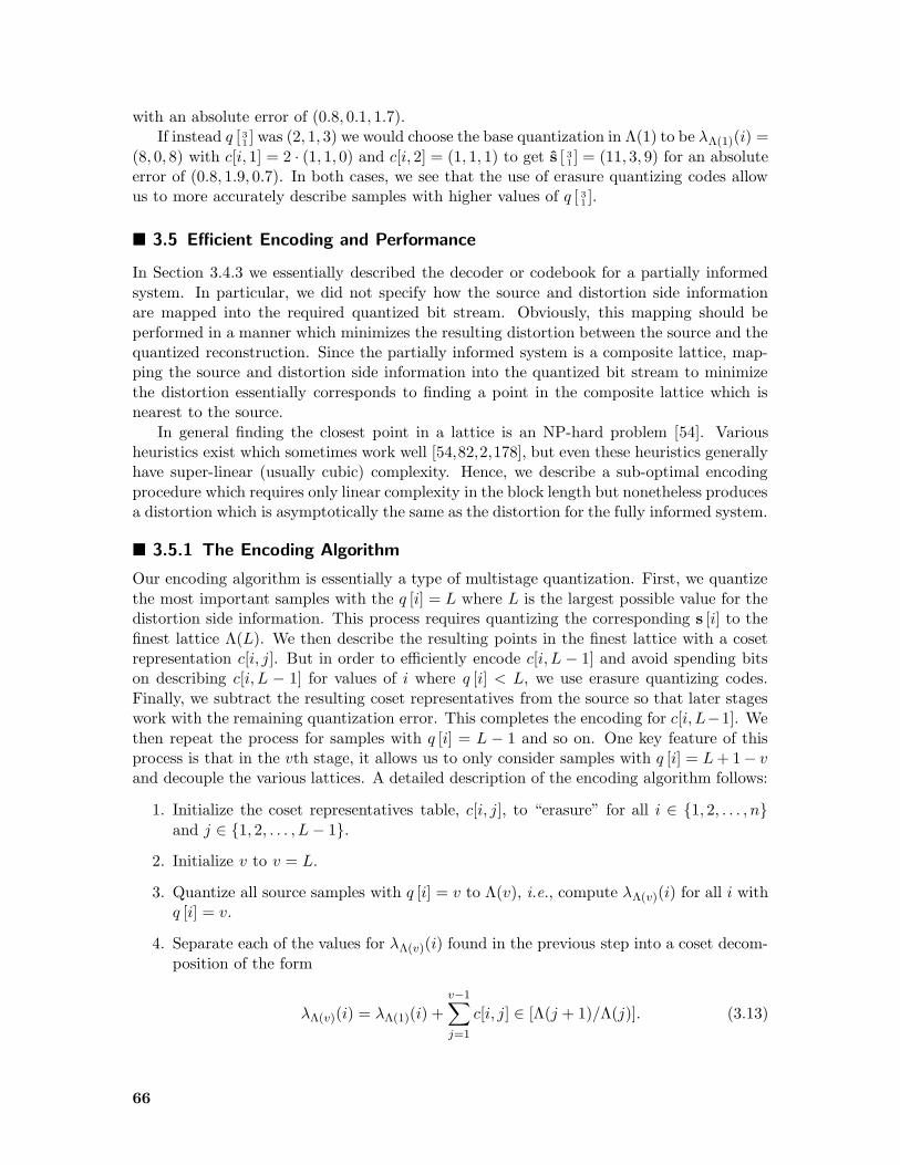
with an absolute error of (0.8, 0.1, 1.7).If instead q [ 3

1 ] was (2, 1, 3) we would choose the base quantization in Λ(1) to be λΛ(1)(i) =

(8, 0, 8) with c[i, 1] = 2 · (1, 1, 0) and c[i, 2] = (1, 1, 1) to get s [ 31 ] = (11, 3, 9) for an absolute

error of (0.8, 1.9, 0.7). In both cases, we see that the use of erasure quantizing codes allowus to more accurately describe samples with higher values of q [ 3

1 ].

� 3.5 Efficient Encoding and Performance

In Section 3.4.3 we essentially described the decoder or codebook for a partially informed

system. In particular, we did not specify how the source and distortion side informationare mapped into the required quantized bit stream. Obviously, this mapping should be

performed in a manner which minimizes the resulting distortion between the source and thequantized reconstruction. Since the partially informed system is a composite lattice, map-ping the source and distortion side information into the quantized bit stream to minimize

the distortion essentially corresponds to finding a point in the composite lattice which isnearest to the source.

In general finding the closest point in a lattice is an NP-hard problem [54]. Variousheuristics exist which sometimes work well [54,82,2,178], but even these heuristics generallyhave super-linear (usually cubic) complexity. Hence, we describe a sub-optimal encoding

procedure which requires only linear complexity in the block length but nonetheless producesa distortion which is asymptotically the same as the distortion for the fully informed system.

� 3.5.1 The Encoding Algorithm

Our encoding algorithm is essentially a type of multistage quantization. First, we quantize

the most important samples with the q [i] = L where L is the largest possible value for thedistortion side information. This process requires quantizing the corresponding s [i] to the

finest lattice Λ(L). We then describe the resulting points in the finest lattice with a cosetrepresentation c[i, j]. But in order to efficiently encode c[i, L − 1] and avoid spending bitson describing c[i, L − 1] for values of i where q [i] < L, we use erasure quantizing codes.

Finally, we subtract the resulting coset representatives from the source so that later stageswork with the remaining quantization error. This completes the encoding for c[i, L−1]. We

then repeat the process for samples with q [i] = L − 1 and so on. One key feature of thisprocess is that in the vth stage, it allows us to only consider samples with q [i] = L + 1− vand decouple the various lattices. A detailed description of the encoding algorithm follows:

1. Initialize the coset representatives table, c[i, j], to “erasure” for all i ∈ {1, 2, . . . , n}and j ∈ {1, 2, . . . , L− 1}.

2. Initialize v to v = L.

3. Quantize all source samples with q [i] = v to Λ(v), i.e., compute λΛ(v)(i) for all i withq [i] = v.

4. Separate each of the values for λΛ(v)(i) found in the previous step into a coset decom-

position of the form

λΛ(v)(i) = λΛ(1)(i) +

v−1∑

j=1

c[i, j] ∈ [Λ(j + 1)/Λ(j)]. (3.13)

66

5. Find a codeword in the (n,#[q [ n1 ] ∼ v]) near-MDS erasure quantizing code over an

alphabet of size |Λ(v)/Λ(v−1)| which exactly matches all unerased values in c[i, v−1]

for i ranging from 1 to n.

6. Subtract the resulting coset representatives from the source, i.e., for each i set s [i] to

be s [i]− c[i, v − 1].

7. Decrease v by 1.

8. If v ≥ 1 return to step 3.

9. Entropy code the description of λΛ(1)(i) for i ranging from 1 to n (e.g., using Huffmancoding, Lempel-Ziv coding, arithmetic coding, etc.).

10. The algorithm is complete and s [i] now contains the difference between the original

source and the quantized value computed by the algorithm.

� 3.5.2 An Example of Encoding

To clarify the encoding algorithm, we again return to the first example in Section 3.4.3 with

q [ 31 ] and s [ 3

1 ] as in (3.11).

In the first pass of the algorithm, we set v = 3 and quantize s [2] = 1.1 to the nearestpoint in the Z lattice to obtain λΛ(3)(2) = 1. The resulting coset representation has c[2, 2] =

1 which must be encoded by a (3,1,2) erasure quantizing code (i.e., a binary repetitioncode) to yield c[ 3

1 , 2] = 1. Thus, in step 6 of the encoding algorithm, we subtract these coset

representatives from the source to obtain

s [ 31 ]′ = (10.8, 0.1, 7.7) (3.14)

after the first stage completes.

In the second pass, we set v = 2 and quantize s [1]′ to the nearest point in the 2Z

lattice to obtain λΛ(2)(1) = 10. Note that, in the previous pass we already determined thatλΛ(3)(2) = 1 which in the coset decomposition

λΛ(3)(2) = λΛ(2)(2) + c[2, 2] (3.15)

implies that λΛ(2)(2) = 0. The resulting coset representatives for λΛ(2)(1) and λΛ(2)(2) arec[1, 1] = 2 and c[2, 1] = 0. These coset representatives must be encoded by a (3,2,1) erasurequantizing code (i.e., a binary single parity check code) to yield 2 · (1, 0, 1). Subtracting

this from the source yieldss [ 3

1 ]′′ = (8.8, 0.1, 5.7) (3.16)

at the conclusion of the second stage.

In the third pass, we set v = 1 and quantize s [3]′′ to the nearest lattice point in

the 4Z lattice to obtain λΛ(1)(3) = 4. Note that in the previous two passes we alreadyquantized the other source samples which, through the appropriate coset decomposition,

yields λΛ(1)(1) = 8 and λΛ(1)(2) = 0.

Thus after the encoding process terminates, we obtain the reconstruction in (3.12).

67

� 3.5.3 Complexity Analysis

Theorem 11. Let M(n) be the complexity of finding a codeword in step 5 of the algorithmin Section 3.5.1 and let E(n) be the complexity of entropy coding λΛ(1)(i) in step 9. Then

the complexity of this algorithm is

O (E(n) + L · (M(n) + n)) . (3.17)

Proof. The operations in steps 3, 4, and 6 each require O (n) complexity since they perform

a single operation for each source sample. The loop is performed exactly L times and socombining this with the assumed complexity for steps 5 and 9 yields (3.17).

Corollary 2. If linear-time erasure quantizing codes are used (e.g., the ones constructed in[125] along with a linear time entropy coding algorithm, then the complexity of the algorithm

in Section 3.5 is linear in the block length n.

� 3.5.4 Statistical Models and Distortion Measures

In order to the expected bit rate required using the proposed structures and the resulting

average distortion we need to introduce a statistical model for the source and distortionside information. For simplicity, we consider a memoryless source with memoryless dis-tortion side information which is independent of the source.6 Specifically, we model the

source s [n1 ] = (s [1] , s [2] , . . . , s [n]) as a sequence of either vectors or scalars taking values

in the alphabet S. The source is generated according to the independent and identically

distributed (i.i.d.) probability law

ps[n1 ](s [n

1 ]) =

n∏

i=1

ps(s [i]). (3.18)

Similarly, we model the distortion side information q [ n1 ] = (q [1] , q [2] , . . . , q [n]) as a se-

quence of scalars taking values in the finite alphabet Q. The distortion side information isindependent of the source and generated according to the i.i.d. probability law

pq[n

1 ]|s[n1 ](q [n

1 ] |s [n1 ]) =

n∏

i=1

pq(q [i]). (3.19)

Furthermore, we will focus on the special case of difference distortion measures where,for fixed q, the distortion between a source, s, and a reconstruction, s, only depends on the

difference s− s:d(s, s; q) = ρ(s− s; q) (3.20)

Admissible Lattices, Sources, and Distortion Measures

Results in the theory of lattice quantization are often developed in terms of the Voronoi

region of a basic cell of the lattice [40,63,112,64,197,58]. Specifically, for any lattice pointλ ∈ Λ(q), and the associated distortion measure, d(s, s; q), the Voronoi region of a lattice

6Extending our results to sources with memory is straightforward and simply requires replacing algo-rithms/results for losslessly compressing memoryless sources with algorithms/results for losslessly compress-ing sources with memory. In contrast, exploiting memory in the distortion side information or correlationbetween the source and distortion side information to further reduce the expected bit rate seems to requireadditional tools.

68

point V [λ ∈ Λ(q), d(s, s; q)] is the set of all points closest to that lattice point.7 For adifference distortion measure, each lattice point has the same Voronoi region.

Let us define the random variable uΛ(q),ρ(·,q) as being uniformly distributed over thisVoronoi region. Under certain mild technical conditions, the distribution of the difference

between the source and its quantized reconstruction asymptotically approaches that ofuΛ(q),ρ(·,q). Intuitively, as the density of the lattice increases, the source distribution becomesroughly constant and uniform over each Voronoi region allowing us to focus on uΛ(q),ρ(·,q).

Alternatively, a dithered quantizer can be used where a uniform random variable is addedto the source prior to quantization and subtracted out during reconstruction. The dither

makes the quantization error uniformly distributed over the Voronoi region for all resolutionsat the cost of a slight increase in rate [92,199,80].

The technical details of how the quantization error approaches a uniform distributionare somewhat involved (see [176,134] for some details). Since our main goal is to present aquantizer structure and the associated algorithm we adopt a strategy similar to [58,192,74,

72] and essentially assume that quantization error is uniform and develop the consequencesof this assumption. Specifically, we introduce the following definition:

Definition 2. A sequence of lattices, Λ(1), Λ(2), . . ., Λ(L), a source distribution ps(s) anddifference distortion a measure d(s, s; q) = ρ(s− s; q) are admissible if

1. For each q the Voronoi region of Λ(q) with respect to ρ(·; q) is well defined and bounded.

2. The quantization error in mapping s to the nearest point λ ∈ Λ(q) with respect to ρ(·; q)asymptotically approaches a uniform distribution over the Voronoi region independentof s and λ.

� 3.5.5 Rate-Distortion For Fully Informed Systems

Theorem 12. For an admissible source, nested lattice, and distortion measure, the aver-

age rate and distortion for a fully informed system asymptotically approach the followingparametric form in the high-resolution limit:

DFI∆= E

[

1

n

n∑

i=1

d(s [i] , s [i] ; q [i])

]

(3.21)

→L∑

j=1

pq(j) ·E[ρ(uΛ(q),ρ(·,q); q)|q = j] (3.22)

RFI∆=

1

nH (s [n

1 ] |q [n1 ]) (3.23)

→ h(s)− h(uΛ(1),ρ(·,1))−L∑

j=2

Pr[q ≥ j] · log |[Λ(j)/Λ(j − 1)]|. (3.24)

7For “simple” distortion measures this definition is sufficient and Voronoi regions are unique. For otherdistortion measures there may exist non-negligible regions of space which are “closest” to multiple latticepoints. In such cases, a tie-breaking rule (e.g., break ties with Euclidean distance) or some other method ofspecifying Voronoi regions may be necessary. These subtleties are beyond the scope of this work and hencewe use the upcoming Definition 2 to restrict attention to cases where these issues do not arise or can bestraightforwardly dealt with.

69

Proof. Using the linearity of expectations followed by the law of iterated expectations yields

E

[

1

n

n∑

i=1

d(s [i] , s [i] ; q [i])

]

=1

n

n∑

i=1

E [d(s [i] , s [i] ; q [i])] (3.25)

=1

n

n∑

i=1

L∑

j=1

pq(j) · E [d(s [i] , s [i] ; q [i])|q [i] = j] . (3.26)

Combining the i.i.d. nature of the probability models in (3.18) and (3.19), the special form of

the distortion measure in (3.20), and the admissibility assumption in Definition 2 establishesthat (3.26) implies (3.22).

Next, we have

1

nH (s [n

1 ] |q [n1 ]) = H (s|q) (3.27)

= I (s; s|q) (3.28)

= h(s|q)− h(s|q, s) (3.29)

= h(s|q)− h(s− s|q, s) (3.30)

→ h(s|q)− h(uΛ(q),ρ(·,q)|q) (3.31)

= h(s)− h(uΛ(q),ρ(·,q)|q) (3.32)

= h(s)−L∑

q=1

h(uΛ(q),ρ(·,q)) · pq(q) (3.33)

where (3.27) follows from the i.i.d. probability models in (3.18) and (3.19), (3.28) follows

from the fact that s [i] is a deterministic function of s [i] conditioned on q [i], (3.31) followsfrom Definition 2, and (3.32) follows from our probability model in which s and q are

statistically independent.

The random variable uΛ(q),ρ(·,q) is uniform over the Voronoi region V [Λ(q), ρ(·, q)], there-fore h(uΛ(q),ρ(·,q)) is simply the logarithm of the volume of V [Λ(q), ρ(·, q)]. Since Λ(q) ⊂Λ(q +1), however, the Voronoi region of the former is composed of |[Λ(q +1)/Λ(q)/|] copiesof the latter, i.e.,

Volume(V [Λ(q), ρ(·, q)]) = |[Λ(q + 1)/Λ(q)]| ·Volume(V [Λ(q + 1), ρ(·, q + 1)]). (3.34)

Repeatedly applying (3.34) and taking the logarithm of the resulting volume yields

h(uΛ(q),ρ(·,q)) = h(uΛ(1),ρ(·,q)) +

q∑

j=2

log |[Λ(j)/Λ(j − 1)]|. (3.35)

Furthermore, for admissible lattices and distortion measures satisfying Definition 2, thevolume of the Voronoi region does not depend on the distortion measure [41] and thus we

can replace (3.35) with

h(uΛ(q),ρ(·,q)) = h(uΛ(1),ρ(·,1)) +

q∑

j=2

log |[Λ(j)/Λ(j − 1)]|. (3.36)

70

Substituting (3.36) into (3.33) and collecting terms completes the proof.

� 3.5.6 Rate-Distortion For Partially Informed Systems

Theorem 13. For an admissible source, nested lattice, and distortion measure, the average

rate and distortion for a partially informed system asymptotically approach the rate anddistortion for a fully informed system.

Proof. For samples where q [i] = L, both the partially informed and fully informed system

quantize s [i] to the nearest point in the finest lattice Λ(L) and hence achieve the samedistortion. For q [i] = L, the fully informed system quantizes s [i] to Λ(L − 1). For thepartially informed system, s [i] is quantized to the lattice Λ(L − 1) shifted by c [i]. But

this shift does not affect the admissibility assumption in Section 2, and the quantizationerror for the shifted lattice is still uniformly distributed over the Voronoi region. Thus, the

fully informed and partially informed systems asymptotically achieve the same distortionfor samples with q [i] = L−1. This argument can be extended to all possible values of q andhence shows that the total average distortion for the fully and partially informed systems

are asymptotically equal.

We compute the contributions to the rate from the components of the partially in-

formed system listed in Section 3.4.3. As discussed in (3.10) of Section 3.4.3, the numberof bits required to encode #[q [ n

1 ] ∼ j] is at most logarithmic in n and hence asymptoticallynegligible. The rate required to encode the base lattice points λΛ(1)(i) is

h(s)− h(uΛ(1),ρ(·,1)) (3.37)

by the same arguments as in the proof of Theorem 12. All that remains is to compute therate required to encode the coset representatives as described in Section 3.4.3.

If an (n,#[q [n1 ] ∼ j], n −#[q [n

1 ] ∼ j]) MDS erasure quantizing code is used to encodethe sequence c[i, j] for each j, then the total average rate per sample required is

L∑

j=2

#[q [n1 ] ∼ j]

n· log |[Λ(j)/Λ(j − 1)]|. (3.38)

By the law of large numbers, #[q [ n1 ] ∼ j]/n converges to pq(j) and thus (3.38) converges

toL∑

j=2

pq(j) · log |[Λ(j)/Λ(j − 1)]|. (3.39)

Of course, MDS erasure quantizing codes may not exist for large n or their encoding/decodingmay be too complex. Therefore we proposed using near-MDS erasure quantizing codes withparameters (n,#[q ∼ j]+ε(n), n−#[q ∼ j]) where ε(n)→ 0 as n→∞ (i.e., the asymptotic

rate penalty for using near-MDS codes instead of MDS codes is negligible).

Summing the rate components from (3.10), (3.37), and (3.39) shows that the rate for

the partially informed system is asymptotically the same as the rate for the fully informedsystem.

71


In this chapter we have described two lattice based quantizers to use distortion side infor-mation. The first is a fully informed system where both the encoder and decoder know

the distortion side information. It is a natural application of lattice codes and entropycoding to lossy compression with distortion side information and is introduced mainly forthe purpose of comparison. The second quantizer is a partially informed system where only

the encoder knows the distortion side information. Our main result is that the partiallyinformed system can asymptotically achieve the same performance as the fully informed

system and requires only linear complexity.We feel these results are important for two main reasons. First, the distortion side

information framework provides an analytically tractable way to model a rich variety of

effects not captured by the traditional distortion measures. As mentioned previously, someexamples include perceptual distortion measures and sensor applications. Second, the con-

structions proposed in this chapter provide a low complexity way to obtain the theoreticalbenefits of using sophisticated distortion measures in a practical way.

72

Chapter 4

Iterative Quantization Using CodesOn Graphs

73

In this chapter, we study codes on graphs combined with an iterative message passingalgorithm for quantization. Specifically, we consider the binary erasure quantization (BEQ)

problem which is the dual of the binary erasure channel (BEC) coding problem. We showthat duals of capacity achieving codes for the BEC yield codes which approach the minimumpossible rate for the BEQ. In contrast, low density parity check codes cannot achieve the

minimum rate unless their density grows at least logarithmically with block length. Fur-thermore, we show that duals of efficient iterative decoding algorithms for the BEC yield

efficient encoding algorithms for the BEQ. Hence our results suggest that graphical modelsmay yield near optimal codes in source coding as well as in channel coding and that dualityplays a key role in such constructions.


Researchers have discovered that error correction codes defined on sparse graphs can be

iteratively decoded with low complexity and vanishing error probability at rates close tothe Shannon limit. Based on the close parallels between error correction and data compres-sion, we believe that similar graphical codes can approach the fundamental limits of data

compression with reasonable complexity. Unfortunately, the existing suboptimal channeldecoding algorithms for graphical codes generally fail unless the decoder input is already

near a codeword. Since this is usually not the case in source coding, either a new type ofgraph or a new suboptimal algorithm (or both) is required.

Before developing iterative quantization techniques it is worth investigating the potentialgains of such an approach over existing systems. For asymptotically high rates, when

compressing a continuous source with finite moments relative to mean square error (MSE)distortion, entropy coded scalar quantization (ECSQ) is 1.53 dB from the rate-distortion

limit [79]. For moderate rates the gap is larger: in quantizing a Gaussian source relativeto MSE distortion, ECSQ systems are 1.6–3.4 dB away from the rate-distortion limit. Forthese parameters, trellis coded quantization (TCQ) using a 256-state code with optimal

quantization has a gap of 0.5–1.4 dB [117]. For higher rates, sources with larger tails(e.g., a source with a Laplacian distribution), or sources with memory, the gaps are larger.

Thus for memoryless sources quantized at moderate rates, new codes have the potential toimprove performance by the noticeable margin of a few decibels. More generally, the codeson graphs paradigm may prove valuable in a variety of scenarios involving speech, audio,

video and other complicated sources.

To illustrate possible approaches to developing graphical codes we focus on the binaryerasure quantization (BEQ) problem which is the dual of the binary erasure channel (BEC)coding problem. First we describe the BEQ problem model in Section 4.2. Next, in Sec-

tion 4.3 we present our main result for the BEQ: duals of low density parity check codes canbe analyzed, encoded, and decoded by dualizing the corresponding techniques for the BEC.

Specifically, by dualizing capacity achieving codes for the BEC we obtain rate-distortionapproaching codes for the BEQ. Finally, we close with some concluding remarks in Sec-tion 4.4.

� 4.2 Quantization Model

Vectors and sequences are denoted with an arrow (e.g., x). Random variables or random

vectors are denoted using the sans serif font (e.g., x or x). We consider the standard(memoryless) data compression problem and represent an instance of the problem with the

74

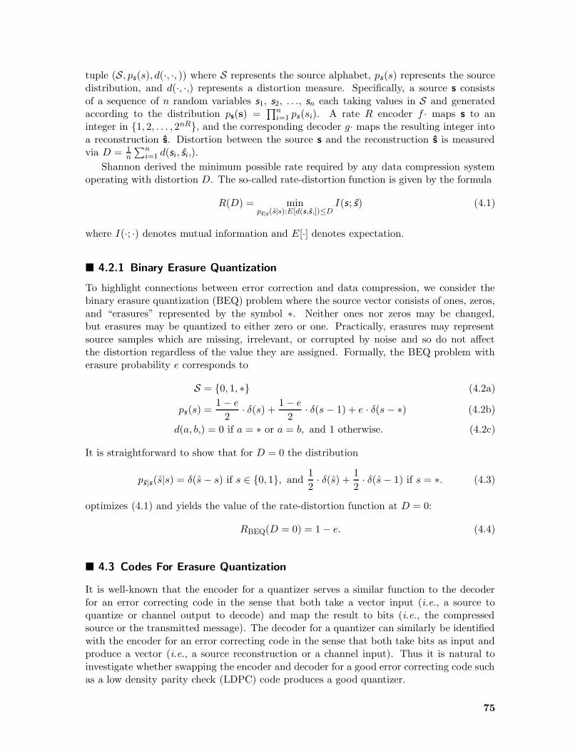
tuple (S, ps(s), d(·, ·, )) where S represents the source alphabet, ps(s) represents the sourcedistribution, and d(·, ·,) represents a distortion measure. Specifically, a source s consists

of a sequence of n random variables s1, s2, . . ., sn each taking values in S and generatedaccording to the distribution ps(s) =

∏ni=1 ps(si). A rate R encoder f · maps s to an

integer in {1, 2, . . . , 2nR}, and the corresponding decoder g· maps the resulting integer into

a reconstruction s. Distortion between the source s and the reconstruction s is measuredvia D = 1

n

∑ni=1 d(si, si,).

Shannon derived the minimum possible rate required by any data compression systemoperating with distortion D. The so-called rate-distortion function is given by the formula

R(D) = minps|s(s|s):E[d(s ,s ,])≤D

I(s; s) (4.1)

where I(·; ·) denotes mutual information and E[·] denotes expectation.

� 4.2.1 Binary Erasure Quantization

To highlight connections between error correction and data compression, we consider thebinary erasure quantization (BEQ) problem where the source vector consists of ones, zeros,

and “erasures” represented by the symbol ∗. Neither ones nor zeros may be changed,but erasures may be quantized to either zero or one. Practically, erasures may represent

source samples which are missing, irrelevant, or corrupted by noise and so do not affectthe distortion regardless of the value they are assigned. Formally, the BEQ problem witherasure probability e corresponds to

S = {0, 1, ∗} (4.2a)

ps(s) =1− e

2· δ(s) +

1− e

2· δ(s− 1) + e · δ(s− ∗) (4.2b)

d(a, b,) = 0 if a = ∗ or a = b, and 1 otherwise. (4.2c)

It is straightforward to show that for D = 0 the distribution

ps |s(s|s) = δ(s− s) if s ∈ {0, 1}, and1

2· δ(s) +

1

2· δ(s− 1) if s = ∗. (4.3)

optimizes (4.1) and yields the value of the rate-distortion function at D = 0:

RBEQ(D = 0) = 1− e. (4.4)

� 4.3 Codes For Erasure Quantization

It is well-known that the encoder for a quantizer serves a similar function to the decoder

for an error correcting code in the sense that both take a vector input (i.e., a source toquantize or channel output to decode) and map the result to bits (i.e., the compressedsource or the transmitted message). The decoder for a quantizer can similarly be identified

with the encoder for an error correcting code in the sense that both take bits as input andproduce a vector (i.e., a source reconstruction or a channel input). Thus it is natural to

investigate whether swapping the encoder and decoder for a good error correcting code suchas a low density parity check (LDPC) code produces a good quantizer.

75

� 4.3.1 LDPC Codes Are Bad Quantizers

One benefit of studying the BEQ problem is that it demonstrates why low density paritycheck (LDPC) codes are inherently unsuitable for quantization. Specifically, consider an

LDPC code like the one illustrated in Fig. 4-1 using Forney’s normal graph notation [66].If all the variables connected to a given check are not erased, then there is an even chance

that no code symbol can match the source in that position and thus the distortion willbe positive regardless of the code rate. Thus, as stated in Theorem 14 and proved inAppendix C, successful decoding is asymptotically unlikely unless the density of every parity

check matrix for the code increases logarithmically with the block length.1

Theorem 14. Let C(n) be a sequence of linear codes of length n and fixed rate R such thatthe probability that binary erasure quantization using C(n) of a random source sequence with

e · n erasures will succeed with zero distortion is bounded away from 0 as n → ∞. Thenregardless of the values of R and e, the degree of the parity-check nodes in any parity-check

graph representation of C(n) must increase at least logarithmically with n.

0 1 ** 0 *

Figure 4-1. Using an LDPC code for binary erasure quantization. The boxes with = signs are repetitionnodes: all edges connected to an = box must have the same value. The boxes with + signs are check nodes:the modulo 2 sum of the values on edges connected to a + box must be 0. The source consists of 0’s, 1’s, anderasures represented by ∗’s. Erasures may be quantized to 0 or 1 while incurring no distortion. A non-zerodistortion must be incurred for the source shown above since the left-most check cannot be satisfied.

The poor performance of LDPC codes for quantization may seem surprising in light oftheir excellent properties in channel coding, but it has long been recognized that good codes

for error correction and quantization may be different. The former is essentially a packingproblem where the goal is to place as many codewords as possible in a given space such

that the codewords are far apart and can be distinguished despite noise. The latter is acovering problem where the goal is to place as few codewords as possible in a given spacesuch that every point in space is near at least one codeword.

From any good error correcting code (respectively data compression code) it is easy toobtain another code which is almost as good at error correction (resp. data compression)

but terrible at source coding (resp. channel coding). For example, removing half thecodewords has an asymptotically negligible effect on error correction since it only decreasesthe rate by 1/n and only increases robustness. But, removing half the codewords can

dramatically hinder source coding since half the time the source may be very far from thenearest codeword. Conversely, doubling the number of codewords has an asymptotically

negligible effect on data compression since the rate only increases by 1/n while the distortion

1We may expect the density of a code to increase as it approaches the capacity or rate-distortion function,but a code whose density also increases with block length seems undesirable.

76

may decrease slightly. But doubling the number of codewords can be catastrophic for errorcorrection if it drastically reduces the distance between codewords.

� 4.3.2 Dual LDPC Codes

Many researchers have explored duality relationships between error correction and source

coding. Such work demonstrates that often a good solution for one problem can be obtainedby dualizing a good solution to the other. Continuing in this tradition, we study the

properties of dual LDPC codes for binary erasure quantization.

Formally, a length n binary linear code C is a subspace of the n dimensional vectorspace over the binary field and the dual code C⊥ is the subspace orthogonal to C. For

LDPC codes, the code C is usually specified by the parity check matrix H representing theconstraint that HxT = 0 if and only if x is a codeword. To obtain the dual code C⊥ we can

recall that the generator G⊥ of C⊥ is exactly H. If the code C is represented by a normalgraph as in Fig. 4-1, then the graph of the dual code C can be obtained by swapping + and= nodes [66]. In dualizing the code graph in this manner it may be useful to note that while

the graph of C obtained from H represents a syndrome former for C, the dualized graphrepresents an encoder for C⊥.

For example, Fig. 4-2 is obtained by dualizing the code graph in Fig. 4-1. Notice thatwhile the original code cannot quantize the source with distortion 0, the dual code can.Intuitively, the advantage of a low density encoder structure is that it provides a simple

representation of a basis which can be used to construct the desired vector. In the followingsections, we investigate the properties of dual LDPC codes for quantization with both

optimal quantization and iterative quantization.

0 1 ** *0

Figure 4-2. Using the dual of an LDPC code for binary erasure quantization. Choosing values for thevariables at the bottom produces a codeword. The values for each sample of the resulting codeword areobtained by taking the sum modulo 2 of the connected variables. In contrast to Fig. 4-1, this structure cansuccessfully match the source with no distortion if the bottom 3 variables are set to 0, 0, 1.

� 4.3.3 Optimal Quantization/Decoding and Duality

The following theorem (proved in Appendix C) demonstrates the dual relationship between

channel decoding and source quantization using optimal decoding/quantization algorithms.

Theorem 15. A channel decoder for the code C can correctly decode every received sequence

with the erasure pattern2 e if and only if a quantizer for the code C⊥ can successfully quantize

2If symbol i is erased (resp. unerased) then ei = 1 (resp. ei = 0) in our notation for erasure patterns.

77

every3 source sequence with the erasure pattern e⊥ = 1− e.

From this result we immediately obtain the following Corollary.

Corollary 3. Let C(n) be a sequence of linear codes which achieves the capacity of a bi-

nary erasure channel with erasure probability e using optimal decoding. The sequence C⊥(n)obtained by taking the duals of C(n) achieves the minimum rate for D = 0 for the BEQ with

erasure probability e⊥ = 1− e using optimal quantization.

The statement and proof of the two preceding results contain a curious duality betweenerased/known symbols in source coding and known/erased symbols in channel coding. Asimilar duality exists between a likelihood ratio, λ, and its Fourier transform Λ = 1−λ

1+λused in dualizing the sum-product algorithm [66, pp. 545–546]. Specifically, the Fouriertransform maps known/erased likelihood ratios to erased/known likelihood ratios.

� 4.3.4 Iterative Decoding/Quantization and Duality

In the following we first review the intuition behind iterative erasure decoding algorithmsand describe the particular decoding algorithm we consider in Table 4.1. Next we outlinethe intuition behind a similar approach for iterative quantization and precisely describe our

quantization algorithm in Table 4.2. Finally, we show that these algorithms are duals.

Iterative Erasure Decoding

Many iterative message-passing decoding algorithms are essentially based on the followingidea. The outgoing message on edge i of a + node is the modulo-2 sum of all incoming

messages (excluding edge i) with the proviso that if any incoming message (excluding edgei) is ∗ then the outgoing message is also ∗. For an = node, the outgoing message on edgei is ∗ only if all other incoming messages are ∗, otherwise the outgoing message is the

same as the known incoming message or messages. These message-passing rules can beinterpreted as determining the outgoing message on edge i by applying the following “sum”

and “product” formulas to all other incoming messages. 4

+ 0 1 ∗

0 0 1 ∗1 1 0 ∗∗ ∗ ∗ ∗

and

× 0 1 ∗

0 0 # 01 # 1 1∗ 0 1 ∗

(4.5)

It is well-known that such algorithms yield optimal decoding on a tree and also performwell on graphs with cycles provided appropriate scheduling and initialization rules are se-lected. Initializing all messages to ∗ and using sequential or parallel schedules are common

choices. For the purpose of proving theorems, we consider a sequential schedule in theERASURE-DECODE algorithm of Table 4.1.

3Note that some source sequences (e.g., the all zero sequence) can be successfully quantized using C⊥

regardless of e⊥. Similarly, a system which decodes ambiguous received sequences to the all zero sequencemay succeed even when many erasures occur. Thus to obtain the desired equivalence between correctdecoding and successful quantization we define correct decoding (resp. successful quantization) as beingable to deduce the transmitted codeword (resp. a codeword matching non-erased positions of the source)for every possible received sequence (resp. source) with the the erasure pattern e (resp. e⊥).

4In the product rule for erasure decoding, the symbol # denotes a contradiction which is impossible ifonly erasures and no errors occurred.

78

Table 4.1. An algorithm for iteratively decoding data with erasures.

ERASURE-DECODE(H,y)

1: while y has at least one erased sample do2: if ∃ row i of H (i.e., a check) connected to exactly one erased variable yj then3: Set yj to be the XOR of all unerased bits in the check4: else5: return FAIL6: end if7: end while8: Set x to the message variables obtained from y9: return the message variables x

Iterative Erasure Quantization

The message-passing rules in (4.5) can also be applied to the BEQ problem for graphswithout cycles provided some form of tie-breaking is used. Specifically, some variables willreceive erasure messages even after the algorithm has completed. Such variables can be

arbitrarily chosen to be either 0 or 1 and still produce a valid quantization. For examplein quantizing the source (∗, ∗, 1) with a (3,2) single parity check code, both (1, 0, 1) and

(0, 1, 1) are equally valid results and this tie can broken arbitrarily.

On a graph with cycles, however, generalizing this approach by initializing all unknownmessages to ∗ usually fails. For example, on the dual of a Gallager code or a code like the

one represented in Fig. 4-2 such an initialization rule leads to all messages being erasedat every step of the algorithm. To perform effective tie-breaking, we need to distinguishbetween variables which can be arbitrarily set to 0 or 1 and variables which have not yet

received enough information to be determined.

One way to distinguish between these cases is to denote the former as erasures with thesymbol ∗ and the latter as null messages with the symbol ∅, and initialize all messages to

∅. With this initialization, we can use the following “sum” and “product” rules: 5

+ 0 1 ∗ ∅

0 0 1 ∗ ∅

1 1 0 ∗ ∅

∗ ∗ ∗ ∗ ∗∅ ∅ ∅ ∗ ∅

and

× 0 1 ∗ ∅

0 0 # 0 01 # 1 1 1∗ 0 1 ∗ ∅

∅ 0 1 ∅ ∅

(4.6)

Specifically, the outgoing message from a + node in a graph like Fig. 4-2 is computed bycombining incoming messages from all other edges with the + rule. The outgoing message

from an = node is computed by combining incoming messages from all other edges withthe × rule. Whenever an = node has all incoming messages being ∗, the value of the node

is arbitrary. This tie can be broken by arbitrarily choosing a value of 0 or 1 provided thetie is broken consistently. Essentially, the requirement of consistent tie-breaking can beinterpreted as a constraint on the message-passing schedule: tie-breaking information for a

given tie should be propagated through the graph before other ties are broken.

In order to provide a precise algorithm for the purpose of proving theorems, we considerthe ERASURE-QUANTIZE in Table 4.2 based on applying the rules in (4.6) with a sequential

5In the product rule for erasure quantization, the symbol # denotes a contradiction. If a contradictionis generated then quantizing the given source with no distortion is impossible and the algorithm fails.

79

schedule and all tie-breaking collected into step 8.

Table 4.2. An algorithm for iteratively quantizing a source with erasures.

ERASURE-QUANTIZE(G,z)

1: while z has at least one unerased sample do2: if ∃ row i of G (i.e., a variable) connected to exactly one unerased check zj then3: Reserve message variable i to later satisfy zj and erase check zj

4: else5: return FAIL6: end if7: end while8: Arbitrarily set all unreserved message variables9: Set reserved variables to satisfy the corresponding checks starting from the last reserved variable

and working backward to the first reserved variable10: return message variables w

Iterative Algorithm Duality

Our main results regarding iterative quantization are the following three theorems stating

that ERASURE-QUANTIZE works correctly, can be analyzed in the same manner as theERASURE-DECODE algorithm, and works quickly:

Theorem 16. For any linear code with generator matrix G, ERASURE-QUANTIZE(G, z)

either fails in step 5 or else returns w such that wG matches z in all unerased positions.

Theorem 17. Consider a linear code with parity check matrix H and its dual code withgenerator matrix G⊥ = H. The algorithm ERASURE-DECODE(H,y) fails in step 5 if and

only if the algorithm ERASURE-QUANTIZE(G⊥, z) fails in step 5 where y has erasuresspecified by e and z has erasures specified by e⊥ = 1− e.

Theorem 18. The algorithm ERASURE-QUANTIZE(G, z) runs in time O (n · d) where n

is the length of z and d is the maximum degree of the graph corresponding to G.

These results (proved in Appendix C) imply that the parallel structure between erasuredecoding and erasure quantization allows us to directly apply virtually every result from

the analysis of one to the other. For example, these theorems combined with the analy-sis/design of irregular LDPC codes achieving the capacity of the binary erasure channel [139]

immediately yield the following Corollary:

Corollary 4. There exists a sequence of linear codes which can be efficiently encoded anddecoded that achieves the rate-distortion function for binary erasure quantization.


In this chapter we demonstrated how codes on sparse graphs combined with iterative decod-ing can achieve the Shannon limit for binary erasure quantization. The main contribution

of our algorithm is in recognizing the role of tie-breaking, scheduling, and initializationin iterative quantization. The key insight in our analysis is the strong dual relationship

80

between error correction and quantization for codes on graphs and their associated decod-ing/quantization algorithms (both optimal and iterative). We conjecture that the main

task in designing iterative message-passing algorithms for more general quantization prob-lems lies in designing appropriate tie-breaking, scheduling, and initialization rules for suchscenarios and exploiting similar dual relationships to channel decoding.

81

82

Chapter 5

Source Coding with Fixed Lag SideInformation

83


There is a growing consensus that understanding complex, distributed systems requiresa combination of ideas from communication and control [132]. Adding communication

constraints to traditional control problems or adding real-time constraints to communicationproblems has recently yielded interesting results [30,55,157,169,188]. We consider a relatedaspect of this interaction by exploring the possible advantages that the feedback/feedforward

in control scenarios can provide in compression. Specifically, we explore a variant of theWyner-Ziv problem [189] where causal side information about the source is available with

a fixed lag to the decoder and explore how such side information may be used.

For example, consider a remote sensor that sends its observations to a controller asillustrated in Fig. 5-1. The sensor may be a satellite or aircraft reporting the upcoming

temperature, wind speed, or other weather data to a vehicle. The sensor observationsmust be encoded via lossy compression to conserve power or bandwidth. In contrast to thestandard lossy compression scenario, however, the controller directly observes the original,

uncompressed data after some delay. The goal of the sensor observations is to provide thecontroller with information about upcoming events before they occur. Thus at first it might

not seem that observing the true, uncompressed data after they occur would be useful. Ourmain goal is to try to understand how these delayed observations of the source data (whichwe call side information) can be used. Our main result is that such information can be

quite valuable.

The following toy problem helps illustrate some relevant issues. Imagine that Alice

plays a game where she will be asked 10 Yes/No questions. Of these questions, 5 havemajor prizes while the others have minor prizes. After answering each question, she is toldthe correct answer as well as what the prize for that question is and receives the prize if

she is correct. Bob knows all the questions and the corresponding prizes beforehand andwishes to help Alice by preparing a “cheat-sheet” for her. But Bob only has room to record

5 answers. Is there a cheat-sheet encoding strategy that guarantees that Alice will alwayscorrectly answer the questions with the 5 best prizes? No such strategy exists using aclassical compression scheme. Instead, as illustrated in Section 5.3, the optimal strategy

requires an encoding which uses the fact that Alice gains information about the prize afteranswering.

In the rest of the chapter, we study the fixed lag side information problem. Since

solving the general problem seems difficult, we begin by focusing on perfect side informationwith a unit lag. This special case is the feedforward source coding problem introduced by

Pradhan [144] and is dual (in the sense of [145, 16]) to channel coding with feedback. Byusing the feedforward side information, it is possible to construct low complexity sourcePSfrag replacements

Source s [i]Sensor Controller

Delay

Compressed data m

s [i−∆]

s [i]

Figure 5-1. A sensor compresses and sends the source sequence s [1], s [2], . . ., to a controller whichreconstructs the quantized sequence s [1], s [2], . . ., in order to take some control action. After a delay or lagof ∆, the controller observes the original, uncompressed data directly.

84

coding systems which can achieve the rate-distortion bound. Specifically, [144] describeshow to adapt the Kailath-Schalkwijk scheme for the Gaussian channel with feedback [160]

to the Gaussian source squared distortion scenario with feedforward side information. Inthis chapter, we consider finite alphabet sources with arbitrary memoryless distributionsand arbitrary distortion measures. Since Ooi and Wornell’s channel coding with feedback

scheme [137] achieves the best error exponent with minimum complexity, we investigate thesource coding dual. Specifically, we show that the source coding dual of the Ooi–Wornell

scheme achieves the rate-distortion bound with linear complexity.

We begin by describing the problem in Section 5.2. Next we present a simple example ofhow feedforward side information can be useful in the binary erasure quantization problem

in Section 5.3. In Section 5.4, we consider the more complicated example of quantizing abinary source with respect to Hamming distortion. We present our source coding algorithmfor general sources in Section 5.5 and show that it achieves the rate-distortion function with

low complexity. We close with some concluding remarks in Section 5.6.

� 5.2 Problem Description

Random variables are denoted using the sans serif font (e.g., x) with deterministic valuesusing serif fonts (e.g., x). We represent the ith element of a sequence as x [i] and denote a

subsequence including elements from i to j as x [ ji ].

We consider (memoryless) source coding with fixed lag side information and represent aninstance of the problem with the tuple (S,W, ps,w , d(·, ·, , )∆) where S andW represent the

source and side information alphabets, ps,w (s,w) represents the source and side informationjoint distribution, d(·, ·,) represents the distortion measure, and ∆ represents the delay or

lag. Specifically, the source and side information each consist of a sequence of n randomvariables s [n

1 ] and w [n1 ] taking values in S and W generated according to the distribution

ps[ n

1 ],w[n1 ](s [n

1 ]) =∏n

i=1 ps,w (s [i] , w [i]).

A rate R encoder, f(·), maps s [n1 ] to a bit sequence represented as an integer m ∈

{1, 2, . . . , 2nR}. The corresponding decoder f−1(·) works as follows. At time i, the decodertakes as input m as well as the side information samples, w [ i−∆

1 ], and produces the ith

reconstruction s [i]. A distortion of d(s [i] , s [i] ,) is then incurred for the ith sample whered(·, ·,) is a mapping from S × S to the interval [0, dmax].

The basic problem can be specialized to the original (non-causal) Wyner-Ziv problem

[189], by allowing a negative delay ∆ = −∞. Similarly, setting ∆ = 0 yields a causal versionof the Wyner-Ziv problem. Finally, letting the side information be exactly the same as thesource with a positive delay yields the feedforward source coding problem studied in [144].

For all these cases, the goal is to understand the fundamental rate-distortion-complexityperformance. To show that the benefits of fixed lag side information are worth investigating,

we focus on the feedforward case where w = s with unit delay ∆ = 1 throughout the restof this chapter.

For memoryless sources, the information feedforward rate-distortion function, R(I)f (D),

is defined to be the same as Shannon’s classical rate-distortion function:

R(I)f (D) = inf

ps|s :E[d(s ,s ,])≤DI (s; s). (5.1)

The operational feedforward rate-distortion function, Rf(D), is the minimum rate required

85

such that there exists a sequence of encoders and decoders with average distortion,

1

n

n∑

i=1

d(s [i] , s [i]),

asymptotically approaching D. As observed in [144] and shown in the appendix, the infor-mation and operational feedforward rate-distortion functions are the same. Thus feedfor-

ward does not reduce the rate required, but as we argue in the rest of this chapter, it allowsus to approach the rate-distortion function with low complexity.

� 5.3 Example: Binary Source & Erasure Distortion

The simplest example in channel coding with feedback is the erasure channel and in this casethe algorithm in Fig. 5-2 achieves capacity. At time 1 the encoder puts message bit m [1]

into the channel. If it is received correctly, the transmitter then transmits m [2], otherwisem [1] is repeated until it is successfully received. The same process is used for m [2], m [3],

etc. For example, to send the message 0101 though a channel where samples 2, 3, 6, and7 are erased, the transmitter would send 01110111 and the receiver would see 0 ∗ ∗10 ∗ ∗1.In general, if there are n message bits, m [1], m [2], . . ., m [n], and e erasures, then exactly

n+e channel uses are required. This yields a transmission rate of n/(n+e) which is exactlythe channel capacity.

PSfrag replacements increase i increase i

StartStart

i = 1i = 1 Yes

Yes

No

No

Send m [i]

through

channel

z = next

channel

samplez erased?

m [i] = z

channel

erased?

Figure 5-2. Encoder (left) for transmitting a message m = m1, m2, . . . across an erasure channel withfeedback and decoder (right) for producing an estimate of the transmitted message m.

The dual to the binary erasure channel (BEC) is the binary erasure quantization prob-lem (BEQ). In the BEQ, each source sample can be either 0, 1, or * where * represents

“don’t care”. The distortion measure is such that 0 and 1 cannot be changed but * can bequantized to either 0 or 1 with no distortion. The BEQ models the game introduced in the

introduction.1 To develop a source coding with feedforward algorithm for the BEQ, we candualize the channel coding with feedback algorithm for the BEC as illustrated in Fig. 5-3.

1Yes/No answers for questions with major prizes map to 1/0 values for the source while questions with mi-nor prizes map to a value of * for the source. The distortion measure represents the restriction that questionswith major prizes must be answered correctly while the answers for the other questions are irrelevant.

86

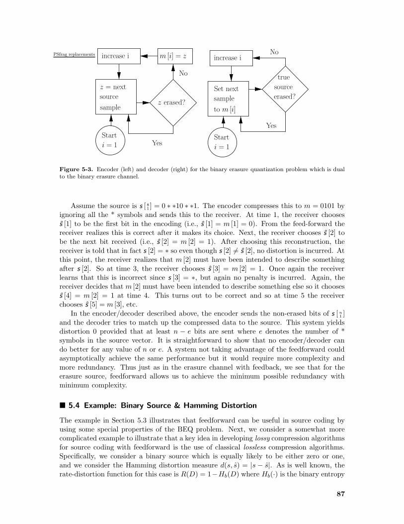
PSfrag replacementsincrease iincrease i

StartStart

i = 1i = 1

Yes

Yes

No

No

Set next

sample

to m [i]

z = next

source

samplez erased?

m [i] = z

true

source

erased?

Figure 5-3. Encoder (left) and decoder (right) for the binary erasure quantization problem which is dualto the binary erasure channel.

Assume the source is s [ 81 ] = 0 ∗ ∗10 ∗ ∗1. The encoder compresses this to m = 0101 by

ignoring all the * symbols and sends this to the receiver. At time 1, the receiver chooses

s [1] to be the first bit in the encoding (i.e., s [1] = m [1] = 0). From the feed-forward thereceiver realizes this is correct after it makes its choice. Next, the receiver chooses s [2] tobe the next bit received (i.e., s [2] = m [2] = 1). After choosing this reconstruction, the

receiver is told that in fact s [2] = ∗ so even though s [2] 6= s [2], no distortion is incurred. Atthis point, the receiver realizes that m [2] must have been intended to describe something

after s [2]. So at time 3, the receiver chooses s [3] = m [2] = 1. Once again the receiverlearns that this is incorrect since s [3] = ∗, but again no penalty is incurred. Again, thereceiver decides that m [2] must have been intended to describe something else so it chooses

s [4] = m [2] = 1 at time 4. This turns out to be correct and so at time 5 the receiverchooses s [5] = m [3], etc.

In the encoder/decoder described above, the encoder sends the non-erased bits of s [ n1 ]

and the decoder tries to match up the compressed data to the source. This system yieldsdistortion 0 provided that at least n − e bits are sent where e denotes the number of *symbols in the source vector. It is straightforward to show that no encoder/decoder can

do better for any value of n or e. A system not taking advantage of the feedforward couldasymptotically achieve the same performance but it would require more complexity and

more redundancy. Thus just as in the erasure channel with feedback, we see that for theerasure source, feedforward allows us to achieve the minimum possible redundancy withminimum complexity.

� 5.4 Example: Binary Source & Hamming Distortion

The example in Section 5.3 illustrates that feedforward can be useful in source coding byusing some special properties of the BEQ problem. Next, we consider a somewhat morecomplicated example to illustrate that a key idea in developing lossy compression algorithms

for source coding with feedforward is the use of classical lossless compression algorithms.Specifically, we consider a binary source which is equally likely to be either zero or one,

and we consider the Hamming distortion measure d(s, s) = |s − s|. As is well known, therate-distortion function for this case is R(D) = 1−Hb(D) where Hb(·) is the binary entropy

87

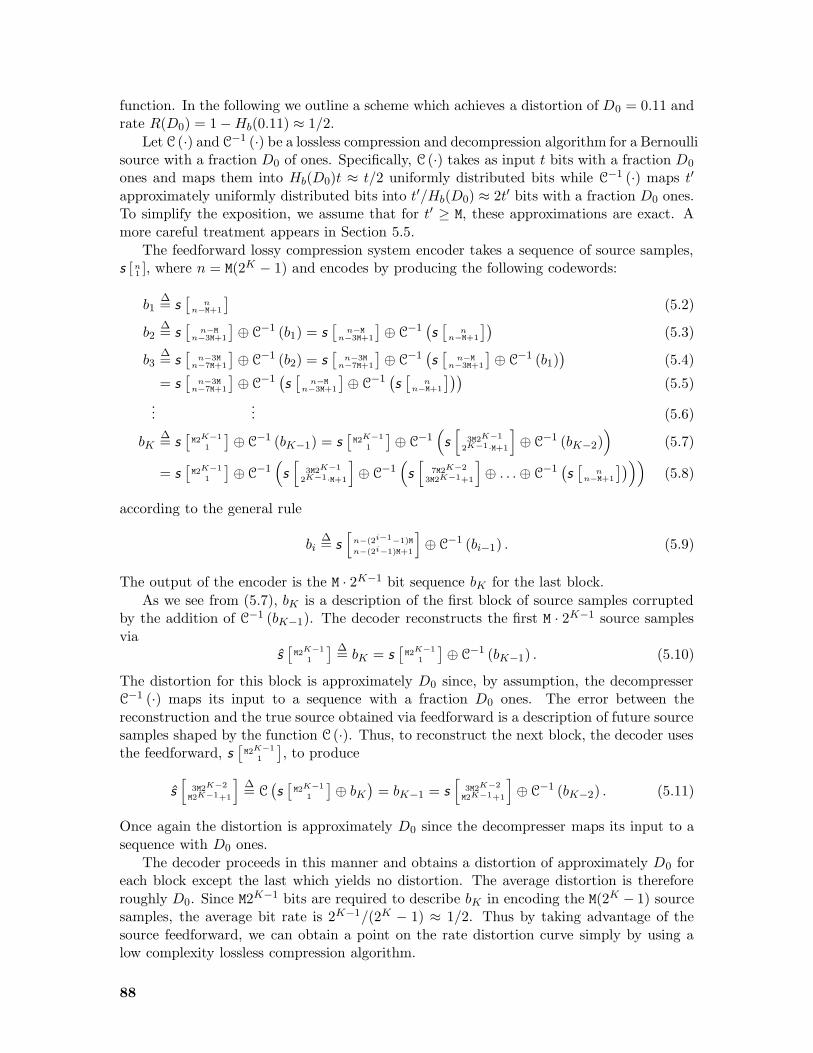
function. In the following we outline a scheme which achieves a distortion of D0 = 0.11 andrate R(D0) = 1−Hb(0.11) ≈ 1/2.

Let C (·) and C−1 (·) be a lossless compression and decompression algorithm for a Bernoulli

source with a fraction D0 of ones. Specifically, C (·) takes as input t bits with a fraction D0

ones and maps them into Hb(D0)t ≈ t/2 uniformly distributed bits while C−1 (·) maps t′

approximately uniformly distributed bits into t′/Hb(D0) ≈ 2t′ bits with a fraction D0 ones.To simplify the exposition, we assume that for t′ ≥ M, these approximations are exact. A

more careful treatment appears in Section 5.5.

The feedforward lossy compression system encoder takes a sequence of source samples,s [n

1 ], where n = M(2K − 1) and encodes by producing the following codewords:

b1∆= s

[n

n−M+1

](5.2)

b2∆= s

[n−M

n−3M+1

]⊕ C

−1 (b1) = s[

n−Mn−3M+1

]⊕ C

−1(s[

nn−M+1

])(5.3)

b3∆= s

[n−3M

n−7M+1

]⊕ C

−1 (b2) = s[

n−3Mn−7M+1

]⊕ C

−1(s[

n−Mn−3M+1

]⊕ C

−1 (b1))

(5.4)

= s[

n−3Mn−7M+1

]⊕ C

−1(s[

n−Mn−3M+1

]⊕ C

−1(s[

nn−M+1

]))(5.5)

...... (5.6)

bK∆= s

[M2K−1

1

]⊕ C

−1 (bK−1) = s[M2K−1

1

]⊕ C

−1(

s[

3M2K−1

2K−1·M+1

]

⊕ C−1 (bK−2)

)

(5.7)

= s[M2K−1

1

]⊕ C

−1(

s[

3M2K−1

2K−1·M+1

]

⊕ C−1(

s[

7M2K−2

3M2K−1+1

]

⊕ . . .⊕ C−1(s[

nn−M+1

])))

(5.8)

according to the general rule

bi∆= s

[n−(2i−1−1)M

n−(2i−1)M+1

]

⊕ C−1 (bi−1) . (5.9)

The output of the encoder is the M · 2K−1 bit sequence bK for the last block.

As we see from (5.7), bK is a description of the first block of source samples corruptedby the addition of C−1 (bK−1). The decoder reconstructs the first M · 2K−1 source samples

vias[M2K−1

1

] ∆= bK = s

[M2K−1

1

]⊕ C

−1 (bK−1) . (5.10)

The distortion for this block is approximately D0 since, by assumption, the decompresserC−1 (·) maps its input to a sequence with a fraction D0 ones. The error between the

reconstruction and the true source obtained via feedforward is a description of future sourcesamples shaped by the function C (·). Thus, to reconstruct the next block, the decoder usesthe feedforward, s

[M2K−1

1

], to produce

s[

3M2K−2

M2K−1+1

]∆= C

(s[M2K−1

1

]⊕ bK

)= bK−1 = s

[3M2K−2

M2K−1+1

]

⊕ C−1 (bK−2) . (5.11)

Once again the distortion is approximately D0 since the decompresser maps its input to a

sequence with D0 ones.

The decoder proceeds in this manner and obtains a distortion of approximately D0 foreach block except the last which yields no distortion. The average distortion is therefore

roughly D0. Since M2K−1 bits are required to describe bK in encoding the M(2K − 1) sourcesamples, the average bit rate is 2K−1/(2K − 1) ≈ 1/2. Thus by taking advantage of the

source feedforward, we can obtain a point on the rate distortion curve simply by using alow complexity lossless compression algorithm.

88

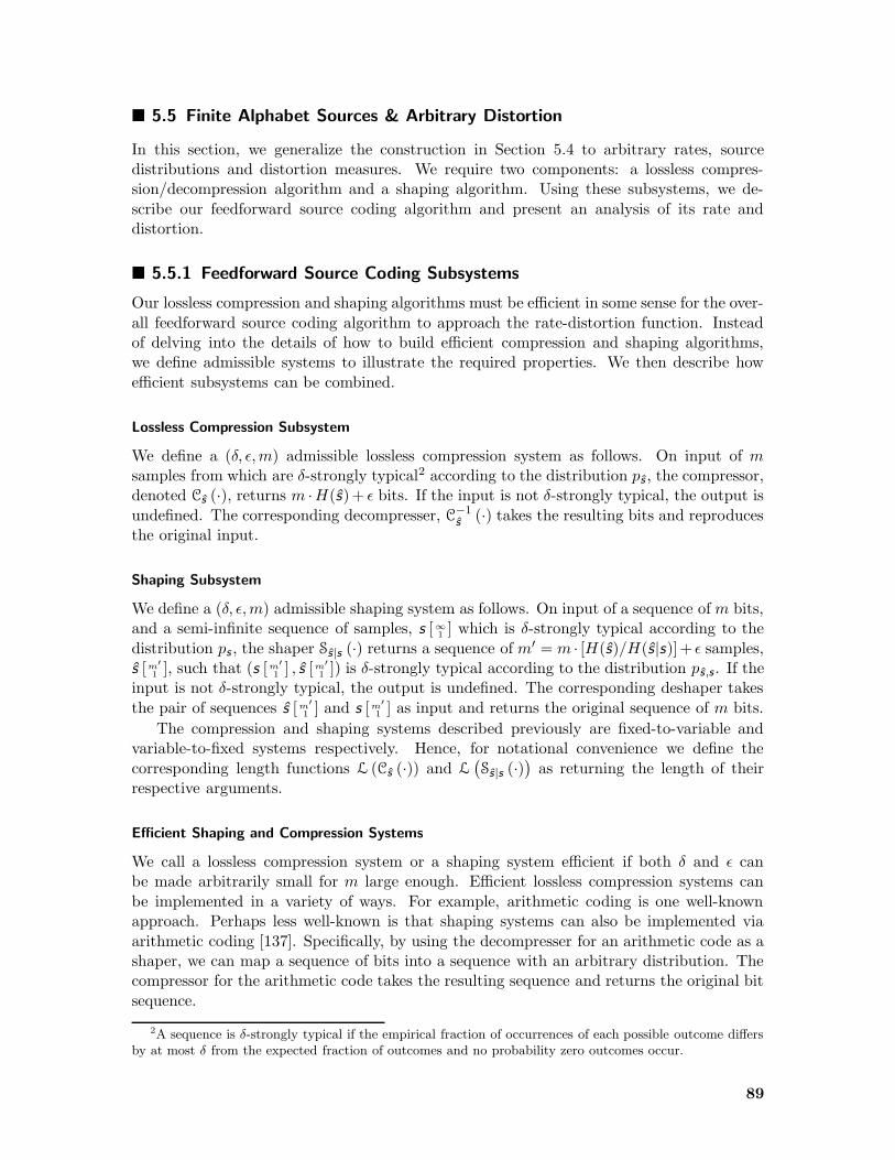
� 5.5 Finite Alphabet Sources & Arbitrary Distortion

In this section, we generalize the construction in Section 5.4 to arbitrary rates, sourcedistributions and distortion measures. We require two components: a lossless compres-sion/decompression algorithm and a shaping algorithm. Using these subsystems, we de-

scribe our feedforward source coding algorithm and present an analysis of its rate anddistortion.

� 5.5.1 Feedforward Source Coding Subsystems

Our lossless compression and shaping algorithms must be efficient in some sense for the over-

all feedforward source coding algorithm to approach the rate-distortion function. Insteadof delving into the details of how to build efficient compression and shaping algorithms,we define admissible systems to illustrate the required properties. We then describe how

efficient subsystems can be combined.

Lossless Compression Subsystem

We define a (δ, ε,m) admissible lossless compression system as follows. On input of msamples from which are δ-strongly typical2 according to the distribution ps , the compressor,denoted Cs (·), returns m ·H (s)+ ε bits. If the input is not δ-strongly typical, the output is

undefined. The corresponding decompresser, C−1s (·) takes the resulting bits and reproduces

the original input.

Shaping Subsystem

We define a (δ, ε,m) admissible shaping system as follows. On input of a sequence of m bits,and a semi-infinite sequence of samples, s [∞1 ] which is δ-strongly typical according to the

distribution ps , the shaper Ss |s (·) returns a sequence of m′ = m · [H (s)/H (s|s)]+ ε samples,s [m′

1 ], such that (s [m′

1 ] , s [m′

1 ]) is δ-strongly typical according to the distribution ps ,s . If theinput is not δ-strongly typical, the output is undefined. The corresponding deshaper takes

the pair of sequences s [m′

1 ] and s [m′

1 ] as input and returns the original sequence of m bits.

The compression and shaping systems described previously are fixed-to-variable andvariable-to-fixed systems respectively. Hence, for notational convenience we define the

corresponding length functions L (Cs (·)) and L(Ss |s (·)

)as returning the length of their

respective arguments.

Efficient Shaping and Compression Systems

We call a lossless compression system or a shaping system efficient if both δ and ε canbe made arbitrarily small for m large enough. Efficient lossless compression systems can

be implemented in a variety of ways. For example, arithmetic coding is one well-knownapproach. Perhaps less well-known is that shaping systems can also be implemented via

arithmetic coding [137]. Specifically, by using the decompresser for an arithmetic code as ashaper, we can map a sequence of bits into a sequence with an arbitrary distribution. Thecompressor for the arithmetic code takes the resulting sequence and returns the original bit

sequence.

2A sequence is δ-strongly typical if the empirical fraction of occurrences of each possible outcome differsby at most δ from the expected fraction of outcomes and no probability zero outcomes occur.

89

� 5.5.2 Feedforward Encoder and Decoder

Since the encoder for our feedforward lossy compression system is based on a variable-to-fixed shaper and a fixed-to-variable compressor, it is a variable-to-variable system. In

practice, one could use buffering, padding, or other techniques to account for this whenencoding a fixed length source or when required to produce a fixed length encoding. We

do not address this issue further here. Instead, we assume that there is a nominal sourceblock size parameter, N, and buffering, padding, look-ahead, etc. is used to ensure that thesystem encodes N source samples (or possibly slightly more or less). Also, we assume that

there is a minimum block size parameter, M, which may be chosen to achieve an efficientshaping or lossless compression subsystem.

Once N and M are fixed, the feedforward encoder takes as input a stream of inputss [∞1 ] and encodes it as described in Table 5.1. The feedforward decoder takes as input theresulting bit string, b, and decodes it as described in Table 5.2. Section 5.4 describes an

example of the encoding and decoding algorithm with a shaper (denoted C−1 (·)) mapping

uniform bits to Bernoulli(0.11) bits. This example does not require a compressor because

the ps distribution is incompressible.

Table 5.1. The Feedforward Encoder.

1: Initialize T = 1, L = M, and reverse the input so that in the following s [ n

1] = s [ 1

n].

2: Take the block of source samples s [ T+L

T] and generate a “noisy version” s [ T+L

T] (e.g., by

generating each s [i] from the corresponding s [i] according to ps|s).3: while L + T < N do4: Compress s [ T+L

T] to obtain the bit sequence b = Cs (s [ T+L

T]).

5: T ← T + L + 16: L← L

(Ss |s (b, s [∞

T])).

7: s [T+L

T]← Ss|s (b, s [∞

T])

8: end while9: return Cs (s [T+L

T])

Table 5.2. The Feedforward Decoder.

1: Initialize T to the length of the sequence encoded in b.2: while T > 1 do3: L← L

(C−1s (b)

)

4: T ← T − L + 15: s [T+L

T]← C

−1s (b)

6: Get s [ T+L

T] via the feedforward information

7: b← S−1s|s (s [T +L

T] , s [ T+L

T])

8: end while9: return the reversed version of s [n

1]

90

� 5.5.3 Rate-Distortion Analysis

Theorem 19. By using efficient lossless compression and shaping subsystems, the dis-tortion in encoding an i.i.d. sequence generated according to ps can be made to approach

E[d(s, s, ]) as closely as desired.

Proof. First we note that by assumption, we can choose M large enough so that the proba-bility of the source sequence being non-typical can be made negligible. For a typical source

sequence, we can focus on how the encoder maps s [i] to s [i] since the decoder simply maps abit sequence to the s [i] sequence chosen by the encoder. The encoder maps blocks of source

samples, s [T+LT ], to blocks of quantized samples, s [ T+L

T ], by using an admissible shapingalgorithm. As described in Section 5.5.1, the shaper produces a δ-strongly typical sequence.Thus the total expected distortion is at most

E[d(s, s, ]) + dmax · δ + dmax · Pr[s [n1 ] not typical] (5.12)

where the first two terms are the distortion for a typical sequence produced by the shaperand the last term is the contribution from a non-typical source sequence.

Theorem 20. By using efficient lossless compression and shaping subsystems, the rate inencoding an i.i.d. sequence generated according to ps can be made to approach I(s; s) as

closely as desired.

Proof. Imagine that the parameter N is chosen so that K passes of the loop in the encodingalgorithm are executed. Also, let Lj denote the value of L in line 3 of the encoder in the

jth pass. We know L1 = M by construction. By definition of an admissible shaping systemin Section 5.5.1 and line 6 of the encoder we have that Lj+1 ≥ Lj · [H (s)/H (s|s)]. Using

this relation and assuming that each block of length Lj is typical, we can compute the totalnumber of samples encoded via

n =

K∑

j=1

Lj ≥K−1∑

j=0

M ·[

H (s)

H (s|s)

]j

= M · [H (s)/H (s|s)]K − 1

H (s)/H (s|s)− 1. (5.13)

The bit rate required to encode these samples is

R = LK ·H (s) + ε ≤ M ·H (s) · [H (s)/H (s|s)]K−1 + ε ·K · [H (s)/H (s|s)]K . (5.14)

This follows by the assumption that the admissible lossless compression system in Sec-

tion 5.5.1 requires m ·H (s) + ε bits to encode a block of m typical samples.Therefore the number of bits per sample when the source blocks are typical is obtained

by dividing (5.14) by (5.13) to obtain

R/n ≤{

M ·H (s) ·[

H (s)

H (s|s)

]K−1

+ ε ·K ·[

H (s)

H (s|s)

]K}/{

M · [H (s)/H (s|s)]K − 1

H (s)/H (s|s)− 1

}

(5.15)

=

{

H (s)

[

1− H (s|s)H (s)

]

+εK

M

[H (s)

H (s|s) − 1

]}/{

1−[

H (s)

H (s|s)

]−K}

(5.16)

= I (s; s) ·{

1 +εK

MH (s|s)

}/{

1−[

H (s)

H (s|s)

]−K}

. (5.17)

91

An extra term must also be added to account for the possibility that the source is atypical.By assumption we can choose N so that K is large enough to make the second term in

braces negligible, and then we can choose M so that the probability of any source blockbeing typical is negligible. Also, by making M large enough we can make the first term incurly braces negligible. Thus the bit rate can be made as close to I (s; s) as desired.

Combining the previous theorems indicates that we can approach the feedforward rate-distortion function with only the complexity required for lossless compression and shaping

systems.

Corollary 5. When linear complexity admissible lossless compression and shaping systemsare used, the resulting feedforward rate-distortion function can be approached arbitrarilyclosely with linear complexity.

In particular, we can use the lossless compression and shaping systems described in [137]

which are based on arithmetic coding and the dual of arithmetic coding respectively.


In this chapter we describe a lossy compression algorithm to encode a finite-alphabet source

in the presence of feedforward information. In particular, we show that although memorylessfeedforward does not change the rate-distortion function, it allows us to construct a lowcomplexity lossy compression system which approaches the rate-distortion function. In

practice, the particular scheme described here may require modifications and other methodsof using feedforward information or similar knowledge may be more appropriate. Our main

goal therefore is not necessarily to advocate a particular scheme but to show that whencompression, observation, and control interact, additional resources such as feedforwardmay provide advantages not available in the classic compression framework. One interesting

possibility for future work includes studying the general problem in Section 5.2 when thefixed lag side information, w , is not exactly the same as the source. Similarly, investigating

the effects of memory in the source and different values for the delay, ∆, would also bevaluable.

92

Part II

Delay Constraints

93

94

Chapter 6

System Model

95

In this section we outline the system model we plan to study in this part of the thesis.Our main goal is to introduce a general model motivated by delay sensitive applications,

discuss the key features of this model and note its relationship to previous work. Laterchapters further specialize the model when necessary.

As demonstrated by Shannon [162], arbitrarily low error probability can be achieved

in transmitting messages across memoryless, noisy channels provided that the transmissionrate is below the channel capacity and long channel codes are used. Similarly, a sourcecan be encoded with minimum distortion provided long source codes are used in quantizing

the source. However, when the channel suffers occasional impairments due to signal fading,shadowing, mobility, congestion, interference, etc., and delay constraints prohibit averaging

over these impairments, Shannon capacity may no longer be a relevant measure.

Specifically, achieving the (ergodic) Shannon capacity of a channel requires coding overa long enough block that the transmission encounters each channel state in proportion to

its probability. When latency constraints limit the length of the transmission, arbitrarilylow error probability may be unattainable at rates approaching the Shannon capacity. Sim-ilarly, when the source statistics vary due to motion, sudden activity, or other correlations,

achieving optimal distortion may be impossible due to latency constraints. In the sequel,we present these issues in the channel coding framework with the understanding that our

models can be translated to the source coding problem in a straight-forward manner.

� 6.0.1 Notation

In this part of the thesis we continue our notational conventions from the previous part.

Vectors and sequences are denoted in bold (e.g., x) with the ith element denoted as x [i].Random variables are denoted using the sans serif font (e.g., x) while random vectors and

sequences are denoted with bold sans serif (e.g., x). Subsequences are denoted by stacking(e.g., x [ j

i ] denotes the subsequence x [i], x [i + 1], . . ., x [j]).

� 6.1 Channel Models

A general (memoryless) channel model which captures these effects can be constructed by

letting the channel output vector, y, depend on the channel input vector, x, with a differentprobability law for each sample

py|x(y|x) =∏

i

py |x ;θ(y [i] |x [i] ; θ [i]). (6.1)

where θ [0], θ [1], . . . denote channel states (e.g., modeling the level of fading or amount ofinterference).

To model packet based systems as well as systems where the channel state changes

relatively slowly, researchers often use piece-wise constant or block-interference channelmodels [126] [23] [93] [141]. In such channels the inputs and outputs are grouped intoblocks x [0], x [1], . . ., x [T] and y [0], y [1], . . ., y [T] where each block consists of nc samples:

x [i] = x0[i], x1[i], . . ., xnc−1[i] and y [i] = y0[i], y1[i], . . ., ync−1[i]. The channel law is constantfor each block:

T∏

i=0

py[i]|x[i];θ[i](y [i] |x [i] ; θ [i]) =

T∏

i=0

nc∏

j=1

py |x ;θ(yj [i]|xj [i]; θ [i])

96

where the block size, nc, typically depends on problem details such as the coherence time inwireless communication or the Maximum Transmit Unit (MTU) in wired networks. When

coding is allowed only over a single block (i.e., T = 0), this (non-ergodic) channel is some-times referred to as the compound channel [50] or a class of channels [25], [187].

Ideally, T should be large enough that the receiver can average over the channel variationsand obtain arbitrarily low probability of error provided that the transmission rate is below

the ergodic capacity. However, due to delay constraints, T is often constrained to be finiteand reliably transmitting rates approaching the ergodic capacity is not possible. In this

case, previous researchers have characterized performance using measures such as outagecapacity [141] [23] or delay-limited capacity [81].

While such work highlights some key issues in dealing with time-varying channel uncer-tainty, in order to focus on real-time applications where delay and causality are important

constraints, we consider a sequential model which requires block Markov coding [45]. Specif-ically, we consider the model where the transmitter has a sequence of messages, s [i], to sendover the channel. At each time step, the transmitter chooses the channel input x [i] as a

function of s [i], s [i− 1], . . . and the receiver obtains the corresponding channel output y [i].The receiver’s goal is to reliably estimate s [i] within a given delay constraint (to be defined

shortly).

There are two key differences between the sequential model and previous models. First,instead of sending a fixed length message, s, known before transmission begins, the encodermust send a stream of messages, s [i], revealed causally. Second, instead of only measuring

whether the entire message (or even a piece of the message) can be decoded eventually,we are interested in the decoding delay. As we shall argue, the sequential model is suited

to delay sensitive applications such as video or audio streaming, two-way communications,remote control, and many others. Furthermore, we shall demonstrate that it leads to a richset of new algorithms for real-time communication.

� 6.2 Notions Of Delay

Many formulations of communication problems with delay exist. Before we choose a model

and explore the resulting conclusions, it is useful to consider what issues we are trying tounderstand with a given definition of delay. For example, error exponents are one commonnotion of delay (i.e., a block notion). The analysis of error exponents essentially asks “How

large a block is required to achieve the performance promised by random coding argumentsand the law of large numbers?” The theory of error exponents answering this question is

useful in deciding how large a block (and correspondingly how much latency) to use in ablock code. But we are interested in a different question: “How do we design codes whichcan be quickly decoded despite dynamic channel fluctuations?”. Therefore, after discussing

various notions of delay we introduce the idea of “packet delay” we use in the rest of thethesis.

� 6.2.1 Block-Delay

Consider transmitting a message which consists of one long file. For such messages, a

natural performance measure is the block-delay: the length of time between when theencoder starts transmitting and when the receiver decodes the entire message. Generally,

block-delay is an appropriate performance measure for monolithic messages where no pieceof the message is useful without the whole. Block-delay seems to be one of the earliest

97

measure of delay and is connected to the traditional analysis of error exponents (for standardchannels) as well as outage-capacity or delay-limited capacity (for compound channels).

Recently, codes designed to minimize the block-delay in transmitting large files have beenreported [115,31,163,59,53].

However, certain information sources possess a natural ordering of distinct segments(e.g., video, audio, sequential sensor readings, or statements in two-way conversations).

Decoding earlier portions of a message of this kind before the entire message is received isnot only valuable but sometimes essential. For such systems, other measures of delay aredesirable.

� 6.2.2 Symbol-Delay

Perhaps the most basic way to measure decoding delay in a sequential model is via the

symbol-delay i.e., the number of time units between when s [i] is sent and it is decoded(neglecting any propagation delay). Essentially, this corresponds to considering packets oflength nc = 1. For example, if a convolutional encoder with constraint length L is used with

a Viterbi decoder, then it is well-known that a decoding delay of 5L causes a negligible lossin performance [151]. The symbol-delay (or in this case the bit-delay) for a system designed

to make decisions according to this criteria would be simply 5L as illustrated in Fig. 6-1 forthe case of L = 4.

Source Sequence: s [0] s [1] . . . s [20] s [21] s [22] s [23] s [24] s [25]Encoded Sequence: x [0] x [1] . . . x [20] x [21] x [22] x [23] x [24] x [25]

Channel Output: y [0] y [1] . . . y [20] y [21] y [22] y [23] y [24] y [25]Decoder Output: . . . . . . . . . s [0] s [1] s [2] s [3] s [4] s [5]

Figure 6-1. Illustration of a system with a bit-delay of 20.

However, if long delays are undesirable, some symbols may be decoded earlier and some

later resulting in a different symbol-delay for each message element. In such cases, statisticalcharacteristics of the symbol-delay (e.g., moments of the symbol-delay, the symbol-delayhistogram, or the decay rate of the histogram) may be appropriate.

� 6.2.3 Packet-Delay

Symbol-delay may seem like the most complete delay characterization (though potentially

intractable to analyze). For example, symbol-delay subsumes block-delay in the sense thatif all the symbols are presented to the encoder simultaneously, then the maximum symbol-delay is exactly the block-delay. However, the concept of symbol-delay fails to capture a

key facet of many practical systems: packetization.

Consider a music or video streaming system or a video-conferencing system. In suchsystems the encoder receives a sequence of audio or video samples to quantize from themicrophone or camera. Usually, however, these source samples are not quantized as they

are received but blocked into a packet and encoded together in order to apply powerfulsource coding techniques such as vector quantization, LPC coding, wavelet transforms, etc.

Furthermore, at the physical layer, information is usually collected into packets due to thebenefits of packet switched communications.

98

Thus measuring the time interval between when a certain audio or video sample enteredthe encoder and was reconstructed at the receiver is not especially meaningful. Instead, it is

more useful to consider the time interval between when a source packet entered the encoderand when it was reconstructed by the decoder. Consequently, for packet based systems weintroduce the following notion of packet-delay.

Let the encoder input be a sequence of message packets s [i] where each message packetis composed of ns samples s0[i], s1[i], . . ., sns−1[i]. The encoder transforms the input packet

stream into a sequence of channel input packets of length nc, x [i] = x0[i], x1[i], . . . , xnc−1[i],which are transmitted to the receiver. A decoder takes the resulting channel output packets,y [i], and produces an estimate of the original message s [i]. The packet-delay is the number

of time units between when s [i] is sent and s [i] is decoded. Essentially, one can think ofcoding in the packet-delay setting as using a type of convolutional code where the basic unit

is a “super-symbol” instead of a bit and each super-symbol corresponds to a single packet.In the sequel, we will focus on packet-delay since it most closely models practical systems

of interest. For many voice, video and audio applications and many physical layer designs,

packet sizes are reasonably large. Consequently, we study limiting performance as the packetsize grows to infinity (i.e., as ns → ∞ or nc → ∞). At first glance, it may seem strange

that when ns → ∞ or nc → ∞ the symbol-delay grows to infinity, but the packet-delayremains finite and well-defined. We emphasize that in practice, limiting performance canbe achieved with packet sizes on the order of hundreds of bits (e.g., see Chapter 8 and

Section 9.4). Hence the packet-delay model illustrates system performance when packetsare reasonably large, but coding can be performed over a limited, finite number of channel

states.

99

100

Chapter 7

Streaming Codes For Bursty Channels

101

In a number of settings, channel fluctuations occur in bursts. Some examples includepacket losses due to congestion in the Internet [143] [27] [191] [29] [13], as well as multipath

fading, shadowing, interference, etc. In wired packet networks, burstiness can be causedby switch or router queues overflowing and dropping many consecutive packets, as wellas by protocol dynamics, and cross-traffic. In wireless networks fading, shadowing, and

interference typically have time scales that are determined by the receiver or transmittermobility, carrier frequency, or terrain. Perhaps due to the many possible causes of burstiness,

there is no canonical bursty channel model. Specifically, although bursty channel modelshave been studied since the early days of information theory [73], there is little agreementon which channel models are the most detailed, accurate and analytically tractable.

Consequently, we focus mainly on an adversarial channel model since it requires fewerparameters or assumptions and represents a kind of conservative worst-case design. Fur-

thermore, since we are mainly interested in the interplay between channel dynamics andefficient codes, our idealized channel model highlights these issues most clearly. The result-ing code constructions illustrate what seems to be a new idea in coding. Of course, these

codes are intended to be used in real channels and the performance of our codes on moredetailed channel models is an important topic which we defer to other work [119,121].

We begin by studying block burst models which are similar to traditional block-fading

models [141] [93] used in wireless communication, and block erasure channels used in packetnetworks. In such models, the channel characteristics are constant for each block of inputs

(which we call a packet), but occasionally the channel suffers a burst of noise, interferenceor other such effects which last for a few blocks or packets. To explore the benefits ofcoding over both time and space, we consider a model with M different transmission paths.

For simplicity, we consider a channel with two possible states where at time i, the blocktransmitted over path j may be received either over the good channel state or the bad

channel state.

Our goal is to develop codes which can recover from a burst of B consecutive occurrencesof the bad channel state with the minimum possible delay. We first illustrate the problem

with a brief Gaussian example in Section 7.1. Then, after more precisely defining our chan-nel model in Section 7.2, we introduce and compute the burst-delay capacity in Section 7.3.

Section 7.4 shows that no rates above the burst delay capacity can be reliably communi-cated under a decoding delay constraint of T packets while Section 7.5 provides a randomcoding construction achieving all rates below the burst-delay capacity. Finally, Section 7.6

presents some detailed examples of the random coding arguments, Section 7.7 discussesmore practical coding structures, and Section 7.8 provides some concluding remarks.

� 7.1 A Gaussian Example

Consider a block fading, complex additive white Gaussian noise channel used to send aninformation stream. Specifically, imagine that at each time i, a data source produces a

packet of information (e.g., a packet of speech), s [i], which the transmitter maps into anencoded block x [i] to send through the channel. 1 Ideally, the receiver decodes each blockas soon as it is received. Occasionally, however, channel fluctuations such as fading may

make it impossible to decode block i when it is received. Thus, the goal is to using codingso that, in such cases, the data from block i can be decoded from later blocks. If the packet

1Note that each channel input block can only depend on current and past source blocks and so the channelcoding must be causal in some sense.

102

produced by the data source at time i is decoded when block j is received, we say that adecoding delay of j − i is incurred.

For simplicity, consider a scenario where nominally each block is received with a signal-

to-noise ratio (SNR) of 10 dB and the data for that block can be reliably decoded withnegligible error probability provided the block is large enough.2 Furthermore, imagine thatoccasionally a burst of B blocks are received with a lower SNR of 0 dB due to fading. What

is the decoding delay required to recover the information transmitted in the faded blocks?

The unfaded state can support a rate of log 11 bits per sample while the faded statecan only support a rate of log 2 bits per sample. Thus if data is sent at the latter rate, it

can always be decoded with no delay regardless of fading. By contrast, if data is sent atthe former rate, then the faded blocks can never be decoded resulting in an infinite delayfor the corresponding source packets. Intuitively, as the transmission rate is increased from

log 2 to log 11 the decoding delay should increase from 0 to ∞, but how does the optimaldecoding delay vary as a function of the rate and what is the appropriate coding scheme?

For example, one possible option is to repeat the information in block i in block i +

B. This would result in a decoding delay of B provided that packet i contains at most(1/2) log 11 bits per sample of new information plus the (1/2) log 11 bits per sample ofinformation repeated from time i − B. Evidently, repetition coding achieves a decoding

delay of B while transmitting at a rate of (1/2) log 11 bits per sample. Another approachwould be to encode the information stream with a convolutional code with maximum free

distance or with an optimal distance profile. Although the decoding delay and rate areharder to analyze for convolutional codes than for repetition codes, all of these codingschemes are in fact suboptimal.

Specifically, there exists a coding scheme which achieves a decoding delay of T with a

rate ofT · log 11 + B log 2

T + B(7.1)

for all T ≥ B. The causality requirement implies that for T < B, the best strategy is tocode for the worst case and send only log 2 bits per sample in every block. Furthermore, it

is possible to show that no coding scheme can achieve a lower decoding delay at the samerate.

The point of this example is to illustrate the type of delay issues we plan to study, to

show that the decoding delay vs. transmission rate trade-off is interesting and non-trivial,and to show that the most obvious coding schemes are suboptimal. In the sequel, weexamine more general channels and consider space or path diversity techniques in addition

to coding over time.


We consider the problem model in Fig. 7-1 which allows coding over both time and space in

order to study the decoding delay required to correct bursts. Specifically, at each time i, thetransmitter chooses M channel input blocks x[i, p] with p ranging from 0 to M−1. The differentpaths could correspond to different frequency bands or antennas, in wireless communication

or to different routes in wired networks. Each x[i, p] consists of nc components x0[i, p],x1[i, p], . . ., xnc−1[i, p] all taking values in the finite alphabet X . The channel has a good

2In practice, the size of each block will depend on the coherence time of the channel, but for now wesuppress this detail and assume that the blocks are large enough that the bursts are the dominant cause oferror.

103

state, θG, where the channel outputs for each path (taking values in the alphabet Y) aredetermined according to the (memoryless) “good channel law”

py[i,p]|x[i,p](y[i, p]|x[i, p]) =

nc∏

j=1

py |x(yj [i, p]|xj [i, p]; θG). (7.2)

and a bad state, θB, where the channel outputs for path p are determined according to the

(memoryless) “bad channel law”

py[i,p]|x[i,p](y[i, p]|x[i, p]) =

nc∏

j=1

py |x(yj [i, p]|xj [i, p]; θB). (7.3)

We assume that the receiver knows which channel law is in effect, but the transmitter doesnot. The packet size, nc, is discussed in more detail at the end of Section 7.2.1.

PSfrag replacementsx[i, 0]

x[i, 1]

x[i, M − 1]

y[i, 0]

y[i, 1]

y[i, M − 1]

Channel

Channel

Channel

Encoder Decoders [i] s [i]

Figure 7-1. The low delay burst correction problem model. At each time i, the encoder observes the sourcepacket s [i] and produces M channel input packets for the M possible paths which could correspond to differentfrequency bands, antennas, in a wireless network or different routes in a wired network. A burst of length B

may occur on any single path and the decoder must be able to correct all such bursts with delay T.

We define an M path packet encoder, f(·), as a causal mapping from a source symbol

stream, s [i], consisting of ns components, sj [i] each over the alphabet S, to a sequence of Msymbol streams x[i, 0], x[i, 1], ..., x[i, M− 1],

f(·) : Sns·i−∞ 7→ X nc. (7.4)

We define a packet decoder operating with delay T, gT(·), as a mapping from the received

signal stream up to time i + T to an estimate of the source at time i:

gT(·) : Ync·(i+T)−∞ 7→ Sns . (7.5)

In contrast to the standard communication model where a single, finite-length messageis communicated using one block of channel uses, our model considers an information stream

104

where new information is continuously generated and sent. Consequently, to focus on thedelay required to correct occasional channel fluctuations, we need a slightly different notion

of probability of error. Therefore, we define the maximal, delay T, block-based probabilityof error, Pe(θ, T), for a given sequence of channel states, θ as

Pe(θ, T)∆= max

imaxs[i]

Pr {gT(y [i + T] , y [i + T− 1] , ...|θ) 6= s [i]} . (7.6)

The inner max is the familiar maximum of the probability of error taken over all messageswhile the outer max ensures that the probability of error is low for all times. For the usual

case where the source consists of bits, (i.e., S = {0, 1}), the rate of a system is defined asthe number of source bits per channel sample:

R∆=

ns

nc(7.7)

� 7.2.1 Defining Burst-Delay Capacity

To compare various communication systems and study the trade-off between burst length,decoding delay, and rate, we need to describe how the channel state sequence, θ, is chosen

and define a performance metric. One approach would be to specify a probabilistic modelfor θ and investigate various notions of capacity such as outage-capacity [141] [23], delay-

limited capacity [81], or ergodic Shannon capacity. One drawback to this approach is thatdetermining an accurate probabilistic model for the channel state sequences is often difficultin practice. Also, since it is generally impossible to guarantee any finite rate can be reliably

communicated for a probabilistic state sequence, all of our analysis would depend strongly onthe error probability. Finally, in our opinion, the difficulty in analyzing probabilistic models

seems to obscure some essential features of the relationship between channel dynamics andcode design.

Consequently we consider an adversarial channel model where the channel is nominally inthe good state. At any time, however, the channel may enter the bad state for B consecutiveblocks. Formally, we define the B burst ensemble, ΘB, as all state sequences with exactly

one burst of length B:

ΘB = {θ|θ [i] = θB, i∗ ≤ i ≤ i∗ + B− 1, and θ [i] = θG otherwise} . (7.8)

In practice, the channel may experience multiple bursts of the bad channel state, and

provided that such bursts are far enough apart, the results for the single burst ensemble,ΘB, will also apply to multiple burst channels as well. An important advantage of theadversarial model is that it is in some sense a weaker assumption about the channel since

we do not presume to know exactly how often bursts occur, but only require knowledge ofa characteristic length. A second advantage of this model is that it admits the following

simple but powerful notion of capacity.

We define the operational burst-delay capacity CB,T as the maximum rate such that there

exist encoders and decoders where the maximal, delay T, block-based probability of errorin (7.6) for any channel state sequence in ΘB goes to zero asymptotically with nc:

CB,T∆= sup R s.t. ∃f(·), gT(·) with lim

nc→∞Pe(θ, T) = 0 ∀θ ∈ ΘB. (7.9)

It may seem strange that (7.9) chooses a scaling where the block size, nc, goes to infinity

105

while considering a finite delay. In practice, we are interested in systems with a fixed, finite,but reasonably large, packet size nc. For example, in wireless or wired networks nc may

be determined by the coherence time or the Maximum Transmit Unit (MTU), respectively.Our goal is to focus on the channel dynamics and therefore the lowest meaningful time-scale for the delay is the number of channel blocks or packets required to recover from a

burst. Since finite nc effects only serve to complicate the analysis and do not affect thefundamental trade-offs when packets are “large enough”, we focus on asymptotic results.

By using the theory of error exponents, it is straightforward to show that our asymptoticanalysis becomes valid for quite modest packet sizes as shown in Chapter 8.

� 7.3 Computing Burst-Delay Capacity

There are essentially two issues in computing the burst delay capacity: choosing the proper

input distribution for the channel and choosing a coding scheme with the right dynamics.We are most interested in the latter and so we focus on the case where the two channel laws

py |x (·|·; θB) and py |x(·|·; θG) are such that a single input distribution maximizes the mutualinformation for both. We refer to such a pair of channel laws as input compatible. Forexample, Gaussian channels with different signal-to-noise ratios are input compatible as are

binary erasure channels and binary symmetric channels. In contrast, a pair of channelswith additive Gaussian noise and additive Laplacian noise are not input compatible. In any

case, we define the informational burst-delay capacity as

C(I)B,T

∆= max

px(x)

{

M · I(x ; y |θ = θG)− B

B+T· [I(x ; y |θ = θG)− I(x ; y |θ = θB)] , T ≥ B

(M− 1) · I(x ; y |θ = θG) + I(x ; y |θ = θB)], T < B(7.10)

from which we obtain the following theorem.

Theorem 21. For a pair of input compatible channel laws, the informational and opera-tional burst-delay capacities are equal.

Proof. We prove the two parts of Theorem 21 separately. Specifically, Theorem 22 inSection 7.4 shows no better rates are achievable while Theorem 23 at the end of Section 7.5

shows that all rates up to CB,T are achievable.

We conjecture that the theorem holds even for non input compatible channels. Specif-

ically, the rate in (7.10) is actually achievable for any pair of channels, but we do not yethave a proof that a higher rate is impossible for non input compatible channels.

Before moving on to proofs, we examine some of the implications of Theorem 21. Evi-

dently, for delays longer than the burst length, the rate loss imposed by the delay constraintis exactly

B

B + T· [I(x ; y |θ = θG)− I(x ; y |θ = θB)] . (7.11)

For example, consider a single path, (i.e., M = 1), burst erasure channel (i.e., I(x ; y |θ =θB) = 0) where the good channel state corresponds to perfect reception (i.e., I(x ; y |θ =θG) = 1). Then the rate loss for decoding all bursts of B erased packets with a delay of T

packets is B/(T + B) for T ≥ B as derived previously in [119]. For example, if we insist thatT = B, then the burst-delay capacity is 1/2. This rate can be achieved simply by placing

the source data at time i, s [i], in the first half of the ith channel input, x [i], and repeatingit again in the second half of x [i + B].

106

Alternatively, we can also consider a single path fading channel where the good channelstate corresponds to a complex, additive white Gaussian noise (AWGN) channel with signal-

to-noise ratio SNR1 and the bad channel state corresponds to an AWGN channel withsignal-to-noise ratio SNR2. Once again if we require T = B, then the burst-delay capacityis

1

2[log(1 + SNR1) + log(1 + SNR2)] (7.12)

and the rate loss for meeting the delay constraint is

1

2(log(1 + SNR1)− log(1 + SNR2)) . (7.13)

As with the erasure channel, this rate can be achieved by using half the bandwidth in x [i]for s [i] and the other half for s [i− B]. For the Gaussian case, however, a more complicateddecoding process similar to maximal ratio combining is required. When a burst occurs

at time i − B, the receiver waits until y [i] is received. Then the receiver jointly decodess [i] and s [i− B] from y [i] and y [i− B]. The latter provides log(1 + SNR1) bits of mutual

information while the former provides log(1 + SNR2) bits of mutual information to decodethe two messages. Thus decoding will be successful provided the rate is below (7.12).

Evidently, the basic structure of the coding scheme required is the same for the burst

erasure channel with T = B as for the AWGN fading channel with T = B (although the rateobtained and decoding process are different). While the encoding scheme becomes morecomplicated for the general case of M > 1 or T > B, this structural correspondence remains.

Sometimes it may be desirable to consider the minimum possible decoding delay as afunction of rate as opposed to the maximum possible rate as a function of delay. This is

possible by inverting (7.10) and so we obtain the following corollary.

Corollary 6. The minimum possible ratio of decoding delay to burst length for a rate R,M-path encoder which can correct any burst of length B with arbitrarily low maximal, block-

based probability of error defined in (7.6) satisfies

T

B= min

px (x)max

[1

M· M · I(x ; y |θ = θG)− I(x ; y |θ = θB)

M · I(x ; y |θ = θG)−R− 1, 1

]

(7.14a)

for

R ≥ M · I(x ; y |θ = θG)− [I(x ; y |θ = θG)− I(x ; y |θ = θB)] (7.14b)

and is zero otherwise.

� 7.4 The Converse of the Burst-Delay Capacity Theorem

In this section we prove the converse part of the coding theorem in Theorem 21.

Theorem 22. Consider a pair of input compatible channel laws. An M-path encoder whichcan correct any burst of length B after decoding delay T with arbitrarily low maximal, block-based probability of error has a rate less than the burst-delay capacity.

Proof. Assume that the first B transmitted packets in path 0 suffer a burst starting at time0, and the next T packets are successfully received in the good channel state. At this point

the decoder must be able to decode everything up to and including s [B]. Therefore, if thenext B packets in path 0 suffer a burst, they can be recovered once another T packets are

107

successfully received in the good channel state. Repeating this pattern, we see that thedecoder can completely recover from the alternating bursts in Fig. 7-2 each time T packets

are received in the good channel state following a burst of B packets in the bad channelstate.

path 0: ��︸︷︷︸

B

T︷︸︸︷

��︸︷︷︸

B

T︷︸︸︷

��︸︷︷︸

B

T︷︸︸︷

��

path 1: ��... ...

path M− 1: ��

Figure 7-2. An encoder enabling correction of all bursts of length B on an arbitrary path with decodingdelay T must allow correction of the displayed alternating burst pattern where shaded boxes indicate packetssent over a channel in the bad state.

If L blocks of the alternating burst pattern occur then exactly L · [T · M + (M − 1)B] of

the L · (T+ B) · M packets sent arrive over the good channel while the remaining L · B arriveover the bad channel. By Fano’s inequality, the packets arriving over the good channel can

each transmit at most I(x ; y |θ = θG) bits per packet while the packets arriving over thebad channel can transmit at most I(x ; y |θ = θB) bits per packet. Consequently, the totalbit rate received must be less than

L · [T · M + (M− 1)B]

L · (T + B)· I(x ; y |θ = θG) +

L · BL · (T + B)

· I(x ; y |θ = θB)

which reduces to (7.10) for the T ≥ B case.

The T < B case, however, requires special treatment. Once again we assume that the

first B packets transmitted in path 0 suffer a burst starting at time 0. If s [0] (the initialsource packet) can be decoded at time T, then at time T the recovered symbol stream isequivalent to what would be observed if a burst of B− 1 started at time 1. In other words,

since the first packet lost in the burst can be recovered at time T, after this recovery takesplace it is as if x[0, 0] was transmitted over the good channel state. Hence, if the next

packet on path 0, x[B, 0], arrives over the bad channel, then decoding can proceed as if aburst of length B had occurred starting at time 1. At time T+ 1, s [1] will be recovered andthe symbol stream will be equivalent to what would be observed if a burst of B− 1 started

at time 2. Hence, if the next packet on path 0, x[0, B + 1], arrives over the bad channel,decoding can still proceed as if a burst of length B had occurred at time 2. By induction,

this burst extending argument can be used to show that if a code can decode all bursts oflength B with delay T < B, then it can decode when any path arrives over the bad channelfor all time. By Fano’s inequality, this implies the M−1 good paths contribute I(x ; y |θ = θG)

bits each, while the bad path contributes I(x ; y |θ = θB) bits. This establishes the secondcase in (7.10).

� 7.5 The Direct Part of the Burst-Delay Capacity Theorem

Since Theorem 22 provides an upper bound on the achievable rate, a natural question is

whether this bound is achievable. In [119], a class of practical, single path, burst erasurecorrecting codes are presented which meet the lower bound with equality for certain rates.

108

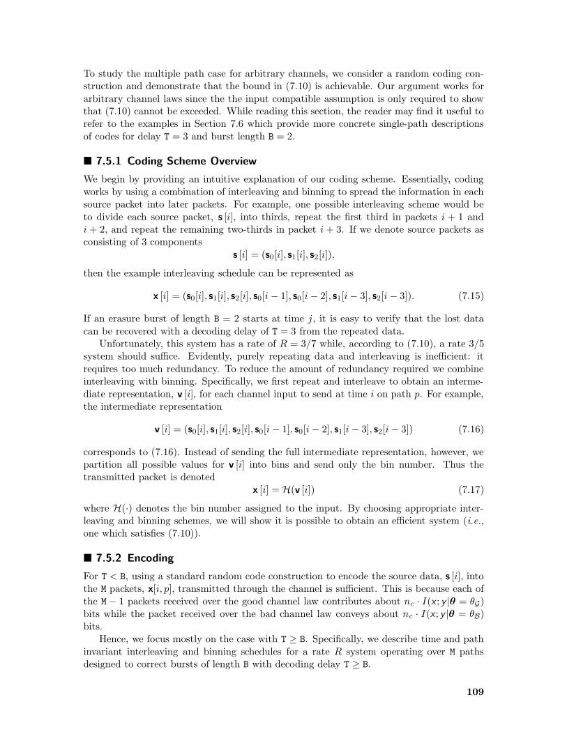
To study the multiple path case for arbitrary channels, we consider a random coding con-struction and demonstrate that the bound in (7.10) is achievable. Our argument works for

arbitrary channel laws since the the input compatible assumption is only required to showthat (7.10) cannot be exceeded. While reading this section, the reader may find it useful torefer to the examples in Section 7.6 which provide more concrete single-path descriptions

of codes for delay T = 3 and burst length B = 2.

� 7.5.1 Coding Scheme Overview

We begin by providing an intuitive explanation of our coding scheme. Essentially, coding

works by using a combination of interleaving and binning to spread the information in eachsource packet into later packets. For example, one possible interleaving scheme would be

to divide each source packet, s [i], into thirds, repeat the first third in packets i + 1 andi + 2, and repeat the remaining two-thirds in packet i + 3. If we denote source packets asconsisting of 3 components

s [i] = (s0[i], s1[i], s2[i]),

then the example interleaving schedule can be represented as

x [i] = (s0[i], s1[i], s2[i], s0[i− 1], s0[i− 2], s1[i− 3], s2[i− 3]). (7.15)

If an erasure burst of length B = 2 starts at time j, it is easy to verify that the lost data

can be recovered with a decoding delay of T = 3 from the repeated data.Unfortunately, this system has a rate of R = 3/7 while, according to (7.10), a rate 3/5

system should suffice. Evidently, purely repeating data and interleaving is inefficient: it

requires too much redundancy. To reduce the amount of redundancy required we combineinterleaving with binning. Specifically, we first repeat and interleave to obtain an interme-

diate representation, v [i], for each channel input to send at time i on path p. For example,the intermediate representation

v [i] = (s0[i], s1[i], s2[i], s0[i− 1], s0[i− 2], s1[i− 3], s2[i− 3]) (7.16)

corresponds to (7.16). Instead of sending the full intermediate representation, however, wepartition all possible values for v [i] into bins and send only the bin number. Thus thetransmitted packet is denoted

x [i] = H(v [i]) (7.17)

where H(·) denotes the bin number assigned to the input. By choosing appropriate inter-leaving and binning schemes, we will show it is possible to obtain an efficient system (i.e.,one which satisfies (7.10)).

� 7.5.2 Encoding

For T < B, using a standard random code construction to encode the source data, s [i], intothe M packets, x[i, p], transmitted through the channel is sufficient. This is because each of

the M− 1 packets received over the good channel law contributes about nc · I(x ; y |θ = θG)bits while the packet received over the bad channel law conveys about nc · I(x ; y |θ = θB)

bits.Hence, we focus mostly on the case with T ≥ B. Specifically, we describe time and path

invariant interleaving and binning schedules for a rate R system operating over M pathsdesigned to correct bursts of length B with decoding delay T ≥ B.

109

Dividing Source Packets

First, we divide each source packet at time i, s [i], into M pieces and associate each piecewith one possible path to obtain s[i, p] with p ∈ {0, 1, . . . , M−1}. Next we further sub-divide

each s[i, p] into L pieces denoted sj [i, p] with

L∆= T · M + B · (M− 1) + 1. (7.18)

We placenc · [I(x ; y |θ = θB)− ε] (7.19)

bits in the last piece, sL−1[i, p], for each path and evenly distribute the rest of the source

data among the remaining pieces yielding

nc ·CB,T − M · I(x ; y |θ = θB)− ε

L− 1(7.20)

bits for each piece sj [i, p] with j ∈ {0, 1, . . . , L− 2}. This splitting scheme is summarized inTable 7.1.

Table 7.1. Each source packet is split into M · L pieces. The number of bits for the last piece on each pathis specified by (7.19) and the size for the remaining pieces are specified in (7.20).

s [i]∆=

s0[i, 0] s1[i, 0] . . . sL−1[i, 0]s0[i, 1] s1[i, 1] . . . sL−1[i, 1]

......

......

s0[i, M− 1] s1[i, M− 1] . . . sL−1[i, M − 1]

Interleaving the Divided Packets

The pieces of each source packet are then interleaved to produce the intermediate represen-tation v[i, p] as specified in Table 7.2 and discussed in more detail below. The interleavingschedule is easiest to understand if we imagine that the transmitter “knows” a burst of

length B will start at time i on path p and designs an interleaver to allow quick recovery.Specifically, only s[i, p], s[i+1, p], . . ., s[i+B−1, p] are affected by the burst, therefore these

are the components considered by the interleaver inside the outermost for loop in Table 7.2.

Packets which follow the burst can communicate at most I(x ; y |θ = θG) bits of informa-tion while packets damaged by the burst can communicate at most I(x ; y |θ = θB) bits. One

approach to coding is to choose an interleaving schedule such that the receiver can recoversL−p−1[i] from y [i, p], and recover the remaining L− 1 pieces from the packets not suffering

the burst. But how many pieces of s [i] should be placed in later packets?

To answer this question, note that for a system transmitting at the burst-delay capacity,each of the packets transmitted on the M possible paths contains ncCB,T/M bits of new

information. Thus if a packet is received over the good channel state after the burst,the difference between the mutual information and the amount of new information sent is

110

Table 7.2. Description of how s [i]’s are interleaved to produce v[i, p]’s.

1: for p ∈ {0, 1, . . . , M− 1} do2: for l ∈ {0, 1, . . . , L− 1} do3: Put sl[i, p] in v[i, p]

4: end for5: for b ∈ {0, 1, . . . , B− 1} do

6: for m ∈ {0, 1, . . . , M− 1} do7: j ← b + mB

8: i′ ← i + T

9: p′ ← p + m mod M

10: Put sj [i, p] in v[i′, p′]

11: end for12: end for13: for t ∈ {0, 1, . . . , T− B− 1} do

14: j ← BM + t15: i′ ← i + t

16: for b ∈ {0, 1, B− 1} do17: Put sj [i, p] in v[i′ + 1 + b, p]18: end for

19: end for20: for t ∈ {0, 1, . . . , T− 1} do

21: for m ∈ {0, 1, . . . , M− 2} do22: j ← B(M− 1) + T + t + mT

23: i′ ← i + t

24: p′ ← p + 1 + m mod M

25: for b ∈ {0, 1, B− 1} do

26: Put sj[i, p] in v[i′ + b, p′]27: end for28: end for

29: end for30: end for

111

roughly

nc · [I(x ; y |θ = θG)− CB,T/M] = nc ·B

(T + B) · M · [I(x ; y |θ = θG)− I(x ; y |θ = θB)]. (7.21)

Thus, the amount of information about packets affected by the burst which can be recoveredby a packet following the burst is exactly (7.21). Stated differently, each packet can carry

about nc ·CB,T/M bits of new information in addition to the amount specified by (7.21) whichis used to carry redundant information about past data. For T > B, each packet sent at time

i + T will be received regardless of which path it takes. Therefore, we can start by placingthe maximum amount of redundant information from s [i] in the transmitted packets at

time i + T. Dividing the room left for redundant information in each packet (7.21) by thesize of pieces 0 through L− 2 (7.20) indicates that B pieces can be placed in each packet attime i + T. This explains step 10 of Table 7.2.

Next, since the transmitter “knows” packets x[i, p] through x[B − 1, p] will be lost inthe burst, there are T + 1 − B packets remaining on path p to which we can interleave

information. Therefore we interleave one piece of redundant information to each such v[i, p]input in step 17. (The loop in step 16 also interleaves the same piece to each of the preceding

B packets v[i, p], but this will be discussed later). Similarly, there are (M− 1)(T+ B) packetson the paths not affected by the burst within the decoding delay window which have not yetbeen assigned redundant information. Thus we assign each of these a different redundant

piece in step 26. (Again the loop in step 25 also interleaves the same piece to each ofthe preceding v[i, p]). This accounts for all pieces of s[i, p] except sL−1[i, p] which is not

interleaved at all.

Of course, the transmitter knows neither when the burst will start nor what path it

will strike. Therefore, the encoder essentially repeats the previous interleaving scheme withB possible time shifts and M possible path shifts. The time shifts explain the for loops insteps 16 and 25 mentioned earlier while the path shift explains the outermost for loop.

Binning the Interleaved Pieces

The interleaving schedule described above requires too much redundancy to be efficient by

itself. Therefore, instead of sending each v[i, p], we send only the bin index of each packet.Specifically, we define a hash partition with output length N as a mapping

H(·) : S∗ 7→ {0, 1}N (7.22)

which takes as input an arbitrary length sequence of source symbols from the alphabet Sand returns N bits. Instead of describing the a hash partition with a specific input–outputrelationship, we work with random hash partitions where every possible input is assigned a

random N -bit output.3 To construct burst-delay capacity achieving systems, we use randomhash partitions with output length

nc · [I(x ; y |θ = θG)− ε]/M (7.23)

and transmit the channel input x[i, p] by selecting codeword number H(v[i, p]) from a ran-dom channel codebook.

3By this we mean that the input–output relationship is randomly constructed not that H(s) may producedifferent random values when called with the same fixed input s.

112

Encoder Summary

To summarize, the encoding process is as follows. For each time i and each path p, arate 2nc(R)/M, length nc, random codebook is constructed by selecting 2nc(R)/M sequences of

length nc according to the i.i.d. distribution ps(·). Each source packet, s [i] is divided andinterleaved as described in Tables 7.1 and 7.2 to produce the intermediate representations

v[i, p]. A bin index, H(v[i, p]) is computed and the corresponding codeword in the codebookfor time i and path p is transmitted through the channel.

� 7.5.3 Decoding

To decode s [i], the receiver first decodes the bin indexes from the channel output and thendecodes the pieces of the source from the bin indexes. For packets received over the goodchannel state, decoding the bin index for x[i, p] is accomplished by looking for a codeword

jointly typical with the channel output y[i, p]. This will succeed with high probabilityaccording to standard arguments since the transmitted rate is less than the mutual infor-

mation. Furthermore, since the codebooks at each time and path are independent there areno error propagation or other dynamic issues in decoding the bin indexes.

Therefore, the main effort in describing and analyzing the decoding process is in decoding

the pieces of the source packets from the bin indexes. Essentially, the decoder accomplishesthis by trying to find a sequence of source packets jointly typical with the decoded bin

indexes. If a unique source packet is jointly typical it is declared to be s [i], otherwise adecoding error occurs. For simplicity, we consider a suboptimal bin decoding process whichnonetheless achieves capacity.

The analysis of the decoding process is somewhat lengthy and complicated. Hence thereader may find it useful to read the examples in Section 7.6 either before or in concert with

the rest of this section.

Decoding When No Burst Occurs

Lemma 1. When no burst occurs, s[i, p] can be decoded from y[i, p] with probability of errortending to zero as nc → 0.

Proof. Assume for the time being that all past source packets have been successfully re-

covered. With this assumption, decoding s [i] from the bin indexes obtained from x[i, p] forp ∈ {0, 1, . . . , M − 1} is straightforward. Specifically, while each v[i, p] includes data fromcurrent and past source packets, the past source data in v[i, p] is known by assumption and

can be ignored. Thus the unknown pieces are exactly the R ·nc bits of s [i]. Since we have M

bin indexes each consisting of nc ·I(x ; y |θ = θG)−ε]/M bits, the probability that an incorrect

source packet will be jointly typical with all the bin indexes is exactly

2nc·R · 2−nc·I(x ;y |θ=θG)−ε] = 2−nc[I(x ;y |θ=θG)−ε−R] (7.24)

which goes to zero asymptotically with nc for any ε > 0 provided R ≤ CB,T. The correctsource packet will always be jointly, and hence the probability of decoding error given the

past source data was correctly decoded and the current channel output was received overthe good channel state is approximately (7.24).4

4We say approximately and not exactly since the true probability of error must also take into accountthe possibility that the bin indexes are incorrectly decoded from the channel outputs. For R ≤ CB,T, thisprobability goes to zero so our approximation is justified. A sharper analysis, e.g., one which analyzes errorexponents, would need to take this into account, however.

113

Finally, we address the assumption that all past source packets have been successfullydecoded. This is trivially true for the initial packet and therefore our argument shows the

first packet can be successfully decoded with some small error probability ε′. Thus ourassumption is true for the second packet which can be decoded with a probability of errorat most 2ε′. Continuing by induction shows that the error probability for the nth packet is

no more than n · ε′. Thus the error probability for all the packets can be made negligibleprovided that ε′ decreases faster than n.

One way to accomplish this is to make sure that the packet size nc grows fast enough(and hence the error probability ε′ drops fast enough) with n to ensure that the product nε′

goes to zero. Increasing nc with n may be sufficient to provide simple bounds on the error

probability when n is finite, but it is somewhat undesirable if n is large or even infinite.In general, it is possible to obtain an error probability ε′ which depends only on nc and is

independent of n. This is achieved either by a detailed analysis of error propagation or byconsidering a more complicated decoding scheme. For the latter, the receiver decodes s [i]by looking not only at the current channel output y [i] but at all past channel outputs. For

such decoding, the difference between the received mutual information and the transmitteddata increases with both nc and n and so the error probability does not grow with n. We

omit such an analysis since our focus is on the first order effect of delay. Understandingthe details of the probability of error is an interesting topic for future work, however, andmight have connections to [157].

Decoding When a Burst Occurs

Next we assume that decoding was successful before time i when a burst of length B startedon path p. At first we give up on decoding the packets, y[i, p], y[i + 1, p], . . ., y[i + B− 1, p],

which are affected by the burst and declare the corresponding bin indexes H(v[i, p]), H(v[i+1, p]), . . ., H(v[i + B − 1, p]) to be erased. The other bin indexes can still be successfullydecoded, however, according to standard arguments.

Our main tool in decoding the intermediate representations v[i, p] from the successfullyrecovered bin indexes is the following lemma proved in Appendix E.

Lemma 2. Consider a bin index, H(v[i, p]), where the only unknown source componentsare s[i, p] and at most B redundant pieces of the form sb[a, c] with 0 ≤ b ≤ L − 2 of size

(7.20). All of these source components can be recovered with error probability approachingzero as nc →∞.

The intuition for this result is that each packet received over the good channel state can

convey about nc · I(x ; y |θ = θG) bits. Piece s[i, p] takes about nc ·CB,T bits while each of theother unknown components has a size of about (7.20). Thus, as discussed in Section 7.5.2,nc ·I(x ; y |θ = θG) will be larger than the amount of data in the unknown source components

so an appropriately encoded system will be able to decode correctly.We begin by focusing on the B · (M− 1) bin indexes which are “parallel” with the burst

but not affected by it.

Lemma 3. Imagine that all source data packets are correctly decoded until a burst starts

at time i on path p and let p′ 6= p and t ∈ {0, 1, . . . , B − 1}. Then all received packets ofthe form y[i + t, p′] can be decoded to their bin indexes H(v[i + t, p′]) and the corresponding

bin indexes can be decoded to their intermediate representations v[i + t, p′] with negligibleprobability of error. Furthermore, the decoding delay is at most T.

114

Proof. The rate of each bin index is chosen to be less than the channel mutual informationI(x ; y |θ = θG). Therefore, the bin indexes H(v[i + t, p′]) can be recovered using standard

arguments. The unknown components in each bin index are s[i + t, p′] as well as at mostB other pieces of the form sb[a, c] with 0 ≤ b ≤ L − 2. This follows by construction andspecifically by Table 7.2.

In particular, only one component of s[i, p] is placed in each v[i, p′] in step 26 of Table 7.2so Lemma 2 can be applied to show that is H(v[i, p′]) decoded successfully. Similarly, only

one component of s[i+1, p] is placed in each v[i+1, p′]. Note, however, that a new componentof s[i, p] is also placed in v[i + 1, p′] along with the component of s[i, p] which was placed

in v[i, p′] due to the loop in step 25 of Table 7.2. Since this last component was recoveredwhen H(v[i, p′]) was decoded in the previous step we can treat it as known when decodingH(v[i + 1, p′]). Thus we can again apply Lemma 2 to show H(v[i + 1, p′]) is decoded.

In general, v[i + t, p′] contains t + 1 components from s[i, p], plus t components from

s[i + 1, p], plus t − 1 components from s[i + 2, p], and so on down to one component froms[i + t, p] for a total of (t + 2)(t + 1)/2 components. The key insight of this lemma isthat many of these components are repeated. Specifically, of the two components from

s[i + t− 1, p] in v[i + t, p′], one of these was recovered when H(v[i + t− 1, p′]) was decoded.Similarly, of the three components from s[i+ t−2, p′] in v[i+ t, p′], two were recovered when

H(v[i + t − 1, p′]) was decoded, and so on. Thus, v[i + t, p′] contains at most t unknownsource components. Since t ≤ B − 1 by assumption, Lemma 2 implies that the desiredintermediate representations can be decoded.

Next we consider the (T + 1− B) · M packets following the burst.

Lemma 4. Imagine that all source data packets are correctly decoded until a burst starts at

time i on path p and let t ∈ {0, 1, . . . , T+1−B} and p′ ∈ {0, 1, . . . , M−1}. Then all receivedpackets of the form y[i + B+ t, p′] can be decoded to their bin indexes H(v[i + B+ t, p′]) and

the corresponding bin indexes can be decoded to their intermediate representations v[i+ t, p′]with negligible probability of error. Furthermore, the decoding delay is at most T.

Proof. As in Lemma 3, each bin index can be decoded and the unknown components ineach v[i+ t, p′] contain components of the form s[i+ t, p′] as well as at most B other pieces of

the form sb[a, c] with 0 ≤ b ≤ L−2. Establishing this is slightly different than in, Lemma 3,however.

For all but the last packet, (i.e., for all t ∈ {0, 1, . . . , T + 1 − B} except t = T + 1 − B)the situation is essentially the same as for decoding the last set of packets in Lemma 3.

Specifically, each bin index H(v[i+ t, p′]) contains exactly B unknown source components inaddition to s[i + t, p′] because other source components from s[i, p], s[i, p], . . ., s[i + B− 1, p]

in H(v[i + t, p′]) have been recovered in previous steps.5

The last set of bin indexes, H(v[i + T− 1, p′]), each contain exactly B components from

s[i, p] added in step 10 of Table 7.2 along with s[i+T−1, p′] and previously recovered sourcecomponents. Thus Lemma 2 implies that successful decoding occurs except with negligibleprobability.

5The situation is essentially the same and not exactly because in Lemma 3 going from time i + a toi + a + 1 always added more unknown source components to the bin index to be decoded. In Lemma 4,however, going from time i + t to i + t + 1 results in the same number of unknown source components inthe bin index to be decoded. Also, only paths with p′ 6= p were considered in the former while all paths areconsidered in the latter.

115

The previous lemmas establish successful decoding for all components of sj [i, p] withj ≤ L− 1, while the following considers the last piece.

Lemma 5. Imagine that all source data packets are correctly decoded until a burst startsat time i on path p. Then sL−1[i, p] can be decoded with negligible probability of error with

a decoding delay of T.

Proof. According to the previous lemmas, after a delay of T (i.e., at time i + T + 1), all

the components of s[i, p] can be successfully decoded except possibly sL−1[i, p] which wenow consider. By construction in (7.19), sL−1[i, p] is of size nc · [I(x ; y |θ = θB) − ε] bits.

Therefore, there are2nc·[I(x ;y |θ=θB)−ε] (7.25)

possible values for sL−1[i, p] and similarly, the number of possibilities for x[i, p] is also (7.25).The decoder searches for an x[i, p] which is jointly typical with the received channel output

y[i, p]. The correct codeword will be typical with high probability, while the probabilitythat a given incorrect codeword is typical is roughly 2−ncI(x ;y |θ=θB). Thus the probability

that any incorrect codeword is typical is about

2nc·[I(x ;y |θ=θB)−ε] · 2−ncI(x ;y |θ=θB) = 2−ncε. (7.26)

Thus decoding is successful with asymptotically negligible probability of error.

Combining all our results for this section yields the following theorem.

Theorem 23. Any rate less than the burst-delay capacity in (7.10) is achievable with de-coding delay T.

Proof. Lemmas 3, 4, and 5 imply that s[i, p] can be recovered with delay T when a burstof length B starts at time i on an arbitrary path p. Since the encoding scheme used is

time invariant, the same argument shows that all packets affected by the burst can also berecovered with delay T.

� 7.6 Single Path Examples

� 7.6.1 An Erasure Channel Example

Imagine that we which to design a system to correct for erasure bursts of length B = 2,

with decoding delay T = 3, using M = 1 path. Specifically, the good channel corresponds toa noiseless binary channel (i.e., I(x ; y |θ = θG) = 1) and the bad channel is a binary erasure

channel, (i.e., I(x ; y |θ = θB) = 0). According to (7.10), the burst-delay capacity is 3/5.Thus if each packet transmitted through the channel contains nc bits, then about (3/5)nc

source bits per packet can be reliably communicated.

Based on the coding scheme described in Section 7.5.2 each source packet should bedivided into L = 4 pieces, but since according to (7.19) the last piece is empty we ignoreit in this example. Thus each s [i] is divided into the three pieces (s0[i], s1[i], s2[i]) with

each piece consisting of about nc/5 bits. Applying the prescription in Section 7.5.2 andin particular the interleaving schedule in Table 7.2 produces the packet stream shown in

Table 7.3.

If all packets before time i are received correctly and x [i] and x [i + 1] are lost in burstof length 2, decoding proceeds as follows. At time i + 2, the decoder receives x [i + 2] and

116

Table 7.3. Encoding example for a rate R = 3/5 single path code. Each source componentis split into 3 equal pieces and interleaved. Instead of transmitting the interleaved datadirectly, a binning function H5/7(·) maps (7/5−ε)·nc input bits to a bin number consistingof nc bits.

x [i− 1] = H5/7

(s0[i− 1], s1[i− 1], s2[i− 1], s0[i− 2], s0[i− 3], s1[i− 4], s2[i− 4]

)

x [i + 0] = H5/7

(s0[i + 0], s1[i + 0], s2[i + 0], s0[i− 1], s0[i− 2], s1[i− 3], s2[i− 3]

)

x [i + 1] = H5/7

(s0[i + 1], s1[i + 1], s2[i + 1], s0[i + 0], s0[i− 1], s1[i− 2], s2[i− 2]

)

x [i + 2] = H5/7

(s0[i + 2], s1[i + 2], s2[i + 2], s0[i + 1], s0[i + 0], s1[i− 1], s2[i− 1]

)

x [i + 3] = H5/7

(s0[i + 3], s1[i + 3], s2[i + 3], s0[i + 2], s0[i + 1], s1[i + 0], s2[i + 0]

)

x [i + 4] = H5/7

(s0[i + 4], s1[i + 4], s2[i + 4], s0[i + 3], s0[i + 2], s1[i + 1], s2[i + 1]

)

searches for a collection of pieces

(s0[i + 2], s1[i + 2], s2[i + 2], s0[i], s0[i + 1]) (7.27)

which has a bin number corresponding to x [i + 2]. The correct collection will always havethe correct bin number. The probability that an incorrect collection has the correct bin

number is 2−nc . Since the correct value for s [i− 1] is known and each unknown source piececonsists of about ncR/3 bits, there are 2(5/3)ncR possible collections. Thus the expected

number of incorrect collections which nonetheless have the correct bin number is

2−nc · 2nc(5/3)R = 2−nc[1−(5/3)R].

Thus provided that R < 3/5 − ε, the expected number of incorrect collections which havethe correct bin number is at most 2−nc(5/3)ε and the probability of decoding failure goes to

zero as nc →∞.

Similarly, when x [i + 3] is received the decoder searches for a collection of pieces

(s0[i + 3], s1[i + 3], s2[i + 3], s0[i + 1], s0[i + 2], s1[i], s2[i])

which has a bin number matching x [i + 3]. Provided that s0[i+1] and s [i + 2] were correctlydetermined in the preceding step, the probability that an incorrect collection has the correct

bin number will be small according to the previous argument. Thus, with probabilityarbitrarily close to 1, the decoder will correctly recover the lost packets.

� 7.6.2 A Single Path Binary Symmetric Channel Example

Next consider a noiseless binary channel as the good channel and a binary symmetric channel

with cross-over probability p as the bad channel. If p is chosen such that Hb(p) = 1/3where Hb(·) denotes the binary entropy function, then the only difference as compared tothe erasure channel example is that now I(x ; y |θ = θB) = 1 −Hb(p) = 2/3 and therefore

each source packet is split into 4 pieces where the last piece contains (2/3− ε) · nc bits andthe remaining 3 pieces each contain (1/15− ε) · nc bits. The total amount of bits in each

source packet is(3/15 + 2/3− 4ε)nc = (13/15− 4ε)nc (7.28)

117

bits which equals the bound (7.10) for successful decoding of bursts of length B = 2 withdelay T = 3:

CB,T =3

5+

2

5· (1−Hb(p)) =

3

5+

2

5· 23

=13

15.

Applying the interleaving schedule described in Table 7.2 produces the packet streamshown in Table 7.4.

Table 7.4. Encoding example for a burst binary symmetric channel. Each source packet issplit into four pieces and interleaved. Instead of transmitting the interleaved data directly,a binning function, H15/17(·) maps (17/15 − 8ε)nc input bits to a bin number consistingof nc bits.

x [i− 1] = H15/17

(s0[i−1], s1[i−1], s2[i−1], s3[i−1], s0[i−2], s0[i−3], s1[i−4], s2[i−4]

)

x [i + 0] = H15/17

(s0[i+0], s1[i+0], s2[i+0], s3[i+0], s0[i−1], s0[i−2], s1[i−3], s2[i−3]

)

x [i + 1] = H15/17

(s0[i+1], s1[i+1], s2[i+1], s3[i+1], s0[i+0], s0[i−1], s1[i−2], s2[i−2]

)

x [i + 2] = H15/17

(s0[i+2], s1[i+2], s2[i+2], s3[i+2], s0[i+1], s0[i+0], s1[i−1], s2[i−1]

)

x [i + 3] = H15/17

(s0[i+3], s1[i+3], s2[i+3], s3[i+3], s0[i+2], s0[i+1], s1[i+0], s2[i+0]

)

x [i + 4] = H15/17

(s0[i+4], s1[i+4], s2[i+4], s3[i+4], s0[i+3], s0[i+2], s1[i+1], s2[i+1]

)

If all packets before time i are received correctly and x [i] and x [i + 1] are lost in burstof length 2, decoding proceeds as follows. At time i + 2, the decoder receives x [i + 2] andsearches for a collection of pieces

(s0[i + 2], s1[i + 2], s2[i + 2], s3[i + 2], s0[i], s0[i + 1]) (7.29)

which has a bin number corresponding to x [i + 2]. The correct collection will always havethe correct bin number. The probability that a given incorrect collection has the same bin

number as x [i + 2] is 2−nc. Since the correct value for s [i− 1] is known, there are

2nc·(13/15−4ε) · 2nc·(1/15−ε) · 2nc·(1/15−ε) = 2nc(1−6ε)

possible collections, i.e., the cardinality of s [i + 2], s0[i], and s0[i + 1]. Thus the expectednumber of incorrect collections which nonetheless have a bin number matching x [i + 2] is

2−nc · 2nc(1−6ε) = 2−6ncε.

Thus the probability of decoding failure goes to zero as nc →∞.Similarly, when x [i + 3] is received the decoder searches for a collection of source com-

ponents which has a bin number matching x [i + 3]. Provided that s0[i + 1] and s [i + 2]were correctly determined in the preceding step, the probability that an incorrect collectionhas this bin number will be small. Specifically, the unknown components in x [i + 3] are

(s0[i + 3], s1[i + 3], s2[i + 3], s3[i + 3], s1[i], s2[i]) (7.30)

because s0[i + 2] and s0[i + 1] were recovered when x [i + 2] was decoded. Thus, accordingto the previous argument x [i + 3] is decoded.

Finally, having decoded s0[i], s1[i], and s2[i] the receiver can decoded s3[i] by searchingfor a sequence s3[i] jointly typical with y [i] and the previously decoded terms. There are

118

2nc(2/3−ε) possible values for s3[i]. The codeword corresponding to the correct value of s3[i]will be jointly typical with high probability. The probability that a given (incorrect) value

of s3[i] is jointly typical with the channel output y [i] is roughly 2−ncI(x ;y |θ=θB). Thus theexpected number of incorrect codewords which are jointly typical with y [i] is roughly

2nc[I(x ;y |θ=θB)−ε−I(x ;y |θ=θB)] = 2−ncε.

Thus, with probability arbitrarily close to 1, only the transmitted sequence s3[i] will be

jointly typical and decoding will succeed.

This examples illustrates an interesting (and probably essential) feature of our encodingand decoding process: only a subset of the information from s [i] is repeated in later packets.

When a burst occurs at time i, the decoder does not try to recover all of x [i] from laterpackets. Instead, the decoder recovers just enough of x [i] from later packets to decrease

the uncertainty about x [i] to a point where it can be resolved from the output of the badchannel.

� 7.7 Practical Coding Schemes

The random coding schemes presented so far are too complex to be implemented, butthe random codes suggest how practical, structured codes can be designed. As illustrated

by the examples in Section 7.6.1 and Section 7.6.2, our coding scheme has a componentthat is based only on the decoding delay and burst length and a component based only

upon the channel mutual informations in the good and bad state. The former correspondsto interleaving and binning scheme while the latter corresponds to using familiar randomcodes for a noisy channel. It seems that these components are almost separable.

Based on recent success in practical constructions of single path burst erasure cor-recting codes [119] via Reed-Solomon codes, we suspect this insight has some interestingpractical implications. Specifically, we believe that burst-delay capacity achieving codes for

non-erasure channels can be designed by combining inner codes for traditional non-burstychannels with outer codes designed for a burst erasure channel. Decoding would work by

first using the inner decoder on packets arriving over the good channel and treating packetsarriving over the bad channel as erased. Next components 0 through L− 2 of the “erased”information sources would be decoded. Finally, all previously decoded information could

be used as side information for the inner decoder used to recover packets arriving over thebad channel.

For example, consider a bursty, additive white Gaussian noise channel. One appropriate

inner code would be a multi-level Gaussian code where one level (or set of levels) conveysabout I(x ; y |θ = θB) bits per sample and the other level (or set of levels) conveys about

I(x ; y |θ = θG) bits per channel. The outer code would be a burst-delay capacity achievingcode for an erasure channel with the same T and B. First, all source components for sj [i]except sL−1[i] would be decoded from the outer erasure correcting code. The resulting

information would correspond to the second set of levels for the multi-level Gaussian code.“Subtracting off” this known information from the multi-level Gaussian code, would then

leave a Gaussian code conveying about I(x ; y |θ = θB) bits per sample of information whichcould be successfully decoded on the bad channel.

119


In this chapter we have considered streaming information over bursty channels. We intro-duced an adversarial channel model where nominally each packet is received over a good

channel while an occasional burst of B packets are received over a bad channel. One ad-vantage of this adversarial model is that it requires a less precise channel model and hencemay be more robust to the difficulties of accurate channel measurement. More importantly,

however, our adversarial burst model provides a nice setting to study and illustrate therelationship between channel dynamics and code structure.

Specifically, if we require that each source packet can be decoded with a delay of at mostT packets, then a natural quantity of interest is the maximum amount of information whichcan be reliably communicated. In order to derive a coding theorem characterizing this

burst-delay capacity, we introduced a new type of random coding argument which spreadsinformation over time in a way which depends on the burst length and decoding delay. We

believe that this type of random coding argument may be an essential tool in understandingthe fundamental delay introduced in a variety of channel models both bursty and otherwise.

120

Chapter 8

Delay-Optimal Burst Erasure CodeConstructions

121

In this chapter we describe how to construct codes to meet the optimal burst-delaytrade-off in Chapter 7. We focus mainly on burst erasure channels, but such codes can also

be extended to other types of bursty channels as sketched in Section 8.5.


We consider the same problem model as in Chapter 7, but specialize it to erasure chan-nels and feedback-free linear codes with finite memory. As illustrated in Fig. 8-1 a lin-

ear, feedback-free, rate R = k/n, M path packet encoder, f(·), is a causal, multiple-input multiple-output, linear filter (i.e., a convolutional code). Specifically, the input tof(·) is a source stream, s [i], where each source symbol consists of k sub-symbols s [i] =

(s0[i], s1[i], . . . , sk−1[i]) each taking values over some finite field GF(q). The output of f(·)is a collection of encoded streams, x[i, p] (with p ∈ {0, 1, . . . , M − 1}) where each encoded

symbol consists of n sub-symbols over the same finite field GF(q). At time i, each x[i, p] istransmitted along the pth channel path. We consider bursts of length B where at any time,

i∗, B packets on any path, p∗, may be erased. A burst-delay optimal code is one which cancorrect any such burst with delay T where the parameters B, T, and R satisfy the trade-offderived in (7.10).

In this chapter, our goal is to construct such optimal codes with low encoding anddecoding complexity and the smallest possible field size. In practice, the maximum possible

packet size is determined by the underlying channel characteristics and is not a parameterwhich the code designer can change. For example, the coherence time in a wireless channel

or the Maximum Transmit Unit (MTU) in an Internet link might determine the maximumpacket size (and hence the maximum field size for the code). Thus if a burst-delay optimalcode with an alphabet size smaller than the maximum packet size exists, then the burst-

delay capacity in (7.10) can be practically achieved. Otherwise, finite length effects forcethe system to operate at a burst-delay-rate trade-off worse than the fundamental limit in

(7.10).

� 8.2 Single-Link Codes

We begin by focusing on single link codes and observe that designing packet encoders canbe viewed as essentially designing matched interleavers and block codes. Specifically, in

Fig. 8-1, the initial delay elements can be viewed as a periodic interleaving of the inputsimilar to [62]. Instead of working with the structure in Fig. 8-1 which requires us to

specify M block codes, we instead choose a different interleaving structure to simplify designof the corresponding block code.

In particular, to obtain a simple mapping between the properties of the convolutionalcode and the block code, we use the interleaving structure shown in Fig. 8-2. We refer tothis as “diagonal interleaving” both to distinguish it from Forney’s periodic interleaving [62]

and for another reason illustrated shortly. Furthermore, when discussing block code design,we denote the inputs and outputs of the block code as vj and wj and reserve the symbols

sj [i] and xj [i] for the input and output of the corresponding packet encoder obtained viainterleaving.

As stated in the following theorem and proved in Appendix F, diagonal interleavingallows us to construct a rate k/n convolutional code to correct any burst of length B with

delay T , by focusing on the somewhat simpler problem of constructing a single (n, k) blockcode.

122

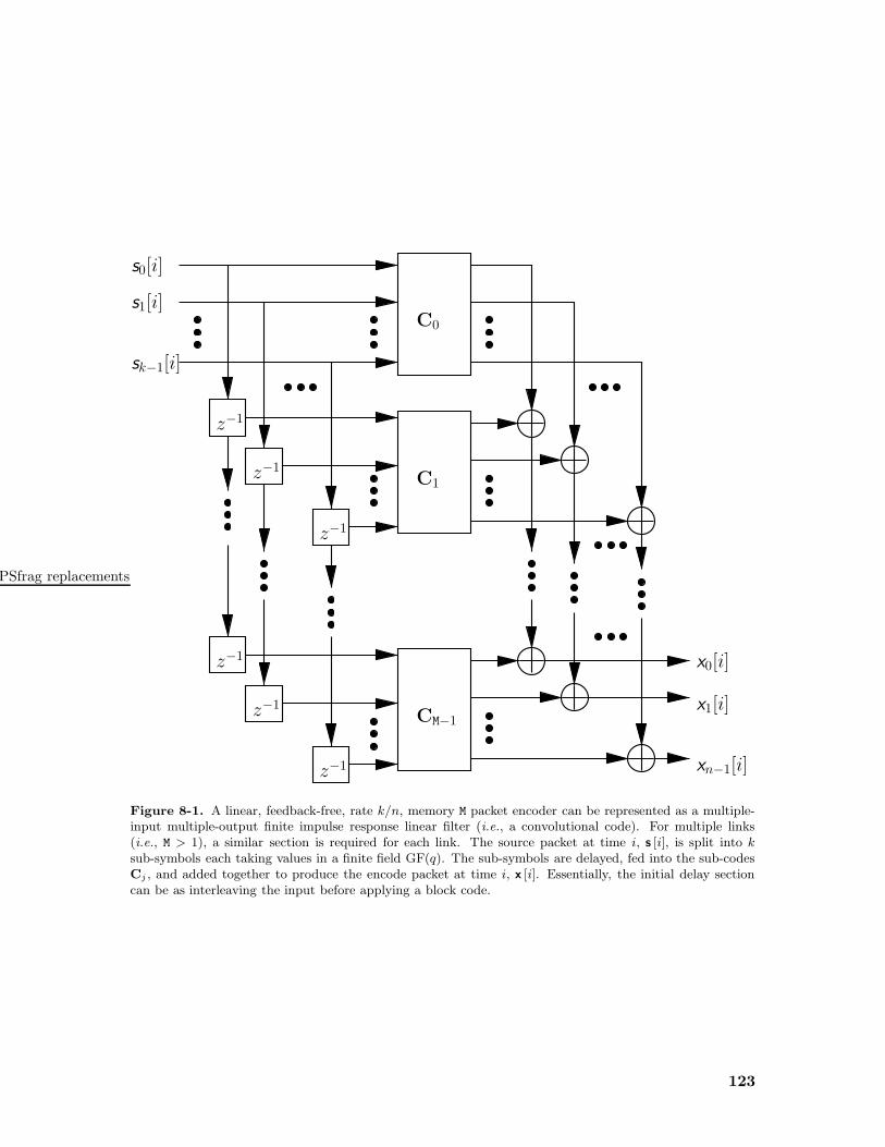
PSfrag replacements

z−1

z−1

z−1

z−1

z−1

z−1

s0[i]

s1[i]

sk−1[i]

x0[i]

x1[i]

xn−1[i]

C0

C1

CM−1

Figure 8-1. A linear, feedback-free, rate k/n, memory M packet encoder can be represented as a multiple-input multiple-output finite impulse response linear filter (i.e., a convolutional code). For multiple links(i.e., M > 1), a similar section is required for each link. The source packet at time i, s [i], is split into ksub-symbols each taking values in a finite field GF(q). The sub-symbols are delayed, fed into the sub-codesCj , and added together to produce the encode packet at time i, x [i]. Essentially, the initial delay sectioncan be as interleaving the input before applying a block code.

123

Theorem 24. Consider an (n, k) systematic block code, C, that can recover the ith inputsymbol from the unerased symbols from 0 through T + i for any erasure burst of length B.

Then such a code can be diagonally interleaved as in Fig. 8-2 to yield a rate k/n, single-link,packet encoder which can correct any erasure burst of length B with delay T.

PSfrag replacements

z−1

z−1

z−k+1

z−k+2

z

zk−1

zk−2

z−n+k

s0[i]

s1[i]

sk−2[i]

sk−1[i]

v2[i]

v2[i]

v2[i]

v2[i]

w0[i]

w1[i]

wk−2[i]

wk−1[i]

wk[i]

wn−1[i]

x0[i]

x1[i]

xk−2[i]

xk−1[i]

xk[i]

xn−1[i]

y0[i]

y1[i]

y2[i]

yn−1[i]

Sys

tem

atic

Blo

ckC

ode

Chan

nel

Figure 8-2. A convolutional code structure based on diagonal interleaving. The z−λ and zλ elementsdenote delay or advance by λ. Advances are possible since they can be “pushed through” the systematicblock code to cancel with delays.

An example best illustrates this idea. Imagine we want to construct a convolutional codeto correct all bursts of length B = 2 with delay T = 3. First, we construct the following

block code taking the input vector v to the output vector w via left multiplication by acode matrix C:

w = v ·C =(

v0 v1 v2

)·

1 0 0 1 0

0 1 0 0 10 0 1 1 1

=(

v0 v1 v2 v0 + v2 v1 + v2

)(8.1)

It is straight-forward to verify that if any two symbols in the code vector w are erased, thenthey can both be recovered with a delay of 3. For example if w1 and w2 are erased then the

latter can be recovered via w2 = w3⊕w0 and the former can be recovered via w1 = w4⊕w2.

Of course the block code in (8.1) does not satisfy our definition of a packet encoder (itcan only encode a single block and not a semi-infinite stream as required by our model).Therefore, to obtain a packet encoder, we interleave such a block code as in Fig. 8-2. The

effect of the interleaver is that parity check symbols are computed along “diagonals” of theconvolutional code as illustrated in Table 8.1. It is easy to show that if the constitunent

block code corrects any burst of length B with delay T then the corresponding convolutionalcode will also. Hence, we can simplify the convolutional code construction problem by only

124

Table 8.1. Illustration of how a rate 3/5 convolutinal code can be constructed by the interleaving structureof Fig. 8-2. Essentially, the block code is computed along the “diagonal” of the convolutional code. Boxedentries compromise one such constituent block code.

x [i] =(

s0[i] s1[i] s2[i] s0[i− 3]⊕ s2[i− 1] s1[i− 3]⊕ s2[i− 2])

x [i + 1] =(

s0[i + 1] s1[i + 1] s2[i + 1] s0[i− 2]⊕ s2[i] s1[i− 2]⊕ s2[i− 1])

x [i + 2] =(

s0[i + 2] s1[i + 2] s2[i + 2] s0[i− 1]⊕ s2[i + 1] s1[i− 1]⊕ s2[i])

x [i + 3] =(

s0[i + 3] s1[i + 3] s2[i + 3] s0[i]⊕ s2[i + 2] s1[i]⊕ s2[i + 1])

x [i + 4] =(

s0[i + 4] s1[i + 4] s2[i + 4] s0[i + 1]⊕ s2[i + 3] s1[i + 1]⊕ s2[i + 2])

considering block code constructions.

� 8.2.1 Reed-Solomon Codes Are Not Generally Optimal

Reed-Solomon codes (and other cyclic codes) are well-known to have excellent burst cor-recting properties when their delay is not considered. Thus, it might seem natural to usesuch codes in the periodic interleaving structure as suggested by Forney [62] or in the diag-

onal interleaving structure in Fig. 8-2. Unfortunately, such constructions are not generallyoptimal. For example, consider attempting to use a Reed-Solomon code in place of the code

of (8.1) to correct bursts of length 2 with delay 3. If the delay starts at time 0 and erases w0

and w1, then these symbols can not be recovered until all of them remaining code symbols

are received. Thus the Reed-Solomon construction requires a worst case delay of 4 insteadof 3 with either type of interleaving.

In general, the straightforward construction using an (n, k) Reed-Solomon code requiresa worse case delay of n − 1 to correct any burst of length n − k. In contrast, an (n, k)block code must correct any burst of length n− k with delay k if it is to yield a burst-delay

optimal code after interleaving.

� 8.2.2 Provably Optimal Construction For All Rates

As stated Theorem 25 and illustrated in Fig. 8-3, we can construct the required (n, k) block

code to interleave into a delay-optimal rate k/n burst correcting convolutional code bycombining a repetition block code and a block code which corrects bursts without regard

to delay.

Theorem 25. A rate k/n code capable of correcting any burst of length n− k with delay kcan be constructed by diagonally interleaving the matrix

G∗k×n =

(In−k×n−k 0n−k×2k−n In−k×n−k

02k−n×n−k Pcyc,2k−n×k

)

(8.2)

where Ii×j is an i-by-j identity matrix, 0i×j is an i-by-j zero matrix, and Pcyc,2k−n×k is the(2k− n)-by-k systematic generator matrix for a length k, dimension 2k− n code capable of

correcting any erasure burst of length at most n− k (including end-around bursts) withoutregard to delay.

125

��

��

��

��

�� !"#

$%&'()

*+,-./

PSfrag replacements (2n− 2k, n− k)

Repetition

Code

(k, 2k − n)

Systematic

Burst

Correcting

Code

v0

v0

v1

v1

vn−k−1

vk−1

vn−k

vn−k+1

v0 = w0

v1 = w1

vn−k−1 = wn−k−1

vn−k = wn−k

vn−k+1 = wn−k+1

vk−1 = wk−1

v0 ⊕ p0 = wk

v1 ⊕ p1 = wk+1

vn−k−1 ⊕ pk−1 = wn−1

p0

p1

pn−k−1

Figure 8-3. An (n, k) delay-optimal erasure burst correcting block code can be constructed by combininga repetition code and a code capable of correcting erasure bursts of length n − k without regard to delay.The encoder shown above maps the (interleaved) symbols v0, v1, . . ., vk−1 to the (interleaved) code symbolsw0, w1, . . ., wn−1.

126

Before proving Theorem 25, we illustrate how it can be applied to construct a rate7/11 code over GF(2) which is capable of correcting any burst of length 4 with delay 7.

The desired code requires a generator matrix Pcyc,7×3 corresponding to a (7, 3) erasureburst correcting code. We can obtain Pcyc,7×3 from a binary cyclic code generated byg(x) = x4 + x2 + x1 + 1. Thus the desired generator matrix for the rate 7/11 code is

1 0 0 0 0 0 0 1 0 0 00 1 0 0 0 0 0 0 1 0 00 0 1 0 0 0 0 0 0 1 0

0 0 0 1 0 0 0 0 0 0 10 0 0 0 1 0 0 1 1 1 0

0 0 0 0 0 1 0 0 1 1 10 0 0 0 0 0 1 1 1 0 1

. (8.3)

Proof of Theorem 25: As illustrated by Fig. 8-3 and the example code in (8.3), the first

n − k information symbols are treated quite differently than the last 2k − n informationsymbols. We refer to these two classes of information symbols as the urgent and non-urgentsymbols respectively since we can ignore the delay required in recovering the latter provided

they are eventually recovered but must insure the delay in recovering the former is at mostk. We first describe how the non-urgent symbols are decoded and then describe how the

urgent symbols are decoded.

Assume that an erasure burst of length n − k starts at time 0 ≤ i ≤ k − 1 (burstsstarting after time k − 1 are equivalent to bursts starting at time k − 1 since the bursts

after time k − 1 fall off the end of the code vector). By time at most i + k − 1, we wouldreceive exactly 2k−n cyclically consecutive1 symbols of the bottom block code in Fig. 8-3.Note that while repeated symbols from time 0 through i− 1 are added to the parity check

symbols of the bottom block code, these repeated symbols can be subtracted out of thedesired parity check symbols of the bottom block code because they are correctly received

before the burst. By assumption the bottom block code can decode any cyclic burst oflength n − k or equivalently any cyclically consecutive 2k − n symbols are an informationset. Thus by time i + k − 1 we can recover the non-urgent information symbols.

Once the non-urgent information symbols are recovered we can subtract the effect ofthe parity check symbols of the bottom block code in Fig. 8-3 from the top repetition code.Furthermore, note that this subtraction can be performed at time i+k−1 which is exactly

the time when the first urgent symbols must be recovered. Thus the first urgent informationsymbol is recovered from the repetition code at time i+k−1, the second urgent information

symbol is recovered from the repetition code at time i + k, and so on until the last urgentinformation symbol is recovered.

For example, consider the matrix in (8.3). If a burst started at time 2 then urgent

information symbols 0 and 1 would be received correctly as would the last non-urgentinformation symbol. The 2 urgent information symbols could then be subtracted out of thefirst 2 parity check symbols of the bottom block code. After this subtraction is performed,

at time 9 we have 3 consecutive symbols of the bottom (7, 3) code and thus the non-urgent information symbols are recovered. Once the non-urgent information symbols are

recovered, their effect on the repetition code at the top of Fig. 8-3 can be subtracted out.Thus information symbols 2, 3, and 4 would each be recovered with delay 7.

1By cyclically consecutive we mean that the code vector is assumed to wrap around. For example,symbols A—D in the code vector (A B ∗ ∗ C D) are cyclically consecutive.

127

At first glance, Theorem 25 may seem useless since applying it requires constructinga smaller burst correcting code. Since the smaller burst correcting code need only cor-

rect bursts without regard to delay, however, constructing it is generally much easier thandirectly constructing a low delay burst correcting code. In fact, if a cyclic code of theappropriate length and dimension exists for the desired alphabet then it suffices since any

(n, k) cyclic code can correct all erasure bursts of length n− k.2

For example, to construct a rate 5/8 code capable of correcting any burst of length 3with delay 5 we require the generator matrix for a (5, 2) code which can correct any burstof length 3 (without regard for delay). Since x5 +1 factors into (1+x) ·(1+x+x2+x3 +x4)

there is no binary cyclic code of dimension 2 and length 5.3 We could consider larger fieldsto find a cyclic code with the right parameters (e.g., a Reed-Solomon code over GF(5)). If

using a binary alphabet is important, we can use a (non-cyclic) binary code generated bythe following matrix:

Pcyc,2×5 =

(1 0 1 1 00 1 0 1 1

)

(8.4)

which we can verify by inspection can correct any erasure burst of length 3. Thus we obtain

the generator matrix for the desired rate 5/8 code

1 0 0 0 0 1 0 00 1 0 0 0 0 1 0

0 0 1 0 0 0 0 10 0 0 1 0 1 1 0

0 0 0 0 1 0 1 1

. (8.5)

In any case, if a cyclic code does not exist or is inconvenient to find, the requirederasure burst correcting code can always be constructed with a symbol alphabet that is not

too large.

Corollary 7. The largest alphabet size required for the generator matrix Pcyc,2k−n×k in

Theorem 25 is at most qm where qm is the smallest prime power exceeding k.

Proof. By constructing a Reed-Solomon code over GF(qm) and puncturing the code down

to length k we obtain an MDS code which can correct the desired erasure bursts.

Corollary 8. The largest alphabet size required for the generator matrix Pcyc,2k−n×k inTheorem 25 is at most 2k.

Proof. By applying Corollary 7 with q = 2 we see that the field size is at most the largestpower of 2 which is greater than or equal to k.

While there are clearly parameters for which no cyclic code exists, it would be interesting

to know whether there are parameters (n, k) where there is no binary block code capable ofcorrecting all erasure bursts of length (n− k) and moving to higher alphabets is absolutely

required.

2To see this, note that for a systematic cyclic code the first k symbols form an information set. Sinceany cyclic shift of a codeword is also a codeword, any consecutive k symbols must form an information set.

3A cyclic code of dimension k and length n over GF(2) exists if and only if xn + 1 has a factor of degreen − k over GF(2) [108].

128

� 8.3 Two-Link Codes

In this section we consider scenarios where the transmitter can use two links as illustrated

in Fig. 8-4. Intuitively, the advantage of using multiple links is that the extra links canreduce the delay required to correct for a given burst length and coding rate. In particular,

it is possible to lower bound the ratio of decoding delay to correctable burst length via

T

B≥{

max[

1M· 1

1−R − 1, 1]

, R ≥ M−1M

0, R ≤ M−1M

(8.6)

or equivalently to upper bound the code rate via

R ≤{

1− B

(T+B)·M , T ≥ B

1− 1M, T < B.

(8.7)

As we see from (8.6) doubling the number of transmission links almost halves the decodingdelay confirming our intuition about the value of multiple links.

PSfrag replacements

s [i]

x1[i]

x2[i]

y1[i]

y2[i]

Ch. 1

Ch. 2

Encoder Decoder

Figure 8-4. A channel with two transmission links.

� 8.3.1 Constructions

To construct delay optimal convolutional codes for the two-link case we again use the idea

of interleaving block codes as illustrated in Table 8.2. To construct a delay optimal con-volutional code we can instead solve the simpler problem of constructing a delay optimalblock code. Notice that in contrast to the single-link case, however, the block code for a

multi-link channel has multiple samples for a given “time slot”. Perhaps a good way todenote such a block code is to write the output for link j as wj and represent the encoding

operation as(

w1 w2

)= v ·

(C1 C2

)=(

v ·C1 v ·C2

)(8.8)

where the || is intended to convey the idea that w1 and w2 are code vectors which are sentat the same time but on different links.

With this notation, the constituent block code in Table 8.2 would have

C1 =

1 0

0 10 0

and C2 =

0 1

0 11 1

with v =(

v0 v1 v2

)(8.9)

129

Table 8.2. Illustration of how a two-link convolutional code can be constructed by using a block codeon the diagonal. Boxed entries compromise a constituent block code. The code shown is a rate 3/4code capable of correcting any burst of length B = 1 with decoding delay T = 1 and is therefore optimalaccording to (8.6).

y0[i] =(

s0[i] s1[i]) (

s2[i] p1[i])

y1[i] =(

s0[i + 1] s1[i + 1]) (

s2[i + 1] p1[i + 1] = s0[i]⊕ s1[i + 1]⊕ s2[i])

resulting in the two-link block code

(w1 w2

)=(

v ·C1 v ·C2

)=

(v0 v2

v1 v0 ⊕ v1 ⊕ v2

)

. (8.10)

Fig. 8-5 illustrates how our code construction can be extended to the case of two links.As stated Theorem 26 (and proved in Appendix F), we can obtain a block code to interleave

into a two-link, delay-optimal, rate k/n, burst correcting convolutional code by combiningsmaller delay-optimal single-link codes.

Theorem 26. Consider positive integers k and n with n even and k/n ≥ 3/4. A rate k/ntwo-link code capable of correcting any burst of length B = (n− k) with delay T = (k− n/2)

can be constructed by diagonally interleaving the matrix G∗∗k×n = (G(∗∗,1)k×n ||G

(∗∗,2)k×n ) where

G(∗∗,1)k×n =

(In/2×n/2

0(k−n/2)×n/2

)

, G(∗∗,2)k×n =

G(∗,0)(k−n/2)×n/2

0(n−k)×(k−n/2) I(n−k)×(n−k)

G∗(k−n/2)×n/2

, (8.11)

and G(∗,0)a×b is a generator for the single-link code construction in Theorem 25 with the upper

left identity matrix replaced by zeros, and the remaining notation the same as in Theorem 25.

Some discussion and examples help clarify Theorem 26. First, note that restricting n

to be even is only used to simplify the exposition and does not restrict the possible rates.For example, to obtain a rate 4/5 code, one could use the parameters k = 8 and n = 10

in Theorem 26. Second, the restriction that k/n ≥ 3/4 causes no difficulty in achievingthe bound in (8.6). To see this note that for rates less than 3/4, the two-link boundyields T/B ≥ 0 which is trivially achieved by sending exactly the same data on both links.

Evidently, only codes with R = 1/2 or R ≥ 3/4 are sufficient. Finally, observe that by settingR = k/n and M = 2 in (8.6) we obtain T/B ≥ (k − n/2)/(n− k) so the codes in Theorem 26

are optimal.

To gain some insight into the structure of the two-link construction we consider a rate4/5 example. For this rate, we choose n = 10 and k = 8 to obtain a code capable of

correcting any burst of length 2 with delay 3. To obtain codes correcting longer bursts, wecould multiply this k and n by any positive integer.

According to Theorem 26, this code requires the matrix G∗3×5 corresponding to a (5, 3)single-link, delay-optimal, erasure burst correcting block code. Using Theorem 25 we obtain

130

��

��

� ��

��

��

�� !�!"#�#$

%�%&'�'()�)*

+�+,-�-./�/0

123456

PSfrag replacements Optimal (n/2, k − n/2)

Single-Link Encoder

Optimal (n/2, k − n/2)

Single-Link Encoder

v0

w1,0

v1

w1,1

vk−n/2−1

w1,k−n/2−1

vk−n/2

w1,k−n/2

vk−n/2+1

w1,k−n/2+1

vn/2−1

w1,n/2−1

vn/2

w2,0

vn/2+1

w2,1

vk−1

w2,k−n/2−1

w2,k−n/2

w2,k−n/2+1

w2,n/2−1

Figure 8-5. An (n, k) two-link, delay-optimal, erasure burst correcting, block code correcting any burst oflength n−k with delay k−n/2 can be constructed by combining two single-link, (k−n/2, n/2) delay-optimal,erasure burst correcting, block codes. The encoder shown above maps the k (interleaved) symbols v0, v1,. . ., vk−1 to the n (interleaved) code symbols w1,0, w1,1, . . ., w1,n/2−1 and w2,0, w2,1, . . ., w2,n/2−1. Thesystematic output symbols of each single-link code are shown vertically and the parity output symbols areshown horizontally. Note that the first code stream w1,0, w1,1, . . ., w1,n/2−1 is simply composed of the firstn/2 − 1 input symbols and so the systematic output symbols of the top single-link code are unused.

131

G∗3×5 =

1 0 0 1 00 1 0 0 1

0 0 1 1 1

. (8.12)

Thus the encoding matrix for the two-link block code is

G∗∗8×10 =

1 0 0 0 0 0 0 0 1 0

0 1 0 0 0 0 0 0 0 10 0 1 0 0 0 0 0 1 1

0 0 0 1 0 0 0 0 1 00 0 0 0 1 0 0 0 0 10 0 0 0 0 1 0 0 1 0

0 0 0 0 0 0 1 0 0 10 0 0 0 0 0 0 1 1 1

. (8.13)

Let us consider the burst correcting capabilities of G∗∗8×10. As illustrated by Fig. 8-5 and

the encoding matrix in (8.13), the idea behind this construction is that if a burst occurson the second stream, we strip out the information received on the first stream so that thesecond stream looks like a single-link code suffering a correctable burst. A similar stripping

argument can be used if a burst occurs on the first stream. This intuition is made preciseby considering bursts on each stream in detail as follows.

Imagine an erasure burst of length 2 occurs on the second stream. Without loss ofgenerality, we can assume that the data symbols on the first stream (v0, v1, . . ., v4) are

zero. If this is not the case, they can be subtracted out since they are received correctly. Ifthe first stream can be ignored, then we can ignore the first 5 rows of the encoding matrix

and collapse it to

1 0 0 0 0 0 0 0 1 00 1 0 0 0 0 0 0 0 10 0 1 0 0 0 0 0 1 1

0 0 0 1 0 0 0 0 1 00 0 0 0 1 0 0 0 0 1

0 0 0 0 0 1 0 0 1 00 0 0 0 0 0 1 0 0 10 0 0 0 0 0 0 1 1 1

. (8.14)

If we ignore the left half of the resulting matrix since it is all zeros, we are left with the

encoding matrix for a single-link code which can correct any erasure burst of length 2 withdelay 3. Thus we can correct the second stream with delay 3.

Now imagine that instead an erasure burst of length 2 occurs on the first stream. Thedata on the second stream is received without error and can therefore assumed to be zero or

subtracted off. If the erasure burst on the first stream does not affect the last two symbolson the first stream, then these can be stripped off and we are left with the effective encoding

132

matrix

1 0 0 0 0 0 0 0 1 00 1 0 0 0 0 0 0 0 1

0 0 1 0 0 0 0 0 1 10 0 0 1 0 0 0 0 1 0

0 0 0 0 1 0 0 0 0 10 0 0 0 0 1 0 0 1 00 0 0 0 0 0 1 0 0 1

0 0 0 0 0 0 0 1 1 1

. (8.15)

Recalling Fig. 8-5 may help clarify this process. Specifically, the parity check symbols

resulting from encoding the first 3 symbols on the first stream were added to the paritycheck symbols on the second stream as well as the last two symbols of the first stream.

Thus if the latter are known, the effective encoding matrix in (8.15) is exactly the encodingmatrix for a single-link code capable of correcting any burst of length 2 with delay 3. Sothe remaining data symbols can be recovered as described in Theorem 25.

Next imagine that an erasure burst of length 2 affects either of the last two symbols on

the first stream. In this case it might appear that our goal of making the first stream looklike a single-link code fails because we can no longer subtract the erased symbols on the first

stream from the parity check symbols on the second stream. To be more specific, imaginethat an erasure burst of length 2 erases w1,2 = v2 and w1,3 = v3. Since v3 is unknown it cannot be subtracted from w2,3.

Thus even though it is v3 that is actually erased, this has the effect of “virtually” erasing

w2,3. So v0 and v1 are received correctly, v2, is actually erased, w2,3 is virtually erased andw2,4 is received correctly. But this looks just like an erasure burst of length 2 on a single-linkcode and can therefore be corrected within the required delay constraint. Essentially, the

virtual erasures do not hinder decoding because the top single-link code in Fig. 8-5 cancorrect them. Finally, once v0, v1, and v2 are recovered, v3 can be recovered from w2,3.

� 8.4 Multi-Link Codes

The same ideas used in generalizing single-link codes to make two-link codes can be applied

to general multi-link channels. For example, the matrix for a three-link block code

G∗∗∗k×n =(

G(∗∗∗,1)k×n G

(∗∗∗,2)k×n G

(∗∗∗,3)k×n

)

(8.16a)

can be created by choosing

G(∗∗∗,1)k×n =

In/3×n/3

0(k−n/3)×n/3

0(k−2n/3)×n/3

, (8.16b)

G(∗∗∗,2)k×n =

0(n/3)×n/3

In/3×n/3

0(k−2n/3)×n/3

, (8.16c)

133

and

G(∗∗∗,3)k×n =

G(∗,0)(k−2n/3)×n/3

0(n−k)×(k−2n/3) I(n−k)×(n−k)

G(∗,0)(k−2n/3)×n/3

0(n−k)×(k−2n/3) I(n−k)×(n−k)

G∗(k−2n/3)×n/3

. (8.16d)

The version of Fig. 8-5 appropriate for a three-link code would have two stages like the top

of Fig. 8-5 and one stage like the bottom. Specifically, the first and second coded streamswould simply contain input data. The third coded stream would be produced by feedingk−2n/3 input symbols into a single-link code, adding the resulting parity check symbols to

the parity check symbols resulting from passing the first k − 2n/3 input symbols from theother two streams into a single-link code and finally adding the remaining input symbols

from the first two streams.

The version of Fig. 8-5 appropriate for an M-link code would have M−1 stages like the topof Fig. 8-5 and one stage like the bottom. Specifically, the first M− 1 coded streams wouldsimply contain n/3 symbols of input data. The last coded stream would be produced by

feeding the last k−n · (M−1)/M input symbols into an optimal (n/3, k−n · (M−1)/M) single-link code, adding the resulting parity check symbols to the parity check symbols resulting

from passing the first k−n · (M−1)/M input symbols from each of the other streams throughsimilar single-link codes, and finally adding the remaining input symbols from the first M−1streams.

As stated in the following theorem and proved in the appendix, an optimal M-link code

can be developed by extending these ideas in the straightforward manner.

Theorem 27. Consider positive integers k, n, and M with n a multiple of M and k/n ≥1− 2/M. A rate k/n, M-link code capable of correcting any burst of length B = (n− k) with

delay T = (k − n + n/M) can be constructed by diagonally interleaving the matrix

G(∗M,1)k×n = (G

(∗M,1)k×n ||G

(∗M,2)k×n || . . . ||G

(∗M,M)k×n ) (8.17)

where each G(∗M,1)k×n is constructed by extending the patterns for M = 2 and M = 3 in (8.11)

and (8.16).

� 8.5 Codes For Stochastically Any Degraded Channel

Although we only focused on burst erasure channels, our codes can be extended to achieve

the optimal burst-delay-rate trade-off in Chapter 7 for a wide variety of stochasticallydegraded broadcast channels. Essentially, an inner broadcast code can be used to divide

the data for each packet into two messages of rate R1 and R2. The former corresponds to themutual information for the bad channel state while the latter corresponds to the remainingtransmission rate. By construction the message of rate R1 can be decoded regardless of

the channel state. The message of rate R2 is effectively erased for all packets receivedover the bad channel state. Thus, by applying the codes developed in this chapter to the

second message, the optimal burst-delay-rate trade-off can be achieved for any stochasticallydegraded channel.

134


In this chapter we have described how to construct codes with the optimal burst-delay-rate trade-off derived in Chapter 7. We approached the problem by first introducing a

diagonal interleaving structure. By using interleaving, we were able to take the generalproblem which essentially corresponds to designing a convolutional code and reduce it to thesimpler problem of designing a block code which can correct erasure bursts with low delay.

Furthermore, we reduced the problem of constructing a low delay burst correcting blockcode to constructing a smaller block code with maximum erasure burst capability without

regard to delay. The final code needed in our reduction can always be constructed fromReed-Solomon codes with modest alphabet sizes or sometimes directly to obtain smalleralphabet sizes.

135

136

Chapter 9

Delay Universal Streaming Codes

137

In contrast to Chapter 7 which considered bursty channels, in this chapter we study therate-delay trade-off in designing a system for a variety of channel dynamics. Robust com-

munication over different types of channels has been studied with the traditional broadcastchannel model [43], the compound channel model [101,187,25] and more recently the staticbroadcast model [163, 164] and digital fountain codes [31, 32, 33, 114]. Essentially, these

models all consider scenarios with different messages, mutual information, or optimal chan-nel input distributions for the different receivers. In contrast, we are interested in channels

with different dynamics.

For example, as illustrated by the two erasure channel output sequences in Fig. 9-1, two

channels may be able to support the same information rate, but have different dynamics.Specifically, even though the channel outputs in Fig. 9-1(a) and Fig. 9-1(b) have the same

number of erasures, these erasures are clumped together in the former and spread out in thelatter. Intuitively, these different kinds of channel dynamics may result in different delaysor require different coding structures.

��

(a) Erasure pattern with erasures occurring in clumps.

��

(b) Erasure pattern with erasures occurring far apart.

Figure 9-1. Channels with same number of erasures but different dynamics.

The techniques we consider can be applied to single user settings with channel uncer-

tainty. But, as discussed in the introduction in Chapter 1, perhaps the simplest motivatingexample is to consider two users receiving the same data over two different channel condi-

tions. We are mainly interested in minimizing the delay for both users simultaneously or,when this is not possible, we are interested in the delay trade-off between the two users.

Specifically, consider transmission of a single message which can be received over acollection of channel ensembles denoted by {Θi} and defined in detail in Section 9.2. The

decoding delay will of course depend upon the particular channel conditions encountered.But, codes which minimize delay for Θ may be poor for Θ′. Therefore, achieving good

overall performance depends on designing codes which perform well for each Θ ∈ {Θi}.For example, in a multicast scenario, user i may receive the signal over channel ensembleΘi. Similarly, even with only a single receiver, there may be some uncertainty about the

channel or the channel may act differently at different times and each Θi may correspondto one such possible channel. Ideally, we would like a system which achieves the minimum

possible decoding delay for each possible channel condition.

To illustrate the shortcomings of using traditional block codes, consider a packet loss

channel which behaves in one of two possible modes. In the first mode, denoted Θ1, nomore than 1 packet is lost within a given window of time. In the second mode, Θ2, up to 3

packets may be lost in the time window of interest. The former corresponds to Fig. 9-1(b)while the latter corresponds to Fig. 9-1(a).

138

With a traditional block code, the transmitter could encode each group of 9 sourcepackets, x [0], x [1], . . ., x [8] into 12 coded packets, y [0], . . ., y [11] using a systematic (12, 9)

Reed-Solomon (RS) code (or any other equivalent Maximum Distance Separable code).With this approach, any pattern of 3 (or less) packet losses occurring for channel Θ2 canbe corrected. But, on channel Θ1, if only y [0] is lost, the soonest it can be recovered is

when 9 more coded packets are received. Evidently the system may incur a decoding delayof 9 packets just to correct a single packet loss.

To decrease the delay, instead of using a (12, 9) code, each block of 3 source packetscould be encoded into 4 coded packets using a (4, 3) RS code. Since one redundant packetis generated for every three source packets, this approach requires the same redundancy as

the (12, 9) code. With the (4, 3) code, however, if the channel is in mode Θ1 and only y [0]is lost, it can be recovered after the remaining 3 packets in the block are received. Thus the

(4, 3) system incurs a delay of only 3 to correct one lost packet. While this delay is muchsmaller than with the (12, 9) code, if more than one packet in a block is lost on channel Θ2,then decoding is impossible with the (4, 3) code.

Both practical block codes as well as traditional information theoretic arguments arenot designed for real-time systems. Thus we see that minimizing delay for minor losses

from Θ1 and maximizing robustness for major losses from Θ2 are conflicting objectives. Isthis trade-off fundamental to the nature of the problem, or is it an artifact of choosing apoor code structure? We show that in many cases of practical interest, there exist better

code structures which are universally optimal for all channel conditions. Specifically, forthe packet loss example, there exist codes with both the low decoding delay of the (4, 3)

code and the robustness of the (12, 9) code.

We begin by considering previous work in Section 9.1 and defining the problem modelin Section 9.2. Next we prove a coding theorem characterizing sufficient conditions for the

existence of delay universal codes in Section 9.3. In Section 9.4 we consider the packet losschannel and describe a linear code construction which is delay universal and can be encoded

and decoded in polynomial time. Using techniques from the theory of random walks, wederive bounds on moments of the decoding delay and evaluate these bounds for the packetloss channel in Section 9.5.

� 9.1 Previous Work

Researchers have explored channel uncertainty and transmission to multiple users by study-

ing the broadcast channel, compound channel, and arbitrarily varying channel, [43] [102].In these problems, each channel Θi represents a different channel probability law and the

focus is on finding the capacity region. Usually there is a trade-off and increasing the ratereceived for a particular channel Θi requires decreasing the rate received over a differentchannel Θi′ . In certain cases, however, universal systems exist [103].

In contrast to these static models where the goal is to find various capacity regions,we consider a dynamic model and study the delays or lags. Since we analyze the intra-

message delays appropriate for real-time applications as opposed to the overall messagedelay appropriate for non real-time applications, we require a communication model wheresmall chunks (or packets) of information are generated, sent, received, and decoded. We

let each Θi represent an ensemble of channel conditions, and study the lag between whenpackets are generated and decoded.

An alternative model also concerned with delays in a somewhat different setting (i.i.d.channels as opposed to the adversarial channels considered here) has been recently studied

139

by Sahai [158]. Also, Shulman and Feder have considered a static broadcast channel wheremultiple receivers listen for a single long message (e.g., a file transfer) [164]. They derive

the trade-off between decreasing total delay for one receiver at the cost of increasing delayfor another by studying the delay region. Similarly, Luby et al. construct codes to allowtransmission of a file over a packet network such as the Internet [114] [33]. Once a number

of bits corresponding to the total length of the file have been received, their codes allowthe receiver to successfully recover the file with low computational delay. Techniques from

this work may also prove useful for real-time applications (especially in the construction ofpractical codes).

� 9.2 Stream Coding System Model

We consider a streaming model where at each time step i a new source packet s [i] is revealedto the transmitter and encoded into a channel packet x [i]. Each source packet consists of

ns samples from the alphabet S and each channel packet consists of nc samples from thealphabet X . A memory M packet encoder, C, consists of a causal mapping from the past

M source packets, s [i− M], s [i− M + 1], . . ., s [i− 1] and the current source packet s [i] intothe current channel input packet x [i]:

C : (Sns)M+1 7→ X nc. (9.1)

For ease of analysis, we allow M and nc to be as large as required. We define the rate of the

system asR = (ns/nc) log |S|. (9.2)

where | · | denotes cardinality of a set. Throughout the chapter log refers to the natural

logarithm and thus rate is measured in nats.

To study systems where the channel state changes relatively slowly we use a piece-wise

constant or block-interference model [126] [23] [93]. Specifically, the channel output packet,y [i], obtained by the receiver is determined according to the channel law

∞∏

i=0

py[i]|x[i];θ[i](y [i] |x [i] ; θ [i]) =

∞∏

i=0

nc∏

j=1

py |x ;θ(yj [i]|xj [i]; θ [i]).

where θ [i] denotes the channel state for packet i. In the first part of the chapter, we mostlyconsider deterministic or adversarial channel state sequences to facilitate analysis and codedesign. We then compute the performance of the resulting codes for random channel state

sequences in the last part of the chapter.

A packet decoder, C−1, is a mapping from a delayed sequence of channel outputs

y [i + T], y [i + T− 1], . . ., and the corresponding channel states θ [i + T], θ [i + T− 1], . . .,to an estimate of a source packet, s [i]. For a particular channel state sequence, θ, an en-

coder, C, and the associated decoder C−1, we define the decoding delay, T (θ,C, nc, ε), asthe minimum lag which guarantees successful decoding with probability of error at most εwhen using packets of length nc:

T (θ,C, nc, ε)∆= min

T

:{Pr[C−1

(y[

i+T

−∞

],θ[

i+T

−∞

])6= s [i]

]≤ ε}

(9.3)

where we use the notation a [ ji ] to denote the subsequence a [i], a [i + 1], . . ., a [j].

140

� 9.2.1 The Achievable Delay Region

In a broadcast or multicast scenario, different users receive the signal over different channelconditions. Similarly, even with only a single receiver, there may be some uncertainty aboutthe channel. Traditionally in a static problem, this is modeled by defining a different channel

probability law for each user or each possible channel. Instead, to obtain a dynamic model,we define a channel ensemble Θi as a set of possible channel state sequences, θ [i]. The

packet loss channel in the introduction provides one example of such a model. For anotherexample, the channel ensemble Θ1 could consist of all channel state sequences where five

of the received packets have a signal-to-noise ratio up to 10 dB below nominal. Similarly,the channel ensemble Θ2 could consist of all sequences where seven of the received packetshave a signal-to-noise ratio up to 3 dB below nominal.

One natural performance measure for a code C on the channel ensemble Θ is the max-

imum decoding delay for C on any state sequence in Θ:

Tmax (Θ,C, nc, ε)∆= max

θ∈ΘT (θ,C, nc, ε) . (9.4)

To model scenarios where the channel may behave in one of N distinct modes (e.g., Nusers each receiving the transmission over different physical conditions), we can consider

a collection of N channel ensembles {Θ1,Θ2, . . . ,ΘN}. In this case, performance can bemeasured by the delay tuple (T1, T2, . . . , TN ) where Ti = Tmax (Θi,C, nc, ε).

We define the set of all possible delay tuples as the achievable delay region, as illustrated

in Fig. 9-2 for N = 2. Determining the N -dimensional achievable delay region for arbitrarychannel ensembles would provide the most complete understanding of delay in the packet-streaming model. Codes which achieve the best delay trade-offs characterized by such a

region would be useful building blocks in designing practical systems. In this chapter, wefocus on simpler performance measures corresponding to particular delay tuples.

To obtain a simple performance measure, we need to map the collection of channel

ensembles {Θi}Ni=1 to a single measure of overall delay efficiency. How should we constructthis mapping? First, the measure should not completely ignore performance for any channel

ensemble Θi. Second, the measure should lead to the design of codes which are good for alarge collection of channel conditions. Finally, the measure should be reasonably simple toanalyze.

Worst-case performance would seem to be a natural metric. Specifically, define the

minimax-delay for a channel ensemble Θ as the worst-case delay for the best code:

Tminmax (Θ, nc, ε)

∆= min

Cmaxθ∈Θ

T (θ,C, nc, ε) . (9.5)

The codes labeled C1, C2, and C12 in Fig. 9-2 correspond to points achieving the minimax-delays Tmin

max (Θ1, nc, ε), Tminmax (Θ2, nc, ε) and Tmin

max (Θ1 ∪Θ2, nc, ε) respectively.

The drawback of usingTmin

max (Θi, nc, ε)

as a performance measure is that it completely ignores performance on all channel ensembles

except Θi. The drawback of using Tminmax

(∪N

i=1Θi, nc, ε)

is that this quantity is essentiallydetermined by the worst channel in the collection ∪N

i=1Θi. Hence codes designed to opti-

mize Tminmax

(∪N

i=1Θi, nc, ε)

will not necessarily perform well on most of the ensembles in thecollection.

141

PSfrag replacements

T2

T1

Tminmax (Θ2, nc, ε)

Tminmax (Θ1, nc, ε)

C2

C1

C12

C∗

Figure 9-2. Conceptual illustration of a possible delay region. The axes represent delay for two channelsensembles Θ1 and Θ2. Points above and to the right of the solid curve correspond to achievable delays. Thepoints marked C1 and C2 correspond to codes achieving the minimum delay for Θ1 and Θ2, while the codeC12 minimizes the maximum delay. The code C∗ minimizes the maximum difference between the delay fora fixed code and the best code for each channel ensemble.

To illustrate the drawback of worst-case delay for a concrete example, consider a con-gestion model where packet losses may occur. Let each Θi represent the ensemble of packet

loss patterns with exactly i lost packets. The worst-case delay will always be determinedby a packet loss pattern consisting of the maximum number of lost packets, i.e.,

maxθ∈∪N

i=1Θi

T (θ,C, nc, ε) = maxθ∈ΘN

T (θ,C, nc, ε) . (9.6)

Hence Tminmax

(∪N

i=1Θi, nc, ε)

completely ignores performance for every channel ensemble

except ΘN and only focuses on the worst channel conditions. Specifically, the worst-casedelay does not consider performance when fewer losses occur: if only N/2 packet lossesoccur, then C could have a much lower decoding delay than C′, but this is not captured

by our performance metric. Ideally, we desire a code which can correct the loss of fewerpackets with correspondingly shorter delay.

Intuitively, we would like a “universal” code which has the same delay as an optimalcode designed for B packet losses when B packet losses occur and has the same delay as an

optimal code designed for B′ packet losses when B′ occur. Thus, we believe that a valuableperformance measure for a code is the codes deviation from being universal. We definethe excess delay Tex (C, {Θi}) of a code C as how much more delay C requires for each

ensemble than a minimax delay optimal code designed specifically for that ensemble:

Tex (C, {Θi}, nc, ε)∆= max

i

[

maxθ∈Θi

T (θ,C, nc, ε)−Tminmax (Θi, nc, ε)

]

. (9.7)

142

The code C∗ in Fig. 9-2 is an example of a code which minimizes the excess delay. Whilea code minimizing Tmin

max

(∪N

i=1Θi, nc, ε)

is found by drawing a 45 degree line from the origin

to the frontier of the achievable delay region, a code minimizing Tex (C, {Θi}, nc, ε) can befound by drawing a 45 degree line from the intersection of the Tmin

max (Θi, nc, ε) hyper-planesto the frontier of the achievable region.

If the excess delay for a code C is zero, we call C delay-universal over the collectionof channel ensembles {Θi}. Of course, whether such a universal code exists depends upon

the collection of channel ensembles. In the sequel, we show that in many practical casesof interest such codes do exist and lead to systems which are good for a variety of channel

conditions.

� 9.3 Coding Theorems

In order to state our main result about the existence of delay-universal codes, we need the

following definitions.

Definition 3. A collection of channel ensembles {Θi} is defined as input compatibleif there exists an input probability distribution which simultaneously maximizes the mutual

information I(x ; y |θ [i]) for every state θ [i] in every sequence θ ∈ Θi.

A collection of channel ensembles containing additive white Gaussian noise (AWGN)channels with different signal-to-noise ratios is an example of an input compatible collectionwhile one containing both additive white Gaussian noise channels and additive exponential

noise channels is not.1 Intuitively, this property is important if universal codes are desired.Otherwise a code matched to one channel ensemble will have a sub-optimal mutual informa-

tion on another channel ensemble and hence fail to be universally optimal. For non inputcompatible collections, techniques from the theory of compound channels and broadcastchannels will be required.

Definition 4. A channel ensemble Θ is defined as permutation invariant if, for every

state sequence θ ∈ Θ, every permutation of θ is also in Θ.

A channel ensemble where any B packets may be completely lost while the others arereceived error free and an ensemble where any B packets may be received with half thenormal signal-to-noise ratio are both permutation invariant. Bursty channel ensembles like

those in Chapter 7 where any consecutive B packets may be completely lost or received withhalf the normal signal-to-noise ratio are not permutation invariant.

Our main result, proved in Appendix G, is the following theorem:

Theorem 28. If {Θi} is a collection of input compatible, permutation invariant channelensembles, then there exists a delay-universal code for {Θi}. Specifically, there exists a

code, C, such that for every ε > 0, the excess delay is exactly zero for large enough packets:

∀nc > n0(ε), Tex (C, {Θi}, nc, ε) = 0. (9.8)

1AWGN channels are also stochastically degraded [46]. In general, stochastically degraded channels arenot necessarily input compatible, and input compatible channels are not necessarily stochastically degraded.

143

A Packet Loss Example To apply this result to streaming in a packet network, we can chooseΘi as the ensemble where at most i packets are lost. For any N , {Θi}Ni=1 is a collection

of input compatible, permutation invariant channel ensembles and therefore Theorem 28guarantees the existence of a universal code. In practice the minimum packet size, n0(ε),need not be excessively large and codes requiring packet sizes proportional to N/ log ε

with encoding and decoding times polynomial in the packet size can be easily constructedas shown in Section 9.4. Such lengths are well within the packet sizes used for Internet

transmission as well as various wireless standards. For arbitrary channel models, tools fromthe traditional analysis of error exponents can be used to bound the required packet size.

The construction of the desired code is straightforward and uses standard random coding

arguments. The key variation is that the code is designed to work in a packet-streamingmodel instead of a block model. The main effort required to prove the theorem is showingthat no code designed for a specific Θi can do better. To show this we need a tool to study

the decoding delay of a code as a function of the channel mutual information.

� 9.3.1 Information Debt

We define the mutual information debt at time i, Id[i, R|θ ], according to the recursion

Id[i, R|θ ] = nc · R− I(x [i] ; y [i] |θ [i]) + max {Id[i− 1, R|θ], 0} (9.9)

with the added condition that Id[istart, R|θ] = 0 where istart is the time of the initial trans-

mission. The information debt can be thought of as how much more information we needto receive about the current messages before successful decoding can occur. This interpre-tation can be immediately translated into the following simple bound on decoding delay

proved in Appendix G.

Lemma 6. Consider a channel state sequence where the mutual information debt becomespositive at time is and stays positive until at least time if . If N is the largest integer below

Id[if , R|θ]/(ncR), then at least one of the packets s [is], s [is + 1], . . ., s [if −N ], transmittedby a causal, rate R system will fail to be decoded by time if .

Note that Lemma 6 is a somewhat weak characterization of the decoding delay. Specif-ically, it tells us that as long as the information debt is positive at least some source packet

can not be decoded, but it does not tell us exactly which packet can not be decoded. Forexample, imagine that a number of packets are lost starting at time is and thus the infor-mation debt becomes positive at time is and stays positive until time if . If the encoder

somehow anticipated the packet losses it may be possible that at time if , the decoder canreconstruct all packets except the one at time if −N and hence the decoding delay may be

only N instead of if − is.

Thus, in general, it is possible for the decoding delay required by a code to be less thanthe time the information debt is positive (e.g., with burst erasure correction Chapter 7,

[120,119]). For a permutation invariant channel ensemble, however, this is not the case.

Lemma 7. For any rate R code, C, and permutation invariant channel ensemble, Θ, the

worst-case decoding delay is at least the maximum possible time the information debt canbe positive:

maxθ∈Θ

minC

T(θ,C) ≥ maxθ∈Θ

∞∑

i=−∞

[

Id[i, R|θ]

]

1

(9.10)

144

where

[

t

]

1

is 1 for t > 0 and 0 otherwise.

At this point we provide a sketch of the argument for Lemma 7 only for packet losschannels. The full proof for arbitrary channels is essentially the same but requires some

tedious bookkeeping and is therefore relegated to Appendix G.

Proof sketch for Lemma 7 on packet loss channels: Let Θ consist of all channel state se-quences where exactly B packets may be completely lost and all others are correctly received.

Assume for the sake of contradiction that Lemma 7 is false and the decoding delay for somecode C is strictly less than the right hand side of (9.10) which we denote as T. Consider

the channel state sequence

θ∗ = θ∗ [0] , θ∗ [1] , . . . , θ∗ [T− 1] = 1B0T−B

where θ∗ [i] = 1 indicates packet i was erased.

By assumption, s [0] can be recovered by time T − 1 even though the information debtis positive at time T− 1. Now imagine that θ∗ [T] is erased. Since, s [0] is already recovered,

the decoding delay for θ∗ is the same as for

θ∗∗ = θ∗∗ [0] , θ∗∗ [1] , . . . , θ∗∗ [T] = 01B−10T−B1.

But since Θ is permutation invariant θ∗∗ ∈ Θ and hence, by assumption, for θ

∗∗, s [1] can

be decoded at time T. Since the decoding delay for θ∗ must be no worse than for, θ

∗∗, s [1]can be decoded at time T for θ

∗ even though

Id[T, R|θ∗] > Id[T− 1, R|θ∗] > 0.

By continuing this argument, we can construct a channel state sequence with information

debt greater than T · nc · R at time i∗, which, by assumption, can be decoded with delayT − 1. This contradicts Lemma 6 and shows our assumption that Lemma 7 was false is

incorrect.

� 9.3.2 Random Code Constructions

Lemma 7 provides a lower bound on the decoding delay via the information debt. We

present a random code construction which results in successful decoding whenever the mu-tual information debt is non-positive. Together these results can be used to characterizethe connection between information debt and delay.

Encoder Construction: To construct an encoder we require a random partition, H(·), map-

ping arbitrary length sequences from the alphabet Sns to random i.i.d. sequences of lengthnc from the alphabet X . Specifically, H(·) is generated according to the following procedure.

For each element of the alphabet Sns , independently select nc elements from the alphabetX using the distribution p(x). Repeat this procedure for each element of the alphabetsS2ns , S3ns, etc.

This code structures differs from the one in Chapter 7 in that the former essentially pro-

vides an equal amount of redundancy from past packets into packet i to provide robustnessto a wide range of potential channel dynamics. In contrast, the code structure in Chapter 7

provides more redundancy from packets further in the past to tailor the code to the specificburst dynamics.

145

Encoding and Decoding: The initial source packet, s [0], is encoded to form x [0] = H(s [0]).The next source packet, s [1], is encoded to form x [1] = H(s [0] , s [1]), the one after that is

encoded to form x [2] = H(s [0] , s [1] , s [2]), etc. To decode s [i] for any ε > 0, the decoderwaits until Id[i+ j, R+ ε|θ ] ≤ 0. Then the decoder searches for a unique sequence of packets. . ., s [i], s [i + 1], . . ., s [i + j] such that . . ., x [i], x [i + 1], . . ., x [i + j] are jointly typical with

. . ., y [i], y [i + 1], . . ., y [i + j]. If no such unique sequence is found, the decoder declares adecoding failure.

Probability of Error:

Lemma 8. For any ε > 0, there exists an n0 such that for all nc > n0, the probability ofdecoding failure is less than ε.

Proof. We prove the Lemma using standard arguments. Let E be the event that the decoderfails. The event E can be separated into the event that the transmitted codeword is not

jointly typical with the received sequence (denoted by E1) and the event that an incorrectcodeword is jointly typical with the received sequence (denoted by E2). The union boundimplies Pr[E ] ≤ Pr[E1] + Pr[E2]. By the law of large numbers, Pr[E1]→ 0 as nc →∞, so all

that remains is to bound Pr[E2].Note that if Id[i + j, R + ε|θ] ≤ 0, then according to (9.9),

I (x [ i+j0 ] ; y [ i+j

0 ] |θ [ i+j0 ]) ≥ (i + j − 1) · nc(R + ε). (9.11)

This leads to the following chain of inequalities

Pr[E ] ≤ |S|ns·(i+j−1) · exp {−I (x [ i+j0 ] ; y [ i+j

0 ] |θ [ i+j0 ])} (9.12)

= exp {(i + j − 1) · ns log |S| − I (x [ i+j0 ] ; y [ i+j

0 ] |θ [ i+j0 ])} (9.13)

≤ exp

{

(i + j − 1) · ns

nc· nc log |S| − nc · (i + j − 1)(R + ε)

}

(9.14)

= exp {−nc · (i + j − 1) · ε} . (9.15)

The right hand side of (9.12) consists of the number of possible codewords times a bound

on the probability that any incorrect codeword is typical with the received sequence. Weobtain (9.14) from (9.11), and (9.15) comes from our definition of rate (9.2).

We can now use these Lemmas to prove Theorem 28.

Proof of Theorem 28: Since the collection of channel ensembles is input compatible, the

preceding code construction yields a code where the decoding delay is given by the lengthof time the information debt stays positive. According to Lemma 7, for any particularchannel ensemble, Θi, the minimax decoding delay for any code is given by the maximum

time the information debt can stay positive. Hence the preceding code construction isuniversal.

� 9.4 Code Constructions

In this section we consider convolutional code constructions designed to recover from era-

sures as quickly as possible. In contrast to previous constructions focusing on maximizingthe total number of correctable erasures regardless of delay [166], our chief interest is not

146

optimizing the free distance. Instead, we sketch a construction designed to obtain codeswhich can successfully decode whenever the mutual information debt returns to 0.

While Section 9.3 proves the existence of infinite memory encoders with fast decodingproperties, an important constraint for practical systems is a finite encoder memory. For

a memory M system where the encoder output x [i] must be a function of s [i], s [i− 1], . . .,s [i− M], successful decoding will only be possible if Id[i, R|θ ] stays positive for at most M

packets. We sketch a linear, periodically time-varying (LPTV) code construction which hasthis property.

Linear encoders are traditionally specified via a generator matrix, G(D), where D rep-resents the delay operator [87]. However, we find it more convenient to consider the encoder

as an infinite matrix operating on the input via

x = Cs.

Our notation and encoding system is best illustrated by example. Hence, we focus ondescribing a memory M = 2, rate k/n = 2/3 encoder where the output is obtained bymultiplying the input by a block Vandermonde matrix

x0[0]x1[0]x2[0]x0[1]x1[1]x2[1]x0[2]x1[2]x2[2]x0[3]x1[3]x2[3]x0[4]x1[4]x2[4]

...

=

z41 z5

1 0 0 0 0 0 0 0 0 . . .z42 z5

2 0 0 0 0 0 0 0 0 . . .z43 z5

3 0 0 0 0 0 0 0 0 . . .z24 z3

4 z44 z5

4 0 0 0 0 0 0 . . .z25 z3

5 z45 z5

5 0 0 0 0 0 0 . . .z26 z3

6 z46 z5

6 0 0 0 0 0 0 . . .1 z1

7 z27 z3

7 z47 z5

7 0 0 0 0 . . .1 z1

8 z28 z3

8 z48 z5

8 0 0 0 0 . . .1 z1

9 z29 z3

9 z49 z5

9 0 0 0 0 . . .0 0 1 z1

1 z21 z3

1 z41 z5

1 0 0 . . .0 0 1 z1

2 z22 z3

2 z42 z5

2 0 0 . . .0 0 1 z1

3 z23 z3

3 z43 z5

3 0 0 . . .0 0 0 0 1 z1

4 z24 z3

4 z44 z5

4 . . .0 0 0 0 1 z1

5 z25 z3

5 z45 z5

5 . . .0 0 0 0 1 z1

6 z26 z3

6 z46 z5

6 . . ....

......

......

......

......

. . .

·

s0[0]s1[0]s0[1]s1[1]s0[2]s1[2]s0[3]s1[3]s0[4]s1[4]

...

(9.16)

where the zi’s represent elements in a finite field which are yet to be specified. Note thatthe memory and causality of the encoder is evident from the block structure of C. Thezeros in the upper right are due to the causality restriction while the zeros in the lower left

are due to the requirement that the encoder output for packet i can only depend on packetsi, i− 1 and i− 2.

For a rate k/n code with memory M, an LPTV code with period M+1 could be constructedalong similar lines by creating M+1 Vandermonde matrices each of dimension n by k ·(M+1).

The infinite matrix C would be created by using shifted copies of these Vandermondematrices repeated periodically. Comparing the code structure above to the burst correcting

code constructions in Chapter 8 shows that the former essentially treats past packets equallywhile the latter treats past packets differently as required to match the bursty channeldynamics.

Returning to the rate 2/3 example, suppose that all symbols are received correctly

except that x [1] is erased. The information debt becomes positive at time i = 1 and returnsto zero at time i = 3. To decode at time i = 3 we consider the relationship between x [i]

147

and s [i] given by the matrix equation

x0[2]x1[2]

x2[2]x0[3]

x1[3]x2[3]

=

z27 z3

7 z47 z5

7 0 0z28 z3

8 z48 z5

8 0 0

z29 z3

9 z49 z5

9 0 01 z1

1 z21 z3

1 z41 z5

1

1 z12 z2

2 z32 z4

2 z52

1 z13 z2

3 z33 z4

3 z53

·

s0[1]s1[1]

s0[2]s1[2]

s1[3]s2[3]

. (9.17)

Technically, the matrix in (9.17) should be a 9-by-6 matrix which operates on a columnvector containing s [0] through s [3], but since s [0] was received correctly by assumption, wecan always subtract out the effect of terms before the erasure.

Successful decoding will be possible if we can invert the equation in (9.17) to recovers [i] from x [i] or equivalently if the matrix in (9.17) is non-singular. If the zeros were not

present and we had a true Vandermonde matrix, then a Vandermonde argument [42] couldbe used to prove the determinant is non-zero when zi 6= zj for i 6= j. Instead, to check if

this matrix is singular we can perform Gaussian elimination to zero out terms above thediagonal using the algorithm in Table 9.1.

Table 9.1. The algorithm VANDERMONDE-ELIMINATE(C).

(N,M)← size(C)r← 1while (r ≤ N) do

c←Mwhile (c > r) do

if (C(r, c− 1) 6= 0) then

C(1 : N, c)← C(1 : N, c)−C(1 : N, c− 1) · C(r,c)C(r,c−1)

end ifc← c− 1

end whiler ← r + 1

end while

The result of running this algorithm on the matrix in (9.17) for one iteration of theouter loop produces the following result

z27 0 0 0 0 0

z28 z3

8 + p2(z7, z8) z48 + p3(z7, z8) z5

8 + p4(z7, z8) 0 0

z29 z3

9 + p2(z7, z9) z49 + p3(z7, z9) z5

9 + p4(z7, z9) 0 01 z1 + p0(z7, z1) z2

1 + p1(z7, z1) z31 + p2(z7, z1) z4

1 + p3(z7, z1) z51 + p4(z7, z1)

1 z2 + p0(z7, z2) z22 + p1(z7, z2) z3

2 + p2(z7, z2) z42 + p3(z7, z2) z5

2 + p4(z7, z2)1 z3 + p0(z7, z3) z2

3 + p1(z7, z3) z33 + p2(z7, z3) z4

3 + p3(z7, z3) z53 + p4(z7, z3)

while another iteration of the outer loop yields

148

z27 0 0 0 0 0

z28 z3

8 0 0 0 0z29 z3

9 + p2(z7, z8, z9) z49 + p3(z7, z8, z9) z5

9 + p4(z7, z8, z9) 0 01 z1 + p0(z7, z8, z1) z2

1 + p1(z7, z8, z1) z31 + p2(z7, z8, z1) z4

1 + p3(z7, z8, z1) z51 + p4(z7, z8, z1)

1 z2 + p0(z7, z8, z2) z22 + p1(z7, z8, z2) z3

2 + p2(z7, z8, z2) z42 + p3(z7, z8, z2) z5

2 + p4(z7, z8, z2)1 z3 + p0(z7, z8, z3) z2

3 + p1(z7, z8, z3) z33 + p2(z7, z8, z3) z4

3 + p3(z7, z8, z3) z53 + p4(z7, z8, z3)

where the notation pi(α, β, . . . , γ) stands for some rational polynomial in α, β, . . ., γ of

degree at most i in the variable γ. These intermediate results illustrate two importantinvariants of the algorithm.

Theorem 29. When the algorithm VANDERMONDE-ELIMINATE is called on ablock Vandermonde matrix C, the following conditions are true for every step of the algo-

rithm:

1. For all r ≥ c, the entry, C(r,c), in row r and column c, is a rational polynomial with

a degree greater than rational polynomial in C(r,c−1) with respect to the row variableαr. Furthermore the highest degree term of this polynomial has the coefficient 1.

2. Row r does not contain any of the row variables in rows greater than r.

Proof. The theorem can be proved by induction. A block Vandermonde matrix satisfiesthe required invariants by construction (this is the base case). Next we assume that theinvariants hold at some iteration of the algorithm and prove that they hold at the next step.

Since C is only modified inside the if statement, we only need to consider the subtractedterm

C(1 : N, c− 1) · C(r, c)

C(r, c− 1). (9.18)

The term C(r, c)/C(r, c− 1) does not contain any of the row variables in rows greater

than r since condition 2 holds by assumption. Since C(1 : N, c− 1) satisfies both invariantsby assumption, the product in (9.18) satisfies the invariants for rows r + 1 through N and

therefore so does C(j, c), for r + 1 ≤ j ≤ N after the subtraction. Furthermore, C(j, c)must be 0 for j ≤ r after the subtraction since the algorithm performs Gaussian elimination.Therefore the second condition is satisfied for j ≤ r and hence all j. The first condition is

trivially satisfied for j ≤ r since the test in the inner while loop implies r < c and the firstcondition applies only to C(j, i) with j ≥ i.

According to this theorem, the final result of calling VANDERMONDE-ELIMINATEon the matrix in (9.17) will have the diagonal corresponding to

z27 + p1(z7)

z38 + p3(z7, z8)

z49 + p3(z7, z8, z9)

z31 + p2(z7, z8, z9, z1)

z42 + p3(z7, z8, z9, z1, z2)

z53 + p4(z7, z8, z9, z1, z2, z3)

(9.19)

and decoding will be successful provided that values for zi are chosen such that the productof terms in (9.19) is non-zero. While there may exist an efficient algorithm for choosing the

values of zi, we instead show that for large enough field sizes a random choice will result insuccessful decoding with high probability.

149

Theorem 30. If the row variables, zi, for a rate k/n code with memory M are chosenuniformly at random over the non-zero elements of a finite field GF(q), then successful

decoding will be possible if the information debt becomes positive and returns to zero withinM + 1 packets except with probability at most

n · (M + 1)2 · 2n·(M+1)

q − 1− n · (M + 1). (9.20)

Proof. Consider decoding of a particular erasure pattern. Successful decoding will be possi-ble if the matrix, C, corresponding to the encoding of the unerased symbols is non-singular.

By the assumption that the mutual information debt returned to zero within (M+ 1) pack-ets, there can be no more than n · (M + 1) rows and columns in this matrix. Let V be the

result of calling VANDERMONDE-ELIMINATE on C. Successful decoding will occurprovided that none of the n · (M + 1) diagonal terms of V is 0. If we let z(j) denote thevector of row variables with zj omitted then we have

Pr[det(C) = 0] = Pr[

∪n·(M+1)j=1 V(j,j) = 0

]

(9.21)

≤n·(M+1)∑

j=1

Pr[V(j,j) = 0] (9.22)

=

n·(M+1)∑

j=1

∑

z(j)

Pr[V(j,j) = 0|z(j) = z(j)] · Pr[z(j) = z(j)] (9.23)

≤n·(M+1)∑

j=1

∑

z(j)

1

q − 1− n · (M + 1)· Pr[z(j) = z(j)] (9.24)

=n · (M + 1)

q − 1− n · (M + 1)(9.25)

where (9.24) follows from Theorem 29 and the assumption that zj 6= 0.

Since there are at most 2n·(M+1) correctable erasure patterns starting at time i and endingby time i + M and the code is periodic with period M + 1, there are at most

(M + 1) · 2n·(M+1) (9.26)

distinct possibilities for C. Thus the probability that a random choice of zi’s yields a 0determinant for any C is at most the product of (9.26) and (9.25) which yields (9.20).

Thus to make the probability of choosing a bad code less than e.g., 10−6, for our rate

2/3, memory 2 example we can apply Theorem 30 and select

q ≥ n · (M + 1)2 · 2n·(M+1)

10−6+ 1 + n · (M+ 1) ≈ 1.382 · 1010. (9.27)

For example, choosing q = 234 (i.e., choosing a finite field with 34-bit symbols) would

suffice.We emphasize that the bound on choosing a bad code developed in Section 30 is quite

conservative. We believe that much tighter bounds can be developed for the random selec-tion method and that simple modifications of the random selection method can significantly

150

decrease the probability of choosing the zi’s poorly.

� 9.5 Delay and Stability Analysis

Since the information debt characterizes when successful decoding can occur for causal sys-tems, we can study the delay required as a fundamental property of the channel independent

of a particular code structure. Specifically, if Id[i, R|θ] increases above 0 at time i = is, thedecoder will be unable to completely decode the transmitted message until time is + t whenId[i+t, R|θ] becomes non-positive. Furthermore, according to Theorem 28, there exist codes

with delay corresponding to t. Thus, a natural quantity of interest is the decoding delay t.

Specifically, when delay is an issue, the ergodic Shannon capacity of a channel may notbe relevant since achieving such a rate may require very long delays. Instead, one may

define a more useful performance measure as the maximum rate at which data can be sentsuch that the probability of the decoding delay for a packet exceeding T is at most ε. Such adefinition is similar to the well-known outage-capacity formulation [141,23]. Alternatively,

since packets will generally have variable delays, one could consider the maximum rate atwhich the expected delay for a packet is at most T. Computing such rates is analogous to

analyzing stability and delay in queuing systems.

Intuitively, an important concern is whether the information transmitted will ever be

decoded (or equivalently, whether the random variable t will always be finite). This cor-responds to the analogous concern of whether incoming requests to a queue will ever be

serviced or whether the waiting time random variable will always be finite. We know thatif the transmitter sends information at a rate larger than the ergodic channel capacity thenthere is no hope of successful decoding. Thus Id[i, R|θ] will tend to drift upward such that

there is no finite t where Id[i + t, R|θ] becomes non-positive. However, if the transmittersends at a rate below the ergodic capacity it is slightly less obvious whether successful

decoding will eventually occur or whether there is a chance that the delay will continueto grow without bound. Roughly speaking we refer to the case where Id[i, r|θ] tends togrow to ∞ as an unstable system and the case where Id[i, r|θ] tends to eventually become

non-positive as a stable system.

We can analyze t and hence the stability of a causal system by considering the informa-tion debt as a random walk starting at time is + 1 and continuing until Id[i, R|θ ] becomesnon-positive. Specifically, we define

v [i]∆= Id[i + is, R|θ]− Id[i + is − 1, R|θ] (9.28)

as the increment of the random walk defined by

w [i]∆=

i∑

j=1

v [j] . (9.29)

Note that the increment v [i] is the expected difference between the channel capacity and

the transmission rate. The random variable t is defined as the earliest time when w [i]crosses a threshold at −Id[is, R|θ].

When the random process θ [i] is i.i.d. and a semi-invariant moment generating function,γ(r) = log{E[er·v [i]]}, exists in some open interval near the origin, we can use Wald’s

Identity [70, Chapter 7],E[exp(r · w [t]− t · γ(r))] = 1, (9.30)

151

to compute various properties of t.

Delay Bounds For i.i.d. Channels

Theorem 31. Consider a channel where θ [i] is an i.i.d. process such that the semi-

invariant moment generating function γ(r) = log{E[exp r ·v ]} exists for some open intervalnear the origin and R < E[I (x ; y)]. If Id[i, R|θ] becomes positive at i = is then Id[i, R|] firstbecomes non-positive at time is + t where

R−E[I (x ; y)|I (x ; y) < R]

E[I (x ; y)−R]≤ E[t] ≤ R−E[I (x ; y)|I (x ; y) < R]

E[I (x ; y)−R]+

max[I (x ; y)−R]

E[I (x ; y)−R](9.31)

Theorem 32. For the conditions of Theorem 31,

VAR[t]

E[t]≤ VAR[I (x ; y)− R]

E[I (x ; y)− R]2+

max I (x ; y)− R

E[I (x ; y) − R]2. (9.32)

In addition to the mean and variance of t we may be interested in the tails of thedistribution for t. The following theorem provides an exponential bound to t.

Theorem 33. For the conditions of Theorem 31 with r∗ being the smallest positive root ofγ(r),

Pr[t > T] ≤ exp[r · (Id[is, R|θ ] + max I (x ; y)− R) + T · γ(r)], r < r∗. (9.33)

and

Pr[t < T] ≤ exp[r · (Id[is, R|θ ] + max I (x ; y)− R) + T · γ(r)], r > r∗. (9.34)

� 9.5.1 An Erasure Channel Example

Next we consider a packet erasure channel example. Specifically, each transmitted packetx [i] is correctly received with probability 1 − p (in which case y [i] = x [i]) or erased withprobability p (in which case y [i] = ∅). The capacity of such a channel is 1− p.

When erasures are i.i.d., the required quantities in Theorem 31 and Section 32 can becomputed by noting that

Pr[I (x [i] ; y [i]) = 0] = p

Pr[I (x [i] ; y [i]) = 1] = 1− p.

Therefore we haveR

1− p− R≤ E[t] ≤ 1

1− p− R

andVAR[t]

E[t]≤ 2− p− R

(1− p) · (1− R)2 + p · R2.

These quantities are plotted in Fig. 9-3. The figure illustrates that although the system has

a finite expected delay (and is therefore stable) for every rate below the channel capacity,as the transmission rate approaches the channel capacity, the expected delay increases

to infinity inversely with C − R. Thus Fig. 9-3 illustrates that if we require the expecteddecoding delay to be bounded, the rate we can achieve is a fraction of the Shannon capacity.

152

0

5

10

15

20

25

0 0.1 0.2 0.3 0.4 0.5 0.6 0.7 0.8 0.9

DE

LAY

RATE

PSfrag replacements

√

VAR[t]

E[t]

E[t]

Figure 9-3. Bounds on decoding delay for an erasure channel. The plot illustrates upper bounds on the

mean and standard deviation (E[t] andp

VAR[t]) and a lower bound on the mean (E[t]5) for the decodingdelay for a channel with erasure probability of 10%.

153

0 0.1 0.2 0.3 0.4 0.5 0.6 0.7 0.8 0.9

1

0 10 20 30 40 50 60

BO

UN

D

DELAYPSfrag replacements

Figure 9-4. Bounds on the probability that the delay exceeds a given value for a channel with erasureprobability p = 0.1. From left to right the plots correspond to R = .45, .55, .65, .75, and .85.

To compute bounds on Pr[t > T] from Theorem 33 we note that

γ(r) = logE[exp(r · v)] = log[(1− p) · er·(R−1) + per·R] (9.35)

and therefore the right hand side of (9.33) and (9.34) is

exp {r + T · log[(1− p) · exp(r · (R− 1)) + p · exp(r · R)]} .

To optimize the parameter r in the bound we take the logarithm of the previous expression

and set the first derivative equal to 0 to obtain

ropt = − log

[p · (1 + T ·R)

(1 + T · R− T) · (−1 + p)

]

.

Fig. 9-4 plots the optimized bounds. Specifically, the right tail of each curve in the plotrepresents an upper bound on Pr[t > T] while the left tail represents an upper bound on

Pr[t < T]. Thus we see that if we transmit at rates approaching capacity, then with highprobability, large decoding delays will be incurred. If we require a bound on the probability

that a packet requires too large a delay, then Fig. 9-4 illustrates the corresponding maximumrate.

154


In this chapter we explored the decoding delay for general channel dynamics instead of thespecific burst dynamics considered in Chapter 7. We introduced the idea of the achievable

delay region and proved a coding theorem characterizing the delay region under certainconditions. Motivated by this theoretical analysis we developed a practical code construc-tion for erasure channels with optimal delay properties. Finally, we explored what rates a

channel can support if the maximum or expected delay is bounded.

155

156

Chapter 10

Low Delay Application and PhysicalLayer Diversity Architectures

157


Consider transmitting a source such as audio, video, or speech over a wireless link. Due tothe nature of wireless channels, effects such as fading, shadowing, interference from other

transmitters, and network congestion can cause the channel quality to fluctuate duringtransmission. When the channel varies on a time-scale longer than the delay constraintsof the desired application, such channel fluctuations cause outages. Specifically, when the

channel quality is too low, the receiver will be unable to decode the transmitted data in timeto reconstruct it at the appropriate point in the source stream. Thus some frames of video

or segments of speech/audio will be reconstructed at the receiver with large distortions.As illustrated in Fig. 10-1, one approach to combat such channel fluctuations is to code

over multiple parallel channels (e.g., different frequency bands, antennas, or time slots)

and leverage diversity in the channel. A variety of source and channel coding schemescan applied to this scenario, including progressive and multiple description source codes

[57,148,173,10,17,47,68,154,167,179,4,12,9,14,48,76,75,89,91,147,174,180,194,202,172,201, 3, 71, 184, 203], broadcast channel codes [34, 105, 106, 161, 43, 46], and hybrid analog-

digital codes [38, Chapter 3] [36,37,155,127]; however, the best source and channel codingarchitecture to exploit such parallel channels is still unknown. In this chapter, we examinesystem architectures based upon two encoding algorithms that exploit diversity in the source

coding and channel coding, respectively, along with two compatible decoding algorithm forthe first encoder, and one compatible decoding algorithms for the second encoder. We

compare performance of these systems by studying their average distortion performance ona various block fading channel models.

PSfrag replacements

x1

x2

y1

y2

??s sp(y1|x1;θ1)

p(y2|x2;θ2)

Figure 10-1. Conceptual illustration of the parallel diversity coding problem considered in this chapter.An encoder must map a source sequence, s, into a pair of channel inputs x1 and x2 without knowing thechannel states θ1 and θ2. A decoder must map the channel outputs y1 and y2 along with knowledge ofthe channel states into an estimate of the source, s. The optimal encoding and decoding architecture isunknown.

More specifically, Fig. 10-2 illustrates the two classes of encoders we consider. In thechannel coding diversity system of Fig. 10-2(a), the source s is encoded into s by a sin-

gle description (SD) source coder. Next s is jointly encoded into (x1, x2) by the channelcoder and transmitted across a parallel channel. For the source coding diversity system ofFig. 10-2(b), the source s is encoded into s1 and s2 by a multiple description (MD) source

coder. Each si is then separately encoded into xi by a channel coder and transmitted acrossthe appropriate channel.

Since the encoders in Fig. 10-2 exploit the inherent diversity of a parallel channel inqualitatively different ways, we focus on the following two questions:

1. Which of the basic architectures in Fig. 10-2 achieves the smallest average distortion?

If neither architecture is universally best, for what channels is one architecture betterthan the other?

158

PSfrag replacements

Source Channel

ChannelCoderCoder

Decoder

Parallels s x1

x2

y1

y2

s

PSfrag replacements

Source

Channel

Channel

Channel

Coder

Coder

Coder

Decoder

Parallels

s1

s2

x1

x2

y1

y2

(a) (b)

Figure 10-2. Diagrams for (a) channel coding diversity and (b) source coding diversity.

2. Is there a way to combine the best features of both systems in Fig. 10-2?

Essentially, the answers we develop can be illustrated through Fig. 10-3. For channelcoding diversity, the source codeword, s, can be reliably decoded only if the total channel

quality is high enough to support the transmission rate. So this system achieves diversityin the sense that even if one of the channels is bad, then as long as the overall channelquality is good, the receiver will still be able to recover the encoded source. In contrast,

for source coding diversity, each source codeword si can be decoded if the quality of thecorresponding individual channel is high enough. This system achieves diversity in the sense

that even if one of the channels is bad and one description is unrecoverable, then as long asthe other channel is good and the remaining description is recovered, a low fidelity sourcereconstruction is obtained. If both channels are good and both descriptions are successfully

decoded, then they are combined to form a high fidelity reconstruction.

Fig. 10-3 compares the two systems when the source coders are designed to achievethe same distortion if all source codewords are successfully decoded (i.e., in region III).Furthermore, in region I, both systems fail to decode and again have the same distortion.

In regions II and V, channel coding diversity is superior since the channel conditions aresuch that at most one source codeword is decoded under source coding diversity. Conversely,

in region IV, source coding diversity is superior since one source codeword is received, andchannel coding diversity fails to decode. Therefore our first question about which of the

architectures in Fig. 10-2 is best, is essentially a question about which region the channelquality is most likely to lie in. If regions II and V are more probable, channel codingdiversity will be superior; conversely, if regions IV are more likely, source coding diversity

will be superior.

As a specific example, in the classic MD coding problem modeling link failure or packeterasure [71], each channel is either off, in which case no information can be communicated,or supports a particular rate. The four channel conditions for this scenario are indicated

by �’s in Fig. 10-3 for an example packet erasure channel. For such discrete models, sourcecoding diversity is clearly superior, since both SD and MD source coding achieve the same

distortions in regions I and III, but channel coding diversity fails completely in region IV.In this region, source coding diversity recovers one source codeword and produces a lowfidelity reconstruction of the source.

The opposite occurs for channels where a continuous range of rates can potentially be

supported (e.g., additive white Gaussian noise channels with Rayleigh fading). For thesechannels, the channel quality is essentially more likely to lie in region II than in IV and thus

channel coding diversity is superior. Specifically, we characterize performance by analyzinghow quickly the average distortion decays as a function of the signal-to-noise ratio (SNR)

159

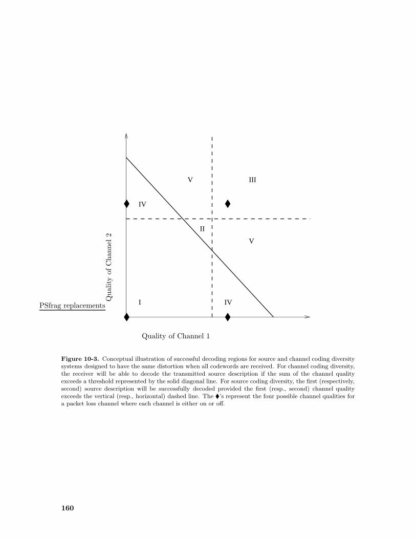
IV

II

I IV

III

V

V

PSfrag replacements

��

��

Quality of Channel 1

Quality

ofC

hannel

2

Figure 10-3. Conceptual illustration of successful decoding regions for source and channel coding diversitysystems designed to have the same distortion when all codewords are received. For channel coding diversity,the receiver will be able to decode the transmitted source description if the sum of the channel qualityexceeds a threshold represented by the solid diagonal line. For source coding diversity, the first (respectively,second) source description will be successfully decoded provided the first (resp., second) channel qualityexceeds the vertical (resp., horizontal) dashed line. The �’s represent the four possible channel qualities fora packet loss channel where each channel is either on or off.

160

for various systems. We refer to the slope of the distortion versus SNR on a log-log plotas the “distortion exponent” and use this as our figure of merit. In particular, our analysis

shows that optimal channel coding diversity is generally superior to source coding diversityon continuous channels in the sense that an optimal channel coding diversity architectureachieves a better distortion exponent than a source coding diversity architecture.

Since source coding diversity is best for on-off channels, and optimal channel codingdiversity is best for continuous state channels, our second question of whether there existsan architecture that combines the advantages of both becomes relevant. In addition to

our analysis of the two previously known diversity architectures in Fig. 10-2, our secondmain contribution is the description of a new joint source-channel decoding architecture

which achieves the best qualities of both. Specifically, to perform well on both continuousstate channels and on-off channels we do not propose a third encoding architecture, buta third new joint decoding architecture. We show that the main inefficiency of source

coding diversity on continuous state channels results from the channel decoders ignoringthe correlation between the multiple descriptions. By explicitly accounting for the structure

of the source encoding when performing channel decoding, we prove a coding theoremcharacterizing the performance of source coding diversity with joint decoding. We showthat such a system can achieve the same performance as optimal channel coding diversity

on continuous channels and the same performance as source coding diversity for on-offchannels.

� 10.1.1 Related Research

The problem of MD coding was initially studied from a rate-distortion perspective, havingbeen formalized by Gersho, Witsenhausen, Wolf, Wyner, Ziv, and Ozarow at the 1979IEEE Information Theory Workshop. Their initial contributions to the problem appear in

[183,185,140,184]. El Gamal & Cover develop an achievable rate region for two descriptionsin [71], and this region is shown to be optimal for the Gaussian source, with mean-square

distortion, by Ozarow [140]. Specialized results for the binary symmetric source, withHamming distortion, are developed by Berger & Zhang [20, 201, 202] and Ahlswede [3].Zamir [194] develops high-rate bounds for memoryless sources. Most recently, work by

Venkatarami et. al [174, 173] provides achievable rate regions for many descriptions thatgeneralize the results in [71, 201]. Important special cases of the MD coding problem have

also been examined, including successive refinement, or layered coding, [57,156] and certainsymmetric cases [147,148].

Some practical approaches to MD coding include MD scalar quantization, dithered MD

lattice quantization, and MD transform coding. Vaishampayan [172] pioneered the former,Frank-Dayan and Zamir considered the use of dither [68], and Wang, Orchard, Vaisham-

payan, and Reibman [180] and later Goyal & Kovacevic [76] studied the latter. See [75]for a thorough review of both approaches. Recently, the design of MD video coders hasreceived considerable attention [9, 10,154,91,167,179]

All of the classical work on MD coding utilizes an “on-off” model for the channels ornetworks under consideration, without imposing strict delay constraints. More specifically,source codes are designed assuming that each description is completely available (error-

free) at the receiver, or otherwise completely lost. Furthermore, the likelihood of theseevents occurring is independent of the choice of source coding rates. Under such conditions,

it is not surprising that MD coding outperforms SD coding; however, for many practicalchannel and network environments, these conditions do not hold. For example, in delay

161

constrained situations, suitable for real-time or interactive communication, descriptions mayhave to be encoded as multiple packets, each of which might be received or lost individually.

Furthermore, congestion and outage conditions often depend heavily upon the transmissionrate. Thus, it is important to consider MD coding over more practical channel models, aswell as to fairly compare performance with SD coding.

Some scattered work is appearing in this area. Ephremides et. al [4] examine MD codingover a parallel queue channel, compare to SD coding, and show that MD coding offers

significant advantages under high traffic (congestion) situations. This essentially resultsbecause the MD packets are more compact than SD packets, and indicates the importance

of considering the influence of rate on congestion. Coward et. al [48, 47] examine MDcoding over several channel models, including memoryless symbol-erasure and symbol-errorchannels, as well as block fading channels. For strict delay constraints, they show that

MD outperforms SD; for longer delay constraints, allowing for more sophisticated channelcoding, they show that SD outperforms MD. Thus, the impact of delay constraints are

important. This chapter examines fading conditions similar to those in [48,47], but considersa wider variety of channel coding and decoding options, with an emphasis on architectural

considerations as well as performance.

� 10.1.2 Outline

We begin by summarizing our system model in Section 10.2. Section 10.3 studies on-offchannels, Section 10.4 treats continuous state channels, and Section 10.5 develops source

coding diversity with joint decoding. Many of the more detailed proofs are deferred toAppendices. Finally, Section 10.6 closes the chapter with some concluding remarks anddirections for further research.

� 10.2 System Model

Fig. 10-1 depicts the general system model we consider in this chapter. Our objective is to

design and evaluate methods for communicating a source signal s with small distortion overcertain channels with independent parallel components. In particular, focusing on memo-

ryless source models for simplicity of exposition, we consider non-ergodic channels modelsin which delay constraints or limited channel variations limit the effective blocklength atthe encoder. Of many possible examples, we focus on on-off channels and additive noise

channels with block fading. While cross-layer design is generally acknowledged to yieldsuperior performance to layered design, simultaneously optimizing all facets of a system is

usually too complex. Hence we consider various architectures based upon using a classicalsystem at one layer combined with an optimized system at another layer. In the remain-der of this section, after briefly introducing some notation, we summarize the source and

channel models, discuss architectural options for encoding and decoding, and review high-resolutions approximations for the various source coding algorithms employed throughout

the chapter.

� 10.2.1 Notation

Vectors and sequences are denoted in bold (e.g., x) with the ith element denoted as x [i].Random variables are denoted using the sans serif font (e.g., x) while random vectors

and sequences are denoted with bold sans serif (e.g., x). We denote mutual information,differential entropy, and expectation as I(x ; y), h(x), E[x ]. Calligraphic letters denote sets

162

(e.g., s ∈ S). When its argument is a set or alphabet, | · | denotes the cardinality of theargument. To simplify the discussion of architectures, we use the symbols ENC(·) and

DEC(·) to denote a generic encoder and decoder. To specialize this generic notation to oneof the architectures discussed in Section 10.2.4, we will employ subscripts representing therelevant system variables.

� 10.2.2 Source Model

We model the source as a sequence of independent and identically distributed (i.i.d.) samples

s [k]. For example, such a discrete-time source may be obtained from sampling a continuous-time, appropriately band-limited, white-noise random process. We denote the probabilitydensity for the discrete-time source sequence s [k] as

ps(s) =

K∏

k=1

ps(s [k]) . (10.1)

We assume that the process is such that the differential entropy, h(s), and second moment,E[s2], both exist and are finite.

To measure quality of the communication system, we employ a distortion measure be-tween the source signal s and its reconstruction s ∈ S. Specifically, given a per-letter

distortion measure d(s [k] , s [k]), we extend it additively to blocks of source samples, i.e.,

d(s, s) =

K∑

k=1

d(s [k] , s [k]) . (10.2)

We may characterize performance in terms of various statistics of the distortion, viewed asa random variable. In particular, we focus on the expected distortion

D = E [d(s, s)] . (10.3)

Throughout our development, we will emphasize squared-error distortion, for which d(s, s) =

(s − s)2; in this case, (10.3) is the mean-square distortion.

� 10.2.3 (Parallel) Channel Model

The channel depicted by Fig. 10-1 consists of two branches, each of which corresponds to anindependent channel with independent states. Specifically, a channel input block, x, consistsof two sub-blocks, x1 and x2, and the corresponding channel output block, y, consists of the

two sub-blocks, y1 and y2. The channel states are denoted by random variables θ1 and θ2,respectively. The channel law is the product of the two independent sub-channel laws:

py1,y2,θ1,θ2|x1,x2(y1,y2, θ1, θ2|x1,x2) = py,θ|x(y1, θ1|x1) · py,θ|x(y2, θ2|x2) =

pθ(θ1) · pθ(θ2)

nc∏

i=1

[py |x ,θ(y1[i]|x1[i], θ1) · py |x ,θ(y2[i]|x2[i], θ2)

]. (10.4)

For simplicity, we only consider channels for which the input distribution that maximizes the

mutual information is independent of the channel state. Throughout the chapter we considerthe case where both the transmitter and receiver know the channel state distribution pθ and

163

the channel law py |x , but only the receiver knows the realized channel states and channeloutputs.

To examine fundamental performance and compare between systems, we analyze random

coding over these non-ergodic channels using outage probability [142] as a performancemeasure. Briefly, because the mutual information I , corresponding to the supportabletransmission rate of the channel, is a function of the fading coefficients or other channel

uncertainty, it too is a random variable. For fixed transmission rate R (in nats/channeluse), the outage probability Pr [I < R] measures channel coding robustness to uncertainty

in the channel.

The structure of the channel coding and decoding affects the form of the outage probabil-

ity expression [142]. If coding is performed over only the first component channel, then theprobability of decoding failure is Pr [I (x1; y1) < R]. If repetition coding is performed across

the parallel channels, then a single message is encoded as x1 = x2 = x. With selection com-bining at the receiver, the probability of decoding failure is Pr {max[I (x; y1), I (x; y2)] < R};with optimal maximum-ratio combining at the receiver, the probability of decoding failure

is Pr {I (x; y1, y2) < R}. Finally, if optimal parallel channel coding is performed using apair of jointly-designed codebooks with x1 and x2 independent, the probability of decoding

failure is Pr [I (x1; y1) + I (x2; y2) < R].

� 10.2.4 Architectural Options

In this section, we specify some architectural options for encoding and decoding in thesource-channel diversity system depicted in Fig. 10-1.

Joint Source-Channel Diversity

In the most general setup, joint source-channel diversity consists of a pair of mappings(ENCx1,x2←s,DECs←y1,y2). The encoder ENCx1,x2←s maps a sequence of K source lettersinto N pairs of channel inputs; correspondingly, the decoder maps N pairs of channel

outputs into K reconstruction letters. The ratio N/K (sometimes referred to as the pro-cessing gain, excess bandwidth, or bandwidth expansion factor) is denoted with the symbol

β∆= N/K.1 Mathematically,

ENCx1,x2←s : SK −→ XN1 ×XN

2 (10.5)

DECs←y1,y2 : YN1 ×YN

2 −→ SK . (10.6)

If the image of ENCx1,x2←s, i.e., ENCx1,x2←s(SK), is finite, we define the rate of the codeas

R =ln |ENCx1,x2←s(SK)|

N, (10.7)

which has units of nats per parallel channel use.

Regarding the non-ergodic nature of the channels, we consider situations in which K islarge enough to average over source fluctuations, i.e., the source is ergodic, but N is not

large enough to average over channel variations, i.e., the channel is non-ergodic.

1The bandwidth expansion ratio in [96] (denoted by L) is defined slightly differently from β. Specifically,since [96] considers a complex source and Rayleigh fading Gaussian noise channel, L = 2β.

164

PSfrag replacements

s sm mx1

x2

y1

y2Encoder Encoder DecoderDecoderParallel ChannelChannelChannel

Source Source

Figure 10-4. Channel coding diversity.

Channel Coding Diversity

From one perspective, a natural way to exploit diversity in the channel is to employ repeti-

tion or more powerful channel codes applied to a single digital representation of the source.In such scenarios, Fig. 10-1 specializes to that shown in Fig. 10-4. Such channel codingdiversity consists of a source pair of encoder and decoder mappings (ENCm←s,DECs←m)

and a channel pair of encoder and decoder mappings (ENCx←m,DECm←y). As in classicalrate-distortion source coding, the source encoder maps a sequence of K input letters to a

finite index, and the source decoder maps an index into a sequence of K reconstructionletters:

ENCm←s : SK −→ {1, 2, . . . , |M|} (10.8)

DECs←m : {0, 1, 2, . . . , |M|} −→ SK (10.9)

Further, as in classical channel coding, the channel encoder maps an index into N pairs of

channel inputs, and the channel decoder maps N pairs of channel outputs into an index:

ENCx←m : {1, 2, . . . , |M|} −→ XN1 × XN

2 (10.10)

DECm←y : YN1 × YN

2 −→ {0, 1, . . . , |M|} . (10.11)

Note that we include the index 0 at the output of the channel decoder and input to the

source decoder. This serves as a flag in the event of a (detected) channel coding error.

For the channel coding diversity approach, a key parameter is the rate defined by

R =ln |M|

N, (10.12)

where again the units are nats per parallel channel use.

Source Coding Diversity

Instead of exploiting diversity through channel coding, an emerging class of source codingalgorithms based upon MD coding allows diversity to be exploited by the source coding

layer.

For such source coding diversity, the block diagram of Fig. 10-1 specializes to that shown

in Fig. 10-5. Source coding diversity employs two independent, but otherwise classical,channel encoder and decoder pairs (ENCx1←m1,DECm1←y1

) and (ENCx2←m2,DECm2←y2):

ENCxi←mi : {1, 2, . . . , |Mi|} −→ XNi (10.13)

DECmi←yi: YN

i −→ {0, 1, 2, . . . , |Mi|} , (10.14)

for i = 1, 2. Again, we allow for the output of the channel decoding process to be 0 to

165

PSfrag replacements

s sm1 m1

m2 m2

x1

x2

y1

y2

Encoder

Encoder

Encoder

Decoder

Decoder

Decoder

Parallel

Channel

Channel

Channel

Channel

ChannelSourceSource

Figure 10-5. Source coding diversity system model described more precisely in Section 10.2.4.

m1 m2 DECs←m

= 0 = 0 DECs∅←m∅

= 0 6= 0 DECs1←m1

6= 0 = 0 DECs2←m2

6= 0 6= 0 DECs1,2←m1,2

Table 10.1. Source coding diversity decoder rules based upon channel conditions.

indicated a (detected) error. Here the rates

Ri =ln |Mi|

N, i = 1, 2 , (10.15)

both in nats per parallel channel use, are key parameters of the system.

The source encoder consists of two mappings

ENCmi←s : SK −→ {1, 2, . . . , |Mi|} , i = 1, 2 . (10.16)

The source decoder can be viewed as four separate mappings, depending upon whether or

not there are channel decoding errors on the individual channels. Specifically, the sourcedecoder can be constructed from the following four mappings:

DECs∅←m∅: {0} × {0} −→ {s∗}K (10.17)

DECs1←m1: {1, 2, . . . , |M1|} × {0} −→ SK

1 (10.18)

DECs2←m2 : {0} × {1, 2, . . . , |M2|} −→ SK2 (10.19)

DECs1,2←m1,2: {1, 2, . . . , |M1|} × {1, 2, . . . , |M2|} −→ SK

0 , (10.20)

where s∗ is a constant determined by the distortion measure for the source; for example,if mean-square distortion is important, then s∗ = E [s]. Table 10.1 summarizes how thesemappings are employed.

Source Coding Diversity with Joint Decoding

Finally, we also consider source coding diversity with joint decoding, as depicted in Fig. 10-6.

Here all is the same as in the source coding diversity model of Fig. 10-5, except that sourceand channel decoding is performed jointly across channels by accounting for correlationamong the channel coding inputs m1 and m2. Specifically, the channel decoding for this

approach is a mapping

DECm1,2←y1,2: YN

1 × YN2 −→ {0, 1, 2, . . . , |M1|} × {0, 1, 2, . . . , |M1|} (10.21)

166

PSfrag replacements

s sm1

m1

m2

m2

x1

x2

y1

y2

Encoder

Encoder

Encoder DecoderParallel

Channel

Channel

Channel ChannelSource Source

Figure 10-6. Source coding diversity with joint source-channel decoding.

which also takes into account knowledge of the source coding structure. In practice fulljoint-design of the decoder may not be required and a partially separated design wherelikelihood-ratios, quantized likelihood-ratios or similar information are exchanged between

the source and channel decoders may be sufficient.

� 10.2.5 High-Resolution Approximations for Source Coding

An important practical example of our source model is the Gaussian source, for which

ps(s) is a Gaussian density function with zero mean and unit variance. The Gaussiansource also serves as a useful approximation to other sources in the high resolution (low

distortion) regime [109, 194]. We now summarize the well-known results for single- andmultiple-description source coding for the Gaussian case, and generalize them using the high

resolution distortion approximations. These high resolution approximations are utilizedthroughout the sequel in our performance analysis.

Single Description Source Coding

In SD source coding, or classical rate-distortion theory, the source, s, is quantized into a

single description, s, using rate R.

In general, the rate-distortion function is difficult to determine, but a number of re-searchers have determined the rate-distortion function in the high resolution limit. Specifi-

cally, under some mild technical conditions [109],

limD→0

R(D)− 1

2log

e2h(s)

2πeD= 0 . (10.22)

This result also implies that2

R(D) ≈ 1

2log

e2h(s)

2πeD(10.23)

Without loss of generality we scale a given source under consideration so that e2h(s) = 2πe

to simplify the notation. Furthermore, instead of measuring the quantization rate in bits,we will find it more convenient to measure the rate in nats per channel sample by using the

processing gain β defined in Section 10.2.4. Thus we will use the expressions

R(D) ≈ 1

2βln

1

Dand exp R(D) ≈ D−1/(2β) (10.24)

2Throughout the chapter, the approximation f (x) ≈ g(x) is in the sense that f (x)/g(x) → 1 and|f (x) − g(x)| → 0 as x approaches a limit, either x → 0 or x → ∞, which should be clear from thecontext.

167

to approximate R(D) and exp R(D) in high-resolution.

As is well-known, the rate (in nats/channel sample) required for SD source coding of aGaussian source at average distortion D for any resolution is [46]

Rsd(D) =1

2βlog

1

D. (10.25)

Therefore, one way to interpret (10.23), is that for difference distortion measures in thehigh-resolution limit all sources essentially look Gaussian except for scaling by the constantfactor exp[2h(s)]/(2πe). Note that the form of the rate-distortion function in (10.23) is

asymptotically accurate and not a worst case result like those in [100,159].

Multiple Description Source Coding

In contrast to SD coding, MD source coding quantizes the source into two descriptions,

s1 and s2 so that if only one is received then moderate distortion is incurred, and if bothdescriptions are received then lower distortion is obtained [71].

The rates and distortions achievable by coding a unit variance Gaussian source intotwo equal-rate descriptions with a total rate of Rmd nats per channel sample, (i.e., each

description requires Rmd/2 nats) satisfy [71]

Rmd(D0,D1) =1

2βlog

1

D0+

1

2βlog

(1−D0)2

(1−D0)2 − (1− 2D1 + D0)2, (10.26a)

in the case of low distortions (2D1−D0 ≤ 1) where D0 is the distortion when both descrip-tions are received and D1 is the description when only a single description is received. Forhigh distortions with (2D1−D0 ≥ 1), there is no penalty for the multiple descriptions and

the total rate required is

Rmd(D0,D1) =1

2βlog

1

D0. (10.26b)

The general rate-distortion region for the MD coding problem is still unknown, in theGaussian case for more than two descriptions, and for more general sources. In the high

resolution limit the rate-distortion region is the same as for a Gaussian source with varianceexp[2h(s)]/(2πe) [194]. Hence for our asymptotic analysis we use the rate distortion function

in (10.26) for both Gaussian and non-Gausian sources with exp[2h(s)]/(2πe) = 1.

Exponentiating (10.26a) yields

exp[Rmd(D0,D1)] = D−1/(2β)0 · (1−D0)

−1/β

· (1− 2D0 + D20 − 1−D2

0 − 2D0 + 4D1 + 4D0D1 − 4D21)−1/(2β)

(10.27)

= D−1/(2β)0 · (1−D0)

−1/(β) · (4D1 − 4D0 + 4D0D1 − 4D21)−1/(2β)

(10.28)

≈ D−1/(2β)0 · (4D1 − 4D0)

−1/(2β) (10.29)

where the last line follows since (1−D0) ≈ 1 and 4(D1 −D0 + D0D1 −D21) ≈ 4(D1 −D0)

as D0 → 0 and D1 → 0. If only D0 → 0, then the ≈ in (10.29) must be replaced with '.

Any reasonable multiple description system has D0 ≤ D1/2 (otherwise the denominator of(10.26a) could be easily increased while decreasing the distortion by setting D1 = 2D0). So

168

since 2D1 ≤ 4(D1 −D0) ≤ 4D1 we obtain

(4D0D1)−1/(2β) / exp[Rmd(D0,D1)] / (2D0D1)

−1/(2β) (10.30)

where the lower bound holds when D0 → 0 and the upper bound also requires D1 → 0.

� 10.3 On-Off Component Channels

In this section, we examine the performance of source and channel coding diversity for

scenarios in which each of the component channels is either “on”, supporting a given trans-mission rate, or “off”, supporting no rate (or an arbitrarily small rate). Much of the

literature suggests that source coding diversity was developed for, and performs well on,such channel models. Our analysis is based upon channels that are parameterized in a

manner similar to the continuous channels in Section 10.4. This parameterization allows usto compare source and channel coding diversity over a broad range of operating conditions.In addition to confirming that there exist operating conditions for which source coding di-

versity significantly outperforms channel coding diversity, our results illustrate that therealso exist operating conditions for which the performance difference between source and

channel coding diversity is negligible.

� 10.3.1 Component Channel Model

For cases in which we are concerned with prolonged, deep fading or shadowing in a mo-bile radio channel, strong first-adjacent interference in a terrestrial broadcast channel, or

congestion in a network, we can model the channel state θi as taking on only two possiblevalues. Specifically, we can consider on-off channels where the channel mutual information

has probability law

I =

{

ln(1 + SNR) , with probability (1− ε)

0 , with probability ε. (10.31)

In (10.31), SNR parameterizes the channel quality when the channel is on, and ε parame-

terizes the probability that the channel is off. There is no connection between the channels’probability of being off and the quality in the on state; that is, neither SNR nor the selectedencoding rate R effects ε. By contrast, for the continuous channels discussed in Section 10.4,

ε will depend directly on both.

For simplicity of exposition, and ease of comparison with continuous channel scenarios

in the sequel, the term outage will refer to the inability of a given approach to conveyinformation over the pair of component channels. If both channels are off, then the systemexperiences outage regardless of the communication approach; however, as we will see,

different approaches may or may not experience outage when one of the channels is onand the other is off. For all of the approaches we discuss, due to the nature of the on-off

channels, performance can be classified into two regimes. The quality-limited regime hasaverage distortion performance varying dramatically with the channel quality in the on state,because the distortion under no outage dominates the average distortion. In this case, the

distortion under no outage is limited by the rate communicated, which, in turn, is limitedby the channel quality. The outage-limited regime has average distortion performance that

does not vary dramatically with the channel quality in the on state, because the distortionunder outage dominates the average distortion.

169

� 10.3.2 No Diversity

Combining a SD source coder with a single component channel with channel encoder anddecoder, the average distortion, as a function of the source coding rate R, is given by

E [DNO−DIV(R)] =

{

(1− ε) exp(−2β) + ε , if 0 < R ≤ ln(1 + SNR)

1 , otherwise. (10.32)

Thus, the minimum average distortion is

DNO−DIV = minR

E [DNO−DIV(R)]

= (1− ε)(1 + SNR)−2β + ε . (10.33)

We say that this system operates in the quality-limited regime if

(1 + SNR)2β � 1− ε

ε, (10.34)

in which case, the average distortion behaves essentially as (1− ε)(1 + SNR)−2β. If

(1 + SNR)2β � 1− ε

ε, (10.35)

the system operates in the outage-limited regime, in which case the average distortionbehaves essentially as ε.

� 10.3.3 Optimal Channel Coding Diversity

Combining a SD source coder with optimal parallel channel coding over the componentchannels, the average distortion, as a function of the source coding rate R, is given by

E [DOPT−CCDIV(R)] =

(1− ε2) exp(−2βR) + ε2 , if 0 < R ≤ ln(1 + SNR/2)

(1− ε)2 exp(−2βR) + [2ε− ε2] ,if ln

(1 + SNR

2

)< R

and R ≤ 2 ln(1 + SNR

2

)

1 , otherwise

.

(10.36)

For parallel channel coding, the two channel codewords are independent, and the system isable to sum the mutual informations of the component channels. This leads to the upperbound of R ≤ 2 ln(1+SNR/2) in the second case of (10.36). If we instead utilized repetition

coding, so that the two channel codewords are identical, the upper bound in the second casewould instead be R ≤ ln(1 + SNR).

In contrast to the case of no diversity, the performance of the optimal channel codingdiversity exhibits a discontinuity as a function of R. Fig. 10-7 illustrates that, becauseof the discrete probability distribution on the channel states, a discontinuity arises in the

outage probability about the point R = ln(1 + SNR/2).

Clearly, each case in (10.36) is minimized by utilizing the largest possible rate for that

170

Large Multiplexing Gain

Large Diversity Gain

PSfrag replacements

�

�

�

� I (x1; y1)

I (x2; y2)

Figure 10-7. Outage region boundaries for optimal parallel channel coding. The � symbols correspond tothe sample mutual information pairs (0, 0), (0, ln(1+SNR/2)), (ln(1+SNR/2), 0), and (ln(1+SNR/2), ln(1+SNR/2)). The solid line corresponds to the first case of (10.36), in which a low rate is selected to takeadvatange of diversity gain. The dashed line corresponds to the second case of (10.36), in which a higherrate is selected to take advantage of multiplexing gain. Outage regions are below and to the left of thesediagonals.

case. Then the minimum average distortion becomes

DOPT−CCDIV = minR

E [DOPT−CCDIV(R)]

= min{

(1− ε2)(1 + SNR/2)−2β + ε2 ,

(1− ε)2(1 + SNR/2)−4β + [1− (1− ε)2]}

. (10.37)

As Fig. 10-8 illustrates, the two terms in (10.37) have their own quality- and outage-limitedregimes, which, when combined by the minimum operation, leads to four trends in theoverall system performance.

Comparing the two terms in (10.37), we see that the different choices of rate lead to

different costs and benefits. Using the lower transmission rate, R = ln(1 + SNR/2), (cf.the first term in (10.37)) results in better outage-limited performance, but worse quality-limited performance. This approach exploits the diversity gain of the underlying parallel

channel. On the other hand, using the higher transmission rate, R = 2 ln(1 + SNR/2),(cf. the second term in (10.37)) results in worse outage-limited performance, but better

quality-limited performance. This approach exploits the multiplexing gain of the underlyingparallel channel. We note that the diversity and multiplexing terminology is inspired bythe inherent tradeoff between the two for multiple-input, multiple-output (MIMO) wireless

systems operating over fading channels [204].

Note that the two terms in (10.37) are equal when

(1 + SNR/2)2β =1− ε

2ε. (10.38)

171

0 10 20 30 40 50 60−60

−50

−40

−30

−20

−10

0

SNR (dB)

Ave

rage

Dis

tort

ion

(dB

)

Multiplexing, Quality−Limited

Diversity, Quality−Limited

Multiplexing, Outage−Limited

Diversity,Outage−Limited

Figure 10-8. Average distortion performance with ε = 10−2 for the first (solid line) and second (dashedline) terms in the minimization of (10.37).

For small SNR (such that (1+SNR/2)2β < (1− ε)/(2ε)), we exploit the multiplexing modeof operation and pass through its quality-limited and outage-limited regimes as we increaseSNR until (10.38) is satisfied. As we will see, passing through the outage-limited regime of

the multiplexing mode is the key limitation of optimal channel coding diversity for on-offchannels. For higher SNR (such that (1+SNR/2)2β > (1−ε)/(2ε)), we exploit the diversity

mode of operation and pass through its quality- and outage-limited regimes as we increaseSNR.

� 10.3.4 Source Coding Diversity

In this section, we approximate the minimum average distortion for an MD system with

independent channel coding. The analysis of this system is slightly more involved than thoseof previous sections because the rate-distortion region for MD coding is more complex, andindependent channel coding over on-off component channels involves a pair of outage events.

Similar to Fig. 10-7, Fig. 10-9 displays outage region boundaries for independent channel

coding. It is straightforward to see that the source coder should employ rates no greaterthan ln(1 + SNR/2) on each of the component channels; otherwise, one of the channelsexhibits outage with probability one, and the system can perform no better than the case

of no diversity with half the SNR. As a result, our analysis only considers the case Ri ≤ln(1+SNR/2). Moreover, due to the symmetry of the component channels, one can expect

symmetric rates, i.e., R1 = R2 = R, to be optimal; thus, we focus on this case. With thesesimplifications, we observe that, in contrast to the triangular outage regions for optimal

parallel channel coding in Fig. 10-7, the rectangular outage regions for independent channelcoding in Fig. 10-9 are well-matched to the on-off channel realizations.

Optimizing average distortion for the MD system requires a tradeoff between the dis-tortion D1 = D2 achieved when only one description is received and the joint distortion D0

achieved when both descriptions are received. Although this tradeoff is available in (10.30),we refactor it for our purposes here. Specifically, we set

D1 = D2 ≈{

exp(−(1− λ)2βR) , 0 ≤ λ < 1

1 , λ = 1, (10.39)

172

PSfrag replacements

�

�

�

�

I (x1; y1)

I (x2; y2)

Figure 10-9. Outage region boundaries for MD source coding with independent channel coding. The �symbols correspond to the sample mutual information pairs (0, 0), (0, ln(1 + SNR/2)), (ln(1 + SNR/2), 0),and (ln(1 + SNR/2), ln(1 + SNR/2)). The solid line corresponds to the outage region boundary for the firstchannel, and the dashed line corresponds to the outage region boundary for the second channel. The outageregion for channel one (resp. channel two) is to the left (resp. below) the boundary.

where R is the channel coding rate for a single channel. Thus, if λ = 0, the individual de-

scriptions achieve the single description rate-distortion bound. With this parameterizationof D1 and D2, the MD high-resolution approximation (10.30) yields

D0 ≈{

12 exp(−(1 + λ)2βR) , 0 ≤ λ < 1

exp(−4βR) , λ = 1(10.40)

for the joint distortion when both descriptions are received. We note that an essentially

identical approximation is developed in [76].The minimum average distortion for source coding diversity is then approximately

DSCDIV ≈ min{ min0<λ<1

ε2 + 2ε(1− ε)(1 + SNR/2)−(1−λ)2β +1

2(1− ε)2(1 + SNR/2)−(1+λ)2β,

[1− (1− ε)2] + (1− ε)2(1 + SNR/2)−4β} . (10.41)

For λ = 1, source coding diversity performance reduces to that of channel coding diversity;for λ = 0, source coding diversity performance reduces to that of no diversity with halfthe SNR. Because optimization over λ does not lend much insight, we delay discussion of

source coding diversity quality- and outage-limited regimes to the next section, where wealso compare with the other approaches.

� 10.3.5 Comparison

Fig. 10-10 compares average distortion performance of source and channel coding diversityby displaying the minimum average distortions (10.33), (10.37), and (10.41) as functions of

the component channel quality, SNR, in the on state, for different values of the probabilityof a component channel being off, ε. The results in Fig. 10-10 are clearly consistent with our

173

0 20 40 60−60

−50

−40

−30

−20

−10

0

SNR (dB)

Ave

rage

Dis

tort

ion

(dB

)

ε=10−4

0 20 40 60−60

−50

−40

−30

−20

−10

0

SNR (dB)

Ave

rage

Dis

tort

ion

(dB

)

ε=10−3

0 20 40 60−60

−50

−40

−30

−20

−10

0

SNR (dB)

Ave

rage

Dis

tort

ion

(dB

)

ε=10−2

0 20 40 60−60

−50

−40

−30

−20

−10

0

SNR (dB)

Ave

rage

Dis

tort

ion

(dB

)

ε=10−1

Figure 10-10. Average distortion performance over on-off channels. The plots show average distortion as afunction of SNR; successively lower curves correspond to no diversity (dotted lines), optimal channel codingdiversity (dashed lines), and source coding diversity (solid lines), respectively. Each plot corresponds to adifferent value for the probability ε of a component channel being off, and all are for β = 1.

174

intuitive discussion of source and channel coding diversity performance in Section 10.1.1.For moderate SNR, depending upon ε, both systems exhibit transitions from SNR−4 be-

havior to SNR−2 behavior; however, the transition is generally less drastic for source codingdiversity, especially for smaller ε. The difference between the two systems is apparently theoutage-limited behavior of the multiplexing mode for optimal channel coding diversity, for

which the outage regions are not well-matched to the channel realizations. By contrast,the transition between the two quality-limited trends for source coding diversity is much

less drastic, and this graceful degradation property of source coding diversity leads to theirbetter performance over on-off channels. However, it is important to note that there isnegligible difference between optimal channel coding diversity and source coding diversity

at both low and high SNR.

� 10.4 Continuous State Channels

In cases where we are concerned with time or frequency selective multipath fading in amobile radio channel or a range of possible interference levels in a cellular network, we canmodel the channel state θi as taking on a continuum of values. For example, multiplicative

fading is commonly modeled as a Rayleigh or Nakagami random variable in such scenarios.In the following section we study the average mean square distortion in the limit of high

SNR for such continuous channels when the channel state is known to the receiver but notthe transmitter. Since the distortion generally behaves as SNR−∆ for such channels, we aremainly interested in computing the distortion exponent defined as

∆ = − limSNR→∞

log E[D]

log SNR. (10.42)

Note that there is an important difference between the average or transmit signal-to-noise ratio which is deterministic and known by both transmitter and receiver and the

instantaneous or block signal-to-noise ratio which is random and known only at the receiver.Throughout the rest of the chapter, we always use SNR to refer to the former and consider

the random, instantaneous signal-to-noise ratio as a random variable.

In Section 10.4.7, we plot the distortion exponents as well as the numerically com-

puted average distortions for a Gaussian source transmitted over a complex Rayleigh fadingadditive white Gaussian noise channel. Hence the reader may find it useful to refer toFigures 10-11 and 10-12 as a concrete example for comparing the following results for the

performance of each system.

� 10.4.1 Continuous Channel Model

For continuous state channels, the distribution of the mutual information random variable isgenerally difficult to compute exactly. For complex, additive white Gaussian noise channels

with multiplicative fading, however, the mutual information random variable is I = log(1+θ · SNR) where θ corresponds to the multiplicative fading which is normalized so thatE[θ] = 1 so that SNR is the transmit power or equivalently, the average received power.

For θ · SNR� 1, we have

I = log(θ · SNR) + log

(

1 +1

θ · SNR

)

= log(θ · SNR) + O

(1

θ · SNR

)

≈ log(θ · SNR)

175

and so exp I is close to SNR · θ. 3 Thus, for additive Gaussian noise channels with mul-tiplicative fading, we can develop asymptotic results by considering the first terms in the

Taylor series expansion of the distribution of θ near zero. More generally, we can focus onthe high SNR limit by considering the Taylor series expansion of the distribution for themutual information random variable for each channel.

Specifically, let fI (t) and FI (t) represent the probability density function (PDF) andcumulative distribution function (CDF) for the mutual information and let feI (t) and FeI (t)

represent the PDF and CDF for I .4 We consider the case where there exists a parametercalled SNR such that

feI (t) ≈ cp

(t

SNR

)p−1

(with p ≥ 1) (10.43)

and consequently FeI (t) can be approximated via

FeI (t) ≈ c

(t

SNR

)p

. (10.44)

Intuitively, SNR represents the transmit signal-to-noise ratio or the average signal-to-noiseratio and FeI (t) is the probability that the instantaneous signal-to-noise ratio is below t. As

introduced in Section 10.2.5, the notion of approximation we use is that a(SNR) ≈ b(SNR)if limSNR→∞ a(SNR)/b(SNR) = 1 and limSNR→∞ |a(SNR)− b(SNR)| = 0.

For example, in wireless communications, a common model is an additive white Gaussian

noise channel with fading:y [i] = θ · x [i] + z [i] (10.45)

where θ represents the fading and z [i] represents additive noise. A common approach is to

obtain robustness by coding over two separate frequency bands or time-slots in which casethe channel model becomes

y1[i] = θ1 · x1[i] + z1[i]

y2[i] = θ2 · x2[i] + z2[i].

If we are interested in Rayleigh fading then each θi has an exponential distribution and athigh SNR, the cumulative distribution function for exp I (yi; xi) is approximated by t/SNRand hence the parameters c and p in (10.44) are both unity (e.g., see [98,181] for a discussion

of such high SNR expansions).

� 10.4.2 No Diversity

Perhaps the simplest case to consider is when there is only a single channel and no diversity is

present. For such a scenario, a natural approach is cascading an SD source encoder/decoderENCm←s(·)/DECs←m(·) with a single channel encoder/decoder ENCx←m(·)/DECm←y(·). In

terms of our general joint source-channel coding notation such a system has the encoder

3A similar expression can also be obtained for additive noise channels with non-Gaussian noise (e.g.,using techniques from [196, 118]).

4Recall that we assume the mutual information optimizing input distribution is independent of the channelstate. Hence it makes sense to speak of the mutual information distribution as given instead of a parametercontrolled by the system designer.

176

and decoder

x = ENCx←s(s) = ENCx←m(ENCm←s(s)) (10.46a)

s = DECs←y(y) =

{

DECs←m(DECm←y(y)), DECm←y(y) 6= 0

E[s], otherwise.(10.46b)

Theorem 34. The distortion exponent for a system with no diversity described by (10.46)is

∆NO−DIV =2βp

2β + p, (10.47)

where β is the processing gain defined in Section 10.2.4 and p is the diversity order of thechannel approximation in (10.44).

Proof. The average distortion is

E[D] = minD

Pr[I (x ; y) < R(D)] + {1− Pr[I (x ; y) < R(D)]} ·D (10.48)

= minD

FeI (exp R(D)) + [1− FeI (R(D))] ·D (10.49)

≈ minD

cD−p/(2β)

SNRp +

[

1− cD−p/(2β)

SNRp

]

·D (10.50)

≈ minD

cD−p/(2β)

SNRp + D. (10.51)

Differentiating and setting equal to 0 yields the minimizing distortion

D∗ =

(2β

cp

) −2β2β+p

· SNR−2βp2β+p .

Substituting this into (10.51) yields

E[D] ≈ CNO−DIV · SNR−2βp2β+p . (10.52)

where CNO−DIV represents a term independent of SNR. Thus the distortion exponent is

2βp/(2β + p).

� 10.4.3 Selection Channel Coding Diversity

Perhaps the simplest approach to using two independent channels is to use SD sourcecoding with repetition channel coding and selection combining. In this scheme, the encoder

quantizes the source, s, to s, adds channel coding to produce x, and repeats the resulton both channels. The receiver decodes the higher quality channel and ignores the other.Formally, the encoder and decoder are given by

(x1, x2) = ENCx1,x2←s(s) = (ENCx←m(ENCm←s(s)),ENCx←m(ENCm←s(s))) (10.53a)

s = DECs←y1,y2(y1, y2) =

DECs←m(DECm←y(y1)), DECm←y(y1) 6= 0

DECs←m(DECm←y(y2)),DECm←y(y1) = 0and DECm←y(y2) 6= 0

E[s], otherwise

(10.53b)

177

where the SD source encoder/decoder and the single channel encoder/decoder are denoted

ENCm←s(·)/DECs←m(·) and ENCx←m(·)/DECm←y(·).

Thus, the quantized source signal will be recovered provided either channel is good. While

such a scheme is sub-optimal in terms of resource use, it is simplest to understand and easiestto implement. The following theorem (proved in Appendix H.1) characterize asymptoticperformance.

Theorem 35. The distortion exponent for a system with selection channel coding diversitydescribed by (10.53) is

∆SEL−CCDIV =2βp

β + p. (10.54)

� 10.4.4 Multiplexed Channel Coding Diversity

A key drawback of repetition coding with selection combining is that it wastes the poten-tial bandwidth of one channel in order to provide diversity. When the channel is usually

good, such a scheme can be significantly sub-optimal. Hence, a complementary approachis channel multiplexing where the source is quantized using SD coding and this message is

split over both channels. We define a channel multiplexing system as one with encoder anddecoder given by

(x1, x2) = ENCx1,x2←s(s) = (ENCx1←m1(ENCm1←s(s)),ENCx2←m2(ENCm2←s(s)))

(10.55a)

s = DECs←y1,y2(y1, y2) =

DECs←m(DECm1←y1(y1),DECm2←y2

(y2)), DECm1←y1(y1) 6= 0 and

DECm2←y2(y2) 6= 0

E[s], otherwise.

(10.55b)

where the single channel encoders/decoders, the first and second half of the output of asingle description source encoder, and the source decoder are denoted

ENCxi←mi(·)/DECmi←yi(·) and ENCmi←s(·) and DECs←m(·).

If both channels are good enough to support successful decoding, then this scheme can

transmit roughly twice the rate of a repetition coding system. The drawback is since eitherchannel being bad can cause decoding failure, the system is less robust. The following

theorem (proved in Appendix H.2) characterizes asymptotic performance.

Theorem 36. The distortion exponent for a system with multiplexed channel coding diver-

sity described by (10.55) is

∆MPX−CCDIV = 4pβ/(p + 4β). (10.56)

Intuitively, we expect that when bandwidth is plentiful and outage is the dominatingconcern, the diversity provided by repetition coding is more important than the extra rate

provided by channel multiplexing. When bandwidth is scarce, we expect the reverse to betrue. We can verify this intuition by examining the distortion exponents in these two limits

178

to obtain

limβ/p→∞

∆SEL−CCDIV

∆MPX−CCDIV= 2 (10.57)

limβ/p→0

∆SEL−CCDIV

∆MPX−CCDIV=

1

2. (10.58)

The distortion exponents are equal if p = 2β.

� 10.4.5 Optimal Channel Coding Diversity

Each of the previous schemes used SD source coding with some form of independent channelcoding and hence was sub-optimal. With SD source coding, the optimal strategy is to use

parallel channel coding. In this scheme, the two component channels are treated as asingle parallel channel with channel encoding and decoding performed jointly over both.

Specifically, we define optimal channel coding diversity as

(x1, x2) = ENCx1,x2←s(s) = ENCx←m(ENCm←s(s)) (10.59a)

s = DECs←y1,y2(y1, y2) =

{

DECs←m(DECm←y(y1, y2)), DECm←y(y1, y2) 6= 0

E[s], otherwise(10.59b)

where the SD source encoder/decoder and the parallel channel encoder/decoder are denoted

ENCm←s(·)/DECs←m(·) and ENCx←m(·)/DECm←y(·).

Since parallel channel coding optimally uses the channel resources, it dominates both rep-etition coding with selection combining and channel multiplexing as characterized by the

following theorem (proved in Appendix H.3).

Theorem 37. The distortion exponent for a system with optimal channel coding diversitydescribed by (10.59) is

∆OPT−CCDIV =4pβ

p + 2β. (10.60)

� 10.4.6 Source Coding Diversity

Next, we consider the case where the source is transmitted over a pair of independentchannels using MD source coding. Specifically, we consider a system with

(x1, x2) = ENCx1,x2←s(s) = (ENCx1←m1(ENCm1←s(s)),ENCx2←m2(ENCm2←s(s)))(10.61a)

179

s = DECs←y1,y2(y1, y2) =

DECs1←m1(DECm1←y1(y1)), DECm1←y1(y1) 6= 0 and

DECm2←y2(y2) = 0

DECs2←m2(DECm2←y2

(y2)), DECm1←y1(y1) = 0 and

DECm2←y2(y2) 6= 0

DECs1,2←m1,2(DECm1←y1

(y1),DECm2←y2(y2)), DECm1←y1

(y1) 6= 0 and

DECm2←y2(y2) 6= 0

E[s], DECm1←y1(y1) = 0 and

DECm2←y2(y2) = 0

(10.61b)

where ENCm1←s(·) and ENCm2←s(·) represent the two quantizations of the source pro-duced by the MD source coder, DECsi←mi

(·) represent the possible source decoders de-

scribed in Table 10.1, and ENCxi←mi(·) / DECmi←yi(·) correspond to single channel en-

coders/decoders. The performance of such a system is characterized by Theorem 38 (proved

in Appendix H.4).

Theorem 38. The distortion exponent for source coding diversity as described by (10.61)is

∆SCDIV = max

[8βp

4β + 3p,

4βp

4β + p

]

. (10.62)

When p ≤ 4β, MD source coding achieves diversity in the sense that if either channel is

bad but the other is good a coarse-grained description of the source can be reconstructedwhile if both channels are good, a fine-grained description can be reconstructed. There-fore, in this regime, source coding diversity dominates sub-optimal channel coding diversity

because it takes advantage of the redundancy between descriptions at the source codinglayer.

When p ≥ 4β, however, the max in (10.62) selects the second term. In this regime, itis more important to maximizes the transmitted rate than protect against fading. Thus

source coding diversity degenerates into multiplex channel coding diversity as analyzed inSection 10.4.4.

In both regimes, optimal channel coding diversity dominates source coding diversity.

� 10.4.7 Rayleigh Fading AWGN Example

In this section, we evaluate the various distortion exponents on a complex Rayleigh fadingadditive white Gaussian noise (AWGN) channel. The high SNR approximation for the

mutual information on each Rayleigh fading AWGN channel is FeI (t) ≈ (t/SNR), i.e.,p = 1 in (10.44) (e.g., see [98,181] for a discussion of such high SNR expansions).

The resulting distortion exponents are summarized5 in Table 10.2 and plotted in Fig. 10-11.When the processing gain is small (i.e., β � 1), multiplex and optimal channel coding di-versity as well as source coding diversity all approach a distortion exponent of 4β, while

selection channel coding diversity and no diversity both approach distortion exponents of2β. Intuitively, this occurs because since bandwidth is scarce, a good system should try to

maximize the information communicated by sending different information on each channel.

5The distortion exponents in this chapter are slightly different than in [96] due to different definitions ofthe processing gain as described in Section 10.2.4.

180

Multiplex coding does this by sending different information on each channel using the samecode, optimal channel coding does this by using a different code for each channel, and mul-

tiple descriptions coding does this by sending different source descriptions on each channel.Since neither selection diversity nor no diversity provide any multiplexing gain (in the senseof [204]) both of these systems achieve the same sub-optimal distortion exponent.

When the processing gain is large (i.e., β � 1), selection and optimal channel codingdiversity as well as source coding diversity all approach a distortion exponent of 2, while

systems with multiplex channel coding diversity or no diversity achieve a smaller distortionexponent of 1. Intuitively, this occurs because, since bandwidth is plentiful, even one good

channel provides plenty of rate to send a satisfactory description of the source. Thus goodsystems should try to maximize robustness by being able to decode even if one channel failscompletely.

At both extremes of processing gain, the best distortion exponent can be achieved either

by exploiting diversity at the physical layer via parallel channel coding or at the applicationlayer via multiple description coding. In some sense, this suggests that both physical layerand application layer systems are flexible enough to incorporate the main principles of

diversity for continuous channels. Other sub-optimal schemes such as selection channelcoding diversity are less flexible in that they only incorporate a subset of the important

principles of diversity and thus approach the best distortion exponent in at most one extremeof processing gain. For all processing gains, however, optimal channel coding diversity issuperior to source coding diversity, suggesting that the application layer system is missing

something. In Section 10.5, we show that the loss of source coding diversity is essentiallycaused by separating the process of channel decoding from source decoding.

Table 10.2. Distortion exponents.

System ∆

No Diversity (Section 10.4.2) 2β/(2β + 1)

Selection Channel Coding Diversity (Section 10.4.5) 2β/(β + 1)

Multiplex Channel Coding Diversity (Section 10.4.4) 4β/(4β + 1)

Optimal Channel Coding Diversity (Section 10.4.5) 4β/(2β + 1)

Source Coding Diversity (Section 10.4.6) max[8β/(4β + 3), 4β/(4β + 1)]

Fig. 10-12 shows the average distortion for various systems transmitting over complex

Rayleigh fading AWGN channels with β = 1 where the parameters in the rate optimizationshave been numerically computed for each system using the high SNR approximations. Asthe plot indicates, the difference in performance suggested by the asymptotic results in

Table 10.2 becomes evident even at reasonable SNR. Indeed, as the figure shows, optimalchannel coding diversity is always superior to source diversity and achieves an advantage of

a few dB at moderate SNR. Source diversity is superior to selection diversity by a similarmargin. In contrast, Fig. 10-10 shows that for on-off channels, source-diversity is alwaysbetter than optimal channel coding diversity for on-off channels. Evidently, none of the

systems considered so far are universally optimal and the best way to achieve diversitydepends on the qualitative features of the channel. In the next section, we consider a joint

source-channel coding system which we show achieves the benefits of source-diversity foron-off channels and the benefits of optimal channel diversity for continuous state channels.

181

Figure 10-11. Distortion exponents as a function of bandwidth expansion factor β in decibels. From topto bottom on the right hand side the curves correspond to optimal channel coding diversity (Section 10.4.5),source coding diversity (Section 10.4.6), selection channel coding diversity (Section 10.4.3), multiplexedchannel coding diversity (Section 10.4.4), and no diversity (Section 10.4.2).

−40

−30

−20

−10

0

Dis

tort

ion

(dB

)

0 10 20 30 40SNR (dB)

Figure 10-12. Average distortion performance on a complex Rayleigh fading additive white Gaussian noisechannel with processing gain β = 1. From top to bottom on the right hand side the curves correspond tono diversity (Section 10.4.2), multiplexed channel coding diversity (Section 10.4.4), selection channel codingdiversity (Section 10.4.3), source coding diversity (Section 10.4.6), and optimal channel coding diversity(Section 10.4.5).

182

� 10.5 Source Coding Diversity with Joint Decoding

In this section we consider source coding diversity with a joint decoder that uses the redun-dancy in both the source coder and channel coder to decode the received signal. Specifically,

we define source coding diversity with joint decoding to have encoder and decoder

(x1, x2) = ENCx1,x2←s(s) = (ENCx1←m1(ENCm1←s(s)),ENCx2←m2(ENCm2←s(s)))(10.63a)

s = DECs←y1,y2(y1, y2) (10.63b)

where ENCx1←m1(·)/ENCx1←m1(·) are single channel encoders (with potentially but not nec-

essarily different codes), ENCm1←s(·)/ENCm2←s(·) are MD source encoders, DECs←y1,y2(·)denotes a joint source-channel decoder to be described in the sequel.

The motivation for joint source-channel decoding is illustrated by considering the con-

ceptual diagram of an MD quantizer in Fig. 10-13. Since the two quantization indexesENCm1←s(s) and ENCm2←s(s) are correlated, the channel decoder should take this corre-

lation into account. For example, if one channel is good and y1 is accurately decoded tom1 = ENCm1←s(s) this decreases the number of possible values for m2 and makes decodingy2 easier.

PSfrag replacements s

m1

m2

Figure 10-13. Conceptual diagram of an MD quantizer. The source s is mapped to the quantizer binslabeled m1 = ENCm1←s(s) and m2 = ENCm2←s(s). Since only overlapping pairs of indexes are legalquantization values, if a receiver accurately decodes m1 from the channel output y1, then there are only twopossible values for m2 in decoding a second channel output y2.

We show that a joint decoder that exploits this correlation can enlarge the region whereboth m1 and m2 are successfully decoded. Specifically, with separate decoding, both de-

scriptions are decoded when both I (x1; y1) and I (x2; y2) exceed some rate threshold RT ,which is denoted as region III in Fig. 10-3. A joint decoder, however, also recovers bothdescriptions in region II yielding the decoding regions shown in Fig. 10-14. With these

enlarged decoding regions, we show that source coding diversity with joint source-channeldecoding achieves the same performance as optimal channel coding diversity for continuous

channels in addition to providing the benefits of source coding diversity for on-off channels.

� 10.5.1 System Description

Next we describe one way to implement the architecture in (10.63) using an informationtheoretic formulation and random coding arguments.

183

PSfrag replacements

Outage

Decode Both

m1 and m2

Decode m1

Dec

ode

m2

I (x1; y1)

I (x2; y2)

Figure 10-14. Decoding regions for a joint source-channel decoder.

Source Encoding

Choose a test-channel distribution ps1 ,s2|s(s1, s2|s) with the marginal distributions

psi(si) =∑

s,s3−i

ps1 ,s2|s(s1, s2|s)ps(s), for i ∈ {1, 2}. (10.64)

Create a pair of rate R random source codebooks, C1 and C2 by randomly generatingexp nsR sequences of length ns according to the i.i.d. test-channel distributions psi(si). To

encode a source, find a pair of codewords s1 ∈ C1, s2 ∈ C2, such that the triple (s1, s2, s) isstrongly typical. According to [71], encoding will succeed with probability approaching oneif6

R > I (s1; s) (10.65a)

R > I (s2; s) (10.65b)

2R > I(s; s1s2) + I (s1; s2). (10.65c)

Channel Encoding

For each channel, generate a rate R random codebook, Ci, by randomly selecting exp(nsR)

sequences (or equivalently exp(ncR/β) sequences) of length nc according to the i.i.d. dis-tribution px(x). Encode the source codeword in the ith row of Cj by mapping it to the ithchannel codeword in Cj .

Joint Decoding

Denote the output of channel j as yj for j ∈ {1, 2}. To decode, create the lists L1 and L2,by finding all channel codewords, xj ∈ Cj , such that the pair (xj, yj) is typical with respectto the distribution pyj ,xj |θj

(y, x|θj). Next search for a unique pair of codewords (x1, x2)

6Note that [71] also includes a term s0 which can be ignored (i.e., s0 can be set to null or set to a constantsuch as 0) for our purposes.

184

with x1 ∈ C1 and x2 ∈ C2 such that the corresponding source codewords (s1, s2) are typicalwith respect to the distribution ps1 ,s2(s1, s2). If a unique pair is found, output the resulting

source reconstructions. Otherwise declare a decoding error.

Probability Of Error

The following theorem provides an achievable rate for source coding diversity with jointdecoding.

Theorem 39. Joint decoding will succeed with probability approaching one if

max [0, R− β · I (x1; y1)] + max [0, R− β · I (x2; y2)] ≤ I (s1; s2). (10.66)

Proof. Decoding can fail if either the correct pair of source codewords are not typical or ifan incorrect pair of source codewords are typical. According to the law of large numbers

the probability of the former event tends to zero as the block length increases. Therefore,the union bound implies that if the probability of the latter tends to zero, then the totalprobability of a decoding error also tends to zero.

The probability that an incorrect pair of channel codewords is typical according topyj ,xj |θj

(y, x|θj) is roughly exp−ncI (xj ; yj). Since there are exp nsR possible codewords for

each channel, the expected list sizes are

|Lj | = 1 + exp [nsR− ncI (xj ; yj)] + ε (10.67)

where the “1” corresponds to the correct channel codeword and ε denotes a quantity whichgoes to 0. Using standard arguments it is possible to show that the actual list sizes will be

close to the expected list size with probability approaching one.

The probability that an incorrect pair of source codewords, (s1, s2) corresponding to the

channel codeword pair (x1, x2) with xj ∈ Cj is typical is roughly exp−nsI (s1; s2). Multiply-ing this probability by the number of incorrect pairs yields the expected number of incorrect

codewords which are nonetheless typical:

exp {−nsI (s1; s2) + max [0, nsR− ncI (x1; y1)] + max [0, nsR− ncI (x2; y2)]} . (10.68)

Therefore, after dividing through by ns and recalling that the processing gain is defined asβ = nc/ns, we conclude that decoding succeeds provided that (10.66) holds.

� 10.5.2 Performance

In order to analyze performance, we must first choose a distribution for the source and

channel codebooks. Naturally, we choose the capacity optimizing input distribution foreach channel codebook Cj . For the source codebook distribution we use a simpler form ofthe additive noise test-channel in [71]:

sj = s + nj (10.69)

where (n1, n2) is a pair of zero-mean, variance σ2, Gaussian random variables independentof s and each other. For this distribution, the distortion when using only description j is

Dj ≤ σ2. When both descriptions are received they can be averaged to yield distortionD1,2 ≤ σ2/2.

185

Performance on Continuous Channels

To derive the performance on continuous channels, we must choose σ2 as a function of thechannel parameters. The choice of σ2 determines the rate and hence also the probability of

outage and the distortion exponent. Our goal is to show that source coding diversity withjoint decoding achieves the same distortion exponent as optimal channel coding diversity.Hence instead of solving an optimization problem to determine σ2, we make an educated

guess inspired by (H.30) to choose7

σ2 = SNR−4pβp+2β

.(10.70)

Theorem 40. The distortion exponent for source coding diversity with joint decoding is atleast as good as that for optimal channel coding diversity:

∆SCDIV−JD ≥ ∆OPT−CCDIV . (10.71)

Note that to achieve the distortion exponent in the previous theorem, the multiple

description source redundancy is used in two qualitatively different ways. First, the re-dundnacy between x1 and x2 is used to recover the two source descriptions. In this sense,

the source coding redundancy acts like channel coding redundancy in providing robustnessto noise. Next, the redundancy between s1 and s2 is used to produce a better source recon-struction by averaging out the quantization noise. Thus, the benefit of joint source-channel

decoding is that it can gain the maximum benefit of the redundancy required by multipledescription coding both at the channel decoding stage and the source decoding stage.


We considered various architectures to minimize the average distortion in transmitting

a source over independent parallel channels. Conceptually, we view the overall channelquality encountered by a system as a two-dimensional random variable where the two axes

correspond to the Shannon mutual information for each channel. As illustrated in Fig. 10-3,the different architectures considered essentially correspond to systems which perform wellwhen the channel quality is in a certain part of this two-dimensional mutual information

plane. Thus minimizing the distortion for a given channel model corresponds to choosing anarchitecture matched to the shape of the overall channel mutual information distribution.

For on-off channel models, where a channel either fails completely or functions normally,the overall channel mutual information takes values on the Cartesian product of a finiteset. This shape is well matched to source coding diversity, i.e., MD source coding and

independent channel coding, that exploits diversity at the application layer. Specifically,in the high SNR regime, it is essential that both channels carry redundant information

so that if one channel fails the signal can still be decoded from the surviving channel.This forces channel coding diversity to use complete redundancy, and so the distortionwhen both channels are on is the same as when only one channel is on. In contrast, source

coding diversity can use only partial redundancy by sending slightly different signals on eachchannel. When both channels are on, the differences in the two received descriptions lead to

a higher resolution reconstruction and lower distortion. Therefore, source coding diversity

7 Technically, it would be better to choose σ2 to be proportional to the right hand side of (10.70) with acomplicated proportionality constant. Since distortion exponent analysis essentially ignores constant factors,however, we ignore this refinement to simplify the exposition.

186

achieves substantially better performance than channel coding diversity as illustrated inFig. 10-10.

In contrast, for fading, shadowing, and similar effects, the overall channel mutual infor-mation takes on a continuous range of values. This shape is better suited to optimal channelcoding diversity that exploits at the physical layer. Specifically, in the high SNR regime,

optimal channel coding diversity takes advantage of redundancy between the informationtransmitted across each channel while source coding diversity with separate decoding can-

not. As one of our main results, we showed that for such channels the average distortionasymptotically behaves as SNR−∆. In particular, we calculated the distortion exponent∆ for various architectures and showed that the distortion exponent for optimal channel

coding diversity is strictly better than for source coding diversity.Finally, we demonstrated that there is no inherent flaw in source coding diversity on

continuous channels. Instead, the inferior distortion exponent of source coding diversity isdue to the sub-optimality of separate source and channel decoding. If joint source-channeldecoding is allowed, source coding diversity achieves the same distortion exponent as optimal

channel coding diversity. Thus, for the non-ergodic channels considered in this chapter,Shannon’s source-channel separation theorem fails,8 and the best overall performance is

achieved by a joint source-channel architecture using multiple description coding.Essentially, the architectural implications of our results can be summarized as follows.

Application layer diversity is best for on-off channels, physical layer diversity is best for

continuous-state channels, and (of the limited schemes we considered) joint source-channelcoding achieves the best performance in either regime. Our results provide a way to balance

the cost of choosing a potentially sub-optimal architecture against other concerns such asimplementation complexity, ease of deployment, etc. Finally, our results on joint source-channel coding illustrate the price of layering incurred in separating source and channel

coding.While this chapter explores a variety of architectures, many aspects of the detailed

design, analysis and implementation of such systems remain to be addressed. On the in-formation theory side, determining the best possible average distortion, or at least lowerbounds to the best distortion, would be a valuable step. Similarly, determining the perfor-

mance for architectures using broadcast channel codes combined with successive refinementsource codes, hybrid digital-analog codes, or other joint source-channel architectures would

be interesting. Also, determining second-order performance metrics beyond the distortionexponent would be useful in designing practical systems. Some issues of interest in signalprocessing and communication theory include developing practical codes achieving the the-

oretical advantages of joint source-channel decoding, generalizing the results in this chapterto sources with memory or correlated channels (e.g., as found in multiple antenna systems),

and studying the effect of imperfect channel state information at the receiver. Finally, awide array of similar questions arise in a variety of network problems such as relay channels,multi-hop channels, and interference channels. For network scenarios, both the number of

possible architectures as well as the advantages of sophisticated systems will be larger.

8We believe that the main value of Shannon’s original source-channel separation theorem was in showingthat bits are a sufficient currency between source and channel coding systems. Thus even though the systemin Section 10.5 has separate encoding and only the decoding is performed jointly, we say that the separationtheorem breaks down because exchanging bits is no longer sufficient. Specifically, such a joint decodingsystem would need to pass lists, log-likelihood ratios, or similar information from the channel coding layerto the source coding layer.

187

188

Chapter 11

Concluding Remarks

189

� 11.1 Distortion Side Information Models

In the first part of this thesis we focused on dynamics in source coding. Essentially, ourgoal was to study scenarios where the relative importance or qualitative notion of distortion

varies throughout the source signal. To do so, we introduced the idea of side informationwhich affects the distortion measure but is independent of the source. We developed thetheory of such distortion side information and showed that knowing it at the encoder is

often as good as knowing it at both encoder and decoder. Furthermore, we constructedpractical algorithms to exploit such side information using lattices and erasure quantization

codes. If linear complexity erasure quantization codes (such as the ones in Chapter 4) areused, these constructions require only linear complexity to fully utilize the distortion sideinformation.

Our results about distortion side information illustrate a new principle for use in lossycompression. Specifically, in addition to the boundary gain achieved by entropy coding and

the granular gain achieved by choosing a good high-dimensional packing, distortion sideinformation provides a way to exploit the “modelling gain” of a more accurate distortion

measure. The fact that distortion side information based quantizers require only linearcomplexity suggests that this principle is one which can be practically implemented. Beyondthe specific results presented in this thesis, we believe that exploring the role of dynamic

distortion models may lead to a rich set of new possibilities for source coding.

First, while there is a growing understanding of perceptual effects in lossy compres-

sion, leveraging such knowledge can be difficult due to the complexity of incorporating itin classical quantizer design. In contrast, the framework presented in this thesis provides aclean interface between the tasks of constructing quantizers and investigating the proper-

ties of human perception. Biologists, psychologists, and cognitive scientists can debate andpropose distortion side information models while engineers can focus on designing quan-

tizers for generic distortion side information. By having a common interface, scientistscan communicate physiologically meaningful models to engineers and engineers can suggestcomputationally attractive model structures for scientists to investigate.

Second, separating the quantizer structure from the detailed distortion model has anumber of practical advantages in compression standards. To facilitate forward and back-

ward compatibility, a common codebook format that supports a variety of distortion sideinformation models could be standardized without fixing the exact distortion side infor-mation model. Then each source encoder could use a potentially different distortion side

information model to produce a bit stream understandable to every decoder without theneed to specify the model details. This would provide an incentive for quantizer designers

to research better distortion models and reap the benefit via proprietary encoders. Alter-natively, such a structure would allow constant innovations in the distortion model used atthe encoder without the need to upgrade existing decoders.

Third, there is a growing interest in the interaction of compression with control andsensing [129, 30, 128, 170, 157, 132]. In such scenarios, it seems plausible that the benefit

of incorporating the dynamics of the source in performing compression may outweigh thepacking gain or boundary gain optimized by traditional quantizers. Specifically, the appro-priate notion of distortion may depend on a controller’s current state or on the noise or

nonlinearities present in a sensor’s observations. The corresponding quantizers may needto combine ideas from classical source coding theory and distortion side information with

real-time structures common in control theory.

While we believe the results in this thesis represent a valuable step forward, many

190

open issues remain in realizing the potential benefits of distortion side information. Tocrisply illustrate the advantages of the distortion side information framework we focused on

uniform or high-resolution models where the source and side information are independent.In Sections 2.5.3 and 2.6 we explored the penalty for deviating from these assumptionsand showed that distortion side information is still useful. But a better understanding

of distortion side information in more general scenarios would be valuable. Specifically,investigating the design of optimal quantizers at finite-resolution (perhaps with a Lloyd-Max

type algorithm), or for non-difference distortion measures would provide a clear practicalbenefit. Similarly, exploring the connection between estimation, distortion side information,and lossy compression may uncover interesting connections between information theory and

control/sensing.

� 11.2 Delay

Delay is an essential parameter in real-time systems and has received a great deal of atten-

tion in networking research. Much of this research focuses on the important problems ofdesigning protocols, scheduling algorithms, and routing architectures to minimize latency.

In contrast, relatively little attention has been devoted to understanding the fundamentallimits of delay from a communication theory perspective or developing delay-optimal codingschemes.

This thesis presents several communication models focused on delay and examines theassociated rate-delay-robustness trade-offs. The resulting analysis yields the fundamental

limits of delay for various scenarios as well as explicit constructions for the correspondingdelay-optimal codes. Such codes may be useful in a number of real-time applications, but

they also illustrate two more general points. First, delay is a parameter like transmit power,rate, or distortion which can be analyzed and optimized using information theoretic tools.Second, the decoding delay is intimately connected to the code structure and designing codes

to minimize delay is different from designing codes to maximize minimum distance, productdistance, diversity exponent, etc. Indeed, one of the main contributions of this thesis is to

establish that coding is useful in reducing delay and the appropriate codes must be tailoredto the channel dynamics as opposed to classical block notions of code performance.

We believe these insights will be essential to designing coding schemes for real time

systems for both the idealized models in this thesis as well as more detailed (and less ana-lytically tractable) scenarios encountered in practice. In particular, one can view the burst

correcting theory/codes from Chapters 7 and 8 as one extreme and the theory/codes fromChapter 9 as another. In practice, we expect that appropriate codes would be constructedby combining these structures with each other as well as with other structures yet to be

discovered.

For example, one possibility for future work would be to construct a burst correcting

code which meets the optimal burst-delay trade-off in Chapter 7 but also corrects othernon-bursty dynamics with a slightly longer delay. Another possibility would be to consider

a multi-burst adversarial channel where N bursts of length B could occur and analyze thedecoding delay required as a function of the rate. A third possibility would be to requirea code to meet the optimal burst-delay trade-off for bursts of length B and investigate

the delay required if instead a burst of length B′ > B occurs. We believe that studyingsuch generalizations could yield further interesting random coding structures like the one

in Chapter 7 as well as practical codes such as those in Chapter 8.

At a higher level, we believe that many problem models and heuristic algorithms are

191

essentially motivated by delay and formalizing the role of delay may yield interesting results.For example, multiple description coding is often motivated by citing delay constraints [11,

75,4,133]. It would be interesting to reformulate the classic multiple descriptions problem asa joint source-channel coding problem with delay constraints and investigate the resultingsolution. We expect that optimal codes may contain aspects of multiple description coding

combined with features of the codes in Chapters 7–9 and in [147,148,152].In some sense, this is the motivation for exploring various diversity architectures in

Chapter 10. In that setting, we consider a delay constraint of zero requiring the source datatransmitted over a parallel channel at time i to be decoded at time i. The main issue iswhether to exploit the inherent diversity of the parallel channel at the physical layer through

channel coding or at the application layer through source coding. We show that the formeris better for continuous state channels, while the latter is better for on-off channels, and a

joint source-channel decoding architecture achieves the best qualities of both.Thus one advantage of explicitly including delay in problem formulations is that doing so

illustrates the potential advantages of joint source-channel coding in a quantitative manner.

Specifically, when delay is ignored, Shannon’s source-channel separation theorem states thatthere is no fundamental loss in optimality by layering separately designed source and channel

coders. In contrast, considering delay illustrates the price of layering by illustrating thata layered system based on existing source and channel coding ideas performs measurablyworse for either on-off channels or continuous-state channels.

A natural extension to the work in Chapter 10 would be to allow coding over multipleblocks in time subject to some delay constraint as in Chapter 7 and investigate the perfor-

mance of various architectures. Another extension would be to consider source and channelcoding in concert with additional network layers and investigate the performance of theresulting architectures. Using the simplified asymptotic analysis of the distortion exponent

framework may help bridge the gap between networking and information theory discussedin [56].

Interesting delay-motivated problem formulations are also possible in pure source codingsettings. For example, consider a pair of distributed sensors whose observations are usuallycorrelated so that multi-terminal source coding techniques such as Wyner-Ziv coding or

Slepian-Wolf coding [46] can be used to reduce the required bit rate. If occasionally thecorrelation weakens or disappears for short bursts of time, what are the fundamental limits

of the decoding delay and what types of codes achieve the optimal delay? We conjecturethat it is possible to formulate and solve such problems using techniques analogous to thosein Chapters 7–9.

192

Appendix A

Notation Summary

193

The following is a brief summary of the notation used:

Sequences: Sequences are denoted as a variable indexed using brackets: x [i], y [i].

Sub-sequences: A sub-sequence indexed from i to j is denoted by stacking: x [ ji ] =

x [i] , x [i + 1] , . . . , x [j].

Vectors and Matrices: Vectors are denoted using bold face: x, y. When a sequenceis referred to in its entirity it is denoted in bold, but elements of the sequence are

only denoted as bold if the sequence element is a vector Thus, x denotes a sequence,x [i] denotes a scalar element of a sequence, and x [i] denotes a vector element of a

sequence. Matrices are denoted in uppercase bold: C.

Random Variables: Random variables are denoted in the sans serif font: x , x [i], y [i]

Random Vectors and Matrices: Random vectors are denoted in bold sans serif font:

x [i], y [i]. Random matrices are denoted in uppercase bold sans serif: C.

Vector Components: Vector components are generally denoted using subscripts: xj [i],xj [i].

Parameters: Parameters or resource constraints a system must satisfy are denoted with

the typewriter font: T, B.

Sets: Calligraphic letters denote sets (e.g., s ∈ S) with | · | denoting the cardinality of itsargument.

Information and Entropy: We denote mutual information and differential entropy asI(x ; y) and h(x). A related quantity called information debt and denoted Id[i, R|θ] is

defined in (9.9) of Section 9.3.1.

Type Classes: For any length n sequence q [ n1 ], we denote the number of occurrences of

the symbol i as #[q [n1 ] ∼ i]. In the Information Theory literature, #[q [n

1 ] ∼ i] is

sometimes refereed to as the type of q [ n1 ].

194

Appendix B

Distortion Side Information Proofs

195

� B.1 Group Difference Distortion Measures Proof

Proof of Theorem 1: Assume that p∗s |s,q(s|s, q) is an optimal test-channel distribution with

the conditional p∗s |q(s|q). By symmetry, for any t ∈ S, the shifted distribution

pts |s,q(s|s, q) ∆

= p∗s |s,q(s⊕ t|s⊕ t, q) (B.1)

must also be an optimal test-channel. Since mutual information is convex in the test-channel

distribution, we obtain an optimal test-channel distribution, p∗∗, by averaging t over S viathe uniform measure dS(t):

p∗∗s|s,q(s|s, q) ∆=

∫

Spts |s,q(s|s, q)dS(t). (B.2)

To prove that the resulting distribution for s given q is independent of q, we will show thatp∗∗s |q(s|q) = p∗∗

s |q(s⊕ r|q) for any r ∈ S:

p∗∗s |q(s|q) =

∫

Sp∗∗s |s,q(s|s, q)dS(s) (B.3)

=

∫

S

∫

Spts|s,q(s|s, q)dS(t)dS(s) (B.4)

=

∫

S

∫

Sp∗s|s,q(s⊕ t|s⊕ t, q)dS(t)dS(s) (B.5)

=

∫

S

∫

Sp∗s|s,q(s⊕ r ⊕ t|s⊕ r ⊕ t, q)dS (r ⊕ t)dS(s) (B.6)

=

∫

S

∫

Sp∗s|s,q(s⊕ r ⊕ t|s⊕ r ⊕ t, q)dS (t)dS(s⊕ r) (B.7)

=

∫

S

∫

Sp∗s|s,q(s⊕ r ⊕ t|s⊕ t, q)dS(t)dS(s) (B.8)

= p∗∗s|q(s⊕ r|q). (B.9)

Equation (B.3) follows from Bayes’ law and the fact that ps|q is the uniform measure on S.

The next two lines follow from the definition of p∗∗ and pt respectively. To obtain (B.6), wemake the change of variable t → r ⊕ t, and then apply the fact that the uniform measure

is shift invariant to obtain (B.7). Similarly, we make the change of variable s ⊕ r → s toobtain (B.8).

Note that this argument applies regardless of whether the side information is availableat the encoder, decoder, both, or neither.

� B.2 Binary-Hamming Rate-Distortion Derivations

In this section we derive the rate-distortion functions for a binary source with Hamming

distortion.

� B.2.1 With Encoder Side Information

The rate-distortion function for source independent side information available at the encoder

only is the same as with the side information available at both encoder and decoder. Hence,we compute R[Q-ENC-W-NULL](D) and R[Q-BOTH-W-NULL](D) by considering the latter case

196

and noting that optimal encoding corresponds to simultaneous description of independentrandom variables [46, Section 13.3.3]. Specifically, the source samples for each value of q

can be quantized separately using the distribution

ps |s,q(s|s, q) =

{

1− pq, s = s

pq, s = 1− s.(B.10)

The cross-over probabilities, pq, correspond to the bit allocations for each value of the sideinformation and are obtained by solving a constrained optimization problem:

R[Q-BOTH-W-NULL](D) = minE[d(s ,s ;q)=D]

N∑

i=1

E[1−Hb(pq)] (B.11)

where Hb(·) is the binary entropy function.

Using Lagrange multipliers, we construct the functional

J(D) =

N∑

i=1

pq(i) · [1 + pi log pi + (1− pi) log(1− pi)] + λ

N∑

i=1

pq(i) · [αi + piβi].

Differentiating with respect to pi and setting equal to 0, yields

δJ

δpi= pq(i) log

pi

1− pi+ λpq(i)βi = 0 (B.12)

logpi

1− pi= −λsi (B.13)

pi =2−λβi

1 + 2−λβi. (B.14)

Thus we obtain the rate-distortion functions

R[Q-ENC-W-NULL](D) = R[Q-BOTH-W-NULL](D) = 1−N∑

i=1

pq(i) ·Hb

(2−λβi

1 + 2−λβi

)

(B.15a)

where λ is chosen to satisfy

N∑

i=1

pq(i)

[

αi + βi ·2−λβi

1 + 2−λβi

]

= D. (B.15b)

� B.2.2 Without Encoder Side Information

When no encoder side information is available, decoder side information is useless. Hence,the problem is equivalent to quantizing a symmetric binary source with distortion measure

d(s, s) = E[αq + βq · dH(s, s)] = E[αq] + E[βq] · dH(s, s). (B.16)

The rate-distortion function is obtained by scaling and translating the rate-distortion func-tion for the classical binary-Hamming case:

R[Q-NONE-W-NULL](D) = 1−Hb

(D − E[αq]

E[βq]

)

(B.17)

197

� B.3 High-Resolution Proofs

Proof of Theorem 3: To obtain R[Q-ENC-W-DEC](D) we apply the Wyner-Ziv rate-distortionformula1 to the “super-source” s′ = (s,q) yielding

R[Q-ENC-W-DEC](D) = infps|s,q(s|s,q)

I (s, q; s|w) (B.18)

where the optimization is subject to the constraint that E[d(s, v(s,w); q)] ≤ D for some

reconstruction function v(·, ·). To obtain R[Q-BOTH-W-BOTH](D) we specialize the well-known conditional rate-distortion function to our notation yielding

R[Q-BOTH-W-BOTH](D) = infps|s,q,w (s|s,q,w)

I (s; s|w , q) (B.19)

where the optimization is subject to the constraint that E[d(s, s; q)] ≤ D.

Let us define s∗ as the distribution which optimizes (B.18). Similarly, define s∗w as thedistribution which optimizes (B.19). Finally, define z given q = q to be a random variablewith a conditional distribution that maximizes h(z|q = q) subject to the constraint that

E[d(s, s + z; q)|q = q] ≤ E[d(s, s∗w ; q)|q = q]. (B.20)

Then we have the following chain of inequalities:

∆R(D)∆= R[Q-ENC-W-DEC](D)−R[Q-BOTH-W-BOTH](D) (B.21)

= I (s∗; q, s|w)− [h(s|q,w)− h(s|q,w , s∗w)] (B.22)

= I (s∗; q, s|w)− h(s|q,w) + h(s − s∗w |q,w , s∗w) (B.23)

≤ I (s∗; q, s|w)− h(s|q,w) + h(s − s∗w |q) (B.24)

≤ I (s∗; q, s|w)− h(s|q,w) + h(z|q) (B.25)

≤ I(s + z; q, s|w)− h(s|q,w) + h(z|q) (B.26)

= h(s + z|w)− h(s + z|w , q, s)− h(s|q,w) + h(z|q) (B.27)

= h(s + z|w)− h(s|q,w) (B.28)

= h(s + z|w)− h(s|w) (B.29)

limD→Dmin

∆R(D) = 0. (B.30)

Equation (B.25) follows from the definition of z to be entropy maximizing subject to a

distortion constraint. Since z is independent of s and w , the choice s = s+z with v(s, w) = sis an upper bound to (B.18) and yields (B.26). We obtain (B.29) by recalling that accordingto our problem model in (2.2), q and s are independent given w . Finally, we obtain (B.30)

by using the “continuity of entropy” result from [109, Theorem 1].Note that although the z in [109, Theorem 1] is an entropy maximizing distribution while

our z is a mixture of entropy maximizing distributions, the special form of the density isnot required for the continuity of entropy result in [109, Theorem 1]. To illustrate this, weshow how to establish the continuity of entropy directly for any distortion measure where

D → Dmin ⇒ Var[z] → 0. One example of such a distortion measure is obtained if wechoose d(s, s; q) = q · |s − s|r with r > 0 and Pr[q = 0] = 0. Denoting Var [z|w ] as σ2

z |w

1Some readers may be more familiar with the Wyner-Ziv formula as a difference of mutual informations(e.g., as in [44]), but the form in (B.18) is equally valid [190] is sometimes more convenient.

198

and Var [s|w ] as σ2s|w and letting N (α) represent Gaussian random variable with variance

α yields

lim supD→Dmin

h(s + z|w)− h(s|w) = lim supσ2→0

h(s + z|w)− h(s|w) (B.31)

= lim supσ2→0

h(s + z|w)± h(N (σ2s|w + σ2

z |w)|w)

± h(N (σ2s|w )|w)− h(s|w) (B.32)

= lim supσ2→0

D(s|w ||N (σ2s|w ))−D(s + z|w ||N (σ2

s|w + σ2z |w))

+ h(N (σ2s|w + σ2

z |w )|w)− h(N (σ2s|w )|w) (B.33)

≤ D(s|w ||N (σ2s|w ))−D(s|w ||N (σ2

s|w))

+ lim supσ2→0

[h(N (σ2s|w + σ2

z |w)|w)− h(N (σ2s|w )|w)] (B.34)

= lim supσ2→0

∫ [

h(N (σ2s|w + σ2

z |w)|w = w)− h(N (σ2s|w )|w = w)

]

dpw(w) (B.35)

=

∫ [

lim supσ2→0

h(N (σ2s|w + σ2

z |w)|w = w)− h(N (σ2s|w )|w = w)

]

dpw (w) (B.36)

= 0. (B.37)

We obtain (B.33) since for any random variable v , the relative entropy from v to a Gaussiantakes the special form D(v ||N (Var [v ])) = h(N (Var [v ]))−h(v) [46, Theorem 9.6.5]. To get

(B.34) we use the fact that relative-entropy (and also conditional relative-entropy) is lowersemi-continuous [49]. This could also be shown by applying Fatou’s Lemma [1, p.78] to get

that if the sequences p1(x), p2(x), . . . and q1(x), q2(x), . . . converge to p(x) and q(x) then

lim inf

∫

pi(x) log[pi(x)/qi(x)] ≥∫

p(x) log[p(x)/q(x)].

Switching the lim sup and integral in (B.36) is justified by Lebesgue’s Dominated Conver-gence Theorem [1, p.78] since the integrand is bounded for all values of w. In general, thisbound is obtained from combining the technical condition requiring h(s|w = w) to be finite

with the entropy maximizing distribution in (2.20) and the expected distortion constraintin (2.21) to bound h(s + z|q = q). For scaled quadratic distortions, h(s + z|q = q) can

be bounded above by the entropy of a Gaussian with the appropriate variance. To obtain(B.37) we first note that Var [z]→ 0 implies Var [z|w = w]→ 0 except possibly for a set ofw having measure zero. This set of measure zero can be ignored because the integrand is

finite for all w. Finally, for the set of w where Var [z|w = w]→ 0, the technical requirementthat the entropy maximizing distribution in (2.20) is continuous shows that the entropy

difference (B.37) goes to zero in the limit.

Proof of Theorem 4: When ∗ ∈ {ENC, BOTH} in (2.23), the encoder can simulate w by gen-erating it from (s,q). When ∗ ∈ {DEC, NONE}, the encoder can still simulate w correctly

provided that w and q are independent. Thus being provided with w provides no advantagegiven the conditions of the theorem.

199

Proof of Theorem 5: We begin by showing

R[Q-DEC-W-DEC](D) = R[Q-NONE-W-DEC](D). (B.38)

When side information (q,w) is available only at the decoder, the optimal strategy is Wyner-

Ziv encoding [190]. Let us compute the optimal reconstruction function v(·, ·, ·) which mapsan auxiliary random variable u and the side information q and w to a reconstruction of thesource:

v(u, q, w) = arg mins

E[d(s, s; q)|q = q,w = w, u = u] (B.39)

= arg mins

d0(q)E[d1(s, s)|q = q,w = w, u = u] (B.40)

= arg mins

E[d1(s, s)|q = q,w = w, u = u] (B.41)

= arg mins

E[d1(s, s)|w = w, u = u]. (B.42)

We obtain (B.40) from the assumption that we have a separable distortion measure. To get

(B.42) recall that by assumption q is statistically independent of s given w and also q isstatistically independent of u since u is generated at the encoder from s. Thus neither the

optimal reconstruction function, v(·, ·, ·) nor the auxiliary random variable, u, depend on q.This establishes (B.38).

To show thatR[Q-DEC-W-NONE](D) = R[Q-NONE-W-NONE](D) (B.43)

we need w and q to be independent. When this is true, w does not affect anything and theproblem is equivalent to when w = 0 and is available at the decoder. From (B.43) we see

that providing w = 0 at the decoder does not help and thus we establish (B.43). Note thatthis argument fails when w and q are not independent since in that case Wyner-Ziv basedon q could be performed and there would be no w at the decoder to enable the argument

in (B.39)–(B.42).

To show that

R[Q-DEC-W-BOTH](D) = R[Q-NONE-W-BOTH](D) (B.44)

we note that in this scenario the encoder and decoder can design a different source codingsystem for each value of w. The subsystem for a fixed value w∗ corresponds to source

coding with distortion side information at the decoder. Specifically, the source will havedistribution ps|w (s|w∗), and the distortion side information will have distribution pq|w(q|w∗).Thus the performance of each subsystem is given by R[Q-DEC-W-NONE](D) which we already

showed is the same as R[Q-NONE-W-NONE](D). This establishes (B.44).

Finally, to show that

R[Q-DEC-W-ENC](D) = R[Q-NONE-W-ENC](D) (B.45)

we require the assumption that q and w are independent. This assumption implies

R[Q-DEC-W-ENC](D) = R[Q-DEC-W-NONE](D) (B.46)

since an encoder without w could always generated a simulated w with the correct distri-

200

bution relative to the other variables. The same argument implies

R[Q-NONE-W-ENC](D) = R[Q-NONE-W-NONE](D). (B.47)

Combining (B.46), (B.47), and (B.43) yields (B.45).

Proof of Theorem 6: First we establish the four rate-distortion function equalities implied

by (2.25a). Using Theorem 3 we have

limD→Dmin

R[Q-ENC-W-DEC](D)−R[Q-BOTH-W-DEC](D) ≤ (B.48)

limD→Dmin

R[Q-ENC-W-DEC](D)−R[Q-BOTH-W-BOTH](D) (B.49)

= 0. (B.50)

Similarly,

limD→Dmin

R[Q-ENC-W-BOTH](D)−R[Q-BOTH-W-BOTH](D) ≤ (B.51)

limD→Dmin


= 0. (B.53)

To show that

limD→Dmin

R[Q-ENC-W-NONE](D)−R[Q-BOTH-W-NONE](D) = 0 (B.54)

we need q and w to be independent. When this is true, w does not affect anything andthe problem is equivalent to when w = 0 and is available at the decoder and (B.48)–(B.50)establishes (B.54). Without independence this argument fails because we can no longer

invoke Theorem 3 since there will be no w to make s and q conditionally independent in(B.29).

To finish establishing (2.25a) we again require q and w to be independent to obtain

limD→Dmin

R[Q-ENC-W-ENC](D)−R[Q-BOTH-W-ENC](D) ≤ (B.55)

limD→Dmin

R[Q-ENC-W-NONE](D)−R[Q-BOTH-W-ENC](D) = (B.56)

limD→Dmin

R[Q-ENC-W-NONE](D)−R[Q-BOTH-W-NONE](D) (B.57)

= 0 (B.58)

where (B.57) follows since the encoder can always simulate w from (s,q) and (B.58) follows

from (B.54).

Next, we establish the four rate-distortion function equalities implied by (2.25b). UsingTheorem 3 we have

limD→Dmin

R[Q-ENC-W-DEC](D)−R[Q-ENC-W-BOTH](D) ≤ (B.59)

limD→Dmin


= 0. (B.61)

201

Similarly,

limD→Dmin

R[Q-BOTH-W-DEC](D)−R[Q-BOTH-W-BOTH](D) ≤ (B.62)

limD→Dmin


= 0. (B.64)

To show that

limD→Dmin

R[Q-NONE-W-DEC](D)−R[Q-NONE-W-BOTH](D) = 0 (B.65)

we need q and w to be independent and we need the distortion measure to be of the formd(s, s; q) = d0(q) · d1(s − s). When this is true the two rate-distortion functions in (B.65)

are equivalent to the Wyner-Ziv rate-distortion function and the conditional rate-distortionfunction for the difference distortion measure E[d0(q)] · d1(s− s). Thus we can either applythe result from [193] showing these rate-distortion functions are equal in the high-resolution

limit or simply specialize Theorem 3 to the case where q is a constant.

To complete the proof, we again require the assumptions that q and w are independent

and that the distortion measure is of the form d(s, s; q) = d0(q) · d0(q) · d1(s− s). We have

limD→Dmin

R[Q-DEC-W-DEC](D)−R[Q-DEC-W-BOTH](D) ≤ (B.66)

limD→Dmin

R[Q-NONE-W-DEC](D)−R[Q-DEC-W-BOTH](D) = (B.67)

limD→Dmin

R[Q-NONE-W-DEC](D)−R[Q-NONE-W-BOTH](D) (B.68)

= 0. (B.69)

where (B.68) follows from Theorem 5 and (B.69) follows from (B.65).

Proof of Theorem 7: We note that according to Theorem 4 and Theorem 6 we can focus

solely on the caseR[Q-*-W-NONE](D)−R[Q-*-W-BOTH](D). (B.70)

When * = NONE, the rate difference in (B.70) is the difference between the classical

rate-distortion function and the conditional rate-distortion function in the high-resolutionlimit. Thus the Shannon Lower Bound [109] (and its conditional version) imply that

limD→Dmin

R[Q-NONE-W-NONE](D)−R[Q-NONE-W-BOTH](D) = h(s)− h(s|w). (B.71)

Similarly, when * = DEC an identical argument can be combined with Theorem 5.

When * = ENC, Theorem 6 implies

R[Q-ENC-W-NONE](D)→ R[Q-BOTH-W-NONE](D)

and

R[Q-ENC-W-BOTH](D)→ R[Q-BOTH-W-BOTH](D).

To find the asymptotic difference between R[Q-BOTH-W-NONE](D) and R[Q-BOTH-W-BOTH](D)we note that a separate coding system can be designed for each value of q without loss of

202

optimality. The rate difference for knowledge of w for each value of q is then given by anexpression similar to (B.71) and thus the total rate difference is again h(s)− h(s|w).

Similarly, when * = BOTH an identical argument applies.

Proof of Theorem 8: To simplify the exposition, we first prove the theorem for the relativelysimple case of a one-dimensional source (k = 1) with a quadratic distortion (r = 2). Then

at the end of the proof, we describe how to extend it to general k and r.

We begin with the case where * = NONE. Since Theorems 5 and 6 imply

R[Q-NONE-W-NONE](D) = R[Q-DEC-W-NONE](D) (B.72a)

andR[Q-ENC-W-NONE](D)→ R[Q-BOTH-W-NONE](D) , (B.72b)

we focus on showing

limD→Dmin

R[Q-BOTH-W-NONE](D)−R[Q-NONE-W-NONE](D) =1

2E

[

lnE[q]

q

]

. (B.73)

Computing R[Q-BOTH-W-NONE](D) is equivalent to finding the rate-distortion functionfor optimally encoding independent random variables and yields the familiar “water-pouring”rate and distortion allocation [46, Section 13.3.3]. For each q, we quantize the corresponding

source samples with distortion Dq = E[(s − s)2] (or E[||s − s||r] in the more general case)and rate Rq(Dq). The overall rate and distortion then become E[Rq(Dq)] and E[q ·Dq].

Thus to find the rate and distortion allocation we set up a constrained optimization

problem using Lagrange multipliers to obtain the functional

J(D) = E[Rq(Dq)] + λ(D −E[q ·Dq]), (B.74)

differentiate with respect to Dq, set equal to zero and solve for each Dq. In the high-

resolution limit, various researchers have shown

Rq(Dq)→ h(s)− 1

2log Dq. (B.75)

(e.g., see [109] and references therein). Therefore, it is straightforward to show this processyields the condition Dq = 1/(2λq) with 2λ = 1/D implying

limD→0

R[Q-BOTH-W-NONE](D)→ h(s)− 1

2log D +

1

2E[log q]. (B.76)

To compute R[Q-NONE-W-NONE](D), we note that since neither encoder nor decoder

knows q the optimal strategy is to simply quantize the source according to the distortiond(q, s; s) = E[q] · (s − s)2 to obtain

limD→0

R[Q-NONE-W-NONE](D)→ h(s)− 1

2log D +

1

2log E[q]. (B.77)

Comparing (B.76) with (B.77) establishes (B.73).

By applying Theorem 4 we see that the case where * = ENC is the same as * = NONE.

Next we consider the case where * = DEC. Since Theorem 6 implies R[Q-*-W-DEC](D) =

203

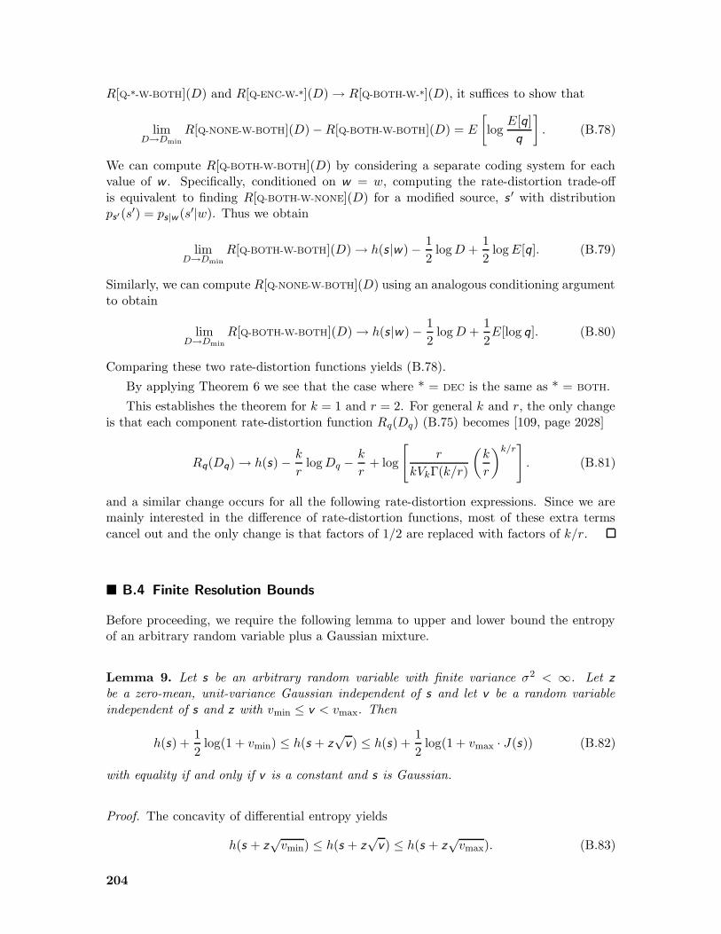
R[Q-*-W-BOTH](D) and R[Q-ENC-W-*](D)→ R[Q-BOTH-W-*](D), it suffices to show that

limD→Dmin

R[Q-NONE-W-BOTH](D)−R[Q-BOTH-W-BOTH](D) = E

[

logE[q]

q

]

. (B.78)

We can compute R[Q-BOTH-W-BOTH](D) by considering a separate coding system for eachvalue of w . Specifically, conditioned on w = w, computing the rate-distortion trade-off

is equivalent to finding R[Q-BOTH-W-NONE](D) for a modified source, s ′ with distributionps′(s

′) = ps|w (s′|w). Thus we obtain

limD→Dmin

R[Q-BOTH-W-BOTH](D)→ h(s|w)− 1

2log D +

1

2log E[q]. (B.79)

Similarly, we can compute R[Q-NONE-W-BOTH](D) using an analogous conditioning argument

to obtain

limD→Dmin

R[Q-BOTH-W-BOTH](D)→ h(s|w)− 1

2log D +

1

2E[log q]. (B.80)

Comparing these two rate-distortion functions yields (B.78).

By applying Theorem 6 we see that the case where * = DEC is the same as * = BOTH.

This establishes the theorem for k = 1 and r = 2. For general k and r, the only change

is that each component rate-distortion function Rq(Dq) (B.75) becomes [109, page 2028]

Rq(Dq)→ h(s)− k

rlog Dq −

k

r+ log

[

r

kVkΓ(k/r)

(k

r

)k/r]

. (B.81)

and a similar change occurs for all the following rate-distortion expressions. Since we aremainly interested in the difference of rate-distortion functions, most of these extra terms

cancel out and the only change is that factors of 1/2 are replaced with factors of k/r.

� B.4 Finite Resolution Bounds

Before proceeding, we require the following lemma to upper and lower bound the entropyof an arbitrary random variable plus a Gaussian mixture.

Lemma 9. Let s be an arbitrary random variable with finite variance σ2 < ∞. Let z

be a zero-mean, unit-variance Gaussian independent of s and let v be a random variable

independent of s and z with vmin ≤ v < vmax. Then

h(s) +1

2log(1 + vmin) ≤ h(s + z

√v) ≤ h(s) +

1

2log(1 + vmax · J(s)) (B.82)

with equality if and only if v is a constant and s is Gaussian.

Proof. The concavity of differential entropy yields

h(s + z√

vmin) ≤ h(s + z√

v) ≤ h(s + z√

vmax). (B.83)

204

For the lower bound we have

h(s + z√

vmin) =

∫ vmin

0

δ

δτh(s + z

√τ)dτ + h(s) (B.84)

=

∫ vmin

0

1

2J(s + z

√τ)dτ + h(s) (B.85)

≥ 1

2

∫ vmin

0J(z√

σ2 + τ)dτ + h(s) (B.86)

=1

2

∫ vmin

0

dτ

σ2 + τ+ h(s) (B.87)

=1

2log(

1 +vmin

σ2

)

(B.88)

where (B.85) follows from de Bruijn’s identity [46, Theorem 16.6.2], [51, Theorem 14], (B.86)

follows from the fact that a Gaussian distribution minimizes Fisher Information subject toa variance constraint, and (B.87) follows since the Fisher Information for a Gaussian is the

reciprocal of its variance.

Similarly, for the upper bound we have

h(s + z√

vmax) =

∫ vmax

0

δ

δτh(s + z

√τ)dτ + h(s) (B.89)

=

∫ vmax

0

1

2J(s + z

√τ)dτ + h(s) (B.90)

≤ 1

2

∫ vmax

0

J(s)J(z√

τ)

J(s) + J(z√

τ)dτ + h(s) (B.91)

=1

2

∫ vmax

0

J(s)dτ

τJ(s) + 1+ h(s) (B.92)

=1

2log (1 + vmax · J(s)) (B.93)

where (B.90) again follows from de Bruijn’s identity, (B.91) follows from the convolution

inequality for Fisher Information [24], [46, p.497], and (B.92) follows since the Fisher Infor-mation for a Gaussian is the reciprocal of its variance.

Combining these upper and lower bounds yields the desired result. Finally, the inequal-

ities used in (B.86) and (B.91) are both tight if and only if s is Gaussian.

As an aside we note that Lemma 9 can be used to bound the rate-distortion functionof an arbitrary unit-variance source, s, relative to quadratic distortion. Specifically using

an additive Gaussian noise test-channel s = z + s and combining Lemma 9 to upper boundh(s + z) with the Shannon Lower Bound [109] yields

h(s)− 1

2log 2πeD ≤ R(D) ≤ h(s)− 1

2log 2πeD +

1

2log[1 + DJ(s)]. (B.94)

Evidently, the error in the Shannon Lower Bound is at most 12 log[1 + DJ(s)] and the

sub-optimality of an additive Gaussian noise test-channel is at least 12 log[1 + D].

Proof of Theorem 9: Starting with the bound for the rate gap from (B.29), we have

R[Q-ENC-W-DEC](D)−R[Q-BOTH-W-BOTH](D) ≤ h(s + z|w)− h(s|w) (B.95)

205

=

∫

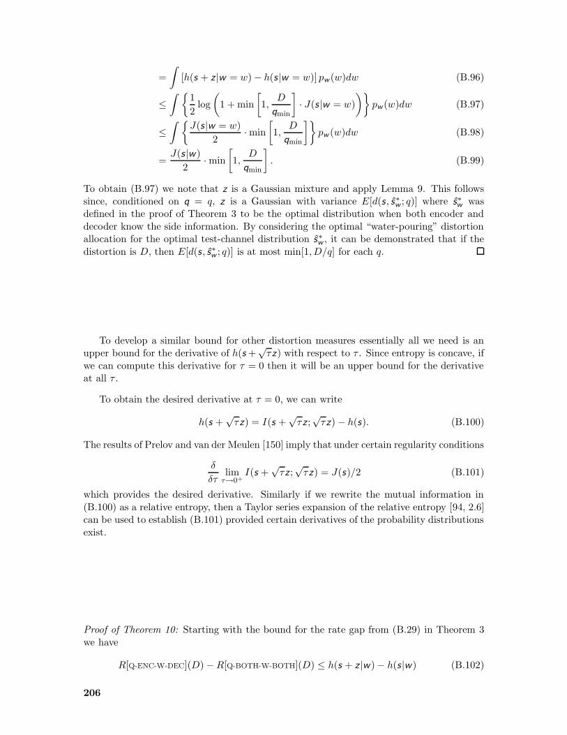
[h(s + z|w = w)− h(s|w = w)] pw(w)dw (B.96)

≤∫ {

1

2log

(

1 + min

[

1,D

qmin

]

· J(s|w = w)

)}

pw(w)dw (B.97)

≤∫ {

J(s|w = w)

2·min

[

1,D

qmin

]}

pw (w)dw (B.98)

=J(s|w)

2·min

[

1,D

qmin

]

. (B.99)

To obtain (B.97) we note that z is a Gaussian mixture and apply Lemma 9. This followssince, conditioned on q = q, z is a Gaussian with variance E[d(s, s∗w ; q)] where s∗w wasdefined in the proof of Theorem 3 to be the optimal distribution when both encoder and

decoder know the side information. By considering the optimal “water-pouring” distortionallocation for the optimal test-channel distribution s∗w , it can be demonstrated that if the

distortion is D, then E[d(s, s∗w ; q)] is at most min[1,D/q] for each q.

To develop a similar bound for other distortion measures essentially all we need is anupper bound for the derivative of h(s +

√τz) with respect to τ . Since entropy is concave, if

we can compute this derivative for τ = 0 then it will be an upper bound for the derivativeat all τ .

To obtain the desired derivative at τ = 0, we can write

h(s +√

τz) = I(s +√

τz;√

τz)− h(s). (B.100)

The results of Prelov and van der Meulen [150] imply that under certain regularity conditions

δ

δτlim

τ→0+I(s +

√τz;√

τz) = J(s)/2 (B.101)

which provides the desired derivative. Similarly if we rewrite the mutual information in

(B.100) as a relative entropy, then a Taylor series expansion of the relative entropy [94, 2.6]can be used to establish (B.101) provided certain derivatives of the probability distributions

exist.

Proof of Theorem 10: Starting with the bound for the rate gap from (B.29) in Theorem 3

we have

R[Q-ENC-W-DEC](D)−R[Q-BOTH-W-BOTH](D) ≤ h(s + z|w)− h(s|w) (B.102)

206

= D(s|w ||N (σ2s|w ))−D(s + z|w ||N (σ2

s|w + σ2z |w))

+ h(N (σ2s|w + σ2

z |w )|w)− h(N (σ2s|w )|w) (B.103)

≤ D(s|w ||N (σ2s|w )) + h(N (σ2

s|w + σ2z |w)|w)− h(N (σ2

s|w )|w) (B.104)

= D(s|w ||N (σ2s|w ))

+

∫ [

h(N (σ2s|w + σ2

z |w)|w = w)− h(N (σ2s|w )|w = w)

]

pw(w)dw (B.105)

≤ D(s|w ||N (σ2s|w )) +

∫[

1

2log

(

1 +σ2

z |w

σ2s|w

)]

pw(w)dw (B.106)

≤ D(s|w ||N (σ2s|w )) +

∫[

1

2log

(

1 +σ2

max

σ2s|w

)]

pw(w)dw (B.107)

≤ D(s|w ||N (σ2s|w )) +

∫ [1

2log

(

1 +σ2

max

σ2min

)]

pw (w)dw (B.108)

= D(s|w ||N (σ2s|w )) +

1

2log

(

1 +σ2

max

σ2min

)

. (B.109)

To obtain (B.103)–(B.106) we use the same arguments as in (B.31)–(B.37) plus the addi-tional observation that relative entropy is positive and can be dropped in obtaining (B.104).

Next, we note that there is never any need to choose the variance of the test-channel noiseto be larger than σ2

max to get (B.107). Finally, the assumption that σ2s|w ≥ σ2

min yields

(B.108).

To develop a similar bound for other distortion measures, we would use an entropy

maximizing distribution for the appropriate distortion measure in D(s|w ||·) and D(s +z||w ||·) above.

207

208

Appendix C

Iterative Quantization Proofs

209

Proof of Theorem 14: Consider quantizing a random source and choose some c > 0 and letd be the smallest integer such that at least c·n parity checks have degree at most d. For each

such parity check, the probability that all variables in the check are not erased is at least(1− e)d. Hence the probability that the check cannot be satisfied is at least (1/2) · (1− e)d.Since there are c · n such checks, the probability that at least one check cannot be satisfied

is

Pr[encoding failure] ≥ 1−[

1− (1/2) · (1− e)d]c·n

(C.1)

≥ 1−[

1− (1/2− e/2)d]c·n

(C.2)

= 1− exp{

c · n ln[

1− (1/2− e/2)d]}

(C.3)

≥ 1− exp{

−c · n · (1/2− e/2)d}

(C.4)

= 1− exp {− exp [ln c + ln n + d ln (1/2− e/2)]} . (C.5)

Hence for the probability of decoding failure to become small, d must grow at least loga-

rithmically with n for every c > 0. Note that this argument applies to any parity-checkgraph representation of the code.

Proof of Theorem 15: We will show that unique channel decoding is possible if and only ifthe matrix equation Mx = y has a solution (where M will be defined shortly). Similarly, we

will show that source quantization is possible for every z if and only if the matrix equationwM = z has a solution for every z. By demonstrating that both conditions are satisfied if

and only if the same matrix M has rank n, we will prove the desired result.

Assume that all erasures occur in the last |e| positions (i.e., e = 0n−|e| 1|e|). 1 This

incurs no loss of generality since the coordinates of C can always be permuted accordinglyand the theorem applied to the permuted code and its permuted dual code. Let x representthe transmitted signal and let y denote the received signal. Optimal decoding corresponds

to finding a vector which is a codeword of C and consistent with the unerased receivedvalues. The requirement that x is a codeword corresponds to the equation Hx = 0 where

H is the parity check matrix of C. The requirement that x is consistent with the received

unerased data corresponds to the equation (In−|e| 0)x = yn−|e|1 where It represents a t-

by-t identity matrix and y ji represents the sub-vector (yi, yi+1, . . . , yj). Thus successful

decoding is possible if and only if the equation

(In−|e| 0

H

)

x =

(

yn−|e|1

0

)

(C.6)

has a unique solution. According to well-known properties of linear algebra, uniqueness isequivalent to the matrix in (C.6) having full column rank (i.e., rank n). Note that existence

of a solution is guaranteed since a codeword was sent and no errors occurred.

Let z represent the source to be quantized with erasure pattern e⊥. Since we assumedthat all erasures in e occurred in the last |e| samples, the dual erasure pattern e⊥ has

all erasures occurring in the first |e⊥| positions (i.e., e⊥ = 1n−|e| 0|e|). Optimal decodingcorresponds to finding a vector w which is a codeword of C and consistent with the unerased

1We use |a| to denote the number of non-zero values in a (i.e., the weight of a) and bc ∆= (b b . . . b)

| {z }

c times

.

210

received values. The former requirement corresponds to the equation vG⊥ = w where G⊥

is the generator matrix of C⊥ and v is a binary vector of appropriate dimension. The latter

requirement corresponds to the equation u(

I|e⊥| 0)

+ w = z where u is a binary vector

chosen to ensure that the first |e⊥| positions (i.e., the erased positions) match regardless ofw. Thus successful decoding is possible for every z if and only if a solution exists for

(u v

)(

I|e⊥ | 0

G⊥

)

= z (C.7)

for every z. According to well-known properties of linear algebra, existence of a solution forevery z is equivalent to the matrix in (C.7) having full column rank (i.e., rank n). Note that

uniqueness of a solution is neither guaranteed not required since quantization is successfulif at least one solution is found.

Noting that G⊥ = H and |e⊥| = n − |e| completes the proof since these conditionsimply that the matrices in (C.6) and (C.7) are identical.

Proof of Theorem 16: For the algorithm to exit the while loop and reach step 8, everyunerased element of zi must have been erased in step 3 and assigned a reserved message

variable. After a variable is reserved all its checks must be erased. Since checks can neverchanged from erased to unerased, a reserved variable can never again be selected in step 2and thus a variable can never be reserved more than once.

Thus after the while loop, each unerased position in z has a corresponding reserved

variable. Hence there exists an assignment of the message variables which result in acodeword matching z in the unerased positions. This assignment could be computed via

brute-force by solving he corresponding system of linear equations, but in Theorem 18 weshow that this step can be computed more efficiently.

Proof of Theorem 17: The proof relies on the following invariant for steps 1–7 of both al-gorithms:

∀j, yj is erased if and only if zj is unerased. (C.8)

This condition is trivially true before the algorithm begins and forms the base case for a

proof by induction. We assume that (C.8) holds at iteration i of steps 1–7 and show thatit must also hold at iteration i + 1.

First, (C.8) implies that the outcome of step 1 is the same for each algorithm. Next,since G⊥ = H the tests in step 1 and step 2 of ERASURE-DECODE(H,y) and ERASURE-

QUANTIZE(G⊥, z) yield the same result. Finally, at step 3, yj is unerased while zj iserased. Therefore, by induction, condition (C.8) is true at every iteration and ERASURE-

DECODE(H,y) fails at step 5 if and only if ERASURE-QUANTIZE(G⊥, z) fails at step 5.

Proof of Theorem 18: The while loop executes at most n times. Therefore step 1 requires at

most O (n) operations. Consider storing the number of variables with exactly one unerasedcheck in a data structure which supports insertion and removal in constant time (e.g., ahash table). We can initialize the data structure with O (d · n) operations. Removing an

element in steps 2 and 3 and updating the data structure to account for step 3 requiresO (d) operations. Thus steps 1 through 8 require O (d · n) operations and all that remains

is to bound the running time of step 9.

Denote the first reserved variable by vj(1), the second reserved variable by vj(2) and soon to vj(|e|). As described in step 9, we first assign a value to vj(|e|) and work backward.

211

Specifically, we set vj(i) to the modulo-2 sum of zj(i) and all message variables connectedto zj(i) (except vj(i)). This is possible for zj(|e|) since no other reserved variable could be

connected to zj(|e|).2 Similarly, zj(|e|−1) must be connected to only unreserved variables as

well as perhaps to vj(|e|) and therefore a value can be determined for vj(|e|−1). Thus, byinduction we can determine every vj .

Adding up the operations computed for each step yields a running time of O (d · n).

2If zj(|e|) was connected to another reserved variable v, that would imply v was reserved when connectedto zj(|e|) which was unerased as well as z which must also have been unerased. This contradicts step 2 inERASURE-QUANTIZE.

212

Appendix D

Information/Operational R(D)Equivalence

213

Proposition 3. The information/operational feedforward rate-distortion functions are equal.

Proof. Since the decoder must deterministically produce s [i] from s [ i−11 ] and the nR bits

produced by the encoder we have

nR ≥n∑

i=1

H (s [i] |s [ i−11 ]) (D.1)

≥n∑

i=1

[H (s [i] |s [ i−11 ])−H (s [i] |s [ i

1 ])] (D.2)

=

n∑

i=1

[H(s [i] |s [ i−11 ])−H(s [i] |s [ i−1

1 ] , s [i])] (D.3)

=

n∑

i=1

[H(s [i])−H(s [i] |s [ i−11 ] , s [i])] (D.4)

≥n∑

i=1

[H(s [i])−H(s [i] |s [i])] (D.5)

where (D.4) follows since the source is memoryless and (D.5) follows since conditioningreduces entropy. From this point standard convexity arguments establish that (5.1) is a

lower bound to the average rate.

214

Appendix E

Proofs For Burst-Delay Codes

215

Proof of Lemma 2: Based on (7.20) there are at most

2nc·R/M ·(

2nc·[R/M−M·I(x ;y |θ=θB)]/(L−1))B

(E.1)

possible values for the unknown source components. The correct combination will always be

jointly typical with the bin index. The probability that a particular incorrect combinationof source components is typical is exactly the inverse of the number of possible bin indexes:

2−nc·[I(x ;y |θ=θG)−ε]. (E.2)

Thus the probability that any incorrect combination is jointly typical is at most

2nc·R/M ·(

2nc·[R/M−I(x ;y |θ=θB)]/(L−1))B

· 2−nc·[I(x ;y |θ=θG)−ε]. (E.3)

Provided R < CB,T − M · ε, the exponent is strictly less than

nc ·[CB,T − εM

M+ (CB,T − Mε) · B

(L− 1)M− B

L− 1· I(x ; y |θ = θB)− I(x ; y |θ = θG) + ε

]

(E.4)

= nc

{

− Bε

L− 1+ I(x ; y |θ = θG)−

B

M(B + T)· [I(x ; y |θ = θG)− I(x ; y |θ = θB)]

+B

L− 1· [I(x ; y |θ = θG)− I(x ; y |θ = θB)]

− B2

(B + T)M(L − 1)· [I(x ; y |θ = θG)− I(x ; y |θ = θB)]− I(x ; y |θ = θG)

}

(E.5)

= nc

{

− Bε

L− 1

+ [I(x ; y |θ = θG)− I(x ; y |θ = θB)] ·[

B

L− 1− B

M(T + B)− B2

M(T + B)(L− 1)

]

(E.6)

= nc

{

− Bε

L− 1

+ B · I(x ; y |θ = θG)− I(x ; y |θ = θB)

M(T + B)(L− 1)· [M(T + B)− (L− 1)− B]

}

(E.7)

= −ncBε

L− 1. (E.8)

Thus for R < CB,T − M · ε, the probability of error is at most

2−ncBε

L−1 (E.9)

which goes to zero asymptotically with nc.

216

Appendix F

Proofs for Burst Correcting CodeConstructions

217

Proof of Theorem 24: Imagine that a convolutional packet code is constructed from a blockcode C using the structure in Fig. 8-2 and consider a burst of length B starting at time

i. Since the resulting convolutional packet code is time invariant, showing that s [i] canbe recovered by time i + T is sufficient to establish the desired result. We do this byseparately considering the k source components sj[i] with j ∈ {0, 1, . . . , k − 1}. Each such

source component is the jth component in a different “diagonal block code” as illustratedin Fig. F-1.

In general, sj[i] is the jth symbol in w [i + k − 1− j]. The burst starting at x [i] affectswj [i+ k− 1− j] through wj+B−1[i+ k− 1− j] and can be recovered once wj+B[i+ k− 1− j]

through wj+T[i + k − 1− j] are received by the assumption about the delay C requires tocorrect a burst of length B. Since wj+T[i + k− 1− j] is an element of x [i + T], we have thatsj [i] is recovered with delay T.

x [i− 2] =(

s0[i− 2] s1[i− 2] s2[i− 2] s0[i− 5]⊕ s2[i− 3] s1[i− 5]⊕ s2[i− 4])

x [i− 1] =(

s0[i− 1] s1[i− 1] s2[i− 1] s0[i− 4]⊕ s2[i− 2] s1[i− 4]⊕ s2[i− 3])

x [i] =(

s0[i] s1[i] s2[i] s0[i− 3]⊕ s2[i− 1] s1[i− 3]⊕ s2[i− 2])

x [i + 1] =(

s0[i + 1] s1[i + 1] s2[i + 1] s0[i− 2]⊕ s2[i] s1[i− 2]⊕ s2[i− 1])

x [i + 2] =(

s0[i + 2] s1[i + 2] s2[i + 2] s0[i− 1]⊕ s2[i + 1] s1[i− 1]⊕ s2[i])

x [i + 3] =(

s0[i + 3] s1[i + 3] s2[i + 3] s0[i]⊕ s2[i + 2] s1[i]⊕ s2[i + 1])

x [i + 4] =(

s0[i + 4] s1[i + 4] s2[i + 4] s0[i + 1]⊕ s2[i + 3] s1[i + 1]⊕ s2[i + 2])

(a) A burst starting at time i affects the first two symbols of the constituent diagonal block code startingwith s0[i].

x [i− 2] =(

s0[i− 2] s1[i− 2] s2[i− 2] s0[i− 5]⊕ s2[i− 3] s1[i− 5]⊕ s2[i− 4])

x [i− 1] =(

s0[i− 1] s1[i− 1] s2[i− 1] s0[i− 4]⊕ s2[i− 2] s1[i− 4]⊕ s2[i− 3])

x [i] =(

s0[i] s1[i] s2[i] s0[i− 3]⊕ s2[i− 1] s1[i− 3]⊕ s2[i− 2])

x [i + 1] =(

s0[i + 1] s1[i + 1] s2[i + 1] s0[i− 2]⊕ s2[i] s1[i− 2]⊕ s2[i− 1])

x [i + 2] =(

s0[i + 2] s1[i + 2] s2[i + 2] s0[i− 1]⊕ s2[i + 1] s1[i− 1]⊕ s2[i])

x [i + 3] =(

s0[i + 3] s1[i + 3] s2[i + 3] s0[i]⊕ s2[i + 2] s1[i]⊕ s2[i + 1])

x [i + 4] =(

s0[i + 4] s1[i + 4] s2[i + 4] s0[i + 1]⊕ s2[i + 3] s1[i + 1]⊕ s2[i + 2])

(b) A burst starting at time i affects the second and third symbols of the constituent diagonal blockcode starting with s0[i − 1].

Figure F-1. Illustration of how a burst on a rate 3/5 convolutinal code affects the constituent interleavedblock codes.

For example, as illustrated in Fig. F-1(a), s0[i] corresponds to v2[i + k − 1] in Fig. 8-2

and is encoded with the block

v [i + k − 1] = (s0[i], s1[i + 1], s2[i + 2], . . . , sk−1[i + k − 1]) (F.1)

218

to yield w [i + k − 1]. The burst erases x [i], x [i + 1], . . ., x [i + B− 1], or equivalently thefirst B symbols of the constituent block code (i.e., v2[i+k−1], v2[i+k−1], . . ., v2[i+k−1]).

Thus by the assumption about the delay C requires, v2[i + k − 1] can be recovered oncev2[i + k − 1], v2[i + k − 1], . . ., v2[i + k − 1] are received. Thus, s0[i] can be recovered oncethe unerased packets up to and including s [i + T] are received and s0[i] is recovered with

the appropriate delay.A similar argument follows for s1[i] as shown in Fig. F-1(b). Specifically, s1[i] corresponds

to v2[i + k − 2] in Fig. 8-2 and is encoded with the block

v [i + k − 2] = (s1[i], s2[i + 1], s3[i + 2], . . . , sk−1[i + k − 2]) (F.2)

to yield w [i + k − 2]. The burst erases v2[i + k− 2], v2[i + k− 2], . . ., v2[i+ k− 2]. Thus by

the assumption about the delay C requires, v2[i+ k− 2] can be recovered once v2[i+ k− 2],v2[i + k − 2], . . ., v2[i + k − 2] are received. Thus, s1[i] can be recovered once the unerasedpackets up to and including s [i + T] are received and s1[i] is recovered with the appropriate

delay.

Thus we see that in general sj [i] is part of a constituent block code with the burstaffecting symbols j through j +B−1 of the block code. By our assumption about the burstcorrecting capabilities of the block code, such bursts can be corrected with the appropriate

delay. So the burst correcting abilities of the block code translate into similar abilities forthe convolutional code.

Proof of Theorem 26: First imagine that a burst of length B = n− k occurs on the secondstream in the code construction in Fig. 8-5 (i.e., the burst affects x2,j). Since the entire first

stream is received correctly, its effect on the second stream can be computed and subtractedout. Thus any burst of length n−k on the second stream can be decoded with the requireddelay by the argument used for a single link code in Theorem 25.

Next, consider a burst of length B = n− k occurring at time i on the first stream (i.e.,

x1,i, x1,i+1, . . ., x1,i+B−1). Since the source symbols for the second stream are systematicallyencoded, the corresponding parity symbols can be computed and subtracted out from x2,j .Thus the decoder effectively receives the unerased symbols from the first stream as well as

the linear combination of the parity check symbols output from the top single-link code inFig. 8-5 with s1,k−n/2, s1,k−n/2+1, . . ., s1,n/2−1. The unerased symbols in s1,k−n/2, s1,k−n/2+1,

. . ., s1,n/2−1 can be subtracted out of this linear combination.After these two subtractions, the decoder effectively receives the output of a single-link

code with input s1,0, s1,1, . . ., s1,k−n/2−1 except for B “virtually erased” symbols startingat time i. We use the term virtually erased since these symbols are not truly erased, butreceived linearly combined with erased symbols and thus not useful. In any case, the loss of

the virtually erased symbols can be corrected with the required delay using the argumentsfrom Theorem 25.

Finally, once s1,0, s1,1, . . ., s1,k−n/2−1 are decoded, the corresponding parity check sym-bols for the output of the top single-link encoder in Fig. 8-5 can be computed and subtracted

from the second stream. At this point the second stream contains s1,k−n/2, s1,k−n/2+1, . . .,s1,n/2−1 and thus these symbols are recovered with the appropriate delay.

Proof of Theorem 27: Imagine that a burst occurs on the last stream. Then the data for all

the other streams is correctly received and can be subtracted off. Thus since the single-linkcode for the last stream is optimal, the burst can be corrected with the required delay. If

219

a burst occurs on any stream j < M, then the data for all streams except j and the laststream are received and can be subtracted off. The argument to show that the remaining

two streams can be correctly recovered is then the same as for Theorem 26.

220

Appendix G

Proofs For Delay Universal StreamingCodes

221

Proof of Lemma 6: We have the following chain of inequalities:

N · nc · R < Id[if , R|θ] (G.1)

=

if∑

i=is

[ncR− I(x [i] ; y [i] |θ [i])] (G.2)

= (if − is + 1)ncR− I(

x[

ifis

]

; y[

ifis

] ∣∣θ

[ifis

])

(G.3)

= (if − is + 1)ncR− I(

x[

ifis

]

; y[

if−∞

] ∣∣θ

[if−∞

])

(G.4)

≤ (if − is + 1)ncR− I(

s[

ifis

]

; y[

if−∞

] ∣∣θ

[if−∞

])

(G.5)

≤ (if − is + 1)ncR− I(

s[

if−N

is

]

; y[

if−∞

] ∣∣θ

[if−∞

])

(G.6)

I(

s[

if−N

is

]

; y[

if−∞

] ∣∣θ

[if−∞

])

< (if − is −N + 1)ncR. (G.7)

Equations (G.1) and (G.2) follow from the assumption that Id[i, R|θ] > ncRN for is ≤ i ≤ if .

The chain rule for mutual information and the block memoryless structure of the channelyield (G.3) and (G.4). Equation (G.5) follows from the data processing inequality and (G.6)follows from the chain rule for mutual information.

Finally, we can consider s [is], s [is + 1], . . ., s [if −N ] as a message of rate (if − is −N + 1) · R. Therefore Fano’s inequality combined with (G.7) implies that the decoder cannot recover this message with small probability of error.

Proof of Lemma 7: Consider the greedy channel state sequence θ∗ where first θ∗ [is] is cho-

sen to maximize the information debt when it becomes positive at time is, next θ∗ [is + 1] ischosen to maximize Id[is +1, R|θ∗], and then θ∗ [is + 2] is chosen to maximize Id[is +2, R|θ∗],etc, until Id[i, R|θ∗] becomes non-positive at time is + T and stays non-positive for at least

the next T times.1 By construction, this choice for θ∗ [i] maximizes the right hand side of(9.10).

Without loss of generality, let is = 0, and assume, for the sake of contradiction, that

some code, C, achieves a lower delay than (9.10). Then, with this code, s [0], can be decodedat or before time T−1 when Id[T−1, R|θ∗] = δ > 0. Define the new channel state sequences

θ∗∗ and θ

∗∗′ by letting θ∗∗ = θ

∗, θ∗∗′ = θ

∗ except that θ∗∗′[T] = θ∗ [0], θ∗∗ [T] = θ∗ [0],

and θ∗∗ [0] = θ∗ [T]. The relationships between these channel state sequences and others wedefine shortly are illustrated in Table G.1.

Table G.1. The relationship between various channel state sequences used in the proof. Sequences withoutthe prime symbol (′) are elements of Θ, while those with primes may not be in Θ, but must be decodablewith delay no more than the corresponding unprimed sequence.

θ∗ = θ∗ [−1] θ∗ [0] θ∗ [1] θ∗ [2] . . . θ∗ [T− 1] θ∗ [T] θ∗ [T + 1] θ∗ [T + 2] θ∗ [T + 3]

θ∗∗ = θ∗ [−1] θ∗ [T] θ∗ [1] θ∗ [2] . . . θ∗ [T− 1] θ∗ [0] θ∗ [T + 1] θ∗ [T + 2] θ∗ [T + 3]

θ∗∗′ = θ∗ [−1] θ∗ [0] θ∗ [1] θ∗ [2] . . . θ∗ [T− 1] θ∗ [0] θ∗ [T + 1] θ∗ [T + 2] θ∗ [T + 3]

θ∗∗∗ = θ∗ [−1] θ∗ [T] θ∗ [T + 1] θ∗ [2] . . . θ∗ [T− 1] θ∗ [0] θ∗ [1] θ∗ [T + 2] θ∗ [T + 3]

θ∗∗∗′ = θ∗ [−1] θ∗ [0] θ∗ [1] θ∗ [2] . . . θ∗ [T− 1] θ∗ [0] θ∗ [1] θ∗ [T + 2] θ∗ [T + 3]

1If it is not possible to choose θ in a permutation invariant set such that Id[i, R|θ] stays non-positive forat least T times, then it is possible to show that Id[i, R|θ ] eventually becomes bounded away from 0 and thedecoding delay grows to infinity.

222

Note that while θ∗∗ ∈ Θ by the permutation invariance of Θ, technically θ

∗∗′ may notbe in Θ. However, since s [0] can be decoded before time T, to the decoder it is as if s [0] is

known perfectly by time T and hence the decoding delay for the state sequence θ∗∗′ must

be no greater than for θ∗∗. Specifically, the decoder must be able to recover s [1] by time

T + 1. Furthermore, since θ∗ [0] was chosen to maximally increase the information debt

while θ∗ [T + 1] was chosen to not increase it,

I (x [T + 1] ; y [T + 1] |θ∗ [T + 1])− I (x [0] ; y [0] |θ∗ [0]) > δ

and hence Id[T + 1, R|θ∗∗′ ] must be at least 2δ.

Next, define the new channel state sequences θ∗∗∗, θ

∗∗∗′ by letting θ∗∗∗ = θ

∗∗, andθ∗∗∗′ = θ

∗∗′ , except that θ∗∗∗ [T + 1] = θ∗ [1], θ∗∗∗′[T + 1] = θ∗ [1], and θ∗∗∗ [1] = θ∗ [T + 1].

Once again, θ∗∗∗′ may not be in Θ, but θ

∗∗∗ is in Θ, and the decoding delay for these two isequivalent since we have already shown s [0] is recovered by time T−1 and s [1] is receoveredby time T. Also, using similar reasoning as before, since θ∗ [1] was chosen to maximally

increase the information debt while θ∗ [T + 2] was chosen to not increase it,

I (x [T + 2] ; y [T + 2] |θ∗ [T + 2])− I (x [1] ; y [1] |θ∗ [1]) > 0

and hence Id[T + 2, R|θ∗∗∗′ ] must still be at least 2δ.

We can continue this pattern to construct the sequences,

θ∗q′

[i] =

{

θ∗ [i mod T] , 0 ≤ i ≤ T + q − 2

θ∗ [i] , otherwise(G.8)

and

θ∗q[i] =

θ∗ [i− T] , T ≤ i ≤ T + q − 2

θ∗ [i + T] , 0 ≤ i ≤ q − 2

θ∗ [i] , otherwise.

(G.9)

The latter sequence is an element of Θ and requires decoding delay at most T − 1 by

assumption. Furthermore, we can show by induction that

Id[T + q − 2, R|θ∗q ′ ] >

⌈q − 1

2T

⌉

δ.

Choose q such that d(q − 1)/(2T)e > RT/δ, and consider when s [q − 1] can be decoded

for the channel state sequence θ∗q ′ . By induction on our previous arguments, we can show

that the decoding delay for θq∗′ is no greater than for θ

q∗. Hence, the decoding delay isT − 1 and s [q − 1] can be recovered by time T + q − 2. But the information debt at time

T+ q−2 is at least RT, and according to Lemma 6, s [q − 1] can not be decoded at or beforetime T + q − 2. Therefore, it is impossible for any code to correct all patterns in Θ with

delay less than T, and the proof is complete.

Proof of Theorem 31: By assumption the random walk defined in (9.29) will satisfy therequirements for Wald’s Identity, (9.30). Taking the derivative with respect to r of both

sides of (9.30) and evaluating the result as r→ 0 yields

E[w [t]] = E[v ]E[t]. (G.10)

223

By construction, the random walk ends at time t when w [t] drops below −Id[is, R|θ] so

E[v ]E[t] = E[w [t]] ≤ −Id[is, R|θ] (G.11)

E[t] ≥ −Id[is, R|θ]

E[v ](G.12)

where the inequality changes direction due to division by E[v ] which is negative since

R < E[I (x ; y)]. Substituting the definitions of v (9.28) and Id[i, R|θ] (9.9), and taking theexpectation of Id[is, R|θ] conditioned on the fact that Id[i, R|θ] becomes positive at timei = is then yields the first term in (9.31).

Next we note that w [t − 1] > −Id[is, R|θ] by definition and therefore

w [t] = w [t − 1] + v [t] > −Id[is, R|θ] + min v .

Substituting this bound into Wald’s Identity and preceding as before yields the second termin (9.31).

Proof of Theorem 32: We begin by taking the second derivative with respect to r of Wald’s

Identity, (9.30), and evaluating the result as r→ 0:

E{w [t]2 − 2t · w [t] · E[v ] + t2 · E[v ]2 − t · VAR[v ]} = 0.

Performing some simple algebra yields

E[t2] · E[v ]2 ± E[t]2 ·E[v ]2 = −E[w [t]2]± E[w [t]]2

+2E[t · w [t]] ·E[v ] + E[t] · VAR[v ]

VAR[t] ·E[v ]2 + (E[v ] · E[t])2 = −VAR[w [t]]− E[w [t]]2

+2E[t · w [t]] ·E[v ] + E[t] · VAR[v ]

VAR[t] · E[v ]2 + 2(E[v ] · E[t])2 = −VAR[w [t]] + 2E[t · w [t]] · E[v ] + VAR[v ] · E[t]

where the last line follows from (G.10).

Next we obtain the following sequence of inequalities

VAR[t]

E[t]≤ −2E[t] − VAR[w [t]]

E[v ]2 · E[t]+

2 · E[t · (Id[is, R|θ] + min v)]

E[v ] ·E[t]+

VAR[v ]

E[v ]2(G.13)

VAR[t]

E[t]≤ −2 · Id[is, R|θ]

E[v ]− VAR[w [t]]

E[v ]2 · E[t]+

2 · Id[is, R|θ] + min v

E[v ]+

VAR[v ]

E[v ]2(G.14)

≤ VAR[v ]

E[v ]2+

min v

E[v ]. (G.15)

We obtain (G.13) by noting that w [t]/E[v ] ≤ (Id[is, R|θ] + min v)/E[v ]. Using (G.12)

yields (G.14) and (G.15) follows from the obvious fact that −VAR[w [t]] ≤ 0. Substitutingthe appropriate quantities completes the proof.

224

Proof of Theorem 33: Starting from (9.30) we have the following chain of inequalities:

1 = E[exp(r · w [t]− t · γ(r))] (G.16)

≥ E[exp(r · w [t]− t · γ(r))|t > T] · Pr[t > T] (G.17)

≥ exp(r · w [t]− T · γ(r)) · Pr[t > T], r < r∗ (G.18)

Pr[t > T] ≤ exp(−r · w [t] + T · γ(r)), r < r∗ (G.19)

where (G.18) follows since γ(r) < 0 for r < r∗ by the definition of r∗ and the assumptionthat R < E[I (x ; y)]. We obtain (9.33) by noting that

w [t] ≥ w [t − 1] + min v ≥ −Id[is, R|θ] + min v. (G.20)

To obtain (9.34), we again start from (9.30) and use the following chain of inequalities:

1 = E[exp(r · w [t]− t · γ(r))] (G.21)

≥ E[exp(r · w [t]− t · γ(r))|t < T] · Pr[t < T] (G.22)

≥ exp(r · w [t]− T · γ(r)) · Pr[t < T], r > r∗ (G.23)

Pr[t < T] ≤ exp(−r · w [t] + T · γ(r)), r < r∗ (G.24)

where (G.23) follows since γ(r) > 0 for r > r∗ by the definition of r∗ and the assumptionthat R < E[I (x ; y)]. We obtain (9.34) by again using (G.20).

225

226

Appendix H

Distortion Exponent Derivations

227

� H.1 Distortion Exponent For Selection Channel Coding Diversity

Proof of Theorem 35: The minimum expected distortion for such a scheme is computed as

follows:

E[D] = minD

Pr {max [I (x1; y1), I (x2; y2)] < R(D)}

+ Pr {max [I (x1; y1), I (x2; y2)] ≥ R(D)} ·D (H.1)

= minD

FeI (exp R(D))2 + [1− FeI (exp R(D))2] ·D (H.2)

≈ minD

c2D−pβ SNR−2p +

(

1− c2D−pβ SNR−2p

)

·D (H.3)

≈ minD

c2D−pβ SNR−2p + D. (H.4)

Differentiating and setting equal to zero yields

D∗ = SNR−2pβp+β ·

(β

pc

)−pβp+β

(H.5)

and thusE[D] ≈ CSEL−CCDIVSNR

−2pβp+β (H.6)

where CSEL−CCDIV is a constant independent of SNR.

� H.2 Distortion Exponent For Multiplexed Channel Coding Diversity

Proof of Theorem 36: The minimum expected distortion for such a scheme is computed asfollows:

E[D] = minD

Pr {min [I (x1; y1), I (x2; y2)] < R(D)}

+ Pr {min [I (x1; y1), I (x2; y2)] ≥ R(D)} ·D (H.7)

= minD

2FeI (exp[R(D)/2])− FeI (exp[R(D)/2])2 + [1− FeI (exp[R(D)/2])]2 ·D (H.8)

≈ minD

2cD−p4β SNR−p − c2D

−p2β SNR−2p +

(

1− cD−p4β SNR−p

)2·D (H.9)

≈ minD

2cD−p4β SNR−p + D (H.10)

Differentiating and setting equal to zero yields the optimizing distortion

D∗ = SNR−4pβp+4β ·

(2β

pc

) −4βp+4β

(H.11)

and thus

E[D] ≈ CMPX−CCDIVSNR−4pβp+4β (H.12)

where CMPX−CCDIV is a constant independent of SNR.

228

� H.3 Distortion Exponent for Optimal Channel Coding Diversity

Before proving Theorem 37 we require the following lemma characterizing the mutual in-formation for the parallel channel in terms of probability distribution for each sub-channel.

Lemma 10. LetI (x; y) = I (x1; y1) + I (x2; y2)

be the mutual information for the total channel and assume that the density and distribution

for each sub-channel is given by. (10.43) and (10.44) If we define the cumulative distributionfunction for exp I (x; y) as FeI0+I1(t) then

FeI0+I1(t) ≈ pc2

(t

SNR2

)p(

ln t− 1

p

)

(H.13)

in the sense that the ratio of these quantities goes to 1 as SNR→∞.

Proof. Note that for any random variable, θ with density fθ(t), we have

feθ(t) = fθ(ln t)/t and fθ(t) = feθ(et) · et. (H.14)

Therefore we can obtain the desired result by computing the pdf, fI0+I1(t), via convolution,

and applying (H.14):

fI0+I1(t) =

∫ t

0fI (τ) · fI (t− τ)dτ (H.15)

=

∫ t

0eτfeI (eτ ) · et−τfeI (et−τ )dτ (H.16)

≈∫ t

0cp

epτ

SNRp · cpep(t−τ)

SNRp dτ (H.17)

= c2p2 ept

SNR2p

∫ t

0dτ (H.18)

= c2p2tept

SNR2p(H.19)

FeI0+I1 (t) =

∫ t

−∞feI0+I1(τ)dτ (H.20)

=

∫ t

−∞

fI0+I1(ln τ)

τdτ (H.21)

≈ c2p2

SNR2p

∫ t

1τp−1 · ln τdτ (H.22)

=c2p2

SNR2p ·(

tp ln t

p− tp

p2+

1

p2

)

(H.23)

≈ pc2

(t

SNR2

)p(

ln t− 1

p

)

(H.24)

where (H.17) follows from the high SNR approximation in (10.43), (H.22) follows fromsubstituting (H.19) into (H.21) and noting that since I (x; y) is positive then fI0+I1(ln t) is

non-zero only for t > 1, and the final line follows from noting that the last parenthesizedterm in (H.23) is negligible at high SNR.

229

Proof of Theorem 37: To compute the minimum average distortion we have

E[D] = minD

Pr[I (x1; y1) + I (x2; y2) < R(D)] + {1− Pr[I (x1; y1) + I (x2; y2) < R(D)]} ·D

(H.25)

= minD

FeI0+I1(exp R(D)) + [1− FeI0+I1 (R(D))] ·D (H.26)

≈ minD

pc2 D−p2β

SNR2p

(

−β lnD − 1

p+

Dp2β

p

)

+

[

1− pc2 D−p2β

SNR2p

(

−β lnD − 1

p+

Dp2β

p

)]

·D

(H.27)

≈ minD

pc2 D−p2β

SNR2p

(

−β lnD − 1

p+

Dp2β

p

)

+ D. (H.28)

By noting that the parenthesized term in (H.28) is between 1/p and (1 + e−1)/p whenD < exp−(1/pβ), we obtain

minD

c2 D−p2β

SNR2p + D / E[D] / minD

(1 + e−1)c2 D−p2β

SNR2p + D. (H.29)

Differentiating the lower bound and setting equal to zero yields the optimizing distortion

D∗ = SNR−4pβp+2β ·

(c2p

2β

) −2βp+2β

. (H.30)

Substituting (H.30) into (H.29) yields

CLB · SNR−4pβp+2β / E[D] / CUB · SNR

−4pβp+2β (H.31)

where CLB and CUB are terms independent of SNR. Hence we conclude that the distortionexponent is

∆OPT−CCDIV = (4pβ)/(p + 2β). (H.32)

230

� H.4 Distortion Exponent for Source Coding Diversity

Proof of Theorem 38: For small D0 and D1, the average distortion is

E[D] = minD0,D1

Pr[I (x1; x2) < Rmd(D0,D1)/2]2

+ 2Pr[I (x1; x2) < Rmd(D0,D1)/2] · Pr[I (x1; x2) ≥ Rmd(D0,D1)/2] ·D1

+ Pr[I (x1; x2) ≥ Rmd(D0,D1)/2]2 ·D0 (H.33)

= minD0,D1

FeI (exp Rmd(D0,D1)/2)2

+ 2 · FeI (exp Rmd(D0,D1)/2) · [1− FeI (exp Rmd(D0,D1)/2)] ·D1

+ [1− FeI (exp Rmd(D0,D1)/2)]2 ·D0 (H.34)

≈ minD0,D1

c2

SNR2p exp {p ·Rmd(D0,D1)}

+ 2c

SNRp exp{p

2·Rmd(D0,D1)

}

·[

1− c

SNRp exp{p

2·Rmd(D0,D1)

}]

·D1

+[

1− c

SNRp exp{p

2·Rmd(D0,D1)

}]2·D0 (H.35)

≈ minD0,D1

c2

SNR2p exp {p ·Rmd(D0,D1)}+ 2c

SNRp exp{p

2·Rmd(D0,D1)

}

·D1 + D0.

(H.36)

Substituting the bounds from (10.30) into (H.36) yields

E[D] / minD1,D0

c2

SNR2p

(1

2D1D0

) p2β

+2c

SNRp

(1

2D1D0

) p4β

·D1 + D0 (H.37a)

E[D] ' minD1,D0

c2

SNR2p

(1

4D1D0

) p2β

+2c

SNRp

(1

4D1D0

) p4β

·D1 + D0 (H.37b)

where (H.37b) requires D0 → 0 and (H.37a) also requires D1 → 0.

When p ≥ 4β then (H.37) increases as D1 becomes small. Hence in this regime the

optimal choice for D1 approaches a constant bounded away from zero. If the low distor-tion formula for the lower bound is used, then the optimal choice for D1 approaches one.

Technically, however, for D1 ≥ 1/2 the rate required is given by (10.26b) not (10.26a), sothere is no excess rate in multiple description coding [71,76] and the optimal D1 for p ≥ 4βapproaches 1/2 using (10.26b). In any case, regardless of whether D1 = 1/2 or D1 = 1 or

some other intermediate value, when p ≥ 4β, average distortion is minimized by choosingD1 to be large. Thus for p ≥ 4β, the optimal multiple description system essentially de-

generates into the channel multiplexing scheme analyzed in Section 10.4.4 and achieves thesame distortion exponent (although with a slightly different constant factor term).

When p < 4β, we can find the optimal value for D1 by differentiating the lower boundwith respect to D1 and setting equal to 0 to obtain

D∗1 =

(4β − p

cp

) −4β4β−p

· SNR−4βp4β+p · (4D0)

−1+ 4β4β+p , p < 4β. (H.38)

231

For the case when p < 4β, substituting (H.38) into (H.37b) yields

E[D] ' C ·D−2p4β+p

0 · SNR−8pβ4β+p + D0 for p < 4β (H.39)

where C is a constant independent of SNR and D0. Differentiating with respect to D0 andsetting the result equal to zero yields the optimal value for D0:

D∗0 =

C ′ · SNR−8βp4β+3p , p < 4β

C ′′ · SNR−4βp4β+p , p ≥ 4β

(H.40)

from which we conclude

CLB · SNR−max

h

8βp4β+3p

, 4βp4β+p

i

/ E[D] / CUB · SNR−max

h

8βp4β+3p

, 4βp4β+p

i

(H.41)

where the max occurs since multiple description coding essentially degenerates into channel

multiplexing with a better constant factor when p ≥ 4β.

� H.5 Distortion Exponent for Source Coding Diversity with Joint Decoding

Computing the exact rates required to guarantee successful encoding in (10.65) is generally

difficult, thus we focus on the high resolution limit in the following Lemma.

Lemma 11. Let s be a source with finite variance and finite entropy power. Then in the

high resolution limit, choosing

R > h(s)− (1/2) log 2πeσ2 (H.42)

asymptotically satisfies (10.65) and guarantees successful encoding.

Proof. Proving the claim requires showing that

limDj→0

I(s; sj)−[

h(s)− 1

2log 2πeσ2

]

= 0 for j ∈ {0, 1} (H.43)

and

limDj→0

I(s; s1s2) + I (s1; s2)− 2

[

h(s)− 1

2log 2πeσ2

]

= 0. (H.44)

The former follows from the fact that the Shannon Lower Bound is asymptoticallytight [109]. In the interest of completeness, however, we define ∆R as left hand side of

232

(H.43) and summarize the argument showing that it goes to zero:

∆R∆= lim

Dj→0I(s; sj)−

[

h(s)− 1

2log 2πeσ2

]

(H.45)

= limDj→0

h(s + nj)− h(s + nj |s)−[

h(s)− 1

2log 2πeσ2

]

(H.46)

= limDj→0

h(s + nj)− h(nj)−[

h(s)− 1

2log 2πeσ2

]

(H.47)

= limDj→0

h(s + nj)− h(s) (H.48)

= 0. (H.49)

Equations (H.46) and (H.47) follow from the choice of the conditional distribution sj = s+nj

where nj is independent of s. The key step in going from (H.48) to (H.49) is the “continuity”property of differential entropy [109, Theorem 1] which is the main tool in obtaining many

high-resolution source coding results.

A similar chain of equalities establishes (H.44). Specifically, if we define the right handside of (H.44) as ∆2R then we obtain

∆2R∆= lim

Dj→0I(s; s1s2) + I (s1; s2)− 2

[

h(s)− 1

2log 2πeσ2

]

(H.50)

= limDj→0

h(s1s2)− h(s1s2|s) + h(s1)− h(s1|s2)− 2

[

h(s)− 1

2log 2πeσ2

]

(H.51)

= limDj→0

h(s1) + h(s2)− h(s1|s)− h(s2|s)− 2

[

h(s)− 1

2log 2πeσ2

]

(H.52)

= limDj→0

2 ·∆R (H.53)

= 0 (H.54)

where (H.53) follows by noting that (H.52) is simply twice (H.45), and hence (H.54) followsfrom (H.49).

In the sequel, we require the following Lemma which states that, in the high resolutionlimit, the two descriptions, s1 and s2, only differ in half a bit per sample. This close relation-

ship between the two descriptions enables the joint decoder to approach the performanceof parallel channel coding with a single description.

Lemma 12. If the rate is chosen according to (H.42), specifically, if the difference between

the two sides is ε, then

limDj→0

I (s1; s2)−R ≥ −1

2log 2− ε. (H.55)

233

Proof. We have the following chain of inequalities:

limDj→0

I (s1; s2)−R = limDj→0

h(s + n1)− h(s + n1|s + n2)−R (H.56)

= limDj→0

h(s + n1)− h(n1 − n2|s + n2)−R (H.57)

≥ limDj→0

h(s + n1)− h(n1 − n2)−R (H.58)

= limDj→0

h(s + n1)−1

2log 4πeσ2 −R (H.59)

= limDj→0

h(s + n1)− h(n1)−1

2log 2−R (H.60)

= limDj→0

I (s1; s)−R− 1

2log 2 (H.61)

= limDj→0

I (s1; s)−[

h(s)− 1

2log 2πe + ε

]

− 1

2log 2 (H.62)

= limDj→0

∆R− 1

2log 2− ε (H.63)

= −1

2log 2− ε. (H.64)

Most of the arguments follow from well-known properties of mutual information and entropy.Equation (H.64) follows from Lemma 11.

Proof of Theorem 40: If we choose σ2 as in (10.70), the expected distortion is at most thedistortion when both descriptions are successfully decoded times the probability that bothdescriptions are not decoded. Hence, applying Theorem 39 yields

E[D] ≤ σ2

2· Pr[E ] + Pr[Ec] (H.65)

where E denotes the event that both descriptions can be decoded as defined in (10.66) andEc is the complement of E . Note that since Pr[E ] ≤ 1, the first term on the right hand sideof (H.65) is proportional to SNR−∆OPT−CCDIV by construction due to our choice of σ2 in

(10.70). Therefore, to prove the Theorem, we need to bound the second term, Pr[E c].

If we let E [i, j] (with i, j ∈ {1, 2}) denote the event that the first max operation in Ereturns the ith argument while the second max operation in E returns the jth argument,then we can express the second term in (H.65) as

Pr[Ec] = Pr[Ec ∩ E [1, 1]|E [1, 1]] Pr[E [1, 1]] + Pr[E c ∩ E [1, 2]|E [1, 2]] Pr[E [1, 2]]

+ Pr[Ec ∩ E [2, 1]|E [2, 1]] Pr[E [2, 1]] + Pr[E c ∩ E [2, 2]|E [2, 2]] Pr[E [2, 2]]. (H.66)

To prove the theorem, it is sufficient to show that for every ε > 0, there exists a constant

ci,j such thatPr[Ec|E [i, j]] Pr[E [i, j]] ≤ ci,j · SNRε−∆OPT−CCDIV

for large enough SNR.

Conditioned on E [1, 1], both I (x1; y1) > R/β and I (x2; y2) > R/β, so both channels aregood enough to decode each description separately. Thus Pr[E c|E [1, 1]] = 0, and therefore

234

Pr[Ec|E [1, 1]] Pr[E [1, 1]] = 0 as well. This takes care of the first term in (H.66).

Next we consider the second term of (H.66). Conditioned on E [1, 2], only I (x1; y1) > R/βwhile I (x2; y2) < R/β and only description 1 can be decoded separately. Description 2 can

be decoded jointly provided that I (x2; y2) ≥ R/β−I (s1; s2)/β. By applying Lemma 12, thiscondition becomes I (x2; y2) > (log 2)/(2β) in the high-resolution limit, therefore

Pr[Ec|E [1, 2]] Pr[E [1, 2]] ≈ Pr

[

I (x2; y2) ≤log 2

2β

]

· Pr[E [1, 2]] (H.67)

≈ c ·(

212β

SNR

)p

· Pr[E [1, 2]] (H.68)

≤ c ·(

212β

SNR

)p

· Pr[I (x2; y2) < R/β] (H.69)

≈ c ·(

212β

SNR

)p

· c ·

exp

h(s)β

σ1/βSNR

p

(H.70)

= SNR−2p · SNR2p

p+2β · c2

(

212β exp

h(s)

β

)p

(H.71)

= SNR−4pβp+2β · c2

(

212β exp

h(s)

β

)p

(H.72)

where in going from (H.69) to (H.70) we replaced R with h(s)−(1/2) log 2πeσ2 and recalledthat we assumed exp[2h(s)] = 2πe just after (10.23).

Thus, for some constant CSCDIV−JD, and every ε > 0, there exists an SNR large enough

such thatPr[Ec|E [1, 2]] Pr[E [1, 2]] ≤ SNR

ε− 4pβp+2β · CSCDIV−JD (H.73)

andPr[Ec|E [2, 1]] Pr[E [2, 1]] ≤ SNRε− 4pβ

p+2β ·CSCDIV−JD. (H.74)

A similar analysis works for the third term of (H.66).

Finally, we consider the last term in (H.66). Conditioned on E [2, 2], both I (x1; y1) < R/βand I (x2; y2) < R/β, so neither channels is good enough for separate decoding. Successful

joint decoding requires

I (x1; y1) + I (x2; y2) > [2R− I (s1; s2)] /β. (H.75)

235

and therefore

Pr[Ec ∩ E [2, 2]|E [2, 2]] = Pr [I (x1; y1) + I (x2; y2) ≤ 2R/β − I (s1; s2)/β] (H.76)

/ Pr

[

I (x1; y1) + I (x2; y2) ≤ R/β − log 2

2β

]

(H.77)

≈ pc2

2

12β exp h(s)

2β

σ1/βSNR2

p

·(

h(s)

2β− log 2πeσ2

2β+

log 2

2β− 1

p

)

(H.78)

= σ−p/β · SNR−2p · 212β · exp

h(s)

2β·(

h(s)

2β− log 2πeσ2

2β+

log 2

2β− 1

p

)

(H.79)

≈ SNR−2p2

p+2β−2p2 · C ′SCDIV−JD · SNRε (H.80)

= SNRε− 4pβ

p+2β · C ′SCDIV−JD (H.81)

where (H.77) follows since Lemma 12 implies

2R− I (s1; s2) ≤ R− 1

2log 2 + ε, (H.82)

ε is a quantity which can be made arbitrarily small, and C ′SCDIV−JD is some constantindependent of SNR.

The above results combined with ∆OPT−CCDIV = 4pβ/(p+2β) proves the desired result.

236

Bibliography

[1] M. Adams and V. Guillemin. Measure Theory and Probability. Birkauser, 1996. Cited

on page 199

[2] E. Agrell, T. Eriksson, A. Vardy, and K. Zeger. Closest point search in lattices. IEEE

Transactions on Information Theory, 48(8):2201–2214, August 2002. Cited on page55, 66

[3] R. F. Ahlswede. The Rate-Distortion Region for Multiple Descriptions without ExcessRate. IEEE Trans. Inform. Theory, 31(6):721–726, November 1985. Cited on page

158, 161

[4] M. Alasti, K. Sayrafian-Pour, A. Ephremides, and N. Farvardin. Multiple Descrip-

tion Coding in Networks with Congestion Problem. IEEE Trans. Inform. Theory,47(3):891–902, March 2001. Cited on page 158, 162, 192

[5] A. Albanese, J. Blomer, J. Edmonds, M. Luby, and M. Sudan. Priority encodingtransmission. IEEE Transactions on Information Theory, 42(6):1737–1744, Nov 1996.Cited on page 22

[6] E. Altman, C. Barakat, and V. Ramos. Queueing analysis of simple fec schemes forip telephony. In INFOCOM 2001, volume 2, pages 796–804, 2001. Cited on page 22

[7] E. Altman and A. Jean-Marie. Loss probabilities for messages with redundant packetsfeeding a finite buffer. Journal of Selected Areas in Communications, 16(5):778–787,

June 1998. Cited on page 22

[8] J. Alvarez and B. Hajek. On the use of packet classes in communication networksto enhance congestion pricing based on marks. IEEE Transactions on AutomaticControl, 47(6):1020–1026, June 2002. Cited on page 22

[9] J. G. Apostolopoulos. Reliable video compression over lossy packet networks usingmultiple state encoding and path diversity. In Proc. SPIE Visual Communications

and Image Processing (VCIP), volume 4310, San Jose, CA, January 2001. Cited onpage 158, 161

[10] J. G. Apostolopoulos, W.-T. Tan, S. J. Wee, and G. W. Wornell. Modeling PathDiversity for Multiple Description Video Communications. Proc. International Con-

ference on Acoustics, Speech, and Signal Processing, May 2002. Cited on page 158,161

237

[11] J. G. Apostolopoulos, W. tian Tan, and S. J. Wee. Performance of a multiple descrip-tion streaming media content delivery network. In Proc. International Conference on

Image Processing, volume 2, pages 189–192, September 2002. Cited on page 192

[12] J. G. Apostolopoulos and S. J. Wee. Unbalanced multiple description video com-munication using path diversity. In Proc. IEEE International Conf. on Image Proc.

(ICIP), volume 1, pages 966–969, Thessaloniki, Greece, October 2001. Cited on page158

[13] M. Arai, A. Chiba, and K. Iwasaki. Measrurement and modeling of burst packetlosses in internet end-to-end communications. In Proceedings of the 1999 Pacific RimInternational Symposium on Dependable Computing, pages 260–267, 1999. Cited on

page 102

[14] N. At and Y. Altunbasak. Multiple Description Coding for Wireless Channels with

Multiple Antennas. In Proc. IEEE Global Comm. Conf. (GLOBECOM), volume 3,pages 2040–2044, San Antonio, TX, November 2001. Cited on page 158

[15] H. Balakrishnan, S. Seshan, and R. H. Katz. Improving reliable transport and handoff

performance in cellular wireless networks. ACM Wireless Networks, December 1995.Cited on page 22

[16] R. J. Barron, B. Chen, and G. W. Wornell. The duality between information embed-ding and source coding with side information and some applications. IEEE Transac-tions on Information Theory, 49(5):1159–1180, May 2003. Cited on page 84

[17] J. Barros, J. Hagenauer, and N. Gortz. Turbo Cross Decoding of Multiple Descrip-tions. In Proc. International Conference on Communications, volume 3, pages 1398–

1402, New York, NY, 20 April - 2 May 2002. Cited on page 158

[18] T. Berger. Private Communication. Cited on page 34, 35

[19] T. Berger. Rate Distortion Theory: A Mathematical Basis For Data Compression.

Prentice-Hall, Englewood Cliffs, NJ, 1971. Cited on page 31, 35, 43

[20] T. Berger and Z. Zhang. Minimum Breakdown Degradation in Binary Source Encod-

ing. IEEE Trans. Inform. Theory, 29(6):807–814, November 1983. Cited on page161

[21] T. Berger, Z. Zhang, and H. Viswanathan. The ceo problem [multiterminal source

coding]. IEEE Transactions on Information Theory, 42(3):887–902, May 1996. Citedon page 50

[22] R. A. Berry. Power and Delay Trade-Offs in Fading Channels. PhD thesis, Mas-sachusetts Institute of Technology, Cambridge, MA, June 2000. Cited on page 22

[23] E. Biglieri, J. Proakis, and S. Shamai. Fading channels: information-theoretic and

communications aspects. IEEE Transactions on Information Theory, 44(6):2619–2692, October 1998. Cited on page 22, 96, 97, 105, 140, 151

[24] N. Blachman. The convolution inequality for entropy powers. IEEE Transactions onInformation Theory, 11(2):267–271, April 1965. Cited on page 205

238

[25] D. Blackwell, L. Breiman, and A. J. Thomasian. The capacity of a class of channels.Ann. Math. Stat., 30:1229–1241, December 1959. Cited on page 24, 97, 138

[26] S. Blake, D. Black, M. Carlson, E. Davies, Z. Wang, and W. Weiss. An ar-chitecture for differentiated services. IETF RFC2475, 1998. Available online at

http://www.ietf.org/rfc/rfc2475.txt. Cited on page 22

[27] J. Bolot. Characterizing end-to-end packet delay and loss in the internet. Journal ofHigh Speed Networks, pages 289–298, September 1993. Cited on page 102

[28] J. Bolot, S. Fosse-Parisis, and D. Towsley. Adaptive fec-based error control for internettelephony. In Proc. of Infocom’99, March 1999. Cited on page 22

[29] M. S. Borella, D. Swider, S. Uludag, and G. B. Brewster. Internet packet loss: mea-surement and implications for end-to-end qos. In Proceedings of the 1998 ICPP Work-

shops on Architectural and OS Support for Multimedia Applications/Flexible Commu-nications Systems/Wireless Networks and Mobile Computing, pages 3–12, 1998. Citedon page 102

[30] V. S. Borkar, S. K. Mitter, and S. Tatikonda. Optimal sequential vector quantizationof Markov sources. SIAM J. Control Optim., 40(1):135–148, 2001. Cited on page 84,

190

[31] J. Byers, M. Luby, and M. Mitzenmacher. A digital fountain approach to asyn-

chronous reliable multicast. IEEE Transactions on Selected Areas In Communication,20(8):1528–1540, October 2002. Cited on page 25, 98, 138

[32] J. Byers, M. Luby, M. Mitzenmacher, and A. Rege. A digital fountain approachto reliable distribution of bulk data. In Proc. ACM SIGCOMM 1998, pages 56–67,Vancouver Canada, September 1998. Cited on page 22, 25, 138

[33] J. W. Byers, M. Luby, and M. Mitzenmacher. Accessing multiple mirror sites inparallel: using tornado codes to speed up downloads. Proc. INFOCOM, pages 275–

283, March 1999. Cited on page 25, 138, 140

[34] G. Caire and S. Shamai (Shitz). On Achievable Throughput of a Multi-Antenna

Gaussian Broadcast Channel. IEEE Trans. Inform. Theory, 49(7):1691–1706, July2003. Cited on page 158

[35] G. Caire, G. Taricco, and E. Biglieri. Optimum power control over fading channels.IEEE Transactions on Information Theory, 45(5):1468–1489, July 1999. Cited onpage 22

[36] B. Chen and G. Wornell. Efficient channel coding for analog sources using chaoticsystems. In Global Telecommunications Conference, volume 1, pages 131–135, 1996.

Cited on page 158

[37] B. Chen and G. W. Wornell. Analog Error-Correcting Codes Based on Chaotic Dy-

namical Systems. IEEE Trans. Commun., 46(7):881–890, July 1998. Cited on page158

[38] S.-Y. Chung. On the Construction of Some Capacity Approaching Coding Schemes.PhD thesis, Massachusetts Institute of Technology, 2000. Cited on page 158

239

[39] T. P. Coleman and M. Medard. A distributed scheme for achieving energy-delaytradeoffs with multiple service classes over a dynamically varying network. IEEE

Transactions on Selected Areas In Communication, 22(5):929–941, June 2004. Citedon page 22

[40] J. Conway and N. Sloane. Voronoi regions of lattices, second moments of polytopes,and quantization. IEEE Transactions on Information Theory, 28(2):211–226, March1982. Cited on page 55, 68

[41] J. H. Conway and N. J. A. Sloane. Sphere Packings, Lattices, and Groups. Springer-Verlag, New York, 1988. Cited on page 55, 62, 70

[42] T. H. Cormen, C. E. Leiserson, and R. L. Rivest. Introduction to Algorithms. MITElectrical and Computer Science Series. MIT Press, 1992. ISBN 0-262-03141-8. Cited

on page 148

[43] T. M. Cover. Comments on broadcast channels. IEEE Transactions on InformationTheory, 44(6):2524–2530, October 1998. Cited on page 24, 138, 139, 158

[44] T. M. Cover and M. Chiang. Duality between channel capacity and rate distor-tion with two-sided state information. IEEE Transactions on Information Theory,

48(6):1629–1638, June 2002. Cited on page 30, 35, 198

[45] T. M. Cover and A. A. E. Gamal. Capacity theorems for the relay channel. IEEE

Transactions on Information Theory, pages 572–584, September 1979. Cited on page97

[46] T. M. Cover and J. A. Thomas. Elements of Information Theory. John Wiley & Sons,Inc., New York, 1991. Cited on page 143, 158, 168, 192, 197, 199, 203, 205

[47] H. Coward, R. Knopp, and S. Servetto. On the Performance of a Natu-ral Class of Joint Source/Channel Codes based upon Multiple Descriptions.IEEE Trans. Inform. Theory, 2002. Submitted for publication. Available at

http://people.ece.cornell.edu/servetto/publications/papers/20010820/ .Cited on page 158, 162

[48] H. Coward, R. Knopp, and S. D. Servetto. On the Performance of Multiple DescriptionCodes over Bit Error Channels. In Proc. International Symposium on Information

Theory, Washington, DC, July 2001. Cited on page 158, 162

[49] I. Csiszar. On an extremum problem of information theory. Stud. Sci. Math. Hung.,pages 57–70, 1974. Cited on page 199

[50] I. Csiszar and J. Korner. Information Theory: Coding Theorems For Discrete Mem-oryless Systems. Academic Press, 1981. Cited on page 30, 31, 34, 35, 97

[51] A. Dembo, T. M. Cover, and J. A. Thomas. Information theoretic inequalities. IEEETransactions on Information Theory, 37(6):1501–1518, November 1991. Cited on

page 205

[52] B. L. Douglas, S. D. Kent, and H. Lee. Parameter estimation and the importance

of phase in acoustic microscopy. In Proceedings of the IEEE Ultrasonics Symposium,volume 2, pages 715–718, October 1992. Cited on page 37

240

http://people.ece.cornell.edu/servetto/publications/papers/20010820/

[53] S. C. Draper, B. J. Frey, and F. R. Kschischang. Efficient variable length channelcoding for unknown dmcs. In Proc. International Symposium on Information Theory,

Chicago, IL, 2004. Cited on page 98

[54] I. Dumer, D. Micciancio, and M. Sudan. Hardness of approximating the minimumdistance of a linear code. In Proc. Foundations of Computer Science, pages 475–484,

October 1999. Cited on page 66

[55] N. Elia and S. K. Mitter. Stabilization of linear systems with limited information.IEEE Transactions on Automatic Control, 46(9):1384–1400, September 2001. Cited

on page 84

[56] A. Ephremides and B. Hajek. Information theory and communication networks: anunconsummated union. IEEE Transactions on Information Theory, 44(6):2416–2434,

October 1998. Cited on page 192

[57] W. H. R. Equitz and T. M. Cover. Successive refinement of information. IEEE Trans.

Inform. Theory, 37(2):269–275, March 1991. Cited on page 158, 161

[58] M. V. Eyuboglu and G. D. Forney, Jr. Lattice and trellis quantization with lattice-and trellis-bounded codebooks high-rate theory for memoryless sources. IEEE Trans-

actions on Information Theory, 39(1):46–59, January 1993. Cited on page 55, 68,69

[59] M. Feder and N. Shulman. Source broadcasting with unknown amount of receiver side

information. In Proc. Information Theory Workshop, pages 127–130, 2002. Cited onpage 98

[60] H. Feng and M. Effros. Improved bounds for the rate loss of multiresolution source

codes. IEEE Transactions on Information Theory, 49(4):809–821, April 2003. Citedon page 47

[61] S. Floyd and K. Fall. Promoting the use of end-to-end congestion control in the

internet. Transactions on Networking, 7(4):458–472, August 1999. Cited on page 22

[62] G. D. Forney, Jr. Burst-correcting codes for the classic bursty channel. IEEE Trans-actions on Communications Technology, COM-19(5):772–781, October 1971. Cited

on page 23, 122, 125

[63] G. D. Forney, Jr. Coset codes. I. introduction and geometrical classification. IEEE

Transactions on Information Theory, 34(5):1123–1151, September 1988. Cited onpage 55, 62, 68

[64] G. D. Forney, Jr. Multidimensional constellations. II. Voronoi constellations. Selected

Areas in Communications, 7(6):941–958, August 1989. Cited on page 55, 68

[65] G. D. Forney, Jr. Geometrically uniform codes. IEEE Transactions on InformationTheory, 37(5):1241–1260, September 1991. Cited on page 62

[66] G. D. Forney, Jr. Codes on graphs: normal realizations. IEEE Transactions onInformation Theory, 47(2):520–548, Feb 2001. Cited on page 76, 77, 78

241

[67] G. Franceschetti, S. Merolla, and M. Tesauro. Phase quantized sar signal processing:theory and experiments. IEEE Transactions on Aerospace and Electronic Systems,

35(1):201–204, January 1999. Cited on page 37

[68] Y. Frank-Dayan and R. Zamir. Dithered lattice-based quantizers for multiple descrip-tions. IEEE Trans. Inform. Theory, 48(1):192–204, January 2002. Cited on page 158,

161

[69] R. G. Gallager. Information Theory and Reliable Communication. John Wiley andSons, Inc., 1968. Cited on page 23

[70] R. G. Gallager. Discrete Stochastic Processes. Kluwer Academic Publishers, Norwell,Massachusetts, USA, 1996. Cited on page 151

[71] A. A. E. Gamal and T. M. Cover. Achievable rates for multiple descriptions. IEEETransactions on Information Theory, 28(6):851–857, November 1982. Cited on page158, 159, 161, 168, 184, 185, 231

[72] A. Gersho. Asymptotically optimal block quantization. IEEE Transactions on Infor-mation Theory, 25(4):373–380, July 1979. Cited on page 69

[73] E. N. Gilbert. Capacity of a burst-noise channel. Bell Systems Technical Journal,

39:1253–1265, September 1960. Cited on page 102

[74] H. Gish and J. Pierce. Asymptotically efficient quantizing. IEEE Transactions on

Information Theory, 14(5):676–683, September 1968. Cited on page 69

[75] V. K. Goyal. Multiple Description Coding: Compression Meets the Network. IEEESignal Proc. Mag., 18(5):74–93, September 2001. Cited on page 158, 161, 192

[76] V. K. Goyal and J. Kovacevic. Generalized Multiple Description Coding with Corre-lating Transforms. IEEE Trans. Inform. Theory, 47(6):2199–2224, September 2001.Cited on page 158, 161, 173, 231

[77] R. Gray. A new class of lower bounds to information rates of stationary sourcesvia conditional rate-distortion functions. IEEE Transactions on Information Theory,

19(4):480–489, July 1973. Cited on page 34, 35

[78] R. M. Gray and D. L. Neuhoff. Quantization. IEEE Transactions on InformationTheory, 44(6):2325–2383, October 1998. Cited on page 55

[79] R. M. Gray and D. L. Neuhoff. Quantization. IEEE Transactions on InformationTheory, 44(6):2325–2383, October 1998. Cited on page 74

[80] R. M. Gray and T. G. Stockham, Jr. Dithered quantizers. IEEE Transactions on

Information Theory, 39(3):805–812, May 1993. Cited on page 69

[81] S. Hanly and D. Tse. Multiaccess fading channels II: Delay-limited capacities. IEEETransactions on Information Theory, 44(7):2816–2831, November 1998. Cited on

page 97, 105

[82] B. Hassibi and H. Vikalo. On the expected complexity of integer least-squares prob-

lems. In Proc. International Conference on Acoustics, Speech, and Signal Processing,volume 2, pages 1497–1500, 2002. Cited on page 66

242

[83] M. Hayes, J. Lim, and A. Oppenheim. Phase-only signal reconstruction. In Proc.International Conference on Acoustics, Speech, and Signal Processing, volume 5, pages

437–440, 1980. Cited on page 37

[84] A. Hung and T. Meng. Multidimensional rotations for robust quantization of image

data. IEEE Transactions on Image Processing, 7(1):1–12, Jan 1998. Cited on page37

[85] N. Jayant, J. Johnston, and R. Safranek. Signal compression based on models of

human perception. Proceedings of the IEEE, 81(10):1385–1422, October 1993. Citedon page 20, 30, 54

[86] D. G. Jeong and J. D. Gibson. Uniform and piecewise uniform lattice vector quanti-zation for memoryless gaussian and laplacian sources. IEEE Transactions on Infor-

mation Theory, 39(3):786–804, May 1993. Cited on page 55

[87] R. Johannesson and K. S. Zigangirov. Fundamentals of Convolutional Coding. IEEEPress, New York, NY, 1999. Cited on page 147

[88] R. Johari and D. K. H. Tan. End-to-end congestion control for the internet: delaysand stability. IEEE/ACM Trans. Networking, 9(6):818–832, December 2001. Cited

on page 22

[89] N. Kamaci, Y. Altunbasak, and R. M. Mersereau. Multiple Description Coding with

Multiple Transmit and Receive Antennas for Wireless Channels: The Case of DigitalModulation. In Proc. IEEE Global Comm. Conf. (GLOBECOM), volume 6, pages

3272–3276, San Antonio, TX, November 2001. Cited on page 158

[90] D. Katabi, M. Handley, and C. Rohrs. Congestion control for high bandwidth-delayproduct networks. In Proc. SIGCOMM, 2002. Cited on page 22

[91] C.-S. Kim and S.-U. Lee. Multiple description coding of motion fields for robust videotransmission. IEEE Transactions On Circuits and Systems for Video Technology,

11(9):999–1010, September 2001. Cited on page 158, 161

[92] A. Kirac and P. P. Vaidyanathan. Results on lattice vector quantization with dither-

ing. IEEE Transactions On Circuits and Systems II: Analog and Digital Signal Pro-cessing, 43(12):811–826, December 1996. Cited on page 69

[93] R. Knopp and P. Humblet. On coding for block fading channels. IEEE Transactionson Information Theory, 46(1):189–205, Jan 2000. Cited on page 22, 96, 102, 140

[94] S. Kullback. Information Theory and Statistics. Dover, New York, 1968. Cited onpage 206

[95] J. N. Laneman, E. Martinian, G. W. Wornell, and J. G. Apostolopoulos. Source-

channel diversity approaches for multimedia communication. In Proc. InternationalSymposium on Information Theory, Chicago, IL, 2004. Cited on page 8

[96] J. N. Laneman, E. Martinian, G. W. Wornell, J. G. Apostolopoulos, and S. J. Wee.Comparing Application- and Physical-Layer Approaches to Diversity on Wireless

Channels. In Proc. IEEE International Communications Conference (ICC), May2003. Cited on page 8, 164, 180

243

[97] J. N. Laneman and G. W. Wornell. Distributed space-time-coded protocols for ex-ploiting cooperative diversity in wireless networks. IEEE Transactions on Information

Theory, 49(10):2415–2425, October 2003. Cited on page 22

[98] J. N. Laneman and G. W. Wornell. Distributed space-time-coded protocols for ex-

ploiting cooperative diversity in wireless networks. IEEE Trans. Inform. Theory,49(10):2415–2425, October 2003. Cited on page 176, 180

[99] A. Lapidoth. The performance of convolutional codes on the block erasure channel us-ing various finite interleaving techniques. IEEE Transactions on Information Theory,40(5):1459–1473, September 1994. Cited on page 22

[100] A. Lapidoth. On the role of mismatch in rate distortion theory. IEEE Trans. Inform.Theory, 43(1):38–47, January 1997. Cited on page 168

[101] A. Lapidoth and I. Telatar. The compound channel capacity of a class of finite-statechannels. IEEE Transactions on Information Theory, 44(3):973–983, May 1998. Cited

on page 24, 138

[102] A. Lapidoth and J. Ziv. On the universality of the lz-based decoding algorithm. IEEE

Transactions on Information Theory, 44(5):1746–1755, Sep 1998. Cited on page 139

[103] A. Lapidoth and J. Ziv. On the universality of the LZ-based decoding algorithm.

IEEE Transactions on Information Theory, 44(5):1746–1755, Sep 1998. Cited onpage 139

[104] L. Lastras and T. Berger. All sources are nearly successively refinable. IEEE Trans-actions on Information Theory, 47(3):918–926, March 2001. Cited on page 47

[105] L. Li and A. J. Goldsmith. Capacity and Optimal Resource Allocation for Fad-ing Broadcast Channels – Part I: Ergodic Capacity. IEEE Trans. Inform. Theory,

47(3):1083–1102, March 2001. Cited on page 158

[106] L. Li and A. J. Goldsmith. Capacity and Optimal Resource Allocation for Fad-

ing Broadcast Channels – Part II: Outage Capacity. IEEE Trans. Inform. Theory,47(3):1103–1127, March 2001. Cited on page 158

[107] Z.-P. Liang and P. C. Lauterbur. Principles of Magnetic Resonance Imaging. IEEEPress, 1999. Cited on page 37

[108] S. Lin and J. D. J. Costello. Error Control Coding: Fundamentals and Applications.Prentice Hall, Englewood Cliffs, 1983. Cited on page 128

[109] T. Linder and R. Zamir. On the asymptotic tightness of the Shannon lower bound.IEEE Transactions on Information Theory, 40(6):2026–2031, November 1994. Cited

on page 41, 167, 198, 202, 203, 204, 205, 232, 233

[110] T. Linder, R. Zamir, and K. Zeger. On source coding with side-information-dependent

distortion measures. IEEE Transactions on Information Theory, 46(7):2697–2704,November 2000. Cited on page 31, 42, 44

[111] H. Loeliger. Averaging bounds for lattices and linear codes. IEEE Transactions onInformation Theory, 43(6):1767–1773, November 1997. Cited on page 55

244

[112] T. D. Lookabaugh and R. M. Gray. High-resolution quantization theory and thevector quantizer advantage. IEEE Transactions on Information Theory, 35(5):1020–

1033, September 1989. Cited on page 55, 68

[113] S. H. Low, F. Paganini, and J. C. Doyle. Internet congestion control. IEEE Control

Systems Magazine, 22(1):28–43, February 2002. Cited on page 22

[114] M. Luby. LT codes. Proc. Foundations of Computer Science, November 2002. Citedon page 25, 138, 140

[115] M. Luby, M. Mitzenmacher, M. Shokrollahi, and D. S. and. Efficient erasure correctingcodes. IEEE Transactions on Information Theory, 47(2):569–584, February 2001.

Cited on page 98

[116] J. K. MacKie-Mason and H. R. Varian. Pricing the Internet. In Public Access to the

Internet, JFK School of Government, May 26–27, 1993, page 37, 1993. Cited onpage 22

[117] M. Marcellin and T. Fischer. Trellis coded quantization of memoryless and gauss-markov sources. IEEE Transactions on Communications, 38(1):82–93, January 1990.Cited on page 55, 74

[118] E. Martinian. Waterfilling gains O(1/SNR) at high SNR. Unpublished notes availablefrom http://www.csua.berkeley.edu/~emin/research/wfill.pdf. Cited on page

176

[119] E. Martinian and C.-E. Sundberg. Burst erasure correction codes with low decoding

delay. accepted for publication in IEEE Transactions on Information Theory. Citedon page 23, 102, 106, 108, 119, 144

[120] E. Martinian and C.-E. Sundberg. Low delay burst erasure correction codes. InProc. International Conference on Communications, volume 3, pages 1736–1740, 2002.Cited on page 144

[121] E. Martinian and C. E. W. Sundberg. Decreasing distortion using low delay codesfor bursty packet loss channels. IEEE Transactions on Multimedia, 5(3):285–292,

September 2003. Cited on page 102

[122] E. Martinian and G. W. Wornell. Universal codes for minimizing per-user delay on

streaming broadcast channels. In Proc. Allerton Conf. Communications, Control, andComputing, Monticello, IL, October 2003. Cited on page 8

[123] E. Martinian, G. W. Wornell, and R. Zamir. Encoder side information is useful insource coding. In Proc. International Symposium on Information Theory, Chicago,IL, 2004. Cited on page 8

[124] E. Martinian, G. W. Wornell, and R. Zamir. Source coding with distortion sideinformation at the encoder. In Proc. Data Compression Conference, pages 172–181,

March 2004. Cited on page 8, 57

[125] E. Martinian and J. S. Yedidia. Iterative quantization using codes on graphs. In Proc.

Allerton Conf. Communications, Control, and Computing, Monticello, IL, October2003. Cited on page 8, 65, 68

245

http://www.csua.berkeley.edu/~emin/research/wfill.pdf

[126] R. McEliece and W. S. and. Channels with block interference. IEEE Transactions onInformation Theory, 30(1):44–53, Jan 1984. Cited on page 96, 140

[127] U. Mittal and N. Phamdo. Hybrid Digital-Analog (HDA) Joint Source-Channel

Codes for Broadcasting and Robust Communications. IEEE Trans. Inform. Theory,48(5):1082–1102, May 2002. Cited on page 158

[128] S. K. Mitter. Control with limited information: the role of systems theory and infor-

mation theory. ISIT 2000 Plenary Talk reprinted in IEEE Information Theory SocietyNewsletter, Decemeber 2000. pp. 1–23. Cited on page 190

[129] S. K. Mitter. System science: The convergence of communication, computation and

control. Plenary Lecture at IEEE Conference on Control Applications, September2002. Cited on page 190

[130] N. Moayeri and D. L. Neuhoff. Theory of lattice-based fine-coarse vector quantization.

IEEE Transactions on Information Theory, 37(4):1072–1084, July 1991. Cited onpage 55

[131] D. Mukherjee and S. K. Mitra. Successive refinement lattice vector quantization.

IEEE Transactions on Image Processing, 11(12):1337–1348, December 2002. Citedon page 55

[132] R. M. Murray, K. J. Astrom, S. P. Boyd, R. W. Brockett, and G. Stein. Future

directions in control in an information-rich world. IEEE Control Systems Magazine,23(2):20–33, April 2003. Cited on page 84, 190

[133] K. Nahrstedt and S. Servetto. Video streaming over the public internet: multiple

description codes and adaptive transport protocols. In Proc. International Conferenceon Image Processing, volume 3, pages 85–89, 1999. Cited on page 192

[134] D. L. Neuhoff. On the asymptotic distribution of the errors in vector quantization.

IEEE Transactions on Information Theory, 42(2):461–468, March 1996. Cited onpage 69

[135] N. C. Oguz and E. Ayanoglu. Performance analysis of two-level forward error cor-

rection for lost cell recovery in ATM networks. In INFOCOM, pages 728–737, April1995. Cited on page 22

[136] Y. Oohama. The rate-distortion function for the quadratic gaussian ceo problem.

IEEE Transactions on Information Theory, 44(3):1057–1070, May 1998. Cited onpage 50

[137] J. M. Ooi and G. W. Wornell. Fast iterative coding techniques for feedback channels.

IEEE Transactions on Information Theory, 44(7):2960–2976, November 1998. Citedon page 85, 89, 92

[138] A. Oppenheim, J. Lim, G. Kopec, and S. Pohlig. Phase in speech and pictures. In

Proc. International Conference on Acoustics, Speech, and Signal Processing, pages632–637, 1979. Cited on page 37

246

[139] P. Oswald and A. Shokrollahi. Capacity-achieving sequences for the erasure channel.IEEE Transactions on Information Theory, 48(12):3017–3028, December 2002. Cited

on page 80

[140] L. Ozarow. On a Source Coding Problem with Two Channels and Three Receivers.

Bell Syst. Tech. J., 59(10):1909–1921, December 1980. Cited on page 161

[141] L. H. Ozarow, S. Shamai, and A. D. Wyner. Information theoretic considerationsfor cellular mobile radio. IEEE Transactions On Information Theory, 43(2):359–378,May 1994. Cited on page 22, 96, 97, 102, 105, 151

[142] L. H. Ozarow, S. Shamai (Shitz), and A. D. Wyner. Information Theoretic Consid-

erations for Cellular Mobile Radio. IEEE Trans. Veh. Technol., 43(5):359–378, May1994. Cited on page 164

[143] V. Paxson. End-to-end internet packet dynamics. IEEE Transactions On Networking,7(3):277–292, June 1999. Cited on page 102

[144] S. S. Pradhan. Source coding with feedforward: Gaussian sources. In Proc. Interna-tional Symposium on Information Theory, Chicago, IL, 2004. Cited on page 21, 84,

85, 86

[145] S. S. Pradhan, J. Chou, and K. Ramchandran. Duality between source coding andchannel coding and its extension to the side information case. IEEE Transactions onInformation Theory, 49(5):1181–1203, May 2003. Cited on page 84

[146] S. S. Pradhan, J. Kusuma, and K. Ramchandran. Distributed compression in a dense

microsensor network. Signal Processing Magazine, 19(2):51–60, March 2002. Citedon page 50

[147] S. S. Pradhan, R. Puri, and K. Ramchandran. n-Channel Symmetric Mul-tiple Descriptions, Part I: (n,k) Source-Channel Erasure Codes. IEEE Trans.

Inform. Theory, June 2001. Submitted for publication. Available online at:http://www.eecs.umich.edu/~pradhanv/paper/ittrans03_4.ps. Cited on page

158, 161, 192

[148] S. S. Pradhan, R. Puri, and K. Ramchandran. n-Channel Symmetric Multiple Descrip-

tions, Part II: An Achievable Rate-Distortion Region. IEEE Trans. Inform. Theory,March 2003. Submitted for publication. Cited on page 158, 161, 192

[149] S. S. Pradhan and K. Ramchandran. Distributed source coding using syndromes (dis-cus): design and construction. IEEE Transactions on Information Theory, 49(3):626–

643, March 2003. Cited on page 50

[150] V. V. Prelov and E. C. van der Meulen. An asymptotic expression for the informationand capacity of a multidimensional channel with weak input signals. IEEE Trans-actions on Information Theory, 39(5):1728–1735, September 1993. Cited on page

206

[151] J. G. Proakis and M. Salehi. Communication Systems Engineering. Prentice-Hall,Englewood Cliffs, New Jersey, 1994. Cited on page 98

247

http://www.eecs.umich.edu/~pradhanv/paper/ittrans03_4.ps

[152] R. Puri, S. Pradhan, and K. Ramchandran. n-channel multiple descriptions: theoryand constructions. In Data Compression Conference, pages 262–271, 2002. Cited on

page 192

[153] S. Ragot, M. Xie, and R. Lefebvre. Near-ellipsoidal Voronoi coding. IEEE Transac-tions on Information Theory, 49(7):1815–1820, July 2003. Cited on page 55

[154] A. R. Reibman, H. Jafarkhani, Y. Wang, M. T. Orchard, and R. Puri. Multiple-

description video coding using motion-compensated temporal prediction. IEEE Trans-actions On Circuits and Systems for Video Technology, 12(3):193–204, March 2002.Cited on page 158, 161

[155] Z. Reznic, R. Zamir, and M. Feder. Joint source-channel coding of a gaussian mix-

ture source over the gaussian broadcast channel. IEEE Transactions on InformationTheory, 48(3):776–781, Mar 2002. Cited on page 158

[156] B. Rimoldi. Successive Refinement of Information: Characterization of the Achievable

Rates. IEEE Trans. Inform. Theory, 40(1):253–259, January 1994. Cited on page161

[157] A. Sahai. Any-time Information Theory. PhD thesis, Massachusetts Institute of

Technology, September 2000. Cited on page 84, 114, 190

[158] A. Sahai. Evaluating channels for control: capacity reconsidered. In American ControlConference, volume 4, pages 2358–2362, 2000. Cited on page 140

[159] D. Sakrison. Worst sources and robust codes for difference distortion measures. IEEE

Trans. Inform. Theory, 21(3):301–309, May 1975. Cited on page 168

[160] J. P. M. Schalkwijk. A coding scheme for additive noise channels with feedback–II: Band-limited signals. IEEE Transactions on Information Theory, 12(2):183–189,April 1966. Cited on page 85

[161] S. Shamai (Shitz). A Broadcast Strategy for the Gaussian Slowly Fading Channel.

In Proc. International Symposium on Information Theory, page 150, Ulm, Germany,June 29 – July 4 1997. Cited on page 158

[162] C. E. Shannon. A mathematical theory of communication. Bell Systems Technical

Journal, pages 623–656, October 1948. Cited on page 96

[163] N. Shulman and M. Feder. Static broadcasting. In Proc. International Symposium onInformation Theory, page 23, 2000. Cited on page 25, 98, 138

[164] N. Shulman and M. Feder. Static broadcasting. In Proc. International Symposium on

Information Theory, page 23, June 2000. Cited on page 25, 138, 140

[165] N. J. A. Sloane. Tables of sphere packings and spherical codes. IEEE Transactionson Information Theory, 27(3):327–338, May 1981. Cited on page 55

[166] R. Smarandache, H. Luerssen, and J. Rosenthal. Constructions of mds-convolutional

codes. IEEE Transactions on Information Theory, 47(5):2045–2049, July 2001. Citedon page 146

248

[167] X. Tang and A. Zakhor. Matching pursuits multiple description coding for wirelessvideo. IEEE Transactions On Circuits and Systems for Video Technology, 12(6):566–

575, June 2002. Cited on page 158, 161

[168] V. Tarokh and A. Vardy. Upper bounds on trellis complexity of lattices. IEEETransactions on Information Theory, 43(4):1294–1300, July 1997. Cited on page 55

[169] S. Tatikonda. Control Under Communication Constraints. PhD thesis, Massachusetts

Institute of Technology, September 2000. Cited on page 84

[170] S. Tatikonda, A. Sahai, and S. K. Mitter. Control of LQG systems under commu-nication constraints. In IEEE Conference on Decision and Control, volume 1, pages

1165–1170, December 1998. Cited on page 190

[171] R. Vafin and W. Kleijn. Entropy-constrained polar quantization: theory and anapplication to audio coding. In Proc. International Conference on Acoustics, Speech,

and Signal Processing, pages 1837–1840, 2002. Cited on page 37

[172] V. A. Vaishampayan. Design of Multiple Description Scalar Quantizers. IEEE Trans.Inform. Theory, 39(3):821–834, May 1993. Cited on page 158, 161

[173] R. Venkataramani, G. Kramer, and V. Goyal. Multiple Descrip-

tion Coding with Many Channels. IEEE Trans. Inform. Theory,49(9), September 2003. Accepted for publication. Available online at:

http://cm.bell-labs.com/cm/ms/who/gkr/Papers/mdIT03.pdf . Cited onpage 158, 161

[174] R. Venkataramani, G. Kramer, and V. K. Goyal. Bounds on the Achiveable Rate

Region for Certain Multiple Description Coding Problems. In Proc. InternationalSymposium on Information Theory, page 148, Washington, DC, June 24 - July 292001. Cited on page 158, 161

[175] H. Viswanathan and T. Berger. The quadratic gaussian ceo problem. IEEE Trans-actions on Information Theory, 43(5):1549–1559, September 1997. Cited on page50

[176] H. Viswanathan and R. Zamir. On the whiteness of high-resolution quantizationerrors. IEEE Transactions on Information Theory, 47(5):2029–2038, July 2001. Citedon page 69

[177] E. Viterbo and E. Biglieri. Computing the Voronoi cell of a lattice: the diamond-cutting algorithm. IEEE Transactions on Information Theory, 42(1):161–171, Jan-uary 1996. Cited on page 55

[178] E. Viterbo and J. Bouros. A universal lattice code decoder for fading channels. IEEETransactions on Information Theory, 45(5):1639–1642, July 1999. Cited on page 66

[179] Y. Wang and S. Lin. Error-resilient video coding using multiple description motion

compensation. IEEE Transactions On Circuits and Systems for Video Technology,12(6):438–452, June 2002. Cited on page 158, 161

249

http://cm.bell-labs.com/cm/ms/who/gkr/Papers/mdIT03.pdf

[180] Y. Wang, M. T. Orchard, V. Vaishampayan, and A. R. Reibman. Multiple descriptioncoding using pairwise correlating transforms. IEEE Transactions on Image Processing,

10(3):351–366, March 2001. Cited on page 158, 161

[181] Z. Wang and G. B. Giannakis. What Determines Average and Outage Performancein Fading Channels? In Proc. IEEE Global Comm. Conf. (GLOBECOM), Taipei,

Taiwan, November 2002. Cited on page 176, 180

[182] P. Whiting and E. Yeh. Optimal encoding over uncertain channels with decoding

delay constraints. In Proceedings of the International Symposium On InformationTheory, page 430, 2000. Cited on page 22

[183] H. Witsenhausen. On Source Networks with Minimal Breakdown Degradation. Bell

Syst. Tech. J., 59(6):1083–1087, July-August 1980. Cited on page 161

[184] H. Witsenhausen and A. D. Wyner. Source Coding for Multiple Descriptions II: A

Binary Source. Bell Labs Tech. Rept. TM-80-1217, December 1980. Cited on page158, 161

[185] J. Wolf, A. Wyner, and J. Ziv. Source Coding for Multiple Descriptions. Bell Syst.

Tech. J., 59(8):1417–1426, October 1980. Cited on page 161

[186] J. K. Wolf and J. Ziv. Transmission of noisy information to a noisy receiver with

minimum distortion. IEEE Transactions on Information Theory, 16:406–411, July1970. Cited on page 38

[187] J. Wolfowitz. Coding theorems of information theory. Springer-Verlag,

Berlin/Heidelberg, 3 edition, 1979. Cited on page 24, 97, 138

[188] W. S. Wong and R. W. Brockett. Systems with finite communication bandwidth

constraints. I. state estimation problems. IEEE Transactions on Automatic Control,42(9):1294–1299, September 1997. Cited on page 84

[189] A. D. Wyner and J. Ziv. The rate-distortion function for source coding with side

information at the decoder. IEEE Transactions on Information Theory, IT-22(1):1–10, January 1976. Cited on page 21, 84, 85

[190] A. D. Wyner and J. Ziv. The rate-distortion function for source coding with sideinformation at the decoder. IEEE Transactions on Information Theory, 22:1–10,January 1976. Cited on page 30, 31, 33, 34, 35, 198, 200

[191] M. Yajnik, S. Moon, J. Kurose, and D. Towsley. Measurement and modelling of thetemporal dependence in packet loss. In Proceedings of The Eighteenth Annual Joint

Conference of the IEEE Computer and Communications Societies (INFOCOM ’99),pages 345–352, 1999. Cited on page 102

[192] Y. Yamada, S. Tazaki, and R. Gray. Asymptotic performance of block quantizers with

difference distortion measures. IEEE Transactions on Information Theory, 26(1):6–14, January 1980. Cited on page 69

[193] R. Zamir. The rate loss in the Wyner-Ziv problem. IEEE Transactions on InformationTheory, 42(6):2073–2084, November 1996. Cited on page 42, 46, 47, 202

250

[194] R. Zamir. Gaussian codes and shannon bounds for multiple descriptions. IEEETransactions on Information Theory, 45(7):2629–2636, November 1999. Cited on

page 158, 161, 167, 168

[195] R. Zamir. The half a bit loss of robust source/channel codebooks. In Proc. InformationTheory Workshop, pages 123–126, Bangalore, India, October 2002. Cited on page 35

[196] R. Zamir and U. Erez. A gaussian input is not too bad. IEEE Trans. Inform. Theory,50(6):1362–1367, June 2004. Cited on page 176

[197] R. Zamir and M. Feder. On universal quantization by randomized uniform/lattice

quantizers. IEEE Transactions on Information Theory, 38(2):428–436, March 1992.Cited on page 55, 68

[198] R. Zamir and M. Feder. Information rates of pre/post-filtered dithered quantizers.IEEE Transactions on Information Theory, 42(5):1340–1353, September 1996. Cited

on page 55

[199] R. Zamir and M. Feder. On lattice quantization noise. IEEE Transactions on Infor-mation Theory, 42(4):1152–1159, July 1996. Cited on page 69

[200] R. Zamir, S. Shamai, and U. Erez. Nested linear/lattice codes for structured multi-

terminal binning. IEEE Transactions on Information Theory, 48(6):1250–1276, June2002. Cited on page 55

[201] Z. Zhang and T. Berger. New Results in Binary Multiple Descriptions. IEEE Trans.Inform. Theory, 33(4):502–521, July 1987. Cited on page 158, 161

[202] Z. Zhang and T. Berger. Multiple Description Source Coding with No Excess Marginal

Rate. IEEE Trans. Inform. Theory, 41(2):349–357, March 1995. Cited on page 158,161

[203] Q. Zhao and M. Effros. Lossless and Near-Lossless Source Coding for Multiple AccessNetworks. IEEE Trans. Inform. Theory, 49(1):112–128, January 2003. Cited on page

158

[204] L. Zheng and D. N. C. Tse. Diversity and Multiplexing: A Fundamental Tradeoffin Multiple-Antenna Channels. IEEE Trans. Inform. Theory, 49(5):1073–1096, May

2003. Cited on page 22, 171, 181

251

Documents

Dynamic Information and Constraints in Source and Channel