Dynamic Games with Incomplete Information

Jonathan Levin

February 2002

Our final topic of the quarter is dynamic games with incomplete infor-mation. This class of games encompasses many interesting economic models– market signalling, cheap talk, and reputation, among others. To studythese problems, we start by investigating a new set of solution concepts,then move on to applications.

1 Perfect Bayesian Equilibrium

1.1 Problems with Subgame Perfection

In extensive form games with incomplete information, the requirement ofsubgame perfection does not work well. A first issue is that subgame per-fection may fail to rule out actions that are sub-optimal given any “beliefs”about uncertainty.

Example 1 Consider the following games:

1

2

RL

A B

1, 1 3, 3

2, 2

1

2RL

A B

1, 1 3, 3

2, 2

R’

A B

1, 1 3, 3

x x’

1

These two games are very similar. However, in the game on the left,(R,B) is the only SPE. In the game on the right, there are otherSPE: (pR+ (1− p)R′,B) for any p, and (L, qA+ (1− q)B) for anyq ≥ 1/2.

The problem here is that the game on the right has no subgames otherthan the game itself. So SPE has no bite. What can be done about this?One solution is to require players to choose optimally at all information sets.To make sense of this we need to introduce the idea of beliefs.

Example 1, cont. Suppose at the information set h = {x, x′}, we requireplayer two to choose the action that maximizes his expected payoffgiven some belief assigning probability µ(x) to being at x and µ(x′)to being at x′, with µ(x) + µ(x′) = 1. Then for any belief player twomight have, choosing B is optimal.

A second issue is that subgame perfection may allow actions that arepossible only with beliefs that are “unreasonable”.

Example 2 Consider the following game:

1

RL

A B1, 0

Nature

1/2 1/2

RL

A B1, 0

2, 2 2, 20, 3 0, 0

2

x x’

In this game, (L,B) is a subgame perfect equilibrium.

As in the previous example, (L,B) is an SPE in this example becausethere are no subgames. Note, however, that there are in fact beliefs forwhich B is an optimal choice for player 2. If player 2 places probability atleast 2/3 on being at x given that he is at h = {x, x′}, then B is an optimalchoice. However, these beliefs seem quite unreasonable: if player 1 choosesR, then player 2 should place equal probability on being at either x or x′.

2

1.2 Perfect Bayesian Equilibrium

Let G be an extensive form game. Let Hi be the set of information sets atwhich player i moves. Recall that:

Definition 1 A behavioral strategy for player i is a function σi : Hi →∆(Ai) such that for any hi ∈ Hi, the support of σi (hi) is contained in theset of actions available at hi.

We now augment a player’s strategy to explicitly account for his beliefs.

Definition 2 An assessment (σi, µi) for player i is a strategy σi and belieffunction µi that assigns to each hi ∈ Hi a probability distribution over nodesin hi. Write µi (x|h) as the probability assigned to node x given informationset h.

Example 1, cont. Player two’s belief function µ2 must satisfy µ2 (x) +µ2 (x

′) = 1. If player 2 uses Bayesian updating, and σ1 (R)+σ1 (R′) >0, then µ2 (x) = σ1 (R) / (σ1 (R) + σ1 (R′)).

Example 2, cont. Player two’s belief function µ2 again sets µ2 (x)+µ2 (x′) =

1. If player 2 uses Bayesian updating, and σ1 (R) > 0, then µ2 (x) =µ2 (x

′) = 1/2.

Definition 3 A profile of assessments (σ, µ) is a perfect bayesian equi-

librium if

1. For all i and all h ∈ Hi, σi is sequentially rational, i.e. it maximizesi’s expected payoff conditional on having reached h given µi and σ−i.

2. Beliefs µi are updated using Bayes’ rule whenever it applies (i.e. atany information set on the equilibrium path).

Example 1, cont. Sequential rationality implies that player 2 must playB, so the unique PBE is (R,B).

1.3 Refinements of PBE

While PBE is a bread and butter solution concept for dynamic games withincomplete information, there are many examples where PBE arguably al-lows for equilibria that seem quite unreasonable. Problems typically arisebecause PBE places no restrictions on beliefs in situations that occur withprobability zero – i.e. “off-the-equilibrium-path”.

3

Example 2, cont. Bayes’ rule implies that if σ1 (R) > 0, then µ2 (x) =µ2 (x

′) = 1/2, so player 2 must play A. Therefore (R,A) is a PBE.However, (L,B) is also a PBE! If σ1 (R) = 0, then Bayes’ Rule does notapply when player 2 forms beliefs. So µ2 is arbitrary. If µ2 (x) > 2/3,then it is sequentially rational for 2 to play B. Hence (L,B) is a PBE.

This example may seem pathological, but it turns out to be not all thatuncommon. In response, game theorists have introduced a large numberof “equilibrium refinements” to try to rule out unreasonable PBE of thissort. These refinements restrict the sorts of beliefs that players can hold insituations that occur with probability zero.

One example is Kreps and Wilson’s (1982) notion of consistent beliefs.

Definition 4 An assessment (σ,µ) is consistent if (σ,µ) = limn→∞ (σn, µn)for some sequence of assessments (σn, µn) such that σn is totally mixed andµn is derived from σn by Bayes’ Rule.

Example 2, cont. In this game, the only consistent beliefs for player twoare µ2 (x) = µ2 (x

′) = 1/2. To see why, note that for any player 1strategy with σn

1(L) , σn

1(R) > 0, it must be that µn

2(x) = 1

2. But then

limn→∞ µn2(x) = 1/2, so µ2 (x) = 1/2 = µ2 (x

′) is the only consistentbelief for player 2.

Definition 5 An assessment (σ,µ) is a sequential equilibrium if (σ,µ)is both consistent and a PBE.

Sequential equilibrium is a bit harder to apply than PBE in practice, sowe will typically work with PBE. It also turns out that there are games wheresequential equilibrium still seems to allow unreasonable outcomes, and onemight want a stronger refinement. We will mention one such refinement –the “intuitive criterion” for signalling games – below.

2 Signalling

We now consider an important class of dynamic models with incompleteinformation. These signalling models were introduced by Spence (1974) inhis Ph.D. thesis. There are two players and two periods. The timing is asfollows.

Stage 0 Nature chooses type θ ∈ Θ of player 1 from a distribution p.

4

Stage 1 Player 1 observes θ and chooses a1 ∈ A1.

Stage 2 Player 2 observes m and chooses a2 ∈ A2.

Payoffs u1 (a1, a2, θ) and u2 (a1, a2, θ).

Many important economic models take this form.

Example: Job Market Signalling In Spence’s original example, player 1is a student or worker. Player 2 is the “competitive” labor market. Theworker’s “type” is his ability and his action is the level of education hechooses. The labor market observes the worker’s education (but nothis ability) and offers a competitive wage equal to his expected abilityconditional on education. The worker would like to use his educationchoice to “signal” that he is of high ability.

Example: Initial Public Offerings Player 1 is the owner of a privatefirm, while Player 2 is the set of potential investors. The entrepreneur’s“type” is the future profitability of his company. He has to decidewhat fraction of the company to sell to outside investors and the priceat which to offer the shares (so a1 is both a quantity and a price).The investors respond by choosing whether to accept or reject theentrepeneur’s offer. Here, the entrepeneur would like to signal thatthe company is likely to be profitable.

Example: Monetary Policy Player 1 is the Federal Reserve. It’s type isits preferences for inflation versus unemployment. In the first period,it chooses an inflation level a1 ∈ A1. Player 2 is the firms in theeconomy. They observe first period inflation and form expectationsabout second period inflation, denoted a2 ∈ A2. Here, the Fed wantsto signal a distaste for inflation so that firms will expect prices not torise too much.

Example: Pretrial Negotiation Player 1 is the Defendant in a civil law-suit, while Player 2 is the Plaintiff. The Defendant has private informa-tion about his liability (this is θ). He makes a settlement offer a1 ∈ A1.The Plaintiff then accepts or rejects this offer, so A2 = {A,R}. If thePlaintiff rejects, the parties go to trial. Here, the Defendant wants tosignal that he has a strong case.

5

2.1 Equilibrium in Signalling Models

We start by considering Perfect Bayesian equilibrium in the signalling model.

Definition 6 A perfect bayesian equilibrium in the signalling model is astrategy profile s1 (θ), s2 (a1) together with beliefs µ2 (θ|a1) for player twosuch that:

1. Player one’s strategy is optimal given player two’s strategy:

s1 (θ) solves maxa1∈A1

u1 (a1, s2 (a1) , θ) for all θ ∈ Θ

2. Player two’s beliefs are compatible with Bayes’ rule, i.e. if any type ofplayer one plays a1 with positive probability then

µ2 (θ|a1) =Pr (s1 (θ) = a1) p (θ)∑

θ′∈Θ

Pr(s1(θ′)= a1

)p(θ′) ;

if player one never uses a1, then µ2 (θ|a1) is arbitrary.

3. Player two’s strategy is optimal given his beliefs and given player one’saction:

s2 (a1) solves maxa2∈A2

∑

θ∈Θ

u2 (a1, a2, θ)µ2 (θ|a1) for all a1 ∈ A1.

It is not hard to allow for mixed strategies, in which case player i’s strategyis denoted σi.

As we will see in the examples to follow, it helps to think of PBE asfalling into different categories:

1. Separating: Different types of player one use different actions, so playertwo perfectly learns player one’s type in equilibrium.

2. Pooling: All types of player one use the same action, so no informationis transmitted in player one’s action.

3. Semi-Separating: Some actions of player one are chosen by severaltypes of player one, other actions are chosen by a single type. Thus,there is some learning, but not perfect learning.

With this general framework established, we move on to applications.

6

2.2 Job Market Signalling

Consider a single worker, whose ability (productivity) is given by θ ∈ {θL, θH}with θH > θL > 0. The worker knows his own ability, and the labor marketassigns prior probability λ to him having type θH . The worker first chooseshis level of education e. Education is costly, and the cost c (e, θ) depends onthe worker’s ability.

Assumption Suppose that ce > 0 (education is costly on the margin), andthat ceθ < 0 (education is less costly on the margin for more ableworkers).

Once the worker chooses his education level, firms make wage offers.Suppose that workers all have a reservation wage 0 regardless of their ability.Assume also that the labor market is competitive.

The key idea we are headed for is that high ability workers may be ableto communicate their ability by getting a lot of costly education. Indeedthey may choose to become educated despite the fact that education has nodirect effect on productivity!

To solve the model, we work backward. Let µ (e) denote the labor mar-ket’s belief that a worker who has chosen education e is of high ability. Thenthe market assesses that the worker will produce θH with probability µ (e)and otherwise θL. Since the labor market is competitive, the wage for aworker with education e is given by:

w (e) = µ (e) θH + (1− µ (e)) θL.

Now consider the problem facing the worker, given beliefs µ (e) and theresulting wage w (e). A worker with ability θ must solve:

maxe

w (e)− c (e, θ) .

To solve this problem, consider the worker’s indifference curves in (e,w)space. Implicitly differentiating u (w, e, θ) = U , we obtain:

dw

de

∣∣∣∣u=U

= ce (e, θ) > 0

so indifference curves slope up. Also:

d

dθ

dw

de

∣∣∣∣u=U

= ceθ (e, θ) < 0

7

so indifference curves are flatter for high productivity workers. Graphically,this means that indifference curves exhibit the Spence-Mirrlees Single Cross-ing Property.

e

w

IL

IH

For any given w (e), we can find the optimal choice of each worker typeby selecting the point of tangency with an indifference curve.

Remark 1 If we apply Topkis’ Theorem to the worker’s problem maxew (e)−c (e, θ), we see immediately that because ceθ < 0, then for any wage functionw (e) it must be the case that a worker of type θH selects a (weakly) highereducation level than a worker of type θL. We could also derive this result inthe indifference curve picture.

The key question is where w (e) (or equivalently µ (e)) comes from. Onthe equilibrium path, it is implied by theworker’s choice. However, for levelsof education that are not chosen in equilibrium, it can be anything betweenθL and θH since PBE imposes no restriction on beliefs other than thatµ (e) ∈ [0, 1].

This flexibility in setting w (e) gives rise to many possible equilibria.

Separating Equilibria. We first look for separating equilibria wheree (θH) �= e (θL).

Claim 1 In a separating equilibrium, w (e (θ)) = θ for θ ∈ {θL, θH}. (I.e.workers are paid their marginal product).

Proof. In a PBE, beliefs are derived from Bayes rule when possible.Type θL workers always choose e (θL), while type θH workers always chooseθH . Thus, if e (θ) is observed, the market must believe the worker is type θfor sure. Thus, w (e (θ)) = θ. Q.E.D.

8

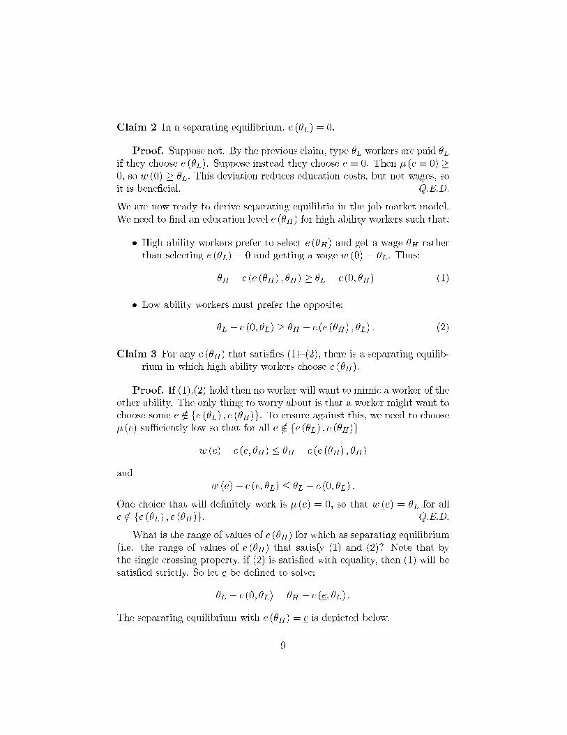
Claim 2 In a separating equilibrium, e (θL) = 0.

Proof. Suppose not. By the previous claim, type θL workers are paid θLif they choose e (θL). Suppose instead they choose e = 0. Then µ (e = 0) ≥0, so w (0) ≥ θL. This deviation reduces education costs, but not wages, soit is beneficial. Q.E.D.

We are now ready to derive separating equilibria in the job market model.We need to find an education level e (θH) for high ability workers such that:

• High ability workers prefer to select e (θH) and get a wage θH ratherthan selecting e (θL) = 0 and getting a wage w (0) = θL. Thus:

θH − c (e (θH) , θH) ≥ θL − c (0, θH) (1)

• Low ability workers must prefer the opposite:

θL − c (0, θL) ≥ θH − c (e (θH) , θL) . (2)

Claim 3 For any e (θH) that satisfies (1)—(2), there is a separating equilib-rium in which high ability workers choose e (θH).

Proof. If (1),(2) hold then no worker will want to mimic a worker of theother ability. The only thing to worry about is that a worker might want tochoose some e /∈ {e (θL) , e (θH)}. To ensure against this, we need to chooseµ (e) sufficiently low so that for all e /∈ {e (θL) , e (θH)}

w (e)− c (e, θH) ≤ θH − c (e (θH) , θH)

andw (e)− c (e, θL) ≤ θL − c (0, θL) .

One choice that will definitely work is µ (e) = 0, so that w (e) = θL for alle /∈ {e (θL) , e (θH)}. Q.E.D.

What is the range of values of e (θH) for which as separating equilibrium(i.e. the range of values of e (θH) that satisfy (1) and (2)? Note that bythe single crossing property, if (2) is satisfied with equality, then (1) will besatisfied strictly. So let e be defined to solve:

θL − c (0, θL) = θH − c (e, θL) .

The separating equilibrium with e (θH) = e is depicted below.

9

e

w

IL IH

θH

θL

w(e)

e

The single-crossing property also implies that if (1) is satisfied withequality, then (2) will be satisfied strictly. Define e to solve:

θH − c (e, θH) = θL − c (0, θH) .

The separating equilibrium with e (θH) = e is depicted below.

e

w

IL IH

θH

θL

w(e)

e e(θH)

In fact, there is separating equilibrium for any e ∈ [e, e], but not for anye outside of this interval.

Remark 2 Note the important role played by the single crossing property.This is what allows high ability workers to choose a positive education levelthat is costly, but less costly for them than it would be for low ability workers.It is this differential cost that allows separation.

10

Pooling Equilibria. In a pooling equilibrium, every worker chooses thesame education level eP with probability one. Therefore, the labor marketmust have beliefs µ(eP ) = λ in equilibrium, and thus:

w(eP)= λθH + (1− λ) θL = θE .

Now, let e be defined so that:

θE − c (e, θL) = θL − c (0, θL) .

That is, e is chosen so that a low ability worker is just indifferent to acquiringeducation e and being paid θE , and acquiring no education and being paidθL.

Proposition 1 For any eP ∈ [0, e], there is a pooling equilibrium in which

all workers choose eP for certain.

Proof. Let eP ∈ [0, e] be given. Suppose that µ(eP ) = λ and thatµ (e) = 0 for all e �= eP , with wages given accordingly. Then w (e) < w(eP ),so clearly no worker wants to deviate to e > eP . Moreover, θL workers prefereP to any e < eP by definition of e. And since θL workers prefer eP to anylower e, so must θH workers (by the single crossing property).

There are a few general points to make about the signalling model. First,in the separating equilibrium, education does not increase productivity, butit does reveal information. Thus it is correlated with wages in equilib-rium. In the pooling equilibrium, education neither increases productivitynor reveals information. Nevertheless, workers may incur education costs inequilibrium because there is a wage penalty for doing something unexpected(i.e. not becoming educated). Thus pooling pooling equilibria with positiveeducation levels are very inefficient.

A special feature of the model is that education is not productive at all.We could, however, generalize the model to let the worker’s productivity bea function of both ability and education: θ + e, for example. Things wouldwork out in a similar manner – with the key idea being that signallingwould lead workers to invest more in education than is efficient.

2.3 The Intuitive Criterion

What can be said about the vast multiplicity of equilibria in the signallingmodel? Cho and Kreps (1987) argue that some equilibria are less appealingthan others. We now consider their “intuitive criterion” for eliminatingsignalling equilibria.

11

Definition 7 Let BR (T, a1) denote the set of player 2’s best responses if

player 1 has chosen a1 and player 2’s beliefs have support in T ⊂ Θ :

BR (T, a1) = ∪µ∈∆(T ) arg maxa2∈A2

∑u2 (a1, a2, θ)µ (θ)

Definition 8 A PBE s∗ of G fails the intuitive criterion if there exists

a1 ∈ A1, θ′ ∈ Θ and J ⊂ Θ such that

1. u1 (s∗, θ) > maxa2∈BR(Θ,a1) u1 (a1, a2, θ) for all θ ∈ J

2. u1 (s∗, θ) < mina2∈BR(Θ/J,a1) u2

(a1, a2, θ

′)

Condition (1) implies that types in J would never try to play a1 sinceeven if they could convince player 2 that they were a particular type, theywould do worse. Condition (2) implies that type θ′ definitely does better byplaying a1 rather than the equilibrium so long as she can convince player 2that her type is not in J .

Proposition 2 In the job market signalling model, any pooling equilibrium

fails the intuitive criterion.

Proof. Consider a pooling equilibrium with some education level eP .Then we look for a education level e that satisfies:

θE − c(eP , θL

)> θH − c (e, θL)

andθE − c

(eP , θH

)< θH − c (e, θH) .

The Figure below show how to identify e.

e

w

IL

IH

θH

θL

w(e)

eP e

θE

I’H

12

Tracing the indifference curves through(w = θE , eP

), we look for the

education level that puts the low ability type on the same indifference curvewhen w = θH . A slight increase to e will then suffice – at (w = θH , e), thelow ability type will be on a lower indifference curve than at

(θE , eP

), while

the high ability type is on a higher indifference curve. Q.E.D.

It is also possible to show that of the separating equilibria derived above,only the most efficient – the separating equilibrium where the high abilitycost type gets education e survives the intuitive criterion. This is typical ofthe intuitive criterion – in models with separating equilibria, it selects themost efficient. You are asked to work out another example on the problemset.

3 Cheap Talk

In signalling models, a player uses costly action to communicate informationabout his type. In some situations, however, effective costly signals may notbe available. This raises the question of whether a player could crediblycommunicate information about his type simply through a costless processof communication. It is this possibility that we now explore.

3.1 The Model

The basic model of cheap talk is exactly like the signalling model, only player1’s action is a message that has no direct effect on payoffs.

Stage 0 Nature chooses type θ ∈ Θ of player 1 from a distribution p.

Stage 1 Player 1 observes θ and chooses m ∈M .

Stage 2 Player 2 observes m and chooses a ∈ A.

Payoffs u1 (a, θ) and u2 (a, θ).

We sometimes call player 1 the “sender” and player 2 the “receiver”.We are interested in studying perfect bayesian equilibria of this game. Thebasic question is whether player 1’s message will ever convey meaning inequilibrium.

13

3.2 Basic Observations

1. Cheap talk doesn’t work if different types of senders have the samepreferences over actions.

Example Consider a job market game where instead of going to schoolplayers just say “I’m high θ” or “I’m low θ”. This game has payoffs:

aL aM aHθ = L 1, 1 2, 0 3,−2θ = H 1,−2 2, 0 3, 1

Claim. In this game there are no separating PBE.

Proof. Consider a candidate PBEwhere s1 (θ = L) =m and s1 (θ = H) =m′ with m �=m′. By Bayes Rule’:

µ2 (L|m) = 1 ⇒ a (m) = aL

and so:µ2

(L|m′

)= 0 ⇒ a

(m′

)= aH

But then when θ = L, player 1 would like to deviate since

u1 (a (m) , L) = 1 < 3 = u2(a(m′

), L

)

so this cannot be a PBE. Q.E.D.

2. Cheap talk doesn’t work if different types of senders have completelyopposed preferences over actions.

Example Suppose that Vince McMahon (player 2) is thinking about hiringMike Tyson (player 1) as a WWF wrestler. In the Mike Tyson game,Mike can be either Normal or Crazy.

Θ = {Normal, Crazy}

Mike wants the job if he is normal, but not is he is crazy. On theother hand, Vince wants to hire Mike if and only if Mike is crazy. Wewrite the payoffs for Mike and Vince as follows:

Hire Don’t Hireθ = N 2,−2 0, 0θ = C −2, 2 0, 0

14

Prior to Vince’s decision, Mike holds a press conference to announcehis state of mind.

Claim. In this game, there are no separating PBE.

Proof. Suppose that s1 (N) = m, s2 (C) = m′ with m �= m′. ByBayes’ Rule:

µ2 (N |m) = 1 ⇒ a (m) = D

µ2(N |m′

)= 0 ⇒ a

(m′

)= H

It follows that both types of Tyson want to switch messages:

u1 (a (m) ,N) = 0 < 2 = u1(a(m′

),N

)

u1 (a (m) , C) = 0 > −2 = u1(a(m′

), C

).

which means this cannot be an equilibrium. Q.E.D.

3. Cheap talk can work great in coordination games.

Example Consider a version of the “meeting place in New York” gamewhere player 1 is already there and is not allowed to move. Supposethat player 1’s “type” is his location in New York.

Θ = {Grand Central Station, Empire State Building} .

Player 1 knows θ and calls player 2 on the phone. Player 2 listens andthen chooses {G,E}. Payoffs are given by:

G Eθ = G 1, 1 0, 0θ = E 0, 0 1, 1

This game has a separating equilibrium:

s1 (G) = m s1 (E) =m′

µ2 (θ = G|m) = 1 µ2(θ = G|m′

)= 0

a2 (m) = G a2(m′

)= E

Remark 3 Note that this last example also has a pooling or “babbling” equi-librium, where player 1 always saysm (orm′ or randomizes over all elementsof M), and player 2 does not update her beliefs at all.

15

3.3 A Richer Model

We now tackle a richer model of cheap talk where the possibilities for com-munication are more interesting. We assume that θ is uniformly distributedon the interval [0, 1]. Let player 2’s action be denoted a ∈ R. We assumethat player 2 (the receiver) has payoffs u2 (a, θ) = − (a− θ)2, while player 1(the sender) has payoffs u1 (a, θ) = − (a− θ − c)2.

Player 2’s optimal action is to choose a = θ, while player 1’s is to choosea = θ + c. Importantly, preferences are congruent in the sense that bothlike to take higher actions when the state is higher. However, player 1 issystematically biased by an amount c.

We investigate different types of perfect bayesian equilibria.

Babbling Equilibrium. Player 1 uses each message m ∈ M with equalprobability regardless of θ. Player 2 assigns a uniform belief to all valuesθ ∈ [0, 1] regardless of the message. She then chooses that action a = 1/2.

Clearly player 1 cannot deviate profitably given Player 2’s beliefs. Simi-larly, Player 2’s action is optimal given her beliefs. Finally, Player 2’s beliefsare consistent with Bayes’ Rule.

A Two Message Equilibrium. Let’s try to construct an equilibriumwhere Player 1 uses two messages, m1 and m2. Let a (m) denote player 2’saction in response to message m. If the equilibrium conveys information, itmust be the case that a (m1) �= a (m2). Assume without loss of generalitythat a (m1) < a (m2).

Claim 1 In a two message equilibrium, player 1 uses a threshold strategy,choosing the message m1 whenever θ ∈ [0, θ∗) and m2 whenever θ ∈(θ∗, 1], with θ∗ indifferent (and choosing either).

Proof. To prove this note that player 1’s payoff are as follows:

Payoff to m1 : − (a (m1)− θ − c)2

Payoff to m2 : − (a (m2)− θ − c)2

So the incremental gain to choosing message m2 versus m1 is:

∆(θ) = − (a (m2)− θ − c)2 + (a (m1)− θ − c)2

This is increasing in θ. Thus, it follows that if type θ prefers m2 to m1, sowill every type θ′ > θ. This gives a threshold characterization with θ∗ beingthe type that is just indifferent. Q.E.D.

16

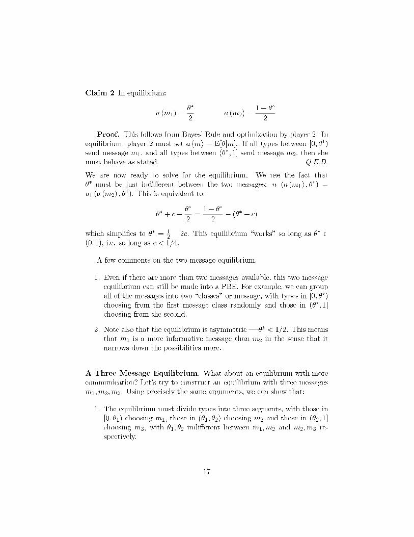
Claim 2 In equilibrium:

a (m1) =θ∗

2a (m2) =

1 + θ∗

2

Proof. This follows from Bayes’ Rule and optimization by player 2. Inequilibrium, player 2 must set a (m) = E[θ|m]. If all types between [0, θ∗)send message m1, and all types between (θ∗, 1] send message m2, then shemust behave as stated. Q.E.D.

We are now ready to solve for the equilibrium. We use the fact thatθ∗ must be just indifferent between the two messages: u1 (a (m1) , θ

∗) =u1 (a (m2) , θ

∗). This is equivalent to:

θ∗ + c−θ∗

2=

1 + θ∗

2− (θ∗ + c)

which simplifies to θ∗ = 1

2− 2c. This equilibrium “works” so long as θ∗ ∈

(0, 1), i.e. so long as c < 1/4.

A few comments on the two message equilibrium.

1. Even if there are more than two messages available, this two messageequilibrium can still be made into a PBE. For example, we can groupall of the messages into two “classes” or message, with types in [0, θ∗)choosing from the first message class randomly and those in (θ∗, 1]choosing from the second.

2. Note also that the equilibrium is asymmetric – θ∗ < 1/2. This meansthat m1 is a more informative message than m2 in the sense that itnarrows down the possibilities more.

A Three Message Equilibrium. What about an equilibrium with morecommunication? Let’s try to construct an equilibrium with three messagesm1,m2,m3. Using precisely the same arguments, we can show that:

1. The equilibrium must divide types into three segments, with those in[0, θ1) choosing m1, those in (θ1, θ2) choosing m2 and those in (θ2, 1]choosing m3, with θ1, θ2 indifferent between m1,m2 and m2,m3 re-spectively.

17

2. In equilibrium, player two must use:

a (m1) =θ12

a (m2) =θ1 + θ2

2a (m3) =

1 + θ22

,

i.e. she must set a (m) = E[θ|m] for m =m1,m2,m3.

3. Finally, we have two indifference conditions. Type θ1 must be indif-ferent between m1 and m2 :

(θ1 + c)−θ12

=θ1 + θ2

2− (θ1 + c)

and type θ2 must be indifferent between m2 and m3 :

(θ2 + c)−θ1 + θ2

2=

1 + θ22

− (θ2 + c) .

Solving these two equations implies that θ1 =1

3− 4c and θ2 =

2

3− 4c.

This “works” as an equilibrium provided that θ1 > 0, or in other words ifc < 1

12. So if there is a three message equilibrium, there is also a two message

equilibrium and a babbling equilibrium. Note also that the degree of biasmust be smaller to have more communication (three messages in equilibriumas opposed to just two).

Arbitrary Message Equilibrium. It is possible to show that there arealso 4,5,6,...,T message equilibria for some T which depends on c. In general,however, there is no fully separating (infinite message) equilibrium. Thereason is that if messages were fully informative, then type θ would sendthe report corresponding to type θ + c and achieve a better outcome (i.e.the action a = θ + c rather than the action θ). Thus in any equilibrium,there is some loss of information. And moreover, the loss of informationis directly related to the bias of the informed party. These results wereoriginally worked out in a paper by Crawford and Sobel (1982).

4 Models of Reputation

Some of the most striking applications of incomplete information are tomodels of reputation. We will consider two kinds of reputation models.

• In the first model, we consider a long-run player who plays againsta sequence of short-run playerss We find is that if short-run playersentertain the possibility that the long-run player is irrational in a par-ticular way, the long-run player may be able to build a reputation thatworks to his advantage.

18

• In the second model, we consider two long-run players. We find thatagain the slight possibility of irrationality changes the equilibriumgreatly, for instance, allowing cooperation in the finitely repeated pris-oners’ dilemma.

4.1 Building a Reputation for Toughness

We start by considering the following entry game.

Firm 2

Firm 1

InOut

Fight Accomodate

-1, -1 0, 1

2, 0

We consider a situation where this game is played T times. In each case,Player 1 is the same, but he faces a succession of Player 2s. Thus Player1’s objective is to maximize the undiscounted sum of his payoffs for all Tperiods, while each Player 2 wants to maximize her payoffs in the presentperiod.

As an example of this type of situation, think of Player 1 as Microsoft,fending off a succession of lawsuits accusing it of anti-competitive behav-ior. There are a succession of small firms who feel they have a case againstMicrosoft and have to decide whether to launch a court battle or not. Mi-crosoft then decides whether to settle (accomodate) or to fight tooth andnail (fight). The question is whether Microsoft might be able to fight someearly lawsuits, and thus “build a reputation” for fighting so that later firmswill not challenge it.

Proposition 3 In the T -period complete information game, there is a uniqueSPE in which Player 1 accomodates in all periods and all entrants enter.

Proof. Use backward induction. Q.E.D.

This result points to the strength of subgame perfection in complete infor-mation games. (Recall the centipede game or the Enron speculation game.)

19

Even if Microsoft is going to face a large number of challengers, it cannotbuild a reputation for being a fighter in this setting.

To incorporate reputation in this model, we relax the assumption thatPlayer 1 is necessarily rational, and suppose instead that with small prob-ability Player 1 actually enjoys fighting. To do this, suppose that Player 1has two possible types:

θ1 ∈ {Crazy, Normal}

Player 1 is crazy with probability q. For a crazy type, we assume that Fightis a dominant strategy – a Crazy type of player 1 will fight in every periodthat an opponent enters.

Even in the T = 1 period game, this aspect of craziness may be enoughto deter entry.

Proposition 4 In the T = 1 period game with incomplete information:

1. If q > 1/2, the unique PBE has player 2 play Out.

2. If q < 1/2, the unique PBE has player 2 play In.

Proof. This also can be solved by backward induction. Q.E.D.

However, the Normal player 1 behaves normally by accomodating theunique PBE. Things get more interesting when we go to the T = 2periodgame.

Proposition 5 In the T = 2 period game with incomplete information:

1. If q > 1/2, the unique PBE has the form:

Period 1: Player 2 stays OutPlayer 1 Fights

Period 2: Player 2 stays Out (unless he has seen Player 1 Accomodate)Player 1 Accomodates

2. If q < 1/2, the unique PBE has the form:

Period 1: Player 2 stays Out if q > 1/4 and Enters if q < 1/4.Player 1 Fights with Prob q/ (1− q) if 2 enters

Period 2: Player 2 enters (unless he has seen Player 1 Fightin which case he randomizes 1

2In+ 1

2Out.

Player 1 Accomodates

20

Remark 4 The strategies for Player 1 are for the case when he is Normal.If he is Crazy, he always Fights.

We consider the two cases in turn.Proof of (a): q > 1/2.

1. Because a Crazy Player 1 always plays Fight, Player 2 will not enterif she believes the probability that Player 1 is Crazy is greater than1/2. Consequently, Player 2 certainly will not enter in the first period.Moreoever, if there is no first period entry, Player 2 will continue tobelieve in the second period that Player 1 is Crazy with probabilityq > 1/2. Consequently, she will not enter in the second period either.

We conclude that Player 2’s equilibrium strategy is not to enter in either thefirst or the second period. However, we still need to describe what happensoff the equilibrium path – i.e. when Player 2 does enter in the first period.

2. If Player 2 enters in the first period and Player 1 responds by Accomo-dating, this reveals that Player 1 is Normal. So in the second period,Player 2 will find it optimal to enter, and Player 1 will find it optimalto respond by Accomodating.

3. If Player 2 enters in the first period and Player 1 responds by Fighting,then regardless of the Normal Player 1’s strategy, Player 2 must believeat the beginning of the second period that Player 1 is crazy withprobability at least q. From Bayes’ rule:

Pr [Crazy|a1 = Fight ] =q

q + (1− q) · Pr [Normal P1 Fights]≥ q.

It follows that in the second period, Player 2 will find it optimal notto enter, even though in the event of entry a Normal Player 1 wouldAccomodate.

We conclude that a Normal Player 1 would always Accomodate in the secondperiod, but that following entry in the first period, Player 2 would enter inthe second if and only if she saw Player 1 Accomodate in the first. Finally,we need to consider what a Normal Player 1 would do in the first periodshould Player 2 enter.

4. If Player 2 enters in the first period, then by playing Fight a NormalPlayer 1 can deter second-period entry. In particular, playing Fight

21

gives a payoff of −1 + 2 = 1. On the other hand, Accomodating givesa payoff of 0 today and encourages entry leading to 0 tomorrow. SoPlayer 1 will optimally Fight should Player 2 enter in period 1.

This completely describes the perfect bayesian equilibrium if q > 1/2.Q.E.D.

Proof of (a): q < 1/2.We start by considering what happens if Player 2 does not enter in the

first period.

1. If Player 2 does not enter in the first period, then there is no learningabout player 1’s type. In the second period, we have a one-shot gamewith probability q < 1/2 that Player 1 is Crazy. Consequently, Player 2will enter in the second period and a Normal Player 1 will accomodate.

Now consider what happens if Player 2 enters in the first period.

2. It cannot be a PBE for Player 1 to fight with probability 1 in thefirst period. If it was, then Player 2 would not update when she sawPlayer 1 fight and thus would enter in the second period regardlessof whether or nor Player 1 fought or accomodated in the first period.Consequently, a Normal Player 1 would do better to accomodate inthe first period.

3. It also cannot be a PBE for Player 1 to accomodate with probability 1in the first period. If it was, then fighting would perfectly signal crazi-ness. After seeing Fight, Player 2 would not enter the second period.But then the payoff to Fighting in the first period for Normal Player1 would be −1 + 2 = 1, greater than the payoff 0 to accomodating.

We conclude that the PBE must have Player 1 randomize in the first period.For Player 1 to be willing to randomize, he must be indifferent to playingFight and Accomodate in the first period. This means that:

0 = −1 + 2 · Pr [2 Out in period 2|a1 = Fight ]

+0 · Pr [2 Enters in period 2|a1 = Fight] .

For this to happen, it must be that:

Pr [2 Out in period 2| a1 = Fight ] =1

2.

22

We conclude from this that the PBE must have Player 2 randomize in thesecond period after seeing Fight in the first.

For Player 2 to be willing to randomize in the second period after seeingFight in the first, it must be that:

Pr [Crazy|a1 = Fight ] =1

2.

In equilibrium, this belief will be obtained through Bayes’ updating:

Pr [Crazy| a1 = Fight ] =q

q + (1− q) · Pr [Normal P1 Fights in Period 1].

Combining these requirement, we find that the Normal Player 1 must fightentry in period 1 with probability q/ (1− q).

At this point, we have determined (a) what Normal Player 1 must doin period 1 if Player 2 enters, and (b) what Player 2 will do after (i) notentering in period 1, (ii) entering in period 1 and seeing Fight, and (iii)entering in Period 1 and seeing Accomodate.

The remaining question is whether Player 2 will enter in the first period.Her payoff to entering is:

−

(q + (1− q) ·

q

1− q

)+ (1− q) ·

1− 2q

1− q= 1− 4q.

while staying out gives zero We conclude that Player 2 will optimally enterin the first period if q < 1/4, and will optimally stay out in the first periodif q > 1/4. Q.E.D.

The general T -period version of this model has also been studied. Itturns out that if T is large, then even if q is quite small, the Normal typeof Player 1 will be able to mimic the Crazy type and obtain a large periodperiod payoff. Remarkably, as T → ∞, the Normal player’s average payoffper-period approaches 2 (which is the highest payoff that player 1 could getby committing to a strategy in advance – i.e. his “Stackelberg” payoff). Inthis sense, the slight chance that a player is crazy may allow that player todo very well in equilibrium.

4.2 Cooperation in the Finitely Repeated Prisoners’ Dilemma

In the above example, the long-run Player 1 was able to build a reputationto his own advantage. Reputation can also play a powerful role in situations

23

where players may be able to constructively mislead others about their ob-jectives. To see how this works, we consider Kreps, Milgrom, Roberts, andWilson’s (1982) treatment of the finitely repeated prisoners’ dilemma.

The stage game is the standard prisoners’ dilemma.

C DC 1, 1 −1, 2D 2,−1 0, 0

We assume the game is repeated T times with no discounting, with bothplayer 1 and 2 being long-run players. Recall that if both players are max-imizing their payoffs and there is complete information, then backward in-duction tells us that (D,D) will be played in every period of the uniquesubgame perfect equilibrium.

To add reputation, we imagine that player 2 is either “crazy” with prob-ability q or “normal” with probability 1 − q. A normal player maximizeshis expected payoff in the standard way, but a crazy player mechanicallyplays the Grim Trigger strategy. That is a crazy Player 2 plays C so long asPlayer 1 has never played D, and plays D forever once Player 1 has playedD for the first time.

If this this incomplete information game is played once, both Player 1and the Normal Player 2 have a dominant strategy, which is to play D.However, if the game is played more than once, the possibility that Player 2might be crazy gives Player 1 some incentive to play C in the early rounds.More subtle is the fact that it also gives Player 2 an incentive to play C –by doing so Player 2 can potentially convey the impression that he really iscrazy.

Proposition 6 In the T = 2 period model, the normal Player 2 alwaysplays D, while Player 1 plays C in the first period if q > 1/2.

Proof. In the second period, both the Normal Player 2 and Player 1 willclearly want to choose D regardless of what happened in the first period andregardless of Player 1’s beliefs about Player 2’s type. The Crazy Player 2will play C if Player 1 played C in the first period and D if Player 1 playedD.

In the first period, the Normal Player 2will certainly play D since re-gardless of what she plays she expects Player 1 to play D in the last peiriod.The Crazy Player 2 will play C. Now consider Player 1. She has payoffs:

Payoff to C : q − (1− q) + q · 2 = 4q − 1

Payoff to D : 2q

24

Thus Player 1 optimally plays C in the first period if q > 1/2 and optimallyplays D if q < 1/2. Q.E.D.

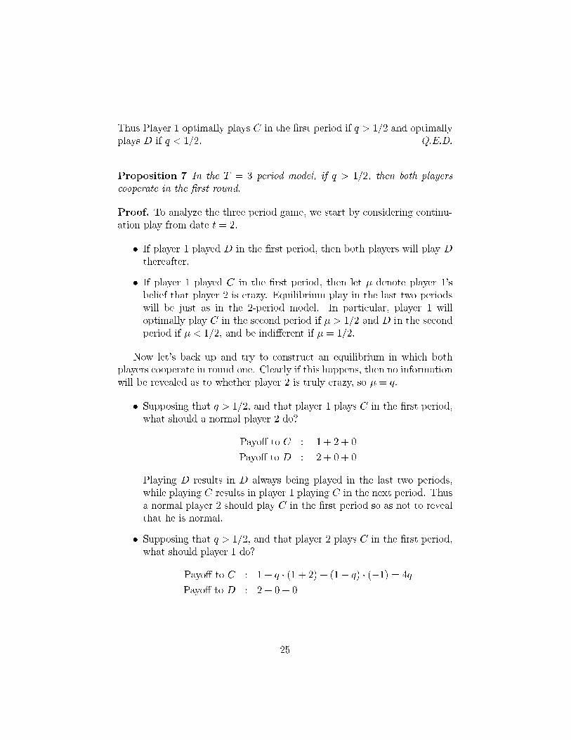
Proposition 7 In the T = 3 period model, if q > 1/2, then both playerscooperate in the first round.

Proof. To analyze the three period game, we start by considering continu-ation play from date t = 2.

• If player 1 played D in the first period, then both players will play Dthereafter.

• If player 1 played C in the first period, then let µ denote player 1’sbelief that player 2 is crazy. Equilibrium play in the last two periodswill be just as in the 2-period model. In particular, player 1 willoptimally play C in the second period if µ > 1/2 and D in the secondperiod if µ < 1/2, and be indifferent if µ = 1/2.

Now let’s back up and try to construct an equilibrium in which bothplayers cooperate in round one. Clearly if this happens, then no informationwill be revealed as to whether player 2 is truly crazy, so µ = q.

• Supposing that q > 1/2, and that player 1 plays C in the first period,what should a normal player 2 do?

Payoff to C : 1 + 2 + 0

Payoff to D : 2 + 0 + 0

Playing D results in D always being played in the last two periods,while playing C results in player 1 playing C in the next period. Thusa normal player 2 should play C in the first period so as not to revealthat he is normal.

• Supposing that q > 1/2, and that player 2 plays C in the first period,what should player 1 do?

Payoff to C : 1 + q · (1 + 2) + (1− q) · (−1) = 4q

Payoff to D : 2 + 0 + 0

25

So player 1 should also play C in the first period. Q.E.D.

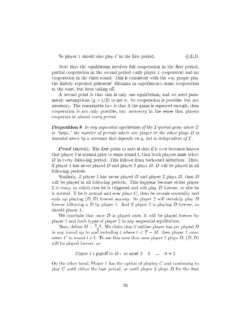
Note that the equilibrium involves full cooperation in the first period,partial cooperation in the second period (only player 1 cooperates) and nocooperation in the third round. This is consistent with the way people playthe finitely repeated prisoners’ dilemma in experiments: some cooperationat the start, but hten tailing off.

A second point is that this is only one equilibrium, and we need para-metric assumptions (q > 1/2) to get it. So cooperation is possible, but notnecessary. The remarkable fact is that if the game is repeated enough, thencooperation is not only possible, but necessary in the sense that playerscooperate in almost every period.

Proposition 8 In any sequential equilibrium of the T -period game where Tis “large,” the number of periods where one player or the other plays D isbounded above by a constant that depends on q, but is independent of T .

Proof (sketch). The first point to note is that if it ever becomes knownthat player 2 is normal prior to some round t, then both players must selectD in every following period. This follows from backward induction. Thus,if player 1 has never played D and player 2 plays D, D will be played in allfollowing periods.

Similarly, if player 1 has never played D and player 2 plays D, then Dwill be played in all following periods. This happens because either player2 is crazy, in which case he is triggered and will play D forever, or else heis normal. If he is normal and ever plays C, then he reveals normality andends up playing (D,D) forever anyway. So player 2 will certainly play Dforever following a D by player 1. And if player 2 is playing D forever, soshould player 1.

We conclude that once D is played once, it will be played forever byplayer 1 and both types of player 2 in any sequential equilibrium.

Next, define M = 3−q

q. We claim that if neither player has yet played D

in any round up to and including t where t < T −M , then player 1 mustselect C in round t+1. To see this note that once player 1 plays D, (D,D)will be played forever, so

Player 1’s payoff to D : at most 2 + 0 + ...+ 0 = 2

On the other hand, Player 1 has the option of playing C and continuing toplay C until either the last period, or until player 2 plays D for the first

26

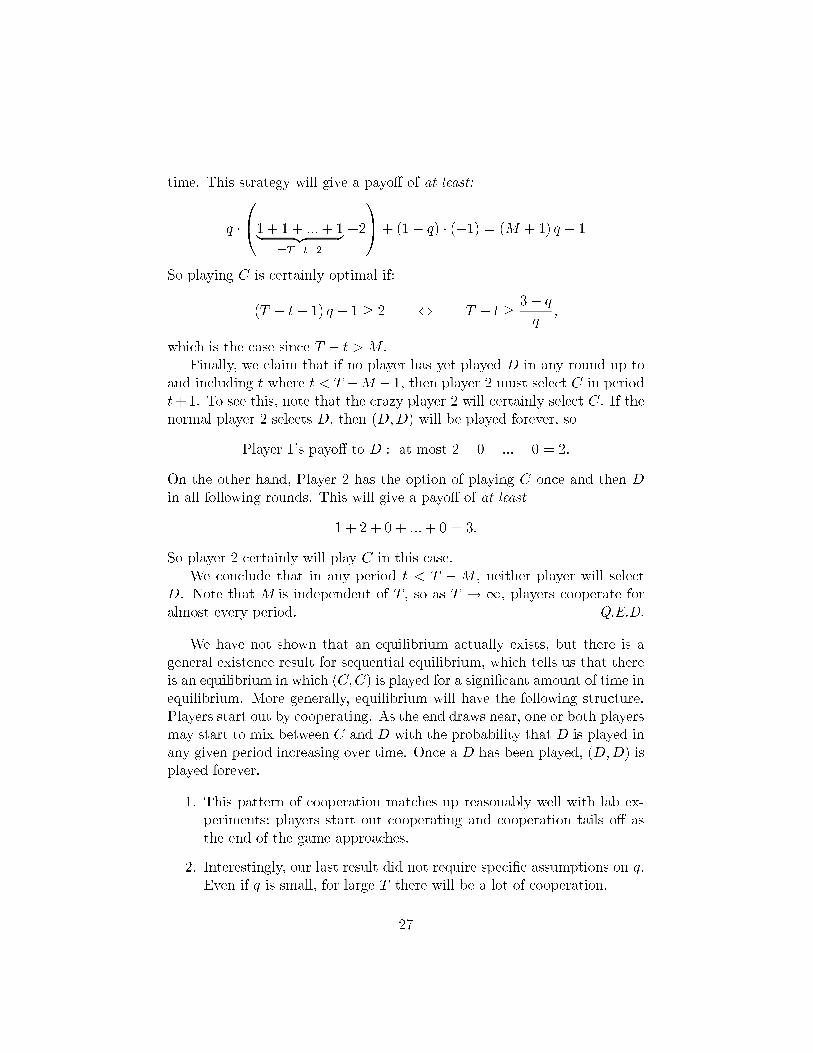
time. This strategy will give a payoff of at least:

q ·

1 + 1 + ...+ 1︸ ︷︷ ︸

=T−t−2

+2

+ (1− q) · (−1) = (M + 1) q − 1

So playing C is certainly optimal if:

(T − t− 1) q − 1 ≥ 2 ⇔ T − t ≥3− q

q,

which is the case since T − t > M .Finally, we claim that if no player has yet played D in any round up to

and including t where t < T −M − 1, then player 2 must select C in periodt+1. To see this, note that the crazy player 2 will certainly select C. If thenormal player 2 selects D, then (D,D) will be played forever, so

Player 1’s payoff to D : at most 2 + 0 + ...+ 0 = 2.

On the other hand, Player 2 has the option of playing C once and then Din all following rounds. This will give a payoff of at least

1 + 2 + 0 + ...+ 0 = 3.

So player 2 certainly will play C in this case.We conclude that in any period t < T −M , neither player will select

D. Note that M is independent of T , so as T → ∞, players cooperate foralmost every period. Q.E.D.

We have not shown that an equilibrium actually exists, but there is ageneral existence result for sequential equilibrium, which tells us that thereis an equilibrium in which (C,C) is played for a significant amount of time inequilibrium. More generally, equilibrium will have the following structure.Players start out by cooperating. As the end draws near, one or both playersmay start to mix between C and D with the probability that D is played inany given period increasing over time. Once a D has been played, (D,D) isplayed forever.

1. This pattern of cooperation matches up reasonably well with lab ex-periments: players start out cooperating and cooperation tails off asthe end of the game approaches.

2. Interestingly, our last result did not require specific assumptions on q.Even if q is small, for large T there will be a lot of cooperation.

27

3. We relied heavily on a particular form of craziness to get this result.It turns out that if one allows for all conceivable forms of craziness,and if both players may be crazy, there is a folk theorem type result– anything can happen.

References

[1] Cho, I.K. and D. Kreps (1987) “Signalling Games and Stable Equilibria,”Quarterly Journal of Economics.

[2] Crawford, V. and J. Sobel (1982) “Strategic Information Transmission,”Econometrica.

[3] Kreps, D., P. Milgrom, J. Roberts and R. Wilson (1982) “Cooperation inthe Finitely Repeated Prisoners’ Dilemma,” Journal of Economic The-ory.

[4] Kreps, D. and R. Wilson (1982) “Sequential Equilibrium,” Economet-rica.

[5] Spence, M. (1974) Market Signalling, Harvard University Press.

28