DYNAMIC FLUID FLOW IN HETEROGENEOUSPOROUS MEDIA AND THROUGH A SINGLE

FRACTURE WITH ROUGH SURFACES

by

Xiaomin Zhao, C.H. Cheng, Xiaoming Tang*, and M. Nafi Toksoz

Earth Resources LaboratoryDepartment of Earth, Atmospheric, and Planetary Sciences

Massachusetts Institute of TechnologyCambridge, MA 02139

*NER Geoscience1100 Crown Colony Drive

Quincy, MA 02169

ABSTRACT

This study investigates the frequency-dependence of fluid flow in heterogeneous porousmedia using the theory of dynamic penneability and a finite-difference method. Givena penneability distribution, the dynamic penneability is applied locally to calculatethe frequency-dependence of fluid flow at each local point. An iterative AlternatingDirection Implicit finite-difference technique is applied to calculate the flow field in thefrequency domain. We compare the flow through a 2-D heterogeneous porous mediumand that through an equivalent homogeneous medium and find that the two mediado not behave equivalently as a function of frequency. At very low-frequencies, theheterogeneous medium is less conductive than the homogeneous medium, However, inthe transition region from quasi-static to dynamic regimes, the fonner medium becomesmore conductive than the latter medium, with the ratio of the fonner flow over the latterflow reaching a maximum in this region. The larger the scale, or the higher the degreeof the heterogeneity, the higher this maximum is. This finding is important for studyingthe interaction of a borehole stoneley wave with a heterogeneous porous fonnation.

The finite-difference technique is also applied to simulate frequency-dependent flowthrough a single fracture with rough surfaces. It is shown that the fiow exhibits strongfrequency-dependence even for small fractures with contacting surfaces. The amount offlow through the fracture is reduced by the surface roughness .

158 Zhao et al.

INTRODUCTION

Fluid flow in porous media is an important topic in the study of flow of oil or gas inpetroleum reservoirs. In many applications where the fluid driven (pressure) source istime invariant, steady-state (time-independent) flow is assumed and the flow can bemodeled for any distribution of heterogeneous porous media using a finite-differencetechnique (Zhao and Toksoz, 1991). When the fluid driven source changes moderatelywith time, such as the pressure transient tests in a borehole (Melville et aI, 1991) andin laboratory measurements (Brace et al, 1968; Kamath et al., 1990; Bernabe, 1991),fluid flow can be modeled as a diffusion process in which the fluid transport propertiessuch as permeability are still regarded as independent of time (or frequency) (Zhao andToksoz, this volume). Moreover, in applications related to wave propagation, such asvertical seismic profiling and acoustic logging, fluid flow associated with the pressuredisturbance set up by seismic wave propagation is dynamic in nature and may stronglydepend on frequency. In fact, in these situations, the frequency-dependent flow becomesthe Biot's slow wave (Biot, 1956a,b) in a porous medium.

To characterize the frequency-dependent fluid transport property, Johnson et al.(1987) developed the theory of dynamic permeability. Applying the concept of dynamicpermeability to the problem of acoustic logging in permeable porous formations, Tanget al. (1991) showed that the dynamic permeability captures the frequency-dependentbehavior of Biot's slow wave and correctly predicts the effects of formation permeabilityon borehole Stoneley waves. The theory of dynamic permeability is formuiated assum­ing the homogeneity of the porous medium. The natural geological medium, however,contains heterogeneities of various scales. It would be interesting to apply the dynamicpermeability to the heterogeneous porous media to study the overall behavior of fluidflow through the media. In this study, we will model the dynamic fluid flow in the het­erogeneous porous media using the theory of dynamic permeability. A finite-differencemethod will be developed to model the effects of heterogeneities.

A problem that has attracted much research interest is fluid flow through a rough­walled fracture or joint. Brown (1987, 1989) and Zimmerman et al. (1991) have modeledthe steady-state fluid flow through the fracture and showed that the roughness of thefracture surfaces significantly affects the fluid flow when the surfaces are in contact. Inthe characterization of borehole fractures using acoustic logging (Paillet et aI., 1989;Hornby et aI., 1989), the response of the fracture to the dynamic pressure set up by thelogging waves is important for characterizing the fracture permeability. In this situation,fluid flow in fractures is dynamic in nature. Tang and Cheng (1989) have studied thedynamic flow through a plane fracture bounded by two parallel walls. Natural fracturesurfaces, however, exhibit roughness (Brown, 1987). It is important to understand theeffects of surface roughness on the dynamic fluid flow in order to correctly model thedynamic response of natural fractures to borehole acoustic waves. Tang et al. (1991)

(

Dynamic Fluid Flow 159

have shown that the theory of dynamic penneability, when applied to the parallel-wallfracture, is equivalent to the theory of fracture dynamic conductivity. Therefore, ifwe assume that the dynamic penneability for a parallel-wall fracture holds locally in afracture, then we can use the finite-difference code developed for heterogeneous porousmedia to model the dynamic flow in a rough-walled fracture.

In the following, we first discuss the theory of dynamic penneability and governingequations for the dynamic fluid fiow. Then we develop a finite-difference technique tosolve the flow equation in the frequency domain. Finally, we apply the finite-differencetechnique to study the dynamic flow through a single fracture with rough surfaces.

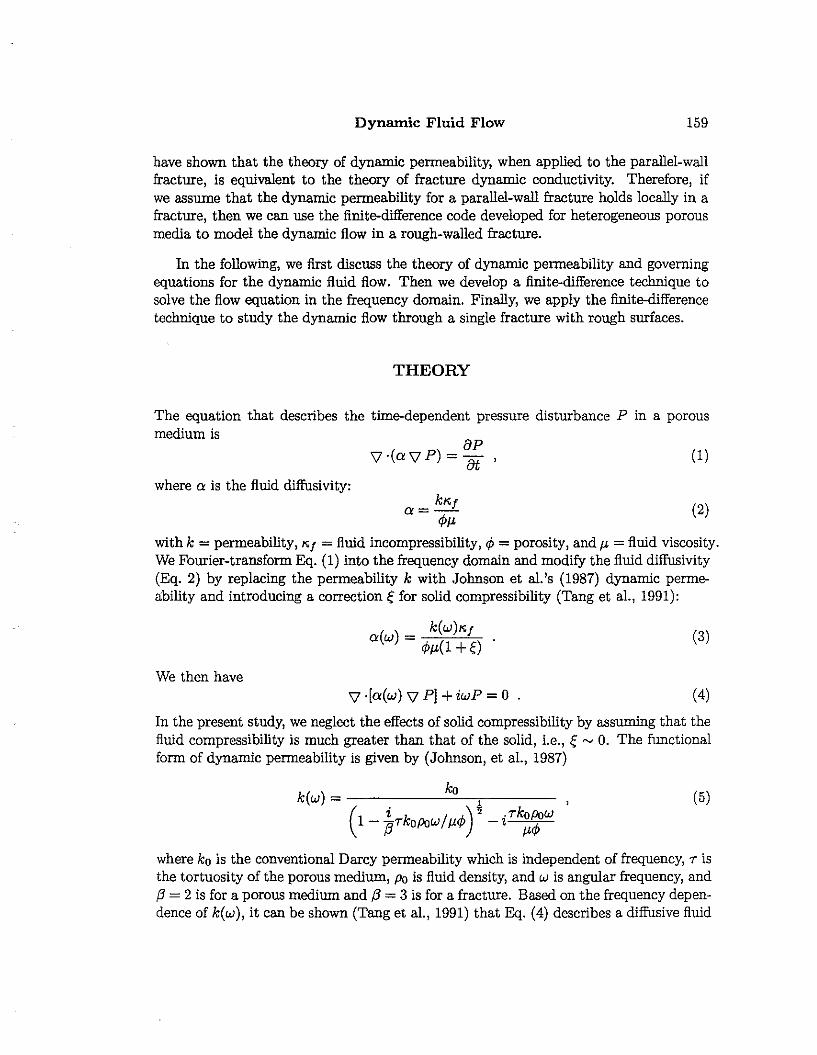
THEORY

The equation that describes the time-dependent pressure disturbance P in a porousmedium is

where a is the fluid diffusivity:

8P\1·(a \1 P) = 7ft ' (1)

kKfa = <P/1o (2)

with k = penneability, '"f = fluid incompressibility, <p = porosity, and /10 = fluid viscosity.We Fourier-transfonn Eq. (1) into the frequency domain and modify the fluid diffusivity(Eq. 2) by replacing the penneability k with Johnson et a1.'s (1987) dynamic penne­a:bility and introducing a correction efor solid compressibility (Tang et aI., 1991):

We then have

k(w)"'fa(w) = <p/1o(1 +e) (3)

(4)

(5)

In the present study, we neglect the effects of solid compressibility by assuming that thefluid compressibility is much greater than that of the solid, Le., e~ O. The functionalfonn of dynamic penneability is given by (Johnson, et aI., 1987)

kok~)= "

( i)"2 .TkoPoW1 - 73TkoPow/ /1o<P - ~ /1o<P

where ko is the conventional Darcy penneability which is independent of frequency, T isthe tortuosity of the porous medium, Po is fluid density, and w is anguiar frequency, andf3 = 2 is for a porous medium and f3 = 3 is for a fracture. Based on the frequency depen­dence of k(w), it can be shown (Tang et aI., 1991) that Eq. (4) describes a diffusive fluid

160 Zhao et al.

motion at low frequencies. At high frequencies, this motion becomes a propagationalwave. Therefore, Eq. (4) describes Biot's (1956a, b) slow wave in a porous medium withan incompressible solid matrix.

In this study, we will investigate the behavior of flow field over a distribution oftwo-dimensional (2-D) heterogeneities. To model the effects of the 2-D heterogeneitieson the fluid flow, we assign a 2-D distribution for the permeability ko, Le.,

ko = ko(x, y) . (6)

In this way, the dynamic permeability (Eq. 5) is not only a function of frequency, butalso a function of the spatial coordinates x and y. Because of the spatial variation (Ifko, flow in the heterogeneous porous medium may exhibit different characteristics atdifferent locations. For example, in regions where ko is small, the flow is dominatedby viscous diffusion, whereas in regions where ko is high, dynamic effects may becomesignificant and the flow becomes a propagational wave. Because k(w; x, V), as well asa(w), change spatially, Eq. (4) is written as

(

o [ OP] 0 [ ap].ax a(w;x,y) ax + ay a(w;x,y) By + tWP = 0 (7)

This equation, together with given boundary conditions, describes the fluid pressurefields in the 2-D heterogeneous porous medium for the given frequency w. We chooseto model the dynamic flow in the frequency domain because the dynamic permeabilityis defined as the function of frequency. This formulation allows us to study the flowbehavior over different frequency ranges.

FINITE-DIFFERENCE MODELING

For the finite-difference modeling, it is convenient to use dimensionless variables. Weintroduce the dimensionless permeability k' and spatial variables x' and y' as follows:

(

ko(x, y) = kmazk'(x, y)

x = Lxx'

y = Lyy'

O<k'<l

O<x'<l

O<y'<l

where km= is the maximum permeability over the region of interest, x' and y' are thedimensionless variables in x and y directions, respectively. For a square 2-D grid, weassume Lx = L y = L. We also introduce the characteristic frequency of the model

(8)

Dynamic Fluid Flow

The dimensionless frequency n is defined as

n=~wo

Using the dimensionless variables, Eq. (7) becomes

161

(9)

(10)

(14)

a [A( ") ap] a [( ") ap] .,...,ax' W; x ,y ax' + ay' A W; x ,y ay' + 2"P = 0 ,

where the dimensionless dynamic permeability is

A(w; x', y') = k'(a!'l~'} (11)(1 - ~rkm=k'(x', Y')~) - irkmaxk'(x', y')e:;

It is interesting to note that, because the spatial variation of k'(x',y') in A(w; x', y') iscoupled with the frequency w, A(w; x', 11) may have different distributions over the 2-Dgrids x' and y' at different frequencies.

Forward difference solution of Eq. (10) (which is a Helmholtz type equation) isunstable, especially for large n values where the dynamic effects become significant.This can be shown by analyzing a 1-D Helmholtz equation

d2pdx2 + >..2 P = 0 (12)

Substituting P = Poei.>.mx (where x = ml:l.x, m = 0, 1,2,"', M) into Eq. (12) and using

the forward difference ~~~ = Pm±l -:'2 + Pm 1, we have the following stability

equation:

(13)

This equation holds only when >..l:I.x is small. In Eq. (13), however, >.. = v'iIT is big whenn is big, Eq. (12) cannot have a solution unless l:I.x is exceedingly small. We thereforeuse an iterative procedure to solve Eq. (10). We write Eq. (10) as

a [A( ") ap] a [( ")ap] .,..., apax' w;x,y ax' + By' Aw;x,y ay' +2"P= at' ,

where t' is a dimensionless time. The steady-state solution of Eq. (14) will be thesolution of Eq. (10), and the solution of Eq. (14) will be unconditionally stable if wesolve it using the Alternating Direction Implicit (ADI) scheme (Ferziger, 1981; Zhaoand Toksiiz, this volume). Using the ADI method, the finite-difference form of Eq. (14)is

(15)

162 Zhao et aI.

where,

t:>.t'JL1 = 2 t:>.X,2

t:>.t'JL2 = 2t:>.y,2

and

Bi,; = VAi,; * A;+l,;

Ci,j = VAi,; * Ai,;+!

Here we use the geometric average for the mid-point between two adjacent grids becauseit gives a better approximation for the point when the values on the two adjacent gridsdiffer by orders. The boundary conditions are specified by assigning no-flow conditionsfor y' = 0 and 11 = 1, I.e.,

(

8P' =0811

at 11 = 0 and y' = 1 . (17)

The pressure spectrum Po(w) is assigned to the x' = 0 boundary. At x' = 1, thepressure is set to zero. With the algorithm, the solution is iterated with increasingn. The solution to Eq. (10) is obtained when the difference between p n+1 and pn issufficiently small.

TESTING THE FINITE-DIFFERENCE ALGORITHM

As a test of the numerical algorithm, we compare the finite-difference results with theresults from the analytical solution for a simple I-D case Eq. (12). For the I-D case, ifwe assign P!x=o = Po and P!x=L = 0, then the solution is

(

P(. ) _ R sin['\(L - x)]

w,x - a . 'L 'sm"

(18)

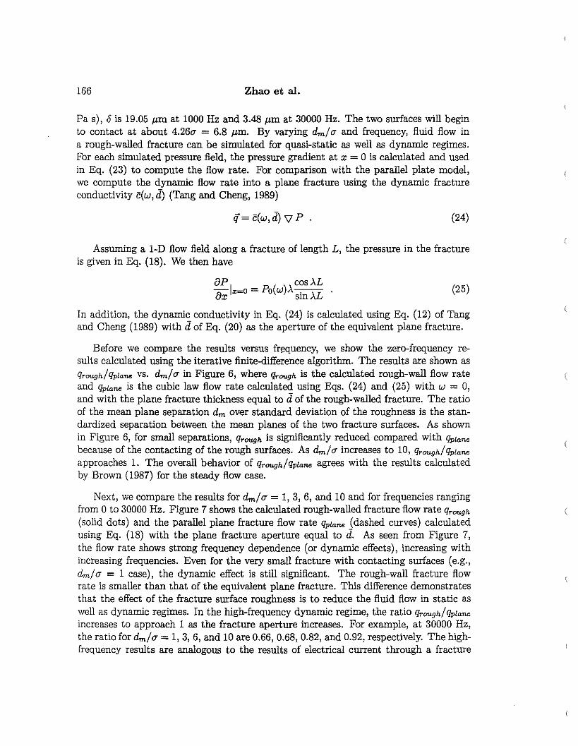
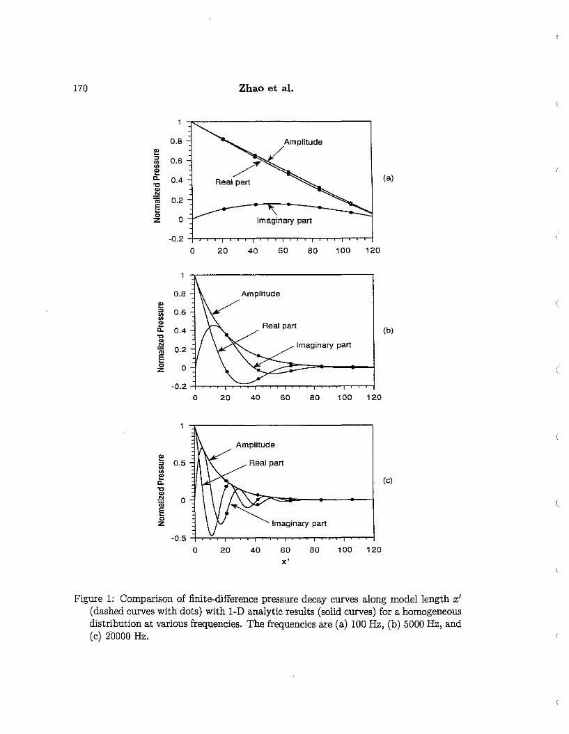
where ,\ now equals ki(~J~f for the dynamic flow problem. Figure 1 shows the com­

parison between the results of the finite-difference algorithm and Eq. (18), where theamplitude, the real and imaginary parts of the pressure spectrum P(w; x) are plotted.

Dynamic Fluid Flow 163

(19)

The parameters are ko = 1 Darcy, ¢ = 0.2, " = 2.25 X 109 Pa, and M= 1.14 X 103 Pa-s.For the finite-difference scheme, the pressure along the middle line y' = L /2 is used.The two results are in almost exact agreement (the no-flow boundary condltion at y' = 0and y' = 1 makes the 2-D solution very close to the 1-D solution). The behavior of thedynamic flow pressure versus distance is also demonstrated in Figures 1 (a) through (c)for frequency = 100 Hz, 5000 Hz, and 20000 Hz cases. At low frequencies, the pres­sure ~ x relation is a linear function. As frequency increases the pressure decreases andbecomes oscillatory, showing that the flow becomes a propagational wave and decaysrapidly with distance.

RESULTS FOR HETEROGENEOUS MEDIA

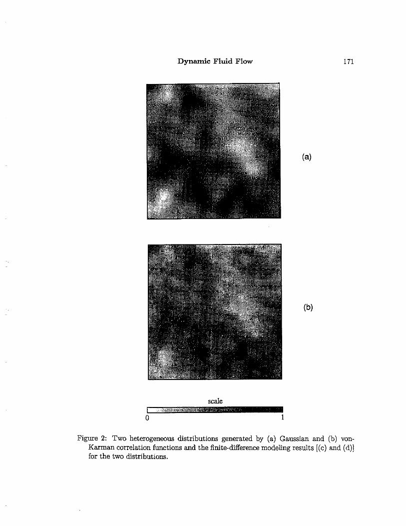
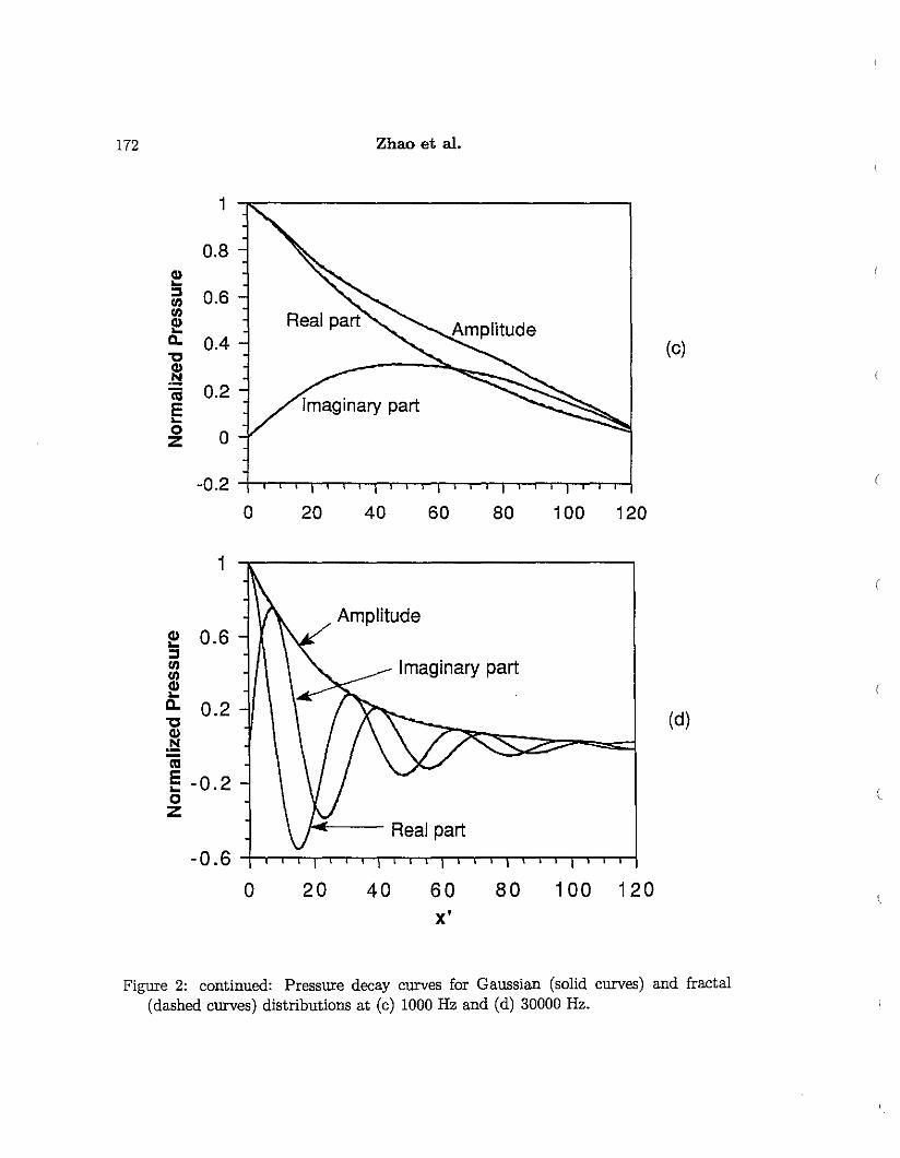
In Figure 2, we show two heterogeneous distributions generated by Gaussian (a) andvon-Karman (b) correlation functions and the finite-difference modeling results for thetwo distributions. The von-Karman dlstribution has a fractal dimension of D = 2.5at small wavelengths (Frankel and Clayton, 1986), and thus it is much rougher thanthe Gaussian distribution. In spite of the roughness, the fluid pressures for the twodistributions are almost the same (Figure 2c and d for frequency = 1000 and 30000Hz, respectively), showing that the dynamic flow is not sensitive to the roughness ofthe heterogeneities as long as the wavelength is greater than the small scale roughness.This is also true for the steady-state flow (Zhao and Toksoz, 1991) and transient flow(Zhao and Toksoz, this volume) cases.

To study the behavior of the heterogeneous porous medlum in conducting the dy­namic flow, we compute the flow rate q", into the medium at the x = 0 boundary,as

q", = ~ {Lv {k(X,y) ap}1 dy.LyJo M ax ",=0

In the logging situation, this flow corresponds to the dynamic flow into a formation dueto the pressure disturbance of the borehole waves. In the effective medium approach,a heterogeneous medium having random variations is often treated as an equlvalenthomogeneous medium whose property (Le., permeability in the present study) is theaverage property of the heterogeneous medium. We have calculated the flow rate forthe heterogeneous medium (generated by Gaussian correlation function) and the homo­geneous medium as a function of frequency using the same parameters as those usedin Figure 1. In Figure 3, we plot the ratio qhete/qhomo versus frequency for differentcorrelation lengths (a = 3, 5, and 10, the model length is 64). Here q is the amplitudeof the complex flow rate of Eq. (19). If the behavior of the heterogeneous medium is thesame as that of the equivalent homogeneous medium, the ratio qhete/qhomo would plotas a horizontal line of height 1. However, this ratio demonstrates a strong frequency­dependent behavior. At very low frequencies, qhete/qhomo is always less than 1. As

164 Zhao et aI.

frequency increases, this ratio increases to reach a maximum. At very high frequen­cies, this ratio approachs a constant. The maximum lies within the transition regionbetween the quasi-static and dynamic regimes and reflects the complexity of dynamicflow in heterogeneous media. The variation of qhete/q/wmo is also a function of the scaleof the heterogeneities. This scale is governed by the correlation length a of the medium.As a increases the range of variation also increases. For example, the curve in Figure 3for the a = 10 case varies by more than 30% from zero frequency to the maximum, whilefor a = 3, this range is reduced about 10%. It can be concluded that when the cor­relation length is very small, the heterogeneous medium will behave like an equivalenthomogeneous medium.

Th above results may have important implications to Stoneley wave logging in aheterogeneous formation. For an average permeability of 1 Darcy, the maximum of theflow ratio is around 5 kHz, within the frequency of Stoneley wave measurements. Inaddition, the borehole diameter is generally on the order of 0.2 m and is in many casescomparable to the scale of formation heterogeneities. When the qhete/qhomo maximumlies within the frequency range of the measurements, more flow will be conducted intoa heterogeneous formation than into a homogeneous formation. It is therefore expectedthat the flow into the heterogeneous formation may signiflcantly affect the Stoneleywave propagation in this formation.

DYNAMIC FLUID FLOW THROUGH A SINGLE FRACTUREWITH ROUGH SURFACES

We now apply the flnite-difference formulation for heterogeneous media to study thedynamic flow in a single fracture with rough surfaces. The roughness of a natural rock

( )-<7-2D)

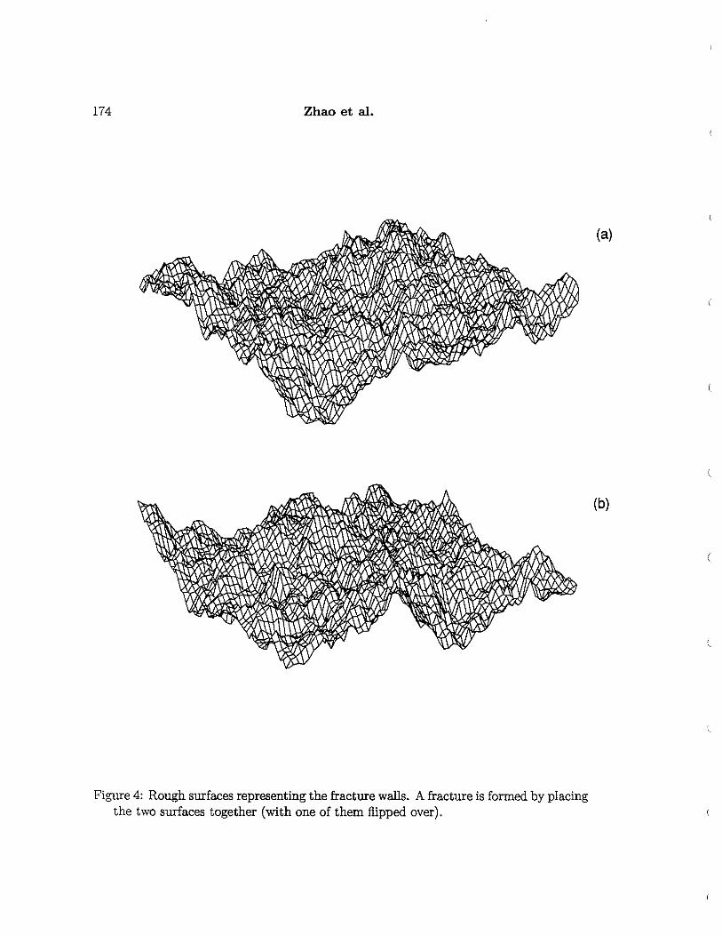
surface has power spectra of the form G(A) ~ :\ (Brown, 1987), where Ais the wavelength, and D is the fractal dimension of the surface and falls in the range2.0 :s D :s 2.5. For this study, the fractal model is assumed to adequately describethe character of rock fractal surfaces. To form a fracture, two surfaces with the samefractal dimension of D = 2.5, but generated with different sets of random numbers, wereplaced together (with one of them flipped over) at some fixed distance dm between themean planes of the two surfaces. Figure 4 shows the two surfaces. The local distancebetween the two surfaces gives the aperture distribution d(x, y). The model surfaces aregenerated using Gaussian random distribution with a standard deviation (T and a von­Karman correlation function having a fractal dimension D = 2.5. When dm = 4.24(T,the two surfaces begin to contact each other. At the "contact", the local apertured(x, y) is set to zero assuming that the deformation of the contact is ignored (Brown,1987). Figure 5 shows examples of the local aperture distribution generated with thetwo surfaces of Figure 4 at various dm values [(a) dm = 1O(T, (b) dm = 3(T, (c) dm = 1(T].For a rough-walled fracture, a measure of aperture in terms of fluid flow is the mean

(

Dynamic Fluid Flow

aperture defined as (Brown, 1987)

if = L:z:1L

y1oL: 10LY

d(x, y)dxdy

The mean aperture represents the aperture available to flow.

165

(20)

(21)

(22)

(23)

If we assume that d(x, y) varies slowly in the plane of the fracture and that thepermeability for a parallel plane fracture holds locally, we then have

k ( ) d2(x,y)

o x,y = 12 .

Eq. (21) gives the static (zero-frequency) permeability distribution over the fractureplane. Applying the dynamic permeability locally, we have

k(w'x y) = d2(x,y)/12

" (1 - iWPod2(x, y)/36/1-)l/2 - iwpod2(x, y)/12/1-

where we have used T = 1 [straight flow at (x, y)] and ¢ = 1 (aperture filled with fluid)in Eq. (5). Tang et al. (1991) showed that Eq. (22) agrees almost exactly with thetheory of dynamic conductivity derived for a parallel wall fracture. With the dynamicpermeability distribution specified for each (x, y) using Eq. (22), the finite-differencetechnique of the previous section is applied to calculate the dynamic fluid flow over the2-D grids for various frequencies and separations dm/a. The results are presented inthe following section.

Numerical Results and Comparison with the Parallel Plate Model

For dynamic fluid flow through a rough-walled fracture, the measurable quantity is theaverage flow rate per unit fracture length into the fracture opening:

- 1 10LY {d( )k(w,X,y)OP}1 dq= - x,y y ,L y 0 /1- ox :z:=o

where k(w,x, y)I:z:=o is the fracture dynamic permeability of Eq. (22) evaluated at x = O.In the borehole situation, the average flow rate ij represents the dynamic flow into aborehole fracture due to the acoustic wave excitation in the borehole.

For the finite-difference modeling, we set L:z: = L y = L = 0.2m, the standarddeviation a "" 1.6/1-m. The flow field through the fracture is computed at increasingfrequency with dm / a equal to various values. The dynamic effects of the fluid motion

are controlled by the thickness of viscous skin depth 8 = ff!i compared to the fracture

aperture if (Johnson et al., 1987; Tang and Cheng, 1989). For water (/1- = 1.14 x 10-3

166 Zhao et al.

Pa s), (j is 19.05 /-Lm at 1000 Hz and 3.48 /-Lm at 30000 Hz. The two surfaces will beginto contact at about 4.26<7 = 6.8 /-Lm. By varying rim/ <7 and frequency, fluid flow ina rough-walled fracture can be simulated for quasi-static as well as dynamic regimes.For each simulated pressure fleld, the pressure gradient at x = 0 is calculated and usedin Eq. (23) to compute the flow rate. For comparison with the parallel plate model,we compute the dynamic flow rate into a plane fracture using the dynamic fractureconductivity c(w, d) (Tang and Cheng, 1989)

if= c(w, d) \7 P (24)

(25)

Assuming a 1-D flow field along a fracture of length L, the pressure in the fractureis given in Eq. (18). We then have

8P cos),L-8 Ix=o = Po(w», . AL .x SIn

In addition, the dynamic conductivity in Eq. (24) is calculated using Eq. (12) of Tangand Cheng (1989) with d of Eq. (20) as the aperture of the equivalent plane fracture.

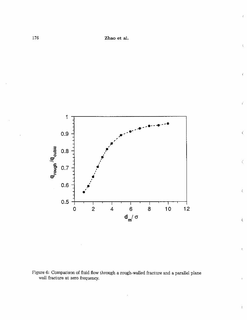
Before we compare the results versus frequency, we show the zero-frequency re­sults calculated using the iterative finite-difference algorithm. The results are shown asqraugh/qplane vs. rim/<7 in Figure 6, where qraugh is the calculated rough-wall flow rateand qplane is the cubic law flow rate calculated using Eqs. (24) and (25) with w = 0,and with the plane fracture thickness equal to dof the rough-walled fracture. The ratioof the mean plane separation dm over standard deviation of the roughness is the stan­dardized separation between the mean planes of the two fracture surfaces. As shownin Figure 6, for small separations, qraugh is significantly reduced compared with qplane

because of the contacting of the rough surfaces. As rim/<7 increases to 10, qraugh/qplane

approaches 1. The overall behavior of qraugh/qplane agrees with the results calculatedby Brown (1987) for the steady flow case.

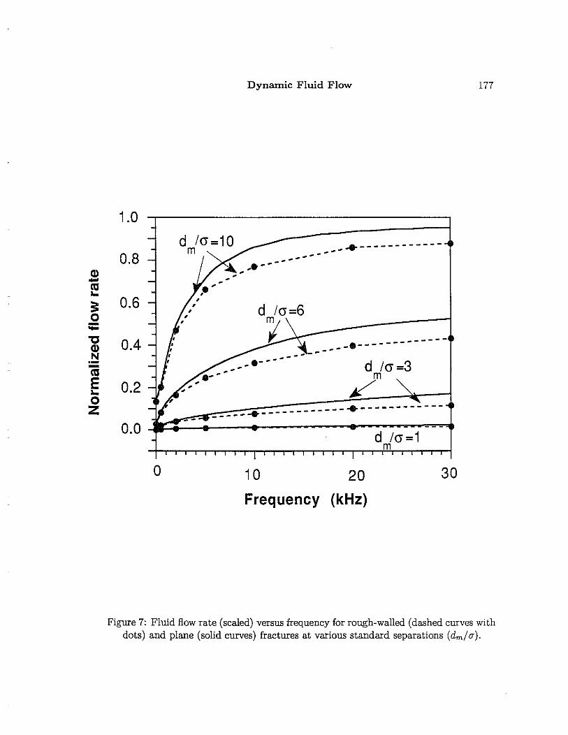
Next, we compare the results for dm /<7 = 1, 3, 6, and 10 and for frequencies rangingfrom 0 to 30000 Hz. Figure 7 shows the calculated rough-walled fracture flow rate qraugh

(solid dots) and the parallel plane fracture flow rate qplane (dashed curves) calculatedusing Eq. (18) with the plane fracture aperture equal to d. As seen from Figure 7,the flow rate shows strong frequency dependence (or dynamic effects), increasing withincreasing frequenCies. Even for the very small fracture with contacting surfaces (e.g.,rim/ <7 = 1 case), the dynamic effect is still significant. The rough-wall fracture flowrate is smaller than that of the equivalent plane fracture. This difference demonstratesthat the effect of the fracture surface roughness is to reduce the fluid flow in static aswell as dynamic regimes. In the high-frequency dynamic regime, the ratio qraugh/qplane

increases to approach 1 as the fracture aperture increases. For example, at 30000 Hz,the ratio for rim/<7 = 1, 3, 6, and 10 are 0.66, 0.68, 0.82, and 0.92, respectively. The high­frequency results are analogous to the results of electrical current through a fracture

Dynamic Fluid Flow 167

modeled by Brown (1989), because in both cases the local fracture conductivities ofboth the high-frequency fluid flow and electrical current are linearly proportional to thelocal aperture (see Brown, 1989 and Tang and Cheng, 1989).

CONCLUSIONS

In this study, we have developed a finite-difference algorithm for simuiating dynamicfluid flow in the frequency domain for an arbitrarily heterogeneous porous media. Aheterogeneous medium behaves differently than a homogeneous medium, especially atlow to medium frequencies. At medium frequencies, the heterogeneous medium conductmore flow than the homogeneous one, depending on the scale of the heterogeneities.In the logging situation, since the formation may contain various heterogeneities, theheterogeneous flow behavior can cause the discrepancy between the fleld observationand the theoretical prediction from Biot's theory for a homogeneous medium.

Applying the finite-difference technique to study the dynamic fluid flow through asingle fracture with rough surfaces, we have demonstrated the effects of surface rough­ness on the dynamic flow. For dynamic as well as steady flow cases, the surface roughnessreduces the amount of fluid flow through the fracture in the static and dynamic regimes.When the separation between the two fracture surfaces is about 10 times the standarddeviation of the roughness, the behavior of the fracture approaches that of a parallelplane fracture

The flnite-difference technique developed here can find usefui applications to thestudy of tube wave propagation in a heterogeneous porous formation. For example,by "developing the frequency-dependent finite-difference algorithm in cylindrical coordi­nates, we can study the propagation of borehole Stoneley waves in relation to the dy­namic fluid flow into a heterogeneous porous formation. We can also model the Stoneleywave reflection and transmission across a natural fracture zone having a heterogeneouspermeability distribution.

ACKNOWLEDGEMENT

We thank Prof. L.W. Gelhar for his helpfui discussion on the finite-difference algorithm.This research was supported by the Borehole Acoustics and Logging Consortium atM.LT., and Department of Energy grant #DE-FG02-86ERI3636.

168 Zhao et al.

REFERENCES

Bernabe, Y., 1991, On the measurement of permeability in anisotropic rocks, in FaultMechanism and Transport Properties of Rocks: A Festchrift in Honor of W.F. Braceedited by B.J. Evans and T.F. Wong, in press, Academic Press, London.

Biot, M.A., 1956a, Theory of propagation of elastic waves in a fluid-saturated poroussolid, I: Low frequency range, J. Acoust. Soc. Am., 28, 168-178.

Biot, M.A., 1956b, Theory of propagation of elastic waves in a fluid-saturated poroussolid, II: Higher frequency range, J. Acoust. Soc. Am., 28, 179-19l.

Brace, W.F., J.B. Walsh, and W.T. Frangos, 1968, Permeability of granite under highpressure, J. Geophys. Res., 73, 2225-2236.

Brown, S.R, 1987., Flow through rock joints: the effect of surface roughness, J. Geophys.Res., 92, 1337-1347

Brown, S.R., 1989, Transport of fluid and electric current through a single fracture, J.Geophys. Res., 94, 9429-9438.

Brown, S.R., and C.H. Scholz, 1985a, The closure of random elastic surfaces in contact,J. Geophys. Res., 90,5531-5545.

Brown S.R, and C.H. Scholz, 1985b, Broad bandwidth study of the topography ofnatural rock surfaces, J. Geophys. Res., 90, 12575-12582.

Ferziger, J.H., 1981, Numerical Methods for Engineering Applications, John Wiley &Sons, Inc., New York.

Frankel, A., and R Clayton, 1986, Finite difference simulations of seismic scattering: im­plications for the propagation of short-period seismic waves in the crust and modelsof crustal heterogeneity, J. Geophys. Res., 91, 6465-6489.

Hornby, B.E., D.L. Johnson, K.H. Winkler, and RA. Plumb, 1989, Fracture evaluationusing reflected Stoneley-wave arrivals, Geophysics, 54, 1274-1288.

Johnson, D.L., J. Koplik, and R Dashen, 1987, Theory of dynamic permeability andtortuosity in fluid-saturated porous media, J. Fluid Mech., 176, 379-400.

Kamath, J, RE. Boyer, and F.M. Nakagawa, 1990, Characterization of core scale het­erogeneities using laboratory pressure transients, Society of Petroleum Engineers,475-488.

Melville, J.G., F.J. Molz, O. Gaven, and M.A. Widdowson, 1991, Multilevel slug testswith comparisons to tracer data, Ground Water, 29, 897-907.

(

Dynamic Fluid Flow 169

Paillet, F.L., C.H. Cheng, and X.M. Tang, 1989, Theoretical models relating acoustictube-wave attenuation to fracture permeability - reconciling model results with fielddata, Trans., Soc. Prof. Well Log Analyst, 30th Ann. Symp.

Tang, X.M., and C.H. Cheng, 1989, A dynamic model for f1uld flow in open boreholefractures, J. Geophys. Res., 94, 7567-7576.

Tang, X.M., C.Ho Cheng, and MoNo Toksoz, 1991, Dynamic permeability and boreholeStoneley waves: A simplified Biot-Rosenbaum model, J. Acoust. Soc. Am., 90, 1632­1646.

Zhao, X.Mo, and M.No Toksoz, 1991, Permeability anisotropy in heterogeneous porousmedia, 61st SEG Ann. Mtgo Expanded Abstracts, 387-390

Zhao, X.M., and M.N. Toksoz, Transient fluid flow in heterogeneous porous media, thisvolume.

Zimmerman, R.W., S. Kumar, and G.S. Bodvarsson, 1991, Lubrication theory analysis ofthe permeability of rough-walled fractures, Int. J. Rock. Mech. Min. Sci. fj Geomech.Abstr., 28, 325-331.

170 Zhao et al.

0.8 Amplitudel!!:::J 0.6'"'"l!!

(a)a. 0.4 Real part."..•!:O!0; 0.2§0

0z Imaginary part

-0.2

0 20 40 60 80 100 120

0.8 Amplitude

l!! (:::J 0.6'"'"l!! Real parta. 0.4 (b)."

.~0.2

Imaginary part0;E-0 0 •z ,

-0.20 20 40 60 80 100 120

Amplitude

o

l!!:::J 0.5'"£."

.~0;§oZ

Real part

(c)

(

o 20 40 60 80 100 120x·

Figure 1: Comparison of finite-difference pressure decay curves along model length x'(dashed curves with dots) with 1-D analytic results (solid curves) for a homogeneousdistribution at various frequencies. The frequencies are (a) 100 Hz, (b) 5000 Hz, and(c) 2'0000 Hz.

Dynamic Fluid Flow

scale

o

(a)

(b)

171

Figure 2: Two heterogeneous distributions generated by (a) Gaussian and (b) von­Karman correlation functions and the finite-difference modeling results [(c) and (d)]for the two distributions.

172 Zhao et al.

Figure 2: continued: Pressure decay curves for Gaussian (solid curves) and fractal(dashed curves) distributions at (c) 1000 Hz and (d) 30000 Hz.

Dynamic Fluid Flow

1.2 ,--------------...,

173

cerr. length =5

til:::l0Gll:: 1.1Qltll0E0.c:

~ 1til:::l0Qll::Gltll 0.90..Gl....Gl.c:

C"

0.8

cerr. length =10

/........ - ...............~€l -~-- ..-----

------e------e-----­~~------.------.------

\cerr. length = 3

o 5 10 15

Frequency

20

(kHz)

25 30

Figure 3: Fluid flow ratios through a heterogeneous and a homogeneous medium asfunctions of frequency.

174 Zhao et al.

(a)

(b)

(

Figure 4: Rough surfaces representing the fracture walls. A fracture is formed by placingthe two surfaces together (with one of them flipped over).

DynlUIlic Fluid Flow 175

(a)

(b)

(e)

Figure 5: Examples of local aperture distribution formed using the two rough surfacesin Figure 4 with dm/cy = 10 (a), 3 (b), and 1 (e).

176 Zhao et al.

1.... --..--

. .... --_.- - (0.9 ~ ,.-,,II

() ,:c 0.8 - ,.::s ,() ,

•C- ,(-- ,

.c •Cl 0.7 - •::s •0 •.. •

C- ••,0.6 - •,.

,•

0.5 , I I I I T

0 2 4 6 8 10 12d /am

Figure 6: Comparison of fluid flow through a rough-walled fracture and a parallel planewall fracture at zero frequency.

Dynamic Fluid Flow 177

0.8

1.0

Q)-coI-

;: 0.6o;;::

-_ ... -------------------.... ---

0.4 -----­e------­------d /(J =3

m

0.21~~_~__:__~.~-=-_:__~__~__~__:_..:~=_~__:__=__~__~__]--0.0 d /(J =1

m

"CQ)N.-a;EI-oZ

o 10 20

Frequency (kHz)

30

Figure 7: Fluid flow rate (scaled) versus frequency for rough-walled (dashed curves withdots) and plane (solid curves) fractures at various standard separations (dm / o)

178 Zhao et al.

(

(