－119－

Dynamic Effects of Changes in Interest Rates and Exchange Rates on the Stock Market Return in Bangladesh

Prashanta K. BanerjeeBishnu Kumar Adhikary

Summary

Investigation of the exchange rate reveals a short term net negative feedback from the exchange rate to stock market with insignificant associated T-values of the coefficients of the contemporaneous and lagged variables. It shows that the exchange rate and stock market are nearly independent, which is also evidenced by the R2 and F statistics. This is because foreign portfolio investment is very limited in Bangladeshi stock markets, particularly after 1996, which results in little impact of changes in foreign exchange rates on stock market returns in Bangladesh.

Introduction

A number of macroeconomic and financial variables that influence the stock market have been documented in recent empirical studies, without a consensus on their appropriateness as regressors (Lanne 2002, Campbell and Yogo 2003, Jansen and Moreira 2004, Donaldson and Maddaloni 2002, Goyal 2004, and Ang and Maddaloni 2005). Frequently cited variables are GDP, price level, industrial production rate, interest rate, exchange rate, current account balance, unemployment rate, fiscal balance, etc. A very few studies have been carried out examining the direct effects of the above variables on stock market return in Bangladesh. This paper investigates empirically the dynamic effects of changes in interest rates and exchange rates on the overall stock market return in Bangladesh.

The rationale for a relationship between interest rates and stock market return is that stock prices and interest rates are negatively correlated. A higher interest rate ensuing from contractionary monetary policy usually affects stock market return negatively. This is because higher interest rates reduce the value of equity as stipulated by the dividend discount model; make fixed income securities more attractive as an alternative to holding stocks; may reduce the propensity of investors to borrow and invest in stocks; and raise the cost of doing business, hence affecting profit margins. On the other hand, lower interest rates resulting from expansionary monetary policy tend to boost the stock market.

There are interactions between national stock markets and exchange rates through changes in foreign investment. Rates of return on foreign investment in stocks are converted from one currency into another currency through changing spot exchange rates. When rates of return in a depreciating currency are translated into a stronger currency, the adjusted rates of return decline. In contrast, when rates of return in an appreciating currency are translated into a depreciating currency, the adjusted rates of return increase. Foreign portfolio investors pay close attention to timing their return conversions based on the anticipated exchange rate movements. Moreover, increasing foreign investments in a country’s stock market cause the local currency to appreciate vis-à-vis a related foreign

－120－

currency through larger foreign currency inflows. Conversely, sales of a country’s stocks by foreign investors cause foreign capital outflows, which in turn make the local currency depreciate against a related foreign currency. The depictions of such relationships between stock and foreign currency markets have possible flows of bidirectional causality. As currency depreciation and uncertainty adversely affect stock market returns, international fund managers readjust their stock market investment decisions.

This study examines whether stock market return is influenced by changes in interest rates and exchange rates in Bangladesh. This country has been selected because of its growing importance in the Asian economy due to increasing market openness, a continuing and unfolding strong trade relationship with the outside world, rising foreign investment, an expanding GDP growth rate, and enduring expansion in export-oriented industry and services. Trade openness reached 34.23 per cent in 2005 from 2.03 per cent in 1976. GDP expanded by 5.9 per cent in 2005, up from 4.6 per cent in 1979. Foreign investment grew 152.67 per cent during the period 1996-2006. Exports and imports grew 143.43 percent and 135.21 percent respectively during the period 2000-2006. A floating exchange rate system has been used since May, 2003.

The financial sector of Bangladesh is overwhelmingly bank based, with 49 banks accounting for about 95 per cent of the sector’s resources (Asian Development Outlook 2005). Both institutional and individual investors invest their savings mainly in banks and financial institutions on fixed term deposits. In addition, individual investors contemplate long term government securities as one of their prioritized investment instruments. High interest rates offered by banks and financial institutions on fixed deposits and by government in long-term government saving instruments have discouraged the development of a share market. Government has taken action for the reduction and rationalization of interest rates. Interest rates continued to decline in FY2005, aided by a reduction in the statutory liquidity requirement, lower rates offered on government national savings certificates, and improved supervision and corporate governance in commercial banks (ADB outlook 2005). Even after this, interest rates on fixed term deposits and long-term government securities seem rewarding to investors.

The remainder of the paper proceeds as follows. Section 2 provides a brief survey of the relevant literature. Section 3 describes the data and outlines the empirical design. Section 4 reports the empirical results, and Section V offers concluding remarks.

Brief Literature Survey

The evolving empirical literature on linkages between stock markets and foreign exchange markets relates to both developed and developing countries, although their financial markets are not equally developed. However, both developed and developing countries can benefit from each other by sharing their pertinent experiences, as the foreign currency and stock markets are subject to uncertainties. The classic theories have sought a statistically significant relationship between exchange rates and equity returns. Frank and Young (1972), who are considered pioneers in examining the relationship between the exchange rate and the stocks of US multinational firms, concluded that there exists no definite or uniform pattern of stock price reaction to exchange rate realignment. On the other hand, Ang and Ghallab (1976) studied the effect of US Dollar devaluation on 15 US multinational firms’ stocks for the period from August 1971 to March 1973, and reported that the stock market was efficient and that stock prices adjusted rapidly to the exchange

－121－

rate. Similarly, Aggarwal (1981) discovered that the floating value of the US Dollar and US stock prices were positively correlated for the period from 1974-1978. In 1987, Levy (1987) examined the impact of the changes in the US Dollar on the real values of before-tax corporate profits on a sectoral basis. He indicated that the US Dollar exchange rate could adversely affect firms’ before-tax profits in general, but that the degree of impact varied sectorally. He also concluded that US Dollar changes had the largest impact on profits of durable goods manufacturers as compared to certain service industries. Conversely, a very weak relation between the changes in the US Dollar exchange rate and the stock market (industrial stock prices indices) was reported by Sonnen and Hennigar in 1998, which they referred to as a negative relation. Bahmani-Oskooee and Sorabian (1993) concluded that there exists a bi-directional causality between stock prices and exchange rate, at least in the short run, although their co-integration analysis does not show any long-term relationship between these variables. However, a study conducted by Qiao (1997) reported that a bi-directional relationship existed in the stock prices and exchange rate of the Tokyo stock market.

In Australia, Loudun (1993) studied stock return sensitivity for a sample of Australian companies with respect to change in the trade weighted index value of the Australian Dollar during the post-float period from January 1984 to December 1989. He found that resource stocks and industrial stocks respond differently to fluctuations in the value of the Australian dollar. In 2000, Ariffin and Hook investigated the relationship between the exchange rate of the Malaysian Ringgit in terms of US Dollars and stock prices in Kuala Lumpur Stock Exchange (KLSE) using single index and multi index models. They documented a negative relation between exchange rates and stock prices in the KLSE market.

Regarding the relationship between stock prices and interest rates, a number of empirical studies have been undertaken since the 1970s. Fama (1981, 1990), Chen, Roll and Ross (1986) and Chen (1991) tested the relationships between macroeconomic variables and stock prices with US economic data. Fama (1981) documented a strong positive correlation between common stock returns and real economic variables like capital expenditure, industrial production, real GNP, money supply, lagged inflation and interest rates. Chen, Roll and Ross (1986) found that the changes in aggregate production, inflation, the short-term interest rates, the maturity risk premium and default risk premium are the economic factors that explain changes in stock prices. Smirlock and Yawitz (1985) stated that interest rate changes can impact equity prices through two conduits: by affecting the rate at which the firm’s expected future cash flows will be capitalized, and by altering expectations about future cash flows. In particular, they argued that an increase in interest rates causes stock prices to decline and a decline in interest rates causes stock prices to rise. Further, they argued that if both capitalization rates and expectations about future cash flows are impacted by interest rates, these effects would influence equity prices.

Hardouvelis (1987) pointed out that there exists an inverse relationship between stock prices and changes of interest rates, and that this can be rationalized in terms of money supply surprises. The negative (positive) reaction of stock prices (interest rates) to money supply surprises can be explained in terms of the following two hypotheses. The expected real interest rate hypothesis claims that stock prices decline because the real component of nominal interest rates is expected to increase, thereby increasing the discount rate at which future cash flows are capitalized and also because higher interest rates affect real output adversely, thereby reducing future operating cash flows. The expected

－122－

inflation hypothesis claims that stock prices decline because the inflation premium in nominal interest rates increases, which decreases the after-tax real dividends. In Japan, Elton and Gruber (1988) applied arbitrage pricing theory (APT) to Japanese stock returns and several macroeconomic variables like industrial production, money supply, crude oil price, and short-term interest rates, and showed that there existed a positive relationship between stock prices and short-term interest rates.

Thorbecke and Alami (1994) and Jensen et al. (1997) have shown that changes in federal funds rate influence equity prices. Thorbecke (1997) studied the effects of actual changes in the fed funds rate, targeting the Dow Jones Industrial and Composite averages over the 24 hours following the news of the target change. He found that fed funds rate changes are inversely related to stock prices and that monetary policy has a large effect on ex ante and ex post stock returns. Chen et al. (1999) examined the effect of discount rate changes on the volatility of stock prices and on trading volume. They discovered that unexpected discount rate changes contributed to higher, though short-lived, volatility and trading volume. Ying Wu (2001) examined the impact of macroeconomic variables on the Straits Times Industrial Index (STII) by categorizing the macroeconomic indicators into two groups: money supply and interest rates. He documented how the money supply does not register any pattern of influence on the STII, though the interest rate does play a significant role in determining the STII on the monthly investment horizon. Wing et al. (2005) examined the long-run equilibrium relationships between the major stock indices of Singapore and the United States using selected macroeconomic variables, applying time series data for the period January 1982 to December 2002. The results of their cointegration test suggest that Singapore’s stock prices generally display a long-run equilibrium relationship with interest rates and money supply (M1), but that a similar relationship does not exist in the United States.

Data Description and Empirical Design

(a) Data description

The monthly data employed in this paper range from January, 1983 through December, 2006. The use of monthly data avoids the problems of thin trading and price limits in a stock market (Shen and Wang, 1997). As stock market data, the DSE (Dhaka Stock Exchange) all share price indices were collected from issues of “Economic Trends” – a monthly economic report published by the statistics department of Bangladesh Bank. The weighted average interest rates on bank deposits have been used for the interest rate in this research, since savers of Bangladesh commonly invest their savings in bank deposits for a certain higher interest rate when investment in the share market does not seem profitable to them. The exchange rate between the Bangladeshi Taka and the U.S. Dollar has been used for the exchange rate, in view of the dominance of the U.S. Dollar in international transactions and trade, as well as financial relationship of the Bangladesh economy with the U.S. economy. Both the interest rate and exchange rate data have been collected from monthly issues of International Financial Statistics published by the International Monetary Fund (IMF).

－123－

(b) Empirical Design

The base estimating equation in log-linear form is as follows:

lnYt = � + � lnIR t+ � lnEXt +et (1)

Where, Y = stock market return of Bangladesh, IR = interest rate and EX = exchange rate. There are two reasons why variables are converted into natural logs. First, the coefficients of the cointegrating vector can be interpreted as long-term elasticities if the variables are in logs. Secondly, if the variables are in logs, the first difference can be

interpreted as growth rates. The expected signs are � >0, �<0 and��

� 0. The error-

term (e) is assumed to be independently and identically distributed. The additional symbol (t) is used as the time subscript.

For execution of the empirical design, the nature of the data distribution is examined first using standard descriptive statistics (mean, median, standard deviation, skewness and kurtosis). The normality of data distribution is also ascertained by invoking the Jarque-Bera test.

Second, the time series property of each variable is investigated using univariate analysis by implementing the ADF (Augmented Dickey-Fuller Test) for the unit root (nonstationarity) (following Dickey and Fuller, 1981 and Fuller, 1996). Likewise, the PP (Phillips-Perron) test is also implemented (following Phillips, 1986; Phillips and Perron, 1988; Perron, 1989). The KPSS (Kwiatkowski, Philips, Schmidt and Shin) test for no unit root (stationarity) is applied as a counterpart of ADF and PP tests (following Kwiatkowski, et al., 1992).

Third, if these tests confirm the stationarity in time series data of each variable, equation (1) is estimated appropriately by the Ordinary Least Square (OLS) method. Otherwise, its application leads to misleading inferences in the presence of spurious correlation (Granger and Newbold, 1974).

Fourth, in the event of the nonstationarity of each variable, the cointegrating relationship among variables (the tendency for variables to move together in the long run) is studied either by the Engle-Granger (1987) procedure or the Johansen-Juselius procedure (Johansen 1988; Johansen-Juselius 1992, 1999) to overcome the associated problem of spurious correlation and misleading inferences. For both procedures, all the variables must have the same order of integration or depiction of I(1) behavior. However, the Johansen procedure is applied here to test for cointegration. To do this, a Vector Autoregressive (VAR) approach is followed as outlined in Granger (1988). The appropriate lag-length (p) is selected with the aid of the FPE (Final Prediction Error) criterion (Akaike, 1969) to ensure that errors are white noise. This helps overcome the problem of over/underparameterization that may induce bias and inefficiency in the estimates. The analysis commences with a congruent statistical system of unrestricted reduced forms as follows:

Yt = � + Y it

P

i ����

1 + � t; � t ~ IN (0, �), i=1, 2, 3, ----T _------------------------------------ (2)

－124－

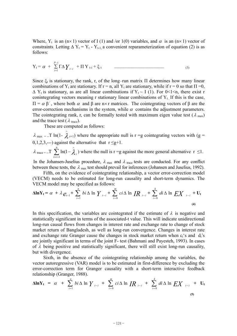
Where, Yt is an (n�1) vector of I (1) and /or 1(0) variables, and � is an (n�1) vector of constraints. Letting � Yt = Yt - Yt-1, a convenient reparameterization of equation (2) is as follows:

Yt = � + Y it

P

i �

�

����

1

1 + � Y t-i + � t ----------------------------------------------- (3)

Since �t is stationary, the rank, r, of the long–run matrix � determines how many linear combinations of Yt are stationary. If r = n, all Yt are stationary, while if r = 0 so that � =0, � Yt is stationary, as are all linear combinations if Yt ~ I (1). For 0<1<n, there exist r conintegrating vectors meaning r stationary linear combinations of Yt . If this is the case, � = � � / , where both � and � are n� r matrices. The cointegrating vectors of � are the error-correction mechanisms in the system, while � contains the adjustment parameters. The cointegrating rank, r, can be formally tested with maximum eigen value test (� max)and the trace test (� trace).

These are computed as follows:

� max = --T ln(1- ��

r+1) where the appropriate null is r =g cointegrating vectors with (g = 0,1,2,3,---) against the alternative that r �g+1.

� trace = --T i

n

ri��

��

�� 1ln(1

) where the null is r =g against the more general alternative r �1.

In the Johansen-Juselius procedure, � max and � trace tests are conducted. For any conflict between these tests, the � max test should prevail for inferences (Johansen and Juselius, 1992).

Fifth, on the evidence of cointegrating relationship, a vector error-correction model (VECM) needs to be estimated for long-run causality and short-term dynamics. The VECM model may be specified as follows:

�lnYt = � + et 1�� + ��

��

n

iitYbi

1ln + �

��

�m

iitIRci

0ln + �

��

�k

iitEXdi

0ln + Ut

(4)

In this specification, the variables are cointegrated if the estimate of � is negative and statistically significant in terms of the associated-t value. This will indicate unidirectional long-run causal flows from changes in interest rate and exchange rate to change of stock market return of Bangladesh, as well as long-run convergence. Changes in interest rate and exchange rate Granger cause the changes in stock market return when ci‘s and di’s are jointly significant in terms of the joint F- test (Bahmani and Payesteh, 1993). In cases of � being positive and statistically significant, there will still exist long-run causality, but with divergence.

Sixth, in the absence of the cointegrating relationship among the variables, the vector autoregressive (VAR) model is to be estimated in first-difference by excluding the error-correction term for Granger causality with a short-term interactive feedback relationship (Granger, 1988).

�lnYt = � + ��

��

n

iitYbi

1ln + �

��

�m

iitIRci

0ln + �

��

�k

iitEXdi

0ln + Ut

(5)

－125－

Impulse response analysis is also performed in this paper by giving a shock of one standard deviation ( ± 2 S.E. innovations) to the interest rate and exchange rate to visualize the duration of their effects on the stock market of Bangladesh. Finally, variance decomposition analysis is also conducted to gain additional insights.

Results

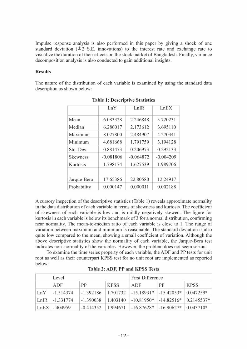
The nature of the distribution of each variable is examined by using the standard data description as shown below:

Table 1: Descriptive StatisticsLnY LnIR LnEX

Mean 6.083328 2.246848 3.720231 Median 6.286017 2.173612 3.695110 Maximum 8.027800 2.484907 4.270341 Minimum 4.681668 1.791759 3.194128 Std. Dev. 0.881473 0.206973 0.292133 Skewness -0.081806 -0.064872 -0.004209 Kurtosis 1.798174 1.627539 1.989706

Jarque-Bera 17.65386 22.80580 12.24917 Probability 0.000147 0.000011 0.002188

A cursory inspection of the descriptive statistics (Table 1) reveals approximate normality in the data distribution of each variable in terms of skewness and kurtosis. The coefficient of skewness of each variable is low and is mildly negatively skewed. The figure for kurtosis in each variable is below its benchmark of 3 for a normal distribution, confirming near normality. The mean-to-median ratio of each variable is close to 1. The range of variation between maximum and minimum is reasonable. The standard deviation is also quite low compared to the mean, showing a small coefficient of variation. Although the above descriptive statistics show the normality of each variable, the Jarque-Bera test indicates non–normality of the variables. However, the problem does not seem serious.

To examine the time series property of each variable, the ADF and PP tests for unit root as well as their counterpart KPSS test for no unit root are implemented as reported below:

Table 2: ADF, PP and KPSS Tests

Level First DifferenceADF PP KPSS ADF PP KPSS

LnY -1.514374 -1.392186 1.701732 -15.18931* -15.42053* 0.047259*LnIR -1.331774 -1.390038 1.403140 -10.81950* -14.82516* 0.2145537*LnEX -.404959 -0.414352 1.994671 -16.87628* -16.90627* 0.043710*

－126－

The Mackinnon (1996) critical values are -3.699871 and -2.976263 at 1 per cent and 5 per cent levels of significance, respectively. The KPSS critical values (Kwiatkowski,et al., 1992, Table 1) are 0.73900 and 0.46300 at 1 per cent and 5 per cent levels of significance, respectively. * indicates stationarity at the first differencing.

The calculated ADF and PP statistics cannot reject the null hypothesis of unit root at either the 1 per cent or 5 per cent significance levels when compared with the respective critical values. The calculated KPSS statistics also clearly reject the null hypothesis of no unit root at both the 1 and 5 per cent levels when compared with the corresponding critical values. In other words, the ADF, PP and KPSS tests decisively confirm the nonstationarity of each variable. Table 2 shows further that LnY, LnIR and LnEX possess I(1) behavior. To be precise, the stationarity of all variables is restored on first differencing, showing the same order of integration.

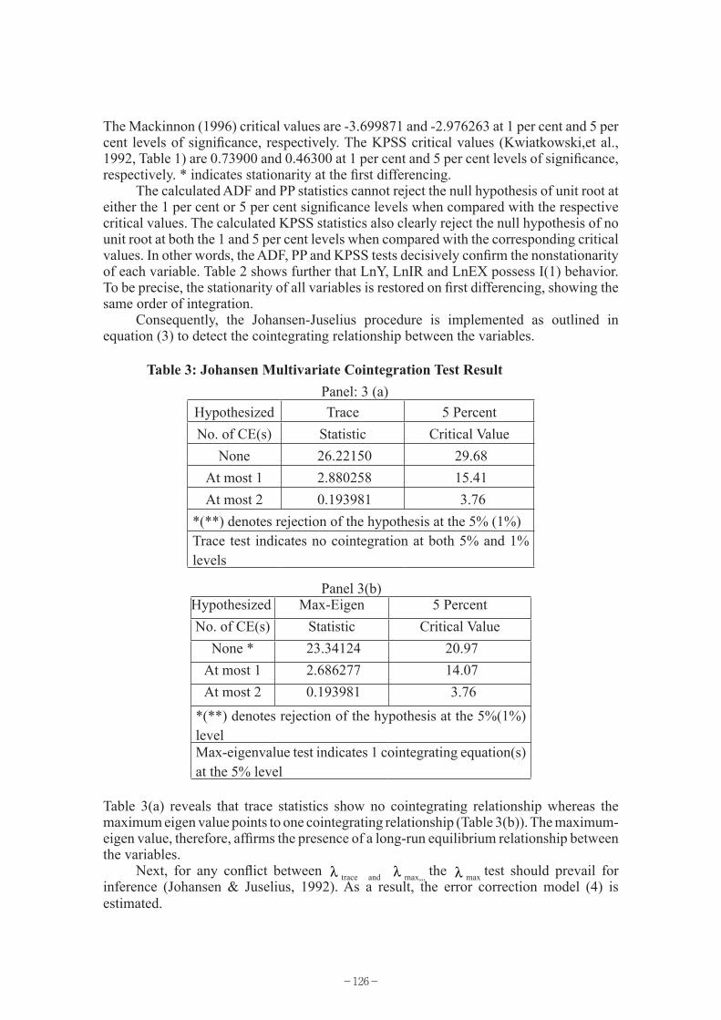
Consequently, the Johansen-Juselius procedure is implemented as outlined in equation (3) to detect the cointegrating relationship between the variables.

Table 3: Johansen Multivariate Cointegration Test Result Panel: 3 (a)

Hypothesized Trace 5 PercentNo. of CE(s) Statistic Critical Value

None 26.22150 29.68At most 1 2.880258 15.41At most 2 0.193981 3.76

*(**) denotes rejection of the hypothesis at the 5% (1%) Trace test indicates no cointegration at both 5% and 1% levels

Panel 3(b)Hypothesized Max-Eigen 5 PercentNo. of CE(s) Statistic Critical Value

None * 23.34124 20.97At most 1 2.686277 14.07At most 2 0.193981 3.76

*(**) denotes rejection of the hypothesis at the 5%(1%) levelMax-eigenvalue test indicates 1 cointegrating equation(s) at the 5% level

Table 3(a) reveals that trace statistics show no cointegrating relationship whereas the maximum eigen value points to one cointegrating relationship (Table 3(b)). The maximum-eigen value, therefore, affirms the presence of a long-run equilibrium relationship between the variables.

Next, for any conflict between λ trace and λ max,,, the λ max test should prevail for inference (Johansen & Juselius, 1992). As a result, the error correction model (4) is estimated.

－127－

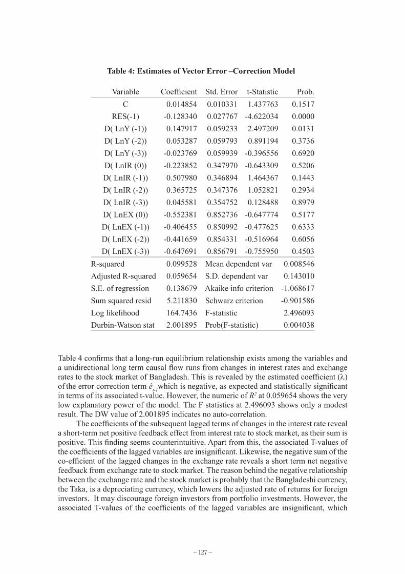
Table 4: Estimates of Vector Error –Correction Model

Variable Coefficient Std. Error t-Statistic Prob. C 0.014854 0.010331 1.437763 0.1517

RES(-1) -0.128340 0.027767 -4.622034 0.0000D( LnY (-1)) 0.147917 0.059233 2.497209 0.0131D( LnY (-2)) 0.053287 0.059793 0.891194 0.3736D( LnY (-3)) -0.023769 0.059939 -0.396556 0.6920D( LnIR (0)) -0.223852 0.347970 -0.643309 0.5206D( LnIR (-1)) 0.507980 0.346894 1.464367 0.1443D( LnIR (-2)) 0.365725 0.347376 1.052821 0.2934D( LnIR (-3)) 0.045581 0.354752 0.128488 0.8979D( LnEX (0)) -0.552381 0.852736 -0.647774 0.5177D( LnEX (-1)) -0.406455 0.850992 -0.477625 0.6333D( LnEX (-2)) -0.441659 0.854331 -0.516964 0.6056D( LnEX (-3)) -0.647691 0.856791 -0.755950 0.4503

R-squared 0.099528 Mean dependent var 0.008546Adjusted R-squared 0.059654 S.D. dependent var 0.143010S.E. of regression 0.138679 Akaike info criterion -1.068617Sum squared resid 5.211830 Schwarz criterion -0.901586Log likelihood 164.7436 F-statistic 2.496093Durbin-Watson stat 2.001895 Prob(F-statistic) 0.004038

Table 4 confirms that a long-run equilibrium relationship exists among the variables and a unidirectional long term causal flow runs from changes in interest rates and exchange rates to the stock market of Bangladesh. This is revealed by the estimated coefficient (λ) of the error correction term êt-1which is negative, as expected and statistically significant in terms of its associated t-value. However, the numeric of R2 at 0.059654 shows the very low explanatory power of the model. The F statistics at 2.496093 shows only a modest result. The DW value of 2.001895 indicates no auto-correlation.

The coefficients of the subsequent lagged terms of changes in the interest rate reveal a short-term net positive feedback effect from interest rate to stock market, as their sum is positive. This finding seems counterintuitive. Apart from this, the associated T-values of the coefficients of the lagged variables are insignificant. Likewise, the negative sum of the co-efficient of the lagged changes in the exchange rate reveals a short term net negative feedback from exchange rate to stock market. The reason behind the negative relationship between the exchange rate and the stock market is probably that the Bangladeshi currency, the Taka, is a depreciating currency, which lowers the adjusted rate of returns for foreign investors. It may discourage foreign investors from portfolio investments. However, the associated T-values of the coefficients of the lagged variables are insignificant, which

－128－

indicates a very subdued influence of the exchange rate on stock market return. The optimum number of lags is determined by the AIC criterion, as stated earlier.

Next, the Monte Carlo Experiments reported in Cheung and Lai (1993) suggest that the trace test shows more robustness to both skewness and excess kurtosis in the residuals than the maximum eigen value. Table 3 (a) shows that, as per the trace statistics, no cointegration prevails in the system. As a result, the null hypothesis of no cointegration cannot be rejected. In this regard, VAR is estimated by following equation (5).

Table 5: Vector Autoregressive Model

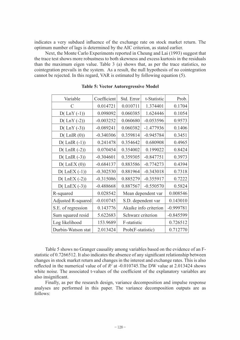
Variable Coefficient Std. Error t-Statistic Prob. C 0.014721 0.010711 1.374401 0.1704

D( LnY (-1)) 0.098092 0.060385 1.624446 0.1054D( LnY (-2)) -0.003252 0.060680 -0.053596 0.9573D( LnY (-3)) -0.089241 0.060382 -1.477936 0.1406D( LnIR (0)) -0.340306 0.359814 -0.945784 0.3451D( LnIR (-1)) 0.241478 0.354642 0.680908 0.4965D( LnIR (-2)) 0.070454 0.354002 0.199022 0.8424D( LnIR (-3)) -0.304601 0.359305 -0.847751 0.3973D( LnEX (0)) -0.684137 0.883586 -0.774273 0.4394D( LnEX (-1)) -0.302530 0.881964 -0.343018 0.7318D( LnEX (-2)) -0.315086 0.885279 -0.355917 0.7222D( LnEX (-3)) -0.488668 0.887567 -0.550570 0.5824

R-squared 0.028542 Mean dependent var 0.008546Adjusted R-squared -0.010745 S.D. dependent var 0.143010S.E. of regression 0.143776 Akaike info criterion -0.999781Sum squared resid 5.622683 Schwarz criterion -0.845599Log likelihood 153.9689 F-statistic 0.726512Durbin-Watson stat 2.013424 Prob(F-statistic) 0.712770

Table 5 shows no Granger causality among variables based on the evidence of an F-statistic of 0.7266512. It also indicates the absence of any significant relationship between changes in stock market return and changes in the interest and exchange rates. This is also reflected in the numerical value of of R2 at -0.010745.The DW value at 2.013424 shows white noise. The associated t-values of the coefficient of the explanatory variables are also insignificant.

Finally, as per the research design, variance decomposition and impulse response analyses are performed in this paper. The variance decomposition outputs are as follows:

－129－

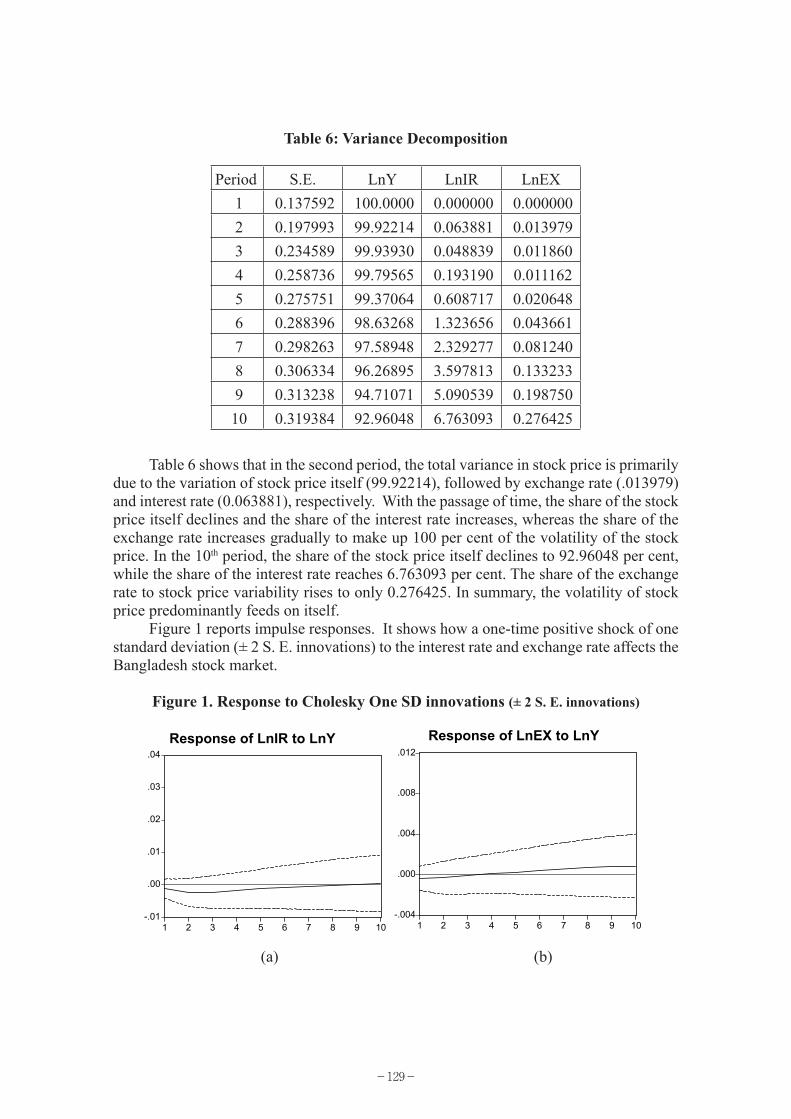
Table 6: Variance Decomposition

Period S.E. LnY LnIR LnEX 1 0.137592 100.0000 0.000000 0.000000 2 0.197993 99.92214 0.063881 0.013979 3 0.234589 99.93930 0.048839 0.011860 4 0.258736 99.79565 0.193190 0.011162 5 0.275751 99.37064 0.608717 0.020648 6 0.288396 98.63268 1.323656 0.043661 7 0.298263 97.58948 2.329277 0.081240 8 0.306334 96.26895 3.597813 0.133233 9 0.313238 94.71071 5.090539 0.198750 10 0.319384 92.96048 6.763093 0.276425

Table 6 shows that in the second period, the total variance in stock price is primarily due to the variation of stock price itself (99.92214), followed by exchange rate (.013979) and interest rate (0.063881), respectively. With the passage of time, the share of the stock price itself declines and the share of the interest rate increases, whereas the share of the exchange rate increases gradually to make up 100 per cent of the volatility of the stock price. In the 10th period, the share of the stock price itself declines to 92.96048 per cent, while the share of the interest rate reaches 6.763093 per cent. The share of the exchange rate to stock price variability rises to only 0.276425. In summary, the volatility of stock price predominantly feeds on itself.

Figure 1 reports impulse responses. It shows how a one-time positive shock of one standard deviation (± 2 S. E. innovations) to the interest rate and exchange rate affects the Bangladesh stock market.

Figure 1. Response to Cholesky One SD innovations (± 2 S. E. innovations)

12

Table 6: Variance Decomposition

Period S.E. LnY LnIR LnEX 1 0.137592 100.0000 0.000000 0.000000 2 0.197993 99.92214 0.063881 0.013979 3 0.234589 99.93930 0.048839 0.011860 4 0.258736 99.79565 0.193190 0.011162 5 0.275751 99.37064 0.608717 0.020648 6 0.288396 98.63268 1.323656 0.043661 7 0.298263 97.58948 2.329277 0.081240 8 0.306334 96.26895 3.597813 0.133233 9 0.313238 94.71071 5.090539 0.198750 10 0.319384 92.96048 6.763093 0.276425

Table 6 shows that in the second period, the total variance in stock price is primarily due to the variation of stock price itself (99.92214), followed by exchange rate (.013979) and interest rate (0.063881), respectively. With the passage of time, the share of the stock price itself declines and the share of the interest rate increases, whereas the share of the exchange rate increases gradually to make up 100 per cent of the volatility of the stock price. In the 10th period, the share of the stock price itself declines to 92.96048 per cent, while the share of the interest rate reaches 6.763093 per cent. The share of the exchange rate to stock price variability rises to only 0.276425. In summary, the volatility of stock price predominantly feeds on itself.

Figure 1 reports impulse responses. It shows how a one-time positive shock of one standard deviation (± 2 S. E. innovations) to the interest rate and exchange rate affects the Bangladesh stock market.

Figure 1. Response to Cholesky One SD innovations (± 2 S. E. innovations)Figure 1: Impulse Response Function

(a) (b)

-.01

.00

.01

.02

.03

.04

1 2 3 4 5 6 7 8 9 10

esponse of LNINTER to LNSs I

-.004

.000

.004

.008

.012

1 2 3 4 5 6 7 8 9 10

Response of LNER to LNSPI

. .

Response of LnIR to LnY Response of LnEX to LnY

(a) (b)

－130－

A cursory examination of Figure 1 (a) shows that the initial positive shock given to changes of the interest rate does not show any visible influence on stock market return. The stock market return starts from negative territory, thereafter it merges with the base line some where between the seventh and eighth periods and maintains its continuation with the base line up to tenth period. Figure 1 (b) indicates that changes in the exchange rate have more influence on the stock market in Bangladesh. It also begins from negative territory but from the third period onwards it rises above the base line.

Conclusion

There is some evidence that a long-run equilibrium relationship exists between the variables and a unidirectional long term causal flow runs from changes in interest rate and exchange rate to the stock market of Bangladesh, with no noticeable interactive feedback relationships. However, given the very low numerical values of R2, the variables exhibit near independence of each other.

Changes in the Interest rate shows very subdued short-term net positive feedback effects on stock market return, which is counterintuitive. This relationship can be explained by the indirect initiatives taken by the Central Bank of Bangladesh to reduce the interest rates of the various deposit schemes of the commercial banks in order to stimulate the stock market in Bangladesh, which had no result. In brief, a reduction in interest rates failed to create a bullish stock market in Bangladesh. After the debacle in the Bangladeshi stock market in 1996 and in the absence of a developed corporate debt market in Bangladesh, investors prefer bank deposits as the best instruments in which to invest their savings.

Investigation of the exchange rate reveals a short term net negative feedback from the exchange rate to stock market with insignificant associated T-values of the coefficients of the contemporaneous and lagged variables. It shows that the exchange rate and stock market are nearly independent, which is also evidenced by the R2 and F statistics. This is because foreign portfolio investment is very limited in Bangladeshi stock markets, particularly after 1996, which results in little impact of changes in foreign exchange rates on stock market returns in Bangladesh.

In conclusion, Bangladesh’s stock market, interest rate, and foreign exchange market seem to move independently, although some evidence shows that a long-run equilibrium relationship exists between the variables. Bangladesh should, therefore, think carefully about the factors necessary for a buoyant stock market. In this context, public confidence in the stock market, which was lost due to the share market disaster in 1996, must be restored first, before reshaping macro economic factors.

References:

Akaike, H. 1969. “Fitting Autoegression for Prediction,” Annuals of the Institute of Statistical Mathematics, 21: 243-47.

Asian Development Bank. 2005. Asian Development Outlook 2005, ADB: Manila, Philippines.

Aggarwal, R. 1981. “Exchange Rate and Stock Prices: A Study on the US Capital Markets Under Floating Exchange Rates,” Akron Business and Economic Review, 12: 7-12.

－131－

Ang, Andrew and A. Maddaloni. 2005. “Do Demographic Changes Affect Risk Premium? Evidence from International Data,” Journal of Business, 78: 341-379.

Ang, James S. and Ghallab Ahmed. 1976. “The Impact of US Devaluation on the Stock Prices of Multinational Corporation,” Journal of Business Research, 4: 25-34.

Bahmani-Oskooee, M. and S. Payesteh. 1993. “Budget Deficits and the Value of the Dollar: An Application of Cointegration and Error-correction Modeling,” Journal of Macro Economics, 15: 661-667.

Bangladesh Bank. 1990-2005. Economic Trends, Dhaka. http://www.bangladesh-bank.org/pub/monthly/econtrds/econtrds.

Banny, A. and Siong Hook Enlaw. 2000. “The Relationship between Stock Price and Exchange Rate: Empirical Evidence Based on the KLSE Market,” Asian Eeconomic Review, 42: 39-49.

Bento-Lobo, J. 2002. “Interest Rate Surprises and Stock Prices,” The Department of Economics and Finance, The University of Louisiana. http://www.utc.edu/Faculty/Bento-Lobo/Lobo%20FR%202002.pdf

Campbell, Y.J., and M. Yogo. 2003. “Efficient Tests of Stock Return Predictability,” Working Paper, Harvard University.

Cheung, Y.W. and K.S. Lai. 1993. “Finite–Sample Sizes of Johansen’s Likelihood Ratio Tests for Cointegration,” Oxford Bulletin of Economics and Statistics, 55: 313-28.

Chen, N., R. Roll, and S. Ross. 1986. “Economic Forces and the Stock Market,” Journal of Business, 59: 383-403.

Chen, Nai-fu. 1991. “Financial Investment Opportunities and the macro economy,” Journal of Finance (June 1991): 529-554.

Chen, C. R., N. Mohan and T. Steiner. 1999. “Discount Rate Changes, Stock Market Returns, Volatility, and Trading Volume: Evidence from Intraday Data and Implications for market Efficiency,” Journal of Banking and Finance, 23: 897-924.

Dickey, D.A. and W.A. Fuller. 1981). “Likelihood Ratio Statistics for Autoregressive Time Series with a Unit Root,” Econometrica, 49: 1057-1072.

Donaldson, J.B. and A. Maddaloni. 2002. “The Impact of Demographic Reference on Asset Pricing in an Equilibrium Model”, Working Paper, Columbia University Business School.

Elton, E.J. and Martin, J. Gruber. 1988. “ A Multi-index Risk Model of The Japanese Stock Market,” Japan and The World Economy, 1: 2 l-44.

Engle, R. and C.W.J. Granger. 1987. “Co-integration and Error-Correction: Representation, Estimation, and Testing,” Econometrica, 35: 315-329.

Fama, Eugene. 1990. “Stock returns, Expected Returns, and Real Activity,” Journal of Finance (Sept): 1189-l108.

Fama, Eugene. 1981. “Stock Returns, Real Activity, Inflation and Money,” American Economic Review, 71: 545-565.

Fuller, W.A. 1996. Introduction to Statistical Time Series, New York: John Wiley and Sons.

Frank, Peter and Allan, Young. 1972. “Stock Price Reaction to Multinational Firms to Exchange Realignments,” Financial Management, 24: 459-464.

Goyal, A. 2004. “Demographics, Stock Market Flows and Stock Return,” Journal of Financial and Quantitative Analysis, 39: 115-142.

Granger, C.W.J. 1988. “Some Recent Developments in a Concept of Causality,” Journal

－132－

of Econometrics, 39: 199-211.Granger, C.W.J. and P. Newbold. 1974. “Spurious Regressions in Econometrics,” Journal

of Econometrics, 2: 111-120. Hardouvelis, G.A 1987. “Macroeconomic Information and Stock Prices,” Journal of

Economics and Business, 39: 131-140.Jansen, M. and Moreira, M.J. 2004. “Optimal Inference in Regression Models with

Nearly Integrated Regressors,” Working Paper, Harvard University.Jensen, G., R, Johnson and W, Bauman. 1997. “Federal Reserve Monetary Policy and

Industry Stock Returns,” Journal of Business, Finance and Accounting, 24 (5): 629-44.

Johansen, S. 1988. “Statistical Analysis of Cointegration Vectors,” Journal of Economic Dynamics and Control, 12: 231-254.

Johansen, S. and K. Juselius. 1992. “Testing Structural Hypothesis in Multivariate Cointegration Analysis of the PPP and VIP for U.K.,” Journal of Econometrics, (May): 211-244.

Johansen, S. and K. Juselius. 1999. “Maximum Likelihood Estimation and Inference on Cointegration with Applications to the Demand for Money,” Oxford Bulletin of Statistics (May, 169-210).

Kwiatkowski, D., P.C.B. Phillips, P. Schmidt, and Y. Shin. 1992. “Testing the Null Hypothesis of Stationarity Against the Alternative of a Unit Root,” Journal of Econometrics, 54: 159-178.

Lanne, M. 2002. “Testing the Predictability of Stock Return,” Review of Economics and Statistics, 84: 407-415.

Levy, Mickey D. 1987. “Corporate Profits and the US Dollar Exchange Rate,” Business Economics, 22: 31-36.

Loudun, G. 1993. “The Foreign Exchange Exposure of Australian Stocks,” Accounting and Finance, 33: 19-32.

Perron, P. 1989. “The Great Crash, the Oil Price Shock and The Unit Root Hypothesis,” Econometrica, 57: 1361-1402.

Phillips, P.C.B. 1986. “Understanding Spurious Regression in Econometrics,” Journal of Econometrics, 33: 311-40.

Philips, P.C.B. and P. Perron. 1988. “Testing for a Unit Root in Time Series Regressions,” Biometrica, L75: 335-46.

Qiao, Yu. 1997. “Stock Prices and Exchange Rates: Experience in Leading East Asian Financial Centers- Tokyo, Hong Kong and Singapore,” Singapore Economic Review, 41: 47-56.

Shen, C.H., and L.R. Wang. 1997. “Daily Serial Correlation, Trading Volume, and Price Limit,” Pacific Basin Finance Journal, 6: 251-274.

Sonnen, L.A. and E.S. Hennigar. 1988. “An Analysis of Exchange Rates and Stock Prices: The US Experience Between 1980 and 1986,” Akron Business and Economic Review, 19: 7-16.

Smirlock, M. and J. Yawitz. 1985. “Asset Returns, Discount Rate Changes, and Market Efficiency,” Journal of Finance, 40 (4): 1141-1158.

Thornton, D. L. 1998. “Tests of the Market’s Reaction to Federal Funds Rate Target Changes,” Federal Reserve of St. Louis Review, November/December 1998: 25-36.

Thorbecke, W. and T. Alami. 1994. “The Effect of Changes in the Federal Funds Rate

－133－

Target on Stock Prices in the 1970s,” Journal of Economics and Business, 46: 13-19.

Thorbecke, W. 1997. “On Stock Market Returns and Monetary Policy,” Journal of Finance, 50 (2): 635-54.

Wong, Wing-Keung, H. Khan, and Jun Du. 2005. “Money, Interest Rate, and Stock Prices: New Evidence from Singapore and the United States,” U21 Global Working Paper No. 007/2005.

Wu, Y. 2001. “Exchange Rates, Stock Prices, and Money Markets: Evidence from Singapore,” Journal of Asian Economics, 12: 445-458.