Embed Size (px)
Citation preview

0733-8724 (c) 2016 IEEE. Personal use is permitted, but republication/redistribution requires IEEE permission. See http://www.ieee.org/publications_standards/publications/rights/index.html for more information.
This article has been accepted for publication in a future issue of this journal, but has not been fully edited. Content may change prior to final publication. Citation information: DOI 10.1109/JLT.2017.2656821, Journal ofLightwave Technology
CHOUTAGUNTA AND KAHN: DYNAMIC CHANNEL MODELING FOR MODE-DIVISION MULTIPLEXING 1
Abstract— Environmental perturbations, such as wind, me-
chanical stress, temperature, and lightning impose microsecond-
time-scale changes to the transfer matrix of a multimode fiber
(MMF), necessitating adaptive multiple-input multiple-output
(MIMO) equalization to track the time-varying channel. It is of
significant interest to accurately model channel dynamics so that
adaptive MIMO equalization algorithms can be optimized and
their impact on digital signal processing complexity and perfor-
mance can be assessed. We propose a dynamic channel model
using coupled-mode theory to describe time-varying polarization-
and spatial-mode coupling in MMF caused by fast environmental
perturbations. Our method assumes the MMF has built-in refrac-
tive index and geometric defects that are responsible for random
birefringence and mode coupling. Various time-varying perturba-
tions modify the coupling coefficients in the coupled-mode equa-
tions to drive channel dynamics. We use our dynamic channel
model to simulate an example aerial fiber link subject to a sudden
gust of wind, and show that increasing the strength of the pertur-
bation, the number of modes, and the length of exposed fiber all
lead to higher error at the output of an adaptive MIMO equalizer.
We employ the model to study the convergence and tracking per-
formance of the least mean squares adaptive equalization algo-
rithm.
Index Terms— dynamic channel models, environmental per-
turbations, equalization, MIMO, mode coupling, modal disper-
sion, mode-division multiplexing, receiver signal processing,
tracking.
I. INTRODUCTION
S the throughput of single-mode fiber (SMF) systems ap-
proach information-theoretic capacity limits imposed by
amplifier noise and fiber nonlinearities, mode-division multi-
plexing (MDM) in multi-mode fiber (MMF) offers a new way
of supporting continued traffic growth [1]. A form of multi-
input multi-output (MIMO) transmission, MDM exploits spa-
tial degrees of freedom by launching modulated data signals
onto D orthogonal spatial and polarization waveguide modes.
If all the degrees of freedom that are used to increase data rates
in SMF (D = 2), such as time/frequency, quadrature phase and
Manuscript received September 16, 2016; revised December 24, 2016, and
January 13, 2017. This research was supported by Huawei Technologies Co., Ltd., and in part by a Stanford Graduate Fellowship.
The authors are with E. L. Ginzton Laboratory, Department of Electrical
Engineering, Stanford University, Stanford, CA 94305 USA (e-mail: [email protected]; [email protected]).
Color versions of one of more of the figures in this paper are available
online at http://ieeexplore.ieee.org. Digital Object Identifier
polarization, are used in each mode of a MMF, then the capaci-
ty per fiber ideally increases proportionally to D.
However, random distributed perturbations to the fiber ge-
ometry and index profile along the link break the orthogonality
between modes, causing them to couple to each other. Modal
dispersion (MD), arising from different group velocities of the
propagating modes, spreads the transmitted data in time, lead-
ing to intersymbol interference. Mode-dependent loss (MDL),
arising from the fiber and from inline components, such as
multimode erbium-doped fiber amplifiers (MM-EDFAs), inter-
acts with random mode coupling to create a non-unitary chan-
nel, which cannot be inverted at the receiver without incurring
a penalty [2]. Environmental perturbations disturb the fiber
channel, causing mode coupling and dispersion to change on
the microsecond time scale [3-9].
Long-haul MDM systems typically employ an adaptive
MIMO frequency domain equalizer (FDE) at the receiver to
compensate for modal crosstalk and MD. Efficient realization
of a MIMO FDE using the fast Fourier transform (FFT) re-
quires an overhead in the form of a cyclic prefix (CP) [10]. The
large group delay spread inherent in long-haul MDM links
necessitates a long CP, and in order to achieve a high CP effi-
ciency, the FFT block length must be large compared to the CP
length. Even if the adaptive MIMO FDE uses overlap convolu-
tion instead of a CP, its computational complexity is mini-
mized by using an FFT block length that is long compared to
the channel delay spread [11]. Using a long FFT block length,
however, slows down the equalizer’s convergence and tracking
ability. Accurate dynamic models to describe temporal channel
variations are needed to study this critical tradeoff in MDM
systems.
Much of the existing literature on channel models has fo-
cused on the static aspects of modal propagation. For SMFs,
there are numerous statistical models describing changes to the
state of polarization (SOP) or polarization mode dispersion
(PMD) as the frequency or fiber length is varied [12-14]. For
MMFs, the weak coupling between linearly polarized mode
groups was studied in [15] and the evolution of modal disper-
sion with length and frequency was modeled using the general-
ized Stokes space in [16]. To date, the treatment of dynamic
effects has been restricted to the hinge model of PMD in SMF
[5, 14, 17-24]. The hinge model is an extension of the wave
plate model, which treats a long SMF as a concatenation of
birefringent elements with random differential group delays
(DGDs) and mode coupling angles [14]. PMD dynamics are
dominated by a small number of exposed hinges that randomly
Dynamic Channel Modeling for
Mode-Division Multiplexing
Karthik Choutagunta, Student Member, IEEE, and Joseph M. Kahn, Fellow, IEEE
A

0733-8724 (c) 2016 IEEE. Personal use is permitted, but republication/redistribution requires IEEE permission. See http://www.ieee.org/publications_standards/publications/rights/index.html for more information.
This article has been accepted for publication in a future issue of this journal, but has not been fully edited. Content may change prior to final publication. Citation information: DOI 10.1109/JLT.2017.2656821, Journal ofLightwave Technology
CHOUTAGUNTA AND KAHN: DYNAMIC CHANNEL MODELING FOR MODE-DIVISION MULTIPLEXING 2
rotate the SOP on the Poincaré sphere. While it is not entirely
clear what physical processes are responsible for channel dy-
namics, some authors have tried to relate fast polarization dy-
namics to twist in aerial cables [21] and axial stress across
spooled fibers [25]. There has yet to be a comprehensive theory
explaining the nature of dynamic mode coupling, even in SMF.
Several challenges are encountered in trying to extend the
hinge model to describe mode coupling dynamics in MMFs.
One challenge relates to dimensionality. SMFs support only
D = 2 degrees of freedom, which are fully coupled in long fi-
bers. A model providing full coupling may fit experimental
observations even if the model is based on simplified physical
assumptions. By contrast, MMFs support D > 2 degrees of
freedom, which are not equally coupled in general. A model
incorporating a detailed description of the underlying physics
is likely required to fit experimental observations. Another
challenge is that modeling MDM channel dynamics for D > 2
is non-trivial in generalized Stokes space. Not all vectors on
the generalized Poincaré sphere have a valid Jones representa-
tion [16], and so rotations on the generalized Poincaré sphere
can be non-physical. Finally, perhaps the greatest challenge at
present is the lack of extensive field measurements of installed
MMFs. Initial experiments have suggested that mechanical
perturbation can possibly change MD in MMFs an order of
magnitude faster than PMD in SMFs owing to increased de-
grees of freedom [6].
Our dynamic channel model attempts to address the afore-
mentioned concerns. While the traditional hinge model for
SMF assumes that PMD dynamics is dominated by localized
birefringent elements surrounded by localized polarization-
changing hinges, our model can include perturbations that are
either localized or distributed. Our model employs coupled
mode differential equations that are valid for all D. The solu-
tion of these equations is approximated by numerical integra-
tion, and distributed effects can be modeled well if the step size
is chosen to be sufficiently small.
Our model assumes that the fiber has built-in birefringence
and mode coupling due to refractive index and geometric de-
fects that are frozen during manufacturing or cabling, and the
coefficients in the coupled mode equations are chosen such that
the behavior of the fiber predicted by our model is consistent
with experimental observations of static fibers. We use pertur-
bation theory to derive from first principles the time-varying
modifications to the coupling coefficients caused by various
physical effects, including stress and curvature. To the best of
our knowledge, this paper is the first physically based channel
model for describing dynamic events in a general MDM sys-
tem supporting D modes. Our method has the advantage of
being based in the generalized Jones space, which allows us to
evaluate the tracking behavior of adaptive MIMO equalizers.
The remainder of the paper is as follows. Section II presents
a linear MIMO channel model for MDM systems that can de-
scribe both static and dynamic perturbations. Section III pre-
sents the low-order perturbation theory used to derive the ef-
fects of the drivers of channel dynamics. Section IV describes
the modeling of an exemplary long-haul system with sections
of exposed aerial fibers experiencing a sudden gust of wind.
Section IV also discusses optimization of the adaptive MIMO
FDE. Section V presents our conclusions.
II. DYNAMIC CHANNEL MODEL FOR MDM
In this section, we provide the theoretical framework to
model MDM channel dynamics. In Subsection II.A, we discuss
the sources of channel dynamics in different settings. In Sub-
section II.B, we use the multi-section modeling approach to
describe a point-to-point MDM link as a concatenation of static
and active sections. We describe the construction of the trans-
fer matrices of active sections using coupled mode theory. The
main idea is to model the matrix of coefficients in the coupled-
mode equations as the sum of a static matrix and a perturbing
dynamic matrix. We describe the modeling of the static matrix
in Subsection II.C, and then describe the modeling of the dy-
namic matrix in Subsection II.D. In Subsection II.E, we discuss
the numerical integration of the coupled mode equations to
yield a time-varying Jones matrix.
A. Environmental Perturbations in Different Link Types
As shown in Table I, deployed fiber systems are subject to
several environmental disturbances, including vehicular traffic,
wind, lightning strikes, and temperature changes. Depending
on how a fiber link is deployed, some of the environmental
perturbations will have a more significant effect on the channel
than others. For example, it is reasonable to expect that aerial
fibers will be affected mainly by wind gusts [26, 27] and/or
lightning strikes [28, 29]. Buried fibers in terrestrial links are
more shielded from the environment and will be affected main-
ly by vibrations arising from trains and vehicular traffic [30,
31]. Systems using spooled dispersion-compensating fibers are
subject to fast dynamics because a mechanical or thermal dis-
turbance to a spool can create a perturbation that is correlated
over a long fiber length [32]. Data center links can be mechan-
ically perturbed during server maintenance, by vibrations from
rack equipment, or by changing temperature gradients during
operation [33], but are more stable than long-haul links be-
cause there are fewer potential perturbations along a short link.
Submarine links spanning several thousands of kilometers can
be affected by maintenance, seismic activity or temperature
gradients. Even though the magnitude of each perturbation
might be small, these links are sufficiently long to allow dis-
tributed effects to produce noticeable changes in the end-to-end
channel. It is important to characterize how the fiber channel
will change in each case to evaluate the implications for
MIMO equalization.
B. Multi-Section Modeling of a Dynamic MDM Link
We consider a general long-haul MDM link in a MMF sup-
porting D modes. We describe the fiber as a concatenation of
many independent sections. Some sections, described by a
transfer matrix )(is M , are static. Others, described by
( ),ia tM , are dynamic, owing to interaction with a time-
varying environment. Our model is an extension of the multi-
section model proposed previously for MDM, since end-to-end
linear propagation at each frequency is described by a ma-
trix multiplying complex baseband envelopes
,
1
( )( ) (, , )s aN
i
i
t t
M M , (1)

0733-8724 (c) 2016 IEEE. Personal use is permitted, but republication/redistribution requires IEEE permission. See http://www.ieee.org/publications_standards/publications/rights/index.html for more information.
This article has been accepted for publication in a future issue of this journal, but has not been fully edited. Content may change prior to final publication. Citation information: DOI 10.1109/JLT.2017.2656821, Journal ofLightwave Technology
CHOUTAGUNTA AND KAHN: DYNAMIC CHANNEL MODELING FOR MODE-DIVISION MULTIPLEXING 3
where N is the total number of sections. The time-varying
transfer matrices of the active hinge sections control the overall
channel dynamics.
The D × D propagation matrices of the static sections can be
written using the singular value decomposition as
( ) ( )s Hi i i i M U Λ V , (2)
where iU and iV are frequency-independent random D × D
unitary matrices representing mode coupling and
1, (1)0 1,
,(2)20 1,
(1) (2)20 0, ,
( exp2
( , exp2 2
(
) dia
2
g ( )
) ,
( ) )
ii ii
D iii
i iD i D i
gl
gjl
l
j
jj
l
Λ
(3)
is a diagonal matrix representing mode-dependent effects,
where 1, ,, ,i i D ig g g specifies the uncoupled modal
gains, (1) (1)(1)
,1, , ,i D ii
β specifies the uncoupled group de-
lays per unit length, (2) (2)(2)
,1, , ,i D ii
β specifies the un-
coupled mode-dependent CD per unit length, 0 is the carrier
frequency and il is the section length.
In the following subsections, we now show how to construct
the transfer Jones matrices of our dynamic channel model.
C. Coupled Mode Theory: Static Effects
In the absence of noise and nonlinearities, the propagation of
D spatial and polarization modes along the z direction is given
by a linear differential equation [34]
(( )
) ( ) ( )s szz
jz
z z
y
Γ K y , (4)
where
1 2 ,, ,T
Dy y y y (5)
is a D×1 vector of complex baseband modal envelopes. To
maintain consistency of notation throughout this paper, we
order the modes in y in terms of increasing propagation con-
stant. Modes having degenerate propagation constants form
groups, and appear contiguously. The matrix
1 2, , ,iag( )ds D Γ (6)
is a D×D diagonal matrix of propagation constants and sK is a
D×D skew-Hermitian matrix describing random mode cou-
pling. Throughout this paper, we refer to −jΓ + K as the mode
coupling coefficient matrix.1
The propagation constants are modeled as
(0) (1), , 0 ,
2 (2)0 ,
,
( ) ( ) ( ) ( )
1(
( (
) )2
) )
(
i x i i x i x
i x
i y i
z jg
z
z
z z
z b
, (7)
where (0)i are the phase shifts per unit length and ib are the
birefringences between x and y polarizations. The elements of
Ks describe pair-wise mode coupling according to [34]
* *, ,( (
4) ( ) )s ij i j s ij
jz zK A K zd
, (8)
where i and j are the spatial mode field patterns of modes
i and j respectively, and ( )z is a transverse perturbation to
the ideal refractive index profile that is responsible for mode
coupling.
The mode coupling coefficients , ( )s ijK z are, in general,
complex-valued random processes that vary along the propaga-
tion distance due to various uncontrolled sources, such as core
non-circularity, core radius variations, roughness at the core-
cladding boundary, macro- and micro-bends, twists, cabling-
induced stresses, and so on. To emulate this behavior in our
simulations, we have assumed that ,s ijK are complex random
processes that evolve according to Langevin equations [35]
, ,( )
s ij s ij
ijc
K Kg z
z L
, (9)
where cL is a mode coupling correlation length and ( )ijg z
1 The MDM research community often uses the term “coupling matrix” to
describe both the transfer matrix and the exponent of the transfer matrix inter-
changeably. To avoid this confusion, we call −jΓ + K the “mode coupling coefficient matrix” since it is an efficient way to represent the coefficients in
the system of coupled-mode differential equations. Terms with subscripts s and
d describe static and dynamic effects, respectively. In general, the mode cou-pling coefficient matrix can contain both diagonal and off-diagonal elements
and, as will be evident later, the model can produce a time-varying Jones trans-
fer matrix even if the dynamic mode coupling coefficient matrix is purely diagonal.
TABLE I SOURCES OF CHANNEL DYNAMICS IN A VARIETY OF FIBER
DEPLOYMENT SCENARIOS
Perturbation
Link type
Spoole
d D
CF
Burie
d lin
k
Aeria
l lin
k
Data
cente
r lin
k
Subm
arin
e lin
k
Maintenance
Vehicular traffic
Wind gusts
Lightning strikes
Power line currents
Seismic activity
Temperature
Cooling fans

0733-8724 (c) 2016 IEEE. Personal use is permitted, but republication/redistribution requires IEEE permission. See http://www.ieee.org/publications_standards/publications/rights/index.html for more information.
This article has been accepted for publication in a future issue of this journal, but has not been fully edited. Content may change prior to final publication. Citation information: DOI 10.1109/JLT.2017.2656821, Journal ofLightwave Technology
CHOUTAGUNTA AND KAHN: DYNAMIC CHANNEL MODELING FOR MODE-DIVISION MULTIPLEXING 4
are proper complex white noise processes that satisfy
,
2
* ( ') ( ) ( )( ) ( ) ,'s ijK
ij i jc
z z i i jg z g zL
j
(10)
( ) 0( ) .ij i jz g zg (11)
The real and imaginary parts of ,s ijK are uncorrelated because
the pseudocovariance of ( )ijg z is zero in equation (11) [36].
Phase matching conditions imply that modes with nearly
equal propagation constants couple more strongly than modes
with highly unequal propagation constants. The strength of the
pairwise mode coupling depends on the beat length
, 2 /B ij i jL . Previous studies of mode coupling in
MMFs [37, 38] showed that the strength of mode coupling
scales super-linearly with the beat length. In our simulations,
we have assumed that ,
2
s ijK scales with the fourth power of
,B ijL .
The built-in birefringence between orthogonal polarizations
manifests as a difference in propagation constant
, ,i i x i y k nb , (12)
Here, we have assumed that 7/ 10n n , which is a typi-
cal value of birefringence in SMFs [35].
D. Coupled Mode Theory: Dynamic Effects
Time-varying environmental perturbations disturb the local
MMF properties, and equation (4) must be modified to
( ) ( )) ( , )
( ( , ) ( , )) ( , )
(
( , )(
( , ) ( , )) ( , )
s s
d d
z z z t
j z t z t z t
j z t z t
z tj
z t
z
yΓ K y
Γ K y
Γ K y
, (13)
where the perturbing dynamic matrices ( , )d z tΓ and ( , )d z tK
are a function of the local properties of the fiber at location z
and the environmental perturbation. In the most general form,
the dynamic mode coupling coefficient matrix modifies (i) the
propagation constants resulting in time-varying mode-
dependent phase shifts, (ii) the mode coupling coefficients re-
sulting in time-varying mode coupling, and (iii) the geometry
including the local curvature and differential section lengths
(due to stress effects) resulting in modulation of both (i) and
(ii). The functional dependence of the terms in the dynamic
mode coupling coefficient matrix on the fiber properties and
environmental effects are derived using perturbation theory,
which is discussed in more detail in Section III.
E. Computing the End-to-End Jones Transfer Matrix
The transfer Jones matrix of the link can be found by solving
(13). If Γ and K do not have any z-dependence, then the
transfer matrix of each section can be found using a matrix
exponential
( , ) ( , ) ( )( , ) ij t t l t
i t e
Γ K
M , (14)
where ( )il t is the length of section i at time t. However, in
general Γ and K are z-dependent, and computation of
( , )i tM involves dividing a long section into many short
lengths over which Γ and K can be considered constant, ap-
plying (14) to each section, and multiplying together the result-
ing matrices.
III. PERTURBATIVE MODELING OF DYNAMICS
In this section, we consider the physical effects of axial
stress, local curvature, and external electromagnetic fields to
derive the additive perturbation terms in the dynamic mode
coupling coefficient matrix d dj Γ K . The effects are sum-
marized in Table II and the main physical parameters used in
our channel model are summarized in Table III.
A. Environmental Effects Modeled
We begin with a quick overview of the environmental per-
turbations responsible for fast temporal changes in an MDM
channel and discuss why our model includes certain effects but
neglects others. Consider the sources of channel dynamics that
affect a deployed link, which are in Table I. It is apparent that
underlying these sources are different physical mechanisms
that ultimately drive channel dynamics.
Mechanical stress is expected to be an important effect
whenever the MMF is subject to motion or vibration. Stress
can change the fiber index profile and the geometry via elasto-
optic effects [39]. Its impact on modal propagation has been
widely studied in the context of fiber-based sensing [40]. We
have adapted well-known results on elasto-optic effects in our
work (see Subsection III.B).
Fiber bends can either be intentional (as in the case of
spooled fibers), or unintentional (for example, when a mechan-
ical force causes an otherwise straight fiber to deform). Aerial
fibers are particularly prone to time-varying bending in the
presence of wind gusts. Effects of micro- and macro-bends
have also been studied widely in optical communication litera-
ture [41-43], where it was seen that bending leads to additional
mode coupling and birefringence. A dynamic channel model
would be incomplete without including bending, and for that
reason, we analyze it in Subsection III.C.
An important source of fast polarization coupling in aerial
optical fibers is Faraday rotations arising from power lines and
lightning strikes. Magnetic fields emanating from nearby light-
ning strikes or electrical current flowing through metallic
strands wrapped around aerial fibers in overhead ground wires
of power transmission cables can potentially impart hundreds
of thousands of rotations per second of the SOP on the Poinca-
ré sphere [44, 45]. As shown in Fig. 3, the z-component of an
induced external magnetic field interacts with the fields of the
propagating modes to produce a Faraday rotation. Also, strong
electric fields can be induced in the core of an aerial fiber dur-
ing a lightning strike, creating linear birefringence. However,
this effect is much weaker than Faraday rotation because the
Kerr constant of fused silica is very weak.

0733-8724 (c) 2016 IEEE. Personal use is permitted, but republication/redistribution requires IEEE permission. See http://www.ieee.org/publications_standards/publications/rights/index.html for more information.
This article has been accepted for publication in a future issue of this journal, but has not been fully edited. Content may change prior to final publication. Citation information: DOI 10.1109/JLT.2017.2656821, Journal ofLightwave Technology
CHOUTAGUNTA AND KAHN: DYNAMIC CHANNEL MODELING FOR MODE-DIVISION MULTIPLEXING 5
TABLE III KEY PARAMETERS IN DYNAMIC CHANNEL MODEL
Symbol Quantity
( )n r refractive index
a core radius
/dn n birefringence
(0) propagation constants
(1) (2), modal and chromatic dispersion
D number of propagating modes
,lame lame Lamé’s parameters
Y Young’s modulus
KB Kerr’s constant
V Verdet’s constant
Poisson’s ratio
11 12,p p elasto-optic coefficients
cL mode coupling correlation length
2
ijK mode coupling strength
,maxzzT fused silica tensile yield stress
time scale of perturbation
( , )R z t local curvatures
( , )zzT z t axial stresses
( , )elecE z t external transverse electric fields
( , )magH z t external axial magnetic fields
HL length of the hinge
TABLE II
SUMMARY OF PHYSICAL EFFECTS IN DYNAMIC CHANNEL MODEL
Driver of Channel
Dynamics Propagation Constant Mode Coupling Geometry
Axial Stress Tzz
20 12 11 12
240
2
(1 ( ))
2i
i
izz
i
k p
n dAT
Yd
p
A
p
30 0 11 12)(1 )
4
)
(
2(2 3
1
i
zz
k n pb
a T
R Y
p
,0ij ij zzK K T
0 1 zzTl l
Y
We neglect core
diameter shrinkage due to Poisson
effect.
Local Curvature R
22 40 0
12 11)( )4
(1avi
i
n
Rp p
ab
2*0 0 .
2ij i j
nK dA
R
jx
Transform time-
varying curvatures
into equivalent straight MMF.
External Electromag-
netic Fields
Eelec, Hmag
2|2 |i K elecb EB ij magV HK
(Polarization coupling only)
None
Fig. 1. The geometric effects of axial stress, which include length
elongation and reduction of core diameter.
Fig. 2. The transformation of (a) bent MMF into (b) an equivalent
straight MMF with (c) an index perturbation.
0l
02
zz
Yl
T0
2
zz
Yl
T
02
zzT
Yl
zzT
02
zzT
Yl
x
z
x
z
x
( )n x
( )a
( )b
( )c

0733-8724 (c) 2016 IEEE. Personal use is permitted, but republication/redistribution requires IEEE permission. See http://www.ieee.org/publications_standards/publications/rights/index.html for more information.
This article has been accepted for publication in a future issue of this journal, but has not been fully edited. Content may change prior to final publication. Citation information: DOI 10.1109/JLT.2017.2656821, Journal ofLightwave Technology
CHOUTAGUNTA AND KAHN: DYNAMIC CHANNEL MODELING FOR MODE-DIVISION MULTIPLEXING 6
The effects of external electromagnetic fields on signal
propagation in SMFs and their implications for receiver DSP
design has been well-studied in [44], but to the best of the au-
thors’ knowledge, there are no comparable studies existing for
MMFs. Nevertheless, we attempt to model the effects of both
electric and magnetic fields in Subsection III.D by extending
SMF results in literature to the case of multiple modes.
We do not include the effects of ambient temperature in our
dynamic channel model. Measurements of SOP changes in
legacy SMF systems show that PMD is a strong function of
temperature because changes in temperature from day to night
are roughly aligned in time with DGD spectral evolution [46].
This implies that modal dispersion is also a function of temper-
ature, although there exist few experimental results to quantify
the dependence. However, in almost all practical scenarios,
temperature evolves on the time scale of minutes, which is very
slow compared to the symbol rate of the MDM system. Chang-
es in the MDM channel due to temperature are thus unlikely to
affect MIMO equalizer tracking.
We do not include the effects of fiber twists in our dynamic
channel model. When a fiber is twisted, shear stresses exerted
on the silica change its permittivity tensor via the elasto-optic
effect. While it is reasonable to assume that a time-varying
twist will lead to channel dynamics [21], there is relatively
little known about how twist affects spatial and polarization
coupling in MMFs. This contrasts with twist in SMFs; [47]
gives an in-depth overview of twist-induced polarization cou-
pling in SMFs. The effects of twist in MMFs are treated in a
recent work [48]. Owing to the lack of experimental validation,
and significant uncertainty about how to model an inhomoge-
neous, time-varying twist (e.g., in an aerial fiber blowing in the
wind), we have chosen not to include twist effects in our cur-
rent work.
Finally, Berry’s phase effect can induce polarization chang-
es to any light whose propagation path is not confined to a
plane [49, 50]. This effect may potentially impart fast changes
to an MDM channel whenever the MMF is disturbed, but we
do not consider it here because it is difficult to model and sim-
ulate correctly.
B. Modeling Axial Stress
We assume stress is coupled into the MMF as a result of en-
vironmental perturbations. Positive stress (tension) decreases
the refractive index while negative stress (compression) in-
creases it due to local density changes. We limit our analysis to
axial stress zzT (i.e. stress oriented along the direction of mod-
al propagation) because we believe that axial stresses are corre-
lated over longer distances in the z direction than transverse
stresses.
As in [51], we begin with the Helmholtz equation for the
transverse part of mode fields:
2 2 20 0 , .0 1,i in Dk i
(15)
Axial stress perturbs the squared index profile from 20n to
20n g , causing the propagation constants to change from
to . Equation (15) becomes
22 2
0 0 0.i i in gk
(16)
Note that we have assumed that the propagation constants
change but the mode fields remain the same, which is a
standard assumption in perturbation theory. Expanding and
rearranging (16), we get
2 2 2 2 20 0 0
00
2 0i i i i i ik kn g
(17)
and after simplifying and neglecting second-order terms, we
get
20 2 0.i i igk
(18)
Solving (18) for the correction to the propagation constants
yields 2
20
2.
2
i
i
i i
k g dA
dA
(19)
Now, we relate the axial stress to i by noting that
2 2
0 0
02
g n nn
n n
(20)
for small n . Using the well-known relationship for stress-
induced change to the refractive index profile [52]
0 12 23
11 1
1,
2
zzTn pn p p
Y (21)
we finally obtain the stress-induced perturbation to the propa-
gation constants
242
00 12 11 12
2
1,
2
izz
ii i
n dAk p
d
p
YA
p T
(22)
where p11, p12 are the elasto-optic coefficients, is the Pois-
son ratio, and Y is the Young’s modulus of fused silica.
Ulrich et.al previously showed that axial stress across a bent
section of SMF induces a linear birefringence that is equal to
[53]
30 0 11 12 1 2 2 3
,4 1
zzi
n p Tab
R Y
k p
(23)
where R is the radius of curvature and a is the outer radius of
the fiber. We have simply adapted this relation to the MMF
case.
Axial stress should contribute negligible mode coupling in
an ideal straight fiber since the transverse index perturbation is
axially symmetric and orthogonal modes stay uncoupled.
However, since we have assumed an imperfect fiber with built-
in mode coupling coefficients, axial stress can induce addition-
al coupling. To account for this effect, we model
,0 ,ij ij zzK K T (24)

0733-8724 (c) 2016 IEEE. Personal use is permitted, but republication/redistribution requires IEEE permission. See http://www.ieee.org/publications_standards/publications/rights/index.html for more information.
This article has been accepted for publication in a future issue of this journal, but has not been fully edited. Content may change prior to final publication. Citation information: DOI 10.1109/JLT.2017.2656821, Journal ofLightwave Technology
CHOUTAGUNTA AND KAHN: DYNAMIC CHANNEL MODELING FOR MODE-DIVISION MULTIPLEXING 7
where 0.01 1 is a small fitting parameter, stemming from
an intuitive argument that highly coupled modes are more af-
fected by axial stress.
Axial stress also modifies the geometry of the fiber, as
shown in Fig. 1. A fiber section of length 0l under axial ten-
sion Tzz is stretched to a length [39]
0 .1 zzTl l
Y
(25)
The core radius a also shrinks in response to the length elonga-
tion due to the Poisson effect. However, we ignore this here
because it is a higher-order effect with a small impact on modal
propagation.
C. Modeling Local Bends
Fiber bends are difficult to model because they induce com-
plicated stress fields and change the geometry of the wave-
guide. For simplicity of modeling, we consider bends in the x-z
plane only with bending radius R.
Treating a SMF as a circular elastic rod, [53] first showed
that bending induces birefringence between orthogonal polari-
zations because the outer portions of the fiber exert a second-
order compressive stress on the inner layers. Reference [48]
extended the analysis to the MMF case and showed that the
induced birefringence is equal to
22 4
0 012 111 .
4
avi
i
ab p p
R
n
(26)
Fiber bends also lead to mode coupling because the fiber is
stretched on the outer side of the bend and compressed on the
inner side. We use the method of refractive index transfor-
mation commonly used by authors in SMF literature [43] to
convert a bent MMF with index profile 0n into an equivalent
straight MMF with a perturbed index profile sn that is respon-
sible for mode coupling (see Fig. 2). The effects of bends can
be expressed as 2 2 2
0 ,s pn n n (27)
where np is the index perturbation that is a function of R. Con-
sidering the geometry of the bend and associated phase effects,
[43] derived 2
2 0 .2
p
x
R
nn
(28)
Substituting (28) into (8), we can derive the mode coupling
coefficients due to bend as
2*0 0 .
2ij i j
nK dA
R
jx
(29)
We observe that the above formula makes intuitive sense:
modes are coupled by an index perturbation that varies linearly
along the transverse direction, and the magnitude of coupling is
inversely proportional to the bend radius.
D. Modeling External Electromagnetic Fields
A transverse electric field elecE introduces a linear birefrin-
gence between orthogonal polarization modes via the electro-
optic Kerr effect. The amount of induced birefringence in SMF
is equal to [54]
2|2 |i K elecb EB , (30)
where KB is the Kerr constant of fused silica. We have ex-
tended this relationship to the MMF case without assuming any
mode-dependence to the amount of induced birefringence,
which is an assumption that needs experimental verification.
Similarly, an axial magnetic field magH will yield circular
birefringence and cause polarization coupling via the Faraday
effect. The polarization coupling coefficient is given by [48,
54]
ij magV HK , (31)
where V is the Verdet constant of fused silica and i and j are
indices corresponding to different polarizations of the same
spatial mode. Note that here too we have assumed all modes
experience the same amount of polarization rotation due to the
Faraday effect, which is another assumption that needs experi-
mental verification.
IV. NUMERICAL MODELING OF AERIAL FIBER LINK
The goal of this section is to highlight the salient features of
the model and showcase its ability to study equalizer tracking
behavior in different regimes. Based on the model described in
Sections II and III, we have performed numerical modeling of
an example MMF aerial link that is subject to a sudden gust of
wind. Subsection IV.A shows the static properties of the simu-
lated aerial fiber link. Subsection IV.B describes our model for
the induced stresses and vibrations in the aerial fiber caused by
wind. Subsection IV.C discusses adaptive MIMO equalization
using the LMS algorithm to track the effects of wind. Subsec-
tion IV.D shows simulation results of channel dynamics when
the strength of wind, number of propagating modes, and length
of aerial fiber are varied. Subsection IV.E discusses the
tradeoffs in the choice of LMS equalization algorithm parame-
ters.
Fig. 3. Lightning strike near an optical ground wire containing transmis-sion fiber.
Lightning strike
Conductor strands
Optical fiber
Induced axial
magnetic field
Induced transverse electric field
Induced current
0733-8724 (c) 2016 IEEE. Personal use is permitted, but republication/redistribution requires IEEE permission. See http://www.ieee.org/publications_standards/publications/rights/index.html for more information.
This article has been accepted for publication in a future issue of this journal, but has not been fully edited. Content may change prior to final publication. Citation information: DOI 10.1109/JLT.2017.2656821, Journal ofLightwave Technology
CHOUTAGUNTA AND KAHN: DYNAMIC CHANNEL MODELING FOR MODE-DIVISION MULTIPLEXING 8
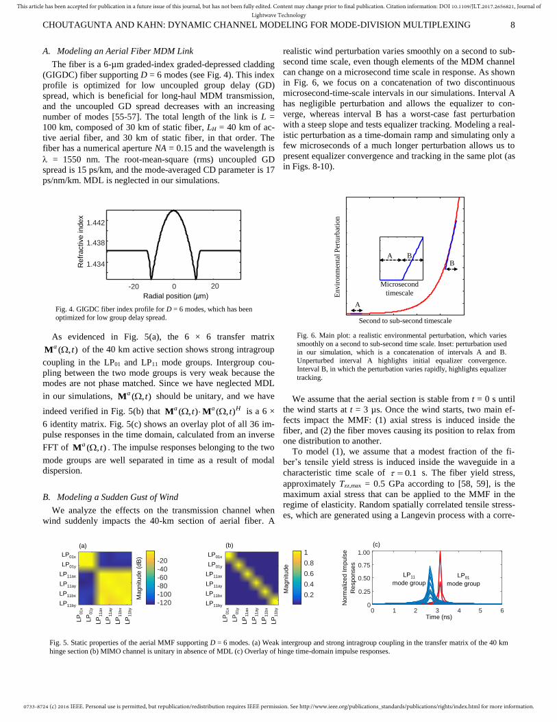
A. Modeling an Aerial Fiber MDM Link
The fiber is a 6-µm graded-index graded-depressed cladding
(GIGDC) fiber supporting D = 6 modes (see Fig. 4). This index
profile is optimized for low uncoupled group delay (GD)
spread, which is beneficial for long-haul MDM transmission,
and the uncoupled GD spread decreases with an increasing
number of modes [55-57]. The total length of the link is L =
100 km, composed of 30 km of static fiber, LH = 40 km of ac-
tive aerial fiber, and 30 km of static fiber, in that order. The
fiber has a numerical aperture NA = 0.15 and the wavelength is
= 1550 nm. The root-mean-square (rms) uncoupled GD
spread is 15 ps/km, and the mode-averaged CD parameter is 17
ps/nm/km. MDL is neglected in our simulations.
As evidenced in Fig. 5(a), the 6 × 6 transfer matrix
( , )a tM of the 40 km active section shows strong intragroup
coupling in the LP01 and LP11 mode groups. Intergroup cou-
pling between the two mode groups is very weak because the
modes are not phase matched. Since we have neglected MDL
in our simulations, ( , )a tM should be unitary, and we have
indeed verified in Fig. 5(b) that ( , ) ( , )a a Ht t M M is a 6 ×
6 identity matrix. Fig. 5(c) shows an overlay plot of all 36 im-
pulse responses in the time domain, calculated from an inverse
FFT of ( , )a tM . The impulse responses belonging to the two
mode groups are well separated in time as a result of modal
dispersion.
B. Modeling a Sudden Gust of Wind
We analyze the effects on the transmission channel when
wind suddenly impacts the 40-km section of aerial fiber. A
realistic wind perturbation varies smoothly on a second to sub-
second time scale, even though elements of the MDM channel
can change on a microsecond time scale in response. As shown
in Fig. 6, we focus on a concatenation of two discontinuous
microsecond-time-scale intervals in our simulations. Interval A
has negligible perturbation and allows the equalizer to con-
verge, whereas interval B has a worst-case fast perturbation
with a steep slope and tests equalizer tracking. Modeling a real-
istic perturbation as a time-domain ramp and simulating only a
few microseconds of a much longer perturbation allows us to
present equalizer convergence and tracking in the same plot (as
in Figs. 8-10).
We assume that the aerial section is stable from t = 0 s until
the wind starts at t = 3 µs. Once the wind starts, two main ef-
fects impact the MMF: (1) axial stress is induced inside the
fiber, and (2) the fiber moves causing its position to relax from
one distribution to another.
To model (1), we assume that a modest fraction of the fi-
ber’s tensile yield stress is induced inside the waveguide in a
characteristic time scale of 0.1 s. The fiber yield stress,
approximately Tzz,max = 0.5 GPa according to [58, 59], is the
maximum axial stress that can be applied to the MMF in the
regime of elasticity. Random spatially correlated tensile stress-
es, which are generated using a Langevin process with a corre-
Fig. 6. Main plot: a realistic environmental perturbation, which varies
smoothly on a second to sub-second time scale. Inset: perturbation used in our simulation, which is a concatenation of intervals A and B.
Unperturbed interval A highlights initial equalizer convergence.
Interval B, in which the perturbation varies rapidly, highlights equalizer
tracking.
A
BBA
Microsecond
timescale
Second to sub-second timescale
En
vir
on
men
tal P
ertu
rbat
ion
Fig. 5. Static properties of the aerial MMF supporting D = 6 modes. (a) Weak intergroup and strong intragroup coupling in the transfer matrix of the 40 km
hinge section (b) MIMO channel is unitary in absence of MDL (c) Overlay of hinge time-domain impulse responses.
0 1 2 3 4 5 60
0.25
0.50
0.75
1.00
Norm
aliz
ed Im
puls
e
Responses
Time (ns)
(c)
LP01x
LP01y
LP11ax
LP11ay
LP11bx
LP11by
LP
01x
LP
01y
LP
11ax
LP
11ay
LP
11b
x
LP
11b
y
LP01x
LP01y
LP11ax
LP11ay
LP11bx
LP11by
LP
01x
LP
01y
LP
11ax
LP
11ay
LP
11b
x
LP
11b
y
-120
-100
-80
-60
-40
-20
0.2
0.4
0.6
0.8
1
Magnitude (
dB
)
Magnitude
(b)(a)
LP11
mode group
LP01
mode group
Fig. 4. GIGDC fiber index profile for D = 6 modes, which has been
optimized for low group delay spread.
Radial position (µm)
-20 0 20
1.434
1.438
1.442
Refr
active index

0733-8724 (c) 2016 IEEE. Personal use is permitted, but republication/redistribution requires IEEE permission. See http://www.ieee.org/publications_standards/publications/rights/index.html for more information.
This article has been accepted for publication in a future issue of this journal, but has not been fully edited. Content may change prior to final publication. Citation information: DOI 10.1109/JLT.2017.2656821, Journal ofLightwave Technology
CHOUTAGUNTA AND KAHN: DYNAMIC CHANNEL MODELING FOR MODE-DIVISION MULTIPLEXING 9
lation length of 20 m, stretch the fiber. In the worst case, r =
1.5 × 10⁴ % of the yield stress is induced into the fiber. Since
the evolution of the wind is slow compared to the symbol rate
of the receiver, the induced stresses are modeled as time-
domain ramps. We again emphasize that the actual wind per-
turbation occurs on a sub-second time scale. The static interval
(interval A in Fig. 6) has a duration of 3 µs and the active in-
terval (interval B in Fig. 6) has a duration of 3 µs with a con-
stant slope of 4
, 1.5 10 0.5 GPa / 0.1 / % s 7500 Pa/s.zz maxrT (32)
Only a 6-µs time interval (3 µs of a stable channel followed by
3 µs of a dynamic channel) is studied in this paper because it is
sufficient to study channel dynamics and corresponding equal-
izer tracking behavior. The spatial distribution and time-
evolution of the axial stress is shown in Fig. 7. We note that
our perturbative modeling should be valid because the stress
magnitudes are very small.
To model (2), we assume that the fiber position shifts due to
contact between the fiber jacket and its surroundings. The local
curvatures of the MMF relax from one distribution to another
in the same time scale as stress because the fiber bends in re-
sponse to the wind. The initial curvatures,0 0( ) 1/ ( )z R z ,
are sampled from the positive part of a normal distribution with
a standard deviation of 1/2.5 m1. The curvatures 0.1 s later,
1( )z , are independently sampled from the same distribution.
The local curvature at each z during the wind gust is linearly
interpolated as
0 1 0( , ) ( ) ( ( ) ( )) ( / 0.1).z t z z z t (33)
Even though wind in a real setting might have additional ef-
fects beyond the simplified model we consider here, we show
in Subsection IV.D that our model reproduces expected chan-
nel dynamics behavior.
C. Adaptive MIMO Equalization
The end-to-end transfer Jones matrix )( ,tM represents
time-varying mode coupling and dispersion, necessitating the
use of an adaptive 6 × 6 MIMO equalizer W at the receiver.
For long-haul transmission, it is computationally efficient to
transmit a CP to represent the MDM channel as circular convo-
lution of discrete length sequences in the time-domain. This
operation corresponds to multiplication in the discrete frequen-
cy domain, which can be efficiently realized by FFT pro-
cessing in FDE. W approximately inverts M so the product
WM is approximately a 6 × 6 identity matrix. The convergence
properties of several adaptive FDE algorithms were previously
studied in [10]. Here, we focus on the tracking ability of the
least mean squares (LMS) algorithm. LMS uses stochastic gra-
dient descent to adapt to an unknown MIMO channel using
estimates of the equalizer error. Since the feedforward carrier-
recovery block has a delay of samples, we use delayed out-
puts to adapt the coefficients of the LMS equalizer2[60].
The coefficients of the 6 × 6 LMS equalizer at each discrete
frequency , 10,1, FFTk N are iteratively updated as [10,
61]
[ ] ( [ ] [ ] [ ]) [ ],[ ] Hk k k k kk W x W y yW (34)
where is a scalar step size,
1 6
-point FFT
of delayed ti
[ ] [ [
me d
], , [
omain signals
]
[ ]
] T
FFT
k X k X k
N
n
x
x
(35)
is a block of known or estimated frequency domain data sym-
bols that were transmitted,
1 6
-point FFT
[ ] [ ] [ ] [ ]
of de
[ [ ], , [ ]]
layed time domain signals [ ]
T
FFT
k k k k
Y k Y k
N
n
y
y M x n
(36)
is a block of received frequency-domain symbols at the input
of the equalizer, and 1 6[ ] [ [ ], , [ ]]Tk N k N k n is a block of
noise samples. The convergence rate and performance of the
LMS algorithm depend on the choice of which must satisfy
the convergence criterion 2 /0 max . Here max is the
largest eigenvalue of the autocovariance matrix of [ ]ky ,
[ ] [ ] [ ]Hk ER k ky y y [10] . The squared error in the equal-
ized samples at each discrete frequency k is computed as 22[ ] [ ] [ ] [ ]k k k k x W y , and we compute a normalized
mean-squared error (MSE) by ensemble averaging the squared
error over all NFFT discrete-frequencies, all modes, and many
realizations of the transmitted data symbols [ ]nx .
2 Lasers currently used in telecommunications have linewidths of the order
of hundreds of kHz. Feedforward carrier recovery, often used for carrier phase recovery, employs filtering to average phase noise estimates. This filtering
introduces a delay of tens to hundreds of samples (corresponding to several
nanoseconds) between the equalizer outputs and computation of the error sig-nals used to train the equalizer coefficients. The channel changes on a micro-
second time scale, and our simulations show that the delay causes a negligi-
ble increase in the equalizer MSE. All plots in this paper assume Δ = 0 for simplicity.
Fig. 7. Spatial and temporal distribution of the induced axial stress due to wind. Only 1 km active section is shown.
0 0.25 0.50 0.75 1.00
6.0
4.5
3.0
1.5
00
0.05
0.1
Tim
e (
µs)
Str
ess (
Pa)
Fiber Position (km)

0733-8724 (c) 2016 IEEE. Personal use is permitted, but republication/redistribution requires IEEE permission. See http://www.ieee.org/publications_standards/publications/rights/index.html for more information.
This article has been accepted for publication in a future issue of this journal, but has not been fully edited. Content may change prior to final publication. Citation information: DOI 10.1109/JLT.2017.2656821, Journal ofLightwave Technology
CHOUTAGUNTA AND KAHN: DYNAMIC CHANNEL MODELING FOR MODE-DIVISION MULTIPLEXING 10
In our simulation, both polarizations of the LP01 and LP11
mode groups are launched at the transmitter and all six modes
are detected with a coherent MIMO receiver which is operating
at a symbol rate of Rs = 20 Gbaud. Random quadrature phase-
shift keying training data [ ]nx is sent on each mode and
[ ]ny is detected at a signal-to-noise ratio (SNR) of 15 dB.
The SNR is defined as the received signal power over all six
modes divided by the received noise power per mode. The
LMS equalizer has a step size of 0.05 and a FFT block
size of 92FFTN .
D. Simulation Results of Aerial Fiber Dynamics
We now study the channel dynamics of the aerial fiber link
and tracking performance of LMS-adapted MIMO FDE, and
their dependence on the strength of the wind perturbation,
number of modes, and the length of the hinge. In each compar-
ison, the default parameters are D = 6 modes and hinge length
is LH = 40 km. The default wind perturbation stretches the fiber
from 0% to 1.5 × 10⁴% of the yield strength and shifts the
local curvatures from one distribution to another in 0.1 s. The
LMS algorithm step size is fixed at µ = 0.05 and the block size 92FFTN for all cases considered here.
Figs. 8-10 (a)-(c) show the evolution of elements in the re-
ceived Jones vector at the carrier frequency [ 0]k y when a
fixed Jones vector [ 0]k x is transmitted. The elements of y
remain stable until t = 3 µs, when the wind perturbation is
turned on. Increasing axial stress and shifting curvatures cause
time-varying mode coupling, as evidenced by change in the
received Jones vector elements. Even though the wind pertur-
bation happens only in the sub-second time scale, we observe
microsecond-time-scale channel dynamics, consistent with
initial experimental observations [6]. The equalizer starts with-
out an initial estimate of the fiber channel and so its weights
are initialized to 0 at t = 0 s. The equalizer begins learning the
static fiber channel and its weights converge to the optimum
values around t = 1.5 µs. When the wind starts, the equalizer
changes from convergence mode to tracking mode. Its weights
track the time-varying modal dispersion and mode coupling as
a function of the scalar step size µ (discussed further in Sub-
section IV.E). The evolution of the diagonal coefficients of the
MIMO equalizer are shown in Figs. 8-10 (d)-(f). For clarity,
only the diagonal weights of the equalizer are shown. Figs. 8-
10 (g) show equalizer learning performance in terms of nor-
malized MSE during initial convergence and subsequent track-
ing.
Fig. 8 shows the channel dynamics and equalizer tracking
behavior when the strength of the wind acting on the aerial
fiber is varied. The wind perturbations in Figs. 8(b), (e) and
Figs. 8(c), (f) are two and four times as strong as in Figs. 8(a),
(d), respectively. As expected, the received Jones vector ele-
ments evolve faster with increasing perturbation strength. The
LMS equalizer converges around t = 1.5 µs for all three cases,
yielding an asymptotic normalized MSE around 0.01. When
the wind starts at t = 3 µs, the channels become dynamic and
the instantaneous normalized MSE increases to 0.03, 0.07, and
0.21 for the three wind strengths, suggesting a super-linear
scaling of the MSE with the strength of perturbation.
Fig. 9 shows how the channel dynamics and equalizer track-
ing performance change when D is varied. The received Jones
vector elements of an aerial cable using MMF (D = 6, 12)
evolve faster than those of an aerial cable using SMF (D = 2).
As the dimensionality of the system increases, the complex
dynamics of mode coupling and dispersion make it more diffi-
cult for the equalizer to track the MIMO channel, as evidenced
by the higher instantaneous MSE for MMFs as compared to
SMF, which is shown in Fig. 9(g).
While MMF channels have been observed to change faster
than SMF channels, as shown in [6] and later references, the
underlying physical reasons for the increased rate of change are
not entirely clear. Within our model based on coupled-mode
theory, it is the matrices ,t) and K,t), which appear in
the exponent of the transfer matrix M,t) (see, e.g., (14)), that
are responsible for all linear effects. As D increases, a given
external force causes the pairwise coupling coefficients in
Kd,t) to change faster; higher-order modes tend to overlap
more than lower-order modes, so the overlap integrals describ-
ing the pairwise coupling coefficients are more sensitive to
changes in the index perturbation. While this reasoning is not
yet validated experimentally, the predictions of our model are
consistent with experimental observations.
Fig. 10 shows a similar comparison, namely, how the chan-
nel dynamics and equalizer tracking performance change when
the length of the aerial fiber exposed to the wind is varied. As
expected, longer exposed fiber lengths cause faster channel
dynamics, because the end-to-end Jones transfer matrix repre-
sents the cumulative effects of local mode coupling and disper-
sion integrated along the fiber length. Consequently, tracking
dynamic channels with longer fiber lengths can yield higher
instantaneous MSE, as shown in Fig. 10(g).
Figs. 8-10 empirically show the effect of varying different
parameters on MDM channel dynamics and the output MSE of
the equalizer. It is of significant practical interest to develop
insightful metrics to quantify the rate of change of a MIMO
channel, explain their dependence on system parameters, and
establish a connection to the output MSE of the adaptive
MIMO equalizer.
Channel dynamics in SMF, with D = 2 modes, are often de-
scribed in terms of rotations per second of the received Stokes
vector on the Poincaré sphere. In these low-dimensional sys-
tems, higher rotation rates are correlated with increased diffi-
culty of tracking by an adaptive equalizer. Moreover, the rota-
tion rate is easy to measure using polarimeters in a laboratory
setting, and consequently this metric has become the optical
communications industry’s de facto metric for quantifying
channel rate of change. However, a simple extension of this
idea for D > 2 modes to rotations of the generalized Stokes
vector on the generalized Poincaré sphere can be non-physical.
Not all vectors on the generalized Poincaré sphere have a legit-
imate representation as a generalized Jones vector [16]. More-
over, generalized Stokes vectors are constructed from their
generalized Jones vector counterparts using trace-orthogonal
basis Pauli matrices, which are not unique.

0733-8724 (c) 2016 IEEE. Personal use is permitted, but republication/redistribution requires IEEE permission. See http://www.ieee.org/publications_standards/publications/rights/index.html for more information.
This article has been accepted for publication in a future issue of this journal, but has not been fully edited. Content may change prior to final publication. Citation information: DOI 10.1109/JLT.2017.2656821, Journal ofLightwave Technology
CHOUTAGUNTA AND KAHN: DYNAMIC CHANNEL MODELING FOR MODE-DIVISION MULTIPLEXING 11
Fig. 9. Received Jones vector elements for a random transmitted Jones vector and LMS equalizer diagonal taps with µ = 0.05 when the axial stress is
ramped from 0% to 1.5 × 10⁻⁴ % of fiber yield strength and local curvatures are changing within 0.1 seconds for (a)(d) D = 2 modes, (b)(e) D = 6 modes and
(c)(f) D = 12 modes. The corresponding MSE curves are shown in (g).
-1
-0.5
0
0.5
1
Real
Imag
-1
-0.5
0
0.5
1
Real
Imag
-1
-0.5
0
0.5
1
Real
Imag
-1
-0.5
0
0.5
1
Real
Imag
-1
-0.5
0
0.5
1
Real
Imag
-1
-0.5
0
0.5
1
Real
Imag
0
0.25
0.5
0.75
1
0 1.5 3.0 4.5 6.0
0 1.5 3.0 4.5 6.00 1.5 3.0 4.5 6.0
0 1.5 3.0 4.5 6.0
0 1.5 3.0 4.5 6.0
0 1.5 3.0 4.5 6.0
0 1.5 3.0 4.5 6.0
Recd.
Jones
Ele
ments
Recd.
Jones
Ele
ments
Recd.
Jones
Ele
ments
Equaliz
er
Taps
Equaliz
er
Taps
Equaliz
er
Taps
Time (µs) Time (µs) Time (µs)
Norm
aliz
ed M
ean S
quare
d E
rror
(a)
(b)
(c)
(d)
(e)
(f)
(g)
D = 2D = 6
D = 12
Fig. 8. Received Jones vector elements for a random transmitted Jones vector for D = 6 modes, LMS equalizer diagonal taps with µ = 0.05 when the axial
stress is ramped from (a)(d) 0% to 1.5 × 10⁻⁴ %, (b)(e) 0% to 3 × 10⁻⁴ %, and (c)(f) 0% to 6 × 10⁻⁴ % of fiber yield stress within 0.1 seconds. The distribution
of curvatures in (b)(e) and (c)(f) is changing two times and four times faster than in (a)(d), respectively. The corresponding MSE curves are shown in (g).
-1
-0.5
0
0.5
1
Real
Imag
-1
-0.5
0
0.5
1
Real
Imag
-1
-0.5
0
0.5
1
Real
Imag
0 1.5 3.0 4.5 6.0-1
-0.5
0
0.5
1
Real
Imag
-1
-0.5
0
0.5
1
Real
Imag
-1
-0.5
0
0.5
1
Real
Imag
0 1.5 3.0 4.5 6.00
0.25
0.5
0.75
1
0 1.5 3.0 4.5 6.0
0 1.5 3.0 4.5 6.0
0 1.5 3.0 4.5 6.0
0 1.5 3.0 4.5 6.0
0 1.5 3.0 4.5 6.0
Recd.
Jones
Ele
ments
Recd.
Jones
Ele
ments
Recd.
Jones
Ele
ments
Equaliz
er
Taps
Equaliz
er
Taps
Equaliz
er
Taps
Time (µs) Time (µs) Time (µs)
Norm
aliz
ed M
ean S
quare
d E
rror
0% - 1.5×10⁻⁴ %
0% - 3×10⁻⁴ %
0% - 6×10⁻⁴ %
(a)
(b)
(c)
(d)
(e)
(f)
(g)

0733-8724 (c) 2016 IEEE. Personal use is permitted, but republication/redistribution requires IEEE permission. See http://www.ieee.org/publications_standards/publications/rights/index.html for more information.
This article has been accepted for publication in a future issue of this journal, but has not been fully edited. Content may change prior to final publication. Citation information: DOI 10.1109/JLT.2017.2656821, Journal ofLightwave Technology
CHOUTAGUNTA AND KAHN: DYNAMIC CHANNEL MODELING FOR MODE-DIVISION MULTIPLEXING 12
Given these complications, it is hard to relate rotations on the
generalized Poincaré sphere to output MSE of the adaptive
MIMO equalizer. Nevertheless, determining if rotation rate of
the generalized Stokes vector has useful meaning or develop-
ing other, more useful, metrics to quantity the rate of MDM
channel change is an important subject for future research.
E. Optimization of LMS Equalization Algorithm Parameters
The tracking performance of the LMS FDE algorithm is a
strong function of its step size and FFT block length. In this
section, we vary these parameters to study the effect on the
instantaneous MSE.
The choice of µ has an important system design tradeoff: it
should be chosen large enough to allow the weights to faithful-
ly track dynamic channels, but small enough to avoid excess
mean squared error (MSE) in stable channels. As shown in Fig.
11, small values for µ yield the smallest asymptotic MSE when
the channel is stable but result in slow tracking of channel dy-
namics. High values for µ result in excess MSE when the link
is stable due to noisy equalizer updates but are capable of
tracking dynamics faithfully [62]. Considering this tradeoff,
0.05 is a reasonable choice for the example system con-
sidered here. In practice, µ is often adjusted empirically to op-
timize performance.
Since the LMS-adapted FDE is iteratively updated using
received blocks of NFFT samples of D × 1 vectors, successive
LMS updates must equalize changes to the Jones transfer ma-
trix that have occurred in the past NFFT samples. The change to
the transfer matrix that is seen by the equalizer is proportional
to both the rate of channel dynamics and NFFT, which means
that the tracking ability of the equalizer is reduced as NFFT is
increased. However, long-haul MDM systems have a large
group delay spread, which requires a large CP. The require-
ment of a high CP efficiency to increase throughput puts a
lower bound on the NFFT that can be employed.
V. CONCLUSIONS
We have extended the multi-section model to describe how
spatial- and polarization- mode coupling in MMFs change in
response to fast environmental perturbations. Our model is able
to compute the time-varying Jones transfer matrix of an end-to-
end MDM link when given the distributions of the environ-
mental perturbations that are acting upon it. The essence of our
model is to assume that a MMF has built-in defects originating
from manufacturing and cabling that reproduce the expected
behavior of mode coupling and dispersion when the link is
stable.
The driving environmental perturbations, including axial
stress, curvature and external electromagnetic fields, modulate
the fiber properties to produce time-varying mode-dependent
Fig. 11. Tracking performance of the LMS FDE algorithm for various
values of the step size parameter µ. Over a time interval of 0.1 s, the axial stress is ramped from 0% to 1.5 × 10⁻⁴ % of fiber yield strength and the
local curvatures are changed. The MMF supports D = 6 modes and the
length of the aerial hinge is LH = 40 km.
00 1 2 3 4 5 6
0.2
0.4
0.6
0.8
1.0
µ = 0.02
µ = 0.2
µ = 0.1
µ = 0.05
Norm
aliz
ed M
ean S
quare
d E
rror
Time (µs)
Fig. 10. Received Jones vector elements for a random transmitted Jones vector for D = 6 modes and LMS equalizer diagonal taps with µ = 0.05 when the axial stress is ramped from 0% to 1.5 × 10⁻⁴ % of fiber yield strength and local curvatures are changing within 0.1 seconds for hinge length (a)(d) LH = 40
km, (b)(e) LH = 100 km and (c)(f) LH = 160 km. The corresponding MSE curves are shown in (g).
-1
-0.5
0
0.5
1
Real
Imag
-1
-0.5
0
0.5
1
Real
Imag
-1
-0.5
0
0.5
1
Real
Imag
-1
-0.5
0
0.5
1
Real
Imag
-1
-0.5
0
0.5
1
Real
Imag
-1
-0.5
0
0.5
1
Real
Imag
0
0.25
0.5
0.75
1
0 1.5 3.0 4.5 6.0
0 1.5 3.0 4.5 6.00 1.5 3.0 4.5 6.0
0 1.5 3.0 4.5 6.0
0 1.5 3.0 4.5 6.0
0 1.5 3.0 4.5 6.0
0 1.5 3.0 4.5 6.0
Recd.
Jones
Ele
ments
Recd.
Jones
Ele
ments
Recd.
Jones
Ele
ments
Equaliz
er
Ta
ps
Equaliz
er
Ta
ps
Equaliz
er
Ta
ps
Time (µs) Time (µs) Time (µs)
Norm
aliz
ed M
ean S
quare
d E
rror
(a)
(b)
(c)
(d)
(e)
(f)
(g)
LH = 40 km
LH = 100 km
LH = 160 km

0733-8724 (c) 2016 IEEE. Personal use is permitted, but republication/redistribution requires IEEE permission. See http://www.ieee.org/publications_standards/publications/rights/index.html for more information.
This article has been accepted for publication in a future issue of this journal, but has not been fully edited. Content may change prior to final publication. Citation information: DOI 10.1109/JLT.2017.2656821, Journal ofLightwave Technology
CHOUTAGUNTA AND KAHN: DYNAMIC CHANNEL MODELING FOR MODE-DIVISION MULTIPLEXING 13
phase shifts, mode coupling, and modal dispersion in a dynam-
ic channel. We have shown that the rate of channel dynamics
can be in the microsecond time scale even though the time
scale for the environmental dynamics is much slower, e.g., on
the sub-second time scale. The MDM channel evolves faster as
D is increased because external forces can potentially impose
stronger and faster changes to the mode coupling coefficient
matrix. Increasing the hinge length of an MDM link also in-
creases the rate of dynamics because distributed perturbations
can interact with the channel over a longer length.
The increased speed of channel dynamics with increasing
number of modes D or link length can potentially have a criti-
cal impact on adaptive MIMO equalization in long-haul MDM
systems. Adaptive equalizers need to be designed so that they
can track the fastest channel variations. However, there is an
inherent tradeoff in the tracking ability in dynamic channels
and the asymptotic MSE in static channels. The long group-
delay spread necessitates a large CP length, and a high CP effi-
ciency requires a large FFTN , but large FFTN slows down
equalizer tracking and lead to higher MSE when the channel
changes rapidly.
REFERENCES
[1] T. Morioka, et al., "Enhancing optical communications with brand new
fibers," IEEE Commun. Mag., vol. 50, pp. s31-s42, 2012.
[2] E. Ip, G. Milione, Y.-K. Huang, and T. Wang, "Impact of mode-dependent loss on long-haul transmission systems using few-mode
fibers," in Proc. OFC, 2016.
[3] P. M. Krummrich and K. Kotten, "Extremely fast (microsecond timescale) polarization changes in high speed long haul WDM
transmission systems," in Proc. OFC, 2004.
[4] K. Roberts, et al., "Performance of dual-polarization QPSK for optical transport systems," J. Lightw. Technol., vol. 27, pp. 3546-3559, 2009.
[5] M. Boroditsky, et al., "Polarization dynamics in installed fiberoptic
systems," in Proc. IEEE LEOS Annu. Meeting, 2005, pp. 414-415.
[6] X. Chen, et al., "Characterization and analysis of few-mode fiber channel
dynamics," IEEE Photon. Technol. Lett., vol. 25, pp. 1819-1822, 2013.
[7] K. Ogaki, M. Nakada, Y. Nagao, and K. Nishijima, "Fluctuation differences in the principal states of polarization in aerial and buried
cables," in Proc. OFC, 2003.
[8] M. Brodsky, et al., "Physical mechanism for polarization mode dispersion temporal dynamics," IEEE LEOS Newslett., 2004.
[9] K. Choutagunta and J. M. Kahn, "Dynamic channel modeling for mode-division multiplexing," in Proc. IEEE Photon. Soc. Summer Topical
Space-Division Multiplex. and Multimode Photon., Newport Beach, CA,
USA, July 11-13, 2016, pp. 49-50. [10] S. Ö. Arık, D. Askarov, and J. M. Kahn, "Adaptive frequency-domain
equalization in mode-division multiplexing systems," J. Lightw. Technol.,
vol. 32, pp. 1841-1852, 2014. [11] S. Ö. Arik, D. Askarov, and J. M. Kahn, "Effect of mode coupling on
signal processing complexity in mode-division multiplexing," J. Lightw.
Technol., vol. 31, pp. 423-431, 2013. [12] C. D. Poole, "Statistical treatment of polarization dispersion in single-
mode fiber," Opt. Lett., vol. 13, pp. 687-689, 1988.
[13] C. D. Poole and R. E. Wagner, "Phenomenological approach to polarisation dispersion in long single-mode fibres," Electron. Lett., vol.
22, pp. 1029-1030, 1986.
[14] J. P. Gordon and H. Kogelnik, "PMD fundamentals: Polarization mode dispersion in optical fibers," Proc. Natl. Acad. Sci., vol. 97, pp. 4541-
4550, 2000.
[15] C. Antonelli, A. Mecozzi, M. Shtaif, and P. J. Winzer, "Random coupling between groups of degenerate fiber modes in mode multiplexed
transmission," Opt. Exp., vol. 21, pp. 9484-9490, 2013.
[16] C. Antonelli, A. Mecozzi, M. Shtaif, and P. J. Winzer, "Stokes-space analysis of modal dispersion in fibers with multiple mode transmission,"
Opt. Exp., vol. 20, pp. 11718-11733, 2012.
[17] J. Schuster, Z. Marzec, W. L. Kath, and G. Biondini, "Hybrid hinge
model for polarization-mode dispersion in installed fiber transmission systems," J. Lightw. Technol., vol. 32, pp. 1412-1419, 2014.
[18] J. Li, G. Biondini, W. L. Kath, and H. Kogelnik, "Anisotropic hinge
model for polarization-mode dispersion in installed fibers," Opt. Lett., vol. 33, pp. 1924-1926, 2008.
[19] J. Li, G. Biondini, W. L. Kath, and H. Kogelnik, "Outage statistics in a
waveplate hinge model of polarization-mode dispersion," J. Lightw. Technol., vol. 28, pp. 1958-1968, 2010.
[20] C. Antonelli and A. Mecozzi, "Theoretical characterization and system
impact of the hinge model of PMD," J. Lightw. Technol., vol. 24, pp. 4064-4074, 2006.
[21] D. S. Waddy, L. Chen, and X. Bao, "Theoretical and experimental study
of the dynamics of polarization-mode dispersion," IEEE Photon. Technol. Lett., vol. 14, pp. 468-470, 2002.
[22] A. Mecozzi, C. Antonelli, M. Boroditsky, and M. Brodsky,
"Characterization of the time dependence of polarization mode dispersion," Opt. Lett., vol. 29, pp. 2599-2601, 2004.
[23] C. B. Czegledi, M. Karlsson, E. Agrell, and P. Johannisson, "Polarization
drift channel model for coherent fibre-optic systems," Scientific Reports, vol. 6, p. 21217, 2016.
[24] M. Brodsky, N. J. Frigo, M. Boroditsky, and M. Tur, "Polarization mode
dispersion of installed fibers," J. Lightw. Technol., vol. 24, pp. 4584-4599, 2006.
[25] G. Soliman, "Temporal dynamics of polarization and polarization mode
dispersion and influence on optical fiber systems," Ph.D. dissertation, University of Waterloo, 2013.
[26] R. Roberge, "Case study: PMD measurement on aerial fiber under wind-induced oscillations and vibration," 2009. [Online]. Available:
http://metrotek.ru/
[27] M. Belloli, A. Collina, and F. Resta, "Cables vibration due to wind action," 2006. [Online]. Available: http://www.oitaf.org/
[28] M. Kurono, K. Isawa, and M. Kuribara, "Transient state of polarization in
optical ground wire caused by lightning and impulse current," in Proc. Proc. SPIE, pp. 242-245.
[29] S. M. Pietralunga, J. Colombelli, A. Fellegara, and M. Martinelli, "Fast
polarization effects in optical aerial cables caused by lightning and impulse current," IEEE Photon. Technol. Lett., vol. 16, pp. 2583-2585,
2004.
[30] J. G. Rose, D. M. Durrett, L. A. Walker, and J. C. Stith, "Highway-railway at-grade crossings: trackbed and surface pressure measurements
and assessments," 2009. [Online]. Available: http://uknowledge.uky.edu/
[31] T. G. Gutowski and C. L. Dym, "Propagation of ground vibration: a review," J. Sound and Vibration, vol. 49, pp. 179-193, 1976.
[32] M. Brodsky, J. C. Martinez, N. J. Frigo, and A. Sirenko, "Dispersion
compensation module as a polarization hinge," in Proc. ECOC, Sep. 2005, pp. 335-336.
[33] Cisco, "Data center power and cooling," [Online]. Available:
http://www.cisco.com/ [34] D. Marcuse, Theory of dielectric optical waveguides, 2nd ed. New York:
Academic Press, 1991.
[35] J. N. Damask, Polarization optics in telecommunications. New York: Springer-Verlag, 2005.
[36] J. Proakis and M. Salehi, Digital Communications, 5 ed. New York, NY,
USA: McGraw-Hill, 2007. [37] R. Olshansky, "Mode coupling effects in graded-index optical fibers,"
Appl. Opt., vol. 14, pp. 935-945, 1975.
[38] S. Ö. Arık and J. M. Kahn, "Coupled-core multi-core fibers for spatial multiplexing," IEEE Photon. Technol. Lett., vol. 25, pp. 2054-2057,
2013.
[39] C.-L. Chen, Foundations for guided-wave optics. New York: Wiley-Interscience, 2006.
[40] A. Li, Y. Wang, Q. Hu, and W. Shieh, "Few-mode fiber based optical
sensors," Opt. Exp., vol. 23, pp. 1139-1150, 2015. [41] T. Hayashi, et al., "Crosstalk variation of multi-core fibre due to fibre
bend," in Proc. ECOC, 2010, pp. 1-3.
[42] H. Bülow, H. Al-Hashimi, B. T. Abebe, and B. Schmauss, "Capacity and outage of multimode fiber with statistical bends," in Proc. OFC/NFOEC,
2012, pp. 1-3.
[43] A. A. Juarez, et al., "Modeling of mode coupling in multimode fibers with respect to bandwidth and loss," J. Lightw. Technol., vol. 32, pp.
1549-1558, 2014.
[44] P. M. Krummrich, et al., "Demanding response time requirements on coherent receivers due to fast polarization rotations caused by lightning
events," Opt. Exp., vol. 24, pp. 12442-12457, 2016.
0733-8724 (c) 2016 IEEE. Personal use is permitted, but republication/redistribution requires IEEE permission. See http://www.ieee.org/publications_standards/publications/rights/index.html for more information.
This article has been accepted for publication in a future issue of this journal, but has not been fully edited. Content may change prior to final publication. Citation information: DOI 10.1109/JLT.2017.2656821, Journal ofLightwave Technology
CHOUTAGUNTA AND KAHN: DYNAMIC CHANNEL MODELING FOR MODE-DIVISION MULTIPLEXING 14
[45] J. Wuttke, P. M. Krummrich, and J. Rosch, "Polarization oscillations in
aerial fiber caused by wind and power-line current," IEEE Photon. Technol. Lett., vol. 15, pp. 882-884, 2003.
[46] M. Brodsky, P. Magill, and N. J. Frigo, "Polarization-mode dispersion of
installed recent vintage fiber as a parametric function of temperature," IEEE Photon. Technol. Lett., vol. 16, pp. 209-211, 2004.
[47] R. Ulrich and A. Simon, "Polarization optics of twisted single-mode
fibers," Appl. Opt., vol. 18, pp. 2241-2251, 1979. [48] L. Palmieri and A. Galtarossa, "Coupling effects among degenerate
modes in multimode optical fibers," IEEE Photon. J., vol. 6, pp. 1-8,
2014. [49] M. V. Berry, "Interpreting the anholonomy of coiled light," Nature, vol.
326, pp. 277-278, 1987.
[50] M. V. Berry, "The adiabatic phase and Pancharatnam's phase for polarized light," J. Mod. Opt., vol. 34, pp. 1401-1407, 1987.
[51] M. Plöschner, T. Tyc, and T. Čižmár, "Seeing through chaos in
multimode fibres," Nat. Photon., vol. 9, pp. 529-535, 2015. [52] J. N. Blake, S. Y. Huang, B. Y. Kim, and H. J. Shaw, "Strain effects on
highly elliptical core two-mode fibers," Opt. Lett., vol. 12, pp. 732-734,
1987. [53] R. Ulrich, S. C. Rashleigh, and W. Eickhoff, "Bending-induced
birefringence in single-mode fibers," Opt. Lett., vol. 5, pp. 273-275,
1980. [54] S. Rashleigh, "Origins and control of polarization effects in single-mode
fibers," J. Lightw. Technol., vol. 1, pp. 312-331, 1983.
[55] D. Donlagic, "Opportunities to enhance multimode fiber links by application of overfilled launch," J. Lightw. Technol., vol. 23, pp. 3526-
3540, 2005. [56] K. Okamoto and T. Okoshi, "Computer-aided synthesis of the optimum
refractive-index profile for a multimode fiber," IEEE Trans. Microw.
Theory Tech., vol. MTT-25, pp. 213-221, 1977. [57] K. Takahashi, T. Ishigure, and Y. Koike, "Index profile design for high-
bandwidth W-shaped plastic optical fiber," J. Lightw. Technol., vol. 24,
pp. 2867-2876, 2006. [58] Corning Inc., "Corning SMF-28 optical fiber," datasheet, 2002.
[59] R. Romaniuk, "Tensile strength of tailored optical fibers," Opto-Electron.
Rev., pp. 101-116, 2000. [60] E. Ip and J. M. Kahn, "Feedforward carrier recovery for coherent optical
communications," J. Lightw. Technol., vol. 25, pp. 2675-2692, 2007.
[61] S. Randel, et al., "6×56-Gb/s mode-division multiplexed transmission over 33-km few-mode fiber enabled by 6×6 MIMO equalization," Opt.
Exp., vol. 19, pp. 16697-16707, 2011.
[62] B. Widrow and S. D. Stearns, Adaptive signal processing. New Jersey: Prentice-Hall, 1985.
Karthik Choutagunta (S’11) received the B.S. degree from
The University of Texas at Austin in 2014, and the M.S. degree
from Stanford University in electrical engineering in 2016. He
is currently working towards the Ph.D. degree at Stanford Uni-
versity. He worked at Coherent Logix (Austin, TX, USA) in
summer 2012, at Intel Corp. (Austin, TX, USA) from 2012-
2014, and at Apple Inc. (Cupertino, CA, USA) in fall 2015 and
summer 2016. His main current research interests include vari-
ous topics in optical communications, wireless communica-
tions, and signal processing.
Joseph M. Kahn (M’90–SM’98–F’00) received the A.B.,
M.A., and Ph.D. degrees in physics from U.C. Berkeley in
1981, 1983, and 1986, respectively. From 1987–1990, he was
at AT&T Bell Laboratories, Crawford Hill Laboratory, in
Holmdel, NJ, USA. He demonstrated multi-Gbit/s coherent
optical fiber transmission systems, setting world records for
receiver sensitivity. From 1990–2003, he was with the Faculty
of the Department of Electrical Engineering and Computer
Sciences at U.C. Berkeley, performing research on optical and
wireless communications. Since 2003, he has been a Professor
of Electrical Engineering at Stanford University, where he
heads the Optical Communications Group. His current research
interests include fiber-based imaging, spatial multiplexing,
rate-adaptive and spectrally efficient modulation and coding
methods, coherent detection and associated digital signal pro-
cessing algorithms, digital compensation of fiber nonlinearity,
and free-space systems. He received the National Science
Foundation Presidential Young Investigator Award in 1991.
From 1993–2000, he served as a technical editor of IEEE Per-
sonal Communications Magazine. Since 2009, he has been an
Associate Editor of IEEE/OSA Journal of Optical Communica-
tions and Networking. In 2000, he helped found StrataLight
Communications, where he served as Chief Scientist from
2000–2003. StrataLight was acquired by Opnext, Inc., in 2009.


![Introduction... · Web viewThe channel name used for this dynamic virtual channel is "TSMF". The usage of a channel name when opening a dynamic virtual channel is specified in [MS-RDPEDYC]](https://img.pdfslide.us/doc/110x75/5fcda61244204d6e925df440/introduction-web-view-the-channel-name-used-for-this-dynamic-virtual-channel.jpg)