Embed Size (px)
Citation preview
7/30/2019 Dynamic CDynamic crack propagation based on loss of hyperbolicity and a new discontimuous enrichmentrack Pr…
http://slidepdf.com/reader/full/dynamic-cdynamic-crack-propagation-based-on-loss-of-hyperbolicity-and-a-new 1/33
INTERNATIONAL JOURNAL FOR NUMERICAL METHODS IN ENGINEERINGInt. J. Numer. Meth. Engng 2003; 58:1873–1905 (DOI: 10.1002/nme.941)
Dynamic crack propagation based on loss of hyperbolicity
and a new discontinuous enrichment
Ted Belytschko∗;†, Hao Chen1; 2, Jingxiao Xu1 and Goangseup Zi1
1Department of Mechanical Engineering; Northwestern University; 2145 Sheridan Road ;Evanston; IL 60208-3111; U.S.A.
2Livermore Software Technology Corporation; 7374 Las Positas Road ; Livermore; CA 94550; U.S.A.
SUMMARY
A methodology is developed for switching from a continuum to a discrete discontinuity where thegoverning partial dierential equation loses hyperbolicity. The approach is limited to rate-independentmaterials, so that the transition occurs on a set of measure zero. The discrete discontinuity is treated bythe extended ÿnite element method (XFEM) whereby arbitrary discontinuities can be incorporated inthe model without remeshing. Loss of hyperbolicity is tracked by a hyperbolicity indicator that enables both the crack speed and crack direction to be determined for a given material model. A new methodwas developed for the case when the discontinuity ends within an element; it facilitates the modelling of crack tips that occur within an element in a dynamic setting. The method is applied to several dynamiccrack growth problems including the branching of cracks. Copyright ? 2003 John Wiley & Sons, Ltd.
KEY WORDS: ÿnite element method; fracture mechanics; dynamic fracture; loss of hyperbolicity;cohesive crack model; extended ÿnite element method
1. INTRODUCTION
It is well known that the loss of hyperbolicity, i.e. a change of type of the momentumequations for a rate-independent material leads to a localization of deformation to a set of measure zero. In Bazant and Belytschko [1], a closed form solution was obtained for the one-dimensional case for a rate-independent material and it was shown that the strain becomes aDirac delta function at the ÿrst point where hyperbolicity is lost, i.e. at the point where thetangent modulus loses its positive slope; material behaviour with a negative tangent modulusis often called strain softening. As a consequence, the displacement ÿeld develops a discon-tinuity, i.e. the material separates, at this point. Although this change of type of the partialdierential equation is often called ill-posedness, this characterization is controversial since a
∗Correspondence to: Ted Belytschko, Department of Mechanical Engineering, Northwestern University, 2145Sheridan Road, Room A212, Evanston, IL 60208-3111, U.S.A.
†E-mail: [email protected]
Contract= grant sponsor: Oce of Naval Research
Received 14 February 2003
Revised 12 March 2003Copyright ? 2003 John Wiley & Sons, Ltd. Accepted 3 July 2003
7/30/2019 Dynamic CDynamic crack propagation based on loss of hyperbolicity and a new discontimuous enrichmentrack Pr…
http://slidepdf.com/reader/full/dynamic-cdynamic-crack-propagation-based-on-loss-of-hyperbolicity-and-a-new 2/33
1874 T. BELYTSCHKO ET AL.
solution can be obtained after loss of hyperbolicity. However, the continuation of the solutionrequires additional models because the displacement discontinuity is developed without thedissipation of any energy [1, 2]. Thus if we consider the separation process to be fracture,modelling it by a rate-independent material with strain softening without transition to an in-
terface model that can dissipate energy is inappropriate as a model for the physical process of cracking.
In this paper, we consider the treatment of the fracture process by introducing a discretediscontinuity wherever the partial dierential equation changes type. Across this discontinuity,a traction-displacement law, i.e. a cohesive law, is imposed. The energy dissipation acrossthe discontinuity is chosen to match the energy of fracture. The direction and velocity of the
propagation of fracture are directly determined by the loss of hyperbolicity criterion. Thus themethod is capable of providing the crack speed and direction from the material model. Thetransition from continuum to discrete separation in an element is implemented through theextended ÿnite element method (XFEM), which permits arbitrary discontinuities to be addedto a ÿnite element mesh without remeshing via discontinuous partitions of unity.
Another class of fracture methods are the inter-element models with cohesive laws, Xu and Needleman [3], Camacho and Ortiz [4] and Ortiz and Pandolÿ [5]; (these are often calledcohesive models but the name is misleading since cohesive fracture laws can be implementedin many methods, such as the XFEM implementation described here). These models havesimilar capabilities to the method described here, since the cohesive law can be triggeredwherever an adjacent element loses hyperbolicity. However, the directions of the crack arelimited to the element edges, so the crack paths are limited to speciÿed directions. Furthermore,element edges separate one by one, so the crack growth is not smooth. On the other hand,these methods are simple and robust and some very good results have been obtained.
A third class of fracture methods are the embedded discontinuity methods, where the crack is represented by a band of high strain in the element. Embedded discontinuity methods aregiven in Belytschko et al. [6], Simo et al. [7], Dvorkin et al. [8] and many other papers;
see Jirasek [9] for a comprehensive study of these methods. In these methods, the unstablematerial behaviour is conÿned to a narrow band, which can be arbitrarily aligned within theelement. However, the bands are added element-wise, so the discontinuity must propagate inincrements no smaller than the element size.
Discontinuous partitions of unity enrichments were ÿrst used to model cracks by Belytschkoand Black [10], who used the discontinuous near tip ÿeld to model the entire crack for elasto-static problems. In Moes et al. [11] and Dolbow et al. [12], a step function enrichment wasdeveloped for elements completely cut by the crack; they called the method the extended ÿniteelement method (XFEM). In Belytschko et al. [13], the approach was generalized to arbitrarydiscontinuities, including discontinuities in derivatives and tangential values of displacement.Wells et al. [14] have modelled static cohesive cracks by this method. They dealt with atime-independent material model and introduce the discontinuity when the stress exceeds the
tensile strength. Remmers et al. [15] have introduced an interesting, simpler variant of thismethodology where the discontinuity is introduced independently in three contiguous elementswhen the principal tensile stress exceeds the strength of the material in an element.
In the extended ÿnite element method proposed by Moes et al. [11], the enrichment changescharacter when the crack passes from the interior of an element to the next element. Whenthe cracktip is within the element, the enrichment in Reference [11] is the Westergaard neartipsolution; once the cracktip passes out of the element, the enrichment is the Heaviside step
Copyright ? 2003 John Wiley & Sons, Ltd. Int. J. Numer. Meth. Engng 2003; 58:1873–1905
7/30/2019 Dynamic CDynamic crack propagation based on loss of hyperbolicity and a new discontimuous enrichmentrack Pr…
http://slidepdf.com/reader/full/dynamic-cdynamic-crack-propagation-based-on-loss-of-hyperbolicity-and-a-new 3/33
DYNAMIC CRACK PROPAGATION BASED ON LOSS OF HYPERBOLICITY 1875
function. While this causes no diculties in linear equilibrium solutions (i.e. elasto-static problems), it is not readily incorporated in methods for time-dependent solutions.
Therefore two approaches were taken in this paper:
1. The cracktip was restricted to crossing one element at a time; i.e. passing from edge toedge; the enrichment for that situation can be treated with the step function enrichment.2. A new enrichment was developed for crack tips within an element that is compatible
with the step function enrichment.
Both of these approaches yield similar crack paths. The second approach yields smoother results since the crack propagates smoothly through each element.
The path and velocity of the crack were determined by loss of hyperbolicity. For this purpose, a hyperbolicity indicator was deÿned as the minimum of the scalar projection of the acoustic tensor. The minimum deÿnes the direction of the surface of the developingdiscontinuity (i.e. the crack) and by progressing to the point where the hyperbolicity indicator vanishes, the cracktip speed is determined. Since the hyperbolicity indicator is a function of the stress and strain state in an element, it is only piecewise continuous. In fact, for theconstant strain triangular element used in this study, it is piecewise constant. Therefore, inorder to permit a smooth passage of the crack through an element, the hyperbolicity indicator was projected on a piecewise continuously dierentiable ÿeld. With this approach, it becomes
possible to consistently determine the velocity of a cracktip within each element as the crack progresses. Loss of hyperbolicity was previously used in dynamic crack propagation by Gaoand Klein [16]. Loss of ellipticity has been used to drive cracks in equilibrium solutions
by Oliver et al. [17]. Peerlings et al. [18] have discussed the relationship between crack formation and loss of ellipticity in damage models.
The paper is organized as follows. Section 2 describes the governing equations, the crack representation and the motion in the presence of a crack. Section 3 describes the ÿnite elementapproximation of the motion by XFEM. Then we introduce the treatment of the loss of
hyperbolicity and the cohesive laws in Section 4. In Section 5 we give the weak form andthe discretized equations. Then we will describe several numerical studies in Section 6. Finally,Section 7 provides a summary and some concluding remarks.
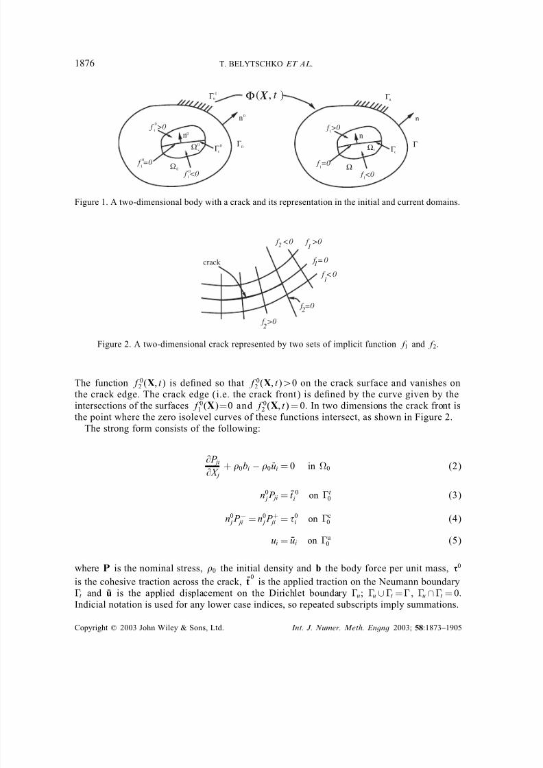
2. GOVERNING EQUATIONS AND MOTION
Consider a body 0 in the reference conÿguration as shown in Figure 1. The material co-ordinates are denoted by X and the motion is described by x= (X; t ) where x are the spatialco-ordinates. In the current conÿguration the image of 0 is . We deÿne a crack surfaceimplicitly by f1(x) = 0. To specify the edge of the crack we construct another set of implicitfunctions f2(x) whose gradient is orthogonal to the gradient of f1(x). The crack edge is given
by f1(x) = f2(x) = 0 ; fi(x) is only deÿned in a subdomain about the crack denoted by c. Wealso deÿne f0
1 (X) and f02 (X; t ) where f0
i (X) is the image of fi(x) in the initial conÿguration.The surface f0
1 (X) = 0 corresponds to the surface where hyperbolicity has been lost, i.e.the crack surface, and is also denoted by 0
c . We arbitrarily choose one side of the crack to be the direction of the normal to the crack, n0 and choose the sign of f0
1 so that
n0 ·∇Xf01¿0 (1)
Copyright ? 2003 John Wiley & Sons, Ltd. Int. J. Numer. Meth. Engng 2003; 58:1873–1905
7/30/2019 Dynamic CDynamic crack propagation based on loss of hyperbolicity and a new discontimuous enrichmentrack Pr…
http://slidepdf.com/reader/full/dynamic-cdynamic-crack-propagation-based-on-loss-of-hyperbolicity-and-a-new 4/33
1876 T. BELYTSCHKO ET AL.
ccΓ
Ω c cΓ
( , ) X t Φ
Ω
u
Γ
n
Γ
f =0
f >0
n1
1
1
Ω f <0
Γ 0
n0
f =0
f >0
f <0
n0
1
1
1
Ω
0
0
00
0
Γ u0
0
Figure 1. A two-dimensional body with a crack and its representation in the initial and current domains.
f =02
f <02
f >02
f >0
f <0
1
1
1 f =0crack
Figure 2. A two-dimensional crack represented by two sets of implicit function f1 and f2.
The function f02 (X; t ) is deÿned so that f0
2 (X; t )¿0 on the crack surface and vanishes onthe crack edge. The crack edge (i.e. the crack front) is deÿned by the curve given by the
intersections of the surfaces f01 (X)=0 and f02 (X; t ) = 0. In two dimensions the crack front isthe point where the zero isolevel curves of these functions intersect, as shown in Figure 2.
The strong form consists of the following:
@P ji
@X j+ 0bi − 0 ui = 0 in 0 (2)
n0 j P ji = t 0
i on t 0 (3)
n0 j P − ji = n0
j P + ji = 0i on c
0 (4)
ui = ui on u0 (5)
where P is the nominal stress, 0 the initial density and b the body force per unit mass, B0
is the cohesive traction across the crack, t0
is the applied traction on the Neumann boundaryt and u is the applied displacement on the Dirichlet boundary u; u ∪t = , u ∩t = 0.Indicial notation is used for any lower case indices, so repeated subscripts imply summations.
Copyright ? 2003 John Wiley & Sons, Ltd. Int. J. Numer. Meth. Engng 2003; 58:1873–1905
7/30/2019 Dynamic CDynamic crack propagation based on loss of hyperbolicity and a new discontimuous enrichmentrack Pr…
http://slidepdf.com/reader/full/dynamic-cdynamic-crack-propagation-based-on-loss-of-hyperbolicity-and-a-new 5/33
DYNAMIC CRACK PROPAGATION BASED ON LOSS OF HYPERBOLICITY 1877
We can also write the momentum equation and the traction boundary condition in terms of the Cauchy stress as follows
@ij
@x j+ bi − ui = 0 in (6)
niij = t i on t (7)
n j− ji = n j+ ji = i on c (8)
ui = ui on u (9)
where t i is the prescribed traction on the current surface, and c is the image of 0c in the
current conÿguration.We consider only rate-independent materials. The Truesdell rate of the Cauchy stress can
then be related to the rate of deformation Dkl by
∇ij = C ijkl Dkl (10)
where the tangent modulus C may depend on the stress A and other state variables.We deÿne the tensor A by
Aijkl = C ijkl + il jk (11)
The momentum equation with a constitutive law given by Equation (10) is then hyperbolicwhen
nih j Aijklnk hl¿0
∀n and h
= 0 (12)
The above conditions are identical to the conditions for ellipticity of the equations of equilibrium. They can also be viewed as a condition for material stability, since the inequalityimplies the stable response of an inÿnite medium in a uniform state of stress and strain whensubjected to the perturbation u= hei!t +k n·x (see Belytschko et al. [19]). The hyperbolicityconditions are equivalent to the requirement that the material admit a plane progressive wave(see Marsden and Hughes [20]). It also implies that the momentum equation is a hyperbolic
partial dierential equation.Extrapolating from the results of Bazant and Belytschko [1], it can be inferred that when
the hyperbolicity condition is violated for a rate-independent material, then the strain localizesto a set of measure zero on which the strain becomes inÿnite. It must be stressed that these areempirical inferences and that little appears to be known about the morphology and evolution
of such surfaces in multi-dimensions. For example, it is possible that loss of hyperbolicity ina body in R3 occurs on lines, on arrays of points, fractals, etc. However, we will assume thathyperbolicity is lost on a smooth surface.
Let the displacement ÿeld be decomposed into a continuous part and a discontinuous part,as in Armero and Garikipati [21] and Oliver [22].
u= ucont + udisc (13)
Copyright ? 2003 John Wiley & Sons, Ltd. Int. J. Numer. Meth. Engng 2003; 58:1873–1905
7/30/2019 Dynamic CDynamic crack propagation based on loss of hyperbolicity and a new discontimuous enrichmentrack Pr…
http://slidepdf.com/reader/full/dynamic-cdynamic-crack-propagation-based-on-loss-of-hyperbolicity-and-a-new 6/33
1878 T. BELYTSCHKO ET AL.
The discontinuous part of the displacement ÿeld is then given by
udisc =(t;X) H (f01 (X)) H (f0
2 (X; t )) (14)
where H is the Heaviside function given by
H ( x) =
1 x¿0
0 x¡0(15)
and (X; t ) is a continuous function that satisÿes the following conditions:
1. That vanish on the zero isolevel of f02 (X; t ), i.e.
(t;X) = 0 for Xf02 (X; t ) = 0 (16)
2. That be non-negative on the zero isolevel of f01 (X; t ), i.e.
(t;X)¿0 for X
f0
1 (X; t ) = 0 (17)
The ÿrst condition enforces continuity of the crack opening displacement at the cracktip. Thesecond condition precludes overlap of the crack surfaces.
The function f01 (X) is not a function of time. This construction of f0
1 is motivated by thefact that once hyperbolicity is lost on a surface, we can never revert to a continuum treatmenton that surface and therefore the surface must be ÿxed in the reference conÿguration. In other words, once a crack developes, the image of that crack in the reference domain is ÿxed, i.e.any crack surface that has developed is frozen. In the computational method, this implies thatthe crack surface must be considered separately from the continuum for the remainder of theanalysis. The function f0
2 (X; t ) is a function of time to reect the growth of the crack surface.The discontinuous part of deformation gradient F is obtained from its deÿnition
F discij =
@udisci
@X j=
@i
@X j H (f0
1 ) H (f02 ) + i(f0
1 )@f0
1
@X j H (f0
2 ) + i H (f01 )(f0
2 )@f0
2
@X j(18)
where (·) is the Dirac delta function. We note that
n0i =
@f01
@X i(19)
since (X; t ) = 0 at the crack edge, the last term vanishes. Therefore, the deformation gradientis given by
F discij =
@i
@X j H (f0
1 ) H (f02 ) + m0
j i(f01 ) H (f0
2 ) (20)
Thus the deformation gradient is inÿnite on the surface of lost hyperbolicity.To treat the mechanics on this surface, we then switch from a continuum description of the
constitutive behaviour Equation (10) to jump relations. We write these relations in rate formin terms of the tractions on the current surface of discontinuity:
∇i = Dij<u j= for f01 = 0; f0
2¿0 (21)
Copyright ? 2003 John Wiley & Sons, Ltd. Int. J. Numer. Meth. Engng 2003; 58:1873–1905
7/30/2019 Dynamic CDynamic crack propagation based on loss of hyperbolicity and a new discontimuous enrichmentrack Pr…
http://slidepdf.com/reader/full/dynamic-cdynamic-crack-propagation-based-on-loss-of-hyperbolicity-and-a-new 7/33
DYNAMIC CRACK PROPAGATION BASED ON LOSS OF HYPERBOLICITY 1879
where Dij is a constitutive matrix for the interface and ∇i is an objective rate of the traction(see Reference [19, p. 585]). In the numerical examples in this paper, we neglect the tangentialcomponents of the traction, i.e. only the normal component is considered.
3. FINITE ELEMENT APPROXIMATION
In this section, we describe the enriched ÿnite element approximation that models the discon-tinuity across the crack interface. Two types of models are considered:
1. Element-by-element progression where the crack progresses one complete element at atime, i.e. whenever it grows, it advances to an edge of an adjacent element.
2. Continuous progression where the crack can grow continuously within an element butonly in a ÿxed direction; the crack change its direction as it enters a new element.
In element-by-element progression, the displacement approximation is
uh(X) =n
I =1
N I (X)u I +
I ∈S N I (X) I (X)q I (22)
where q I are enrichment variables and I is given as
I (X) = H (f(X)) − H (f(X I )) (23)
where f(X)≡f01 (X) = 0 deÿnes the crack interface as shown in Figures 1 and 2 (we drop
the subscript and superscript on f), S is the set of enriched nodes, and n is the total number of nodes.
We will also use the following compact expression for the displacement:
uh(X) = n I =1
N I (X)u I +
I ∈S I (X)q I (24)
where
I (X) = N I (X) I (X) (25)
We next describe the procedure for selecting the set of nodes S to be enriched for a meshof constant strain triangular elements. The procedure depends on whether we are modellingthe nucleation of a discontinuity, say from loss of hyperbolicity in an element not contiguousto an existing crack, or the propagation of a discontinuity. We assume here that we havea constitutive relation that models both crack nucleation and crack propagation by loss of
hyperbolicity.We ÿrst describe the method for the case when the crack grows one element at a time;
consider a mesh of three-node, constant strain triangular elements. The nodes to be enrichedare selected as follows. Let the nodes of a generic element e1 be I , J , K . Let the normalto side JK be denoted n I ; it is the normal to the side opposite to node I . Suppose that thematerial in element e1 loses hyperbolicity according to Equation (12) with a normal n andelement e1 is not contiguous to any existing cracked elements. The speciÿc node I to be
Copyright ? 2003 John Wiley & Sons, Ltd. Int. J. Numer. Meth. Engng 2003; 58:1873–1905
7/30/2019 Dynamic CDynamic crack propagation based on loss of hyperbolicity and a new discontimuous enrichmentrack Pr…
http://slidepdf.com/reader/full/dynamic-cdynamic-crack-propagation-based-on-loss-of-hyperbolicity-and-a-new 8/33
1880 T. BELYTSCHKO ET AL.
(a)
(b) (c)
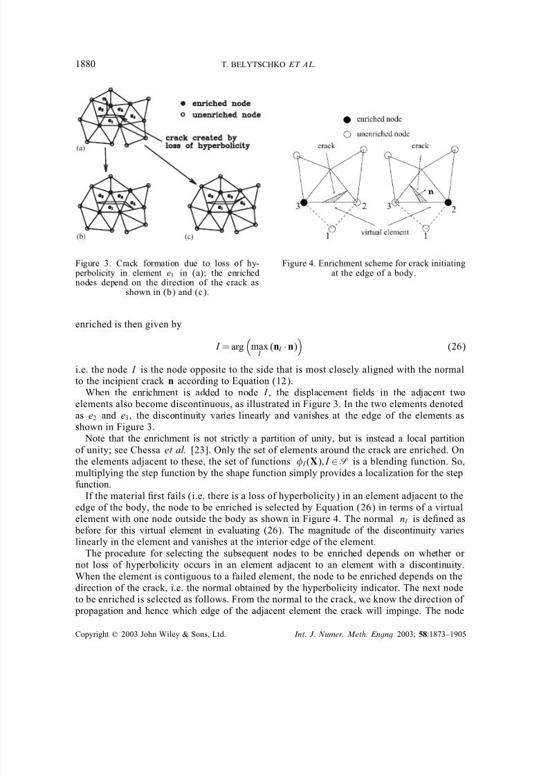
Figure 3. Crack formation due to loss of hy-
perbolicity in element e1 in (a); the enrichednodes depend on the direction of the crack as
shown in (b) and (c).
Figure 4. Enrichment scheme for crack initiating
at the edge of a body.
enriched is then given by
I = arg
max I
(n I · n)
(26)
i.e. the node I is the node opposite to the side that is most closely aligned with the normalto the incipient crack n according to Equation (12).
When the enrichment is added to node I , the displacement ÿelds in the adjacent two
elements also become discontinuous, as illustrated in Figure 3. In the two elements denotedas e2 and e3, the discontinuity varies linearly and vanishes at the edge of the elements asshown in Figure 3.
Note that the enrichment is not strictly a partition of unity, but is instead a local partitionof unity; see Chessa et al. [23]. Only the set of elements around the crack are enriched. Onthe elements adjacent to these, the set of functions I (X); I ∈S is a blending function. So,multiplying the step function by the shape function simply provides a localization for the stepfunction.
If the material ÿrst fails (i.e. there is a loss of hyperbolicity) in an element adjacent to theedge of the body, the node to be enriched is selected by Equation (26) in terms of a virtualelement with one node outside the body as shown in Figure 4. The normal n I is deÿned as
before for this virtual element in evaluating (26). The magnitude of the discontinuity varies
linearly in the element and vanishes at the interior edge of the element.The procedure for selecting the subsequent nodes to be enriched depends on whether or
not loss of hyperbolicity occurs in an element adjacent to an element with a discontinuity.When the element is contiguous to a failed element, the node to be enriched depends on thedirection of the crack, i.e. the normal obtained by the hyperbolicity indicator. The next nodeto be enriched is selected as follows. From the normal to the crack, we know the direction of
propagation and hence which edge of the adjacent element the crack will impinge. The node
Copyright ? 2003 John Wiley & Sons, Ltd. Int. J. Numer. Meth. Engng 2003; 58:1873–1905
7/30/2019 Dynamic CDynamic crack propagation based on loss of hyperbolicity and a new discontimuous enrichmentrack Pr…
http://slidepdf.com/reader/full/dynamic-cdynamic-crack-propagation-based-on-loss-of-hyperbolicity-and-a-new 9/33
DYNAMIC CRACK PROPAGATION BASED ON LOSS OF HYPERBOLICITY 1881
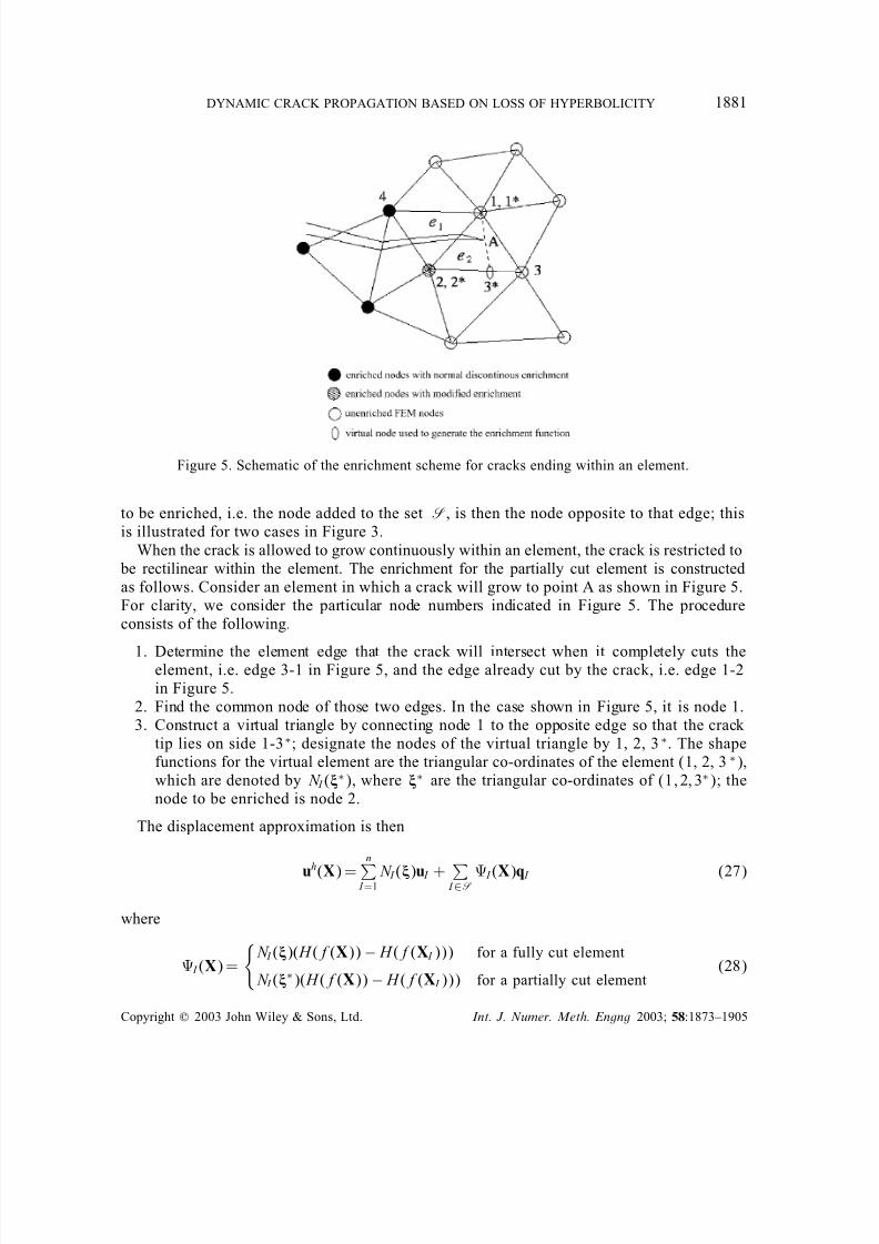
Figure 5. Schematic of the enrichment scheme for cracks ending within an element.
to be enriched, i.e. the node added to the set S, is then the node opposite to that edge; thisis illustrated for two cases in Figure 3.
When the crack is allowed to grow continuously within an element, the crack is restricted to be rectilinear within the element. The enrichment for the partially cut element is constructedas follows. Consider an element in which a crack will grow to point A as shown in Figure 5.For clarity, we consider the particular node numbers indicated in Figure 5. The procedureconsists of the following.
1. Determine the element edge that the crack will intersect when it completely cuts theelement, i.e. edge 3-1 in Figure 5, and the edge already cut by the crack, i.e. edge 1-2in Figure 5.
2. Find the common node of those two edges. In the case shown in Figure 5, it is node 1.3. Construct a virtual triangle by connecting node 1 to the opposite edge so that the crack
tip lies on side 1-3∗; designate the nodes of the virtual triangle by 1, 2, 3∗. The shapefunctions for the virtual element are the triangular co-ordinates of the element (1, 2, 3∗),which are denoted by N I (^
∗), where ^∗ are the triangular co-ordinates of (1; 2; 3∗); thenode to be enriched is node 2.
The displacement approximation is then
uh(X) =
n I =1
N I (^)u I +
I ∈S I (X)q I (27)
where
I (X) =
N I (^)( H (f(X))− H (f(X I ))) for a fully cut element
N I (^∗)( H (f(X)) − H (f(X I ))) for a partially cut element
(28)
Copyright ? 2003 John Wiley & Sons, Ltd. Int. J. Numer. Meth. Engng 2003; 58:1873–1905
7/30/2019 Dynamic CDynamic crack propagation based on loss of hyperbolicity and a new discontimuous enrichmentrack Pr…
http://slidepdf.com/reader/full/dynamic-cdynamic-crack-propagation-based-on-loss-of-hyperbolicity-and-a-new 10/33
1882 T. BELYTSCHKO ET AL.
We next show that this displacement approximation is continuous across edge 1-2. Thedisplacement along edge 1-2 in element e1 in Figure 5 is
uh
(X) = N 1u1 + N 2u2 + N 4u4 + N 22q2 + N 44q4
= N 1u1 + N 2u2 + N 22q2 (29)
The displacement along edge 1-2 in element e2 is
uh(X) = N 1u1 + N 2u2 + N 3u3 + N ∗2 2q2
= N 1u1 + N 2u2 + N ∗2 2q2 (30)
where N ∗ I = N I (∗ I ). The last step in the above two equations use the condition that N 4 and N 3 vanish along edge 1-2. Since the modiÿed shape function N ∗2 is equivalent to the standardshape function N 2 on edge 1-2, i.e. N 2(^∗) = N 2(^), the displacement ÿeld is continuous acrossedge 1-2. The partially enriched element developed here for linear triangular elements has beenextended to quadratic triangular elements by Zi and Belytschko [24].
4. COHESIVE LAW
The mechanics of the discontinuity that is created by loss of hyperbolicity, i.e. the crack,will be treated by a cohesive model. In a cohesive model, the energy dissipated due to crack
propagation is modelled by a traction–displacement jump relationship at the crack surface; seeBarenblatt [25], Dugdale [26], Hillerborg et al. [27], Planas and Elices [28], etc.
We only consider cohesive laws involving the normal component of the traction. Thedisplacement jump N is deÿned by
N = n · <u= = n · I ∈S
N I (X)q I (31)
The last term in the above is derived as follows from (27):
<u= = u(X+)− u(X−)
=n
I =1
N I (X+)u I +
I ∈S
N I (X+) I (X
+)q I
− n I =1
N I (X−)u I −
I ∈S
N I (X−) I (X
−)q I
=
I ∈S
N I (X)( I (X+) − I (X
−))q I
=
I ∈S
N I (X)q I (32)
Copyright ? 2003 John Wiley & Sons, Ltd. Int. J. Numer. Meth. Engng 2003; 58:1873–1905
7/30/2019 Dynamic CDynamic crack propagation based on loss of hyperbolicity and a new discontimuous enrichmentrack Pr…
http://slidepdf.com/reader/full/dynamic-cdynamic-crack-propagation-based-on-loss-of-hyperbolicity-and-a-new 11/33
DYNAMIC CRACK PROPAGATION BASED ON LOSS OF HYPERBOLICITY 1883
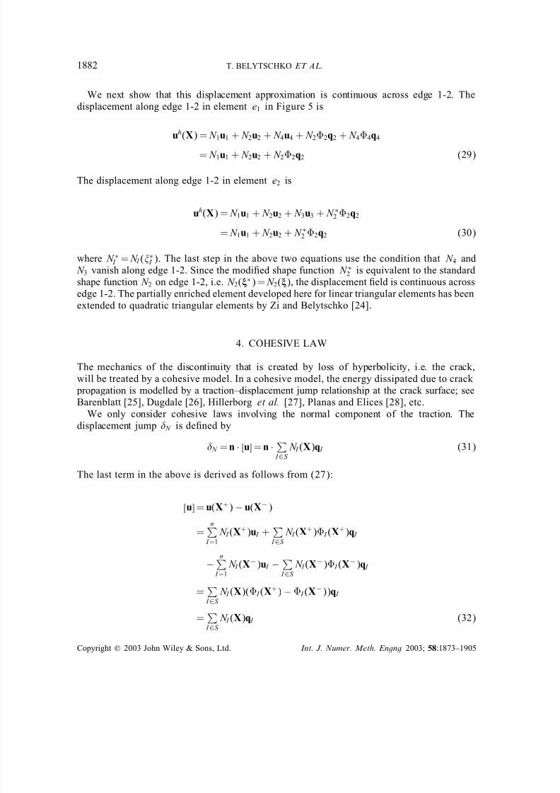
Figure 6. Two dierent cohesive models, in which the area under a cohesive law is the fracture energyG F: (a) linear cohesive law; and (b) bilinear cohesive law.
In the above, X± represents X ± n0 where → 0 and n0 is the normal to the crack surfacein the reference conÿguration. In the second line of the above, we have used the continuityof the shape functions across the crack, i.e. that N I (X
+) = N I (X−).
The normal traction is deÿned by
N =n · B (33)
We will use traction laws of the form depicted in Figure 6 with a radial return algorithm asin References [5, 29, 30]. When the material switches from continuous to discontinuous thetraction at the interface takes on the current value of the traction in the element. The cohesivestrength max is not a ÿxed parameter of the cohesive law. Otherwise, the tractions can besuciently discontinuous to lead to noise (see Papoulia et al. [31]).
Given the shape of a cohesive law, the cohesive crack model is completely deÿned by thefracture energy G F and the cohesive strength max. Therefore, the critical crack opening max
is calculated from G F and max. For example, for the linear cohesive model shown in Figure6(a), the critical crack opening max is
max = 2G Fmax
(34)
The traction law for the case shown in Figure 6(a) is formulated as an incremental lawwith radial return by the following algorithm
if n+1 N 60 go to end
trial N = n
N + E n(n+1 N − n
N )
if trial N ¡f(n+1
N ) go to end
n+1 N = f(n+1)
E
n+1
=
n+1
N =
n+1
N
end
Note that if n+1 N 60, i.e. whenever the crack surfaces close, the tractions N are computed by
the equations of motion; the cohesive law is only active when the crack surfaces are separated.The relation between traction and the jump in displacement does not suce to provide
closure to the problem. In other words, the cohesive law and the strong form given by
Copyright ? 2003 John Wiley & Sons, Ltd. Int. J. Numer. Meth. Engng 2003; 58:1873–1905
7/30/2019 Dynamic CDynamic crack propagation based on loss of hyperbolicity and a new discontimuous enrichmentrack Pr…
http://slidepdf.com/reader/full/dynamic-cdynamic-crack-propagation-based-on-loss-of-hyperbolicity-and-a-new 12/33
1884 T. BELYTSCHKO ET AL.
y θφ
n
h
x
Figure 7. n and h in two dimensions. Figure 8. Crack increment and the hyperbolicityindicator e.
Equations (7)–(10) do not provide a complete statement of the problem of crack propagation.Closure is provided by the loss of hyperbolicity condition, which can be viewed as a crack
propagation law. Similarly, a maximum tensile stress criterion can provide closure.
It is interesting to observe that in the inter-element approach of References [3, 5], a crack propagation law is not needed. Since the crack advances one edge at a time (or has the possibility of advancing partially through all edges when the cohesive model joins all elementas in Xu and Needleman [3]), there is no need for a propagation law. Thus the inter-elementapproach achieves closure by the discretization.
The following describes our methodology for using the loss of hyperbolicity criterion to propagate the crack. The methodology described here is only applicable to rate-independentmaterials. This method also allows a new crack to initiate and determines its direction. Thusthere is no need for a crack growth law: the crack growth, i.e. the cracktip velocity and thedirection of the crack, are determined by the constitutive equation.
In essence, the method uses the polarization of the plane wave emanating from the hyper- bolicity condition to set the direction of the crack and the value of the hyperbolicity condition
to set the speed. Let
e = minn; h
(nih j Aijklnk hl) (35)
where A is deÿned in (11). We call e the hyperbolicity indicator. The momentum equationsremain hyperbolic as long as e¿0. If the inequality e¿0 is violated in the neighborhoodof a cracktip, we then choose the normal of the surface increment (line increment in twodimensions) to be the vector n that minimizes e. The direction of the cracktip is denoted bya unit vector s, and it is given by
s · n= 0 (36)
For example, in two dimensions, we can express n and h by two angles  and , i.e.
n1 = cos Â, n2 = sin Â, h1 = cos , h2 = sin ; see Figure 7. The hyperbolicity indicator cor-responds to the minimum of the right hand side of (35), so
@e
@Â= 0 (37)
@e
@= 0 (38)
Copyright ? 2003 John Wiley & Sons, Ltd. Int. J. Numer. Meth. Engng 2003; 58:1873–1905
7/30/2019 Dynamic CDynamic crack propagation based on loss of hyperbolicity and a new discontimuous enrichmentrack Pr…
http://slidepdf.com/reader/full/dynamic-cdynamic-crack-propagation-based-on-loss-of-hyperbolicity-and-a-new 13/33
DYNAMIC CRACK PROPAGATION BASED ON LOSS OF HYPERBOLICITY 1885
Substituting Equation (35) into the above equations, we get two equations for  and :
dni
dÂh j Aijklnk hl + nih j Aijkl
dnk
dÂhl = 0 (39)
nidh j
dAijklnk hl + nih j Aijklnk
dhl
d= 0 (40)
For the material laws we have used, n and h are approximately parallel to each other. Thismeans that the incipient instability is associated with a displacement normal to the surface,which corresponds to crack opening.
The hyperbolicity indicator is a piecewise continuous function, i.e. a C −1 function, since itdepends on the tangent modulus and the stresses, which are C −1. This prevents the smoothmotion of the cracktip in an element. Therefore, we project e onto a C 0 ÿeld. The continuousvalues of the hyperbolicity indicator around the crack tip are obtained by a least-square ÿt to
the piecewise continuous indicator values (e.g. see Reference [7]). Let e = N I (X)e I ∈C 0, andeh ∈C −1 be a piecewise continuous ÿeld. The least-square ÿt for the hyperbolicity indicator is obtained by projecting the piecewise continuous ÿeld onto a C 0 ÿeld. This is done by min-imizing the square of the dierence between the C 0 projection e = I N I e I and the piecewisecontinuous data eh obtained from the solution:
min1
2
(eh − e)2 d (41)
To ÿnd the minimum of the above, we set its derivative with respect to the e J to zero:
@
2@e J
(eh
−e)2 d = 0 (42)
From above we can obtain the equation for e I :
(eh N J − e I N I N J ) d = 0 (43)
The least-square ÿt is only applied to several elements surrounding the crack tip, because its purpose is to obtain the direction and velocity of the crack tip. From experience, a subdomainwith a radius of 3 to 4 elements is enough.
Since the hyperbolicity indicator should always vanish at the crack tip, it follows that atthe crack tip.
@e
@t + vc
i e; i = 0 (44)
where vci is the velocity of the crack tip. The cracktip velocity can be expressed as
vci = vc si (45)
Copyright ? 2003 John Wiley & Sons, Ltd. Int. J. Numer. Meth. Engng 2003; 58:1873–1905
7/30/2019 Dynamic CDynamic crack propagation based on loss of hyperbolicity and a new discontimuous enrichmentrack Pr…
http://slidepdf.com/reader/full/dynamic-cdynamic-crack-propagation-based-on-loss-of-hyperbolicity-and-a-new 14/33
1886 T. BELYTSCHKO ET AL.
where vc is the crack speed and s is deÿned in (36). Substituting this deÿnition into (44)gives
@e
@t + vc s
ie
; i= 0 (46)
from which we obtain
vc =−( sie; i)−1 @e
@t =−(s · e)−1 @e
@t (47)
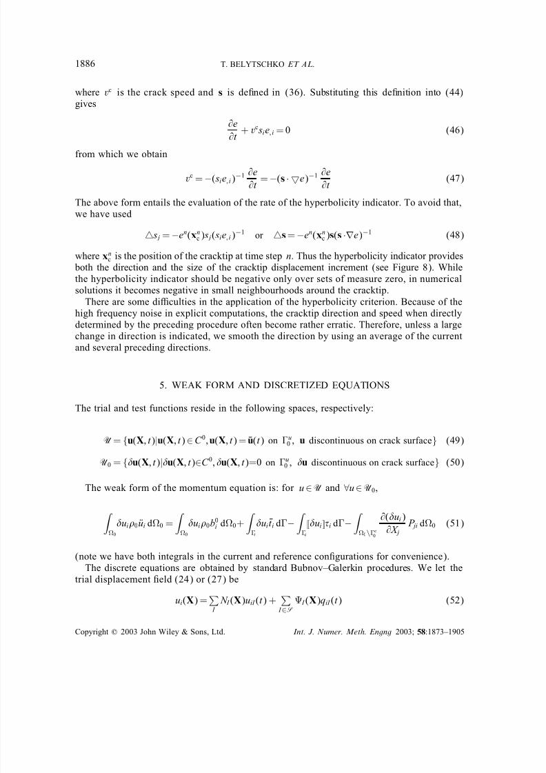
The above form entails the evaluation of the rate of the hyperbolicity indicator. To avoid that,we have used
s j =−en(xnc ) s j( sie; i)
−1 or s=−en(xnc )s(s ·∇e)−1 (48)
where xnc is the position of the cracktip at time step n. Thus the hyperbolicity indicator provides
both the direction and the size of the cracktip displacement increment (see Figure 8). Whilethe hyperbolicity indicator should be negative only over sets of measure zero, in numericalsolutions it becomes negative in small neighbourhoods around the cracktip.
There are some diculties in the application of the hyperbolicity criterion. Because of thehigh frequency noise in explicit computations, the cracktip direction and speed when directlydetermined by the preceding procedure often become rather erratic. Therefore, unless a largechange in direction is indicated, we smooth the direction by using an average of the currentand several preceding directions.
5. WEAK FORM AND DISCRETIZED EQUATIONS
The trial and test functions reside in the following spaces, respectively:
U= u(X; t )|u(X; t )∈C 0;u(X; t ) = u(t ) on u0 ; u discontinuous on crack surface (49)
U0 = u(X; t )|u(X; t )∈C 0; u(X; t )=0 on u0 ; u discontinuous on crack surface (50)
The weak form of the momentum equation is: for u∈U and ∀u∈U0,
0
ui0 ui d0 =
0
ui0b0i d0+
t
ui t i d−
c
<ui=i d−
0\c0
@(ui)
@X j P ji d0 (51)
(note we have both integrals in the current and reference conÿgurations for convenience).The discrete equations are obtained by standard Bubnov–Galerkin procedures. We let the
trial displacement ÿeld (24) or (27) be
ui(X) = I
N I (X)uiI (t ) +
I ∈S
I (X)qiI (t ) (52)
Copyright ? 2003 John Wiley & Sons, Ltd. Int. J. Numer. Meth. Engng 2003; 58:1873–1905
7/30/2019 Dynamic CDynamic crack propagation based on loss of hyperbolicity and a new discontimuous enrichmentrack Pr…
http://slidepdf.com/reader/full/dynamic-cdynamic-crack-propagation-based-on-loss-of-hyperbolicity-and-a-new 15/33
DYNAMIC CRACK PROPAGATION BASED ON LOSS OF HYPERBOLICITY 1887
where I (X) have been deÿned in Equations (25) and (28). The test displacement ÿeld is
ui(X) =
I
uiI (t ) N I (X) +
I ∈SqiI (t ) I (X) (53)
In taking any derivatives, we consider 0 the open set with 0c excluded. Furthermore, we
carefully distinguish between +c and −c in evaluating the surface integrals of the crack. The
derivatives of the trial displacement ÿeld are then given by
@ui
@X j= I
N I; juiI +
I ∈S I; jqiI (54)
A similar expression holds for the derivatives of the test displacement ÿeld @ui=@X j.Substituting the above into the weak form Equation (51) gives
I
[uiI (fintiI + M u IJ uiJ + M
uq IJ qiJ
−fext
iI ) + qiI (QintiI + M
q IJ qiJ + M
uq JI uiJ
−Qext
iI )] = 0 (55)
for all uiI and qiI that are not constrained by displacement boundary conditions or theinequality (17); the two parentheses give the discrete equations. In the above,
fintiI =
0\c
0
@N I
@X j P ji d0
fextiI =
t
0
N I t 0
i d0 +
0
N I 0bi d0 (56)
QintiI =
0\c0
@ I @X j
P ji d0
QextiI =
t
0
I t 0i d0 +
0
I 0bi d0 −
c
N I i d (57)
M u IJ =
0
N I N J d0
M uq IJ =
0
N I J d0
M q IJ =
0
I J d0 (58)
Note that the cohesive traction only eects the nodal force QextiI , and that it is evaluated
in the current conÿguration. As noted in Reference [19], the nodal forces can be evaluatedin either the current or the reference conÿgurations; it is often convenient to evaluate surfaceintegrals over the current conÿguration, volume integrals over the initial conÿguration.
Copyright ? 2003 John Wiley & Sons, Ltd. Int. J. Numer. Meth. Engng 2003; 58:1873–1905
7/30/2019 Dynamic CDynamic crack propagation based on loss of hyperbolicity and a new discontimuous enrichmentrack Pr…
http://slidepdf.com/reader/full/dynamic-cdynamic-crack-propagation-based-on-loss-of-hyperbolicity-and-a-new 16/33
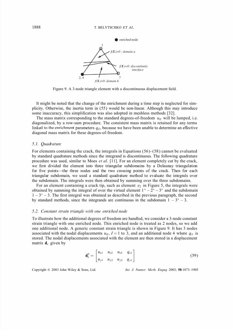
1888 T. BELYTSCHKO ET AL.
2, 4
f( )=0: discontinuity
3
1
interface
f( )>0 : domain a
enriched node
f( )<0: domain b
X
X
X
Figure 9. A 3-node triangle element with a discontinuous displacement ÿeld.
It might be noted that the change of the enrichment during a time step is neglected for sim- plicity. Otherwise, the inertia term in (55) would be non-linear. Although this may introducesome inaccuracy, this simpliÿcation was also adopted in meshless methods [32].
The mass matrix corresponding to the standard degrees-of-freedom uiI will be lumped, i.e.diagonalized, by a row-sum procedure. The consistent mass matrix is retained for any termslinked to the enrichment parameters qiI , because we have been unable to determine an eectivediagonal mass matrix for these degrees-of-freedom.
5.1. Quadrature
For elements containing the crack, the integrals in Equations (56)–(58) cannot be evaluated by standard quadrature methods since the integrand is discontinuous. The following quadrature procedure was used, similar to Moes et al. [11]. For an element completely cut by the crack,we ÿrst divided the element into three triangular subdomains by a Delaunay triangulationfor ÿve points—the three nodes and the two crossing points of the crack. Then for eachtriangular subdomain, we used a standard quadrature method to evaluate the integrals over the subdomain. The integrals were then obtained by summing over the three subdomains.
For an element containing a crack tip, such as element e2 in Figure 5, the integrals wereobtained by summing the integral of over the virtual element 1∗− 2∗−3∗ and the subdomain1− 3∗− 3. The ÿrst integral was obtained as described in the previous paragraph, the second
by standard methods, since the integrands are continuous in the subdomain 1 − 3∗ − 3.
5.2. Constant strain triangle with one enriched node
To illustrate how the additional degrees of freedom are handled, we consider a 3-node constantstrain triangle with one enriched node. This enriched node is treated as 2 nodes, so we addone additional node. A generic constant strain triangle is shown in Figure 9. It has 3 nodesassociated with the nodal displacements uiI , I = 1 to 3, and an additional node 4 where qi1 isstored. The nodal displacements associated with the element are then stored in a displacementmatrix de given by
dTe =
u x1 u x2 u x3 q x1
uy1 uy2 uy3 qy1
(59)
Copyright ? 2003 John Wiley & Sons, Ltd. Int. J. Numer. Meth. Engng 2003; 58:1873–1905
7/30/2019 Dynamic CDynamic crack propagation based on loss of hyperbolicity and a new discontimuous enrichmentrack Pr…
http://slidepdf.com/reader/full/dynamic-cdynamic-crack-propagation-based-on-loss-of-hyperbolicity-and-a-new 17/33
DYNAMIC CRACK PROPAGATION BASED ON LOSS OF HYPERBOLICITY 1889
The corresponding nodal internal forces are
f inte T
= f x1 f x2 f x3 Q x1
fy1 fy2 fy3 Qy1 (60)
with a similar expression for the external nodal forces.The displacement ÿeld is
u x
uy
=
u x1 u x2 u x3 q x1
uy1 uy2 uy3 qy1
N 1
N 2
N 3
1
≡dT
e N (61)
The displacement gradient is
@u x
@X
@u x
@Y
@uy
@X
@uy
@Y
=
u x1 u x2 u x3 q x1
uy1 uy2 uy3 qy1
N 1; X N 1; Y
N 2; X N 2; Y
N 3; X N 3; Y
N 1; X 1 N 1; Y 1
(62)
Note that we do not include the terms N 11; X = N 1(f(x))f; X or N 11; Y = N 1(f(x))f; Y ,since the continuum is restricted to the open set 0\c
0 .The internal nodal forces are given by
f inte =
f x1 fy1
f x2 fy2
f x3 fy3
Q x1 Qy1
int
=
0\c
0
N 1; X N 1; Y
N 2; X N 2; Y
N 3; X N 3; Y
N 1; X 1 N 1; Y 1
P 11 P 12
P 21 P 22
d0 (63)
The cohesive tractions are treated as external nodal forces that are given later. For an elementcompletely cut by a crack the stress is piecewise constant and will be denoted by P aij and P bij
for subdomain a and b, respectively. We denote the areas of the two subdomain by Aa0 and
Ab0. The nodal forces are then given by
f inte =
Aa0
2 A0
Y 23 X 32
Y 31 X 13
Y 12 X 21
0 0
P a11 P a12
P a21 P a22
+
Ab0
2 A0
Y 23 X 32
Y 31 X 13
Y 12 X 21
−2Y 23 −2 X 32
P b11 P b12
P b21 P b22
(64)
Copyright ? 2003 John Wiley & Sons, Ltd. Int. J. Numer. Meth. Engng 2003; 58:1873–1905
7/30/2019 Dynamic CDynamic crack propagation based on loss of hyperbolicity and a new discontimuous enrichmentrack Pr…
http://slidepdf.com/reader/full/dynamic-cdynamic-crack-propagation-based-on-loss-of-hyperbolicity-and-a-new 18/33
1890 T. BELYTSCHKO ET AL.
where X IJ = X I − X J , etc. This corresponding expression in terms of the updated co-ordinatesand the Cauchy stress is
f inte =
Aa
2 A
y23 x32
y31 x13
y12 x21
0 0
a11 a
12
a21 a
22
+
Ab
2 A
y23 x32
y31 x13
y12 x21
−2y23 −2 x32
b11 b
12
b21 b
22
(65)
In the absence of body forces and boundary tractions, the external nodal forces are:
f exte =
f x1 fy1
f x2 fy2
f x3 fy3
Q x1 Qy1
ext
=
c
0 0
0 0
0 0
N 1 N 1
x 0
0 y
d (66)
5.3. Implicit–explicit time integration
Explicit time integration was not used over the entire mesh because the critical time step inelements traversed by the crack can be very small. We examined the relationship betweendiscontinuity locations and critical time steps for linear one dimensional elements. We foundthat the critical time step tends to zero as the discontinuity approaches the element nodes.
So we adopt an implicit–explicit time integration scheme [33]) in our computation. For elements with enriched nodes, we use implicit integration while for elements without anyenrichment we use explicit integration. It is necessary to solve a set of non-linear equationsdue to the non-linearity of the constitutive model. Since the extension of the implicit–explicit
scheme to consider non-linearities is straightforward, the procedure is not described here.
6. NUMERICAL EXAMPLES
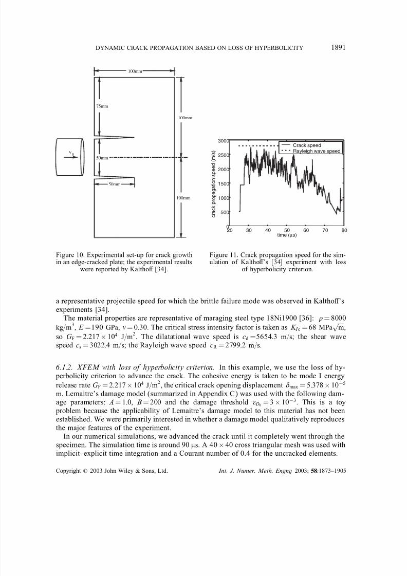
6.1. Edge-cracked plate under impulsive loading
6.1.1. Problem description In experiments of Kaltho [34], a plate with two edge notches isimpacted by a projectile as shown in Figure 10. By modifying the projectile speed and theacuity of the notch tip, two dierent failure modes were observed. At higher strain rates, ashear localization mode due to the formation of a shear band ahead of the notch at a negativeangle of about −10 was observed. On the other hand, at lower strain rates, a brittle fracture
mode with a propagation angle of ∼ 70
was observed. In this study, we focused on the brittle failure.
Twofold symmetry is used in modelling the problem. A symmetry condition was appliedon the bottom edge of the model (uy = 0), and a step velocity on the cracked edge for 06y625 mm; the other edges are traction-free. We assume that the projectile has the sameelastic impedance as the plate section that is impacted, so the impact velocity is approximatelyone-half of the projectile speed [35]. The impact velocity is chosen as v0 = 16:5 m= s, which is
Copyright ? 2003 John Wiley & Sons, Ltd. Int. J. Numer. Meth. Engng 2003; 58:1873–1905
7/30/2019 Dynamic CDynamic crack propagation based on loss of hyperbolicity and a new discontimuous enrichmentrack Pr…
http://slidepdf.com/reader/full/dynamic-cdynamic-crack-propagation-based-on-loss-of-hyperbolicity-and-a-new 19/33
DYNAMIC CRACK PROPAGATION BASED ON LOSS OF HYPERBOLICITY 1891
100mm
v0
50mm
50mm
100mm
100mm
75mm
20 30 40 50 60 70 800
500
1000
1500
2000
2500
3000
time (µs)
c r a c k p r o p a g a t i o n s p e e d ( m / s )
Crack speedRayleigh wave speed
Figure 10. Experimental set-up for crack growthin an edge-cracked plate; the experimental results
were reported by Kaltho [34].
Figure 11. Crack propagation speed for the sim-ulation of Kaltho’s [34] experiment with loss
of hyperbolicity criterion.
a representative projectile speed for which the brittle failure mode was observed in Kaltho’sexperiments [34].
The material properties are representative of maraging steel type 18Ni1900 [36]: = 8000
kg= m3, E =190 GPa, = 0:30. The critical stress intensity factor is taken as K I c = 68 MPa
√ m,
so G F = 2:217× 104 J= m2
. The dilatational wave speed is cd =5654:3 m= s; the shear wavespeed cs = 3022:4 m= s; the Rayleigh wave speed cR = 2799:2 m= s.
6.1.2. XFEM with loss of hyperbolicity criterion. In this example, we use the loss of hy- perbolicity criterion to advance the crack. The cohesive energy is taken to be mode I energy
release rate G F = 2:217× 104 J= m2
, the critical crack opening displacement max = 5:378× 10−5
m. Lemaitre’s damage model (summarized in Appendix C) was used with the following dam-
age parameters: A = 1:0, B = 200 and the damage threshold D0 = 3× 10⁻³
. This is a toy problem because the applicability of Lemaitre’s damage model to this material has not beenestablished. We were primarily interested in whether a damage model qualitatively reproducesthe major features of the experiment.
In our numerical simulations, we advanced the crack until it completely went through thespecimen. The simulation time is around 90 s. A 40× 40 cross triangular mesh was used withimplicit–explicit time integration and a Courant number of 0.4 for the uncracked elements.
Copyright ? 2003 John Wiley & Sons, Ltd. Int. J. Numer. Meth. Engng 2003; 58:1873–1905
7/30/2019 Dynamic CDynamic crack propagation based on loss of hyperbolicity and a new discontimuous enrichmentrack Pr…
http://slidepdf.com/reader/full/dynamic-cdynamic-crack-propagation-based-on-loss-of-hyperbolicity-and-a-new 20/33
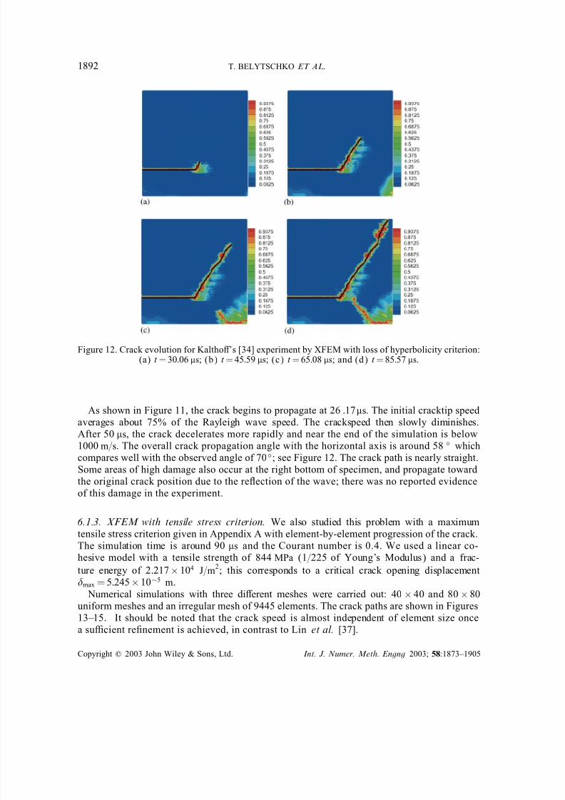
1892 T. BELYTSCHKO ET AL.
Figure 12. Crack evolution for Kaltho’s [34] experiment by XFEM with loss of hyperbolicity criterion:(a) t = 30:06 s; (b) t = 45:59 s; (c) t = 65:08 s; and (d) t = 85:57 s.
As shown in Figure 11, the crack begins to propagate at 26 :17s. The initial cracktip speed
averages about 75% of the Rayleigh wave speed. The crackspeed then slowly diminishes.After 50 s, the crack decelerates more rapidly and near the end of the simulation is below1000 m= s. The overall crack propagation angle with the horizontal axis is around 58 whichcompares well with the observed angle of 70; see Figure 12. The crack path is nearly straight.Some areas of high damage also occur at the right bottom of specimen, and propagate towardthe original crack position due to the reection of the wave; there was no reported evidenceof this damage in the experiment.
6.1.3. XFEM with tensile stress criterion. We also studied this problem with a maximumtensile stress criterion given in Appendix A with element-by-element progression of the crack.The simulation time is around 90 s and the Courant number is 0.4. We used a linear co-
hesive model with a tensile strength of 844 MPa (1= 225 of Young’s Modulus) and a frac-ture energy of 2:217× 104 J= m
2; this corresponds to a critical crack opening displacement
max = 5:245× 10−5 m. Numerical simulations with three dierent meshes were carried out: 40× 40 and 80× 80
uniform meshes and an irregular mesh of 9445 elements. The crack paths are shown in Figures13–15. It should be noted that the crack speed is almost independent of element size oncea sucient reÿnement is achieved, in contrast to Lin et al. [37].
Copyright ? 2003 John Wiley & Sons, Ltd. Int. J. Numer. Meth. Engng 2003; 58:1873–1905
7/30/2019 Dynamic CDynamic crack propagation based on loss of hyperbolicity and a new discontimuous enrichmentrack Pr…
http://slidepdf.com/reader/full/dynamic-cdynamic-crack-propagation-based-on-loss-of-hyperbolicity-and-a-new 21/33
DYNAMIC CRACK PROPAGATION BASED ON LOSS OF HYPERBOLICITY 1893
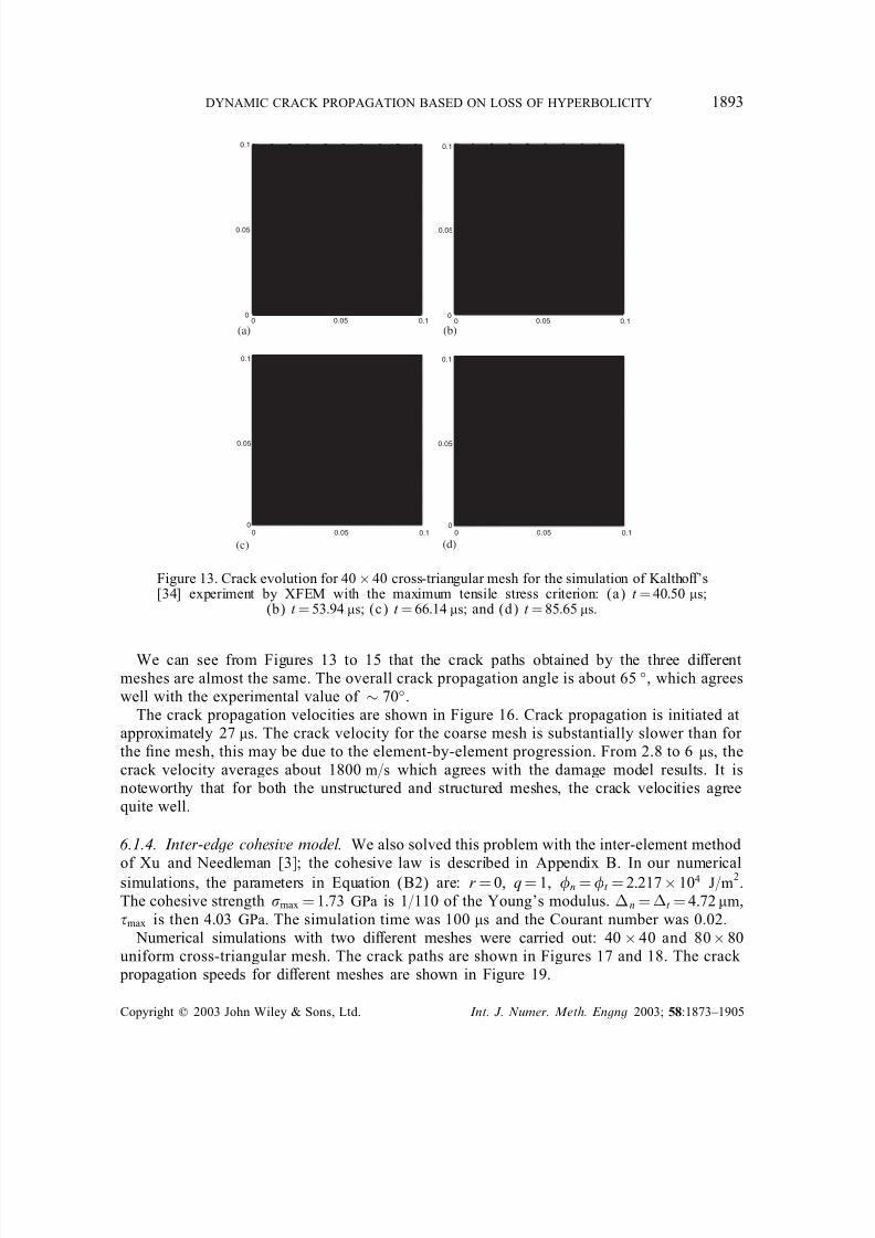
0 0.05 0.10
0.05
0.1
0
0.05
0.1
0
0.05
0.1
0
0.05
0.1
0 0.05 0.1
(b)(a)
0 0.05 0.1
(c)
0 0.05 0.1
(d)
Figure 13. Crack evolution for 40× 40 cross-triangular mesh for the simulation of Kaltho’s[34] experiment by XFEM with the maximum tensile stress criterion: (a) t = 40:50 s;
(b) t = 53:94 s; (c) t = 66:14 s; and (d) t = 85:65 s.
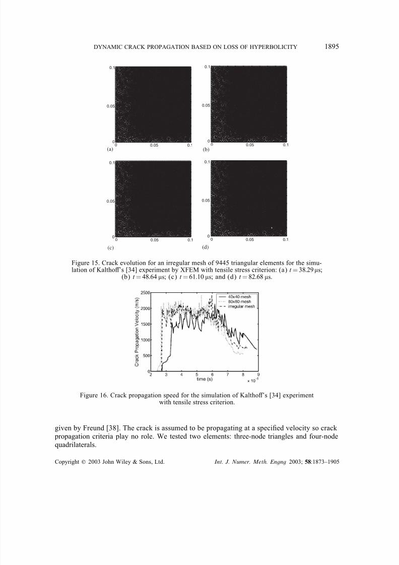
We can see from Figures 13 to 15 that the crack paths obtained by the three dierentmeshes are almost the same. The overall crack propagation angle is about 65, which agreeswell with the experimental value of ∼ 70.
The crack propagation velocities are shown in Figure 16. Crack propagation is initiated atapproximately 27 s. The crack velocity for the coarse mesh is substantially slower than for the ÿne mesh, this may be due to the element-by-element progression. From 2.8 to 6 s, thecrack velocity averages about 1800 m= s which agrees with the damage model results. It isnoteworthy that for both the unstructured and structured meshes, the crack velocities agreequite well.
6.1.4. Inter-edge cohesive model. We also solved this problem with the inter-element method
of Xu and Needleman [3]; the cohesive law is described in Appendix B. In our numericalsimulations, the parameters in Equation (B2) are: r = 0, q = 1, n = t = 2:217× 104 J= m
2.
The cohesive strength max = 1:73 GPa is 1= 110 of the Young’s modulus. n = t = 4:72 m,max is then 4:03 GPa. The simulation time was 100 s and the Courant number was 0.02.
Numerical simulations with two dierent meshes were carried out: 40× 40 and 80× 80uniform cross-triangular mesh. The crack paths are shown in Figures 17 and 18. The crack
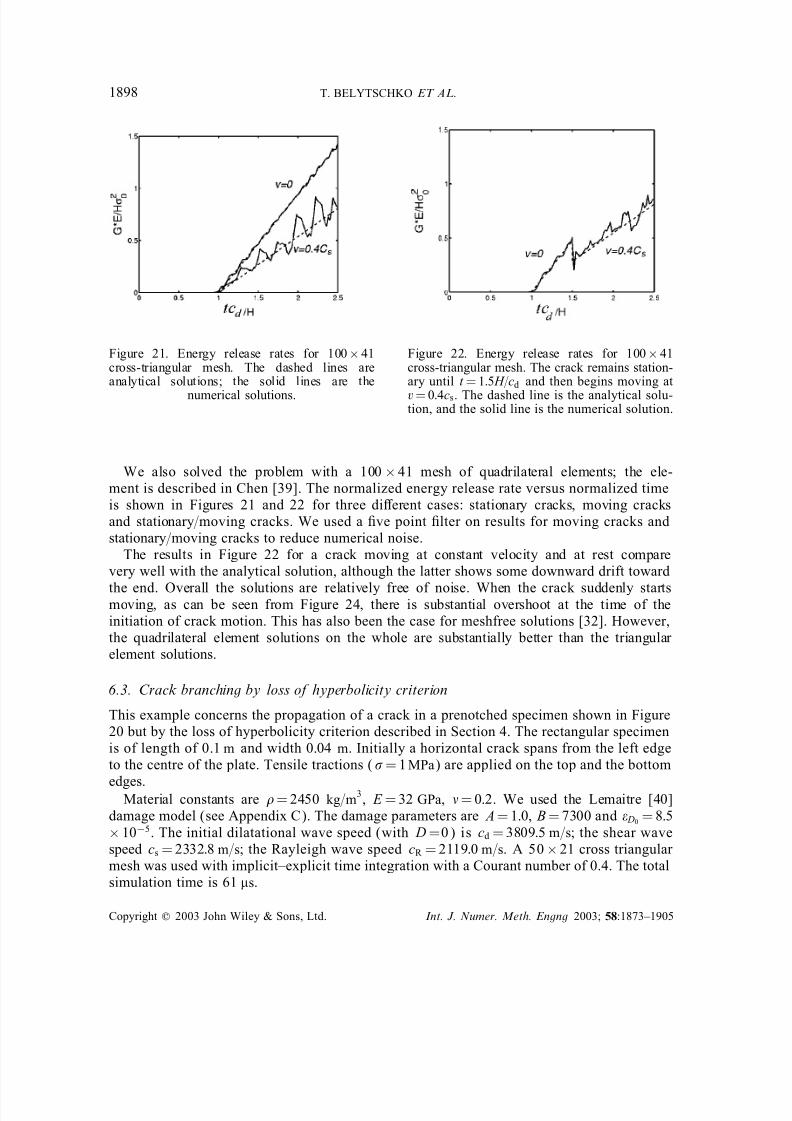
propagation speeds for dierent meshes are shown in Figure 19.
Copyright ? 2003 John Wiley & Sons, Ltd. Int. J. Numer. Meth. Engng 2003; 58:1873–1905
7/30/2019 Dynamic CDynamic crack propagation based on loss of hyperbolicity and a new discontimuous enrichmentrack Pr…
http://slidepdf.com/reader/full/dynamic-cdynamic-crack-propagation-based-on-loss-of-hyperbolicity-and-a-new 22/33
1894 T. BELYTSCHKO ET AL.
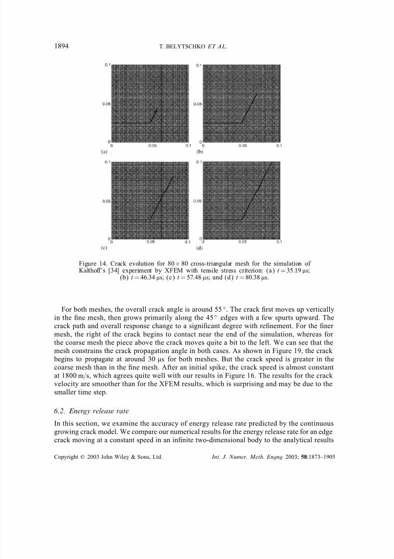
Figure 14. Crack evolution for 80× 80 cross-triangular mesh for the simulation of Kaltho’s [34] experiment by XFEM with tensile stress criterion: (a) t = 35:19 s;
(b) t = 46:34 s; (c) t = 57:48 s; and (d) t = 80:38 s.
For both meshes, the overall crack angle is around 55. The crack ÿrst moves up verticallyin the ÿne mesh, then grows primarily along the 45 edges with a few spurts upward. Thecrack path and overall response change to a signiÿcant degree with reÿnement. For the ÿner mesh, the right of the crack begins to contact near the end of the simulation, whereas for the coarse mesh the piece above the crack moves quite a bit to the left. We can see that themesh constrains the crack propagation angle in both cases. As shown in Figure 19, the crack
begins to propagate at around 30 s for both meshes. But the crack speed is greater in thecoarse mesh than in the ÿne mesh. After an initial spike, the crack speed is almost constantat 1800 m= s, which agrees quite well with our results in Figure 16. The results for the crack velocity are smoother than for the XFEM results, which is surprising and may be due to the
smaller time step.
6.2. Energy release rate
In this section, we examine the accuracy of energy release rate predicted by the continuousgrowing crack model. We compare our numerical results for the energy release rate for an edgecrack moving at a constant speed in an inÿnite two-dimensional body to the analytical results
Copyright ? 2003 John Wiley & Sons, Ltd. Int. J. Numer. Meth. Engng 2003; 58:1873–1905
7/30/2019 Dynamic CDynamic crack propagation based on loss of hyperbolicity and a new discontimuous enrichmentrack Pr…
http://slidepdf.com/reader/full/dynamic-cdynamic-crack-propagation-based-on-loss-of-hyperbolicity-and-a-new 23/33
DYNAMIC CRACK PROPAGATION BASED ON LOSS OF HYPERBOLICITY 1895
00 0.05
0.05
0.1
0.1
0
0.05
0.1
0
0.05
0.1
0
0.05
0.1
(a)
0 0.05 0.1
(c)
0 0.05 0.1
(d)
0 0.05 0.1(b)
Figure 15. Crack evolution for an irregular mesh of 9445 triangular elements for the simu-lation of Kaltho’s [34] experiment by XFEM with tensile stress criterion: (a) t = 38:29s;
(b) t = 48:64 s; (c) t = 61:10 s; and (d) t = 82:68 s.
Figure 16. Crack propagation speed for the simulation of Kaltho’s [34] experimentwith tensile stress criterion.
given by Freund [38]. The crack is assumed to be propagating at a speciÿed velocity so crack propagation criteria play no role. We tested two elements: three-node triangles and four-nodequadrilaterals.
Copyright ? 2003 John Wiley & Sons, Ltd. Int. J. Numer. Meth. Engng 2003; 58:1873–1905
7/30/2019 Dynamic CDynamic crack propagation based on loss of hyperbolicity and a new discontimuous enrichmentrack Pr…
http://slidepdf.com/reader/full/dynamic-cdynamic-crack-propagation-based-on-loss-of-hyperbolicity-and-a-new 24/33
1896 T. BELYTSCHKO ET AL.
0 0.05 0.1 0 0.05 0.1
00
0.05
0.05
0.1
0.1
0
0.05
0.1
0
0.05
0.1
0
0.05
0.1
0 0.05 0.1
(a)
(c) (d)
(b)
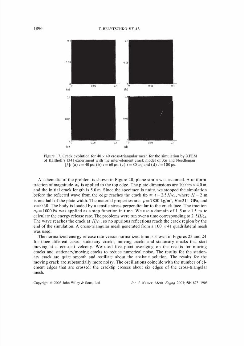
Figure 17. Crack evolution for 40× 40 cross-triangular mesh for the simulation by XFEMof Kaltho’s [34] experiment with the inter-element crack model of Xu and Needleman
[3]: (a) t = 40 s; (b) t = 60 s; (c) t = 80 s; and (d) t =100 s.
A schematic of the problem is shown in Figure 20; plane strain was assumed. A uniformtraction of magnitude 0 is applied to the top edge. The plate dimensions are 10 :0 m× 4:0 m,and the initial crack length is 5:0 m. Since the specimen is ÿnite, we stopped the simulation
before the reected wave from the edge reaches the crack tip at t = 2:5 H=cd, where H = 2 m
is one half of the plate width. The material properties are: = 7800 kg= m3
, E =211 GPa, and = 0:30. The body is loaded by a tensile stress perpendicular to the crack face. The traction0 = 1000 Pa was applied as a step function in time. We use a domain of 1 :5 m× 1:5 m tocalculate the energy release rate. The problems were run over a time corresponding to 2:5 H=cd.The wave reaches the crack at H=cd, so no spurious reections reach the crack region by theend of the simulation. A cross-triangular mesh generated from a 100 ×41 quadrilateral meshwas used.
The normalized energy release rate versus normalized time is shown in Figures 23 and 24
for three dierent cases: stationary cracks, moving cracks and stationary cracks that startmoving at a constant velocity. We used ÿve point averaging on the results for movingcracks and stationary= moving cracks to reduce numerical noise. The results for the station-ary crack are quite smooth and oscillate about the analytic solution. The results for themoving crack are substantially more noisy. The oscillations coincide with the number of el-ement edges that are crossed: the cracktip crosses about six edges of the cross-triangular mesh.
Copyright ? 2003 John Wiley & Sons, Ltd. Int. J. Numer. Meth. Engng 2003; 58:1873–1905
7/30/2019 Dynamic CDynamic crack propagation based on loss of hyperbolicity and a new discontimuous enrichmentrack Pr…
http://slidepdf.com/reader/full/dynamic-cdynamic-crack-propagation-based-on-loss-of-hyperbolicity-and-a-new 25/33
DYNAMIC CRACK PROPAGATION BASED ON LOSS OF HYPERBOLICITY 1897
00 0.05
0.05
0.1
0.1
0
0.05
0.1
0
0.05
0.1
0
0.05
0.1
(a)
0 0.05 0.1
(c)0 0.05 0.1
(d)
0 0.05 0.1
(b)
Figure 18. Crack evolution for 80× 80 cross-triangular mesh for the simulation by XFEMof Kaltho’s [34] experiment with the inter-element crack model of Xu and Needleman
[3]: (a) t = 40 s; (b) t = 60 s; (c) t = 80 s; and (d) t =100 s.
2 3 4 5 6 7 8 9 10
x 10-5
0
500
1000
1500
2000
2500
3000
Time (s)
C r a c k P r o p a g a t i o n S p e e d ( m / s )
40x40 mesh80x80 mesh
5.0 m
σ0
2.0 m
10.0 m
4.0 m = 2 H
Figure 19. Crack propagation speed for dier-ent meshes for the simulation by XFEM of Kaltho’s [34] experiment with the inter-element
crack model of Xu and Needleman [3].
Figure 20. Finite discrete model used for mod-elling the inÿnite plate with a semi-inÿnite crack.
Copyright ? 2003 John Wiley & Sons, Ltd. Int. J. Numer. Meth. Engng 2003; 58:1873–1905
7/30/2019 Dynamic CDynamic crack propagation based on loss of hyperbolicity and a new discontimuous enrichmentrack Pr…
http://slidepdf.com/reader/full/dynamic-cdynamic-crack-propagation-based-on-loss-of-hyperbolicity-and-a-new 26/33
1898 T. BELYTSCHKO ET AL.
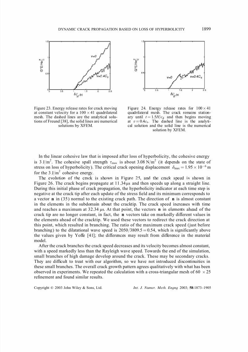
Figure 21. Energy release rates for 100× 41cross-triangular mesh. The dashed lines areanalytical solutions; the solid lines are the
numerical solutions.
Figure 22. Energy release rates for 100× 41cross-triangular mesh. The crack remains station-ary until t = 1:5 H=cd and then begins moving at
v = 0:4cs. The dashed line is the analytical solu-tion, and the solid line is the numerical solution.
We also solved the problem with a 100×41 mesh of quadrilateral elements; the ele-ment is described in Chen [39]. The normalized energy release rate versus normalized timeis shown in Figures 21 and 22 for three dierent cases: stationary cracks, moving cracksand stationary= moving cracks. We used a ÿve point ÿlter on results for moving cracks andstationary= moving cracks to reduce numerical noise.
The results in Figure 22 for a crack moving at constant velocity and at rest comparevery well with the analytical solution, although the latter shows some downward drift toward
the end. Overall the solutions are relatively free of noise. When the crack suddenly startsmoving, as can be seen from Figure 24, there is substantial overshoot at the time of theinitiation of crack motion. This has also been the case for meshfree solutions [32]. However,the quadrilateral element solutions on the whole are substantially better than the triangular element solutions.
6.3. Crack branching by loss of hyperbolicity criterion
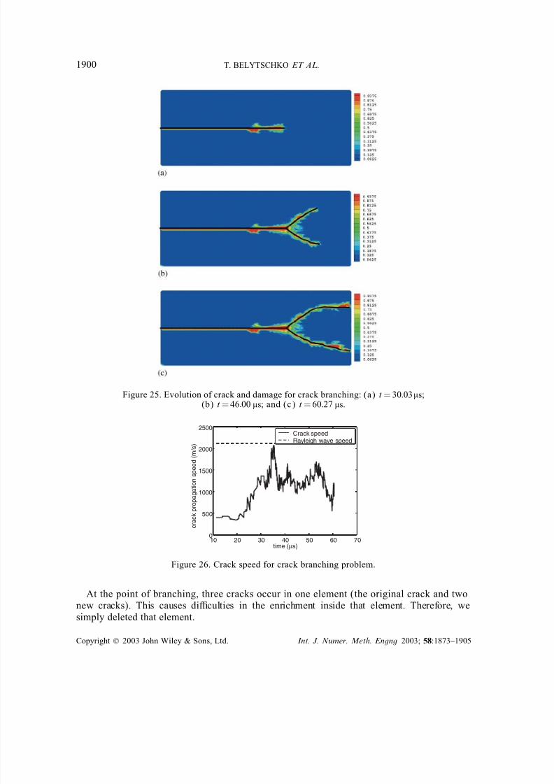
This example concerns the propagation of a crack in a prenotched specimen shown in Figure20 but by the loss of hyperbolicity criterion described in Section 4. The rectangular specimenis of length of 0:1 m and width 0:04 m. Initially a horizontal crack spans from the left edgeto the centre of the plate. Tensile tractions ( = 1 MPa) are applied on the top and the bottom
edges.Material constants are = 2450 kg= m
3, E = 32 GPa, = 0:2. We used the Lemaitre [40]
damage model (see Appendix C). The damage parameters are A = 1:0, B = 7300 and D0= 8:5
× 10−5. The initial dilatational wave speed (with D =0) is cd = 3809:5 m= s; the shear wavespeed cs = 2332:8 m= s; the Rayleigh wave speed cR = 2119:0 m= s. A 50× 21 cross triangular mesh was used with implicit–explicit time integration with a Courant number of 0.4. The totalsimulation time is 61 s.
Copyright ? 2003 John Wiley & Sons, Ltd. Int. J. Numer. Meth. Engng 2003; 58:1873–1905
7/30/2019 Dynamic CDynamic crack propagation based on loss of hyperbolicity and a new discontimuous enrichmentrack Pr…
http://slidepdf.com/reader/full/dynamic-cdynamic-crack-propagation-based-on-loss-of-hyperbolicity-and-a-new 27/33
DYNAMIC CRACK PROPAGATION BASED ON LOSS OF HYPERBOLICITY 1899
Figure 23. Energy release rates for crack movingat constant velocity for a 100× 41 quadrilateralmesh. The dashed lines are the analytical solu-
tions of Freund [38], the solid lines are numericalsolutions by XFEM.
Figure 24. Energy release rates for 100× 41quadrilateral mesh. The crack remains station-ary until t = 1:5 H=cd and then begins moving
at v = 0:4cs. The dashed line is the analyti-cal solution and the solid line is the numericalsolution by XFEM.
In the linear cohesive law that is imposed after loss of hyperbolicity, the cohesive energy
is 3 J= m2
. The cohesive spall strength max is about 3:08 N= m2
(it depends on the state of stress on loss of hyperbolicity). The critical crack opening displacement max = 1:95× 10−6 m
for the 3 J= m2
cohesive energy.The evolution of the crack is shown in Figure 25, and the crack speed is shown in
Figure 26. The crack begins propagate at 11:34s and then speeds up along a straight line.During this initial phase of crack propagation, the hyperbolicity indicator at each time step isnegative at the crack tip after each update of the stress ÿeld and its minimum corresponds toa vector n in (35) normal to the existing crack path. The direction of n is almost constantin the elements in the subdomain about the cracktip. The crack speed increases with timeand reaches a maximum at 32:34 s. At that point, the vectors n in elements ahead of thecrack tip are no longer constant, in fact, the n vectors take on markedly dierent values inthe elements ahead of the cracktip. We used these vectors to redirect the crack direction atthis point, which resulted in branching. The ratio of the maximum crack speed (just before
branching) to the dilatational wave speed is 2050= 3809:5 = 0:54, which is signiÿcantly abovethe values given by Yoe [41]; the dierences may result from dierence in the materialmodel.
After the crack branches the crack speed decreases and its velocity becomes almost constant,with a speed markedly less than the Rayleigh wave speed. Towards the end of the simulation,small branches of high damage develop around the crack. These may be secondary cracks.They are dicult to treat with our algorithm, so we have not introduced discontinuities inthese small branches. The overall crack growth pattern agrees qualitatively with what has beenobserved in experiments. We repeated the calculation with a cross-triangular mesh of 60 × 25reÿnement and found similar results.
Copyright ? 2003 John Wiley & Sons, Ltd. Int. J. Numer. Meth. Engng 2003; 58:1873–1905
7/30/2019 Dynamic CDynamic crack propagation based on loss of hyperbolicity and a new discontimuous enrichmentrack Pr…
http://slidepdf.com/reader/full/dynamic-cdynamic-crack-propagation-based-on-loss-of-hyperbolicity-and-a-new 28/33
1900 T. BELYTSCHKO ET AL.
Figure 25. Evolution of crack and damage for crack branching: (a) t = 30:03s;(b) t = 46:00 s; and (c) t = 60:27 s.
10 20 30 40 50 60 700
500
1000
1500
2000
2500
time (µ
s)
c r a c k p r o p a g a t i o n s p e e d ( m / s )
Crack speedRayleigh wave speed
Figure 26. Crack speed for crack branching problem.
At the point of branching, three cracks occur in one element (the original crack and twonew cracks). This causes diculties in the enrichment inside that element. Therefore, wesimply deleted that element.
Copyright ? 2003 John Wiley & Sons, Ltd. Int. J. Numer. Meth. Engng 2003; 58:1873–1905
7/30/2019 Dynamic CDynamic crack propagation based on loss of hyperbolicity and a new discontimuous enrichmentrack Pr…
http://slidepdf.com/reader/full/dynamic-cdynamic-crack-propagation-based-on-loss-of-hyperbolicity-and-a-new 29/33
DYNAMIC CRACK PROPAGATION BASED ON LOSS OF HYPERBOLICITY 1901
It should be kept in mind that the algorithm for the continuum= crack transition assumes ahigh degree of the smoothness in the path of the crack. This precludes any roughness fromdeveloping in the crack path. Thus the branches in the damage zones may indicate that smallareas of instability develop at intervals around the crack path. These may correspond to the
roughening that has been observed in experiments, e.g. in Ravichandran and Knauss [42].
7. CONCLUSIONS
A methodology has been developed for treating dynamic crack growth by the extended ÿniteelement method (XFEM). In this method, the discontinuity of the crack is represented in theÿnite element approximation by a discontinuous partition of unity enrichment. This enables themethod to treat arbitrary crack growth without remeshing. To extend XFEM to dynamic crack
propagation, a new technique for treating elements that contain crack tips was developed. Inthis new technique, the velocity ÿeld of the element containing the crack tip can changesmoothly from a partially cut element to a fully cut element. By contrast, in previous XFEMenrichments for cracks, the motion of a partially cut element was not consistent in the limitwith a fully cut element, i.e. in the previous XFEM methods, the enrichment resulting frommoving the cracktip to an edge of the element did not correspond with the enrichment of afully cut element. This new technique has been applied to higher order elements by Zi andBelytschko [24].
Results were obtained for several problems. The results matched certain features of exper-iments quite well and overall seem quite promising. Substantially less mesh dependence wasobserved than in the inter-element crack model of Reference [3]. We were not entirely satisÿedwith the quality of the computations with regards to smoothness and quantitative measures.As could be seen from comparison with the analytic energy release rates, the passage of
the wave through element edges still introduces substantial oscillations. These oscillations arealso evident in the cracktip velocity in the simulations of the Kaltho’s experiment and inthe prenotched specimen under tension. Some of this might stem from the explicit–implicitintegration, but this facet requires further research.
In comparing the method to existing methods such as inter-element crack methods, therelative complexity of the methods should be borne in mind. Overall, this method is some-what more complex than inter-element crack methods; the stable time step of the latter isnot eected by the passage of the crack and the elements are never modiÿed. Thus theincreased accuracy of the present method comes at the cost of a moderate increase incomplexity.
The loss of hyperbolicity criterion for propagating the crack appears to be a promisingdirection. This criterion is very attractive for modelling crack growth because it ÿts naturally
with a material model. When hyperbolicity is lost in a rate-independent material model, thena computation cannot continue with a continuum model, since the strain localizes to a set of measure zero occurs. Even with a rate-dependent model, loss of hyperbolicity of the principal
part of the partial dierential equation results in local exponential growth of strain whichwould require exorbitant mesh reÿnement to resolve. Thus the transition to a discontinuousÿeld is essential in a rate-independent model, and advantageous, though not essential, in arate-dependent model.
Copyright ? 2003 John Wiley & Sons, Ltd. Int. J. Numer. Meth. Engng 2003; 58:1873–1905
7/30/2019 Dynamic CDynamic crack propagation based on loss of hyperbolicity and a new discontimuous enrichmentrack Pr…
http://slidepdf.com/reader/full/dynamic-cdynamic-crack-propagation-based-on-loss-of-hyperbolicity-and-a-new 30/33
1902 T. BELYTSCHKO ET AL.
Furthermore, the transition to a discontinuity by the loss of hyperbolicity criterion provides both the crack speed and the crack direction. Thus it provides a natural closure for the dynamiccrack propagation problem. The crack propagation speeds we observed in the calculationsreported here were quite consistent with experimental results: they were always less than the
Rayleigh wave velocity for the material. Similarly, the qualitative pattern of the crack pathsagreed with experimental observations.
This suggests a new paradigm for crack and material modelling: the development of materialmodels that not only predict the right behaviour in the stable regime but correctly predict thetransition to material instability, i.e. cracking or shear banding. It should be noted that drivinga crack by loss of hyperbolicity diers from a cohesive law. A cohesive law can govern certainaspects of crack propagation, but, as pointed out in the paper, it does not provide closure for the crack propagation problem unless a discretization is introduced. Material models have sofar been little tested for their validity in both the stable and unstable regimes. In fact, crack models are usually driven independent of the material model, for example by stress intensityfactors, energy release rates or cohesive stress criteria. The ability of constitutive models to
predict the correct crack velocity and direction to our knowledge has not been examined inany depth.
APPENDIX A: MAXIMUM TENSILE STRESS CRITERION
The maximum tensile stress criterion determines if a crack should propagate by comparingthe maximum tensile stress value in the element ahead of the crack tip to a prescribed pa-rameter max. Once the maximum tensile stress exceeds the tensile strength max, the cracktipis advanced into the next element normal to the maximum tensile stress direction until thecrack tip reaches the element boundary. In practice, we found that the crack angle provided
by this criterion sometimes leads to erratic crack paths. Therefore we used the average value
of the stress ÿelds in several elements ahead of crack tip to determine the crack direction.
APPENDIX B: INTER-EDGE COHESIVE MODEL
In the computations with the inter-element crack method, the cohesive model of Xu and Needleman [3] was used. In this model the traction across the cohesive surface is given by
T=@
@T(B1)
where T is the displacement jump across the cohesive interface and is the cohesive potential[3, 43]:
(T) = n + ne(−n = n )
1 − r +
n
n
1 − q
r − 1−
q +r − q
r − 1
n
n
e(−2
t = 2t )
(B2)
where the subscripts n and t denote the normal and tangential components, respectively. InEquation (B2),
n = emaxn t =
e= 2maxt (B3)
Copyright ? 2003 John Wiley & Sons, Ltd. Int. J. Numer. Meth. Engng 2003; 58:1873–1905
7/30/2019 Dynamic CDynamic crack propagation based on loss of hyperbolicity and a new discontimuous enrichmentrack Pr…
http://slidepdf.com/reader/full/dynamic-cdynamic-crack-propagation-based-on-loss-of-hyperbolicity-and-a-new 31/33
DYNAMIC CRACK PROPAGATION BASED ON LOSS OF HYPERBOLICITY 1903
where n and t are the normal and tangential separation work, respectively, and max
and max are the cohesive strength in the normal and tangential directions, respectively, andn and t are the corresponding characteristic lengths.
q = t
n
r = ∗n
n
(B4)
In the above ∗n is the value of n after complete shear separation. The cohesive tractions arethen obtained by
T n =−n
n
e(−n= n )
n
n
e(−2t = 2
t ) +1 − q
r − 1[1 − e(−2
t = 2t )]
r − n
n
T t =−n
n
2
n
t
t
t
q +
r − q
r − 1
n
n
e(−n = n )e(−2
t = 2t ) (B5)
APPENDIX C: LEMAITRE’S DAMAGE MODEL
The damage model we used was developed by Lemaitre [40] for an isotropic linear elasticvirgin material. The stress–strain law is given as
ij = (1 − D)C ijklkl D ∈ [0; 1] (C1)
where D is a scalar that represents the extent of damage. The damage evolution law is
D( ) = 1 − (1 − A) D0−1 − Ae− B( − D0
) (C2)
where is the eective strain deÿned by
=
3
i=1
2i H (i) (C3)
where H ( x) is the Heaviside function deÿned in Equation (15), A and B are characteristic parameters of the material; D0
is the initial damage threshold strain.
ACKNOWLEDGEMENT
The authors would like to acknowledge the support of the Oce of Naval Research.
REFERENCES
1. Bazant ZP, Belytschko T. Wave propagation in a strain-softening bar: Exact solution. Journal of EngineeringMechanics (ASCE) 1985; 111(3):381–389.
2. Belytschko T, Wang X-J, Bazant ZP, Hyun Y. Transient solutions for one-dimensional problems with strainsoftening. Journal of Applied Mechanics (ASME) 1987; 54(3):513–518.
3. Xu X-P, Needleman A. Numerical simulations of fast crack growth in brittle solids. Journal of the Mechanicsand Physics of Solids 1994; 42:1397–1434.
Copyright ? 2003 John Wiley & Sons, Ltd. Int. J. Numer. Meth. Engng 2003; 58:1873–1905
7/30/2019 Dynamic CDynamic crack propagation based on loss of hyperbolicity and a new discontimuous enrichmentrack Pr…
http://slidepdf.com/reader/full/dynamic-cdynamic-crack-propagation-based-on-loss-of-hyperbolicity-and-a-new 32/33
1904 T. BELYTSCHKO ET AL.
4. Camacho GT, Ortiz M. Computational modeling of impact damage in brittle materials. International Journal of Solids and Structures 1996; 33:2899–2938.
5. Ortiz M, Pandolÿ A. Finite-deformation irreversible cohesive elements for three-dimensional crack-propagationanalysis. International Journal for Numerical Methods in Engineering 1999; 44:1267–1282.
6. Belytschko T, Fish J, Englemann B. A ÿnite element method with embedded localization zones. Computer
Methods in Applied Mechanics and Engineering 1988; 70:59–89.7. Simo JC, Oliver J, Armero F. An analysis of strong discontinuities induced by strain-softening in rate-
independent inelastic solids. Computational Mechanics 1993; 12:277–296.8. Dvorkin EN, Cuitino AM, Gioia G. Finite elements with displacement interpolated embedded localization lines
insensitive to mesh size and distortions. International Journal for Numerical Methods in Engineering 1990;30:541–564.
9. Jirasek M. Comparative study on ÿnite elements with embedded discontinuities. Computer Methods in Applied Mechanics and Engineering 2000; 188:307–330.
10. Belytschko T, Black T. Elastic crack growth in ÿnite elements with minimal remeshing. International Journal for Numerical Methods in Engineering 1999; 45(5):601–620.
11. Moes N, Dolbow J, Belytschko T. A ÿnite element method for crack growth without remeshing. International Journal for Numerical Methods in Engineering 1999; 46(1):133–150.
12. Dolbow J, Moes N, Belytschko T. Discontinuous enrichment in ÿnite elements with a partition of unity method.Finite Elements in Analysis and Design 2000; 36(3):235–260.
13. Belytschko T, Moes N, Usui S, Parimi C. Arbitrary discontinuities in ÿnite elements. International Journal forNumerical Methods in Engineering 2001; 50(4):993–1013.
14. Wells GN, de Borst R, Sluys LJ. A consistent geometrically non-linear approach for delamination. International Journal for Numerical Methods in Engineering 2002; 54:1333–1355.
15. Remmers JJC, de Borst R, Needleman A. A cohesive segments method for the simulation of crack growth.Computational Mechanics 2003; 31:69–77.
16. Gao H, Klein P. Numerical simulation of crack growth in an isotropic solid with randomized internal cohesive bonds. Journal of the Mechanics and Physics of Solids 1998; 42(6):187–218.
17. Oliver J, Huespe AE, Pulido MDG, Samaniego E. On the strong discontinuity approach in ÿnite deformationsettings. International Journal for Numerical Methods in Engineering 2003; 56:1051–1082.
18. Peerlings RHJ, de Borst R, Brekelmans WAM, Geers MGD. Localisation issues in local and nonlocal continuumapproaches to fracture. European Journal of Mechanics – A= Solids 2002; 21:175–189.
19. Belytschko T, Liu WK, Moran B. Nonlinear Finite Elements for Continua and Structures. Wiley: Chichester,2000.
20. Marsden JE, Hughes TJR. Mathematical Foundations of Elasticity. Prentice-Hall, Dover: Englewood Clis, NJ, 1983.
21. Armero F, Garikipati K. An analysis of strong discontinuities in multiplicative ÿnite strain plasticity and their relation with the numerical simulation of strain localization in solids. International Journal of Solids and
Structures 1996; 33(20–22):2863–2885.22. Oliver J. Modelling strong discontinuities in solid mechanics via strain softening constituitive equations, part 1:
fundamentals. part 2: numerical simulation. International Journal for Numerical Methods in Engineering 1996;39:3575–3624.
23. Chessa J, Wang H, Belytschko T. On the construction of blending elements for local partition of unity enrichedÿnite elements. International Journal for Numerical Methods in Engineering 2003; 57(7):1015–1038.
24. Zi G, Belytschko T. New crack-tip elements for xfem and applications to cohesive cracks. International Journal for Numerical Methods in Engineering 2003; 57:2221–2240.
25. Barenblatt G. The mathematical theory of equilibrium of cracks in brittle fracture. Advances in Applied Fracture1962; 7:55–129.
26. Dugdale D. Yielding of steel sheets containing slits. Journal of the Mechanics and Physics of Solids 1960;8:100–108.
27. Hillerborg A, ModÃeer M, Peterson PE. Analysis of crack formation and crack growth in concrete by means of fracture mechanics and ÿnite elements. Cement and Concrete Research 1976; 6:773–782.
28. Planas J, Elices M. Nonlinear fracture of cohesive materials. International Journal of Fracture 1991; 51:139–157.
29. Pandolÿ A, Guduru PR, Ortiz M. Three dimensional cohesive-element analysis and experiments of dynamicfracture in c300 steel. International Journal of Solids and Structures 2000; 37:3733–3760.
30. Pandolÿ A, Krysl P, Ortiz M. Finite element simulation of ring expansion and fragmentation: The capturingof length and time scales through cohesive models of fracture. International Journal of Fracture 1999; 95:279–297.
31. Papoulia KD, Sam CH, Vavasis SA. Time continuity in cohesive ÿnite element modelling. International Journal for Numerical Methods in Engineering 2003; 58:679–701.
32. Belytschko T, Tabbara M. Dynamic fracture using element-free Galerkin methods. International Journal forNumerical Methods in Engineering 1996; 39:923–938.
Copyright ? 2003 John Wiley & Sons, Ltd. Int. J. Numer. Meth. Engng 2003; 58:1873–1905
7/30/2019 Dynamic CDynamic crack propagation based on loss of hyperbolicity and a new discontimuous enrichmentrack Pr…
http://slidepdf.com/reader/full/dynamic-cdynamic-crack-propagation-based-on-loss-of-hyperbolicity-and-a-new 33/33
DYNAMIC CRACK PROPAGATION BASED ON LOSS OF HYPERBOLICITY 1905
33. Hughes TJR, Liu WK. Implicit–explicit ÿnite elements in transient analysis: implementation and numericalexamples. Journal of Applied Mechanics (ASME) 1978; 45:375–378.
34. Kaltho JF, Winkler S. Failure mode transition at high rates of shear loading. International Conference onImpact Loading and Dynamic Behavior of Materials 1987; 1:185–195.
35. Lee YJ, Freund LB. Fracture initiation due to asymmetric impact loading of an edge cracked plate. Journal of
Applied Mechanics (ASME) 1990; 57:104–111.36. Decker RF. Source Book on Maraging Steels. American Society for Metals: Cleveland, OH, 1979.37. Liu Y, Murakamim S, Kanagawa Y. Mesh-dependence and stress singularity in ÿnite element analysis of creep
crack growth by continuum damage mechanics approach. European Journal of Mechanics – A= Solids 1994;13:395–417.
38. Freund LB. Crack propagation in an elastic solid subjected to general loading. 3. stress wave loading. Journal of the Mechanics and Physics of Solids 1973; 21(2):47–61.
39. Chen H. Enriched ÿnite element methods and its applications. Ph.D. Thesis, 2003.40. Lemaitre J. Evaluation of dissipation and damage in metal submitted to dynamic loading. Proceedings ICM 1,
1971.41. Yoe EH. The moving Grith crack. Philosophical Magazine 1951; 42:739–750.42. Ravichandran G, Knauss WG. A ÿnite elastostatic analysis of bimaterial interface cracks. International Journal
of Fracture 1989; 39(1–3):235–253.43. Xu X-P, Needleman A. Void nucleation by inclusion debonding in a crystal matrix. Modelling and Simulation
in Materials Science and Engineering 1993; 1:111–132.
Copyright ? 2003 John Wiley & Sons, Ltd. Int. J. Numer. Meth. Engng 2003; 58:1873–1905


![arXiv:1807.05946v4 [math.AG] 28 Jan 2020 · algebraic, differential, and arithmetic geometry coincide: Brody hyperbolicity (no entire holomor-phic curves), arithmetically hyperbolicity](https://img.pdfslide.us/doc/110x75/5fb96b90782a89050a02e48d/arxiv180705946v4-mathag-28-jan-2020-algebraic-diierential-and-arithmetic.jpg)