QEDQueen’s Economics Department Working Paper No. 1358

Dynamic Capital inflow transmission of monetary policy toemerging markets

Adugna OlaniQueen’s University

Department of EconomicsQueen’s University

94 University AvenueKingston, Ontario, Canada

K7L 3N6

3-2016

Dynamic Capital Inflow Transmission of MonetaryPolicy to Emerging Markets

Adugna Olani∗

March 10, 2017

Abstract

This paper analyzes the dynamic and size effects of the U.S. monetary policy shock, aproxy for advanced economies’ monetary policy shock, as well as domestic monetaryand exchange rate shocks on gross foreign direct and portfolio investment inflows toemerging markets. It uses panel and country-specific structural vector auto-regressionsto analyze and compare the dynamic, size, and differential impacts of the shocks on eachinflow category. Foreign direct investment inflow’s response to policy shocks is weakbut persistent while that of foreign portfolio investment is strong and on impact. Theimplication is that macro-prudential and capital control policies may be more effectivewhen they are directed at portfolio inflows. In addition to providing a richer dynamicstructure, the use of structural vector auto-regressions provides a clearer comparison of“push” and “pull” factors on financial flows via forecast error variance decomposition.Although the U.S. monetary policy explains a significant variation in both gross inflows,this paper does not find a consistent evidence of “push” over “pull” factors in eithercapital inflow type or across the countries.

Key Words: Monetary policy, Capital Flow, Emerging Market, Exchange Rate,Interest RateJEL classification codes: E52 F32 E43 E58 F37

∗Department of Economics, Queen’s University, 94 University Avenue, Kingston, Ontario, Canada K7L3N6. E-mail: olania@econ.queensu.ca. I am grateful to Allen Head, Beverly Lapham, and Huw Lloyd-Ellisfor their guidance and invaluable comments. I have received important comments from seminar participantsat CEA meeting in Toronto, Queen’s Ph.D. students seminar series, Brown Bags for CEAs, and the EmpiricalMacro reading group at Queen’s University.

1 Introduction

This paper provides an empirical analysis of the effect of the U.S. monetary policy (MP) as

well as domestic monetary and exchange rate shocks on the dynamics, size, and composition

gross capital inflows to emerging markets (EMs). Increased cross-border gross asset and

liability positions in the last two decades have potentially improved risk-sharing of the EMs

with the rest of the world (Lane and Milesi-Ferretti, 2007). On the other hand, adverse

shocks can be transmitted through financial flows to EMs. However, the dynamic and size

effects of policy changes on cross-border capital inflow categories have been less explored.

This paper seeks to increase our understanding in this aspect.

Specifically, this paper has a threefold purpose. First, it uses panel and country-specific

structural vector auto-regression (SVARs) to show the differential dynamic and size effects

of the U.S. conventional MP, a proxy for advanced economies’ MP, on gross foreign direct

investment (FDI) and foreign portfolio investment (FPI) inflows.1 Secondly, it analyses

the dynamic and size effects of domestic monetary and exchange rate policies on the two

categories of inflows. Thirdly, it revisits the domestic pull versus external push factors debate

for the two categories of capital inflows. Pull factors are domestic factors that attract a

foreign investor to invest in EMs while push factors are factors in the home country of the

foreign investor that induces her to invest in the EMs. SVARs allow quantitative comparison

of the push and pull factors via forecast error variance decomposition which is not generally

available in cross-country panel data regressions.

Recent and previous studies, mainly due to data limitations, used panel data regressions

to analyze the effect of policies on capital flows. With few exceptions, they mainly used

the total or net capital inflows data to multiple countries. A few examples are Rey (2015),

Bruno and Shin (2015) Lim et al. (2014), MacDonald (2015), Ahmed and Zlate (2014),

Gourinchas and Rey (2013), Gourinchas and Jeanne (2013), Forbes and Warnock (2012),

1Foreign Direct Investment (FDI) is defined as investment involving at least 10% ownership in EMsfirms. It reflects investment relationships based on control and influence. On the other hand, Foreign Port-folio Investment (FPI) involves cross-border transactions and positions involving debt or equity securities.The main differences between the two are in ownership (the degree of managerial control), liquidity, andreversibility.

Fratzscher (2012). However, panel data regressions, unlike vector auto-regressions, are un-

able to provide the dynamics of capital flows and their time series characteristics after shocks

to macroeconomic policies.

In this paper, using panel data and country-specific SVARs, I provide a richer dynamic

and size effects of policies on the categories of capital inflows to EMs. SVAR estimations

also have a readily available tool to compare the push and pull factors. Understanding the

categories of gross capital inflows, instead of the total or net flows, is important because the

different categories of flows are imperfect substitutes and are different in their nature and

purposes. Similarly, understanding the responses of each inflow category in each country is

important as there may be heterogeneity across countries. Therefore, I compare and contrast

the two categories of inflows to EMs, and examine the differences and similarities in their

responses to policy shocks across the EM countries.

The U.S. conventional MP can be used as a proxy for the advanced economies’ monetary

policy.2 Particularly, I use the federal fund’s shadow rate (ffs) by Wu and Xia (2016) as a

monetary policy stance of the U.S. The federal fund’s rate (ff) and the U.S. 3-Month T-bill

rates were essentially zero from December 16, 2008, to December 15, 2015. Due to this zero

lower bound (ZLB) any coefficient estimate of the effect of conventional policy using the

ff will be biased as the ff data is censored.3 The ZLB will also affect the term-structure

measure, since a compression in the yield spread may reflect either a genuine change in term

structure, or simply the inability of the observed federal fund’s rate to go below zero. The

ffs is an approximation that makes a nonlinear term-structure model tractable for analysis

of an economy operating near the ZLB for interest rates. For the period before the ZLB,

both ffs and ff are identical.

Studying the transmission of advanced economies’ MP shocks to EMs through capital

inflows is paramount. Historically, the effects of advanced economies’ MP shocks and their

2Detailed reasoning as to why this is the case is provided in Section 2.3Liu et al. (2011) and Kilian (2013) provide reviews and explain the special challenges in the SVAR

estimation associated with periods when the interest rate is pressed against the zero lower bound. Fernandez-Villaverde et al. (2015) argues for the importance of explicitly considering nonlinearities with a zero lowerbound (ZLB) on the nominal interest rate.

2

capital inflow consequences have been significant.4 Recently, after the financial crisis of

the 2008 and the implementation of unconventional MP in the U.S., the central banks of

emerging economies have shown concern regarding the impact of quantitative easing (QE)

and its tapering. For example, Rey (2015) contends that MP in the “center country” is an

important determinant of capital flows, and greater MP coordination among central banks

may be necessary.5

I analyze gross FDI and FPI inflows to EMs as they are different in nature and are

imperfect substitutes, instead of focusing only on their aggregates or net-flows. In general,

studying several disaggregates of financial flow variables is justified by many reasons. First,

there are differences in the investors’ behavioral decision-making process in investing in

categories of inflows and outflows. Secondly, long term and short term investments are

determined by different underlying factors. For example, Janus and Riera-Crichton (2013)

finds studying net flows ignores that the causes and the effects of outflows from an economy

may be distinct from those of inflows. Furthermore, international short-term investments in

general and portfolio investments, in particular, are often called “hot money” because they

can be reversed quickly. In contrast, foreign direct investments are a more stable flow of

capital, which is linked more closely to the permanence of the physical capital and is induced

by long-term prospects of the receiving country. Therefore, external or domestic shocks can

affect these flows differently.

There are some more fundamental differences between FDI and FPI inflows. FDI is

an illiquid investment whose determinants are more linked to microeconomic considerations

than the macroeconomic environment. Information asymmetry between managers, owners,

and potential buyers characterize FDI more than FPI. The political atmosphere of the host

4Alejandro (1983) emphasizes the importance of global monetary policy (MP) during the 1930s and1940s in Latin-American countries’ capital inflows and outflows. Eichengreen (1990) relates the historicaltrend in capital inflows before 1914 to the operation of the international gold standard. Calvo et al. (1996)documents that in Latin America episodes of capital inflows during the 1920s and 1978-1981 were related toglobal factors such as cyclical movement in interest rates. According to Adelman (1998) and Calvo (1998) theMexican balance-of-payments crisis of December 1994, also called the Tequila crisis, was related to activitiesat “world money centres.”

5The importance of global monetary policy shocks have been documented in theoretical models such asAguiar and Gopinath (2007) Mendoza (1991) and which discuss that in economies with a high debt-serviceratio, fluctuations in the world interest rate plays a significant role.

3

country is more critical in FDI decisions than in FPI (Ahlquist, 2006). For example, the

standard deviations (St.dev.) of FDI and FPI inflows to eight large EMs provided in Table

1 shows that FPI inflows are more volatile than FDI inflows in all the EMs considered.

Table 1: Quarterly mean and standard deviation FDI and FPI inflows ( Source: Interna-tional Financial Statistics (IFS))

FDI FPI CorrMean St.dev. CV Mean St. dev CV Corr(FDI,FPI)

Brazil 2.632 1.284 0.488 1.064 2.013 1.892 -0.133India 1.536 0.929 0.605 0.935 1.189 1.272 -0.071

Indonesia 1.084 1.755 1.619 0.937 3.046 3.251 0.431Mexico 0.714 0.327 0.458 0.391 0.814 2.082 -0.314Philipp. 1.148 1.178 1.026 1.340 2.458 1.834 0.239Russia 2.258 1.717 0.760 0.633 3.932 6.212 -0.067

South Africa 0.332 0.638 1.922 0.681 1.03 1.512 -0.283Thailand 3.100 1.942 0.626 1.281 2.398 1.872 -0.162

Notes: Generally, quarterly mean inflow of FDI is larger than that of FPI while the volatility of FPI isgreater than that of FDI. Their correlation coefficient (corr) is generally negative (substitutes). CV denotesthe ratio of St.dev. to Mean

I use panel and country-specific structural vector auto-regressions (SVARS) to examine

the differential effects of U.S. conventional MP as well as EMs’ domestic monetary and

exchange rate shocks on the dynamics and size of the categories gross capital inflows to

EMs. The panel and country-specific SVARs suggest three main findings. First, in response

to tightening of U.S. MP, as the term-structure in the U.S decreases, FPI inflows increase on

impact (dynamics) and strongly (size) while FDI’s increase is persistent but weak. Secondly,

the results indicate that domestic monetary and exchange rate shocks have less impact on

FDI while FPI’s response to the same shocks are on impact and are larger in size. Thirdly,

although the U.S. conventional MP is an important variable in explaining the dynamics of

both categories of capital inflows to EMs, I do not find a strong push over pull factor across

countries in either type of gross inflow. These results are robust to extensive robustness

checks.

The main contributions of this paper are the following. First, unlike previous studies on

cross-border capital flows, it applies panel and country-specific SVARs to provide a richer

dynamics in identifying the effects of MP shocks on the components of gross capital inflows

4

using a newly constructed dataset. Secondly, it contributes to the debate in “push” and

“pull” factors for the categories of capital inflows quantitatively using the forecast error

variance decomposition. Thirdly, it uses the inflows data as a ratio of nominal GDP, and

alternatively, the capital inflow data as an index to arrive at qualitatively similar results.6

The structure of the paper is as follows. Section 2 presents the theoretical framework

for identification and estimation. Section 3 discusses the data. Section 4 first presents

the estimated results of the U.S. conventional monetary as well as domestic monetary and

exchange shocks on the categories of gross capital inflows using SVARs and then discusses the

implied forecast-error variance decomposition. Section 5 discusses robustness of the results.

Section 6 provides concluding remarks, policy implications and suggestions for future works.

2 Theoretical Framework for Identification and Esti-

mation

Let an SVAR in K variables that contemporaneously affect each other be defined as:

B0Yt = B1Yt−1 + ...+BpYt−p + εt (1)

where Yt is a K × 1 vector of endogenous variables and εt is a K × 1 vector of error terms,

Bi’s are a K ×K matrices of parameters for i = 0, 1, ...p, E(εt) = 0, and E(εtε′t) = Σε. εt is

assumed to be uncorrelated orthogonal structural shocks. Deterministic regressors have been

suppressed for notational convenience. The coefficients in Bi’s cannot be directly estimated.

However, we can recover them from the estimation of reduced form VARs of the variables

whose error terms are denoted as vector et in Equation 2.

Yt = A1Yt−1 + ...+ ApYt−p + et (2)

6Using both data series and checking the consistency helps to avoid a spurious increase in the inflowsratio during recessions as GDP decreases. The analysis using the index data is reported as a robustnesscheck in the appendix.

5

where A1 = B−10 B1, ... Ap = B−10 Bp, et = B−10 εt. Then the contemporaneous matrix B0 is

identified and recovered from the variance-covariance matrix of the reduced form estimation

by imposing recursive restrictions based on economic theories.

The variables used in the estimations below are the U.S. federal funds shadow rate (ffst),

the logarithm of the domestic industrial production index (yt), the logarithm of the domestic

consumer price index (pt), the domestic short-term interest rate (rt), the logarithm of the

nominal exchange rate (in domestic currency per the U.S. dollar, (et)), and the capital inflow

variable as a ratio of GDP. Alternatively, I will also estimate the SVAR by replacing ffst by

the term structure. The term-structure (termt) is the U.S. 10-Year T-Bill minus the ffst.

The ordering of the benchmark recursive structure is a vector Yt where the order of the

variables is given as

Yt = ffst, yt, pt, rt, et, FDIt, and Yt = ffst, FPIt, yt, pt, rt, et (3)

In the estimations of the system for FDI, denoting the K2 elements in B0 by bij, the

relationship in Equations 1 and 2 can be written as:εffsεyεpεrεeεFDI

=

1 0 0 0 0 0b21 1 0 0 0 0b31 b32 1 0 0 0b41 b42 b43 1 0 0b51 b52 b53 b54 1 0b61 b62 b63 b64 b65 1

×effseyepereeeFDI

For FPI, the order is reorganized as denoted in Equation 3.

I use theoretically plausible identification conditions to order the variables in the bench-

mark recursive structure. The block recursive SVAR is ordered such that the least endoge-

nous variable (ffs) comes first and the most endogenous (FDI) later in the order. For

FPI, as changing the portfolio investment position of the foreign investor is a little more

than clicking computer keys away (Calvo et al., 1996), it is ordered as the second variable

immediately after ffs.

The first identification condition is the assumption of a small open economy: a small

open economy does not have a significant effect on the U.S. MP (ffs), a proxy for advanced

6

economies’ MP, while the U.S. MP can affect the macroeconomic variables of the small

open economy. Each EM is a small open economy because the U.S. MP influences the

macroeconomic conditions of EMs. Therefore, the first variable in the ordering is the U.S.

MP, ffs or term, and it is the least endogenous.

The second identification condition is the ordering of y, p, r which is suggested by the

Taylor Rule: central banks target the output gap and inflation in determining the interest

rate. To capture the output gap and inflation, I include a constant and a trend in the

estimation. The trend captures the trend in output data to estimate the output gap while

the constant contains information about the target inflation rate. The Taylor Rule, using

the coefficients in the B0 above and ffs, is given as:

rt = κ1 + κ2(ffst) + b42(pt − p∗) + b43(yt − y) + ert

rt = κ3 + κ4(trend) + κ5(ffst) + b42(pt) + b43(yt) + ert

(4)

where κ′is, b42, and b43 are constants, while p∗ and y are respectively the target inflation rate

and potential output, and ert is the error-term in the respective equation. In addition, the

ordering is plausible because there are delays in the impact of MP on the domestic economy.

Furthermore, a central bank has at its disposal monthly data on aggregate employment,

industrial output, and other indicators of aggregate real economic activity to make interest

rate decisions. It also has substantial amounts of information regarding the price level

(Christiano et al., 1999). The ordering of pt after yt is that contemporaneous feedback from

price to output has a delay as changing output levels may take more time relative to changing

prices. The fourth row is, therefore, a world interest rate augmented Taylor Rule equation.

The third identification condition is that the exchange rate (et) follows rt as suggested by

the uncovered interest rate parity and empirical evidence by Eichanbaum and Charles (1995).

Uncovered interest parity entails risks and elements of speculation in the determination of

exchange rate. The exchange rate is affected by the domestic interest rate. The uncovered

interest rate equation is given as:

E(∆et) = F (∆rt) =⇒ E(et) = F (rt) (5)

7

where E denotes the expectation operator and F denotes the functional relationship.

The fourth identification condition follows a narratiive approach in a similar sense to

Romer and Romer (2004) identification. The narrative is that the FDI inflow must be the

most endogenous variable. FDI inflows are the most endogenous variable because investors

take into account the macroeconomic environment of the small open economy in making

the investment decision. Though I need the contemporaneous feedback effects only, Brooks

et al. (2004) and Bakardzhieva et al. (2010) show that the backward feedback from inflows

to the exchange rate is weak. That is, FDI has no significant effect on exchange rates. Also,

in studies that focus on monetary transmission through financial variables in the domestic

economy caution that the domestic output is affected by the financial variables because

the central banks may be indirectly responding to the effects financial variables. However,

categories of capital flows influence output at different speeds. Thus, because changing the

FPI position can be clicking computer keys away while that is not the case for FDI, I

place FPI after ffs. This ordering is a plausible and simpler identification for cross-border

capital flows.7

Given the above theoretically plausible identification conditions, I use other orderings to

check robustness of the results. In particular, I present a result from an alternative ordering

of ffs, FDI, y, p, r, e and ffs, y, p, r, e, FPI for FDI and FPI, respectively.

The estimated coefficients of the SVARs with possibly non-stationary variables are con-

sistent, and the asymptotic distribution of individual estimated parameters is the standard

normal distribution (See Sims et al. (1990)).8 Phillips (1998) indicates that the results from

such an estimation are consistent estimators of the true impulse responses. In addition, I get

around the potential limitation in data points by estimating the panel as well as country-

specific SVARs with degrees of freedom adjusted coefficients. Phillips and Spencer (2011)

finds that for small samples, as shown in the estimations, degrees of freedom adjustment will

eliminate bias and the bootstrap confidence intervals exhibit improved coverage accuracy. In

7To deal with such problems, Gertler and Karadi (2015) use high-frequency identification (HFI) to inves-tigate domestic MP transmissions. However, in an international capital flow set up, I assume a sufficient lagafter a shock to monetary policy that endogeneity of FDI may not be an issue because such investments takethe time to plan and implement. Furthermore, the effect of capital inflow on domestic output is sluggish.

8See also Hamilton (1994) page 557 for further discussion.

8

the estimated models, Schwarz Bayesian Information Criteria is used to select the maximum

lags to be included in the model.

3 Data

I analyze the two major gross capital inflows: gross FDI and FPI inflows to EMs using

quarterly time-series data from 1990 to 2014, data permitting.9 I analyze quarterly data on

gross FDI and FPI inflows to eight EMs: Brazil, Russia, India, South Africa, Indonesia,

Mexico, the Philippines, and Thailand. Country choice and the length of data was made

based on the availability of data. The data for Brazil, Russia, India, and South Africa span

1995Q1-2013Q4, 1995Q1-2014Q2, 1996Q4-2014Q1 and 1990Q1-2014Q2, respectively.10 The

data for Indonesia, Mexico, Philippines and Thailand span 1993Q1-2014Q2, 1995Q1-2014Q2,

1990Q1-2014Q2 and 1993Q1-2014Q1, respectively.

The primary source of the data is the analytic presentation of the IMF’s Balance of

Payments Statistics Yearbooks (BOP) and International Financial Statistics (IFS) comple-

mented with the countries’ central bank statistics. The presentation of the capital flow data

(in U.S. dollars) for the time series up to 2004Q4 is from BPM5 while the data after 2005Q1

is from BPM6.11 The data is complemented and cross checked with reports of the central

banks of each country as well as the data from Federal Reserve Bank of St. Louis. Each of

the financial flow variables is used as a ratio to nominal GDP (NGDP) in the same quarter,

9Foreign direct investment is a category of cross-border investment associated with a resident in oneeconomy having control or a significant degree of influence on the management of a company that is residentin another economy. Portfolio investment involves cross-border transactions and positions involving debt orequity securities. Thus, the main differences between the two are in ownership (the degree of managerialcontrol), liquidity, and reversibility. The IMF and the World Bank define FDI as “investment to acquire alasting management interest (10% or more of voting stock) in an enterprise operating in an economy otherthan that of the investor. It is the sum of equity capital, reinvestment of earnings, other long-term capital,and short-term capital as shown in the balance of payments”)

10Seven of these countries, except the Phillippines, account for more than 80% of the inflows receipt. ThePhilippines was included because its data was available. China’s data was not available, and it may bedifficult to assume China is a small open economy.

11Until 2004Q4, gross direct and portfolio investment inflows (FDI and FPI) were recorded as a liability(negative number to show the increase in debt of the recipient country) account in the BOP statistics,(BPM5). The data after 2005Q1 is recorded as a positive number. So I changed the sign of the data earlierthan 2005Q1 to be consistent while checking for accuracy. Therefore, the liability account dynamics couldbe due to changes in the real flows or changes in the asset prices and exchange rates.

9

a commonly used measure. The financial flows and NGDP are in the U.S. dollars.12

I use seasonally adjusted FDI and FPI inflows to NGDP ratios, alternatively, their

respective indices calculated from the ratio of each inflow to its 2005Q1 value for robustness,

and the logarithms of y, p, and e. At the beginning of the project, I used both the nominal

and real effective exchange rates, and they did not change the result because of a close to

unity correlation coefficient of the nominal, real, and real-effective exchange rates. Here, the

nominal exchange rates are used for the analysis. The 3-Month T-bill rate or the respective

country’s central bank’s short-rate of is the measure of domestic monetary policy. I use

domestic consumer price index (p) as a measure of the domestic price level. The industrial

production index is our measure of output (y) for Brazil, India, Mexico and Russia. For

Indonesia, I use the manufacturing production index and the real GDP indices for Philip-

pines, South Africa, and Thailand. All the time-series variables except the interest rates are

seasonally adjusted. I use the ffs by Wu and Xia (2016) for the U.S. monetary policy as

indicated in the Introduction section of this paper.

Monetary Policy (MP) shocks that originate from the U.S. can be used as a proxy for

the global MP condition or the advanced economies monetary policy environment. Using

the U.S. MP shock, specifically a shock to the U.S. federal funds shadow rate (ffs) and

the difference between the 10-Year T-Bill and ffs (term-structure), can be a proxy for the

advanced economies’ monetary policy stance. A related literature discusses the justification

for taking the U.S. MP as a proxy for global MP. For example, Gourinchas and Rey (2013)’s

reasoning is that: first, the U.S. is the largest economy in the world and after the Second

World War the U.S. has been a global liquidity provider. Secondly, as the center country,

the U.S. issues the currency used in most international exchanges whether in goods markets

or financial markets. Finally, the role of the center country is not only as a liquidity provider

but also a global insurer. Therefore, the U.S. is usually considered as a source of global

MP or macroeconomic shock. Also, the U.S. dollar is the most liquid international means

of exchange and the currency denomination of U.S. Treasuries, which are held as a reserve

12For further details of the method of recording and differences between BPM5 and BPM6, please see:http://www.imf.org/external/pubs/ft/bop/2014/pdf/GuideFinal.pdf especially, see Box 10.5 of thefinancial account recording for the consistent use of the exchange rate

10

asset across the globe.

The other reason why the U.S. MP can be a proxy for the global MP is that the interest

rates of other advanced economies follow similar trends (are co-integrated and fractionally

co-integrated) to that of the U.S.. Papanyan (2010) empirically verifies that the U.S. is

not affected by the country-specific permanent shocks of Europe or Japan, which further

supports the assumption that U.S. is not a small open economy. Therefore, other advanced

economies are also affected by an exogenous shock that arises from the U.S.

Table 2: Correlation coefficients of advanced economies interest rates

U.K. rate Euribor U.S. 3M U.S. ff US 10Y

U.K. rate 1.0 0.87 0.88 0.89 0.88Euribor 1.0 0.76 0.79 0.76

U.S. 3-Month T-Bill 1.0 1.0 0.87U.S. ff 1.0 0.86

U.S. 10-Year T-Bill 1.0

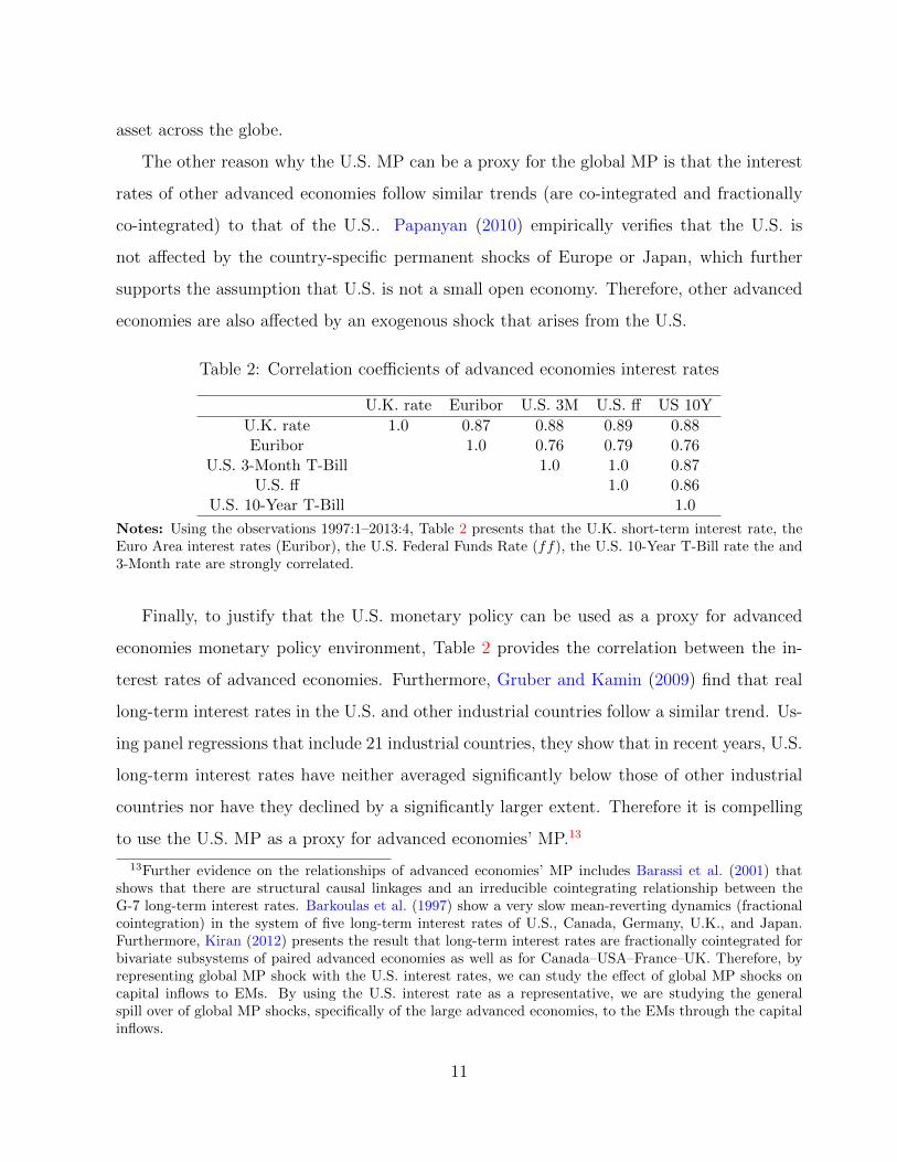
Notes: Using the observations 1997:1–2013:4, Table 2 presents that the U.K. short-term interest rate, theEuro Area interest rates (Euribor), the U.S. Federal Funds Rate (ff), the U.S. 10-Year T-Bill rate the and3-Month rate are strongly correlated.

Finally, to justify that the U.S. monetary policy can be used as a proxy for advanced

economies monetary policy environment, Table 2 provides the correlation between the in-

terest rates of advanced economies. Furthermore, Gruber and Kamin (2009) find that real

long-term interest rates in the U.S. and other industrial countries follow a similar trend. Us-

ing panel regressions that include 21 industrial countries, they show that in recent years, U.S.

long-term interest rates have neither averaged significantly below those of other industrial

countries nor have they declined by a significantly larger extent. Therefore it is compelling

to use the U.S. MP as a proxy for advanced economies’ MP.13

13Further evidence on the relationships of advanced economies’ MP includes Barassi et al. (2001) thatshows that there are structural causal linkages and an irreducible cointegrating relationship between theG-7 long-term interest rates. Barkoulas et al. (1997) show a very slow mean-reverting dynamics (fractionalcointegration) in the system of five long-term interest rates of U.S., Canada, Germany, U.K., and Japan.Furthermore, Kiran (2012) presents the result that long-term interest rates are fractionally cointegrated forbivariate subsystems of paired advanced economies as well as for Canada–USA–France–UK. Therefore, byrepresenting global MP shock with the U.S. interest rates, we can study the effect of global MP shocks oncapital inflows to EMs. By using the U.S. interest rate as a representative, we are studying the generalspill over of global MP shocks, specifically of the large advanced economies, to the EMs through the capitalinflows.

11

4 Results

4.1 Results from panel data structural vector auto-regressions

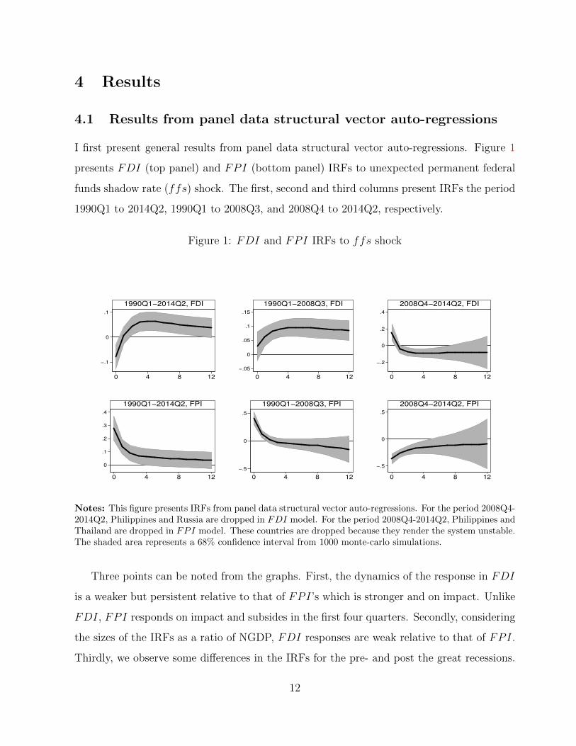
I first present general results from panel data structural vector auto-regressions. Figure 1

presents FDI (top panel) and FPI (bottom panel) IRFs to unexpected permanent federal

funds shadow rate (ffs) shock. The first, second and third columns present IRFs the period

1990Q1 to 2014Q2, 1990Q1 to 2008Q3, and 2008Q4 to 2014Q2, respectively.

Figure 1: FDI and FPI IRFs to ffs shock

−.1

0

.1

0 4 8 12

1990Q1−2014Q2, FDI

−.05

0

.05

.1

.15

0 4 8 12

1990Q1−2008Q3, FDI

−.2

0

.2

.4

0 4 8 12

2008Q4−2014Q2, FDI

0

.1

.2

.3

.4

0 4 8 12

1990Q1−2014Q2, FPI

−.5

0

.5

0 4 8 12

1990Q1−2008Q3, FPI

−.5

0

.5

0 4 8 12

2008Q4−2014Q2, FPI

Notes: This figure presents IRFs from panel data structural vector auto-regressions. For the period 2008Q4-2014Q2, Philippines and Russia are dropped in FDI model. For the period 2008Q4-2014Q2, Philippines andThailand are dropped in FPI model. These countries are dropped because they render the system unstable.The shaded area represents a 68% confidence interval from 1000 monte-carlo simulations.

Three points can be noted from the graphs. First, the dynamics of the response in FDI

is a weaker but persistent relative to that of FPI’s which is stronger and on impact. Unlike

FDI, FPI responds on impact and subsides in the first four quarters. Secondly, considering

the sizes of the IRFs as a ratio of NGDP, FDI responses are weak relative to that of FPI.

Thirdly, we observe some differences in the IRFs for the pre- and post the great recessions.

12

The first two points will generally continue to hold in the country-specific analyses. However,

because of degrees of freedom loss (few data points to analyze), the third point is difficult

to show for each country.

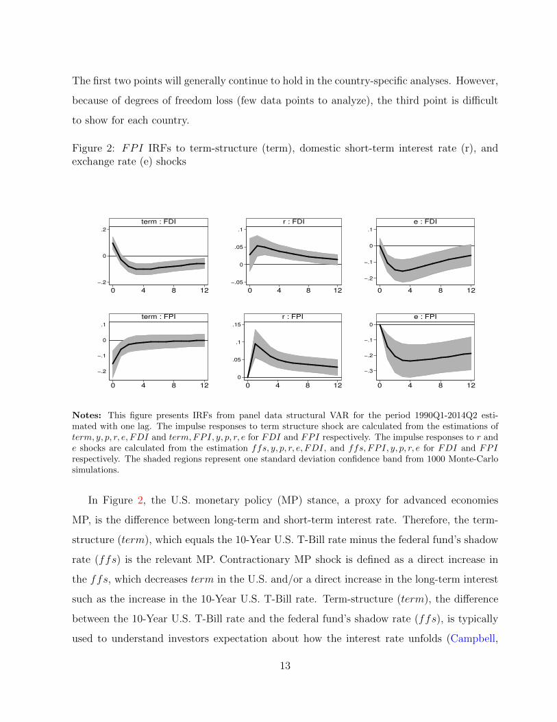
Figure 2: FPI IRFs to term-structure (term), domestic short-term interest rate (r), andexchange rate (e) shocks

−.2

0

.2

0 4 8 12

term : FDI

−.05

0

.05

.1

0 4 8 12

r : FDI

−.2

−.1

0

.1

0 4 8 12

e : FDI

−.2

−.1

0

.1

0 4 8 12

term : FPI

0

.05

.1

.15

0 4 8 12

r : FPI

−.3

−.2

−.1

0

0 4 8 12

e : FPI

Notes: This figure presents IRFs from panel data structural VAR for the period 1990Q1-2014Q2 esti-mated with one lag. The impulse responses to term structure shock are calculated from the estimations ofterm, y, p, r, e, FDI and term,FPI, y, p, r, e for FDI and FPI respectively. The impulse responses to r ande shocks are calculated from the estimation ffs, y, p, r, e, FDI, and ffs, FPI, y, p, r, e for FDI and FPIrespectively. The shaded regions represent one standard deviation confidence band from 1000 Monte-Carlosimulations.

In Figure 2, the U.S. monetary policy (MP) stance, a proxy for advanced economies

MP, is the difference between long-term and short-term interest rate. Therefore, the term-

structure (term), which equals the 10-Year U.S. T-Bill rate minus the federal fund’s shadow

rate (ffs) is the relevant MP. Contractionary MP shock is defined as a direct increase in

the ffs, which decreases term in the U.S. and/or a direct increase in the long-term interest

such as the increase in the 10-Year U.S. T-Bill rate. Term-structure (term), the difference

between the 10-Year U.S. T-Bill rate and the federal fund’s shadow rate (ffs), is typically

used to understand investors expectation about how the interest rate unfolds (Campbell,

13

1996).

Unexpected permanent positive shock to the U.S. short-term interest rate (ffs) increases

cost of borrowing and decreases the margin between long-term and short-term interest rate

(term) in the U.S. making an investment in the emerging markets attractive (Figure 1). In

other words, as the long-term interest rate in the U.S. (U.S. 10-Year T-Bill) increases, the

term-structure in the U.S. increases and capital inflows to the emerging markets decreases

(Figure 2). In addition, an increase in the U.S. short-term interest rate (ffs) typically takes

place when the U.S. economy booms which induce optimistic investors’ investment in EMEs

to increase. Both Figures 1 and 2 show that an unexpected contractionary U.S. conventional

MP, which increase the ffs and/or decrease term, influence FPI on impact and strongly

while the effect is persistent but weak for FDI. In Figure 2 strong response of FPI IRFs

to the domestic interest and exchange rate shocks will generally hold when country-specific

IRFS are considered.

4.2 Results from country-specific structural vector auto-regressions

4.2.1 The dynamic effects of the U.S. monetary policy shocks on FDI and FPI

I continue to use unexpected permanent shocks to the U.S. federal funds shadow rate (ffs)

and the term-structure (term) as a proxy for advanced economies monetary policy shocks.

Here, I analyze the impulse responses of FDI and FPI following the shocks to ffs and

term for each country. I then compare and contrast the two categories of inflows.

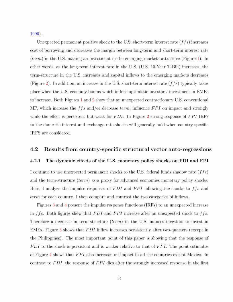
Figures 3 and 4 present the impulse response functions (IRFs) to an unexpected increase

in ffs. Both figures show that FDI and FPI increase after an unexpected shock to ffs.

Therefore a decrease in term-structure (term) in the U.S. induces investors to invest in

EMEs. Figure 3 shows that FDI inflow increases persistently after two-quarters (except in

the Philippines). The most important point of this paper is showing that the response of

FDI to the shock is persistent and is weaker relative to that of FPI. The point estimates

of Figure 4 shows that FPI also increases on impact in all the countries except Mexico. In

contrast to FDI, the response of FPI dies after the strongly increased response in the first

14

two-quarters. As a percent of NGDP, the impulse responses of FPI are stronger relative to

that of FDI (sizes on the vertical axes).

Figure 3: FDI IRFs to ffs shock

−.1−

.05

0.0

5.1

.15

0 4 8 12 16 20

Brazil

−.3

−.2

−.1

0.1

0 4 8 12 16 20

India

−.1

0.1

.2

0 4 8 12 16 20

Russia

−.3

−.2

−.1

0.1

0 4 8 12 16 20

South Africa

−.06

−.04

−.02

0.0

2

0 4 8 12 16 20

Mexico

−.2

−.1

0.1

.2

0 4 8 12 16 20

Indonesia

0.1

.2.3

.4

0 4 8 12 16 20

Philippines

−.1

0.1

.2.3

0 4 8 12 16 20

Thailand

Figure 4: FPI IRFs to ffs shock

0.2

.4.6

0 4 8 12 16 20

Brazil

−.2

0.2

.4.6

0 4 8 12 16 20

India

−.2

0.2

.4.6

0 4 8 12 16 20

Russia

−.1

0.1

.2.3

.4

0 4 8 12 16 20

South Africa

−.1

−.05

0.0

5

0 4 8 12 16 20

Mexico

−.2

0.2

.4

0 4 8 12 16 20

Indonesia

−.1

0.1

.2.3

.4

0 4 8 12 16 20

Philippines

−.2

0.2

.4.6

0 4 8 12 16 20

Thailand

Notes: Figures 3 and 4 present the IRFs of FDI and FPI to ffs shock in a recursive VAR ordered as(ffs, y, p, r, e, FDI) and (ffs, FPI, y, p, r, e) respectively. They are estimated with one standard deviationbootstrap confidence bands based on 1000 replications, degrees of freedom adjusted, one lag, and time trend.

Although there is heterogeneity in the dynamics and sizes of responses, the impulse

15

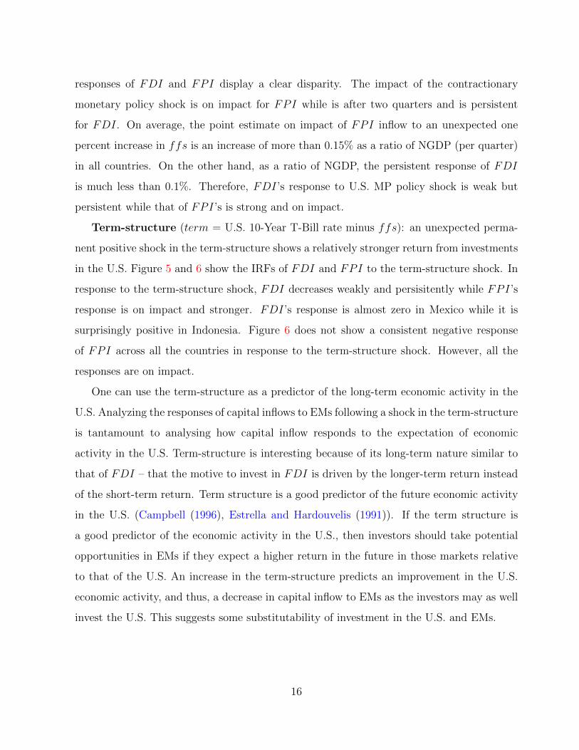
responses of FDI and FPI display a clear disparity. The impact of the contractionary

monetary policy shock is on impact for FPI while is after two quarters and is persistent

for FDI. On average, the point estimate on impact of FPI inflow to an unexpected one

percent increase in ffs is an increase of more than 0.15% as a ratio of NGDP (per quarter)

in all countries. On the other hand, as a ratio of NGDP, the persistent response of FDI

is much less than 0.1%. Therefore, FDI’s response to U.S. MP policy shock is weak but

persistent while that of FPI’s is strong and on impact.

Term-structure (term = U.S. 10-Year T-Bill rate minus ffs): an unexpected perma-

nent positive shock in the term-structure shows a relatively stronger return from investments

in the U.S. Figure 5 and 6 show the IRFs of FDI and FPI to the term-structure shock. In

response to the term-structure shock, FDI decreases weakly and persisitently while FPI’s

response is on impact and stronger. FDI’s response is almost zero in Mexico while it is

surprisingly positive in Indonesia. Figure 6 does not show a consistent negative response

of FPI across all the countries in response to the term-structure shock. However, all the

responses are on impact.

One can use the term-structure as a predictor of the long-term economic activity in the

U.S. Analyzing the responses of capital inflows to EMs following a shock in the term-structure

is tantamount to analysing how capital inflow responds to the expectation of economic

activity in the U.S. Term-structure is interesting because of its long-term nature similar to

that of FDI – that the motive to invest in FDI is driven by the longer-term return instead

of the short-term return. Term structure is a good predictor of the future economic activity

in the U.S. (Campbell (1996), Estrella and Hardouvelis (1991)). If the term structure is

a good predictor of the economic activity in the U.S., then investors should take potential

opportunities in EMs if they expect a higher return in the future in those markets relative

to that of the U.S. An increase in the term-structure predicts an improvement in the U.S.

economic activity, and thus, a decrease in capital inflow to EMs as the investors may as well

invest the U.S. This suggests some substitutability of investment in the U.S. and EMs.

16

Figure 5: FDI IRFs to term shock

−.3

−.2

−.1

0.1

0 4 8 12 16 20

Brazil

−.1

0.1

.20 4 8 12 16 20

India

−.3

−.2

−.1

0.1

0 4 8 12 16 20

Russia

−.1

0.1

.2.3

0 4 8 12 16 20

South Africa

−.06

−.04

−.02

0.0

2.0

4

0 4 8 12 16 20

Mexico

−.2

−.1

0.1

.2.3

0 4 8 12 16 20

Indonesia

−.2

−.15

−.1

−.05

0.0

50 4 8 12 16 20

Philippines

−.2

−.1

0.1

.2

0 4 8 12 16 20

Thailand

Figure 6: FPI IRFs to term shock

−.4

−.3

−.2

−.1

0.1

0 4 8 12 16 20

Brazil

−.4

−.3

−.2

−.1

0.1

0 4 8 12 16 20

India

−.6

−.4

−.2

0.2

.4

0 4 8 12 16 20

Russia

−.3

−.2

−.1

0.1

0 4 8 12 16 20

South Africa

−.05

0.0

5.1

.15

0 4 8 12 16 20

Mexico

−.2

0.2

.4.6

0 4 8 12 16 20

Indonesia

−.2

0.2

.4.6

0 4 8 12 16 20

Philippines

−.8

−.6

−.4

−.2

0.2

0 4 8 12 16 20

Thailand

Notes: Figures 5 and 6 present the IRFs of FDI and FPI to term shock for a recursive VAR(term, y, p, r, e, FDI) and term,FPI, y, p, r, e, FDI) respectively. They are estimated with one standarddeviation bootstrap confidence bands based on 1000 replications, degrees of freedom adjusted, one lag, andtime trend.

As a long-term investment, FDI is sensitive to long-term prospects of the U.S. economic

activity. Its response is persistent though not as strong as FPI’s response. Surprisingly,

17

FPI’s direction of response is positive in Mexico, Indonesia, and Philippines but the response

remains to be on impact and stronger.

In summary, in response an unexpected permanent shock to the U.S. short-term interest

rate (ffs), as the U.S. term-structure decreases, both FDI and FPI increase. FDI’s

response is weak but persistent while that of FPI is stronger and on impact. In response

to an increase in term-structure, FDI decreases weakly but persistently. FPI’s response to

unexpected permanent shock is strong and on impact eventhough it is positive in three of

the countries. These results are consistent with the panel IRFs presented above.

Eventhough the dynamics of the responses to FDI and FPI have not been explored,

some explanations have been provided in the literature about the direction of the responses.

For example, Mody and Taylor (2013) argue that an increase in the U.S. interest rate typically

signals expansionary phase of the U.S. business cycle. This, in turn, creates an environment

in which many investors experience a high degree of exuberance to invest in both the U.S.

and EMs. The high demand for investment and the positive signal of the economic condition

allows investors to take risk in both the U.S. and cross-border countries. On the other hand,

Engel (2014) has pointed that an unexpected increase in the U.S. short-term interest rate

leads to an appreciation of the U.S. dollar and thus a depreciation in the EMs currency

because of exchange rate and interest rate parity. According to Dornbusch (1976), the

monetary contraction in the U.S. leads to a real appreciation of the dollar and the monetary

expansion to depreciation. Thus, an unexpected increase in the U.S. short-term interest rate

makes the purchase of EMs investment cheaper. Furthermore, Calvo et al. (1996) discusses

that a sustained decline in the U.S. interest rate (term-structure) which reached its lowest

level in late 1992 since 1960’s attracted investors to high investment yields in Latin America

and Asia.

4.2.2 The dynamic effects of EMs monetary and exchange rate shocks on FDI

and FPI

In this subsection, I compare and contrast the dynamic and size effects of an unexpected,

permanent, positve shocks to the EMs’ short-term interest rate on FDI and FPI. I then

18

analyze the dynamic and size effects of an unexpected, permanent, positive shocks to the

exchange rate on FDI and FPI. The central result is that while FDIs’ response to the

domestic monetary policy (short-term interest rate) shock and exchange rate shock are weak

(smaller in size) and mostly insignificant, FPIs’ response are stronger (larger in size) and

on impact. Generally, FPI inflow responds positively the monetary policy shock while its

response is negative to the exchange rate shock.

Domestic interest rate (r): Figures 7 and 8 display FDI and FPI IRFs, respectively,

to an unexpected domestic interest rate shock. The impulse responses of FDI are smaller in

size and insignificant in most of the countries while they are positive in India, Indonesia, and

Thailand in the span of a year. In contrast, the responses are stronger for FPI. Particularly

in Brazil, the Philippines, and Thailand FPI’s responses are significantly large and positive.

The on impact median impulse responses of FPI are generally positive though not significant

in most of the countries while they are negative in Russia and Indonesia. Therefore, FPI

inflow generally increase as the domestic interest rate increases while it is not necessarily the

case for FDI inflow.

As the domestic short-term interest rate rises, EMs’ domestic investors cost of borrowing

relative to that of foreign investors increases, which in turn makes it cheaper for foreign

investors to invest in EMs assets. However, this relationship is not straightforward. An

increased real interest rate (rate of return on investment in EMs) may cause capital inflow

slow down because it may signal an increase in expected default rates (Calvo, 1998). In

other words, as Stiglitz and Weiss (1981) put it, borrowers offering to pay high rates may

signal that they are the least creditworthy.

19

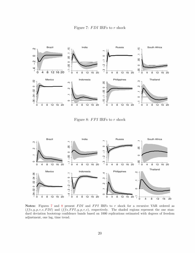
Figure 7: FDI IRFs to r shock

−.4

−.2

0.2

0 4 8 12 16 20

Brazil

−.1

−.05

0.0

5.1

.15

0 4 8 12 16 20

India

−.3

−.2

−.1

0.1

0 4 8 12 16 20

Russia

−.05

0.0

5.1

.15

0 4 8 12 16 20

South Africa

−.06

−.04

−.02

0.0

2

0 4 8 12 16 20

Mexico

0.1

.2.3

0 4 8 12 16 20

Indonesia

−.15

−.1

−.05

0.0

50 4 8 12 16 20

Philippines

−.1

0.1

.2.3

0 4 8 12 16 20

Thailand

Figure 8: FPI IRFs to r shock

0.1

.2.3

0 4 8 12 16 20

Brazil

−.1

−.05

0.0

5.1

0 4 8 12 16 20

India

−.3

−.2

−.1

0.1

0 4 8 12 16 20

Russia−.

050

.05

.1

0 4 8 12 16 20

South Africa

−.04

−.02

0.0

2.0

4.0

6

0 4 8 12 16 20

Mexico

−.4

−.3

−.2

−.1

0.1

0 4 8 12 16 20

Indonesia

0.1

.2.3

.4

0 4 8 12 16 20

Philippines

−.1

0.1

.2

0 4 8 12 16 20

Thailand

Notes: Figures 7 and 8 present FDI and FPI IRFs to r shock for a recursive VAR ordered as(ffs, y, p, r, e, FDI) and (ffs, FPI, y, p, r, e), respectively. The shaded regions represent the one stan-dard deviation bootstrap confidence bands based on 1000 replications estimated with degrees of freedomadjustment, one lag, time trend.

20

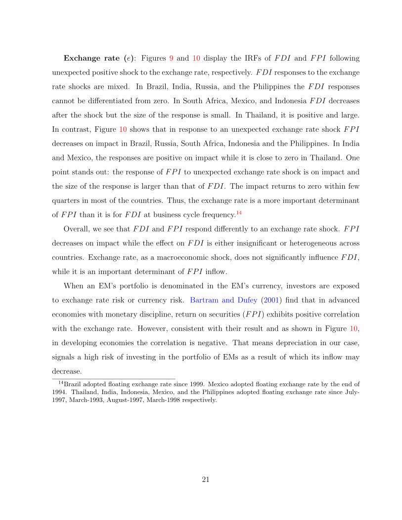
Exchange rate (e): Figures 9 and 10 display the IRFs of FDI and FPI following

unexpected positive shock to the exchange rate, respectively. FDI responses to the exchange

rate shocks are mixed. In Brazil, India, Russia, and the Philippines the FDI responses

cannot be differentiated from zero. In South Africa, Mexico, and Indonesia FDI decreases

after the shock but the size of the response is small. In Thailand, it is positive and large.

In contrast, Figure 10 shows that in response to an unexpected exchange rate shock FPI

decreases on impact in Brazil, Russia, South Africa, Indonesia and the Philippines. In India

and Mexico, the responses are positive on impact while it is close to zero in Thailand. One

point stands out: the response of FPI to unexpected exchange rate shock is on impact and

the size of the response is larger than that of FDI. The impact returns to zero within few

quarters in most of the countries. Thus, the exchange rate is a more important determinant

of FPI than it is for FDI at business cycle frequency.14

Overall, we see that FDI and FPI respond differently to an exchange rate shock. FPI

decreases on impact while the effect on FDI is either insignificant or heterogeneous across

countries. Exchange rate, as a macroeconomic shock, does not significantly influence FDI,

while it is an important determinant of FPI inflow.

When an EM’s portfolio is denominated in the EM’s currency, investors are exposed

to exchange rate risk or currency risk. Bartram and Dufey (2001) find that in advanced

economies with monetary discipline, return on securities (FPI) exhibits positive correlation

with the exchange rate. However, consistent with their result and as shown in Figure 10,

in developing economies the correlation is negative. That means depreciation in our case,

signals a high risk of investing in the portfolio of EMs as a result of which its inflow may

decrease.

14Brazil adopted floating exchange rate since 1999. Mexico adopted floating exchange rate by the end of1994. Thailand, India, Indonesia, Mexico, and the Philippines adopted floating exchange rate since July-1997, March-1993, August-1997, March-1998 respectively.

21

Figure 9: FDI IRFs to e shock

−.4

−.2

0.2

.4

0 4 8 12 16 20

Brazil

−.05

0.0

5.1

0 4 8 12 16 20

India

−.3

−.2

−.1

0.1

0 4 8 12 16 20

Russia

−.15

−.1

−.05

0.0

5

0 4 8 12 16 20

South Africa

−.08

−.06

−.04

−.02

0

0 4 8 12 16 20

Mexico

−.8

−.6

−.4

−.2

0

0 4 8 12 16 20

Indonesia

−.3

−.2

−.1

0.1

0 4 8 12 16 20

Philippines

0.1

.2.3

.4

0 4 8 12 16 20

Thailand

Figure 10: FPI IRFs to e shock

−.15

−.1

−.05

0.0

5

0 4 8 12 16 20

Brazil

0.1

.2.3

0 4 8 12 16 20

India

−.4

−.3

−.2

−.1

0.1

0 4 8 12 16 20

Russia−.

1−.

050

.05

0 4 8 12 16 20

South Africa

−.05

0.0

5.1

.15

0 4 8 12 16 20

Mexico

−.2

−.1

0.1

.2.3

0 4 8 12 16 20

Indonesia

−.2

−.15

−.1

−.05

0.0

5

0 4 8 12 16 20

Philippines

−.1

−.05

0.0

5.1

.15

0 4 8 12 16 20

Thailand

Notes: Figures 7 and 8 present FDI and FPI IRFs to e shock for a recursive VAR ordered as(ffs, y, p, r, e, FDI) and (ffs, FPI, y, p, r, e), respectively. The shaded regions represent the one stan-dard deviation bootstrap confidence bands based on 1000 replications estimated with degrees of freedomadjustment, one lag, time trend.

22

There is no consensus either in theory or empirical studies about the effect of exchange

rate on FDI. One possible reason for the disagreement is that the impact of exchange rate on

FDI is different across industries. The effect of an exchange rate shock depends on whether

the motive of the FDI inflow is to gain market access in EMs or to reduce production

costs. Besides, whether a firm exports its product or imports its factors of production

determines the effect of exchange rate on FDI expansion or contraction. In other words, an

appreciation may increase profits through cheaper imported inputs or it may reduce profits

through lower export receipts (Buch and Kleinert (2008)). Thus, the heterogeneous FDI

IRFs across countries for after an unexpected shock to the exchange rate shown in Figure 9

is not surprising.

In summary of this subsection, I find that domestic monetary and exchange rate shocks

have less impact on FDI. In contrast, FPI’s response to domestic monetary and exchange

rate shocks are on impact and are larger in size. Forbes and Warnock (2012) argue that

domestic macroeconomic characteristics are less important in determining foreign capital

inflows. Considering the dynamics, sizes, and composition of flows, the results of this paper

is consistent with their findings in the case FDI but fails to share their conclusion in the

case of FPI.

4.2.3 The dynamic effects of EMs’ output and price level shocks on FDI and

FPI

In this subsection, I analyze the impulse responses of FDI and FPI to domestic output

and price shocks. I use domestic industrial production index for output and the EMs’

consumer price index for the domestic price. I compare and contrast FDI and FPI IRFs

to an unexpected positive shocks to the industrial production and the EMs consumer price

indices.

Domestic industrial production index (y): Figures 11 and 12 show the IRFs of

FDI and FPI respectively after an unexpected shock to y. In Figure 11, FDI’s response

to y is mixed. It responds positively in Russia, Indonesia, and Thailand while it is negative

in Brazil and south Africa. In India, Mexico, and Philippines, FDI’s responses to y shock

23

cannot be differentiated from zero. In contrast, the on impact strong response of FPI to y

shock is clear. However, in Figure 12, the direction of the responses are also mixed in the

case of FPI.

Figure 11: FDI IRFs to y shock

−.3

−.2

−.1

0.1

0 4 8 12 16 20

Brazil−.

1−.

050

.05

.1

0 4 8 12 16 20

India

−.1

0.1

.2.3

.4

0 4 8 12 16 20

Russia

−.15

−.1

−.05

0.0

5

0 4 8 12 16 20

South Africa

−.04

−.02

0.0

2

0 4 8 12 16 20

Mexico

−.1

0.1

.2.3

0 4 8 12 16 20

Indonesia

−.2

−.1

0.1

0 4 8 12 16 20

Philippines

−.2

0.2

.4.6

.8

0 4 8 12 16 20

Thailand

Figure 12: FPI IRFs to y shock

−.3

−.2

−.1

0.1

0 4 8 12 16 20

Brazil

−.1

0.1

.2.3

0 4 8 12 16 20

India

−.1

0.1

.2.3

.4

0 4 8 12 16 20

Russia

−.08

−.06

−.04

−.02

0.0

2

0 4 8 12 16 20

South Africa

−.08

−.06

−.04

−.02

0

0 4 8 12 16 20

Mexico

−.4

−.3

−.2

−.1

0.1

0 4 8 12 16 20

Indonesia

−.4

−.3

−.2

−.1

0

0 4 8 12 16 20

Philippines

−.1

0.1

.2

0 4 8 12 16 20

Notes: Figures 11 and 12 present FDI and FPI IRFs to y shock for a recursive VAR ordered as(ffs, y, p, r, e, FDI) and (ffs, FPI, y, p, r, e), respectively. The shaded regions represent the one stan-dard deviation bootstrap confidence bands based on 1000 replications estimated with degrees of freedomadjustment, one lag, time trend.

24

FPI response is stronger and on impact relative to FDI’s. A positive or negative

response of capital inflow’s in response to an expanding domestic economy has been docu-

mented in the literature. From the standard endowment model of the small open economy,

because households smooth consumption, saving is procyclical. Therefore, capital inflows

– borrowing from abroad, can be countercyclical. However, if the economy borrows during

good times, as shown by Calvo et al. (1994) in the case of EMs, capital inflow can be pro-

cyclical and thus have a positive correlation with industrial production index. Furthermore,

foreign investors respond to improving domestic economies of EMs and thus capital inflow

can increase.15

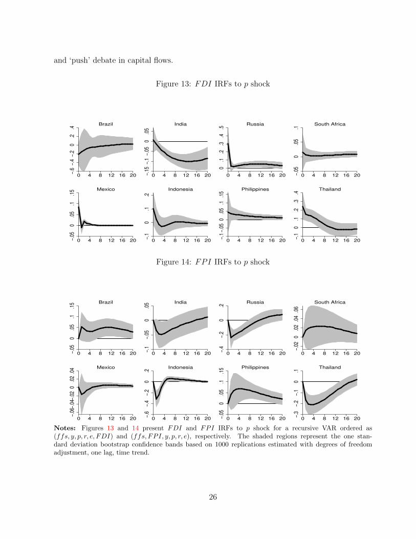
Domestic price level (p): Figure 13 and 14 show the responses of FDI and FPI in-

flows to a positive domestic price shock, respectively. FDI’s response to the consumer price

index shock cannot be differentiated from zero in Brazil, South Africa, Indonesia and the

Philippines. For FPI the responses are negative in India, Russia, Indonesia, and Thailand

while they cannot be differentiated zero in Brazil, South Africa, and Mexico. In the Philip-

pines, the responses are positive. In general, FPI’s response is relatively stronger and on

impact while the direction (sign) of the responses are mixed and weaker for both FDI and

FPI. For net portfolio inflows, Fratzscher (2012) finds that the effect of domestic consumer

price index was minimal for the short period before the financial crisis.

In summary, results from panel and country-specific SVARs presented is an improvement

to the literature in terms of dynamics, size, and composition of gross capital inflows to EMs.

The results can be summarizes as: 1) in response to an unexpected positive shock to the

U.S. federal fund’s shadow rate, as the term-structure in the U.S. decreases, FDI gross

inflows to the EMs increases and the increase is persistent while the increase in FPI inflows

is relatively stronger and is on impact; 2) domestic monetary and exchange rate shocks have

less impact on FDI while FPI’s response to domestic monetary and exchange rate shocks

are on impact and are larger in size; 3) in response to shocks to the industrial production

and the consumer price indices, the directions (signs) of both FDI and FPI inflows are

mixed and inconsistent across countries. In the next section, I analyze the dynamic ‘pull’

15For more explanation see Calvo et al. (1993), Calvo et al. (1994), and Calvo and Vegh (1999).

25

and ‘push’ debate in capital flows.

Figure 13: FDI IRFs to p shock

−.6

−.4

−.2

0.2

.4

0 4 8 12 16 20

Brazil

−.15

−.1

−.05

0.0

5

0 4 8 12 16 20

India

0.1

.2.3

.4.5

0 4 8 12 16 20

Russia

−.05

0.0

5.1

0 4 8 12 16 20

South Africa

−.05

0.0

5.1

.15

0 4 8 12 16 20

Mexico

−.1

0.1

.2

0 4 8 12 16 20

Indonesia

−.1

−.05

0.0

5.1

.15

0 4 8 12 16 20

Philippines

−.1

0.1

.2.3

.4

0 4 8 12 16 20

Thailand

Figure 14: FPI IRFs to p shock

−.05

0.0

5.1

.15

0 4 8 12 16 20

Brazil

−.1

−.05

0.0

5

0 4 8 12 16 20

India

−.4

−.2

0.2

0 4 8 12 16 20

Russia

−.02

0.0

2.0

4.0

6

0 4 8 12 16 20

South Africa

−.06

−.04

−.02

0.0

2.0

4

0 4 8 12 16 20

Mexico

−.6

−.4

−.2

0.2

0 4 8 12 16 20

Indonesia

−.05

0.0

5.1

.15

0 4 8 12 16 20

Philippines

−.3

−.2

−.1

0.1

0 4 8 12 16 20

Thailand

Notes: Figures 13 and 14 present FDI and FPI IRFs to p shock for a recursive VAR ordered as(ffs, y, p, r, e, FDI) and (ffs, FPI, y, p, r, e), respectively. The shaded regions represent the one stan-dard deviation bootstrap confidence bands based on 1000 replications estimated with degrees of freedomadjustment, one lag, time trend.

26

4.3 The ‘pull’ and ‘push’ debate in capital flows

Global factors are push factors that influence capital flows to EMs’ while EMs economic

environment has a pulling effect on capital flows. Some research emphasizes common global

external shocks in explaining capital flows; others underline country-specific macroeconomic

policies, institutions, and risk. If the common external shocks explain the dynamics of capital

flows, then the implication is that countries cannot shield themselves from these shocks.

The opposite argument is that, because capital flows are heterogeneous across countries (for

example, lesser inflows in Sub-Saharan Africa), then it is the country-specific factors that

explain capital flows to those countries. This debate remains unresolved.

This paper attempts to quantify the dynamics and sizes of contributions of global (push)

and domestic (pull) shocks on the composition of inflows to examine the relative importance

of each factor for each country. Therefore, I analyze the quantitative contributions of the

factors in influencing categories of capital inflows using structural forecast-error variance

decomposition (FEVD) after the SVAR estimations. The important implication of using

SVAR is that we can quantify and rank the percentage contribution of push versus pull

factors to the dynamics and variations in capital flows. Unlike SVARs, this is generally

not available for panel data regressions. That is, even though FDI inflow is not strongly

responsive to domestic macroeconomic conditions, we can still quantify what percentage of

its dynamics can be explained by the push and pull factors.

Figures 15 and 16 show the FEVD for FDI and FPI inflows, respectively. On the

vertical axis (y-axis), I denote the percentage contribution of each variable to the variation

in each inflow category. On the horizontal axis (x-axis), the 20 quarters after the shock

are denoted. Each graph shows the percentage contribution of the variable at the specific

quarter. For example, approximately 7% of the variation in FDI in South Africa is explained

by the U.S. short-term interest rate (ffs). Domestic industrial production (y) is ranked in

the top three of the ranking order in explaining the variation in FDI in Brazil, Russia, and

Thailand. Exchange rate (e) explains large variation in FDI in Indonesia and Thailand.

Despite the variations across the countries, ffs is not the most important variable across all

27

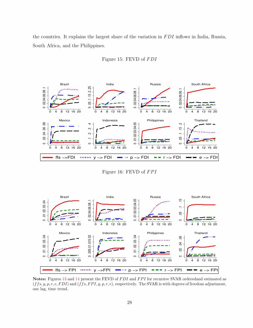
the countries. It explains the largest share of the variation in FDI inflows in India, Russia,

South Africa, and the Philippines.

Figure 15: FEVD of FDI

0.0

2.04

.06.

08.1

0 4 8 12 16 20

Brazil

0.0

5.1

.15

.2.2

5

0 4 8 12 16 20

India

0.0

2.04

.06.

08.1

0 4 8 12 16 20

Russia

0.0

2.04

.06.

08.1

0 4 8 12 16 20

South Africa

0.0

2.0

4.0

6.0

8

0 4 8 12 16 20

Mexico

0.1

.2.3

.4

0 4 8 12 16 20

Indonesia

0.0

1.02

.03.

04.0

5

0 4 8 12 16 20

Philippines

0.0

5.1

.15

.2

0 4 8 12 16 20

Thailand

ffs −>FDI y −> FDI p −> FDI r −> FDI e −> FDI

Figure 16: FEVD of FPI

0.0

1.0

2.0

3.0

4

0 4 8 12 16 20

Brazil

0.0

2.04

.06.

08.1

0 4 8 12 16 20

India

0.0

1.02

.03.

04.0

5

0 4 8 12 16 20

Russia

0.0

5.1

.15

0 4 8 12 16 20

South Africa

0.0

1.0

2.0

3.0

4

0 4 8 12 16 20

Mexico

0.0

05.0

1.0

15.0

2

0 4 8 12 16 20

Indonesia

0.0

1.0

2.0

3.0

4

0 4 8 12 16 20

Philippines

0.0

2.0

4.0

6

0 4 8 12 16 20

Thailand

ffs −> FPI y −>FPI p −> FPI r −> FPI e −> FPI

Notes: Figures 13 and 14 present the FEVD of FDI and FPI for recursive SVAR orderedand estimated as(ffs, y, p, r, e, FDI) and (ffs, FPI, y, p, r, e), respectively. The SVAR is with degrees of freedom adjustment,one lag, time trend.

28

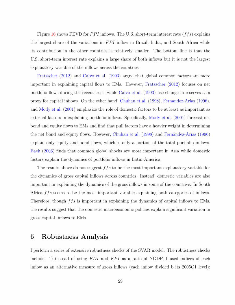
Figure 16 shows FEVD for FPI inflows. The U.S. short-term interest rate (ffs) explains

the largest share of the variations in FPI inflow in Brazil, India, and South Africa while

its contribution in the other countries is relatively smaller. The bottom line is that the

U.S. short-term interest rate explains a large share of both inflows but it is not the largest

explanatory variable of the inflows across the countries.

Fratzscher (2012) and Calvo et al. (1993) argue that global common factors are more

important in explaining capital flows to EMs. However, Fratzscher (2012) focuses on net

portfolio flows during the recent crisis while Calvo et al. (1993) use change in reserves as a

proxy for capital inflows. On the other hand, Chuhan et al. (1998), Fernandez-Arias (1996),

and Mody et al. (2001) emphasize the role of domestic factors to be at least as important as

external factors in explaining portfolio inflows. Specifically, Mody et al. (2001) forecast net

bond and equity flows to EMs and find that pull factors have a heavier weight in determining

the net bond and equity flows. However, Chuhan et al. (1998) and Fernandez-Arias (1996)

explain only equity and bond flows, which is only a portion of the total portfolio inflows.

Baek (2006) finds that common global shocks are more important in Asia while domestic

factors explain the dynamics of portfolio inflows in Latin America.

The results above do not suggest ffs to be the most important explanatory variable for

the dynamics of gross capital inflows across countries. Instead, domestic variables are also

important in explaining the dynamics of the gross inflows in some of the countries. In South

Africa ffs seems to be the most important variable explaining both categories of inflows.

Therefore, though ffs is important in explaining the dynamics of capital inflows to EMs,

the results suggest that the domestic macroeconomic policies explain significant variation in

gross capital inflows to EMs.

5 Robustness Analysis

I perform a series of extensive robustness checks of the SVAR model. The robustness checks

include: 1) instead of using FDI and FPI as a ratio of NGDP, I used indices of each

inflow as an alternative measure of gross inflows (each inflow divided b its 2005Q1 level);

29

2) various alternate orderings; 3) using only the data up to 2008Q3; and 4) the inclusion of

U.S. industrial production index in the model.16

First, I used the indices of FDI and FPI using 2005Q1 as a base quarter and checked

the results. The results are qualitatively unchanged whether the index of FDI and FPI,

instead of using the respective inflow as a ratio of NGDP is used. This is a new robustness

checking alternative that this paper introduces.

I examined the sensitivity of the result to various alternative orderings of the variables.

A caveat here is that I can not alter the position of U.S. interest rate variables because of

the small open economy assumption. Altering the position of U.S. interest rate variables is

tantamount to assuming that they are influenced by EMs macroeconomic variables. How-

ever, the alternative orderings, leaving the first variable in the order (U.S. interest rate or

term-structure) in its position, were used to check whether the results stand that scrutiny.

From that exercise, the results presented continue to hold. I have provided an online ap-

pendix for the results of a recursive estimation in which I used (ffs, FDI, y, p, r, e,) and

(ffs, y, p, r, e, FPI,), for FDI and FPI respectively.

At the beginning of this project, I started including the U.S. industrial production index

as the second element in the ordering of the SVAR. However, focusing on the effect of the U.S.

MP on capital inflows to the EMs, I dropped the U.S. industrial production. The results are

not altered by the inclusion or dropping of the U.S. industrial production index. I followed

Bruno and Shin (2015) that also used U.S. industrial production index for robustness check.

In summary, the results in this paper are robust to using indices of FDI and FPI,

using data up to 2008Q3, various alternate orderings, and the inclusion of U.S. industrial

production index in the model.

16To save space, the robustness analyses results using the indices of the inflows and an alternative orderingof the variables in a recursive VAR are provided in the online appendix.

30

6 Concluding Remarks

This paper examines the dynamic effects of the U.S. conventional monetary policy shocks as

well as the domestic monetary and exchange rate shocks on gross categories capital inflows to

emerging markets. The U.S. federal fund’s shadow rate and the U.S. term-structure are used

as a proxy for advanced economies’ monetary policy stance. The paper explicitly compares

FDI and FPI responses to the U.S. federal fund’s shadow rate, emerging markets’ interest

rates and exchange rates empirically using panel and country-specific structural vector auto-

regressions. It also quantifies and compares the relative contributions of the “push” versus

“pull” factors.

The results show that FDI inflows decrease persistently but weakly in response to un-

expected increase in the spread between the U.S. 10-Year and federal funds rate (term-

structure) while the response of FPI to the same shock is stronger and on impact. Gross

FPI inflows to emerging markets increase on impact as the U.S. federal fund’s shadow rate

increases or as the term-structure in the U.S. decreases. FPI inflows are strongly responsive

to the macroeconomic shocks of emerging markets in the first few quarters after a shock

while the response of FDI is weaker. These results are consistent with the arguments in

the literature that foreign direct inflow is weakly sensitive to macroeconomic variables. The

suggested implication of these results is that macro-prudential and capital control policies of

emerging markets are more effective when directed at portfolio inflows. Using forecast-error

variance decomposition, the paper compares the contributions of the U.S. monetary policy

with domestic macroeconomic shocks to the dynamics of both gross capital inflow types.

Although the U.S. monetary policy explains a significant percentage of the variation in each

category of gross inflow, the results do not suggest the dominance of the “push” over “pull”

factors in either type of inflow or across the emerging market countries.

The conclusions suggest that a unifying theory of capital flow categories that takes into

account the business cycle and monetary policies of both advanced economies and emerging

markets may be necessary. Particularly, developing theoretical models which capture the

differences in the characteristics of FPI and FDI is important.

31

References

Adelman, Jeremy (1998), “Tequila hangover: Latin america’s debt crisis.” Studies in PoliticalEconomy, 55.

Aguiar, Mark and Gita Gopinath (2007), “Emerging market business cycles: The cycle isthe trend.” Journal of political Economy, 115, 69–102.

Ahlquist, John S (2006), “Economic policy, institutions, and capital flows: Portfolio anddirect investment flows in developing countries.” International Studies Quarterly, 50, 681–704.

Ahmed, Shaghil and Andrei Zlate (2014), “Capital flows to emerging market economies: Abrave new world?” Journal of International Money and Finance, 48, 221–248.

Alejandro, Carlos F Diaz (1983), “Stories of the 1930s for the 1980s.” In Financial policiesand the world capital market: The problem of Latin American countries, 5–40, Universityof Chicago Press.

Baek, In-Mee (2006), “Portfolio investment flows to Asia and Latin America: Pull, push ormarket sentiment?” Journal of Asian Economics, 17, 363–373.

Bakardzhieva, Damyana, Sami Ben Naceur, and Bassem Kamar (2010), “The impact ofcapital and foreign exchange flows on the competitiveness of developing countries.” IMFWorking Papers, 1–30.

Barassi, Marco R, Guglielmo Maria Caporale, and Stephen G Hall (2001), “Irreducibilityand structural cointegrating relations: An application to the G-7 long-term interest rates.”International Journal of Finance & Economics, 6, 127–138.

Barkoulas, John T, Christopher F Baum, and Gurkan S Oguz (1997), “Fractional dynamicsin a system of long term international interest rates.” International Journal of Finance,9, 586–606.

Bartram, Sohnke M and Gunter Dufey (2001), “International portfolio investment: Theory,evidence, and institutional framework.” Financial Markets, Institutions & Instruments,10, 85–155.

Brooks, Robin, Hali Edison, Manmohan S Kumar, and Torsten Sløk (2004), “Exchange ratesand capital flows.” European Financial Management, 10, 511–533.

Bruno, Valentina and Hyun Song Shin (2015), “Capital flows and the risk-taking channel ofmonetary policy.” Journal of Monetary Economics, 71, 119–132.

Buch, Claudia M and Jorn Kleinert (2008), “Exchange rates and FDI: Goods versus capitalmarket frictions.” The World Economy, 31, 1185–1207.

32

Calvo, Guillermo A (1998), “Capital flows and capital-market crises: The simple economicsof sudden stops.” Journal of Applied Economics, 1, 35–54.

Calvo, Guillermo A, Leonardo Leiderman, and Carmen M Reinhart (1993), “Capital inflowsand real exchange rate appreciation in Latin America: The role of external factors.” StaffPapers-International Monetary Fund, 108–151.

Calvo, Guillermo A, Leonardo Leiderman, and Carmen M Reinhart (1994), “The capitalinflows problem: Concepts and issues.” Contemporary Economic Policy, 12, 54–66.

Calvo, Guillermo A, Leonardo Leiderman, and Carmen M Reinhart (1996), “Inflows ofcapital to developing countries in the 1990s.” The Journal of Economic Perspectives, 123–139.

Calvo, Guillermo A and Carlos A Vegh (1999), “Inflation stabilization and BOP crises indeveloping countries.” Handbook of macroeconomics, 1, 1531–1614.

Campbell, John Y (1996), “Understanding risk and return.” Journal of Political Economy,298–345.

Christiano, Lawrence J, Martin Eichenbaum, and Charles L Evans (1999), “Monetary policyshocks: What have we learned and to what end?” Handbook of macroeconomics, 1, 65–148.

Chuhan, Punam, Stijn Claessens, and Nlandu Mamingi (1998), “Equity and bond flows toLatin America and Asia: The role of global and country factors.” Journal of DevelopmentEconomics, 55, 439–463.

Dornbusch, Rudiger (1976), “Expectations and exchange rate dynamics.” The Journal ofPolitical Economy, 1161–1176.

Eichanbaum, E and LE Charles (1995), “Some empirical evidence on the effects of shocksto monetary policy on exchange rate.” The Quarterly Journal of Economics, 975–1009.

Eichengreen, Barry (1990), “Trends and cycles in foreign lending.” Technical Report No.w3411, National Bureau of Economic Research.

Engel, Charles (2014), “Exchange rates and interest parity.” Handbook of International Eco-nomics, 4, 453.

Estrella, Arturo and Gikas A Hardouvelis (1991), “The term structure as a predictor of realeconomic activity.” The Journal of Finance, 46, 555–576.

Fernandez-Arias, Eduardo (1996), “The new wave of private capital inflows: push or pull?”Journal of development economics, 48, 389–418.

33

Fernandez-Villaverde, Jesus, Grey Gordon, Pablo Guerron-Quintana, and Juan F Rubio-Ramirez (2015), “Nonlinear adventures at the zero lower bound.” Journal of EconomicDynamics and Control, 57, 182–204.

Forbes, Kristin J and Francis E Warnock (2012), “Capital flow waves: Surges, stops, flight,and retrenchment.” Journal of International Economics, 88, 235–251.

Fratzscher, Marcel (2012), “Capital flows, push versus pull factors and the global financialcrisis.” Journal of International Economics, 88, 341–356.

Gertler, Mark and Peter Karadi (2015), “Monetary policy surprises, credit costs, and eco-nomic activity.” American Economic Journal: Macroeconomics, 7, 44–76.

Gourinchas, Pierre-Olivier and Olivier Jeanne (2013), “Capital flows to developing countries:The allocation puzzle.” The Review of Economic Studies, rdt004.

Gourinchas, Pierre-Olivier and Helene Rey (2013), “External adjustment, global imbalancesand valuation effects.” Technical Report No. w19240, National Bureau of Economic Re-search.

Gruber, Joseph and Steven Kamin (2009), “Do differences in financial development explainthe global pattern of current account imbalances?” Review of International Economics,17, 667–688.

Hamilton, James Douglas (1994), Time series analysis, volume 2. Princeton university pressPrinceton.

Janus, Thorsten and Daniel Riera-Crichton (2013), “International gross capital flows: Newuses of balance of payments data and application to financial crises.” Journal of PolicyModeling, 35, 16–28.

Kilian, Lutz (2013), “Structural vector autoregressions.” Technical report, Edward ElgarPublishing.

Kiran, Burcu (2012), “Integration of long-term interest rates: Empirical evidence for G7countries.” Global Economic Review, 41, 279–290.

Lane, Philip R and Gian Maria Milesi-Ferretti (2007), “The external wealth of nations markII: Revised and extended estimates of foreign assets and liabilities, 1970–2004.” Journalof international Economics, 73, 223–250.

Lim, Jamus Jerome, Sanket Mohapatra, and Marc Tinker Stocker (2014), “Taper, QE, bye?The effect of quantitative easing on financial flows to developing countries.” World BankPolicy Research Working Paper. Available at SSRN: http://ssrn.com/abstract=2417518.

Liu, Zheng, Daniel F Waggoner, and Tao Zha (2011), “Sources of macroeconomic fluctua-tions: A regime-switching DSGE approach.” Quantitative Economics, 2, 251–301.

34

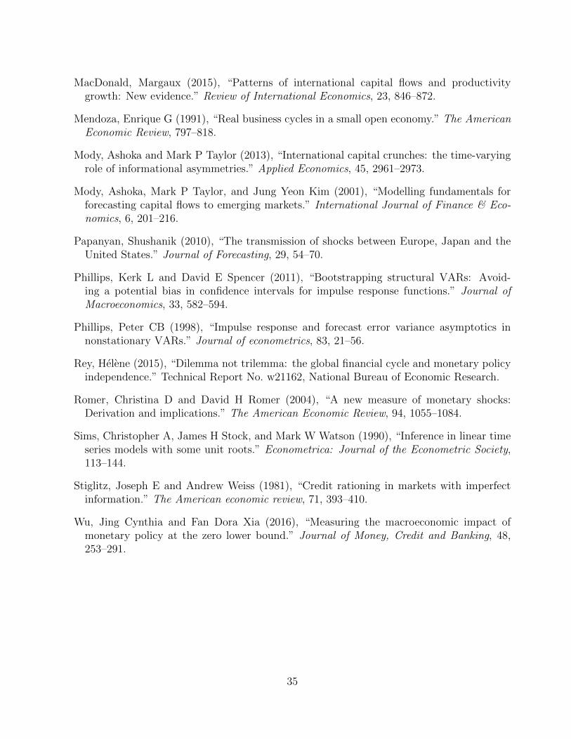
MacDonald, Margaux (2015), “Patterns of international capital flows and productivitygrowth: New evidence.” Review of International Economics, 23, 846–872.

Mendoza, Enrique G (1991), “Real business cycles in a small open economy.” The AmericanEconomic Review, 797–818.

Mody, Ashoka and Mark P Taylor (2013), “International capital crunches: the time-varyingrole of informational asymmetries.” Applied Economics, 45, 2961–2973.

Mody, Ashoka, Mark P Taylor, and Jung Yeon Kim (2001), “Modelling fundamentals forforecasting capital flows to emerging markets.” International Journal of Finance & Eco-nomics, 6, 201–216.

Papanyan, Shushanik (2010), “The transmission of shocks between Europe, Japan and theUnited States.” Journal of Forecasting, 29, 54–70.

Phillips, Kerk L and David E Spencer (2011), “Bootstrapping structural VARs: Avoid-ing a potential bias in confidence intervals for impulse response functions.” Journal ofMacroeconomics, 33, 582–594.

Phillips, Peter CB (1998), “Impulse response and forecast error variance asymptotics innonstationary VARs.” Journal of econometrics, 83, 21–56.

Rey, Helene (2015), “Dilemma not trilemma: the global financial cycle and monetary policyindependence.” Technical Report No. w21162, National Bureau of Economic Research.

Romer, Christina D and David H Romer (2004), “A new measure of monetary shocks:Derivation and implications.” The American Economic Review, 94, 1055–1084.

Sims, Christopher A, James H Stock, and Mark W Watson (1990), “Inference in linear timeseries models with some unit roots.” Econometrica: Journal of the Econometric Society,113–144.

Stiglitz, Joseph E and Andrew Weiss (1981), “Credit rationing in markets with imperfectinformation.” The American economic review, 71, 393–410.

Wu, Jing Cynthia and Fan Dora Xia (2016), “Measuring the macroeconomic impact ofmonetary policy at the zero lower bound.” Journal of Money, Credit and Banking, 48,253–291.

35

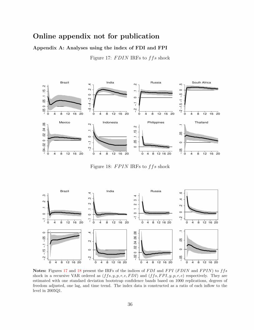
Online appendix not for publication

Appendix A: Analyses using the index of FDI and FPI

Figure 17: FDIN IRFs to ffs shock

−.05

0.0

5.1

.15

.2

0 4 8 12 16 20

Brazil

−.6

−.4

−.2

0.2

.4

0 4 8 12 16 20

India

−.2

−.1

0.1

.2

0 4 8 12 16 20

Russia

−2−1

.5−1

−.5

0.5

0 4 8 12 16 20

South Africa

−.04

−.02

0.0

2.0

4.0

6

0 4 8 12 16 20

Mexico

−.2

−.1

0.1

.2

0 4 8 12 16 20

Indonesia

0.0

5.1

.15

.2

0 4 8 12 16 20

Philippines

−.05

0.0

5.1

0 4 8 12 16 20

Thailand

Figure 18: FPIN IRFs to ffs shock

−.1

0.1

.2.3

0 4 8 12 16 20

Brazil

−.1

0.1

.2.3

.4

0 4 8 12 16 20

India

−1

01

23

4

0 4 8 12 16 20

Russia

−.2

0.2

.4.6

0 4 8 12 16 20

−.2

−.1

5−

.1−

.05

0

0 4 8 12 16 20

−.2

0.2

.4

0 4 8 12 16 20

−.0

20

.02

.04

.06

.08

0 4 8 12 16 20

−.0

50

.05

.1

0 4 8 12 16 20

Notes: Figures 17 and 18 present the IRFs of the indices of FDI and FPI (FDIN and FPIN) to ffsshock in a recursive VAR ordered as (ffs, y, p, r, e, FDI) and (ffs, FPI, y, p, r, e) respectively. They areestimated with one standard deviation bootstrap confidence bands based on 1000 replications, degrees offreedom adjusted, one lag, and time trend. The index data is constructed as a ratio of each inflow to thelevel in 2005Q1.

36

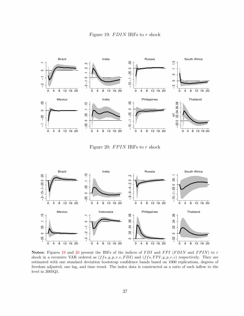
Figure 19: FDIN IRFs to r shock

−.2

−.1

0.1

0 4 8 12 16 20

Brazil

−.2

−.1

0.1

.2.3

0 4 8 12 16 20

India

−.15

−.1

−.05

0.0

5

0 4 8 12 16 20

Russia

−.5

0.5

11.

5

0 4 8 12 16 20

South Africa

−.1

−.05

0.0

5

0 4 8 12 16 20

Mexico

−.05

0.0

5.1

.15

0 4 8 12 16 20

India

−.15

−.1

−.05

0.0

50 4 8 12 16 20

Philippines

−.02

0.0

2.0

4.0

6.0

8si

rf

0 4 8 12 16 20

Thailand

Figure 20: FPIN IRFs to r shock

−.2−

.15−

.1−.

050

.05

0 4 8 12 16 20

Brazil

−.05

0.0

5.1

.15

0 4 8 12 16 20

India

−.8

−.6

−.4

−.2

0.2

0 4 8 12 16 20

Russia−.

15−.

1−.

050

.05

.1

0 4 8 12 16 20

South Africa

−.05

0.0

5.1

.15

0 4 8 12 16 20

Mexico

−.3

−.2

−.1

0.1

0 4 8 12 16 20

Indonesia

0.0

2.0

4.0

6.0

8

0 4 8 12 16 20

Philippines

−.02

0.0

2.0

4.0

6

0 4 8 12 16 20

Thailand

Notes: Figures 19 and 20 present the IRFs of the indices of FDI and FPI (FDIN and FPIN) to rshock in a recursive VAR ordered as (ffs, y, p, r, e, FDI) and (ffs, FPI, y, p, r, e) respectively. They areestimated with one standard deviation bootstrap confidence bands based on 1000 replications, degrees offreedom adjusted, one lag, and time trend. The index data is constructed as a ratio of each inflow to thelevel in 2005Q1.

37

Figure 21: FDIN IRFs to e shock

−.2−

.15−

.1−.

050

.05

0 4 8 12 16 20

Brazil

−.2

−.1

0.1

.2

0 4 8 12 16 20

India

−.15

−.1

−.05

0.0

5

0 4 8 12 16 20

Russia

−2−1

.5−1

−.5

0.5

sirf

0 4 8 12 16 20

South Africa

−.15

−.1

−.05

0

0 4 8 12 16 20

Mexico

−.4

−.3

−.2

−.1

0.1

0 4 8 12 16 20

Indonesia

−.15

−.1

−.05

00 4 8 12 16 20

Philippines

0.0

5.1

.15

0 4 8 12 16 20

Thailand

Figure 22: FPIN IRFs to e shock

−.15

−.1

−.05

0

0 4 8 12 16 20

Brazil

0.0

5.1

.15

.2

0 4 8 12 16 20

India

−.8

−.6

−.4

−.2

0.2

0 4 8 12 16 20

Russia−.

2−.

15−.

1−.

050

.05

0 4 8 12 16 20

South Africa

−.05

0.0

5.1

.15

.2

0 4 8 12 16 20

Mexico

−.4

−.2

0.2

.4

0 4 8 12 16 20

Indonesia

−.04

−.03

−.02

−.01

0.0

1

0 4 8 12 16 20

Philippines

−.04

−.02

0.0

2.0

4

0 4 8 12 16 20

Thailand

Notes: Figures 21 and 22 present the IRFs of the indices of FDI and FPI (FDIN and FPIN) to eshock in a recursive VAR ordered as (ffs, y, p, r, e, FDI) and (ffs, FPI, y, p, r, e) respectively. They areestimated with one standard deviation bootstrap confidence bands based on 1000 replications, degrees offreedom adjusted, one lag, and time trend. The index data is constructed as a ratio of each inflow to thelevel in 2005Q1.

38

Figure 23: FDIN IRFs to y shock

−.2

−.1

0.1

0 4 8 12 16 20

Brazil

−.2

0.2

.4

0 4 8 12 16 20

India

−.05

0.0

5.1

.15

.2

0 4 8 12 16 20

Russia

−1−.

50

.5

0 4 8 12 16 20

South Africa

−.06

−.04

−.02

0.0

2

0 4 8 12 16 20

Mexico

−.1

0.1

.2

0 4 8 12 16 20

Indonesia

−.05

0.0

5.1

.15

0 4 8 12 16 20

Philippines

0.1

.2.3

.4

0 4 8 12 16 20

Thailand

Figure 24: FPIN IRFs to y shock

−.1

−.05

0.0

5.1

0 4 8 12 16 20

Brazil

−.1

0.1

.2.3

0 4 8 12 16 20

India

−.5

0.5

1

0 4 8 12 16 20

Russia−.

15−.

1−.

050

.05

0 4 8 12 16 20

South Africa

−.05

0.0

5.1

0 4 8 12 16 20

Mexico

−.3

−.2

−.1

0.1

.2

0 4 8 12 16 20

Indonesia

−.08

−.06

−.04

−.02

0si

rf

0 4 8 12 16 20

Philippines

−.06

−.04

−.02

0.0

2

0 4 8 12 16 20

Thailand

Notes: Figures 23 and 24 present the IRFs of the indices of FDI and FPI (FDIN and FPIN) to yshock in a recursive VAR ordered as (ffs, y, p, r, e, FDI) and (ffs, FPI, y, p, r, e) respectively. They areestimated with one standard deviation bootstrap confidence bands based on 1000 replications, degrees offreedom adjusted, one lag, and time trend. The index data is constructed as a ratio of each inflow to thelevel in 2005Q1.

39

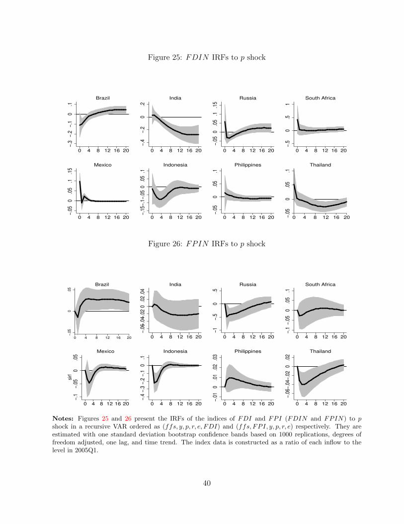
Figure 25: FDIN IRFs to p shock

−.3

−.2

−.1

0.1

0 4 8 12 16 20

Brazil

−.4

−.2

0.2

0 4 8 12 16 20

India

−.05

0.0

5.1

.15

0 4 8 12 16 20

Russia

−.5

0.5

1

0 4 8 12 16 20

South Africa

−.05

0.0

5.1

.15

0 4 8 12 16 20

Mexico

−.15

−.1

−.05

0.0

5.1

0 4 8 12 16 20

Indonesia

−.05

0.0

5.1

0 4 8 12 16 20

Philippines

−.05

0.0

5.1

0 4 8 12 16 20

Thailand

Figure 26: FPIN IRFs to p shock

−.05

0.0

5

0 4 8 12 16 20

Brazil

−.06

−.04

−.02

0.0

2.0

4

0 4 8 12 16 20

India

−1−.

50

.5

0 4 8 12 16 20

Russia−.

1−.

050

.05

.1

0 4 8 12 16 20

South Africa

−.1

−.05

0.0

5si

rf

0 4 8 12 16 20

Mexico

−.4

−.3

−.2

−.1

0.1

0 4 8 12 16 20

Indonesia

−.01

0.0

1.0

2.0

3

0 4 8 12 16 20

Philippines

−.06

−.04

−.02

0.0

2

0 4 8 12 16 20

Thailand

Notes: Figures 25 and 26 present the IRFs of the indices of FDI and FPI (FDIN and FPIN) to pshock in a recursive VAR ordered as (ffs, y, p, r, e, FDI) and (ffs, FPI, y, p, r, e) respectively. They areestimated with one standard deviation bootstrap confidence bands based on 1000 replications, degrees offreedom adjusted, one lag, and time trend. The index data is constructed as a ratio of each inflow to thelevel in 2005Q1.

40

Figure 27: FEVD of FDIN

0.0

5.1

.15

.2

0 4 8 12 16 20

Brazil

0.0

5.1

.15

.20 4 8 12 16 20

India

0.0

5.1

.15

0 4 8 12 16 20

Russia

0.0

2.0

4.0

6.0

8

0 4 8 12 16 20

South Africa

0.0

2.0

4.0

6.0

8

0 4 8 12 16 20

Mexico

0.1

.2.3

.4

0 4 8 12 16 20

Indonesia

0.0

1.0

2.0

3.0

4

0 4 8 12 16 20

Philippines

0.1

.2.3

.4

0 4 8 12 16 20

Thailand

ffs −> FDIN r −> FDIN e −> FDIN p −> FDIN y −> FDIN

Figure 28: FEVD of FPIN

0.0

1.0

2.0

3.0

4

0 4 8 12 16 20

Brazil

0.0

2.0

4.0

6

0 4 8 12 16 20

India

0.0

1.0

2.0

3.0

4.0

5

0 4 8 12 16 20

Russia0

.05

.1

0 4 8 12 16 20

South Africa

0.0

1.0

2.0

3.0

4.0

5

0 4 8 12 16 20

Mexico

0.0

05.0

1.0

15.0

2.0

25

0 4 8 12 16 20

Indonesia

0.0

1.0

2.0

3.0

4

0 4 8 12 16 20

Philippines

0.0

05.0

1.0

15.0

2.0

25

0 4 8 12 16 20

Thailand

ffs −> FPIN y −> FPIN p −> FPIN r −> FPIN e −> FPIN

Notes: Figures 27 and 28 present the FEVD of the indices of FDI and FPI (FDIN and FPIN). Therecursive VAR estimation is ordered as (ffs, y, p, r, e, FDI) and (ffs, FPI, y, p, r, e) for FDIN and FPINrespectively. They are estimated with one standard deviation bootstrap confidence bands based on 1000replications, degrees of freedom adjusted, one lag, and time trend. The index data is constructed as a ratioof each inflow to the level in 2005Q1.

41

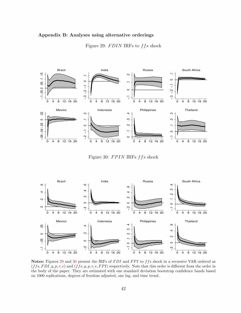
Appendix B: Analyses using alternative orderings

Figure 29: FDIN IRFs to ffs shock−.

1−.0

50

.05

.1.1

5

0 4 8 12 16 20

Brazil

−.3

−.2

−.1

0.1

0 4 8 12 16 20

India

−.1

0.1

.2

0 4 8 12 16 20

Russia

−.3

−.2

−.1

0.1

0 4 8 12 16 20

South Africa

−.06

−.04

−.02

0.0

2

0 4 8 12 16 20

Mexico

−.2

−.1

0.1

.2

0 4 8 12 16 20

Indonesia

0.1

.2.3

.4

0 4 8 12 16 20

Philippines

−.1

0.1

.2.3

0 4 8 12 16 20

Thailand

Figure 30: FPIN IRFs ffs shock

0.2

.4.6

0 4 8 12 16 20

Brazil

−.2

0.2

.4.6

0 4 8 12 16 20

India

−.2

0.2

.4.6

0 4 8 12 16 20

Russia

−.1

0.1

.2.3

.4

0 4 8 12 16 20

South Africa

−.1

−.05

0.0

5

0 4 8 12 16 20

Mexico

−.2

0.2

.4

0 4 8 12 16 20

Indonesia

−.1

0.1

.2.3

.4

0 4 8 12 16 20

Philippines

−.2

0.2

.4.6

0 4 8 12 16 20

Thailand

Notes: Figures 29 and 30 present the IRFs of FDI and FPI to ffs shock in a recursive VAR ordered as(ffs, FDI, y, p, r, e) and (ffs, y, p, r, e, FPI) respectively. Note that this order is different from the order inthe body of the paper. They are estimated with one standard deviation bootstrap confidence bands basedon 1000 replications, degrees of freedom adjusted, one lag, and time trend.

42

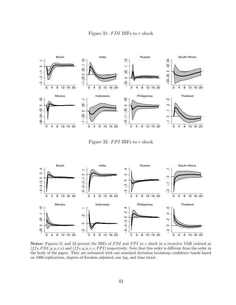
Figure 31: FDI IRFs to r shock

−.3

−.2

−.1

0.1

0 4 8 12 16 20

Brazil

−.1

−.05

0.0

5.1

.15

0 4 8 12 16 20

India

−.05

0.0

5.1

.15

0 4 8 12 16 20

Russia

−.04

−.02

0.0

2.0

4

0 4 8 12 16 20

South Africa

−.06

−.04

−.02

0.0

2

0 4 8 12 16 20

Mexico

−.1

−.05

0.0

5.1

0 4 8 12 16 20

Indonesia

−.15

−.1

−.05

0.0

50 4 8 12 16 20

Philippines

−.1

0.1

.2.3

0 4 8 12 16 20

Thailand

Figure 32: FPI IRFs to r shock

−.6

−.4

−.2

0.2

.4

0 4 8 12 16 20

Brazil

−.4

−.3

−.2

−.1

0.1

0 4 8 12 16 20

India

−.4

−.2

0.2

.4

0 4 8 12 16 20

Russia−.

2−.

10

.1

0 4 8 12 16 20

South Africa

−.05

0.0

5.1

.15

0 4 8 12 16 20

Mexico

−.5

0.5

1

0 4 8 12 16 20

Indonesia

−.6

−.4

−.2

0.2

.4

0 4 8 12 16 20

Philippines

−.2

0.2

.4.6

0 4 8 12 16 20

Thailand

Notes: Figures 31 and 32 present the IRFs of FDI and FPI to r shock in a recursive VAR ordered as(ffs, FDI, y, p, r, e) and (ffs, y, p, r, e, FPI) respectively. Note that this order is different from the order inthe body of the paper. They are estimated with one standard deviation bootstrap confidence bands basedon 1000 replications, degrees of freedom adjusted, one lag, and time trend.

43

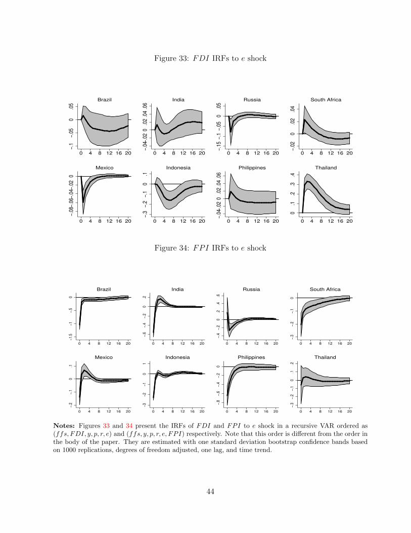
Figure 33: FDI IRFs to e shock

−.1

−.05

0.0

5

0 4 8 12 16 20

Brazil

−.04

−.02

0.0

2.0

4.0

6

0 4 8 12 16 20

India

−.15

−.1

−.05

0.0

5

0 4 8 12 16 20

Russia

−.02

0.0

2.0

4

0 4 8 12 16 20

South Africa

−.08

−.06

−.04

−.02

0

0 4 8 12 16 20

Mexico

−.3

−.2

−.1

0.1

0 4 8 12 16 20

Indonesia

−.04

−.02

0.0

2.0

4.0

60 4 8 12 16 20

Philippines

0.1

.2.3

.4

0 4 8 12 16 20

Thailand

Figure 34: FPI IRFs to e shock

−1.5

−1−.

50

0 4 8 12 16 20

Brazil

−.6

−.4

−.2

0.2

0 4 8 12 16 20

India

−.4

−.2

0.2

.4.6

0 4 8 12 16 20

Russia−.

3−.

2−.

10

0 4 8 12 16 20

South Africa

−.2

−.1

0.1

0 4 8 12 16 20

Mexico

−3−2

−10

1

0 4 8 12 16 20

Indonesia

−.8

−.6

−.4

−.2

0

0 4 8 12 16 20

Philippines

−.3

−.2

−.1

0.1

.2

0 4 8 12 16 20

Thailand

Notes: Figures 33 and 34 present the IRFs of FDI and FPI to e shock in a recursive VAR ordered as(ffs, FDI, y, p, r, e) and (ffs, y, p, r, e, FPI) respectively. Note that this order is different from the order inthe body of the paper. They are estimated with one standard deviation bootstrap confidence bands basedon 1000 replications, degrees of freedom adjusted, one lag, and time trend.

44

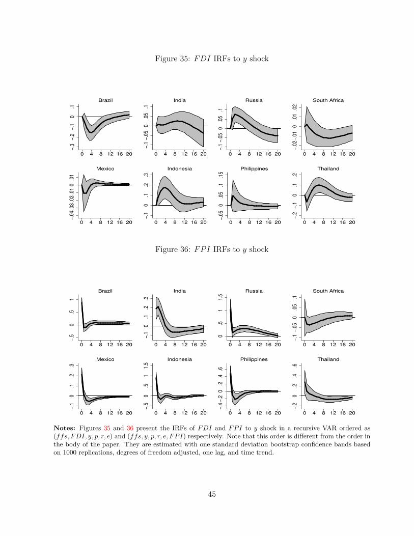
Figure 35: FDI IRFs to y shock

−.3

−.2

−.1

0.1

0 4 8 12 16 20

Brazil

−.1

−.05

0.0

5.1

0 4 8 12 16 20

India

−.1

−.05

0.0

5.1

0 4 8 12 16 20

Russia

−.02

−.01

0.0

1.0

2

0 4 8 12 16 20

South Africa

−.04

−.03

−.02

−.01

0.0

1

0 4 8 12 16 20

Mexico

−.1

0.1

.2.3

0 4 8 12 16 20

Indonesia

−.05

0.0

5.1

.15

0 4 8 12 16 20

Philippines

−.2

−.1

0.1

.2

0 4 8 12 16 20

Thailand

Figure 36: FPI IRFs to y shock

−.5

0.5

1

0 4 8 12 16 20

Brazil

−.1

0.1

.2.3

0 4 8 12 16 20

India

0.5

11.

5

0 4 8 12 16 20

Russia−.

1−.

050

.05

.1

0 4 8 12 16 20

South Africa

−.1

0.1

.2.3

0 4 8 12 16 20

Mexico

−.5

0.5

11.

5

0 4 8 12 16 20

Indonesia

−.4

−.2

0.2

.4.6

0 4 8 12 16 20

Philippines

−.2

0.2

.4.6

0 4 8 12 16 20

Thailand

Notes: Figures 35 and 36 present the IRFs of FDI and FPI to y shock in a recursive VAR ordered as(ffs, FDI, y, p, r, e) and (ffs, y, p, r, e, FPI) respectively. Note that this order is different from the order inthe body of the paper. They are estimated with one standard deviation bootstrap confidence bands basedon 1000 replications, degrees of freedom adjusted, one lag, and time trend.

45

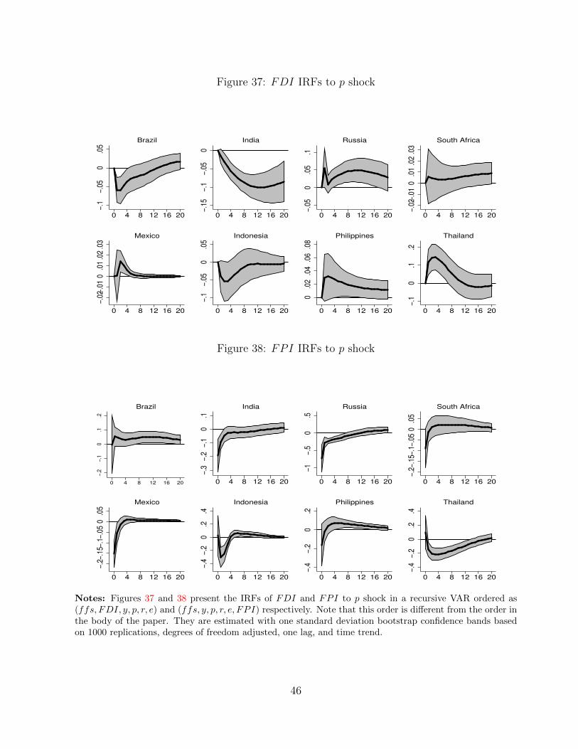
Figure 37: FDI IRFs to p shock

−.1

−.05

0.0

5

0 4 8 12 16 20

Brazil

−.15

−.1

−.05

0

0 4 8 12 16 20

India

−.05

0.0

5.1

0 4 8 12 16 20

Russia

−.02

−.01

0.0

1.0

2.0

3

0 4 8 12 16 20

South Africa

−.02

−.01

0.0

1.0

2.0

3

0 4 8 12 16 20

Mexico

−.1

−.05

0.0

5

0 4 8 12 16 20

Indonesia

0.0

2.0

4.0

6.0

80 4 8 12 16 20

Philippines

−.1

0.1

.2

0 4 8 12 16 20

Thailand

Figure 38: FPI IRFs to p shock

−.2

−.1

0.1

.2

0 4 8 12 16 20

Brazil

−.3

−.2

−.1

0.1

0 4 8 12 16 20

India

−1−.

50

.5

0 4 8 12 16 20

Russia−.

2−.1

5−.1

−.05

0.0

5

0 4 8 12 16 20

South Africa

−.2−

.15−

.1−.

050

.05

0 4 8 12 16 20

Mexico

−.4

−.2

0.2

.4

0 4 8 12 16 20

Indonesia

−.4

−.2

0.2

0 4 8 12 16 20

Philippines

−.4

−.2

0.2

.4

0 4 8 12 16 20

Thailand

Notes: Figures 37 and 38 present the IRFs of FDI and FPI to p shock in a recursive VAR ordered as(ffs, FDI, y, p, r, e) and (ffs, y, p, r, e, FPI) respectively. Note that this order is different from the order inthe body of the paper. They are estimated with one standard deviation bootstrap confidence bands basedon 1000 replications, degrees of freedom adjusted, one lag, and time trend.

46

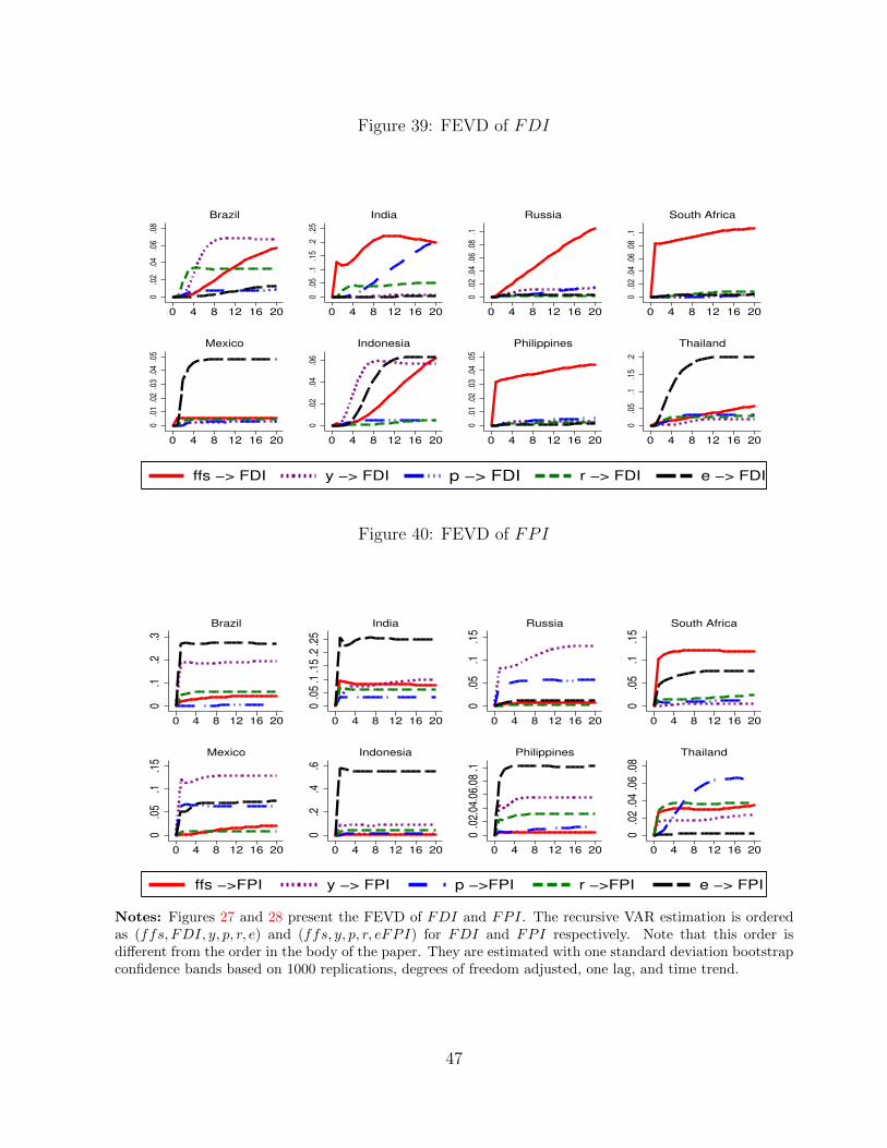
Figure 39: FEVD of FDI

0.0

2.0

4.0

6.0

8

0 4 8 12 16 20

Brazil

0.0

5.1

.15

.2.2

50 4 8 12 16 20

India

0.0

2.0

4.0

6.0

8.1

0 4 8 12 16 20

Russia

0.0

2.0

4.0

6.0

8.1

0 4 8 12 16 20

South Africa

0.0

1.0

2.0

3.0

4.0

5

0 4 8 12 16 20

Mexico

0.0

2.0

4.0

6

0 4 8 12 16 20

Indonesia

0.0

1.0

2.0

3.0

4.0

5

0 4 8 12 16 20

Philippines

0.0

5.1

.15

.2

0 4 8 12 16 20

Thailand

ffs −> FDI y −> FDI p −> FDI r −> FDI e −> FDI

Figure 40: FEVD of FPI

0.1

.2.3

0 4 8 12 16 20

Brazil

0.0

5.1

.15

.2.2

5

0 4 8 12 16 20

India

0.0

5.1

.15

0 4 8 12 16 20

Russia0

.05

.1.1

5

0 4 8 12 16 20

South Africa

0.0

5.1

.15

0 4 8 12 16 20

Mexico

0.2

.4.6

0 4 8 12 16 20

Indonesia

0.0

2.04

.06.

08.1

0 4 8 12 16 20

Philippines

0.0

2.0

4.0

6.0

8

0 4 8 12 16 20

Thailand

ffs −>FPI y −> FPI p −>FPI r −>FPI e −> FPI

Notes: Figures 27 and 28 present the FEVD of FDI and FPI. The recursive VAR estimation is orderedas (ffs, FDI, y, p, r, e) and (ffs, y, p, r, eFPI) for FDI and FPI respectively. Note that this order isdifferent from the order in the body of the paper. They are estimated with one standard deviation bootstrapconfidence bands based on 1000 replications, degrees of freedom adjusted, one lag, and time trend.

47