Dynamic and Instantaneous Pruning of Ensemble Predictors 

  

  

Kaushala Dias    

  

Submitted for the Degree of  Doctor of Philosophy 

 from the University of Surrey 

   

 

 

Centre for Vision, Speech & Signal Processing Faculty of Engineering and Physical Sciences 

University of Surrey Guildford, Surrey GU2 7XH, U.K. 

  

January 2016   

© Kaushala Dias 2016 

AbstractMachine learning research is active in resolving issues that cope with algorithm complexity, efficiency and accuracy in a broad scope of applications, such as face recognition, optical character recognition, data mining, medical informatics and diagnosis, financial time series forecasting, intrusion detection and military applications. In the data representing many of these applications, the issues can be related to high dimensional data with small sample sizes. With large number of features in the data, irrelevant or redundant features can lead to performance degradation due to overfitting, where the predictors may specialise on features which are not relevant for discrimination. To address this, feature selection and ensemble methods have been developed and researched.

In this thesis feature selection has been investigated using feature ranking methods for multiple classifier systems. Recursive Feature Elimination combined with feature ranking is an effective method of removing irrelevant features. An ensemble of Multi-Layer Perceptron (MLP) base classifiers with feature ranking based on the magnitude of MLP weights is proposed along with the extension of this ranking to ensemble pruning.

Also in this thesis ensemble pruning has been investigated for regression with emphasis given to dynamic ensemble pruning as a means of improving accuracy and generalisation. Ordering heuristics attempt to combine accurate yet complementary predictors, and thereby ordering the predictors can lead to enhanced prediction accuracy and generalisation. A dynamic method is proposed that enhances the performance by modifying the order of aggregation through distributing the ensemble selection over the entire dataset. Two more dynamic methods have been proposed that implement ensemble pruning by diverse predictor selection in the learning process. The first of these two methods simultaneously prunes and trains in the same learning process, while the second method is a hybrid method that applies different learning approaches selectively. Experimental results demonstrate improved performance for dynamic ensemble pruning on benchmark datasets and an application in signal calibration.

Key Words: Ensemble Methods, Dynamic Ensemble Pruning

   

AcknowledgmentI wish to extend my sincere appreciation and thanks to my supervisor Dr. Terry Windeatt for the technical advice and guidance in the subject matter as well as in general about life in the world of machine learning research. I also would like to thank my co-supervisor Professor Josef Kittler for his advice and guidance in machine learning. My thanks go to my colleagues at EW Simulation Technology and CVSSP for the discussions in their respective fields of work and for the support and assistance afforded to my research.

This research degree has been undertaken in collaboration with EW Simulation Technology Limited (EWST). Therefore I wish to thank EWST and in particular John Parsons of EWST for offering me the opportunity and the platform to research methods to reduce calibration times of their hand-held radar simulator product line. I would also like to thank EWST for the use of their facilities and equipment for the experiments carried out on the calibration application.

Finally I would like to thank my family, especially my wife Shakya and my two lovely children Vishudhi and Januthi for their patience, encouragement and support and my parents Dr. Malini Dias and Jeevananda Dias for their support and encouragement.

v  

ContentsList of Tables viii

List of Figures ix

1 An Introduction to Feature Selection, Ensemble Predictors and Dynamic

Ensemble Pruning 1

1.1 Motivation ........................................................................................................ 1

1.1.1 Curse of Dimensionality and Overfitting ............................................. 1

1.1.2 Ensemble Methods and Pruning ........................................................... 3

1.1.3 Signal Calibration using Neural Networks ........................................... 4

1.2 Objectives ......................................................................................................... 5

1.3 Contributions .................................................................................................... 6

1.4 List of Publications ........................................................................................... 8

1.5 Structure of the Thesis ...................................................................................... 9

2 Literature Review and Background Study 10

2.1 Introduction .................................................................................................... 10

2.2 Feature Selection ............................................................................................ 14

2.3 Ensembles ....................................................................................................... 16

2.4 Ensemble Pruning ........................................................................................... 21

2.5 Conclusion ...................................................................................................... 30

3 Feature Ranking and Ensemble Approaches for Classification 32

3.1 Introduction .................................................................................................... 32

3.2 Multiple Classifier System ............................................................................. 35

3.3 Feature Ranking ............................................................................................. 38

3.3.1 Ranking by Classifier Weights (rfenn, rfesvc) ................................... 40

3.3.2 Ranking by Noisy Bootstrap (rfenb) .................................................. 41

3.3.3 Ranking by Boosting (boost) .............................................................. 41

3.3.4 Ranking by Statistical Criteria (1 dim, SFFS) .................................... 42

3.4 Datasets .......................................................................................................... 43

3.5 Experimental Evidence ................................................................................... 45

vi  

3.5.1 Performance variation with the number of Features (ranked) and Training Sample Size for the Base and Ensemble classifier on the 2-class dataset ............................................................................... 47

3.5.2 Performance by Ensemble classifier and SVC on the 2-class dataset for features ranking methods .................................................. 48

3.5.3 Features ranked between Ensemble classifier and SVC on the

face dataset ......................................................................................... 50

3.6 Conclusion ...................................................................................................... 52

4 Dynamic Ensemble Selection and Instantaneous Pruning for Regression 54

4.1 Introduction .................................................................................................... 54

4.2 Ensemble Pruning ........................................................................................... 55

4.2.1 Ordered Aggregation pruning ............................................................. 56

4.2.2 Recursive Feature Elimination Pruning .............................................. 58

4.2.3 Pruning Optimisation Using Genetic Algorithms .............................. 59

4.2.4 Reduced Error Pruning ....................................................................... 60

4.2.5 Dynamic Ensemble Pruning ............................................................... 61

4.3 Method ............................................................................................................ 62

4.4 Experimental Evidence ................................................................................... 65

4.4.1 Performance variation between Static Pruning methods and the

proposed Dynamic Pruning method ................................................... 68

4.4.2 Performance variation of pruning with different distance

measures ............................................................................................. 69

4.5 Conclusion ...................................................................................................... 70

5 Hybrid Dynamic Learning Systems for Regression 72

5.1 Introduction .................................................................................................... 72

5.2 Pruning and Hybrid Learning ......................................................................... 74

5.2.1 Ensemble Learning with Dynamic Ordering Pruning ........................ 75

5.2.2 Hybrid Ensemble Learning with Dynamic Ordered Pruning ............. 76

5.3 Methods .......................................................................................................... 77

5.3.1 ELDOP ............................................................................................... 77

5.3.2 HELDOS ............................................................................................ 79

5.4 Experimental Evidence ................................................................................... 81

5.5 Conclusion ...................................................................................................... 84

vii  

6 Signal Calibration using Ensemble Systems 86

6.1 Introduction .................................................................................................... 86

6.2 Signal Calibration ........................................................................................... 89

6.2.1 Learning the Calibration Function ...................................................... 90

6.2.2 Training Methods for the Learning Model ......................................... 93

6.3 Results ............................................................................................................ 94

6.4 Conclusion ...................................................................................................... 96

7 Conclusion and Future Work 97

7.1 Conclusion ...................................................................................................... 97

7.2 Limitations .................................................................................................... 100

7.3 Future Work ................................................................................................. 101

Bibliography 103

viii  

ListofTables3.1 Facial Action Units (au) – six upper face aus around the eyes ................................ 34

3.2 Benchmark datasets used for experiments showing the number of patterns,

continuous and discrete features and estimated Bays error rate .............................. 43

3.3 Mean best error rates (%)/number of features for seven two-class problems

(20/80) with five feature-ranking schemes (Mean 10/90, 5/95 also shown) ........... 49

3.4 Mean best error rates (%)/number of features for au1 classification 90/10 with

five feature-ranking schemes ................................................................................... 50

3.5 ECOC super-classes of action units and number of patterns ................................... 51

3.6 Mean best error rates (%) and area under ROC showing #nodes /#features for au

classification 90/10 with optimized PCA features and MLP ensemble .................. 51

4.1 Benchmark datasets used for experiments showing the number of patterns and

features ..................................................................................................................... 65

4.2 Static Ensemble Pruning Methods: Averaged MSE with Standard Deviation for

the 100 iterations ...................................................................................................... 68

4.3 DESIP with Static Methods Adopted: Averaged MSE with Standard Deviation

for the 100 iterations ................................................................................................ 68

4.4 Comparison of the minimum average ensemble size: Static Method / DESIP

with Static Method Adopted .................................................................................... 69

4.5 Averaged MSE of DESIP – Using Euclidean distance ............................................ 69

4.6 Averaged MSE of DESIP – Using Mahalanobis distance ....................................... 70

5.1 Benchmark datasets used for experiments showing the number of patterns and

features ..................................................................................................................... 81

5.2 Averaged MSE of the test set with Standard Deviation for 10 iterations for NCL,

OA, DESIP, ELDOP and HELDOS ........................................................................ 81

6.1 Average MSE with Standard Deviation for 10 iterations, OA, RFE and

DESIP/RE ................................................................................................................ 95

6.2 Average MSE with Standard Deviation for 10 iterations, NCL, OA, DESIP,

ELDOP and HELDOS ............................................................................................. 95

ix  

ListofFigures1.1 Curse of Dimensionality ............................................................................................ 2

1.2 Block diagram of the RF source device’s function .................................................... 5

3.1 Mean test error rates, Bias, Variance for RFE perceptron ensemble with Cancer

Dataset 20/80, 10/90, 5/95 train/test split ................................................................ 47

3.2 Mean test error rates, Bias, Variance for RFE MLP ensemble over seven 2-class

Datasets 20/80, 10/90, 5/95 train/test split ............................................................... 48

3.3 Mean test error rates, True Positive and area under ROC for RFE MLP ensemble

for au1 classification 90/10, 50/50 train/test split .................................................... 50

4.1 Comparison of Ordered Aggregation Vs Random Ordered ensemble prediction

error .......................................................................................................................... 57

4.2 Pseudo-code implementing the archive matrix with ordered ensemble per

training data ............................................................................................................. 64

4.3 Pseudo-code implementing the identification of the nearest training pattern to

the test pattern .......................................................................................................... 64

4.4 Comparison of the MSE plots of the training set and the test set for OA, RFE

and DESIP using RE ........................................................................................... 66/67

5.1 Pseudo-code implementing the training process with ordered ensemble pruning

per training pattern for the ELDOP method ............................................................ 77

5.2 Pseudo-code implementing the ensemble output evaluation for test pattern ........... 79

5.3 Pseudo-code implementing the training process with ordered ensemble pruning

per training pattern for the HELDOS method ......................................................... 80

5.4 Comparison of the MSE plots of the training set and the test set for NCL,

ELDOP and HELDOS ........................................................................................ 82/83

6.1 Calibration with signal correction using model of nonlinear system ...................... 89

6.2 Calibration with correct signal provided by a model that has learnt the corrective

action ........................................................................................................................ 90

6.3 Block diagram of RTS with Learned Model providing Correct Control Signals .... 91

x  

6.4 Training and Interrogation of Neural Networks for the Learned Model ................. 92

6.5 Non-linear characteristics and the calibrated characteristics of the Radio

Frequency Source Device ........................................................................................ 93

6.6 Calibration application MSE performance of OA, RFE and DESIP using RE ....... 95

6.7 Calibration application MSE performance of NCL, OA, DESIP, ELDOP and

HELDOS .................................................................................................................. 95

1  

Chapter1

An Introduction to Feature Selection, Ensemble Predictors and Dynamic Ensemble Pruning

In this chapter a general introduction to feature selection, ensemble methods and

dynamic pruning is presented, along with the motivation for the current research,

the approaches, objectives, contributions and the structure of this thesis.

1.1 Motivation

Machine learning is used in applications such as information technology, clinical decision

support systems, image and signal processing where they make decisions based on input

stimuli. These stimuli are in general features that represent the observable domain of the

application. The observable domain in some applications can have large numbers of features,

running into hundreds and thousands of features, with small sample sizes leading to increased

complexity and degradation in efficiency and accuracy of the predictors. The curse of

dimensionality and over-fitting are related problems with high dimensional small sized

training samples and the resulting predictor works well with the training data but very poorly

with test data.

1.1.1 Curse of Dimensionality and Overfitting

The curse of dimensionality is associated with multivariate data analysis as the number of

dimensions increase. In high dimensional data the complexity and the difficulty in training a

predictor increases with the number of features. However at a given number of features a

2  

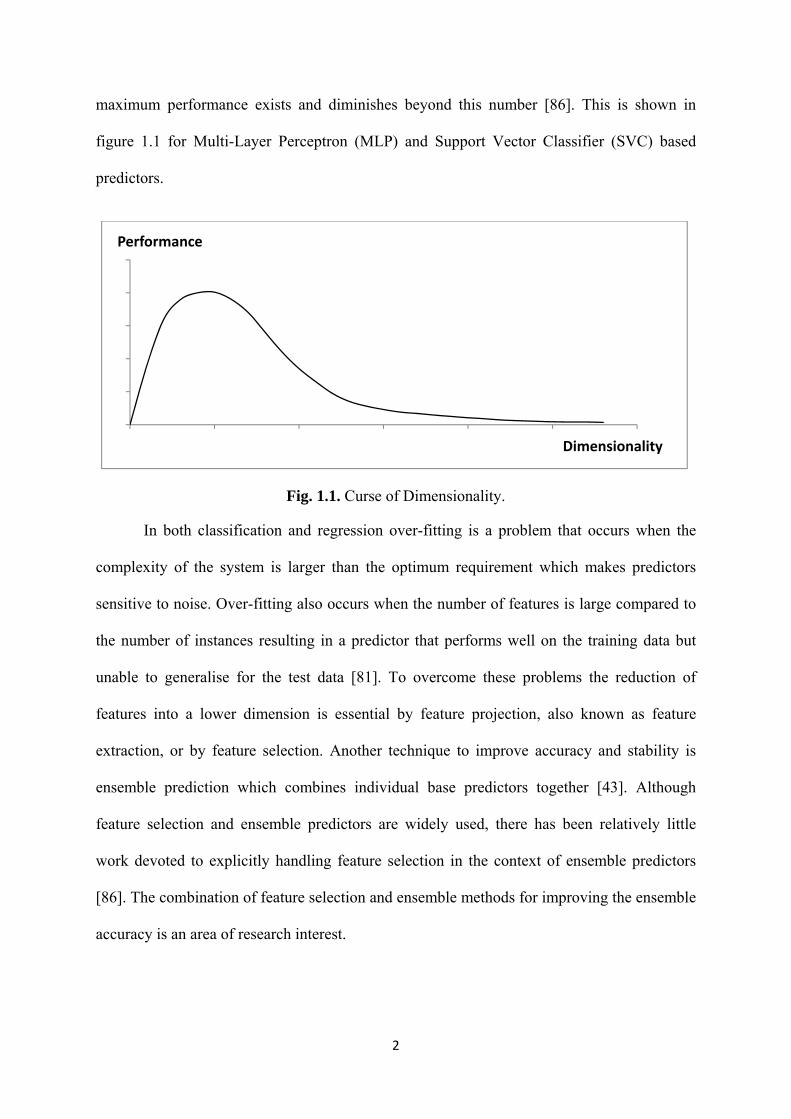
maximum performance exists and diminishes beyond this number [86]. This is shown in

figure 1.1 for Multi-Layer Perceptron (MLP) and Support Vector Classifier (SVC) based

predictors.

Fig. 1.1. Curse of Dimensionality.

In both classification and regression over-fitting is a problem that occurs when the

complexity of the system is larger than the optimum requirement which makes predictors

sensitive to noise. Over-fitting also occurs when the number of features is large compared to

the number of instances resulting in a predictor that performs well on the training data but

unable to generalise for the test data [81]. To overcome these problems the reduction of

features into a lower dimension is essential by feature projection, also known as feature

extraction, or by feature selection. Another technique to improve accuracy and stability is

ensemble prediction which combines individual base predictors together [43]. Although

feature selection and ensemble predictors are widely used, there has been relatively little

work devoted to explicitly handling feature selection in the context of ensemble predictors

[86]. The combination of feature selection and ensemble methods for improving the ensemble

accuracy is an area of research interest.

0

5

10

15

20

25

0 5 10 15 20 25 30

Performance

Dimensionality

3  

1.1.2 Ensemble Methods and Pruning

In machine learning, an ensemble is defined as a group of learning models of which the

outputs are combined to produce a unified output. The ensemble predictor outputs can be

combined simply by taking a vote among individual models which are trained independently

on the given problem, or in a more complex way such as combining models to be trained

consecutively to compensate for the weaknesses of each other [50]. Ensembles are used in

regression as well as classification.

Many different methods of generating and combining predictors have emerged from

the research conducted over the past decade. With this, ensembles have become preferable

over single predictors due to their advantages in terms of accuracy, complexity and

flexibility. However there are still issues with ensembles that need attention, such as the

accuracy-diversity dilemma [77]. Here, on the one hand, it would be beneficial to have

predictors with high accuracy, while on the other hand it is desired that they are uncorrelated

so as to benefit from their differences. However, with increased accuracy predictors tend to

be similar which lack diversity.

Another issue is ensemble selection, also known as pruning, where member predictors

of the ensemble are selected in order to improve accuracy and generalisation [69]. In some

cases pruning is attributed to algorithm and memory efficiency. Many pruning methods and

theoretical approaches have emerged in the research to date that suggests pruning achieves

better performance than when the ensemble is taken as a whole. There exists a sub-ensemble

within the full ensemble with lower error than the ensemble taken as a whole [109]. A

parallel can be drawn between feature selection and ensemble pruning, where ensemble

members are considered as features and the aim is to reduce the ensemble size by selecting

4  

the members that aren’t redundant or irrelevant and effectively improve the performance,

where a maximum is reached at a reduced set of features or smaller ensemble size.

Dynamic ensemble pruning methods, in contrast to static pruning methods, make a

selection of predictors for each test pattern. Therefore, dynamic methods potentially deliver a

different sub-ensemble for every test pattern with improved performance, compared to static

methods that can only provide a fixed ensemble for all test patterns [111]. The majority of the

dynamic methods start by retrieving the k nearest neighbours of a given test instance from the

training set to form the local region for pruning the ensemble. Then based on properties such

as accuracy and diversity, selection algorithms decide the appropriate subsets of predictors

for the pruned ensemble. Clustering based and ordering based methods have also been used

for dynamic ensemble selection. Although many researchers have worked on ensemble

pruning for classification, there has been relatively little on regression.

1.1.3 Signal Calibration using Neural Networks

A calibration application is presented in this thesis to demonstrate the use of neural networks

as a means of learning the corrective action to linearize a nonlinear device. Usually, in the

absence of feedback from the output of a nonlinear device, a model of this device is used to

seek behavioural parameters to calculate the corrections that are applied to linearize the

device. However, by learning the corrective actions, it’s possible to directly apply corrections

to linearize the output, bypassing the need to calculate the corrections from a model.

Therefore neural networks are used for learning this corrective action.

The application described in this thesis consists of a Radio Frequency (RF) source

device, with amplitude control, that functions within a handheld radar threat simulator. A

block diagram of this device’s function is shown in figure 1.3., where the amplitude of the

5  

output RF signal, which is controlled by the attenuator function, is nonlinear – i.e. the user

demanded attenuation and the attenuation of the output RF signal has a nonlinear

relationship. Using the generalising ability of neural networks, the application aims to create

a neural network model with training samples containing features of the nonlinear device and

to use this model to linearize the attenuation of the output RF signal. Here the investigated

static and dynamic ensemble pruning methods are applied to enhance the accuracy and the

generalisation performance of the neural network model.

Fig. 1.2. Block diagram of the RF source device’s function.

This thesis aims to describe research that enhances prediction accuracy and efficiency

using dynamic pruning of ensemble methods as stated in the following objectives.

1.2 Objectives

The main aim of the research is to improve the accuracy of ensemble predictors by means of

dynamic ensemble pruning methods. A secondary aim is to improve the calibration of a

nonlinear device for an industrial application using the benefits of dynamic ensemble pruning

approaches in regression. The main objectives of this research are as follows:

Attenuator Function 

RF In

Attenuation Demand 

Frequency 

Output  Attenuation

 

RF Source 

RF Out

6  

1. Investigate the use of Multi-Layer Perceptron for feature ranking for the purpose of

feature selection. Propose selection methods based on feature ranking for ensemble

pruning.

2. Study the static and dynamic ensemble pruning approaches and compare state of the art

ordered pruning methods. Propose new dynamic ensemble pruning methods for

regression.

3. Investigate the diversity encouraging mechanisms of regression ensembles and propose

hybrid learning mechanisms that encourage diversity among predictors.

4. Investigate the use of pruned ensembles in an industrial calibration application consisting

of a nonlinear Radio Frequency device. In the investigation, the goal is to improve the

predictor accuracy by applying the dynamic ensemble pruning methods.

1.3 Contributions

Starting with feature selection for ensembles, a pruning method has been proposed and

compared with other static and dynamic ensemble pruning methods that encourage diversity

in ensemble predictors. Novel dynamic pruning methods have been proposed and applied to

an application for improving predictor accuracy in nonlinear device calibration. The detailed

contributions in each chapter in this thesis are described below:

An ensemble of Multi-Layer Perceptron (MLP) base classifiers with feature-ranking

based on Recursive Feature Elimination (RFE) using the magnitude of MLP weights is

proposed. Experimental results of this method are compared with Principal Component

Analysis and other popular feature-ranking methods using high dimensional data. By posing

as a multi-class problem using Error-Correcting-Output-Coding (ECOC), error rates are

compared to two-class problems with optimised number of features and base classifier.

7  

Based on the method of Recursive Feature Elimination (RFE) a novel ensemble predictor

ranking method for ensemble pruning is proposed. Here the weights of a neural network have

been utilised for ranking the inputs of a trained combiner, which are the outputs of the

ensemble predictors. This method has been used in regression as a static as well as a dynamic

pruning method. A novel dynamic ensemble pruning approach is proposed for improving the

prediction accuracy and generalisation of the ensemble, that change the order in which

ensemble predictors are combined. The proposed method modifies the order of aggregation

through distributing the ensemble selection over the entire training set, which is then

dynamically used based on closeness of a test pattern to the training patterns. This dynamic

method is compared, using the Reduced Error Pruning Method without Back Fitting, with

other static methods as well as incorporating them in this dynamic approach.

Methods of encouraging diversity in the learning process of regression ensemble

predictors have been investigated. With this, two dynamic methods have been proposed, one

involving pruning and the other a hybrid method. In these methods diversity is introduced

while simultaneously training as part of the same learning process but selectively trained,

resulting in a diverse selection of predictors that have strengths in different parts of the

training set.

Dynamic pruning methods for the calibration of a nonlinear Radio Frequency source

device have been compared with other state-of-the art techniques. The main objective is to

improve prediction accuracy of ensemble methods when applied to the calibration

application. The learning methods proposed address the non-existent use of learning systems

to provide corrective measures for direct linearization of nonlinear devices.

8  

1.4 List of Publications

The research presented in this thesis has been submitted and presented at different

international venues related to pattern recognition, neural networks, machine learning,

computational intelligence and intelligent signal processing. These publications are as

follows, based on their contribution within the structure of this thesis:

1. T. Windeatt , K. Dias, Feature Ranking Ensembles for Facial Action Unit

Classification, Artificial Neural Networks in Pattern Recognition, ANNPR, Third IAPR

Workshop, Springer, LNCS 5064, pp 267 – 279, 2008.

2. T. Windeatt, K. Dias, Ensemble Approaches to Facial Action Unit Classification,

CIARP, 13th Iberoamerican Congress on Pattern Recognition, Springer, LNCS 5197, pp 551

– 559, 2008.

3. K. Dias, T. Windeatt, Dynamic Ensemble Selection and Instantaneous Pruning for

Regression, European Symposium on Artificial Neural Networks, Computational Intelligence

and Machine Learning, ESANN, pp 643 – 648, 2014.

4. K. Dias, T. Windeatt, Dynamic Ensemble Selection and Instantaneous Pruning for

Regression used in Signal Calibration. International Conference on Artificial Neural

Networks, ICANN, Springer, LNCS 8681, pp 475 – 482, 2014.

5. K. Dias, T. Windeatt, Ensemble Learning with Dynamic Ordered Pruning for

Regression, European Symposium on Artificial Neural Networks, Computational Intelligence

and Machine Learning, ESANN, pp 125 – 130, 2015.

6. K. Dias, T. Windeatt, Hybrid Dynamic Learning Systems for Regression, 13th

International Work-Conference on Artificial Neural Networks, Advances in Computational

Intelligence, LNCS 9095, pp 464 – 476, 2015.

9  

7. K. Dias, Direct Signal Calibration using Learning Systems, Intelligent Signal

Processing - Conference, IET, London, 2nd December 2015.

8. K. Dias, EW Simulation Technology, A System of Providing Calibration Information

to a Radio Frequency Attenuator Means, UK Patent Application Number: GB1313351,

International Patent Number: WO2015011496 A1, 2015.

1.5 Structure of the Thesis

The overall structure of this thesis is as follows: literature review and background study of

feature selection, ensembles and ensemble pruning is described in chapter 2. Chapter 3

presents feature ranking and ensemble approaches for classification as well as proposing RFE

as a means of feature selection. Chapter 4 proposes RFE as a means of ensemble ranking for

ensemble pruning, along with dynamic ensemble selection and instantaneous pruning for

regression. Chapter 5 proposes diversity encouraging mechanisms for ensemble learning and

pruning with two methods proposed for regression. In Chapter 6 an industrial application has

been described where a neural network ensemble has been used as a learning system for

direct signal calibration. Finally, conclusions and future work are summarised in Chapter 7.

 

10  

Chapter2

Literature Review and Background Study

Ensemble selection and pruning in classification and in regression have been

extensively studied by researchers for many years in order to improve prediction

performance. In addition, dynamic pruning and selection benefits performance

by evaluating the best subset of the ensemble available to predict accurately.

This chapter presents a general literature survey and background study of

ensemble pruning and selection encompassing both static and dynamic domains.

Chapters 3 to 5 contain their own literature reviews tailored to each chapter. The

remainder of this chapter is organised as follows: Feature Selection in section

2.2, Ensembles in 2.3 and Ensemble Pruning in section 2.4.

2.1 Introduction

An ensemble of predictors, whether classifiers for predicting classes or regressors for

continuous real valued predictions, is well known for improving the prediction accuracy [1].

Here the predictions of a group of base predictors that learn a target function are combined

together to form the overall prediction. The underlying principle of ensemble learning is that

in real world situations a trained model will not be a perfect device that predicts accurately

and will make errors. With this the aim of ensemble learning is to manage their strengths and

weaknesses to increase the prediction accuracy [2]. An ensemble has the ability to increase

the prediction accuracy by combining the outputs of multiple experts, improve efficiency by

decomposing a complex problem into a multiple of sub-problems and improve reliability by

reducing uncertainty. With this an ensemble has the improved ability to generalise for new

11  

unseen patterns. Of the many ensemble methods available, Bagging [3] and Boosting [4] are

well known in machine learning.

Feature reduction is an essential part in the generation of accurate predictors. With

high dimensional data, some features can be irrelevant or redundant, and cause degradation in

predictor performance as well as increased complexity in obtaining useful samples when

training samples are scarce relative to the number of features. There are two approaches to

feature reduction: feature extraction and feature selection. In feature extraction, original

features are transformed into lower dimensional features by projection. No prior knowledge

of the data is required for this process, however the new features are difficult to understand

due to the altered semantics of the original features. Commonly used methods of this type are

Principle Component Analysis (PCA) [5] and Linear Discriminant Analysis (LDA) [6].

PCA, being an unsupervised method, does not take class labels into account when extracting

features. It transforms the original features in the direction of maximum information, and

thereby reducing features. LDA on the other hand is supervised, and reduces dimensionality

by sampling within-class and between-class separation and projecting the original features in

the direction that maximises between-class separation and minimises the within-class

separation. In feature selection, feature reduction is achieved by removing irrelevant and

redundant features leaving an optimal set of features from the original set. This feature

reduction is performed as a pre-processing step and the maximum performance is achieved

with this optimal minimum number of features.

The method of combining predictions has been of interest to several fields over many

years and has yielded many methods, such as averaging, voting, linear and nonlinear

combining, stacking etc. To benefit from the coming together of members of the ensemble,

each member should be either unique or provide diversity among the members. That is, two

12  

similar predictors that do not have new information between them about their decision

boundaries would not be advantageous to the ensemble. Therefore being diverse essentially

improves the ensemble performance. There are two categories of ensemble learning

algorithms that encourage diversity. They are the categories of implicit and explicit diversity

encouraging methods. The vast majority of ensemble methods are implicit methods, where

they provide different random sub-sets of the training data, and thereby randomly sample the

dataspace to implicitly cause diversity in the predictors. Examples of methods that implicitly

encourage diversity are Bootstrapping of random training patterns, Random Subspace

Method (RMS) [7] for selecting different features in the training pattern, Error Correcting

Output Coding (ECOC) [8] providing random classes and Multi-layer Perceptron that

initiates with random weights. In the explicit methods, diversity is encouraged by

constructing each ensemble member with some measurement that ensures it is considerably

different from the other members. Examples in this category are Boosting which trains each

predictor with a different distribution of the training set and Negative Correlation Learning

(NCL) that includes a penalty term when learning each predictor. With diversity encouraged

in this manner, there however exists a trade-off between the accuracy and diversity of the

ensemble that should be taken account of. This is known to be the accuracy/diversity

dilemma [9].

In order to overcome an important short-coming of ensemble methods when large

ensembles are produced that contains predictors that aren’t useful in the combined prediction,

an intermediate phase that removes these predictors is introduced. Also known as ensemble

pruning or ensemble selection, the technique methodically removes predictors to improve

efficiency and generalisation performance. Pruned sub-ensembles can in effect outperform

the original ensembles from which they are selected [10] [11]. The search for the optimal

sub-ensemble from a pool of predictors is a difficult problem, one that requires searching in

13  

the space of 2M – 1 non-empty sub-ensembles that can be extracted from an ensemble of size

M [12]. Even after searching for the optimal sub-ensemble, the search will be based in terms

of an objective function of the training data, where by it cannot be guaranteed for out-of-

sample performance to be optimal. Therefore to solve this problem, approximate algorithms

that select near-optimal sub-ensembles with high probability of accuracy are proposed [13].

Here the predictors considered are classifiers as well as regressors, however more attention

has been given to classifiers than regressors in the literature.

In contrast to Static pruning, where a fixed subset of the ensemble is selected for all

test instances, Dynamic ensemble pruning, also known as instance based pruning, selects a

different subset of predictors from the original ensemble for each test instance. The rationale

for using dynamic ensemble pruning approaches is that different predictors have varied levels

and areas of expertise in the instance space. Another dynamic approach is to select only one

predictor from a pool of predictors, that is most likely to be correct for a test instance [14]. In

the ensemble pruning approaches where the pruned ensemble is still an ensemble of

predictors, it is assumed that the member predictors are independent in their errors and are

reliable in their individual predictions. However in the case where a single predictor is

selected, this assumption is not taken into consideration [15]. In industrial applications,

dynamic ensemble approaches for adaptive model development are favoured due to their

ability to model the changing conditions of industrial processes [16]. In this case the dynamic

methods, such as Sliding Window (SW) and Just-in-Time Learning (JITL) have been

proposed. With SW, a new model is trained by a moving window that incorporates new

samples of the changing conditions as they become available. JITL creates a temporary local

model using samples that are similar to a test sample, and after the prediction for the test

sample the local model is discarded.

14  

2.2 Feature Selection

There has been extensive research on feature selection carried out in the fields of machine

learning, statistics and data mining. Initial focus was on relevance analysis in which

irrelevant features were removed from the original feature set, such as ID3 [17], FOCUS

[18], RELIEFE [19] and CFS [20]. It is proposed in the ID3 decision tree algorithm to use

information gain to select relevant features. In FOCUS all subsets of features are searched

exhaustively for the minimum subset of features which is sufficient for determining the class

label to construct a small decision tree. In RELIEFE relevant features are selected statistically

by evaluating a random subset of samples and calculating the average difference in distance

for the nearest samples of the same class (near-hit) and different class (near-miss). However

if most features are relevant, RELIEFE may possibly select redundant features too [21]. In

order to improve the accuracy of predictors the wrapper methods for feature selection were

introduced [22]. The wrapper method’s selection of features is based on the learning

algorithm used for training the predictors. It evaluates feature subsets using classifier

accuracy. A probabilistic approach using Las Vegas Algorithm (LVF) is proposed as filter

method for feature selection [23]. Filter methods function as a pre-processing step which is

independent of the learning algorithm. This method searches for the optimal features using a

scoring function. Mutual Information, Information Gain, Statistic Test and Markov Blanket

are commonly used scoring functions. Wrapper methods usually outperform filter methods

as they take predictive performance into account. However it’s computational time is

significant and might easily over-fit high dimensional feature spaces. In [24] a hybrid method

of searching feature subsets is shown using a combination of LVF for reducing the number of

features and Automatic Branch and Bound (ABB) for completing the search for optimal

subsets on this reduced feature set. Feature selection for clustering is presented in [25].

Genetic algorithm for feature selection using randomised heuristic search is presented in [26].

15  

Correlation-based Feature Selection (CFS) proposed in [20] by Hall, is a well-known feature

selection technique that removes irrelevant features. In addition to relevance analysis,

redundancy analysis has been extensively investigated. Yu and Liu proposed Fast

Correlation-based Filter (FCBF) algorithm in [27] [28] to remove irrelevant and redundant

features by using Symmetrical Uncertainty (SU). Malarvili et al. [29] proposed relevance and

redundancy analysis technique based on discriminant analysis using area under ROC curve

and predominant features based on discriminant power for redundancy analysis in Neonatal

Seizure Detection application. Deisy et al. [30] proposed Decision Independent Correlation

(DIC) and Decision Dependent Correlation (DDC) to remove irrelevant and redundant

features, respectively. Biesiada and Duch [31] use SU to remove irrelevant features and used

Pearson X2 test to eliminate redundant features for biomedical data analysis. In [32]

Kolmogorov-Smirnov algorithm was proposed to reduce redundant and irrelevant features.

From the empirical bias and variance analysis performed on feature selection by Munson and

Caruana [33] suggests that the improvement of classifier performance is due to the decrease

in variance, and not due to the decrease in number of noisy features or separating irrelevant

features from the relevant. There exists a trade-off between reduction in variance and increase

in bias. A similar concept proposed by Yu and Liu [28] suggests that the optimal feature

subset should not only contain strongly relevant features but also weakly relevant features

which have no redundancy or irrelevant features.

Other methods of feature selection used, apart from the filter and wrapper methods,

are embedded and hybrid methods. In embedded methods, optimal subset of features is

selected during learning. Decision trees and Support Vector Machine-Recursive Feature

Elimination (SVM-RFE) [34] are well known embedded methods. In hybrid feature selection

the combined benefits of both filter and wrapper methods are exploited [35].

16  

Searching for feature subsets can be sequential or random. A complete exhaustive

search of possible subsets from N original features is 2N [36] and a well-known complete

search method is branch and bound [37]. Since it may be impractical to exhaustively search

large number of features, heuristic search is more common. In sequential search features are

either added or eliminated sequentially. This method is fast and the complexity is less than or

equal to O(N2). However it is possible to converge to local minima using this method.

Examples of sequential search methods are Sequential Forward Selection (SFS), Sequential

Backward Selection (SBS), Plus-l-take-away-r [38], and Sequential Floating Search (SFFS

and SBFS) [39]. Random search methods randomly add or remove features and are able to

solve problems relating to local minima. Examples of random search methods are Genetic

Algorithm [26] and simulated annealing [40].

2.3 Ensembles

Ensemble predictors have been primarily used for improving generalisation as well as

accuracy of predictions. Hanson and Salamon [41] improved generalisation by using neural

network multiple classifiers, due to their unstable nature. Dietterich et al. [8] proposed, as a

necessary condition, that base classifiers in ensemble classifiers should be accurate and

diverse for the ensemble to be accurate. Schapire [42] presented the Boosting algorithm to

improve weak classifiers, by randomly sampling the data without replacement to create

classifiers iteratively and then combining these classifiers by majority vote. The classifiers

thus created use a different distribution of samples on every iteration [43] [44]. The resulting

ensemble of classifiers has an accurate prediction rule that consists of many inaccurate rules

of thumb. AdaBoost is proposed in [4] as an improved version of the Boosting algorithm.

AdaBoost also manipulates the training samples to create classifiers iteratively and combines

with a weighted majority vote. Here the classification error of each classifier on the training

17  

samples is used to weight the samples, where the weight attached to a sample is proportionate

to the classification error. Based on these weights a sample with a higher weight will be used

for training the next classifier. Therefore training samples that are misclassified most by the

previous classifiers gets used in the training of the next classifier. The outputs of the final

ensemble of classifiers are combined with weighted majority vote [42]. AdaBoost is less

susceptible to low noise conditions, however over-fitting can occur in high noisy conditions

due to increased weight on misclassified samples [8].

Breiman [3] introduced bagging to improve accuracy in ensemble classifiers, by

creating predictors trained with bootstrapped samples from the training data and combining

with a majority vote. Each bootstrap is a random selection of samples with replacement.

Bagging shows tolerance to noisy data with small sample size. However as sample size gets

larger the performance may degrade due to the reduction in diversity among the bootstrap

samples owing to their similarity. Random Subspace Method (RSM) [7] creates ensemble

classifiers by randomly selecting feature subsets for decision tree base classifiers. Input

Decimation (ID) [45] also manipulates feature space to select feature subsets for creating

ensemble classifiers. Breiman [46] also proposed Random Forests which combines Bagging

with Random Subspace Methods for base classifiers consisting of decision trees. In this

method, multiple trees are created with bootstrap samples and at each branch of a decision

tree, features are randomly selected from the original set of features [47] [2]. Rotation Forests

[48] also creates ensemble decision trees by randomly selecting features subsets from the

original data and using Principal Component Analysis transforms each features subset for

final combined output.

In a comparison of theoretical frameworks for combining classifiers in [49], Kittler et

al. suggests that the sum rule performs better than other combination rules, such as minimum,

18  

maximum, median, product rule and majority vote. A review of the ensemble methods has

been performed by Deitterich in [50] using Bayesian average, error-correcting output coding,

Bagging and Boosting, and explains why an ensemble of classifiers usually outperforms a

single classifier. In the well-known reference publication of methods and algorithms of

ensemble classifiers [43] and [51], Kuncheva provided the formulae for the probability of

error for six classifier fusion methods: average, minimum, maximum, median, majority vote

and oracle. Polikar in [44] explained multiple classifier systems for decision making and Oza

and Tumer in [47] presented real-world applications using ensemble classifiers.

It is not guaranteed that a predictor that performs well on training data will also

generalise on unseen data. Dietterich and Polikar have shown that combining predictors

usually increases generalisation. When the number of training data is small, the mistakes

from selecting poor performing predictors can be reduced by voting methods. When the

dataset is too large and impractical to handle, generating multiple predictors to handle smaller

subsets and combining their decision can be more effective – not in the divide-and-conquer

sense. When sample size is too small, with resampling techniques, such as bootstrapping can

generate sufficient data to train multiple predictors.

Ensemble generation is the first of the three steps described in [52] of the ensemble

process, commonly known as the overproduce-and-choose approach. Ensemble pruning and

ensemble integration are the second and third steps respectively. The ensemble generation

approach is further divided into two [53]; homogenous – where the same induction algorithm

is used for all members in the ensemble, and heterogeneous – when different induction

algorithms are used. In the generation of ensembles for the combined decision making the

base predictors require random perturbation in them. Most of the methods developed for this

process focuses on classification, and unfortunately successful classification techniques are

19  

not directly applicable to regression. The goal of the ensemble generation process is to run an

induction algorithm on a set of training samples that approximates an unknown function to

create models of the function. The quality of the approximation is given by the generalisation

error, typically defined by the Mean Squared Error (MSE). Many other generalisation error

functions exist for numerical predictions that can also be used for regression [54], however

most of the research on ensemble regression uses MSE. Empirically it has been shown that a

successful ensemble is one with accurate predictors and makes errors in different parts of the

input space [55]. This is considered as error diversity, however there is no agreed definition

for diversity and it is an open research question [56]. Therefore to understand the

generalisation error of ensembles it is essential to identify the characteristics of the predictors

that reduce the generalisation error. This is achieved through the decomposition of the

generalisation error, and for regression ensembles the decomposition is straight forward. A

description of this decomposition is presented by Brown in [57]. In [58] Krogh and Vedelsby

described the ambiguity decomposition for ensemble neural networks. This decomposition

explicitly shows using the ambiguity term that the generalisation error of the ensemble as a

whole is less than or equal to a randomly selected single predictor. The ambiguity term

measures the disagreement among the base predictors. Another observation of this

decomposition is that it is possible to reduce the ensemble generalisation error by increasing

the ambiguity without increasing the bias. Following this Ueda and Nakano [59] presented

the bias-variance-covariance decomposition of the generalisation error of ensemble

estimators. By taking the relationship between ambiguity and covariance, Brown et al.

presented the discussion in [60] that confirmed that is it not possible to maximise ensemble

ambiguity while reducing bias.

Diverse and accurate ensembles are produced by both homogeneous and

heterogeneous ensemble generation methods. In order to guarantee low generalisation error,

20  

the base learners must be as accurate as possible. However diversity is something these

methods have no control over. A survey of homogeneous methods that encourage diversity is

presented by Brown et al. in [61]. In [62], input smearing is presented as a diversity

encouraging method. Here the diversity of the ensemble is increased by adding Gaussian

noise to the inputs using a smearing algorithm. A similar approach called Bootstrap Ensemble

with Noise (BEN) is also presented in [62]. A feature transformation approach in [63] uses

feature discretisation, where the numerical features are replaced with discretised versions.

Different datasets are generated iteratively by changing the discretisation method for

promoting diversity among the predictors. Rotation Forests in [48] also uses feature

transformation by PCA to increase diversity. Here the original set of features is divided into

disjoint subsets, then for each subset PCA is used to project onto new features that consist of

linear combinations of the original features. Using decision trees this approach promotes

diversity. Neural network approaches use different parameters to obtain different models that

also encourage diversity. Rosen [64] has used randomly generated initial weights, while

Perron et al. [55] have combined initial random weights with number of layers and hidden

nodes to generate different predictors.

The manipulation of the induction algorithm that generates the ensemble predictors

can also achieve diversity. The two main categories of approaches that manipulate the

learning algorithm are the sequential and the parallel methods. In sequential approaches the

induction of a model is only influenced by the previous one. Rosen [64] generates ensembles

by sequentially training neural networks using the error function that includes a decorrelation

penalty term. In this approach the training of each network tries to minimise the covariance

component of the bias-variance-covariance decomposition described in [59], whereby

reducing the generalisation error and increasing diversity. Stepwise Ensemble Construction

Algorithm (SECA) in [65] follows the same process, but uses bagging to obtain training sets

21  

for each network. The algorithm stops when the generalisation error increases with the next

addition of neural network. The Cooperative Neural Network Ensembles (CNNE) method

[65] is another example of the sequential method, where it starts with two neural networks

and then iteratively adds new neural networks to minimise the ensemble error. Here also the

error function includes a term that represents the correlation among the models in the

ensemble. In the parallel approaches the models are trained simultaneously with the learning

processes interacting with one another. They interact to guarantee that during training of each

model the global objectives concerning the overall ensemble is accomplished. The interaction

is typically achieved through a penalty term in the error function that encourages diversity in

the ensemble. Evolutionary methods are commonly used to obtain the right values for the

penalty terms. In [66] a fitness metric that weighs the accuracy and the diversity of each

neural network within the ensemble according to the bias-variance decomposition is used for

training the ensemble. Here genetic algorithm operators are used to generate new models

from previous ones, and as with AdaBoost, emphasis is put on misclassified examples when

training new models. In [67] Ensemble Learning via Negative Correlation (ELNC) is

proposed that learns the neural networks simultaneously and uses a negative correlation term

in the error function. By combining an evolutionary framework in ELNC, Evolutionary

Ensembles with Negative Correlation Learning (EELNC) was presented in [68]. Here the

mutation genetic algorithm operator is used to randomly change the weights of the neural

networks and the ensemble size is obtained automatically.

2.4 Ensemble Pruning

In addition to the two phases comprising ensemble methods, namely generation of multiple

predictive models and their combination, an ensemble pruning phase reduces the ensemble

prior to their combination. Ensemble pruning also goes under the guises of selective

22  

ensemble, ensemble thinning and ensemble selection. Ensemble pruning is important for two

reasons; improving the computational efficiency and improving the predictive performance of

ensembles. A large number of models in an ensemble add memory requirements and

computational overhead. For example, decision trees may have large memory requirements

and lazy learning methods have a considerable computational cost during execution. Equally,

large ensembles can suffer from bad prediction performance. Due to the models with low

predictive performance, the overall performance of the ensemble can be negatively affected.

In addition models that are very similar to each other can reduce the diversity and the ability

to correct errors. Therefore, for an effective ensemble, pruning low performing models while

maintaining a high diversity among the remaining members of the ensemble is crucial. Many

pruning methods have been devised and some can be broadly categorised into the following:

Ranking Based, Clustering Based, and Optimisation Based. Other methods exist that have a

combination of these categories or use elaborate pruning methods.

In general, selection of an optimum subset of predictors is computationally expensive

and grows with the number of predictors. For N predictors an exhaustive search would need

to consider 2N ‒ 1 sub-ensembles. The main objective of using ensemble methods in

regression problems is to harness the complementarity of individual ensemble member

predictions and by pruning we aim to manage the efficiency and performance. Ensemble

pruning can be further categorised into two types, namely static pruning and dynamic pruning

methods. In static pruning methods, a fixed set of predictors from an initial pool are selected

from the ensemble for all test patterns, while in dynamic pruning methods predictors are

selected based on the test pattern. Of the static methods, search-based, clustering-based,

optimisation-based and ordered aggregation methods are the most commonly used [69].

Search based methods mainly try to perform heuristic searches to produce sub-optimal

ensemble subsets. Of these methods forward search and backward eliminations are

23  

commonly used greedy search methods. In the forward search methods, predictors are

iteratively added to the ensemble that optimises an evaluation function. Reduce Error Pruning

(REP) [70] is a search based method in which predictors are added iteratively to the ensemble

that minimises the ensemble error. It starts with the predictor that has the lowest error and

subsequently adds predictors one at a time that improves the prediction error of the sub-

ensemble. In ordered aggregation pruning methods [71] the aim is to rank all the predictors

according to a desired measure and select the first k desired components. In these methods the

uth predictor to be added to the sub-ensemble which contains the first u-1 predictors of the

ordered sequence is selected based on a measure minimising the ensemble error. Margin

Distance Minimisation (MDM) in [12] is an ordered aggregation pruning method based on

the base classifier’s average success in correctly classifying patterns belonging to a selection

set. Here a signature vector containing the classification by a base classifier on the selection

set is used with a (1, -1) result, and the sub-ensemble is selected whose average signature

vector, for all classifiers, is as close as possible to a reference vector in the first quadrant of

the selection set’s dimensional space. Experiments have been performed in this method using

the Euclidean distance as the distance metric. Boosting based pruning [72] also use ordered

aggregation for pruning, in which the base classifiers are ordered according to their

performance in boosting. The method iteratively selects the classifier with the lowest

weighted training error from the pool of classifiers. In [73] ordered aggregation pruning using

Walsh coefficient has been suggested, whereby implementing the Walsh transform, the first

order Walsh coefficients are used to order the predictors in a descending order, and then

based on the second order Walsh coefficients a threshold is set to determine the pruned

ensemble. The motivation in this method is to begin with an accurate ensemble according to

the first order coefficients and to cluster the predictors around Bayes boundary by minimising

24  

the added prediction error. In [74], Boosting-based pruning has been combined with Instance-

based Pruning [75] leading to speed improvements, rather than accuracy, in classification.

In cluster based methods, the aim is to initially cluster groups of predictors which

make similar predictions and subsequently prune each cluster. Hierarchical Agglomerative

Clustering [76] aims to cluster data points based on the probability that the predictors don’t

make coincident errors based on a validation set, and then selects one representative predictor

from within each cluster. This method creates hierarchical clusters starting with as many

clusters as the data points and ending at one single cluster for all data points. The optimal

number of clusters is selected based on the ensemble accuracy on the validation set.

Zhang et al. in [77] proposed an optimisation framework for ensemble pruning. In this

framework the ensemble depends on the individual classification powers and

complementarities of the base classifiers, and maximises the accuracy and diversity at the

same time through optimisation. In general the more accurate the base classifiers the less

diverse they become. To optimise the accuracy-diversity trade-off, a matrix K is created with

the classification results (1, 0) of the base classifiers on a selection set. In the G = KTK matrix

the diagonal Gii entry consists of the total errors made by the classifier i, while the off-

diagonal entry is the number of common errors of classifiers i and j. Therefore ∑ is the

measure of overall ensemble strength in the sense of accuracy and ∑ , in the sense of

diversity, where is obtained after normalising each element of G into the interval [0,1].

Therefore the overall ∑ , incorporating both accuracy and diversity is considered to be a

good approximation for the ensemble error and the optimisation problem is formulated as

. . ∑ (2.1)

∈ 0,1

25  

Where x is a vector with elements 1 if tth classifier is chosen as a result of pruning and 0

otherwise: and K is the desired input size of the pruned ensemble. This problem is NP-hard,

and the sub-optimal solution is found by transforming it into the form of the max-cut problem

with size K and using semidefinite programming.

Merz in [78] describes a dynamic method in which, given an input vector x, the

method first selects similar data, then according to the performance of the predictors on the

similar data a number of predictors Kx are selected from the pool of predictors. Merz

proposes the use of an M × K performance matrix based on v-fold cross validations sets,

where M is the number of training examples and K is the number of predictors in the pool

trained on the v-fold cross validation runs. The matrix contains error of the predictors on the

training set, and squared error can be used in regression. When Kx = 1, it is only a single

predictor that is dynamically selected, and this is also known as adaptive selection [79].

When Kx > 1, an ensemble of predictors are dynamically selected according to the cross

validation test performance of the predictors on the similar data.

While using the ideas of the dynamic single classifier selection methods of the time,

Ko et al. in [80] proposed new dynamic ensemble selection methods. Here all the methods

described inherit the concept of K-Nearest Oracles (KNORA), which is based on a

neighbourhood search for the nearest points to a given test point in the validation set and

selecting the classifiers that perform well on these neighbours. The selected classifiers are

then used as the pruned ensemble. The dynamic ordering based method proposed in [15]

assumes the base classifiers not only make a classification decision, but also return a

confidence score that show their belief that their decision is correct. Here the dynamic

ensemble selection is performed by ordering the base classifiers according to the confidence

scores and fusion is performed using weighted voting. Although the proposed dynamic

26  

methods may perform better than the static methods, it has been shown that this cannot be

guaranteed.

Ensemble Methods have been appealing to the machine learning problem due to their

ability to improve the predictive performance of predictive models, learn from multiple

physically distributed data sources, scale inductive algorithms to large databases and the

ability to learn from concept drifting data sources [108]. By weighting the outputs of the

ensemble members before aggregating, an optimal set of weights is obtained in [110] by

minimizing a function that estimates the generalization error of the ensemble: this

optimization being achieved using genetic algorithms. With this approach, predictors with

weights below a certain level are removed from the ensemble. In [109] genetic algorithms

have been utilized to extract sub-ensemble from larger ensembles. In Stacked Generalization

a meta-learner is trained with the outputs of each predictor to produce the final output [108].

Empirical evidence shows that this approach tends to over-fit, but with regularization

techniques for pruning ensembles over-fitting is eliminated. Ensemble pruning by Semi-

definite Programming has been used to find a sub-optimal ensemble in [109]. A dynamic

ensemble selection approach in which many ensembles that perform well on an optimization

set or a validation set are searched from a pool of over-produced ensembles and from this the

best ensemble is selected using a selection function for computing the final output for the test

sample [111]. Similarly a dynamic multistage organizational method based on contextual

information of the training data is used to select the best ensemble for classification in [112].

A dynamically weighted technique that determines the ensemble member weights based on

the prediction accuracy of the training data set is described in [113]. Here a Generalized

Regression Neural Network is used for predicting the weights dynamically for the test

pattern. A similar approach is taken in Mixture of Experts where a weight system assigned to

each predictor is used as combination weights to determine the combined output [57]. A

27  

Gating Network is responsible for learning the appropriate weighted combination of the

predictors that has specialised on parts of the input space. Recursive Feature Elimination has

been used in [86] [114] as a method of ranking features using classifier weights. Here the

weights are evaluated to determine the least ranked feature that is removed from the feature

set.

The research to date suggests that pruning helps to improve accuracy and

generalisation by selecting diverse predictors to form sub-ensembles. With dynamic

approaches this is extended to instance based where pruning is performed for a test instance.

There has been little research on dynamic ensemble pruning for regression, therefore the

objective of the research is to develop new methods that select diverse ensembles for

regression that increase accuracy and generalisation. In regression the outputs of ensemble

predictors are linearly weighted and combined. Therefore the diversity in predictors

propagates via these weights into the ensemble aggregate. With this the error diversity in

each predictor contributes to the ensemble error, thereby an ensemble with diverse errors

perform well. The way in which a predictor makes errors will follow a distribution depending

on a set of random training samples it trains on and also on the random initialisations of its

weights. The mean of this distribution is the expectation value where is a

predictor. Each predictor which is a realisation of this distribution based on the random

training set and the initial weights contributes to the average of the ensemble. Through

diversity encouraging measures and a large number of predictors the average of this ensemble

approximates to . The ambiguity decomposition described in [58] helps to show that

for a given set of predictors, the error approximation of the convex combined ensemble will

be less than or equal to the average error of the individual predictors. The decomposition is

shown in equation (2.2).

28  

∑ ∑ (2.2)

Here ∑ is the convex combination of the component predictors. The

significance of this decomposition is that, by taking the combination of several predictors on

average over several patterns the result is better than a method that selects one of the

predictors at random. In the decomposition in equation (2.2), the first term ∑

is the weighted average of the individual members of the ensemble while the second term

∑ is the ambiguity terms. The ambiguity term expresses the variability of

the predictions among the predictors and also provides an expression to quantify the error

correlation. Since the ambiguity term is positive, the ensemble error is guaranteed to be lower

than the average individual error of a predictor. However the ambiguity term rises with the

average predictor error, indicating that variability or error correlation alone isn’t enough to

reduce the ensemble error. In [61] a further breakdown is described for the ambiguity

decomposition using the bias-variance-covariance decomposition for future possible training

sets and weight initialisations. In this decomposition the average terms for the bias, variance

and the covariance are defined. Using these definitions it is shown that the average variance

appears in both terms of the ambiguity decomposition, thereby confirming that maximising

the ambiguity term does not improve the ensemble error.

In [67] ensemble learning via Negative Correlation Learning (NCL) for designing

Neural Network ensembles has been proposed. In this work the negative correlation among

ensemble member Neural Networks has been used to harness the interaction and the

cooperation between them during learning. The idea of NCL is to encourage different

individual networks in the ensemble to learn different parts or aspects of the training data, so

that the ensemble can better learn the entire training data. In NCL the individual ensemble

members are trained simultaneously rather than independently or sequentially, which

29  

provides an opportunity for the individual ensemble members to interact with each other.

This is done through a correlation penalty term in the error function. Using this penalty term

an expression for combining the ensemble member error through NCL has been derived in

[67] and equation (2.3) shows this error with respect to the ensemble member output

1 (2.3)

This error in equation (2.3) is used in the weight adjustment with the standard

backpropagation rule in the mode of pattern-by-pattern updating after the presentation of each

training pattern. Using the variable λ in this expression enables to adjust the strength of the

penalty term. In [121] it is suggested that a trade-off is maintained by λ in the influence that

the overall ensemble error has on the individual ensemble member error. It is also shown that

higher positive values for λ would provide stabilised correlations, with networks that have

relatively small number of hidden layers nodes and a small ensemble size.

In [118] utilising the NCL approach, a learning process for the predictors has been

suggested that takes account of the relations a predictor has with its neighbours. This has

stemmed from the usage of the parameter λ in NCL where when λ < 1 a predictor sees the

performance of the ensemble partially. From this observation is it suggested that the visibility

that each predictor has on the ensemble is restricted and they are allowed to learn only

considering the performance of a subset of the set of predictors. Therefore each predictor in

the ensemble adapts its state based on the behaviour and the neighbourhood relations it has

with the subset of predictors, and the local learning rules are defined to encourage diversity in

these neighbourhoods.

Clustering has been used in both classification and regression and K-means clustering

is a method where a dataset is partitioned automatically into k groups [122] by iteratively

30  

refining the cluster centres based on the distance from a data instance to the mean of the

instances in a cluster. In [123] clustering is used in classification where after clustering the

dataset, predictors are assigned as a single expert or local experts to each cluster based on the

classification accuracy of the predictors to the data instances in that cluster.

From this review it can be surmised that the convex combined error approximation of

an ensemble of predictors is equal to or better than the average error of the individual

predictors. Bias variance covariance analysis has shown that the two terms in the ambiguity

decomposition are interdependent and therefore the error reduction is to be achieved by other

means. The diversity improving measures help to reduce the ensemble error, and in NCL

diverse predictors are produced by negatively correlating the predictors during training. The

coefficient that adjusts the strength of the penalty term in NCL suggests that a partial

visibility of the ensemble naturally means that a subset of the ensemble can be used in the

training instead of the entire ensemble. Finally clustering enables to group instances of

similar predictor outputs together based on a distance measure.

2.5 Conclusion

In this chapter, related research and background of feature selection, ensembles and ensemble

pruning are reviewed. High dimensional data leads to degradation in predictor performance,

especially with small sample size problems. Feature selection has helped alleviate this

problem by selecting optimal features and eliminating irrelevant features and redundant

features. Feature-ranking has been used in feature selection for determining these optimal

feature subsets. Although feature-ranking has received much attention in the literature, there

has been relatively less work devoted to handling feature-ranking explicitly in the context of

multiple classifier systems. To this end Recursive Feature Elimination combined with

feature-ranking is proposed for feature selection and eliminating redundant and irrelevant

31  

features using the weights of neural network classifiers. This investigation is further extended

to Error-Correcting-Output-Coding for optimising number of features and base classifiers.

Ensemble predictors also improve accuracy and stability of predictors, especially when using

unstable models such as decision trees or neural networks. The research to date suggests that

pruning ensembles has helped to further increase accuracy and generalisation by seeking sub-

ensembles with diverse members. Recursive Feature Elimination has been proposed as an

ensemble pruning method along with a dynamic ensemble pruning approach that uses the

training set to help prune predictors for regression. The investigation further compares static

and dynamic pruning methods in the regression context. 

32  

Chapter3

Feature Ranking and Ensemble Approaches for Classification

Recursive Feature Elimination (RFE) combined with feature-ranking is an

effective technique for eliminating irrelevant features. In this chapter, an

ensemble of MLP base classifiers with feature-ranking based on the magnitude

of MLP weights is proposed. This approach is compared experimentally with

other popular feature-ranking methods, and with a Support Vector Classifier

(SVC). Experimental results on natural benchmark data and on a problem in

facial action unit classification demonstrate that the MLP ensemble is relatively

insensitive to the feature-ranking method, and simple ranking methods perform

as well as more sophisticated schemes. When posed as a multi-class problem

using Error-Correcting-Output-Coding (ECOC), error rates are comparable to

two-class problems (one-versus-rest) when the number of features and base

classifier are optimized. The results are interpreted with the assistance of

bias/variance of 0/1 loss function.

3.1 Introduction

Considering a supervised learning problem, in which many features are suspected to be

irrelevant, to ensure good generalisation performance dimensionality needs to be reduced.

Otherwise there is the danger that the classifier will specialise on features that are not

relevant for discrimination; that is the classifier may over-fit the data. It is particularly

important to reduce the number of features for small sample size problems, where the number

of patterns is less than or of comparable size to the number of features [81]. To reduce

dimensionality, features may be extracted (for example using Principal Component Analysis

PCA) or selected. Feature extraction techniques make use of all the original features when

33  

mapping to new features, but compared with feature selection, they are difficult to interpret in

terms of the importance of original features.

Feature selection has received attention for many years from researchers in the fields

of pattern recognition, machine learning and statistics. The aim of feature selection is to find

a feature subset from the original set of features such that an induction algorithm that is run

on data containing only those features generates a classifier that has the highest possible

accuracy [82]. Typically with tens of features in the original set, an exhaustive search is

computationally prohibitive. Indeed the problem is known to be NP-hard [82], and therefore a

greedy search scheme is required. For problems with hundreds of features, classical feature

selection schemes are not greedy enough, and filter, wrapper and embedded approaches have

been developed [83].

Face expression recognition has potential application in many areas including human-

computer interaction, talking heads, image retrieval, virtual reality, human emotion analysis,

face animation and biometric authentication [84]. The problem is difficult because facial

expression depends on age, ethnicity, gender, and occlusions due to cosmetics, hair, glasses.

Furthermore, images may be subject to pose and lighting variation. There are two approaches

to automating the task, the first concentrating on what meaning is conveyed by facial

expression and the second on categorising deformation and motion into visual classes. The

latter approach has the advantage that the interpretation of facial expression is decoupled

from individual actions. In FACS (facial action coding system – table 3.1) [84], the problem

is decomposed into facial action units (aus), including six upper face aus around the eyes

(e.g. au1 inner brow raised). The coding process requires skilled practitioners and is time-

consuming so that typically there are a limited number of training patterns. These

34  

characteristics make the problem of face expression classification relevant to the proposed

feature-ranking techniques.

There are various approaches to determining features for discriminating between aus.

Originally, features were based on measuring parts of the face that were involved in the au of

interest [84]. However, it was found that comparable or better results could be obtained by a

holistic approach that represents a more general approach to extracting features, such as

Gabor wavelets [85]. Here again due to the large number of features, irrelevant feature

elimination based on feature ranking is investigated along with Out-of-Bag error estimate to

optimise the number of features. In previous work [86] [87], it was shown that ensemble

performance over seven benchmark problems is relatively insensitive to the feature-ranking

method with simple one-dimensional scheme performing at least as well as multi-

dimensional schemes. Furthermore, the Error-Correcting Output Coding (ECOC) method is

applied to the problem of detecting combinations of aus.

Table 3.1. Facial Action Units (au) – six upper face aus around the eyes.

AU Description Facial muscle Example image

1 Inner Brow Raiser Frontalis, pars medialis

2 Outer Brow Raiser Frontalis, pars lateralis

4 Brow Lowerer Corrugator supercilii, Depressor supercilii

5 Upper Lid Raiser Levator palpebrae superioris

6 Cheek Raiser Orbicularis oculi, pars orbitalis

7 Lid Tightener Orbicularis oculi, pars palpebralis

35  

3.2 Multiple Classifier System

The Multiple Classifier System (MCS) that is used in the investigation in this chapter has a

parallel architecture with homogenous MLP as base classifiers and majority vote combiner. A

good strategy for improving generalisation performance in MCS is to inject randomness, the

most popular strategy being Bootstrapping [88]. An advantage of Bootstrapping is that the

Out-of-Bootstrap (OOB) error estimate may be used to tune base classifier parameters, and

furthermore, the OOB is a good estimator of when to stop eliminating features [89].

Normally, deciding when to stop eliminating irrelevant features is difficult and requires a

validation set or cross-validation techniques.

Bootstrapping is an ensemble technique which implies that if training patterns are

randomly sampled with replacement, (1‐1/))  37% are removed with remaining patterns

occurring one or more times. The base classifier OOB estimate uses the patterns left out of

training, and should be distinguished from the ensemble OOB. For the ensemble OOB, all

training patterns contribute to the estimate, but the only participating classifiers for each

pattern are those that have not been used with that pattern for training (that is, approximately

thirty-seven percent of classifiers). Note that OOB gives a biased estimate of the absolute

value of generalisation error [90], but for tuning purposes the estimate of the absolute value is

not important [9]. Bagging, that is Bootstrapping with majority vote combiner, and Boosting

are probably the most popular MCS methods.

Error-Correcting Output Coding (ECOC) is a well-established method [8] [91] for

solving multi-class problems by decomposition into complementary two-class problems. It is

a two-stage process, coding followed by decoding. The coding step is defined by the binary

k × B code-word matrix Z that has one row (code-word) for each of k classes, with each

column defining one of B sub-problems that use a different labelling. Assuming each element

36  

of Z is a binary variable , a training pattern with target class (l = 1...k) is re-labelled as

class Ω if Zij = and as class Ω if Zij = ̅ . The two super-classes Ω and Ω represent, for

each column, a different decomposition of the original problem. For example, if a column of

Z is given as [0 1 0 0 1]T, this would naturally be interpreted as patterns from class 2 and 5

being assigned to Ω with remaining patterns assigned to Ω . This is in contrast to the

conventional One-per-class (OPC) code, which can be defined by the diagonal k x k code

matrix {Zij = 1 if and only if i = j}.

In the test phase, the jth classifier produces an estimated probability that a test

pattern comes from the super-class defined by the jth decomposition. The pth test pattern is

assigned to the class that is represented by the closest code word, where distance of the pth

pattern to the ith code word is defined as

∑ (3.1)

where allows for lth class and jth classifier to be assigned a different weight. If = 1 in

equation (3.1), Hamming decoding uses hard decision and L1 norm decoding uses soft

decision. Many types of decoding are possible, but theoretical and experimental evidence

indicates that, providing a problem-independent code is long enough and base classifier is

powerful enough, performance is not much affected. In [91] a random code is used with

B=200 and k=12, which is shown to perform almost as well as a pre-defined code, optimised

for its error-correcting properties. In [92] weighted coding uses Adaboost logarithmic

formula to set the weights in equation (3.1).

To obtain the OOB estimate, the pth pattern is classified using only those classifiers

that are in the set OOBm, defined as the set of classifiers for which the pth pattern is OOB. For

the OOB estimate, the summation in equation (3.1) is therefore modified to ∑ .∈ In other

37  

words columns of Z are removed if they correspond to classifiers that used the pth pattern for

training.

The use of Bias and Variance for analysing multiple classifiers is motivated by what

appears to be analogous concepts in regression theory. The notion is that averaging a large

number of classifiers leads to a smoothing out of error rates. Visualisation of simple two-

dimensional problems appears to support the idea that Bias/Variance is a good way of

quantifying the difference between the Bayes decision boundary and the ensemble classifier

boundary. However, there are difficulties with the various Bias/Variance definitions for 0/1

loss functions. A comparison of Bias/Variance definitions [93] shows that no definition

satisfies all properties that would ideally be expected for 0/1 loss function. In particular, it is

shown that it is impossible for a single definition to satisfy both zero Bias and Variance for

Bayes classifier, and additive Bias and Variance decomposition of error (as in regression

theory).

Also, the effect of bias and variance on error rate cannot be guaranteed. It is easy to

think of example probability distributions for which bias and variance are constant but error

rate changes with distribution, or for which reduction in variance leads to increase in error

rate [93] [94]. Besides these theoretical difficulties, there is the additional consideration that

for real problems the Bayes classification needs to be known or estimated. Although some

definitions, for example [95], do not require this, the consequence is that the Bayes error is

ignored.

In our experiments, we use Breiman’s definition [94] which is based on defining

Variance as the component of classification error that is eliminated by aggregation. Patterns

are divided into two sets, the Bias set B containing patterns for which the Bayes classification

disagrees with the aggregate classifier and the Unbias set U containing the remainder. Bias is

38  

computed using B patterns and Variance is computed using U patterns, but both Bias and

Variance are defined as the difference between the probabilities that the Bayes and base

classifier predict the correct class label. Therefore, the reducible error (what we have control

over) with respect to a pattern is either assigned to Bias or Variance, an assumption that has

been criticised [95]. However, this definition has the nice property that the error of the base

classifiers can be decomposed into additive components of Bayes error, Bias and Variance.

3.3 Feature Ranking

It is particularly important to reduce the number of features for small sample size problems,

where the number of patterns is less than or of comparable size to the number of features

[81]. Although feature-ranking has received much attention in the literature, there has been

relatively little work devoted to handling feature-ranking explicitly in the context of Multiple

Classifier System (MCS). Most previous approaches have focused on determining feature

subsets to combine, but differ in the way the subsets are chosen. The Random Subspace

Method (RSM) is the best-known method, for which it was shown that a random choice of

feature subset (allowing a single feature to be in more than one subset), improves

performance for high-dimensional problems. In [81], forward feature and random (without

replacement) selection methods are used to sequentially determine disjoint optimal subsets. In

[45], feature subsets are chosen based on how well a feature correlates with a particular class.

Ranking subsets of randomly chosen features before combining was reported in [88].

The issues in feature-ranking can be quite complex, and feature relevance,

redundancy and irrelevance has been explicitly addressed in many papers. As noted in [28] it

is possible to think up examples for which two features may appear irrelevant by themselves

but be relevant when considered together. Also adding redundant features can provide the

desirable effect of noise reduction.

39  

One-dimensional feature-ranking methods consider each feature in isolation and rank

the features according to a scoring function Score(j) where j=1…p is a feature, for which

higher scores usually indicate more influential features. One-dimensional functions ignore all

p-1 remaining features whereas a multi-dimensional scoring function considers correlations

with remaining features. According to [83] one-dimensional methods are disadvantaged by

implicit orthogonality assumption, and have been shown to be inferior to multi-dimensional

methods that consider all features simultaneously. However, there has not been any

systematic comparison of single and multi-dimensional methods in the context of ensembles.

In this chapter, the assumption is that all feature-ranking strategies use the training set

for computing ranking criterion, however in Section 3.5 it is shown where the test set is being

used for best case scenario. In Sections 3.3.1 - 3.3.4 we describe the ranking strategies that

are compared in Section 3.5, denoted as rfenn, rfesvc (Section 3.3.1) rfenb (Section 3.3.2)

boost (Section 3.3.3) and SFFS, 1dim (Section 3.3.4). Note that SVC, Boosting and statistical

ranking methods are well-known so that the technical details are omitted.

Recursive Feature Elimination (RFE) was originally devised for feature selection in

classification, and removes the least performing or the lowest ranked feature in order to

improve the performance of the ensemble [34], and operates recursively as follows:

1) Rank the features according to a suitable feature-ranking method

2) Identify and remove the r least ranked features

If 2, which is usually desirable from an efficiency viewpoint, this produces a

feature subset ranking. The main advantage of RFE is that the only requirement to be

successful is that at each recursion the least ranked subset does not contain a strongly relevant

40  

feature [28]. In this paper we use RFE with MLP weights, SVC weights (Section 3.3.1), and

noisy bootstrap (Section 3.3.2).

3.3.1 Ranking by Classifier Weights (rfenn, rfesvc)

The equation for the output O of a single output single hidden-layer MLP, assuming sigmoid

activation function S is given by

∑ ∑ ∗ (3.2)

where i,j are the input and hidden node indices, is input feature, is the first layer

weight matrix and is the output weight vector. In [96], a local feature selection gain is

derived from equation (3.2)

∑ ∗ (3.3)

This product of weights strategy has been found in general not to give a reliable feature-

ranking [97]. However, when used with RFE it is only required to find the least relevant

features. The ranking using product of weights is performed once for each MLP base

classifier. Then individual rankings are summed for each feature, giving an overall ranking

that is used for eliminating the set of least relevant features in RFE.

For SVC the weights of the decision function are based on a small subset of patterns,

known as support vectors. In this chapter we restrict ourselves to the linear SVC in which

linear decision function consists of the support vector weights, that is the weights that have

not been driven to zero.

41  

3.3.2 Ranking by Noisy Bootstrap (rfenb)

Fisher’s criterion measures the separation between two sets of patterns in a direction , and

is defined for the projected patterns as the difference in means normalized by the averaged

variance. FLD is defined as the linear discriminant function for which is maximized

(3.4)

where, is the between-class scatter matrix and is the within-class scatter matrix

(Section 3.3.4). The objective of FLD is to find the transformation matrix ∗ that maximizes

in equation (3.4) and ∗ is known to be the solution of the following eigenvalue

problem Λ 0where Λ is a diagonal matrix whose elements are the eigenvalues of

matrix . Since in practice is nearly always singular, dimensionality reduction is

required. The idea behind the noisy bootstrap [98] is to estimate the noise in the data and

extend the training set by re-sampling with simulated noise. Therefore, the number of

patterns may be increased by using a re-sampling rate greater than 100 percent. The noise

model assumes a multi-variate Gaussian distribution with zero mean and diagonal covariance

matrix, since there are generally insufficient number of patterns to make a reliable estimate of

any correlations between features. Two parameters to tune are the noise added and the

sample to feature ratio s2f. We set for our experiments = 0.25 and s2f = 1 [87].

3.3.3 Ranking by Boosting (boost)

Boosting, which combines with a fixed weighted vote is more complex than Bagging in that

the distribution of the training set is adaptively changed based upon the performance of

sequentially constructed classifiers. Each new classifier is used to adaptively filter and

reweight the training set, so that the next classifier in the sequence has increased probability

of selecting patterns that have been previously misclassified. The algorithm is well-known

42  

and has proved successful as a classification procedure that ‘boosts’ a weak learner, with the

advantage of minimal tuning. More recently, particularly in the Computer Vision community,

Boosting has become popular as a feature selection routine, in which a single feature is

selected on each Boosting iteration [99]. Specifically, the Boosting algorithm is modified so

that, on each iteration, the individual feature is chosen which minimizes the classification

error on the weighted samples [100]. In our implementation, we use Adaboost with decision

stump as weak learner.

3.3.4 Ranking by Statistical Criteria (1 dim, SFFS)

Class separability measures are popular for feature-ranking, and many definitions use and

(equation (3.4) [101]. Recall that is defined as the scatter of samples around respective

class expected vectors and as the scatter of the expected vectors around the mixture mean.

Although many definitions have been proposed, we use ∗ , a one-dimensional

method.

A fast multi-dimensional search method that has been shown to give good results with

individual classifiers is Sequential Floating Forward Search (SFFS). It improves on (plus –

take away ) algorithms by introducing dynamic backtracking. After each forward step, a

number of backward steps are applied, as long as the resulting subsets are improved

compared with previously evaluated subsets at that level. We use the implementation in [102]

for our comparative study.

43  

Table 3.2. Benchmark datasets used for experiments showing the numbers of patterns, continuous and discrete features and estimated Bayes error rate. Dataset Instances Continuous Discrete Error % Source Cancer 699 0 9 3.1 [103] Card 690 6 9 12.8 [103] Diabetes 768 8 0 22.0 [103] Heart 920 5 30 16.1 [103] Credit Approval 690 3 11 14.1 [104] Ion 351 31 3 6.8 [104] Vote 435 0 16 2.8 [104]

3.4 Datasets

The first set of experiments uses natural benchmark two-class problems selected from [103]

and [104], and are shown in table 3.2. For datasets with missing values the scheme suggested

in [103] is specified. The original features are normalised to a mean of 0 and standard

deviation (STD) of 1 and the number of features increased to one hundred by adding noisy

features (Gaussian STD 0.25). All experiments use random training/testing splits, and the

results are reported as the mean over twenty runs. Two-class benchmark problems are split

20/80 (20% training, 80% testing) 10/90, 5/95 and use 100 base classifiers.

The face database we use is Cohn-Kanade [105], which contains posed (as opposed to

the more difficult spontaneous) expression sequences from a frontal camera from 97

university students. Each sequence goes from neutral to target display but only the last image

is action unit coded. Facial expressions in general contain combinations of action units (aus),

and in some cases aus are non-additive (one action unit is dependent on another). To

automate the task of au classification, a number of design decisions need to be made, which

relate to the following:

a) subset of image sequences chosen from the database

b) whether or not the neutral image is included in training

44  

c) image resolution

d) normalisation procedure

e) size of window extracted from the image, if at all

f) features chosen for discrimination

g) feature selection or feature extraction procedure

h) classifier type and parameters, and

i) training/testing protocol

Researchers make different decisions in these nine areas, and in some cases are not

explicit about which choice has been made. Therefore it is difficult to make a fair comparison

with previous results.

We concentrate on the upper face around the eyes, (involving au1, au2, au4, au5, au6,

au7) and consider the two-class problem of distinguishing images containing inner brow

raised (au1), from images not containing au1. The design decisions we made were:

a) all image sequences of size 640 × 480 chosen from the database

b) last image in sequence (no neutral) chosen giving 424 images, 115 containing au1

c) full image resolution, no compression

d) manually located eye centres plus rotation/scaling into 2 common eye coordinates

e) window extracted of size 150 × 75 pixels centred on eye coordinates

45  

f) Forty Gabor filters [102], five special frequencies at five orientations with top 4

principle components for each Gabor filter, giving 160-dimensional feature vector

g) Comparison of feature selection schemes described in Section 3.3

h) Comparison of MLP ensemble and Support Vector Classifier

i) Random training/test split of 90/10 and 50/50 repeated twenty times and averaged

With reference to b), some studies use only the last image in the sequence but others

use the neutral image to increase the numbers of non-aus. Furthermore, some researchers

consider only images with single au, while others use combinations of aus. We consider the

more difficult problem, in which neutral images are excluded and images contain

combinations of aus. With reference to d) there are different approaches to normalisation and

extraction of the relevant facial region. To ensure that our results are independent of any eye

detection software, we manually annotate the eye centres of all images, and subsequently

rotate and scale the images to align the eye centres horizontally. A further problem is that

some papers only report overall error rate. This may be misleading since class distributions

are unequal, and it is possible to get an apparently low error rate by a simplistic classifier that

classifies all images as non-au1. For this reason we report area under ROC curve, similar to

[99].

3.5 Experimental Evidence

The purpose of the experiments is to compare the various feature-ranking schemes described

in Section 3.3, using an MLP ensemble and a Support Vector Classifier. The SVC is

generally recognized to give superior results when compared with other single classifiers. A

difficulty with both MLPs and SVCs is that parameters need to be tuned. In the case of SVC,

this is the kernel and regularization constant C. For MLP ensemble, it is the number of hidden

46  

nodes and number of training epochs. There are other tuning parameters for MLPs, such as

learning rate but the ensemble has been shown to be robust to these parameters [9].

When the number of features is reduced, the ratio of the number of patterns to features is

changing, so that optimal classifier parameters will be varying. In general, this makes it a

very complex problem, since theoretically an optimization needs to be carried out after each

feature reduction. To make a full comparison between MLP and SVC, we would need to

search over the full parameter space, which is not feasible. For the two-class problems in

table 3.2, we compare linear SVC with linear perceptron ensemble. We found that the

differences between feature selection schemes were not statistically significant ( McNemar

test 5% [106] ), and we show results graphically and report the mean over all datasets.

Random perturbation of the MLP base classifiers is caused by different starting

weights on each run, combined with bootstrapped training patterns, described in Section 3.2.

The experiment is performed with one hundred single hidden-layer MLP base classifiers,

using the Levenberg-Marquardt training algorithm with default parameters. The feature-

ranking criterion is given in equation (3.3). In our framework, we vary the number of hidden

nodes, and use a single node for linear perceptron. We checked that results were consistent

for Single Layer Perceptron (SLP), using absolute value of orientation weights to rank

features.

In order to compute bias and variance we need to estimate the Bayes classifier for the

2-class benchmark problems. The estimation is performed for 90/10 split using original

features in table 3.2, and a SVC with polynomial kernel run 100 times. The polynomial

degree is varied as well as the regularization constant. The lowest test error found is given in

table 3.2, and the classifications are stored for the bias/variance computation. All datasets

achieved minimum with linear SVC, with the exception of ‘Ion’ (degree 2).

47  

3.5.1 Performance variation with the number of Features (ranked) and Training Sample Size for the Base and Ensemble classifier on the 2-class dataset

Fig. 3.1. Mean test error rates, Bias, Variance for RFE perceptron ensemble with Cancer Dataset 20/80, 10/90, 5/95 train/test split.

Figure 3.1 shows RFE linear MLP ensemble results for ‘Cancer’ 20/80, 10/90, 5/95

which has 140, 70, 35 training patterns respectively. With 100 features the latter two splits

give rise to small sample size problem; number of patterns less than number of features [81].

The recursive step size for RFE is chosen using a logarithmic scale to start at 100 and finish

at 2 features. Figure 3.1 (a) (b) show base classifier and ensemble test error rates, and (c) (d)

the bias and variance as described in Section 3.2. Consider the 20/80 split for which figure

3.1 (a) shows that minimum base classifier error is achieved with 5 features compared with

figure (b) 7 features for the ensemble. Notice that the ensemble is more robust than base

classifiers with respect to noisy features. In fact, figure 3.1 (c) shows that bias is minimized at

27 features, demonstrating that the linear perceptron with bootstrapping benefits (in bias

reduction) from a few extra noisy features. Figure 3.1 (d) shows that Variance is reduced

monotonically as number of features is reduced, and between 27 and 7 features the Variance

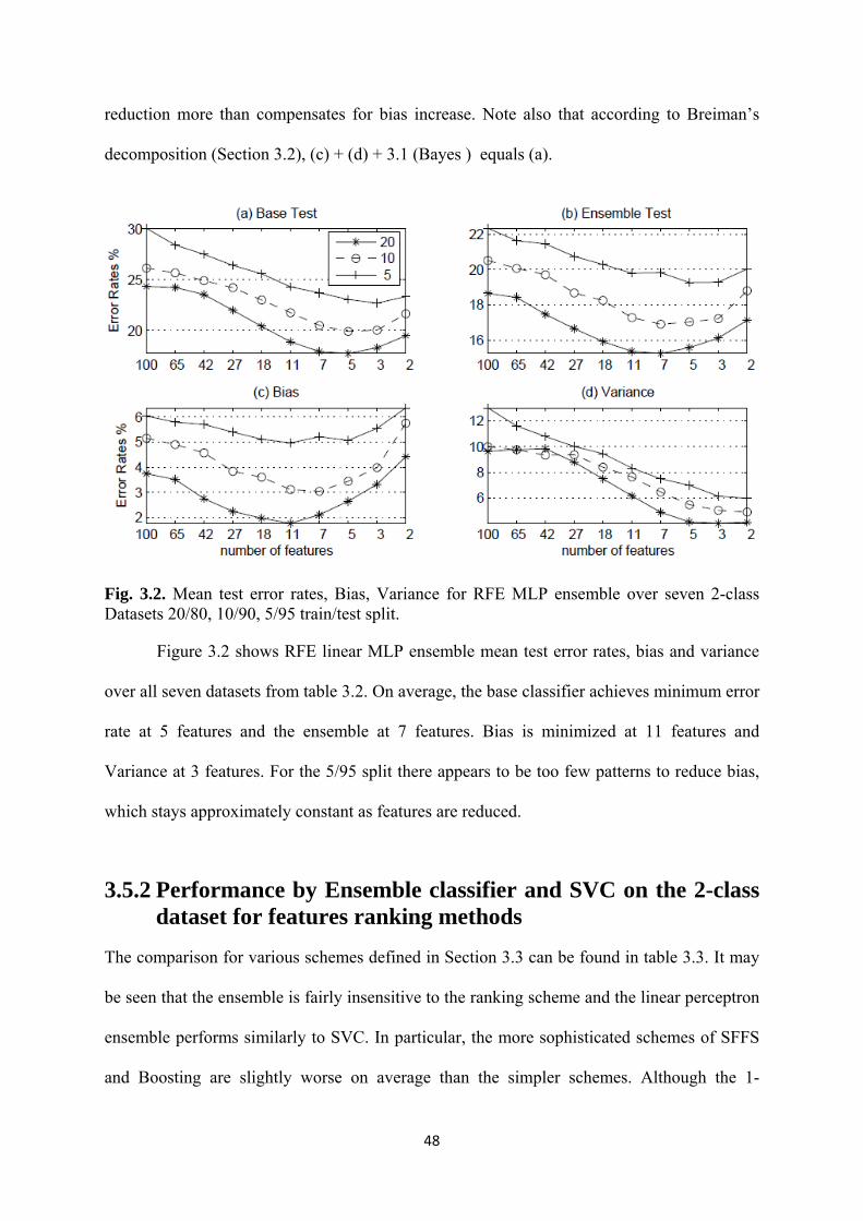
48  

reduction more than compensates for bias increase. Note also that according to Breiman’s

decomposition (Section 3.2), (c) + (d) + 3.1 (Bayes ) equals (a).

Fig. 3.2. Mean test error rates, Bias, Variance for RFE MLP ensemble over seven 2-class Datasets 20/80, 10/90, 5/95 train/test split.

Figure 3.2 shows RFE linear MLP ensemble mean test error rates, bias and variance

over all seven datasets from table 3.2. On average, the base classifier achieves minimum error

rate at 5 features and the ensemble at 7 features. Bias is minimized at 11 features and

Variance at 3 features. For the 5/95 split there appears to be too few patterns to reduce bias,

which stays approximately constant as features are reduced.

3.5.2 Performance by Ensemble classifier and SVC on the 2-class dataset for features ranking methods

The comparison for various schemes defined in Section 3.3 can be found in table 3.3. It may

be seen that the ensemble is fairly insensitive to the ranking scheme and the linear perceptron

ensemble performs similarly to SVC. In particular, the more sophisticated schemes of SFFS

and Boosting are slightly worse on average than the simpler schemes. Although the 1-

49  

dimensional method (Section 3.3.4) is best on average for 20/80 split, as number of training

patterns decreases, performance is slightly worse than RFE methods. MLP base classifier

with 8 nodes 7 epochs was also tried and it was found to be the best setting without added

noisy features [9]. The mean ensemble rate for 20/80, 10/90 5/95 was 14.5%, 15.7%, 17.9%

respectively, the improvement due mostly to ‘ion’ dataset which has a high bias with respect

to Bayes classifier.

Table 3.3. Mean best error rates (%)/number of features for seven two-class problems (20/80) with five feature-ranking schemes (Mean 10/90, 5/95 also shown).

perceptron-ensemble classifier SVC-classifier

rfenn rfenb 1dim SFFS boost rfesvc rfenb 1dim SFFS boost

diab 24.9/2 25.3/2 25.3/2 25.8/2 25.6/2 24.5/3 24.8/5 24.9/2 25.3/2 25.3/2

credita 16.5/5 15.7/3 14.6/2 15.6/2 15.5/2 15.7/2 15.1/2 14.6/2 15.4/2 15.1/2

cancer 4/7 4/5 4.1/5 4.4/3 4.9/7 3.7/7 3.7/7 3.8/11 4.2/5 4.5/7

heart 21/27 21/18 21/11 23/5 23/18 20/18 20/11 20/18 22/7 24/18

vote 5.5/5 5.3/7 5.6/18 5.7/2 5.5/2 4.8/2 4.8/2 4.7/2 4.3/3 4.7/2

ion 18/11 16.7/3 14.8/3 15.8/3 18.1/2 15/11 15.9/7 15.3/5 17.9/5 19.5/5

card 15.7/7 15/2 14.7/2 16.9/2 14.8/2 15.5/2 14.8/2 14.5/2 16.6/2 14.5/2

Mean20/80 15.1 14.6 14.2 15.4 15.4 14.2 14.2 13.9 15.1 15.3

Mean10/90 16.3 16.3 16.6 18.0 17.6 15.5 15.7 15.8 17.5 17.3

Mean5/95 18.4 18.5 20.0 21.3 21.3 17.0 17.7 18.4 20.3 20.7

To determine the potential effect of using a validation set with a feature selection

strategy, we chose SVC plus SFFS with the unrealistic case of full test set for tuning. The

mean ensemble rate for 20/80, 10/90 5/95 was 13.3%, 14.0%, 15.0% for SVC and 13.5%,

14.1%, 15.4% for MLP. We also repeated rfenn without Bootstrapping, showing that

although variance is lower, bias is higher and achieved 15.7%, 17.6%, 20.0% respectively,

demonstrating that Bootstrapping has beneficial effect on performance.

50  

3.5.3 Features ranked between Ensemble classifier and SVC on the face dataset

Table 3.4. Mean best error rates (%)/number of features for au1 classification 90/10 with five feature-ranking schemes.

MLP-ensemble classifier SVC-classifier

rfenn rfenb 1dim SFFS boost rfesvc rfenb 1dim SFFS boost

10.0/28 10.9/43 10.9/43 12.3/104 11.9/43 11.6/28 12.1/28 11.9/67 13.9/67 12.4/43

Table 3.4 shows feature-ranking comparison for au1 classification from the Cohn-

Kanade database as described in Section 3.4. It was found that lower test error was obtained

with non-linear base classifier and figure 3.3 shows test error rates, using an MLP ensemble

with 16 nodes 10 epochs. The minimum base error rate for 90/10 split is 16.5% achieved for

28 features, while the ensemble is 10.0% at 28 features. Note that for 50/50 split there are too

few training patterns for feature selection to have much effect. Since class distributions are

unbalanced, the overall error rate may be misleading, as explained in Section 3.4. Therefore,

we show the true positive rate in figure 3.3 c) and area under ROC in figure d).

Fig. 3.3. Mean test error rates, True Positive and area under ROC for RFE MLP ensemble for au1 classification 90/10, 50/50 train/test split.

51  

Note that only 71% of au1s are correctly recognized. However, by changing the threshold for

calculating the ROC, it is clearly possible to increase the true positive rate at the expense of

false negatives. SVC for degree 2,3,4 polynomials with varying C was also tried, but did not

improve on degree 1 results. It was observed that the performance of SVC was very sensitive

to regularization constant C, which makes it difficult to tune. In these experiments a linear

kernel was used.

Table 3.5. ECOC super-classes of action units and number of patterns.

Table 3.6. Mean best error rates (%) and area under ROC showing #nodes /#features for au classification 90/10 with optimized PCA features and MLP ensemble.

2-class Error %

2-class ROC

ECOC Error %

ECOC ROC

au1 8.0/16/28 0.97/16/36 9.0/4/36 0.94/4/17 au2 2.9/1/22 0.99/16/36 3.2/16/22 0.97/1/46 au4 8.5/16/36 0.95//16/28 9.0/1/28 0.95/4/36 au5 5.5/1/46 0.97/1/46 3.5/1/36 0.98/1/36 au6 10.3/4/36 0.94/4/28 12.5/4/28 0.92/1/28 au7 10.3/1/28 0.92/16/60 11.6/4/46 0.92/1/36 mean 7.6 0.96 8.1 0.95

Additionally experiments were performed using the ECOC method described in Section 3.2.

The ultimate goal in au classification is to detect combination of aus. In the ECOC approach,

a random 200×12 code matrix Z is used to consider each au combination as a different class.

After removing classes with less than four patterns this gives a 12-class problem with au

combinations as shown in table 3.5. To compare the results with 2-class classification, the

test error is computed by interpreting super-classes as 2-class problems, defined as either

containing or not containing respective au. For example, sc2, sc3, sc6, sc11, sc12 in table 3.5

are interpreted as au1, and remaining super-classes as non-au1. The last two columns of

ID sc1 sc2 sc3 sc4 sc5 sc6 sc7 sc8 sc9 sc10 sc11 sc12 superclass {} 1,2 1,2,5 4 6 1,4 1,4,7 4,7 4,6,7 6,7 1 1,2,4#patterns 149 21 44 26 64 18 10 39 16 7 6 4

52  

table 3.6 show ECOC classification error and area under ROC. This is compared with the

detection of aus using six different 2-class classification problems, where the second class

contains all patterns not containing respective au, using MLP ensemble with PCA feature

reduction. The results are in the first two columns of table 3.6 showing the best ensemble

error rate, number of features and number of nodes for all upper face aus. It may be seen that

2-class classification with optimized PCA features on average slightly outperforms ECOC.

However, the advantage of ECOC is that all problems are solved simultaneously with 200

classifiers, and furthermore the combination of aus is recognized. As a 12-class problem, the

mean best error rate over the twelve classes defined in table 3.5 is 38.2 %, achieved at 60

features with 1 node, showing that recognition of combination of aus is a difficult problem.

3.6 Conclusion

There is conflicting evidence over whether an SVC ensemble gives superior results compared

with single SVC, but in [107] it is claimed that an SVC ensemble with low bias classifiers

gives better results. However, it is not possible to be definitive, without searching over all

kernels and regularization constants C. In our experiments, we chose to consider only linear

SVC, and found the performance to be sensitive to C. In contrast, the ensemble is relatively

insensitive to number of nodes and epochs [9], and this is an advantage of the MLP ensemble.

However, it is likely that comparable results to MLP ensemble could have been achieved by

searching over different kernels and values of C for SVC.

A bootstrapped MLP ensemble, combined with RFE and product of weights feature-

ranking, is an effective way of eliminating irrelevant features. The accuracy is comparable to

SVC but has the advantage that the OOB estimate may be used to tune parameters and to

determine when to stop eliminating features. Simple feature-ranking techniques, such as 1-

dimensional class separability measure or product of MLP weights plus RFE, perform at least

53  

as well as more sophisticated techniques such as multi-dimensional methods of SFFS and

Boosting.

The feature-ranking approaches have been applied to a two-class problem in facial

action unit classification. The problem of detecting action units is naturally a multi-class

problem, but in this chapter this problem has been decomposed into two-class problems using

PCA and Error-Correcting Output Coding (ECOC) [91] approaches. For upper face aus

optimized 2-class classifiers give slightly lower mean error rates than ECOC. However,

ECOC can detect combinations of aus and further work is aimed at determining whether

problem-dependent rather than random ECOC codes can give better results.

In chapter 4, we use RFE as a pruning method for regression and consider other

dynamic pruning approaches.

 

 

   

54  

Chapter4

Dynamic Ensemble Selection and Instantaneous Pruning for Regression

A dynamic method of selecting a pruned ensemble of predictors for the

regression problem is described in this chapter. The method described enhances

the prediction accuracy and generalisation ability of the pruning methods that

change the order in which ensemble members are combined. Ordering heuristics

attempt to combine accurate yet complementary predictors. The proposed method

enhances the performance by modifying the order of aggregation through

distributing the ensemble selection over the entire dataset. Four static ensemble

pruning approaches have been compared with the proposed dynamic method

using Multi-Layer Perceptron predictors on publicly available benchmark

datasets.

4.1 Introduction

Ensemble pruning has been extensively investigated in the literature in the context of

ensemble methods. While it is recognised that combined outputs of several predictors

generally give improved accuracy compared to a single predictor [108] it has also been

shown that ensemble members that are complementary can be selected to further improve the

performance. This selection of ensemble members or ensemble pruning has the potential

advantage of both reduced ensemble size and improved accuracy. Predictors in the form of

classifiers, rather than regressors (continuous value predictors) have previously received

more attention and given rise to many approaches to pruning [71]. A categorisation of

different pruning methods for classifiers, including ranking-based, clustering-based and

optimisation based can be found in [108]. Some of these methods have been adapted to the

55  

regression problem [109] in both the static and dynamic form. In this chapter a dynamic

method of pruning is described, that can improve the performance of ranking-based methods.

In this method the subset of predictors is chosen differently depending on the test sample and

its relationship to the training set.

In general, an ensemble of predictors is constructed in two ways. First the component

members of the ensemble are trained and secondly the predictions are combined. In the

training of ensembles two approaches are widely used, namely Bagging and Boosting. Both

use re-sampling, but Bagging is a simpler method and introduces randomness into the

training process by sampling with replacement. Bagging is chosen here due to its robustness,

its ability to perform well on noisy data and its generalisation ability [109].

In this chapter a novel method of dynamic selection of pruned ensembles for

regression is presented. Initially ordering using Reduced Error method without Back Fitting

[71] is performed on the pool of predictors, generated by Bagging. This ordering is thus

based on the randomised bootstraps over the full training set and performed on every pattern

of the training set. This information is then archived for later retrieval for test patterns where

the ensemble order relating to the closest training pattern is retrieved. The output of the test

sample is generated by combining the output of the selected ensemble in the order specified.

4.2 Ensemble Pruning

In this chapter four static ensemble pruning methods have been investigated along with their

dynamic form to compare performances between static and dynamic ensemble methods.

These methods are classified as static methods, since they prune the ensemble once using

either a validation set or some other means where the performance of the pruned ensemble on

average yields the best performance for patterns not used for training. This ensemble with the

56  

selected members is then used for all the test patterns thenceforth. In contrast to static

methods, dynamic ensemble pruning selects ensemble members with a different selection for

every test pattern. Here again the selection scheme used may either take into account a

validation set to train a weight system allocated for the members that influences the ensemble

output or some other means to determine the suitability of the members to form the ensemble

for the test pattern. The dynamic approach helps to tailor the ensemble to the test pattern, so

that the performance of the ensemble is improved over the static methods. Therefore

generalisation and improved prediction accuracy of the ensemble may result from

dynamically selecting the ensemble members. Sections 4.3.1 – 4.3.4 describe the four static

methods used in this investigation to show the performance difference between the static

methods and novel dynamic ensemble pruning method.

4.2.1 Ordered Aggregation Pruning

Ordered Aggregation (OA) is a ranking-based pruning method where the order in which the

predictors are aggregated in a bagging ensemble is modified [71]. Before applying OA the

order is random, according to the different bootstrap samples of the original training data. For

random ordering, the prediction error as a function of ensemble size generally exhibits a

monotonic decrease approaching an asymptotic constant, which usually is the best obtainable.

By altering this order using some optimization criterion, a minimum in the error is achieved.

Figure 4.1 shows this reduction in the error as seen in the experimental evidence for MPL

based ensembles in this section. It is also observed that a minimum in the trained error is

reached with a fewer number of predictors in the ensemble.

57  

Fig. 4.1. Comparison of Ordered Aggregation Vs Random Ordered ensemble prediction error.

In [71] ordering based on minimizing a function Su (equation (4.1)) of the training error has

been suggested as the optimization criterion. This criterion specifies that from the initial pool

of M predictors generated by bootstrap samples, a nested ensemble of predictors are built, in

which the ensemble of size u contains the ensemble of size u-1 for aggregation. The

algorithm in [71] starts with an empty ensemble that grows by incorporating at each iteration

a predictor from M, without replacement, that minimizes Su which takes into account the

individual prediction accuracy and the complementarity of predictors, given by

1

1

)(1

1

)(1

1

)(2 2minargu

i

trkk

u

i

trks

u

j

trssku CCCus

iji (4.1)

where k ϵ (1,...,M)\{S1, S2,…,Su-1} and {S1, S2,…,Su-1} label predictors that have been

incorporated in the pruned ensemble at iteration u-1. In equation (4.1) Cii is the average

squared error of the ith ensemble member. The off diagonal term (Cij, i ≠ j) corresponds to the

correlation between the predictions of the ith and the jth ensemble members. Therefore this

average error is given by

2

4

6

8

10

12

14

16

18

20

0 5 10 15 20 25 30

Ordered Bagging

Bagging

Error

Ensemble Size Reduction

Number of Ensemble Members

Error Reduction

58  

N

nnnjnni

trij yxfyxf

NC

1

)( ))()()((1

(4.2)

where i = (1,2,…,M) and fi(x) is the prediction of the ith predictor, (xn ,yn) is the training data

where n = (1,2,…,N). Therefore the information required for the optimization of the training

error is contained in the matrix C(tr) in equation (4.2).

4.2.2 Recursive Feature Elimination Pruning

Recursive Feature Elimination (RFE) in classification removes the least performing or the

lowest ranked feature in order to improve the performance of the ensemble. As stated in

Section 3.3 RFE recursively ranks features according to a suitable feature-ranking method

and removes the least ranked features. Here the feature ranking strategy is based on the

weights of neural network classifiers. Extending this strategy to a trained combiner, the

weights of the trained combiner is used for ranking the ensemble members. In this method a

neural network is used as the trained combiner and trains using the outputs of the ensemble

member predictors as inputs to this neural network and the target values in the training set.

The trained combiner output O using a single output single hidden-layer Multiple Layer

Perceptron (MLP), assuming sigmoid activation function S is given by

j

ji

iji WWxSO 21 *)( (4.3)

where i,j are the input and hidden node indices, xi is an ensemble member output which is an

input to the trained combiner, W1 and W2 are first layer weight matrix and the output weight

vector respectively. From equation (4.3) a local input feature selection weight wi is derived in

equation (4.4) and this weight is considered as the rank attached to the ensemble member.

j

jiji WWw 21 * (4.4)

59  

To adapt the above derivation for the regression problem, the predictors in the

ensemble are ranked by training the trained combiner and then by evaluating the rank using

equation (4.4). The least relevant predictor is then identified and removed from the ensemble.

Then by iterating this process for the remaining predictors, RFE obtains the ranking for

pruning.

4.2.3 Pruning Optimisation Using Genetic Algorithms

Ensemble pruning by the application of Genetic Algorithm (GA) is based on a ranking

method. The idea of GA is that ensemble generalizing error can be optimized to achieve a

minimum by assuming that each predictor can be assigned a weight that could characterize

the fitness for the predictor to be included in the ensemble. In the regression problem the

weight associated with a predictor is a binary function, where a 1 indicates the inclusion of

the predictor in the ensemble. The variable of the weight function in GA that produces the

binary behavior is shown in equation (4.5).

)5.0(1

1

ivki e

w (4.5)

where wi ( i = 1,2,…M) is the weight and M is the number of predictors. vi is the variable in

GA associated with the ith predictor and k is the steepness function where this is set to 1000.

Equation (4.6) shows the required behavior of w(v).

5.0

5.0

0

1)(

v

vvw (4.6)

The ensemble generalization error E is given in equation (4.7)

60  

M

ii

M

i

trii

w

CwE

1

1

)(

(4.7)

N

nnni

tri yxf

NC

1

2)( ))((1

(4.8)

where i = (1,2,…,M) and fi(x) is the prediction of the ith predictor, (xn ,yn) is the training data

where n = (1,2,…,N). The GA minimizing function is given in equation (4.9)

10

0.

min

1

1

1

i

M

ii

M

ii

M

i

trii

v

wNts

w

Cw

v

(4.9)

4.2.4 Reduced Error Pruning

Reduced Error pruning (RE) without Back Fitting method [71], modified for regression

problems, is used to establish the order of predictors in the ensemble that produces a

minimum in the ensemble training error. Starting with the predictor that produces the lowest

training error, the remaining predictors are subsequently incorporated one at a time into the

ensemble to achieve a minimum ensemble error. The sub ensemble Su is constructed by

incorporating to Su-1 the predictor that minimizes

1

1

)()(1minargu

i

trk

trsku CCus

i (4.10)

where k ϵ (1,...,M)\{S1, S2,…,Su-1} and {S1, S2,…,Su-1} label predictors that have been

incorporated in the pruned ensemble at iteration u-1.

61  

N

nnni

tri yxf

NC

1

)( ))((1

(4.11)

where i = 1,2,…,M , fi(x) is the output of the ith predictor and (xn ,yn) is the training data

where n = (1,2,…,N). Therefore the information required for the optimization of the training

error is contained in the vector Ci(tr).

4.2.5 Dynamic Ensemble Pruning

Dynamic Ensemble Selection and Instantaneous Pruning (DESIP) is a novel ensemble

selection method introduced in this chapter and uses an ordering process by which the

ensemble members are ordered based on their performance. When training completes

producing the ensemble member predictors that constitute the ensemble, ordering these

ensemble members takes place on a pattern by pattern basis using the training set according

to the RE method. Therefore a different order of members will be formed for every pattern in

the training set, and with this ensemble pruning takes place for every pattern in the training

set where the members that aggregate the error to a minimum are selected and ordered. One

novel aspect of this method is the selection of sub-ensembles from the same pool of

predictors, where this selection is governed by the training set, giving rise to a map between

the training patterns and their order of selection of predictors. This mapping is archived for

the purpose of determining an ensemble predictor order for a test pattern during the test

phase. By searching the training set for a pattern that is closest to the test pattern, an

ensemble of predictors with the selection order defined by the searched training pattern is

retrieved from the archive. The predictor order thus found may not be the optimal order of

predictors for the test pattern, since the predictor order is of the training pattern that is close

to the test pattern based on a distance measure. Therefore having more training patterns in the

training set and thereby reducing the distance between patterns helps to increase the

62  

optimality of the predictor order. With the static methods, this distribution of the ensemble

order between training patterns does not occur, and therefore the optimality of the order is

fixed for the test pattern. Therefore the prediction accuracy is lower in the static methods in

comparison to DESIP.

The search carried out for determining the closest training pattern to the test pattern is

implemented with the distance as a measure of closeness. In this investigation K-Nearest

Neighbours (K-NN) method with L1 norm as the distance measure was selected for searching

for the closest training pattern. Therefore the second novel aspect of this method is that it

involves a search for the optimal predictor order as a function of the distance between the test

pattern and the patterns in the training set. Other distance measures, such as Mahalanobis

distance and Euclidean distance were also investigated. In DESIP all features or dimensions

of the data were considered in the K-NN search. However when using distance as the

measure of closeness between patterns, some features of the data may not be effective in the

calculation of the distance. This may be due to its irrelevance to the distance measure, giving

rise to redundant features. This effect has not been investigated in the test carried out and

would form a part of future work.

4.3 Method

In contrast to static ensemble selection, Dynamic Ensemble Selection with Instantaneous

Pruning (DESIP) provides an ensemble tailored to the specific test pattern based on the

information of the training set. The proposed method described here is for a regression

problem where the predictors are ordered for every individual training pattern based on the

method of RE. Therefore each ensemble selection for every training pattern contains the same

predictors as constituent members but aggregated in a different order. However, potentially

this dynamic method can be implemented with any pruning technique.

63  

The implementation of DESIP consists of two stages. First the base predictors M are

trained on bootstrap samples of the training dataset and the predictor order is found for every

pattern in the training set. As shown in the pseudo-code in figure 4.2, this is achieved by

building a series of nested ensembles, per training pattern, in which the ensemble of size u

contains the ensemble of size u-1. Taking a single pattern of the training set, the method starts

with an empty ensemble S, in step 2, and builds the ensemble order, in steps 6 to 15, by

evaluating the training error of each predictor in M. The predictor that increases the ensemble

training error least is iteratively added to S. This is achieved by minimizing z in step 9.

Therefore each predictor in M takes a unique position in S as S grows. This order is archived

in a two dimensional matrix A with predictor order in rows and training pattern in columns.

In the second stage, the predictor order that is associated with the training pattern

closest to the test pattern is retrieved from matrix A. Here the closeness is determined by

calculating the L1 Norm of the distance measure between the test pattern and the training set.

This is performed in steps 1 to 5 in figure 4.3. All input features of the training set are

considered to identify the closest training pattern, using the K-Nearest Neighbors method

[115], where K = 1. The resulting vector gn, where n is the index of the training pattern, is

searched for the minimum value and is identified as the closest training pattern to be retrieved

from A. The selected ensemble has the order of predictors determined by the training pattern.

For the comparison of DESIP with static methods, four static pruning methods were

implemented with DESIP. They are Ordered Aggregation (OA) as described in [71] for

regression, Recursive Feature Elimination (RFE) in [114], ensemble optimization using

Genetic Algorithm (GA) and Reduced Error Pruning without Back Fitting (RE) [70].

64  

Fig. 4.2. Pseudo-code implementing the archive matrix with ordered ensemble per training data.

Fig. 4.3. Pseudo-code implementing the identification of the nearest training pattern to the test pattern.

Training data D = (xn, yn), where n = (1, 2,.., N) and fm  is a predictor,  

where m = (1, 2,.., M). The Archive Matrix  A = (an ) where an is a column vector with max index of m. S is also a vector with max index of m. 

1.  For n = 1….N 2.       S  empty vector 3.      For m = 1…M 4.         Evaluate   

nnmm yxfC )(  

5.       End for 6.       For u = 1…M 7.        min    +∞ 8.         For k in (1,…, M)\{S1, S2,…, Su} 

9.           Evaluate   

1

1

1u

ikS CCuz

i 

10.           If  z < min 11.             Su    k 12.             min    z 13.           End if 14.         End for 15.       End for 16.       an  S 17.   End for 

Test and train pattern xf,test, xf,n,train where f = (1, 2,.., F) features.  From figure 4.1 Archive Matrix  A = (an) where an is the column vector containing the order of predictors, n = 1, 2,.., N. ef is a vector with max index of F and gn is a vector with max index of N. 1.  For n = 1….N 2.       For f = 1….F 3.       Evaluate ef = |xf,n,train ‐ xf,test| 4.       End for 5.  End for 6.  Search for the minimum values in gn and note n 7.  an is the ensemble selection for the test pattern. 

65  

4.4 Experimental Evidence

In this section the results of the four ensemble selection methods applied to benchmark

datasets are presented. These datasets were selected since they contain continuous value

outputs (regression). Based on preliminary experiments, an MLP architecture with 5 nodes in

the hidden layer has been selected in this experiment to train the ensemble of base predictors.

The training/test data split is 70/30 percent, and bootstrap samples for 32 base predictors are

trained. The Mean Squared Error (MSE) is used as the performance indicator for both

training set and test set, and an average is obtained over 100 iterations.

Table 4.1 lists the publicly available bench mark datasets [116] and [117] used in

these experiments and figure 4.4 shows train and test MSE versus sub-ensemble size of these

datasets. It can be observed from figure 4.4 that the MSE of the dynamic method for the

training set is significantly lower than the static methods, indicating that the individual

ensembles selected based on the training set have been optimized. In the MSE plots of the

test set in figure 4.4, the apparent optimal solution of the problem has been achieved by the

proposed dynamic method. It is also observed that the minimum occurs at a lower ensemble

size with the dynamic selection method than the static methods.

Table 4.1. Benchmark datasets used for experiments showing the number of patterns and features.

Dataset Patterns Features Source Servo 167 5 UCI-Repository Boston Housing 506 14 UCI-Repository Forest Fires 517 14 UCI-Repository Wisconsin 198 36 UCI-Repository Concrete Slump 103 8 UCI-Repository Auto93 82 20 WEKA Auto Price 159 16 WEKA Body Fat 252 15 WEKA Bolts 40 8 WEKA Pollution 60 16 WEKA Sensory 576 12 WEKA

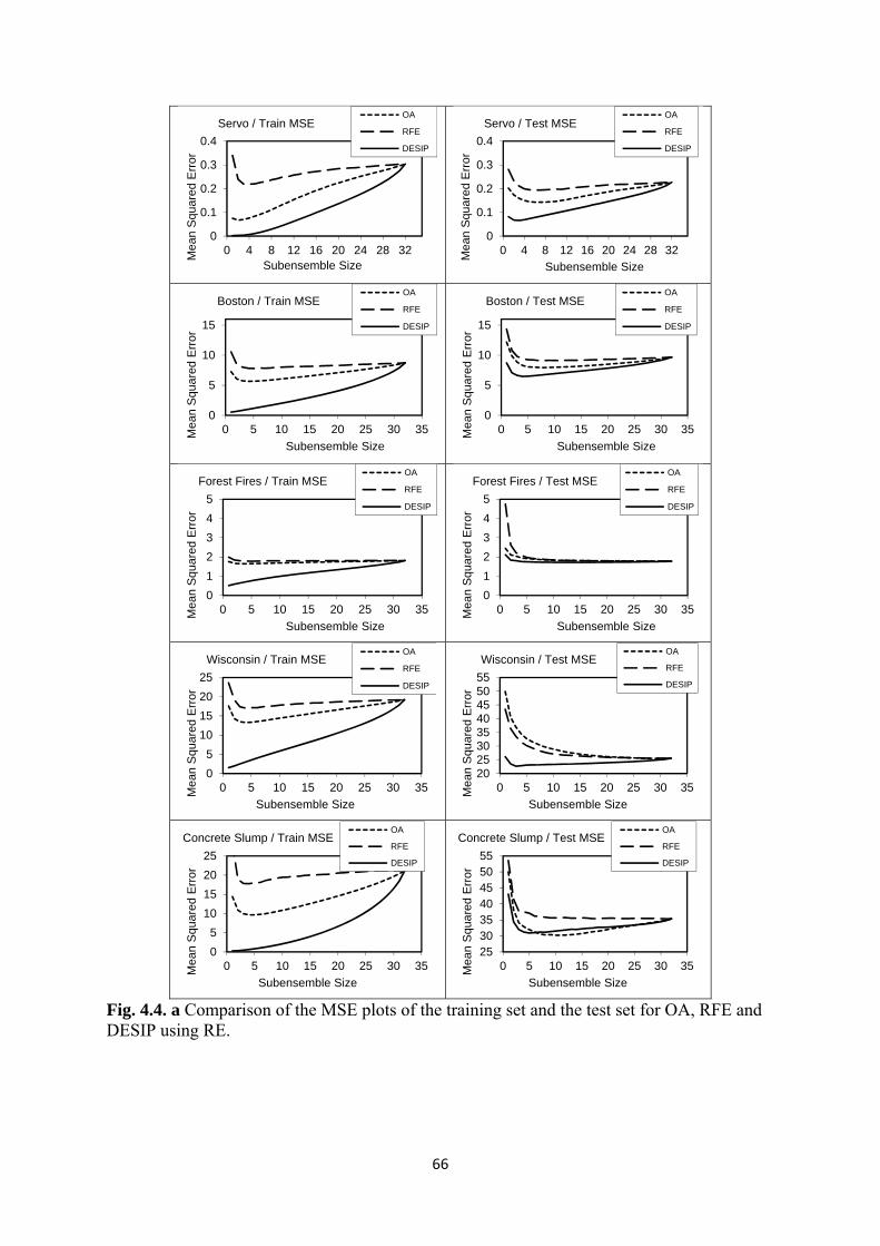
66  

 

 

 

 

 

Fig. 4.4. a Comparison of the MSE plots of the training set and the test set for OA, RFE and DESIP using RE.

 

 

0

0.1

0.2

0.3

0.4

0 4 8 12 16 20 24 28 32Mea

n S

quar

ed E

rror

Subensemble Size

Servo / Train MSEOA

RFE

DESIP

0

0.1

0.2

0.3

0.4

0 4 8 12 16 20 24 28 32Mea

n S

quar

ed E

rror

Subensemble Size

Servo / Test MSEOA

RFE

DESIP

0

5

10

15

0 5 10 15 20 25 30 35Mea

n S

quar

ed E

rror

Subensemble Size

Boston / Train MSEOA

RFE

DESIP

0

5

10

15

0 5 10 15 20 25 30 35Mea

n S

quar

ed E

rror

Subensemble Size

Boston / Test MSEOA

RFE

DESIP

0

1

2

3

4

5

0 5 10 15 20 25 30 35Mea

n S

quar

ed E

rror

Subensemble Size

Forest Fires / Train MSEOA

RFE

DESIP

0

1

2

3

4

5

0 5 10 15 20 25 30 35Mea

n S

quar

ed E

rror

Subensemble Size

Forest Fires / Test MSEOA

RFE

DESIP

0

5

10

15

20

25

0 5 10 15 20 25 30 35Mea

n S

quar

ed E

rror

Subensemble Size

Wisconsin / Train MSEOA

RFE

DESIP

2025303540455055

0 5 10 15 20 25 30 35Mea

n S

quar

ed E

rror

Subensemble Size

Wisconsin / Test MSEOA

RFE

DESIP

0

5

10

15

20

25

0 5 10 15 20 25 30 35Mea

n S

quar

ed E

rror

Subensemble Size

Concrete Slump / Train MSEOA

RFE

DESIP

25303540455055

0 5 10 15 20 25 30 35Mea

n S

quar

ed E

rror

Subensemble Size

Concrete Slump / Test MSEOA

RFE

DESIP

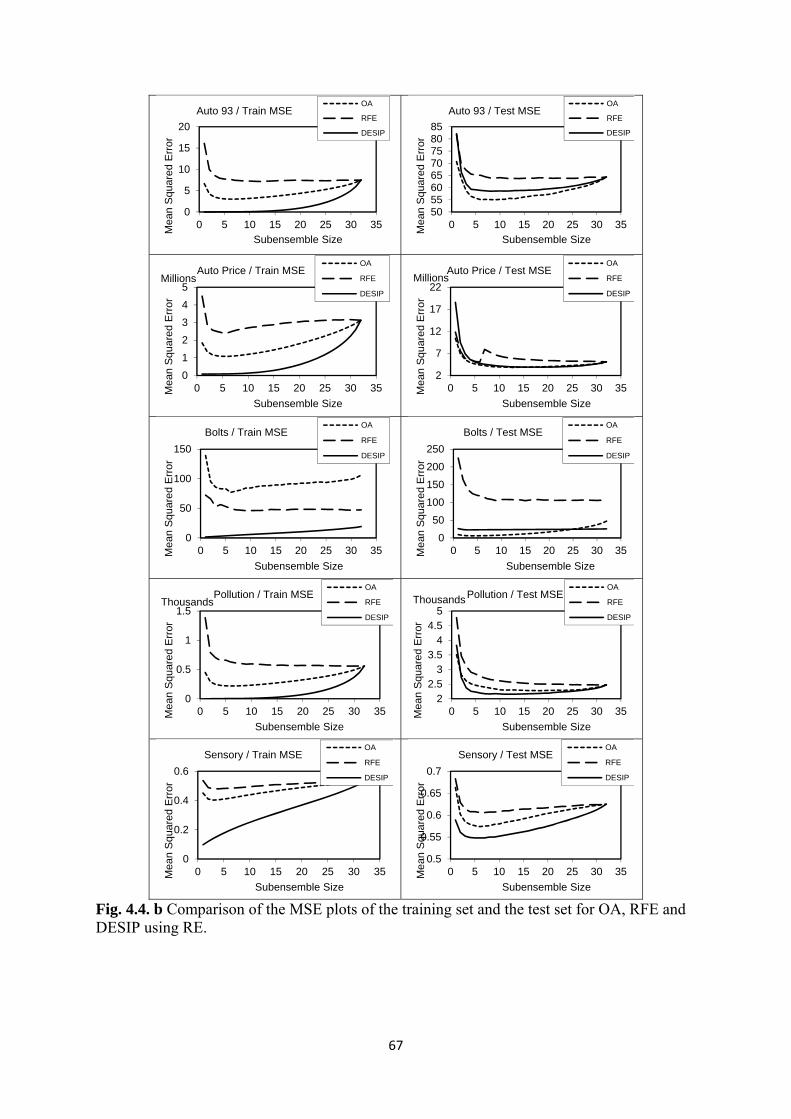
67  

   

 

 

 

 Fig. 4.4. b Comparison of the MSE plots of the training set and the test set for OA, RFE and DESIP using RE.

 

 

0

5

10

15

20

0 5 10 15 20 25 30 35Mea

n S

quar

ed E

rror

Subensemble Size

Auto 93 / Train MSEOA

RFE

DESIP

5055606570758085

0 5 10 15 20 25 30 35Mea

n S

quar

ed E

rror

Subensemble Size

Auto 93 / Test MSEOA

RFE

DESIP

0

1

2

3

4

5

0 5 10 15 20 25 30 35Mea

n S

quar

ed E

rror

Millions

Subensemble Size

Auto Price / Train MSEOA

RFE

DESIP

2

7

12

17

22

0 5 10 15 20 25 30 35Mea

n S

quar

ed E

rror

Millions

Subensemble Size

Auto Price / Test MSEOA

RFE

DESIP

0

50

100

150

0 5 10 15 20 25 30 35Mea

n S

quar

ed E

rror

Subensemble Size

Bolts / Train MSEOA

RFE

DESIP

0

50

100

150

200

250

0 5 10 15 20 25 30 35Mea

n S

quar

ed E

rror

Subensemble Size

Bolts / Test MSEOA

RFE

DESIP

0

0.5

1

1.5

0 5 10 15 20 25 30 35Mea

n S

quar

ed E

rror

Thousands

Subensemble Size

Pollution / Train MSEOA

RFE

DESIP

22.5

33.5

44.5

5

0 5 10 15 20 25 30 35Mea

n S

quar

ed E

rror

Thousands

Subensemble Size

Pollution / Test MSEOA

RFE

DESIP

0

0.2

0.4

0.6

0 5 10 15 20 25 30 35Mea

n S

quar

ed E

rror

Subensemble Size

Sensory / Train MSEOA

RFE

DESIP

0.5

0.55

0.6

0.65

0.7

0 5 10 15 20 25 30 35Mea

n S

quar

ed E

rror

Subensemble Size

Sensory / Test MSEOA

RFE

DESIP

68  

4.4.1 Performance variation between Static Pruning methods and the proposed Dynamic Pruning method

Table 4.2 shows the MSE performance of the four static methods, while table 4.3 shows static

methods implemented in DESIP. In table 4.2 and 4.3, grayed results indicate the minimum

MSE over the eight methods. It is observed that the majority of the lowest MSE values have

been achieved by DESIP. Table 4.4 shows the average ensemble size of each dataset for the

four static methods and their dynamic methods. It also shows the overall average ensemble

size per static method and their dynamic form.

Table 4.2. Static Ensemble Pruning Methods: Averaged MSE with Standard Deviation for the 100 iterations.

Dataset Multiplier OA RFE GA RE Servo 10-1 1.43±0.40 1.94±0.50 2.37±0.4 1.42±0.24 Boston Housing 100 7.94±0.60 9.12±0.94 9.91±0.83 7.97±0.64 Forest Fires 100 1.78±0.05 1.78±0.08 1.81±0.18 1.78±0.07 Wisconsin 101 2.54±0.10 2.55±0.10 2.58±0.17 2.53±0.12 Concrete Slump 101 3.02±0.16 3.54±0.26 3.66±0.39 2.89±0.36 Auto93 101 5.50±0.81 6.37±0.77 6.52±0.66 5.58±0.93 Auto Price 106 3.81±0.64 5.04±1.89 6.09±8.03 3.88±0.63 Body Fat 10-1 6.91±1.23 6.80±6.70 8.44±2.81 5.99±2.12 Bolts 101 7.70±3.90 10.50±3.71 10.95±3.71 7.81±4.69 Pollution 103 2.28±0.22 2.47±0.22 2.54±0.31 2.26±0.21 Sensory 10-1 8.70±0.30 6.10±0.20 6.29±0.19 5.73±0.26

Table 4.3. DESIP with Static Methods Adopted: Averaged MSE with Standard Deviation for the 100 iterations.

Dataset Multiplier OA RFE GA RE Servo 10-1 0.66±0.21 1.46±0.43 1.35±0.30 0.66±0.21 Boston Housing 100 6.47±0.78 8.70±0.86 8.06±0.77 6.47±0.78 Forest Fires 100 1.72±0.08 1.76±0.10 1.79±0.76 1.72±0.09 Wisconsin 101 2.27±0.28 2.29±0.08 2.18±0.14 2.27±0.28 Concrete Slump 101 3.09±0.56 3.16±0.23 3.14±0.39 3.09±0.56 Auto93 101 5.85±0.83 6.35±0.81 6.51±0.67 5.85±0.83 Auto Price 106 3.88±0.63 5.16±2.13 5.85±4.59 3.88±0.63 Body Fat 10-1 6.12±1.57 6.17±3.10 5.96±1.50 6.12±1.57 Bolts 101 7.44±2.43 7.42±2.82 7.33±2.55 7.44±2.43 Pollution 103 2.15±0.26 2.30±0.19 2.35±0.30 2.15±0.26 Sensory 10-1 5.48±0.16 5.85±0.13 6.11±0.20 5.48±0.16

 

69  

Table 4.4. Comparison of the minimum average ensemble size: Static Method / DESIP with Static Method Adopted. 

Dataset OA/DESIP RFE/DESIP GA/DESIP RE/DESIP Servo 7/2 5/4 15/12 7/2 Boston Housing 7/3 7/5 16/11 8/3 Forest Fires 15/15 32/15 15/8 30/13 Wisconsin 29/2 31/15 17/11 24/2 Concrete Slump 9/4 31/12 15/11 8/4 Auto93 8/7 11/9 16/14 6/7 Auto Price 12/15 5/5 16/13 11/15 Body Fat 28/13 23/10 16/16 4/5 Bolts 5/12 14/14 15/15 3/2 Pollution 17/10 29/15 16/13 17/10 Sensory 5/5 6/5 14/9 5/5 Average 13/8 18/10 16/12 11/6

4.4.2 Performance variation of pruning with different distance measures

The investigation further makes a comparison into the different distance measures of the K-

NN search for the closest pattern in the training set to the test pattern. The MSE performance

of these distance measures are shown in tables 4.5 and 4.6. Tables 4.5. and 4.6 show the

average MSE performance of different distance measures used with DESIP, namely

Eucledian and Mahalanobis distance. Here also a comparison is drawn between the pruning

methods applied to DESIP.

Table 4.5. Averaged MSE of DESIP – Using Euclidean distance. Dataset Multiplier OA RFE GA RE Servo 10-1 1.42±0.22 2.85±0.68 2.36±0.51 1.42±0.22 Boston Housing 100 8.71±0.68 10.36±0.42 10.09±1.33 8.71±0.68 Forest Fires 100 1.77±0.04 1.81±0.14 1.82±0.29 1.77±0.04 Wisconsin 101 2.48±0.12 2.85±0.23 2.64±0.32 2.48±0.12 Concrete Slump 101 3.53±0.26 3.72±0.81 3.67±0.57 3.53±0.26 Auto93 101 5.91±0.52 6.42±0.88 6.48±0.94 5.91±0.52 Auto Price 106 3.95±0.73 5.73±1.32 5.84±3.28 3.95±0.73 Body Fat 10-1 6.30±1.32 8.93±1.52 8.79±2.66 6.31±1.32 Bolts 101 9.61±2.36 10.12±1.98 11.36±3.81 9.61±2.36 Pollution 103 2.24±0.21 2.36±0.32 2.61±0.55 2.24±0.21 Sensory 10-1 6.06±0.13 6.18±0.59 6.27±0.66 6.06±0.13

70  

Table 4.6. Averaged MSE of DESIP – Using Mahalanobis distance. Dataset Multiplier OA RFE GA RE Servo 10-1 1.96±0.4 2.87±0.56 2.33±0.42 1.96±0.4 Boston Housing 100 9.51±0.58 10.55±0.83 10.02±1.41 9.51±0.58 Forest Fires 100 1.78±0.07 1.80±0.06 1.82±0.23 1.78±0.07 Wisconsin 101 2.51±0.11 2.87±0.18 2.63±0.32 2.51±0.11 Concrete Slump 101 3.43±0.31 3.83±0.54 3.71±0.58 3.43±0.31 Auto93 101 6.27±0.88 6.44±0.58 6.57±0.98 6.27±0.88 Auto Price 106 3.98±0.77 5.37±0.83 5.49±1.39 3.98±0.77 Body Fat 10-1 6.61±1.27 8.88±1.61 8.73±2.68 6.61±1.27 Bolts 101 9.71±2.73 10.32±2.57 11.3±3.55 9.71±2.73 Pollution 103 2.33±0.02 2.38±0.28 2.53±0.41 2.33±0.02 Sensory 10-1 6.25±0.14 6.27±0.54 6.29±0.64 6.25±0.14

4.5 Conclusion

Dynamic ensemble pruning utilizes a distributed approach to ensemble selection and is an

active area of research for both classification and regression problems. In this chapter, a novel

method of dynamic pruning of regression ensembles is proposed. Experimental results show

that test error has been reduced by modifying the pruning based on the closest training

pattern. On a few datasets the proposed method using the L1 norm has not improved

performance and this would be an investigation for future work. The performance

comparison between using Euclidean distance and the Mahalanobis distance shows

comparable results. However in addition to these two distance measures other distance

measures would have to be investigated along with the value of K in K-Nearest Neighbors

method. In the experiments shown in this chapter the value of K is one, and as future work

values greater than one would show the variation of the performance based on K. The effect

of selecting relevant features in the dataset for the distance measure is also an area of interest

for future work. Bias/Variance and time complexity analysis should also help to understand

the performance relative to other static and dynamic pruning methods with similar

complexity.

71  

The approach taken for training ensemble members in DESIP has been epoch based,

where the back propagation rule has been applied after the average error of an entire epoch of

the training set has been calculated. Therefore after initializing the weights with random

values, each predictor is trained in the same manner. In this training regime all the patterns in

the training set collectively contribute to the weight adjustment. However a predictor may not

train well on all the patterns in the training set. Therefore the prediction accuracy of a

predictor may be less for some sections of the problem. The implication is that predictors of

an ensemble may be selectively trained on the patterns of the training set. This is investigated

in chapter 5 where the predictors of the ensemble are selectively trained based on their

aggregated performance on every patter individually. Here again ordering heuristics have

been used to determine which predictors are chosen for training.

 

   

72  

Chapter5

Hybrid Dynamic Learning Systems for Regression

Methods of introducing diversity into ensemble learning predictors for

regression are presented in this chapter. Here two methods are proposed, one

involving pruning and the other a hybrid approach. In these ensemble learning

approaches, diversity is introduced while simultaneously training, as part of the

same learning process. Here not all members of the ensemble are trained in the

same manner, but selectively trained, resulting in a diverse selection of

predictors that have strengths in different parts of the training set. The result is

that the prediction accuracy and generalization ability of the trained ensemble is

enhanced. Pruning and hybrid heuristics attempt to combine accurate yet

complementary members; therefore these methods enhance the performance by

dynamically modifying the pruned aggregation through distributing the ensemble

predictor selection over the entire dataset. A comparison is drawn with Negative

Correlation Learning and a static ensemble pruning approach used in regression

to highlight the performance improvement yielded by the dynamic methods.

Experimental comparison is made using Multiple Layer Perceptron predictors on

benchmark datasets.

5.1 Introduction

Diversity or heterogeneity among predictors enables the ensemble to compensate individual

errors and reach better expected performance. Therefore an important aspect of ensemble

creation is the injection of diversity into the individual predictors of the ensemble. Bagging

and Boosting are two popular methods used to date that achieve this objective. In Bagging

diverse predictors are generated by training with different sets of samples from a pool of

73  

training samples with replacement. In Boosting training samples are rated based on the

predictor’s performance on them and the low performing samples are given a higher rating so

that they are selected for training subsequent predictors. Like Bagging and Boosting, many

methods have emerged that incorporate diversity in some form into the predictors and the

characterisation of these methods suggests that the field has matured and therefore this

concept is regarded as an important element for performance improvement in ensemble

methods [118]. In this chapter we propose two learning methods that diversify the predictors.

The first proposed dynamic method, Ensemble Learning with Dynamic Ordered

Pruning (ELDOP) for regression, uses the Reduced Error (RE) pruning method without Back

Fitting (Section 4.3.4) for selecting the diverse members in the ensemble and only these are

used for training [61].

The second method, Hybrid Ensemble Learning with Dynamic Ordered Selection

(HELDOS), also uses the same RE method to select diverse members, but the ensemble is

split into two sub ensembles, of which one contains the most diverse members and other less

diverse. The most diverse members are then trained using Negative Correlation Learning

(NCL) method [67] while the less diverse members are trained independently. Here again the

selection and training of ensemble members are performed for every pattern in the training

set.

In chapter 4, by dynamic, we mean that the subset of predictors is chosen differently

depending on its performance on the test sample. In ELDOP, given that only selected

members of the ensemble are allowed to train for a given training pattern, the assumption is

made that only a subset of the ensemble will perform well on a test sample. Therefore the

method aims to automatically harness the ensemble diversity as a part of ensemble training.

ELDOP is novel, since pruning occurs with training, and unlike [119] [120], in the test phase

74  

there is no need to search for the closest training pattern. HELDOS harnesses diversity by

training the ensemble members differently for a given training pattern. Training a subset of

the ensemble using NCL, which relies on the correlation among the members of the sub-

ensemble, and the rest independently, introduces variation into the way the members are

trained. It is also assumed that a subset of the ensemble will perform well on a test sample.

The novelty in HELDOS is due to its simultaneous training with varied training methods.

In contrast to ELDOP, HELDOS trains all members in the ensemble for a given

training pattern. Therefore, for an epoch of training, a member is trained with varying number

of times by the two methods. All members in the HELDOS method are trained equal number

of times since all the members are trained for all the patterns in the training set. Whereas the

number of times a member is trained in the ELDOP method, can vary from one to all pattern

in an epoch. This is due to its member selection by ordering the members based on the RE

method and selecting a certain percentage of the members for training. With this a member

can be considered a strong or a weak predictor in different parts of the problem. This can

contribute to the generalization ability of the member predictors. Therefore diversity by

means of the training rate is introduced in this paper.

5.2 Pruning and Hybrid Learning

As shown by the Negative Correlation Learning (NCL) algorithm, diversity can be

encouraged by the learning method of ensemble predictors. As shown in chapter 4 Pruning

also provides an advantage in the diversification of ensembles where, when predictors are

selected dynamically on a pattern by pattern basis, a different ensemble of predictors is

chosen that helps to reduce the error. Therefore in this chapter the emphasis is on the learning

methods of ensemble predictors that can alter the ensemble selection in order to diversify

ensemble predictors. With this the methods investigated in this chapter try to obtain diverse

75  

predictors by training in different parts of the training space. As a consequence of training the

predictors in this manner it is expected that in the test phase predictor outputs that are in

agreement with each other will cluster together.

In the methods described in this chapter, the predictor selection is based on the

ordered ensemble of predictors, where the Reduced Error Pruning (RE) method without Back

Fitting is used for determining the order of the predictors according to their performance. RE

is described in section 4.3.4.

5.2.1 Ensemble Learning with Dynamic Ordered Pruning

In ELDOP pruning is carried out by selecting a certain percentage of the predictors with the

lowest error. Using RE the predictors are ordered on a pattern by pattern basis and trained

using the Back Propagation update rule. Therefore equation (4.11) in chapter 4 is modified to

express the error term used for the individual predictor and the individual pattern as follows.

(5.3)

where i = (1,2,…,M) , the function is the output of the ith predictor and (xn ,yn) is the

training data where n = (1,2,…,N) patterns. Therefore the information required for the

ordering of the training error is contained in the vector C. Using this error vector and the

equation (4.10) in chapter 4, the predictors are ordered and a portion of predictors with the

least error are selected using the following function to be trained.

(5.4)

where 1if ∈

0 otherwise

is defined as 50% of predictors with the lowest error, according to RE.

76  

5.2.2 Hybrid Ensemble Learning with Dynamic Ordered Pruning

Negative Correlation Learning (NCL) attempts to train and combine individual predictors in

the same learning process. In NCL all the individual outputs are trained simultaneously

through the correlation penalty terms in their error functions. The error function of an

individual predictor contains the empirical risk function, which is the general error of the

predictor, and the correlation penalty term. In NCL [67] the error term for the ith predictor for

the nth pattern is expressed as

1 (5.5)

where is the mean output of the selected predictors of the ensemble contributing

towards NCL and is the parameter 0 1 that is used to adjust the strength for the

penalty term. The value of in the experiments have been set to 1, so that equation (5.5)

becomes

(5.6)

In the hybrid method after ordering the predictors using the RE method described in

section 4.3.4, the ensemble members are split into two sub-ensembles. One sub-ensemble is

trained using NCL, while the second is trained using the Back Propagation update rule. To

accommodate the selection and training with the respective methods, equation (5.5) is

modified to the following

1 (5.7)

where 1if ∈

0 otherwise

is defined as 50% of predictors with the lowest error, according to RE.

77  

5.3 Methods

5.3.1 ELDOP

Dynamic selection of ensemble members provides an ensemble tailored to the specific test

instance. The method described here is for a regression problem where the ensemble

members are simultaneously ordered and trained on a pattern by pattern basis. The ordering

of ensemble members is based on the method of RE and only the first 50% of the ordered

members for a given training pattern are used for learning. Therefore diversity is encouraged

by training half of the ensemble members that perform well. The training continues until a

pre-determined number of epochs of the training set are completed.

Fig. 5.1. Pseudo-code implementing the training process with ordered ensemble pruning per training pattern for the ELDOP method.

Training data D = (xn, yn), where n = (1,2,..,N) and fm  is an ensemble member, where m = (1,2,..,M). S is a vector with max index of m. 

1. For n = 1….N 2.        S  empty vector 3.       For m = 1…M 4.          Evaluate  

nnmm yxfC )(  

5.        End for 6.        For u = 1…M 

7.         min    +∞ 8.          For k in (1,...,M)\{S1, S2,…,Su} 

9.            Evaluate  

1

1

1u

ikS CCuz

i 

10.          If  z < min 11.            Su   k 12.            min   z 13.          End if 14.        End for 15.     End for 16.       

where   1if ∈  0  otherwise 

 is 50% of predictors with the lowest error. 17.  End for 

78  

The implementation of ELDOP method consists of two stages. First the base ensemble

members M are ordered and trained on a pattern by pattern basis. As shown in the pseudo-

code in figure 5.1, this is achieved by building a series of nested ensembles in which the

ensemble of size u contains the ensemble of size u-1. Taking a single pattern of the training

set, the method starts with an empty ensemble S, in step 2, and builds the ensemble order, in

steps 6 to 15, by evaluating the training error of each predictor in M. The predictor that

increases the ensemble training error least is iteratively added to S. This is achieved by

minimizing z in step 9. Then the update rule is applied to the first 50% of the ordered

ensemble member in S (step 16). Therefore in one epoch of training, the Back Propagation

update rule would be applied a different number of times for each predictor, the more

effective predictors being trained the most.

In the second stage, the ensemble output for each test pattern is evaluated. The

assumption is made that the outputs of ensemble members that perform well for a test pattern

would cluster together. Therefore the second stage starts by clustering the ensemble outputs

into two clusters, which is shown in step 1 in figure 5.2. In step 2, the mean and the standard

deviation are calculated. Taking the ensemble member outputs of each cluster, the outputs

that are within one standard deviation from the mean are selected for the sub-cluster of each

original cluster. This is denoted by Sk, and shown in steps 5 to 9. Finally the mean of each of

these sub-clusters is calculated as the outputs of the original clusters (step 10).

79  

Fig. 5.2. Pseudo-code implementing the ensemble output evaluation for test pattern.

5.3.2 HELDOS

HELDOS also provides an ensemble tailored to the specific test instance, for the regression

problem. The ensemble members are simultaneously ordered and trained on a pattern by

pattern basis. The ordering of ensemble members is based on the method of RE and the first

50% of the ordered members are trained using the NCL method and the rest are trained

independently. Therefore diversity is encouraged by training subsets of the ensemble

members with differing methods. The training continues until a pre-determined number of

epochs of the training set is completed.

The implementation of HELDOS method also consists of two stages where the base

ensemble members M are ordered and trained on a pattern by pattern basis. This is achieved

by building a series of nested ensembles in which the ensemble of size u contains the

ensemble of size u-1. This is shown in the pseudo code in figure 5.3, from steps 2 to 15. Here

the predictor that increases the ensemble training error least is iteratively added to S. Taking a

Ensemble member output for a test pattern (xn, yn) is fm, where m = (1,2,..,M).  

fj  are ensemble member outputs in cluster Ck , j = 1,2,..,J number of members. 

,  are the mean and the standard deviation of Ck  

Sk is the sub‐cluster in Ck 

1. Using K‐means (K = 2) separate fm into two clusters C1 , C2 2. Find mean and standard deviation of the two clusters;  ,  ,  ,  , 3. Calculate cluster mean as follows for each of the two clusters C1 , C2: 4. For k = 1,2 5.      For j = 1….J 6.       If   fj  >   7.        Then  Sk  fj 8.       End if 9.      End for 10.    Evaluate  the mean of Sk ;  ̿ (This is the cluster output for comparison) 11. End for 

80  

single pattern of the training set the ensemble order of M predictors is thus built and using

this order the ensemble is split into two equal sub-ensembles (step 16). The first 50% of the

ensemble members in S are trained using the Negative Correlation Learning method using

equation (5.7). The second 50% of the ensemble members are trained independently using

the Back Propagation update rule on their individual errors. Therefore in one epoch of

training, the Negative Correlation Learning and Back Propagation update rule would be

applied a different number of times for each predictor.

Fig. 5.3. Pseudo-code implementing the training process with ordered ensemble pruning per training pattern for the HELDOS method.

The second stage of this method follows the same process described in ELDOP. The

ensemble output for each test pattern is evaluated and based on the assumption that outputs of

the ensemble members that perform well cluster together, the second stage starts by

clustering the ensemble outputs into two clusters. This is shown in step 1 in figure 5.2. In step

2, the mean and the standard deviation are calculated. The ensemble member outputs that are

within one standard deviation from the mean are selected for the sub-cluster of each original

cluster. This is denoted by Sk, and shown in steps 5 to 9. Finally the mean of each of these

sub-clusters is calculated as the outputs of the original clusters, as shown in step 10.

All steps, except step 16 from Figure 5.1 are applicable in this pseudo‐code block. Only equation of step 16 is shown here.  

16.     1  where   1if ∈  

0  otherwise  is 50% of predictors with the lowest error. 

81  

5.4 Experimental Evidence

The investigation of dynamic pruning is continued with experiments performed to study the

effects of incorporating pruning in the learning process and the publicly available benchmark

datasets [116] and [117] shown in table 5.1 have been used for the performance comparison.

Neural Networks with Multi-Layer Perceptron (MLP) architecture with 5 nodes in the hidden

layer as described in Section (4.5) has been selected in this experiment. The training and test

pattern split is 70% and 30% respectively. In this experiment 32 base predictors are trained

with identical training samples – i.e. without bootstrap sampling. This is to avoid the

diversity being introduced by random selections of the training patterns. The Mean Squared

Error (MSE) is used as the performance indicator for both training and test sets, and averaged

over 10 iterations. Training is stopped after fifty epochs.

Table. 5.1. Benchmark datasets used for experiments showing the number of patterns and features.

Table. 5.2. Averaged MSE of the test set with Standard Deviation for 10 iterations for NCL, OA, DESIP, ELDOP and HELDOS.

Dataset Multiplier NCL OA DESIP ELDOP HELDOS Servo 100 0.25±0.49 1.35±1.69 0.14±0.24 0.10±0.14 0.21±0.46 Wisconsin 101 2.89±7.63 2.82±6.81 2.37±5.21 0.64±1.71 1.70±5.38 Concrete Slump 101 4.39±6.69 4.81±7.37 4.03±5.99 1.15±1.62 2.86±5.31 Auto93 102 0.52±1.57 1.02±2.73 0.72±1.92 0.45±1.50 0.35±1.10 Body Fat 101 0.10±0.34 3.66±4.62 0.09±0.32 0.29±0.52 0.06±0.23 Bolts 102 0.94±1.71 2.71±2.27 0.79±1.22 0.66±0.76 0.54±0.60 Pollution 103 1.99±3.38 3.57±5.56 1.70±2.68 2.14±3.19 1.39±2.74 Auto Price 107 0.36±0.71 1.09±1.84 0.46±0.70 0.20±0.32 0.17±0.47

Dataset Instances Attributes Source Servo 167 5 UCI-Repository Wisconsin 198 36 UCI-Repository Concrete Slump 103 8 UCI-Repository Auto93 82 20 WEKA Body Fat 252 15 WEKA Bolts 40 8 WEKA Pollution 60 16 WEKA Auto Price 159 16 WEKA

82  

Table 5.2 shows test set MSE performance comparison of Negative Correlation

Learning (NCL) [67], Ordered Aggregation (OA) [71], Dynamic Ensemble Selection and

Instantaneous Pruning (DESIP) [119] and the two proposed methods of Ensemble Learning

with Dynamic Ordered Pruning (ELDOP) and Hybrid Ensemble Learning with Dynamic

Ordered Selection (HELDOS). In table 5.2, grayed results indicate the minimum MSE over

the five methods for the datasets, shown in table 5.1. It is observed that the lowest MSE

values have been achieved by ELDOP or HELDOS. Figures 5.4 show the comparison of the

training and test error plots with ensemble size for NCL, ELDOP and HELDOS. It is

observed that ensembles with ELDOP and HELDOS are more accurate with fewer members

than the other methods.

 

 

 

Fig. 5.4.a Comparison of the MSE plots of the training set and the test set for NCL, ELDOP and HELDOS.

0

0.1

0.2

0.3

0.4

0 5 10 15 20 25 30 35Mea

n S

quar

ed E

rror

Ensemble Size

Servo / Train MSE NCL

ELDOP

HELDOS

0

0.1

0.2

0.3

0.4

0.5

0 5 10 15 20 25 30 35Mea

n S

quar

ed E

rror

Ensemble Size

Servo / Test MSE NCL

ELDOP

HELDOS

0

5

10

15

20

0 5 10 15 20 25 30 35Mea

n S

quar

ed E

rror

Ensemble Size

Wisconsn / Train MSE NCL

ELDOP

HELDOS

0102030405060

0 5 10 15 20 25 30 35Mea

n S

quar

ed E

rror

Ensemble Size

Wisconsin / Test MSE NCL

ELDOP

HELDOS

0

5

10

15

20

0 5 10 15 20 25 30 35Mea

n S

quar

ed E

rror

Ensemble Size

Concrete Slump / Train MSE NCL

ELDOP

HELDOS

0

50

100

150

200

250

0 5 10 15 20 25 30 35Mea

n S

quar

ed E

rror

Ensemble Size

Concrete Slump / Test MSE NCL

ELDOP

HELDOS

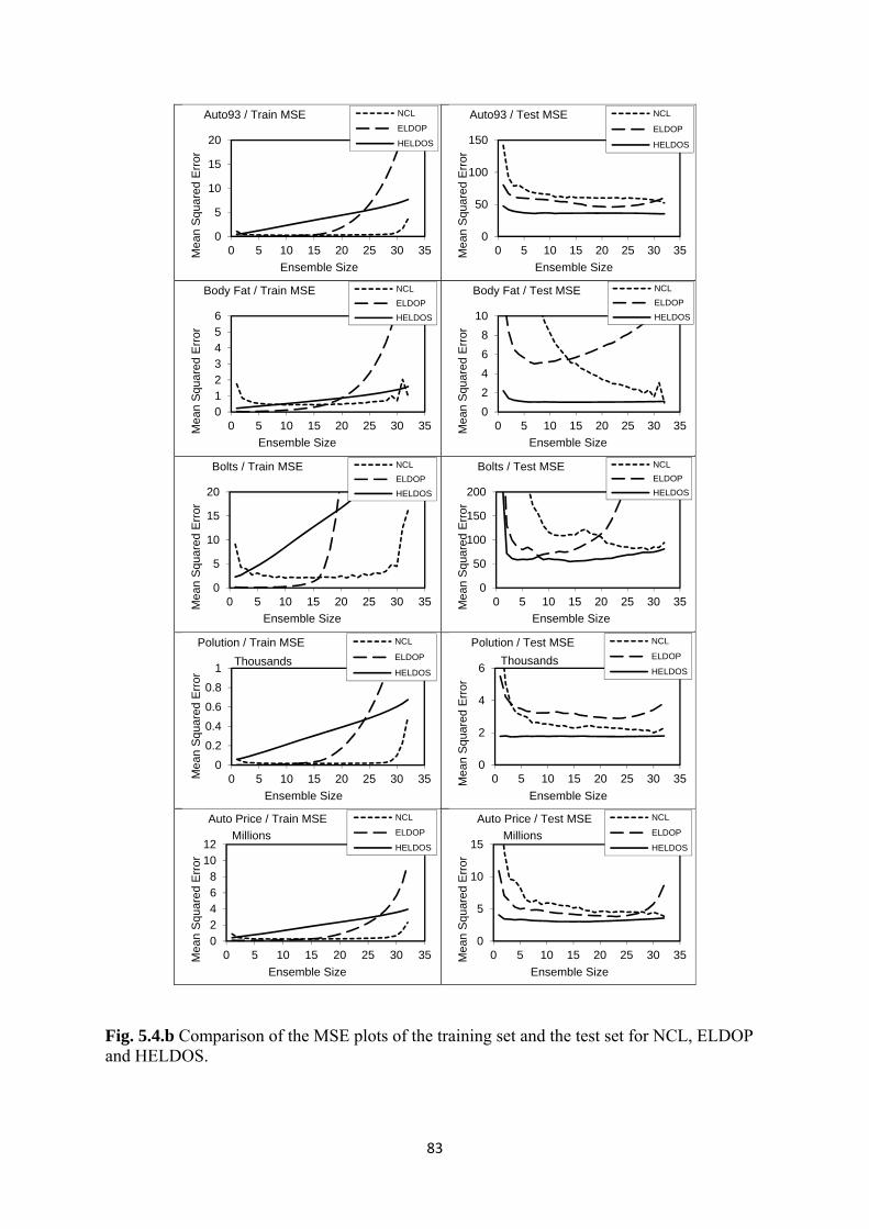
83  

 

Fig. 5.4.b Comparison of the MSE plots of the training set and the test set for NCL, ELDOP and HELDOS.

0

5

10

15

20

0 5 10 15 20 25 30 35Mea

n S

quar

ed E

rror

Ensemble Size

Auto93 / Train MSE NCL

ELDOP

HELDOS

0

50

100

150

0 5 10 15 20 25 30 35Mea

n S

quar

ed E

rror

Ensemble Size

Auto93 / Test MSE NCL

ELDOP

HELDOS

0123456

0 5 10 15 20 25 30 35Mea

n S

quar

ed E

rror

Ensemble Size

Body Fat / Train MSE NCL

ELDOP

HELDOS

0

2

4

6

8

10

0 5 10 15 20 25 30 35Mea

n S

quar

ed E

rror

Ensemble Size

Body Fat / Test MSE NCL

ELDOP

HELDOS

0

5

10

15

20

0 5 10 15 20 25 30 35Mea

n S

quar

ed E

rror

Ensemble Size

Bolts / Train MSE NCL

ELDOP

HELDOS

0

50

100

150

200

0 5 10 15 20 25 30 35Mea

n S

quar

ed E

rror

Ensemble Size

Bolts / Test MSE NCL

ELDOP

HELDOS

0

0.2

0.4

0.6

0.8

1

0 5 10 15 20 25 30 35Mea

n S

quar

ed E

rror

Thousands

Ensemble Size

Polution / Train MSE NCL

ELDOP

HELDOS

0

2

4

6

0 5 10 15 20 25 30 35Mea

n S

quar

ed E

rror

Thousands

Ensemble Size

Polution / Test MSE NCL

ELDOP

HELDOS

02468

1012

0 5 10 15 20 25 30 35Mea

n S

quar

ed E

rror

Millions

Ensemble Size

Auto Price / Train MSE NCL

ELDOP

HELDOS

0

5

10

15

0 5 10 15 20 25 30 35Mea

n S

quar

ed E

rror

Millions

Ensemble Size

Auto Price / Test MSE NCL

ELDOP

HELDOS

84  

5.5 Conclusion

Continuing from chapter 4 the dynamic pruning approach has been further investigated in this

chapter. The research undertaken here has been to incorporate pruning into the learning

process, but pruning is done through ordering the predictors according to their performance

and selecting from this order. By doing so, diversity is encouraged in the predictors that are

trained. Here again the distributed approach taken, based on the individual patterns in the

training set, in the ensemble selection has helped to reduce the ensemble error in the

regression problem.

In this chapter two novel dynamic methods are introduced for regression, one which

combines ensemble learning with dynamic pruning and the other that combines learning

approaches. Experimental results show that test error has been reduced in both methods by

introducing pruning in the training phase of ensembles as well as combining two learning

methods. The motivation for the proposed methods is based on the introduction of diversity

through varied learning methods [61].

In DESIP [119] the ensemble selection for a test pattern is based on the closest

training instance and therefore a search is necessary to determine the pruned ensemble, while

in ELDOP the ensemble is trained with the pruned selection, therefore eliminating the need to

search. In NCL, OA, DESIP and HELDOS the entire ensemble is utilized in training, while

ELDOP trains only the selected members of the ensemble, with a commensurate reduction in

training time. For the data sets used in this experiment, HELDOS or ELDOP achieves best

results, but which of the two methods performs best is data dependent.

As further work, varying the percentage of split for the ensemble member selection

would help to understand the variation of ensemble accuracy by means of varying predictor

diversity. An extension to this investigation would be to have multiple splits in the ensemble

85  

of predictors and training them with different methods. Also as future work varying the value

of K in K-means clustering would help to understand the partitioning of the predictor outputs

based on diversity. Using the Bias/Variance decomposition in the theoretical formulation of

the processes in ELDOP and HELDOS would help to show why the error is low compared to

the other methods.

In chapter 6, the methods described in chapters 3,4 and 5 are applied to a signal

calibration problem. 

 

   

86  

Chapter6

Signal Calibration using Ensemble Systems

A novel method of using a learning paradigm for the calibration of nonlinear

systems is proposed in this chapter. With this it addresses the non-existent use of

learning systems to provide corrective measures in calibration. In this method

the learned system provides corrections directly to the nonlinear device to

linearize the system output without the need for an additional calculation to

produce the corrections. In many calibration tasks a model of the nonlinear

system is created and with its help corrections are calculated to linearize the

system output. The proposed method makes these two steps transparent by

learning the corrective step instead. Therefore the learned system is able to

directly linearize the nonlinear system output. The ensemble methods described

in chapters 3,4 and 5 have been used in the above approach in signal calibration

in an attempt to increase the calibration accuracy .

6.1 Introduction

In signal generation applications, calibration of the signal source is essential for the proper

operation of the device. Bounded by the nonlinearities of the components such as amplifiers

and attenuators within the signal generator, the output signal can only be maintained at the

desired level if these nonlinearities are known and compensated for.  A feedback system

sensing the output would enable this compensation to be performed dynamically at runtime.

But without runtime feedback, prior knowledge of the output behaviour is required in order to

perform output error correction. Usually by modelling the nonlinear characteristics, it is

possible to calculate the corrective effects to maintain a known relationship between the

87  

desired and the actual. The corrections, also known as calibration, are generated by seeking

the model’s output that corresponds to the actual behaviour of the non-linear system. In most

situations of a model being generated for calibration, a learning system such as a neural

network can be utilised. However, there has been no attempt to use a learned system to

generate the actual corrections directly. By this it is meant that the corrective action, rather

than the non-linear behaviour, is learned by the neural network which can then be used

directly to drive the nonlinear system. The proposed method is novel wherein a learning

system is used to learn the corrective function for the signal calibration of a nonlinear system.

This method is described in section 6.2.1.

Neural networks have been used for this application due to their ability to learn an

underlying function from given samples. The function in this application is the corrective

action required to linearize the output. The trained neural network can be then used to predict

output values, which is consistent with the function learnt. An ensemble of these neural

networks further makes the output impervious to noise in the training data with its

generalising ability. An ensemble of neural networks also improves the prediction accuracy

by the diversity each network acquires during training. However some predictors can be

detrimental to the collective ensemble output due to the variation with which it has learnt the

underlying function in the training data. These predictors will only perform well in some

parts of the function and therefore would have to be pruned out of the ensemble.

By taking into consideration both training and pruning aspects of ensemble neural

network predictors, the ensemble methods proposed in chapters 3,4 and 5 in this thesis have

been implemented in the signal calibration application for improving the prediction accuracy,

and with it the calibration accuracy. In contrast to the static ensemble method’s approach to

pruning and combining of predictors, where the pruned ensemble is fixed in its usage phase,

88  

the dynamic approach can utilise all the predictors to the ensemble’s advantage by selecting

the predictors based on their performance spatially in the distribution of the learnt function.

In Dynamic Ensemble Selection and Instantaneous Pruning (DESIP) described in chapter 4,

the training set is used to determine the predictor order that shows the best performance for

every pattern in the training set. Recursive Feature Elimination (RFE) described in chapter 3,

has been used as a method of ordering. Therefore a different predictor selection is realised for

every training pattern. This allows all the predictors to be utilised and the selection of the

predictor order to be distributed spatially across the training set. DESIP performs better, by

having a training set that fully covers the underlying function, that is learnt by the ensemble

of predictors, with the least space between the training patterns. This also helps in the test

phase when the closest training pattern to the test pattern is searched, where the predictor

order of this test pattern can produce the best possible prediction.

In Ensemble Learning and Dynamic Ordered Pruning (ELDOP) and Hybrid Ensemble

Learning and Dynamic Ordered Selection (HELDOS) described in chapter 5, diversity is

introduced by both methods to the predictors while training as part of the learning process. To

enhance diversity the pruning or selection of predictors, and the training of predictors are

performed in succession for every pattern in the training set. By ordering the predictors based

on their performance on a training pattern, the first method trains only the most diverse

predictors, while the second method splits the ensemble into two sub ensembles, of which

one contains the most diverse members and other less diverse. The most diverse members are

then trained using Negative Correlation Learning (NCL) method while the less diverse

members are trained independently. During the test phase of these methods a subset of the

trained predictors are chosen differently depending on their performance on the test sample.

Therefore the ensemble selection is dynamic during predicting the output, which improves

the prediction accuracy.

89  

6.2 Signal Calibration

Calibration can be automated by learning device characterisation in machines with the help of

Neural Networks. In [124] neural networks have been used to establish the relationship

between inputs and outputs, between geometric parameters in [125], between functional

models in [126]. In [127] the neural network has learnt the functional difference between an

actual test bed and its abstract model that has enabled fast simulation of a problem while

maintaining accuracy. A look-up table containing calibration data for the calculation of

parameters for a correction filter has been implemented in [128]. Here the calibration data

consists of performance data of the signal generator to which the correction filters are

applied. As described in [129] and in the methods used in many of the calibration

applications a model of the nonlinear device has been created for determining the correction

that is applied to the primary input signal of the nonlinear system. This is shown in figure 6.1

where the Input Signal is used by the Nonlinear System Model to generate the modifications

needed to correct the Input Signal to linearize the Nonlinear System.

Fig. 6.1. Calibration with signal correction using model of nonlinear system.

An efficient way of providing the corrected Input signals to the Nonlinear System is to learn

the corrective action in order to directly apply the correct signals to the Nonlinear System,

bypassing the need to perform corrections on the Input Signal. In this approach an ensemble

Nonlinear System Input Signal 

System Output

Nonlinear System Model 

Corrected Input Signal 

Correction

90  

of Neural Networks learns the corrective action and function as a Learned Model of

Corrective Action to provide Correct Input Signals to the Nonlinear System. This is shown

in figure 6.2 where the Correct Input Signal from the Model is interrogated using the Input

Signal and applied directly to the Nonlinear System. Apart from the efficiency and speed

gains, an advantage of this approach is the robustness to noise, where a noisy Input Signal

would be filtered by the generalisation ability of the ensemble of Neural Network predictors.

Fig. 6.2. Calibration with correct signal provided by a model that has learnt the corrective action.

6.2.1 Learning the Calibration Function

The proposed signal calibration method using a learned system has been applied to a portable

Radar Threat Simulator (RTS) device to demonstrate its operation. Here a Radio Frequency

(RF) attenuator is used to adjust the output of the RTS to simulate weak signal levels

associated with far-off emitters in a radar environment. Any nonlinear behaviour exhibited by

the system is corrected through calibration. This is shown in figure 6.3 where the RF Source

block generates the RF signal within the RTS and the Attenuator Function block applies

correct attenuation on the power level of this signal to achieve the desired output attenuation

of the radar signal. The correct attenuation is provided by interrogating the Learned Model

for the Correct Control Signals that is applied to the nonlinear Attenuator Function.

Nonlinear System Input Signal 

System OutputLearned Model of Corrective 

Action 

Correct InputSignal 

91  

Fig. 6.3. Block diagram of RTS with Learned Model providing Correct Control Signals.

The Learned Model of Corrective Action is an ensemble of Neural Network predictors that

has learned the corrective action required by the nonlinear attenuator. Here the process of

learning requires samples of the attenuator that exhibit the nonlinear behaviour. These

samples then form the training set for training the Neural Network predictors using the

backpropagation update rule. In the RTS application, each training sample consists of three

features, namely the Frequency of the radar signal, the Attenuation Demand and the Output

Attenuation. In order to train the ensemble of Neural Network predictors to learn the

corrective action for the attenuator, the Frequency and the Output Attenuation are selected as

input features to the Neural Networks while the Attenuation Demand is selected as the

target. This is shown in the top diagram in figure 6.4. This arrangement ensures that the

trained Neural Network predictors output the Correct Control Signals that can drive the

attenuator directly when interrogated with the Frequency and the Attenuation Demand as

input features, enabling linear operation of the Attenuator Function. With this training

regime, the Neural Network has learnt the corrective action needed to provide the Correct

Control Signals for the Attenuator Function to operate linearly.

Attenuator Function 

RF In

Attenuation Demand 

Learned Model of Corrective Action  (Ensemble of Neural Network) 

Frequency 

Correct Control Signals

Output  Attenuation RF Source 

RF Out

92  

Fig. 6.4. Training and Interrogation of Neural Networks for the Learned Model.

Therefore when interrogating the Neural Network predictors the Frequency and the

Attenuation Demand are used as inputs to the Neural Networks while the output of the

ensemble of Neural Networks is the Correct Control Signals for the attenuator. This is

shown in the bottom diagram in figure 6.4. The system shown in figure 6.3 can also be

implemented with a calibration look-up table in place of the trained ensemble of Neural

Network predictors, where the control values in this table are populated by the Neural

Network predictors.

Here the prediction accuracy is important in order to meet tight specification

requirements of the RTS, since a large error in the predicted control value would produce

undesirable behaviour by the device, rendering the device unsuitable for its intended use.

Therefore in the real world this learning based application would be required to operate with

its own tight specification requirements. The resulting linearization of the attenuator

function is shown in in figure 6.5. The vertical variation in the Output Attenuation for the

User Demanded Attenuation shown in figure 6.5(a) is due to the nonlinearity of the

Frequency 

Output 

Attenuation 

Attenuation 

Demand 

Training 

Frequency Correct Control 

Signals Attenuation 

Demand 

Interrogation

Neural Network

Neural Network

93  

Attenuator Function. The linearized output shown in figure 6.5(b) is the calibrated output

using the Learned Model of Corrective Action.

(a)  (b) 

Fig. 6.5. Non-linear characteristics and the calibrated characteristics of the Radio Frequency Source Device.

6.2.2 Training Methods for the Learned Model

In order to improve the prediction accuracy in the Learned Model, the ensemble predictors

were trained using the methods described in chapters 3, 4 and 5. The methods described

suited the application since the input-output values of the application are continuous.

Recursive Feature Elimination (RFE) described in chapters 3 and 4 has been used to order

the ensemble members based on the feature ranking and eliminating method using internal

layer weights of the neural networks. This method, being a static method for determining the

order of the members, sets the pruning order of the ensemble for the Learned Model. This

method is compared with the ensemble member ordering using Ordered Aggregation (OA)

described in chapter 4. Dynamic Ensemble Selection and Instantaneous Pruning (DESIP)

also described in chapter 4 uses Reduced Error Pruning without Back Fitting for ordering

and selecting the ensemble members for the entire training set on a pattern by pattern basis.

This selection is then archived for retrieval during test. By using K-Nearest Neighbours

method the closest training pattern to the test pattern is selected and the order of the

01020304050607080

0 20 40 60 80

Out

put

Atte

nuat

ion

dB

User Demanded Attenuation dB

Non-linear Characteristics

0

10

20

30

40

50

60

70

0 20 40 60 80

Out

put

Atte

nuat

ion

dB

User Demanded Attenuation dB

Calibrated Characteristics

94  

ensemble members is thus determined dynamically for predicting the test output. In chapter

6, two training regimes for dynamically pruning the ensemble have been described [130]

[131]. In both these methods weight updating during training is performed on a pattern by

pattern basis. With this diversity is introduced while simultaneously training, as part of the

same learning process. In the first method, Ensemble Learning with Dynamic Ordered

Pruning (ELDOP), the ensemble is ordered for each training pattern based on the

performance of the ensemble on the training pattern and only the most diverse members are

trained. Therefore it is assumed that each ensemble member trains on different parts of the

dataset. In the second method, Hybrid Ensemble Learning with Dynamic Ordered Selection

(HELDOS), for each training pattern the ensemble is ordered and split into two sub-

ensembles based on their performance on the training pattern. The sub-ensemble with lower

combined error is trained using Negative Correlation Learning while the second sub-

ensemble is trained independently. The performance of each of these methods is compared

in section 6.3 and the performance improvements observed are highlighted.

6.3 Results

For this application, based on initial experiments, a neural network with 10 hidden layer

nodes was used as the predictor and the ensemble size is 100 predictors. The data set

consisted of 660 training instances and 630 test instances. Here ensemble methods OA, RFE,

DESIP, NCL, ELDOP and HELDOP have been applied to compare the performance

differences. In the initial comparison, static pruning method OA is compared with RFE and

DESIP. This is shown in table 6.1. In comparison to RFE, OA shows lower performance

than RFE and in figure 6.6 it can also be observed that a lower error is achieved by OA. In

comparison to the static methods OA and RFE, the dynamic method DESIP has performed

better giving the lowest error, which is shown in table 6.1 and figure 6.6.

95  

 

Fig. 6.6. Calibration application MSE performance of OA, RFE and DESIP using RE.

Table 6.1. Average MSE with Standard Deviation for 10 iterations, OA, RFE and DESIP/RE.

OA RFE DESIP/RE 0.2±0.07 0.21±0.05 0.13±0.03

The comparison of NCL, OA, DESIP with ELDOP and HELDOS is shown in table 6.2. The

results indicate that the dynamic methods ELDOP and HELDOS have outperformed the other

methods. The variation of the error with ensemble order is shown in figure 6.7.

 

Fig. 6.7. Calibration application MSE performance of NCL, OA, DESIP, ELDOP and HELDOS.

Table 6.2. Average MSE with Standard Deviation for 10 iterations, NCL, OA, DESIP, ELDOP and HELDOS.

NCL OA DESIP ELDOP HELDOS 0.14±0.06 0.20±0.07 0.13±0.03 0.09±0.05 0.07±0.03

Significant improvement is shown by ELDOP and HELDOS when compared to NCL.

Considering that NCL, ELDOP and HELDOS train the predictors on a pattern by pattern

basis, the performance improvement can be attributed to the dynamic selection of predictors

0.1

0.15

0.2

0.25

0.3

0 50 100Mea

n S

quar

ed E

rror

Subensemble Size

RF Source Device / Test MSEOA

RFE

DESIP

00.05

0.10.15

0.20.25

0.30.35

0.4

0 50 100

Mea

n S

quar

d E

rror

Ensemble Size

RF Source Device / Test MSE OADESIPELDOPHELDOSNCL

96  

in the training regime in both ELDOP and HELDOS. In ELDOP, after ordering the predictors

based on the performance on the training pattern, only the predictors that are diverse get

trained with the training pattern, leading to an ensemble of predictors that train on different

parts of the dataset. In HELOS, the hybrid method of NCL and independent training has

helped to improve the performance.

6.4 Conclusion

The calibration application described in this chapter learns the corrective action required to

provide correct signals to linearize the system output. By learning the corrective action rather

than modelling the nonlinear system, it has removed the need for applying the adjustments to

correct the input signal. An ensemble of neural network predictors has been utilized for

implementing the Learned Model. By selecting input features and the target in the training

data for training in the manner described in section 6.2.1 the neural network predictors are

automatically set to provide the correct input signals for the nonlinear system to linearize its

output. An added benefit in using neural network predictors for the Learned Model is its

resilience to noise. In a calibration system where a model is used to represent the nonlinear

behavior of the system, a noisy input would cause an erroneous correction to be made on the

input signal.

The performance of the ensemble of predictors has been improved with the dynamic

methods DESIP, ELDOP and HELDOS compared to OA, RFE and NCL. Since the

prediction accuracy of the ensemble is important in the entire input range of the calibration

application, the hybrid approach in HELDOS has been able to generalize for input values that

were not present in the training data.

   

97  

Chapter7

Conclusion and Future Work

Many applications in machine learning, such as text mining, anomaly detection, biomedical

informatics and device calibration use learning systems that work with large data bases. In

many of these data bases, original data may contain large number of features, running into

hundreds and thousands, and can lead to degradation in predictor performance. Among these

high dimensional data are the irrelevant and redundant features that should be removed to

reduce the complexity and ensure good generalisation performance. Ensemble predictors also

improve accuracy and stability of predictors, such as neural networks. The state-of-the-art

suggests that pruning ensembles has helped further improve accuracy and generalisation by

seeking sub-ensembles with diverse members. It is further emphasised that pruning

ensembles dynamically enhance the accuracy and the generalisation.

7.1 Conclusion

In the experiments using RFE with linear SVC weights, it has been observed that the

performance is sensitive to C, but in contrast, MLP ensembles were relatively insensitive to

the nodes and epochs. However, by searching over different kernels and values for C, a

comparable result to MLP ensemble performance is likely. In a bootstrapped MLP ensemble,

using RFE and the weights product for feature ranking is an effective way of eliminating

irrelevant features. It also has the added advantage of using the OOB estimate to tune

parameters and to determine when to stop eliminating features.

98  

Extending RFE approach to ensemble selection, a method is proposed in this thesis

for ensemble pruning by ranking the ensemble members using a trained combiner and its

weights product. Experimental results of this method suggest that the ranking criterion does

not highlight the diversity among the ensemble members, therefore shows poor performance.

The feature ranking approaches have been applied to a two-class problem in facial

action unit classification. Here the multi-class problem of detecting action units has been

decomposed into two-class problems using PCA and Error Correcting Output Coding

(ECOC) approaches. Experimental results show that optimised two-class classifiers give

slightly lower mean error rates than ECOC.

Dynamic ensemble pruning is an active area of research for both classification and

regression. In dynamic pruning a distributed approach is utilised by looking into the regional

diversity of the members in the problem space, thereby improving accuracy and

generalisation of the ensemble based on this regional diversity. Taking account of this,

DESIP has been proposed in chapter 4 as a novel method of dynamic pruning of ensemble

members. DESIP uses the training samples to establish the regional diversity of the members

and provides the mechanism by which to choose the appropriate pruned sub-ensemble based

on the distance from the test pattern to a training pattern. Experimental results show that test

error has been reduced by modifying the pruning based on an ordered ensemble using

Reduced Error Pruning without Back Fitting and choosing the closest training pattern based

on K-nearest neighbours, with K = 1, and L1 norm as distance measure. The performance

comparison between Euclidean distance and Mahalanobis distance shows comparable results.

In DESIP ensemble members are trained from bootstrapped training samples and the

training is epoch based, where after initialising the weights with random values the weight

99  

adjustments are made using the average error of an entire epoch of training samples.

Therefore a predictor is trained in the same manner on the same set of training samples. In

ELDOP and HELDOS it is aimed to selectively train on patterns of the training set. To do

this pruning has been incorporated into the learning process. Here pruning is performed

through ordering the predictors according to their performance and selecting from this order,

and in doing so, diversity is encouraged in the predictors. ELDOP and HELDOS, proposed in

chapter 5 are two novel dynamic methods, the former in which ensemble learning is

combined with dynamic pruning and the latter combines learning approaches. Experimental

results shows that test error has reduced in both methods by introducing pruning in the

training phase of ensembles as well as combining two learning methods. Compared with

DESIP, a search for the closest training pattern isn’t necessary to determine the pruned

ensemble in ELDOP, since the ensemble is trained with the pruned selection, therefore

eliminating the need to search. In both methods K-means clustering enables similar predictor

outputs to cluster together, which is aimed at separating the diverse groups of predictors.

The calibration application described in chapter 6 uses a learning mechanism that

learns the corrective action to provide corrections to a nonlinear device to linearize its output.

By learning the corrective action, rather than modelling the nonlinear system, it has removed

the need to apply corrections to the input of the nonlinear system. In this application neural

networks have been utilised for the learning task. The novel method proposed uses the neural

networks learning system to learn the corrective action by manipulating the input and output

features in the training data. The neural network thus trained provides correct inputs for the

nonlinear device to linearize its output. A benefit in using a learning system for this

application is its ability to populate a lookup-table containing the correct inputs to the

nonlinear device. Also with neural networks, the system is resilient to noise. Compared to a

model being used for seeking corrections to be applied to the input signal of the nonlinear

100  

device, the proposed method is efficient, where the neural network output is applied directly

to the nonlinear device. A significant improvement of this method of using a learning system

is the overall speed gain in the implementation of the calibration system. In a production

environment a calibration system implemented using a conventional lookup table requires all

entries in the table to be measured and placed in memory, while a learning system requires

relatively lesser number of measurements to train and the complete table is implemented by

interpolating between training points.

Since the calibration application is for a military grade device, the accuracy of the

prediction of the system is important to its operation and has to meet tight design

specifications. In order to obtain accurate input signals for the nonlinear system an ensemble

of neural networks has been utilised in this application and the proposed methods in chapters

3,4 and 5 have been implemented for performance comparison. Comparing DESIP, ELDOP

and HELDOS with OA, RFE and NCL, experimental results show that using dynamic

methods have improved the performance compared to static methods. A further performance

improvement is seen using ELDOP and HELDOS when compared to DESIP.

7.2 Limitations

The use of SVC ensembles suggests that ensemble classifiers with low bias achieve

better performance. However it isn’t possible to be definitive without searching over all

kernel and generalisation constants C.

The performance of DESIP can be low for small sample sized problems due to large

distances attributed to the limited number of training samples covering the problem space.

Thereby, with the distance between a test pattern and the chosen training pattern also being

large can render the selected ordering non-optimal for the test pattern. However the low

101  

performance shown on some datasets in the experimental results for DESIP may not be

attributed to this issue of small sample size and therefore would be an investigation for future

work.

7.3 Future Work

ECOC can detect combinations of aus and further work is aimed at determining

whether problem-dependent, rather than random ECOC codes can give better results.

Values greater than one would show the effects and variation of performance based

on K in the K-nearest neighbours method in DESIP. By increasing K, the regional sub-space

for ensemble pruning is increased. With this, one extreme for K is when it equals the entire

training space where the performance is based on the average order of the ensemble for all

test patterns. Therefore K being very large would be detrimental to the performance of the

ensemble. Along with varying the value of K, different distance measures would have to be

investigated. The effect of selecting relevant features in the dataset for the distance measure

is also an area of interest for future work.

The percentage split for the ensemble member selection in ELDOP and HELDOS can

be varied to investigate its effect on the ensemble accuracy. This would help to understand

the variation of ensemble accuracy by means of varying predictor diversity. An extension to

this investigation would be to have multiple splits in the ensemble of predictors and train

them with different ensemble learning methods. Also varying the value of K in K-means

clustering would help to understand the partitioning of the predictor outputs based on

diversity.

102  

As has been shown by Brown et al. [61], ambiguity decomposition and the bias-

variance-covariance decompositions in regression provide a quantification of diversity for

linearly weighted ensembles by linking it to the objective error criterion of mean squared

error. It is suggested in [61] that error correlation derived from the ambiguity decomposition

has influenced the design of ensemble learners, and also it has shown why ensemble

members that are diverse should be averaged for improved performance. Using these

approaches, as future work the processes in DESIP, ELDOP and HELDOS should be

investigated theoretically to understand the effects of diversity and improve accuracy and

generalisation. This analysis would help to show why the performance on some datasets for

DESIP has not improved and also why the performance on some datasets are better for

ELDOP than for HELDOS.

In the calibration application, the combined investigation of the performance effects

by varying K in K-nearest neighbours and different distance measures in DESIP, as well as

varying the percentage split, using different ensemble learning methods and varying K in K-

means clustering in ELDOP and HELDOS would help to improve accuracy and

generalisation of the methods used in the application. Active learning is another area to

investigate, considering that the measurements from the application are expensive. Also

transfer learning can help speed up the calibration process by leveraging knowledge from

earlier manifestations of the learning task.

   

103  

 

Bibliography 

[1] T. Windeatt , “Ensemble MLP classifier design,” Computational Intelligence

Paradigms, vol. 137, pp. 133 - 147, 2008.

[2] G. Brown , “Ensemble Learning,” Encyclopedia of Machine Learning, C. Sammut

and G. Webb (Eds), Springer Press, pp. 312 - 320, 2010.

[3] L. Breiman , “Bagging predictors,” Machine Learning, vol. 24, no. 2, pp. 123 - 140,

1996.

[4] Y. Freund and R. Schapire , “Experiments with a new boosting algorithm,”

International Conference on Machine Learning, vol. 96, pp. 148 - 156, 1996.

[5] H. Hotelling, “Analysis of a complex of statistical variables into principal

components,” Journal of educational psychology, vol. 24, no. 6, pp. 417 - 441, 1933.

[6] A. Hyvärinen, J. Karhunen and E. Oja, “Independent component analysis,” John

Wiley & Sons, vol. 46, 2004.

[7] T. Ho, “The random subspace method for constructing decision forests,” IEEE

Transactions on Pattern Analysis and Machine Intelligence, vol. 20, no. 8, pp. 832 -

844, 1998.

[8] T. Dietterich and G. Bakiri, “Solving multiclass learning problems via error-

correcting output codes,” Journal of Artificial intelligence research, vol. 2, pp. 263 -

286, 1995.

[9] T. Windeatt, “Accuracy/diversity and ensemble MLP classifier design,” IEEE

Transactions on Neural Networks, vol. 17, no. 5, pp. 1194 - 1211, 2006.

104  

[10] R. Banfield, L. Hall, K. Bowyer and W. Kegelmeyer, “Ensemble diversity measures

and their application to thinning,” Information Fusion, vol. 6, no. 1, pp. 49 - 62, 2005.

[11] R. Caruana, A. Niculescu-Mizil, G. Crew and A. Ksikes, “Ensemble selection from

libraries of models,” Proceedings of the twenty-first international conference on

Machine learning, ACM Press, p. 18, 2004.

[12] G. Martınez-Munoz and A. Suárez, “Aggregation ordering in bagging,” Proceedings

of the IASTED International Conference on Artificial Intelligence and Applications,

pp. 258 - 263, 2004.

[13] Q. Dai, T. Zhang and N. Liu, “A new reverse reduce-error ensemble pruning

algorithm,” Applied Soft Computing, vol. 28, pp. 237 - 249, 2015.

[14] G. Giacinto and F. Roli, “Dynamic classifier selection based on multiple classifier

behaviour,” Pattern Recognition, vol. 34, no. 9, pp. 1879 - 1881, 2001.

[15] L. Li, B. Zou, Q. Hu, X. Wu and D. Yu, “Dynamic classifier ensemble using

classification confidence,” Neurocomputing, vol. 99, pp. 581 - 591, 2013.

[16] S. Soares and R. Araújo, “A dynamic and on-line ensemble regression for changing

environments,” Expert Systems with Applications, vol. 45, no. 2, pp. 2935 - 2948,

2015.

[17] J. Quinlan, “Decision trees and decision-making,” IEEE Transactions on Systems,

Man and Cybernetics, vol. 20, no. 2, pp. 339 - 346, 1990.

[18] H. Almuallim and T. Dietterich, “Learning with many irrelevant features,”

Proceedings of the ninth National conference on Artificial intelligence, AAAI Press,

vol. 2, pp. 547 - 552, 1991.

[19] K. Kira and L. Rendell, “A practical approach to feature selection,” Proceedings of

the ninth international workshop on Machine Learning, Derek Sleeman and Peter

105  

Edwards (Eds), Morgan Kaufmann, pp. 249 - 256, 1992.

[20] M. Hall, “Correlation-based feature selection for discrete and numeric class machine

learning,” Proceedings of 17th Intentional Conference on Machine Learning, Morgan

Kaufmann, San Meteo CA, pp. 359 - 366, 2000.

[21] G. John, R. Kohavi and K. Pfleger, “Irrelevant features and the subset selection

problem,” Proceedings of the Eleventh International Conference on Machine

Learning, pp. 121 - 129, 1994.

[22] R. Kohavi, “Feature subset selection as search with probabilistic estimates,” AAAI fall

symposium on relevance, vol. 224, pp. 122 - 126, 1994.

[23] H. Liu and R. Setiono, “A probabilistic approach to feature selection - a filter

solution,” Proceedings of the thirteenth International Conference on Machine

Learning, Morgan Kaufmann, vol. 96, pp. 319 - 327, 1996.

[24] M. Dash and H. Liu, “Hybrid search of feature subsets,” Proceedings of Pacific Rim

International Conference on Artificial Intelligence (PRICAI), Springer, pp. 238 - 249,

1998.

[25] M. Dash and H. Liu, “Feature selection for clustering,” Proceedings of the 4th

Pacific-Asia Conference on Knowledge Discovery and Data Mining, Current Issues

and New Applications, Springer, vol. 1805, pp. 110 - 121, 2000.

[26] J. Yang and V. Honavar, “Feature subset selection using a genetic algorithm,”

Feature extraction, construction and selection, Springer US, vol. 453, pp. 117 - 136,

1998.

[27] L. Yu and H. Liu, “Feature selection for high-dimensional data: A fast correlation-

based filter solution,” Proceedings of the 20th International Conference on Machine

Learning, pp. 856 - 863, 2003.

106  

[28] L. Yu and H. Liu, “Efficient feature selection via analysis of relevance and

redundancy,” The Journal of Machine Learning Research, vol. 5, pp. 1205 - 1224,

2004.

[29] M. Malarvili, M. Mesbah and B. Boashash, “HRV feature selection based on

discriminant and redundancy analysis for neonatal seizure detection,” IEEE 6th

International Conference on Information, Communications & Signal Processing, pp.

1 - 5, 2007.

[30] C. Deisy, B. Subbulakshmi, S. Baskar and N. Ramaraj, “Efficient dimensionality

reduction approaches for feature selection,” International Conference on

Computational Intelligence and Multimedia Applications, vol. 2, pp. 121 - 127, 2007.

[31] J. Biesiada and W. Duch, “Feature selection for high-dimensional data—a Pearson

redundancy based filter,” Computer Recognition Systems, Springer, vol. 45, pp. 242 -

249, 2007.

[32] J. Biesiada and W. Duch, “A Kolmogorov-Smirnov Correlation-Based Filter for

Microarray Data,” Neural Information Processing, Springer, vol. 4985, pp. 285 - 294,

2008.

[33] M. Munson and R. Caruana, “On feature selection, bias-variance, and bagging,”

Machine Learning and Knowledge Discovery in Databases: Part II, LNCS, Springer,

vol. 5782, pp. 144 - 159, 2009.

[34] I. Guyon, J. Weston, S. Barnhill and V. Vapnik, “Gene selection for cancer

classification using support vector machines,” Machine learning, vol. 46, no. (1-3),

pp. 389 - 422, 2002.

[35] Y. Peng, Z. Wu and J. Jiang, “A novel feature selection approach for biomedical data

classification,” Journal of Biomedical Informatics, vol. 43, no. 1, pp. 15 - 23, 2010.

107  

[36] H. Liu and L. Yu, “Toward integrating feature selection algorithms for classification

and clustering,” IEEE Transactions on Knowledge and Data Engineering, vol. 17, no.

4, pp. 491 - 502, 2005.

[37] P. Narendra and K. Fukunaga, “A branch and bound algorithm for feature subset

selection,” IEEE Transactions on Computers, vol. 26, no. 9, pp. 917 - 922, 1977.

[38] S. Stearns, “On selecting features for pattern classifiers,” Proceedings of the 3rd

International Joint Conference on Pattern Recognition, pp. 71 - 75, 1976.

[39] P. Pudil, J. Novovičová and J. Kittler, “Floating search methods in feature selection,”

Pattern recognition letters, vol. 15, no. 11, pp. 1119 - 1125, 1994.

[40] R. Meiri and J. Zahavi, “Using simulated annealing to optimize the feature selection

problem in marketing applications,” European Journal of Operational Research, vol.

171, no. 3, pp. 842 - 858, 2006.

[41] L. Hansen and P. Salamon, “Neural network ensembles,” IEEE Transactions on

Pattern Analysis & Machine Intelligence, vol. 12, no. 10, pp. 993 - 1001, 1990.

[42] R. Schapire, “The strength of weak learnability,” Machine learning, vol. 5, no. 2, pp.

197 - 227, 1990.

[43] L. Kuncheva, “Combining Pattern Classifiers,” Methods and Algorithms, Wiley, New

York, 2004.

[44] R. Polikar, “Ensemble based systems in decision making,” Circuits and Systems

Magazine, IEEE, vol. 6, no. 3, pp. 21 - 45, 2006.

[45] N. Oza and K. Tumer, “Input decimation ensembles: Decorrelation through

dimensionality reduction,” 2nd Int. Workshop on Multiple Classifier Systems,

Springer, vol. 2096, pp. 238 - 247, 2001.

[46] L. Breiman, “Random forests,” Machine learning, vol. 45, no. 1, pp. 5 - 32, 2001.

108  

[47] N. Oza and K. Tumer, “Classifier ensembles: Select real-world applications,”

Information Fusion, vol. 9, no. 1, pp. 4 - 20, 2008.

[48] J. Rodriguez, L. Kuncheva and C. Alonso, “Rotation Forest, A new classifier

ensemble method,” IEEE Transactions on Pattern Analysis and Machine Intelligence,

vol. 28, no. 10, pp. 1619 - 1630, 2006.

[49] J. Kittler, M. Hatef, R. Duin and J. Matas, “On combining classifiers,” IEEE

Transactions on Pattern Analysis and Machine Intelligence, vol. 20, no. 3, pp. 226 -

239, 1998.

[50] T. Dietterich, “Ensemble methods in machine learning,” Multiple classifier systems,

LNCS, Springer, vol. 1857, pp. 1 - 15, 2000.

[51] L. Kuncheva, “A theoretical study on six classifier fusion strategies,” IEEE

Transactions on Pattern Analysis and Machine Intelligence, vol. 24, no. 2, pp. 281 -

286, 2002.

[52] F. Roli, G. Giacinto and G. Vernazza, “Methods for designing multiple classifier

systems,” Multiple Classifier Systems, LNCS, Springer, vol. 2096, pp. 78 - 87, 2001.

[53] N. Rooney, D. Patterson, S. Anand and A. Tsymba, “Dynamic integration of

regression models,” Multiple Classifier Systems, LNCS, Springer, vol. 3181, pp. 164 -

173, 2004.

[54] I. Witten and E. Frank, “Data Mining: Practical machine learning tools and

techniques,” Morgan Kaufmann, 2005.

[55] M. Perrone and L. CoopeR, “When networks disagree: Ensemble methods for hybrid

neural networks,” Neural Networks for Speech and Image Processing, R.J. Mammone

(Ed.), Chapman-Hall, 1993.

[56] L. Kuncheva and C. Whitaker, “Measures of diversity in classifier ensembles and

109  

their relationship with the ensemble accuracy,” Machine learning, vol. 51, no. 2, pp.

181 - 207, 2003.

[57] G. Brown, “Diversity in neural networks ensembles,” PhD thesis, University of

Birmingham, 2004.

[58] A. Krogh and J. Vedelsby, “Neural network ensembles, cross validation, and active

learning,” Advances in neural information processing systems, vol. 7, pp. 231 - 238,

1995.

[59] N. Ueda and R. Nakano, “Generalization error of ensemble estimators,” Proceedings

of the IEEE Conference on Neural Networks, vol. 1, pp. 90 - 95, 1996.

[60] G. Brown, J. Wyatt and P. Tino, “Managing diversity in regression ensembles,”

Machine Learning Research, vol. 6, pp. 1621 - 1650, 2005.

[61] G. Brown, J. Wyatt, R. Harris and X. Yao, “Diversity creation methods: A survey and

categorization,” Information Fusion, vol. 6, no. 1, p. 5 – 20, 2005.

[62] Y. Raviv and N. Intrator, “Bootstrapping with noise, an effective regularization

technique,” Connection Science, vol. 8, no. 3-4, pp. 355 - 372, 1996.

[63] T. Cai and X. Wu, “Research on ensemble learning based on discretization methods,”

Proceedings of the 9th International Conference on Signal Processing, pp. 1528 -

1531, 2008.

[64] B. Rosen, “Ensemble learning using de-correlated neural networks,” Connection

Science, vol. 8, no. 3-4, pp. 373 - 384, 1996.

[65] M. Islam, X. Yao and K. Murase, “A constructive algorithm for training cooperative

neural network ensembles,” IEEE Transactions on Neural Networks, vol. 14, no. 4, p.

820 – 834, 2003.

[66] D. Opitz and J. Shavlik, “Generating accurate and diverse members of a neural

110  

network ensemble,” Advances in Neural Information Processing Systems, vol. 8, p.

535 – 541, 1996.

[67] Y. Liu and X. Yao, “Ensemble learning via negative correlation,” Neural Networks,

vol. 12, no. 10, p. 1399 – 1404, 1999.

[68] Y. Liu, X. Yao and T. Higuchi, “Evolutionary ensembles with negative correlation

learning,” IEEE Transactions on Evolutionary Computation, vol. 4, no. 4, p. 380 –

387, 2000.

[69] G. Tsoumakas, I. Partalas and I. Vlahavas, “A taxonomy and short review of

ensemble selection,” workshop on supervised and unsupervised ensemble methods

and their applications, ECAI, pp. 41 - 46, 2008.

[70] D. Margineantu and T. Dietterich, “Pruning adaptive boosting,” International

Conference on Machine Learning, p. 211 – 218, 1997.

[71] G. Martinez-Muoz, D. Hernández-Lobato and A. Suarez, “An Analysis of Ensemble

Pruning Techniques Based on Ordered Aggregation,” IEEE Transactions on Pattern

Analysis and Machine Intelligence, vol. 31, no. 2, p. 245 – 259, 2009.

[72] G. Martínez-Muñoz and A. Suárez, “Using boosting to prune bagging ensembles,”

Pattern Recognition Letters, vol. 28, no. 1, p. 156 – 165, 2007.

[73] T. Windeatt and C. Zor, “Ensemble Pruning using Spectral Coefficients,” IEEE

Transactions on Neural Networks and Learning Systems, vol. 24, no. 4, p. 673 – 678,

2013.

[74] V. Soto, G. Martínez-Muñoz, D. Hernández-Lobato and A. Suárez, “A double

pruning algorithm for classification ensembles,” Multiple Classifier Systems, LNCS,

Springer, vol. 5997, p. 104 – 113, 2010.

[75] D. Hernández-Lobato, G. Martinez-Muoz and A. Suarez, “Statistical instance-based

111  

pruning in ensembles of independent classifiers,” IEEE Transactions on Pattern

Analysis and Machine Intelligence, vol. 32, no. 2, p. 364 – 369, 2009.

[76] G. Giacinto, F. Roli and G. Fumera, “Design of effective multiple classifier systems

by clustering of classifiers,” Proceedings. 15th International Conference on Pattern

Recognition, vol. 2, p. 160 – 163, 2000.

[77] Y. Zhang, S. Burer and W. Street, “Ensemble pruning via semi-definite

programming,” Journal of Machine Learning Research, vol. 7, p. 1315 – 1338, 2006.

[78] C. Merz, “Dynamical selection of learning algorithms,” Artificial Intelligence and

Statistics, Fisher D., and Lenz H.J. (Eds), Learning from Data, LNS, Springer NY,

vol. 112, pp. 281 - 290, 1996.

[79] G. Giacinto and F. Roli, “Adaptive selection of image classifiers,” Proceedings of the

9th International Conference on Image Analysis and Processing, p. 38 – 45, 1997.

[80] A. Ko, R. Sabourin and A. Britto Jr, “From dynamic classifier selection to dynamic

ensemble selection,” Pattern Recognition, vol. 41, no. 5, p. 1718 – 1731, 2008.

[81] M. Skurichina and R. Duin, “Combining feature subsets in feature selection,”

Proceedings 6th International Workshop Multiple Classifier Systems, LNCS,

Springer, vol. 3541, p. 165 – 174, 2005.

[82] R. Kohavi and G. John, “Wrappers for feature subset selection,” Journal of Artificial

Intelligence, special issue on relevance, vol. 97, no. 1-2, p. 273 – 324, 1997.

[83] I. Guyon and A. Elisseeff, “An introduction to variable and feature selection,” The

Journal of Machine Learning Research, vol. 3, p. 1157 – 1182, 2003.

[84] Y. Tian, T. Kanade and J. Cohn, “Recognizing action units for facial expression

analysis,” IEEE Transactions on Pattern Analysis and Machine Intelligence, vol. 23,

no. 2, pp. 97 - 115, 2001.

112  

[85] G. Donato, M. Bartlett, J. Hager, P. Ekman and T. Sejnowski, “Classifying facial

actions,” IEEE Transactions on Pattern Analysis and Machine Intelligence, vol. 21,

no. 10, p. 974 – 989, 1999.

[86] T. Windeatt and K. Dias, “Feature ranking ensembles for facial action unit

classification,” IAPR Third International Workshop on Artificial Neural Networks in

Pattern Recognition, LNCS, Springer, vol. 5064, p. 267 – 279, 2008.

[87] T. Windeatt, M. Prior, N. Effron and N. Intrator, “Ensemble-based Feature Selection

Criteria,” Procedings of Conference on Machine Learning Data Mining, p. 168 – 182,

2007.

[88] R. Bryll, T. Gutierrez-Osuna and F. Quek, “Attribute bagging: improving accuracy of

classifier ensembles by using random feature subsets,” Pattern Recognition, vol. 36,

no. 6, p. 1291 – 1302, 2003.

[89] T. Windeatt and M. Prior, “Stopping criteria for ensemble-based feature selection,”

Multiple Classifier Systems, LNCS, Springer, vol. 4472, p. 271 – 281, 2007.

[90] T. Bylander, “Estimating generalization error on two-class datasets using out-of-bag

estimates,” Journal of Machine Learning, vol. 48, no. 1-3, p. 287 – 297, 2002.

[91] T. Windeatt and R. Ghaderi, “Coding and decoding strategies for multi-class learning

problems,” Information Fusion, vol. 4, no. 1, p. 11 – 21, 2003.

[92] Y. Freund and R. Schapire, “A decision-theoretic generalization of on-line learning

and an application to boosting,” Journal of computer and system sciences, vol. 55, no.

1, p. 119 – 139, 1997.

[93] G. James, “Variance and bias for general loss functions,” Journal of Machine

Learning, vol. 51, no. 2, p. 112 – 135, 2003.

[94] L. Breiman, “Arcing classifier,” The annals of statistics, vol. 26, no. 3, p. 801 – 849,

113  

1998.

[95] E. Kong and T. Dietterich, “Error-Correcting Output Coding Corrects Bias and

Variance,” Proceedings of 12th International Conference on Machine Learning, p.

313 – 321, 1995.

[96] C. Hsu, H. Huang and S. Dietrich, “The ANNIGMA-wrapper approach to fast feature

selection for neural nets,” IEEE Transactions on System, Man and Cybernetics-Part

B:Cybernetics, vol. 32, no. 2, p. 207 – 212, 2002.

[97] K. Fukunaga, “Introduction to statistical pattern recognition,” Academic Press, 1990.

[98] N. Efron and N. Intrator, “The effect of noisy bootstrapping on the robustness of

supervised classification of gene expression data,” Proceedings of 14th IEEE Signal

Processing Society Workshop Machine Learning for Signal Processing, p. 411 – 420,

2004.

[99] M. Bartlett, L. Littlewort, C. Lainscsek, I. Fasel and J. Movellan, “Machine learning

methods for fully automatic recognition of facial expressions and facial actions,”

IEEE International Conference on Systems, Man and Cybernetics, vol. 1, p. 592 –

597, 2004.

[100] P. Silapachote, D. Karuppiah and A. Hanson, “Feature selection using AdaBoost for

face expression recognition,” Proceedings of Conference on Visualization, Imaging

and Image Processing, p. 84 – 89, 2004.

[101] B. Fasel and J. Luettin, “Automatic facial expression analysis: a survey,” Pattern

Recognition, vol. 36, no. 1, p. 259 – 275, 2003.

[102] F. Van Der Heijden, R. Duin, D. De Ridder and D. Tax, “Classification, parameter

estimation and state estimation,” John Wiley & Sons, 1990.

[103] L. Pretchelt, “PROBEN1-A set of neural network benchmark problems and

114  

benchmarking rules,” Technical Report 21/94, University Karlsruhe, Germany, 1994.

[104] C. Merz and P. Murphy, “UCI Repository of Machine Learning Databases,”

http://www.ics.uci.edu/~mlearn/ML Repository.html, 1998.

[105] T. Kanade, J. Cohn and Y. Tian, “Comprehensive database for facial expression

analysis,” Proceedings of Fourth IEEE International Conference on Automatic Face

and Gesture Recognition, p. 46 – 53, 2000.

[106] T. Dietterich, “Approximate statistical tests for comparing supervised classification

learning algorithms,” Neural computation, vol. 10, no. 7, p. 1859 – 1923, 1998.

[107] G. Valentini and T. Dietterich, “Bias-variance analysis of support vector machines for

the development of SVM-based ensemble methods,” Journal of Machine Learning

Research, vol. 5, p. 725 – 775, 2004.

[108] G. Tsoumakas, I. Partalas and I. Vlahavas, “An ensemble pruning primer,”

Applications of supervised and unsupervised ensemble methods, Springer, pp. 1 - 13,

2009.

[109] D. Hernández-Lobato, G. Martínez-Muñoz and A. Suárez, “Empirical analysis and

evaluation of approximate techniques for pruning regression bagging ensembles,”

Neurocomputing, vol. 74, no. 12, p. 2250 – 2264, 2011.

[110] Z. Zhou, J. Wu and W. Tang, “Ensembling neural networks: many could be better

than all,” Artificial intelligence, vol. 137, no. 1, p. 239 – 263, 2002.

[111] E. Dos Santos, R. Sabourin and P. Maupin, “A dynamic overproduce-and-choose

strategy for the selection of classifier ensembles,” Pattern Recognition, vol. 41, no.

10, p. 2993 – 3009, 2008.

[112] P. Cavalin, R. Sabourin and C. Suen, “Dynamic selection of ensembles of classifiers

using contextual information,” Multiple Classifier Systems ,LNCS, Springer, vol.

115  

5997, p. 145 – 154, 2010.

[113] Z. Shen and F. Kong, “Dynamically weighted ensemble neural networks for

regression problems,” Machine Learning and Cybernetics, vol. 6, p. 3492 – 349,

2004.

[114] T. Windeatt and K. Dias, “Ensemble approaches to facial action unit classification,”

Proceedings of the 13th Iberoamerican congress on Pattern Recognition, CIARP,

LNCS, Springer, vol. 5197, pp. 551 - 559, 2008.

[115] H. Dubey and V. Pudi, “CLUEKR: CLUstering Based Efficient kNN Regression,”

Advances in Knowledge Discovery and Data Mining, LNCS, Springer, vol. 7818, p.

450 – 458, 2013.

[116] UCI-Machine-Learning-Repository, “Regression Datasets,”

https://archive.ics.uci.edu/ml/datasets.html?format=&task=reg&att=&area=&numA

tt=&numIns=&type=&sort=nameUp&view=table.

[117] WEKA-Machine-Learning-Repository, “Datasets,”

http://www.cs.waikato.ac.nz/ml/weka/datasets.html.

[118] R. Nanculef, C. Valle, H. Allende and C. Moraga, “Ensemble learning with local

diversity,” International Conference in Artificial Neural Networks, LNCS, Springer,

vol. 4131, pp. 264 - 273, 2006.

[119] K. Dias and T. Windeatt, “Dynamic Ensemble Selection and Instantaneous Pruning

for Regression,” European Symposium on Artificial Neural Networks, ESANN, p. 64

3– 648 , 2014.

[120] K. Dias and T. Windeatt, “Dynamic Ensemble Selection and Instantaneous Pruning

for Regression Used in Signal Calibration,” Artificial Neural Networks and Machine

Learning, ICANN, Springer, vol. 8681, pp. 475 - 482, 2014.

116  

[121] G. Brown and X. Yao, “On the effectiveness of negative correlation learning,”

Proceedings on First UK Workshop on Computational Intelligence, pp. 57 - 62, 2001.

[122] J. MacQueen, “Some methods for classification and analysis of multivariate

observations,” Proceedings of the fifth Berkeley symposium on mathematical statistics

and probability, vol. 1, no. 14, pp. 281 - 297, 1967.

[123] L. Kuncheva, “Clustering-and-selection model for classifier combination,”

Proceedings of Fourth International Conference on Knowledge-Based Intelligent

Engineering Systems and Allied Technologies, vol. 1, p. 185 – 188, 2000.

[124] S. Khan, D. Shahani and A. Agarwala, “Sensor calibration and compensation using

artificial neural network,” ISA transactions, vol. 42, no. 3, pp. 337 - 352, 2003.

[125] M. Mendonça, I. Da Silva and J. Castanho, “Camera calibration using neural

networks,” Journal of WSCG, vol. 10, no. 1-3, pp. POS61 - POS68, 2002.

[126] D. Wang, X. Liu and X. Xu, “Calibration of the arc-welding robot by neural

network,” IEEE Proceedings of International Conference on Machine Learning and

Cybernetics, vol. 7, pp. 4064 - 4069, 2005.

[127] E. Liu, L. Cuthbert, J. Schormans and G. Stoneley, “Neural network in fast simulation

modelling,” Proceedings of the IEEE-INNS-ENNS International Joint Conference on

Neural Networks, vol. 6, pp. 109 - 113, 2000.

[128] J. Earls and Tektronix Inc., “Apparatus for generation of corrected vector wideband

RF signals”. Patent International Patent, EP Register - EP2541811 A2, 2013.

[129] A. Fernandez, “System and Method of Digital Linearization in Electronic Devices”.

Patent US Patent, US20090058521 A1, 2009.

[130] K. Dias and T. Windeatt, “Ensemble Learning with Dynamic Ordered Pruning for

Regression,” European Symposium on Artificial Neural Networks, pp. 125 - 130,

117  

2015.

[131] K. Dias and T. Windeatt, “Hybrid Dynamic Learning Systems for Regression,”

Advances in Computational Intelligence, LNCS, Springer, vol. 9095, pp. 464 - 476,

2015.