Embed Size (px)
Citation preview

Dynamic analysis of concrete gravity dam-reservoir systems by Wavenumber
approach for the general reservoir base condition
Mehran Jafari1*, Vahid Lotfi2
Department of Civil and Environmental Engineering,
Amirkabir University of Technology, Tehran, Iran
Abstract
Different approaches are utilized for dynamic analysis of concrete gravity dam-
reservoir systems. The rigorous approach for solving this problem employs a two-
dimensional semi-infinite fluid element (i.e., hyper-element). Recently, a technique was
proposed for dynamic analysis of dam-reservoir systems in the context of pure finite element
programming which was referred to as the Wavenumber approach. Of course, certain
limitations were imposed on the reservoir base condition in the initial form of this technique
to simplify the problem. However, this is presently discussed for the general reservoir base
condition, contrary to the previous study which was merely limited to the full reflective
reservoir base case. In this technique, the wavenumber condition is imposed on the truncation
boundary or the upstream face of the near-field water domain. The method is initially
described. Subsequently, the response of an idealized triangular dam-reservoir system is
obtained by this approach, and the results are compared against the exact response. Based on
this investigation, it is concluded that this approach can be envisaged as a great substitute for
the rigorous type of analysis under the general reservoir base condition.
Keywords: frequency domain analysis, concrete gravity dams, Wavenumber approach,
reservoir bottom absorption, truncation boundary
1. Introduction
Dynamic analysis of concrete gravity dam-reservoir systems can be carried out rigorously by
FE-(FE-HE) method in the frequency domain. This means that the dam is discretized by
plane solid finite elements, while, the reservoir is divided into two parts, a near-field region
(usually an irregular shape) in the vicinity of the dam and a far-field part (assuming uniform
1 M.Sc., Corresponding author, Email: [email protected]
Department of Civil and Environmental Engineering,
Amirkabir University of Technology, Tehran, Iran.
Tel.: (+98) 9128077954 2 Professor, Email: [email protected]
Department of Civil and Environmental Engineering,
Amirkabir University of Technology, Tehran, Iran.

depth) which extends to infinity in the upstream direction. The former region is discretized by
plane fluid finite elements and the latter part is modeled by a two-dimensional fluid hyper-
element ([1], [2], [3]). It is well-known that employing fluid hyper-elements would lead to
the exact solution of the problem. However, it is formulated in the frequency domain and its
application in this field has led to many special purpose programs which were demanding
from programming point of view.
On the other hand, engineers have often tried to solve this problem in the context of pure
finite element programming (FE-FE method of analysis). In this approach, an often simplified
condition is imposed on the truncation boundary or the upstream face of the near-field water
domain. Thus, the fluid hyper-element is actually excluded from the model. Some of these
widely used simplified conditions ([4], [5]), may result in significant errors if the reservoir
length is small, and it might lead to high computational cost if the truncation boundary is
located at far distances. The main advantage of these conditions is that it can be readily used
for time domain analysis. Thus, they are vastly employed in nonlinear seismic analysis of
concrete dams.
Of course, there have also been many studies in the last three decades to develop more
accurate absorbing boundary conditions to be applied for similar fluid-structure or soil-
structure interaction problems. Perfectly matched layer ([6], [7], [8], [9], [10], [11]) and, high-
order non-reflecting boundary condition ([12], [13], [14], [15], [16], [17], [18]) are among the
two main popular groups of methods which researchers have applied in their attempts. It is
emphasized that these techniques have become very popular in recent years due to the fact
that they could be applied in time domain as well as the frequency domain. However, it
should be realized that they are not very attractive in the frequency domain. This is well
understood, having in mind that they are not very simple to be used and more importantly,
they are compared with the hyper-element alternative which produces exact results no matter
how small the reservoir near-field length is considered.
In the present study, the FE-FE analysis technique is employed as the basis of a proposed
method for dynamic analysis of concrete dam-reservoir system in the frequency domain,
which is referred to as the Wavenumber approach. The method is simply applying an
absorbing boundary condition on the truncation boundary which is referred to as the
Wavenumber condition. It is as simple as employing Sommerfeld or Sharan condition on the
truncation boundary. It should be mentioned that this is an extension and generalization of a
previous study which was merely limited to the full reflective reservoir base case ([19], [20]).
This is presently discussed for the general reservoir base condition.
In the following sections of the article, the method of analysis is initially explained.
Subsequently, the response of an idealized triangular dam is studied due to horizontal ground
motion for several alternatives employed as absorbing boundary condition. In each case, as
well as the proposed option, the results are compared against the exact solution. The results
are provided for the moderate as well as low reservoir lengths. Moreover, both full reflective
and absorptive reservoir base conditions are studied.

2. Method of analysis
As mentioned, the analysis technique utilized in this study is based on the FE-FE method,
which is applicable for a general concrete gravity dam-reservoir system. The coupled
equations can be obtained by considering each region separately and then combine the
resulting equations.
2.1 Dam Body
Concentrating on the structural part, the dynamic behavior of the dam is described by the
well-known equation of structural dynamics ([21]):
T
g Mr Cr K r M Ja B P (1)
where Μ , C and K in this relation represent the mass, damping and stiffness matrices of
the dam body. Moreover, r is the vector of nodal relative displacements, J is a matrix with
each two rows equal to a 2×2 identity matrix (its columns correspond to a unit horizontal and
vertical rigid body motion), and ga denotes the vector of ground accelerations. Furthermore,
B is a matrix which relates vectors of hydrodynamic pressures (i.e., P ), and its equivalent
nodal forces.
Let us now consider harmonic excitation with frequency ω, and limit the present study to the
horizontal ground motion only. It is well known that the response will also behave harmonic
(i.e., i( ) ( ) er rtt ). Thus, Eq. (1) can be expressed as:
2 h T
g(1 2 i) = M K r MJa B P (2)
In this relation, it is assumed that the damping matrix of the dam is of hysteretic type. This
means:
(2 / )C K (3)
Moreover, it should be emphasized that the superscript h on the acceleration vector refers to
the horizontal type of excitation. That is:
x
h g
g
a
0
a (4)
2.2 Water Domain
Assuming water to be linearly compressible and neglecting its viscosity, its small irrotational
motion (Fig. 1) is governed by the wave equation ([22], [23]):
2 2
2 2 2
10 in and
p pp D
x y c
(5)
where p is the hydrodynamic pressure and, c is the pressure wave velocity in water. The
boundary conditions for reservoir surface and bottom are as follows:

on the water sur, ce0 fap (6a)
g , at the reservoir s bottomnpa q p
n
(6b)
Herein, is the water density and n denotes the outward (with respect to fluid region)
perpendicular direction at the reservoir bottom. Moreover, the admittance or damping
coefficient q utilized in the above equation, may be related to a more meaningful wave
reflection coefficient ([24]):
1
1
q c
q c (7)
which is defined as the ratio of the amplitude of the reflected hydrodynamic pressure wave to
the amplitude of a vertically propagating pressure wave incident on the reservoir bottom. For
a full reflective reservoir bottom condition, is equal to 1 which leads to 0q .
One can apply the weighted residual approach to obtain the finite element equation of the
fluid domain, which may be written as:
e e e e e G P H P R (8)
With the following definitions:
T
2
1d
G N N
e
e
c (9a)
T T1d
H N N N N
e
e
x x y y
(9b)
1( )d
R N
e
e e
n p
(9c)
With N being the vector of element’s shape functions, and ,N Nx y denote its partial
derivatives with respect to x, y, respectively. It is also worthwhile to emphasize that the
superscript ( e ) states that these matrices are related to the element level. The directional
derivative n p in relation (9c), can take three forms on different boundaries of the reservoir
(Fig. 1):
On the upstream boundary of the reservoir ( I ): One can apply different absorbing
boundary conditions which will be discussed in next section.
At the bottom of the reservoir ( II ), one can utilize Eq. (6b) as mentioned previously:
g
n
n p a q p (10a)
On the dam-reservoir interface ( III ):

n np u (10b)
where nu is the total acceleration of fluid particles normal to the dam-reservoir interface. It is
also noted that there must be compatibility of acceleration between the fluid and solid
particles in that direction.
In general, an element may have all three above-mentioned boundary condition types. Thus,
one can write eR vector as follows:
I II III
e ee e R R RR (11)
Of course, it is possible that some of these boundary condition types are not applied for a
certain element, which that part should be eliminated for that specific element. It is easily
shown that one would obtain the following relations by utilizing (10a) and (10b) in (9c),
respectively:
III
h
I g II B J aR L Pe e e e eq (12a)
IIII
h
II g( ) B r J aRe ee e
(12b)
With the following definitions:
i
T
i s d ; i II , III
B Nn Ne
T ee (13a)
IIII
T1d
e
ee
L N N (13b)
Herein, n represents a unit outward normal vector. Moreover, sN is the matrix of adjacent
solid element shape functions utilized to interpolate accelerations in horizontal and vertical
directions. It is worthwhile to mention that from practical point of view, the value of non-zero
solid and fluid shape functions are essentially equal on the common fluid-solid interface.
Substituting (12a) and (12b) into (11) will result in:
h
I II g R L P B r BR J ae e e e e e ee q (14)
With the following definition:
II III
e e e B B B (15)
It should also be noted that the relative acceleration at boundary II is identically equal to
zero. Subsequently, (14) can be substituted in (8) which yields:
h
II I g( ) G P L P H P R B r B J ae e e e e e e e e e eq t (16)
The equivalent form of this equation in the frequency domain would be:
2 2 h
II I gi ( ) G P L P H P R B r B J ae e e e e e e e e e eq (17)

Here, II
eL is a matrix, which corresponds to the absorption of energy at reservoir’s bed. By
assembling the element equations and imposing the free surface condition (6a), one would
obtain the overall FE equation of the fluid domain:
2 2 h
II I gi G P L P H P R Br BJaq (18)
In this equation, IR is obtained by assembling the boundary integrals of Eq. (9c) on I .
2.3 Dam-reservoir system
The necessary equations for both dam and reservoir domains were developed in the previous
sections. Thus, combining the main relations (18) and (2) would result in the FE equations of
the coupled dam-reservoir system in its initial form for the frequency domain:
h2 Tg
h2 2g III
(1 2 i)
)(i )(
M J arM K B
B J a RPB G L Hq
(19)
It is noted from the above equation that the vector IR still needs to be defined by some
appropriate condition. This is related to the truncated boundary I which will be discussed
below.
2.4 Modification due to truncation boundary contribution
The effect of truncation boundary will be treated in this section. For this purpose, let us now
assume that this boundary (i.e., I ) is vertical (i.e. along y-direction) and consider a harmonic
plane wave with unit amplitude and frequency propagating along a direction which makes
an angle with negative x-direction. This may be written in many different forms such as:
i( ) k x y tp e (20a)
(i ) (cos ) (sin ) c x y c t
p e
(20b)
With the following relations being valid:
cos kc
(21a)
sinc
(21b)
22 2
2 k
c
(21c)
It is easily verified that the following condition is appropriate for the truncated boundary
based on the assumed traveling wave (i.e, Eq. (20a)):
i 0
pk p
x (22)
Employing (22) in (9c), it yields:

II (i ) L PRee ek (23)
with the following definition:
II
T1d
L N N
e
ee
(24)
Assembling IRe for all fluid elements adjacent to truncation boundary leads to:
II (i )R L Pk (25)
This can now be substituted in (19) to obtain the FE equations of the coupled dam-reservoir
system in its final form for the frequency domain:
h2 Tg
2 h2 2gI II
(1 2 i)
( )i i( )
M J arM K B
B J aPB G L L Hk q
(26)
It is also noticed that the lower matrix equation of (26) is multiplied by 2 in this process to
obtain a symmetric dynamic stiffness matrix for the dam-reservoir system.
2.5 Theoretical background pertinent to parameter k
The major remaining concept is the determination of parameter k . The relevant theoretical
background will be discussed in this section. Of course, there are different available options
which will be actually presented in the next section. However, before a discussion on that, it
is worthwhile to review some salient aspects on the exact analytical solution available for the
domain D (Fig. 1) which is extremely helpful in this regard. It is reminded that this domain is
actually eliminated from our problem.
This is a regular semi-infinite region with constant depth H extending to infinity in the
upstream direction. The base of this region may be absorptive (i.e, 1 ) or fully reflective
(i.e, 1 or 0q ). As mentioned, this was limited merely to the latter case in a previous
study ([19]). However, the more general case will be treated herein (i.e, no restriction on ).
Of course, it should be emphasized that we are still considering merely horizontal ground
excitation similar to that study. Under these circumstances, the exact solution for this region
may be written as follows ([23]):
i( )
1
i( , , ) cos( ) sin( )
jk x t
j j jjj
qp x y t B y y e (27)
It is noted that the solution is composed of different modes, and amplitude jB depends on the
existing conditions on the downstream face of that region. While, parameters j are calculated
through the following Eigenvalue problem:
icos( H) sin( H) 0
j j
j
q (28)
Herein, H represents the water depth. Moreover, parameters j and jk are related as:
22 2
2 j jk
c
(29)
By employing (29), one would obtain:
22
2i j jk
c
(30)
Although, there are two options in this definition, the negative sign is merely admissible for a
semi-infinite region extending to infinity in the negative x-direction as in our present case.
This is due to the fact that we are only interested in the modes which are decaying and
propagating towards the upstream direction.
2.5.1 Full reflective reservoir base condition (i.e., special case)
Let us now concentrate on the special case of full reflective base condition (i.e, 1 or 0q
). Under these circumstances, relations (27) and (28) are simplified as follows:
i( )
1
( , , ) cos( )
jk x tj j
j
p x y t B y e (31)
cos( H) 0 j (32)
Moreover, the eigenvalues j are readily obtained:
(2 1)
2 H
j
j (33)
It is also noted that the j-th wavenumber ( jk ) becomes zero at a cut-off frequency referred to
as the j-th natural frequency of the reservoir (i.e., rj ). This is obtained by substituting (33)
in (30) under that condition which results in:
(2 1)
2 H
r
j
j c (34)
Eq. (30) with the admissible negative sign, may also be written as:
2
2
i (2 1)1
(2 1)
j
jk
c j
(35)
with the help of dimensionless frequency :
1
r
(36)

2.6 Different options for defining parameter k
Let us now describe some of the available options for selecting parameter k in Eq. (26):
Alternative 1.
The first option could be that one presumes the assumed planar wave is impinging the
truncation boundary perpendicularly. Thus, the angle is zero, and k is readily found from
(21a):
kc
(37)
It is worthwhile to mention that, this may also be envisaged as the limiting case for each jk
(Eq. 35) as goes to infinity. Substituting (37) into (22) leads to what is known as
Sommerfeld boundary condition for the frequency and time domains, respectively ([4]):
i
pp
x c
(38a)
1
p p
x c t (38b)
Alternative 2.
The second option is to define k based on an approximation of the first wavenumber
assuming the full reflective base condition as a simplification. Thus, let us consider the first
wavenumber for that special case (i.e., substitute 1j in (35)):
21
i1
k
c
(39)
By employing the estimate√1 − Ω2 ≈ (1 + iΩ) on (39) and utilizing (34), (36), it yields:
i2 H
kc
(40)
Substituting (40) into (22) leads to what is known as Sharan boundary condition for the
frequency and time domains, respectively ([5]):
i
2 H
pp p
x c
(41a)
1
2 H
p pp
x c t
(41b)
Alternative 3.
The third option is what is proposed in this study. That is to define k based on different
wavenumbers for various frequency ranges. In particular, use the following strategy:
1 ; initially k k as a default value (42a)

2 22 2
12 2; if Real( ) 0 and Real( ) 0 for 2
j j jk k j
c c (42b)
In which jk is solved through equation (30) with a negative sign option. Of course, this
requires the computation of j which is solved through the Eigenvalue problem (28) by the
well-known Newton-Raphson approach.
It should be mentioned that for the special case of full reflective base condition, the strategy
may be equivalently written as follows:
1 2; 0 3 (0 )
rk k for or (43a)
1; (2 1) (2 1) ( ) 2
r rj j jk k for j j or and j (43b)
In which jk is solved through equation (35). This is what was proposed in the previous study
([19]). It is also worthwhile to mention that for the special case, k would be either a real
number or a pure imaginary number. While in the general case, it could be a complex number
having both real and imaginary components.
It was mentioned above that in general, the Eigenvalues j are solved through (28) by
utilizing the Newton-Raphson algorithm. This is carried out herein for the first five modes
and the results are depicted in Fig. 2, which is similar to the work of Fenves and Chopra
([24]).
3. Modeling and Basic Parameters
The introduced methodology is employed to analyze an idealized dam-reservoir system. The
details about modeling aspects such as discretization, basic parameters and the assumptions
adopted are summarized in this section.
3.1 Models
An idealized triangular dam with vertical upstream face and a downstream slope of 1:0.8 is
considered on a rigid base. The dam is discretized by 20 isoparametric 8-node plane-solid
finite elements.
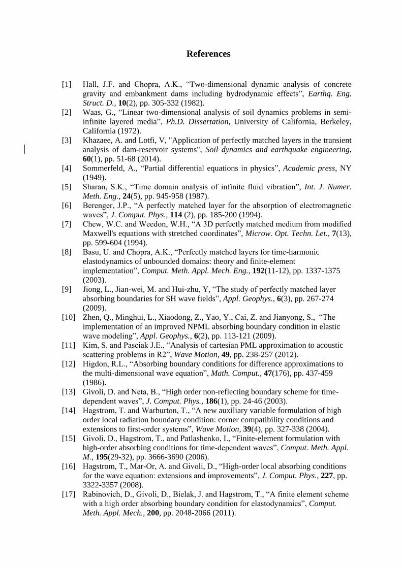
As for the water domain, two strategies are adopted (Fig. 3). For the FE-FE method of
analysis which is our main procedure, only the reservoir near-field is discretized and the
absorbing boundary condition is employed on the upstream truncation boundary according to
different alternatives discussed. The length of this near-field region is denoted by L and water
depth is referred to as H. Three cases are considered. These are in particular the L/H values of
0.2, 1 and 4 which represent low, moderate and high reservoir lengths. This region is
discretized by 5, 25 and 100 isoparametric 8-node plane-fluid finite elements for the three
above-mentioned L/H values, respectively.
For the FE-(FE-HE) method of analysis, the reservoir domain is divided into two regions.
The near-field region is discretized by fluid finite elements, and the far-field is treated by a
fluid hyper-element. Of course, it should be emphasized that this option is merely utilized to
obtain the exact solution ([25]). Moreover, it is well-known that the results are not sensitive
in this case to the length of the reservoir near-field region or L/H value.

3.2 Basic Parameters
The dam body is assumed to be homogeneous and isotropic with linearly viscoelastic
properties for mass concrete:
Elastic modulus ( )dE a27.5 GP
Poison's ratio 0.2
Unit weight 324.8 kN/m
Hysteretic damping factor ( )d 0.05
The impounded water is taken as inviscid and compressible fluid with unit weight equal to 39.81 kN/m , and pressure wave velocity 1440 m/sec.c
4. Results
It should be emphasized that all results presented herein, are obtained by the FE-FE method
discussed, under different absorbing conditions applied on the truncation boundary. The only
exception is for what is referred to as the exact response. That special case is carried out by
the FE-(FE-HE) analysis technique.
The initial part of the study relates to a dam-reservoir system with a moderate near-field
reservoir length (i.e., L/H=1(Fig. 3a)). This is examined for two different assumptions of full
reflective and absorptive reservoir base conditions (i.e., =1 and 0.75 ). For each model,
three cases are considered. The only difference between these cases, are the type of absorbing
boundary condition imposed on the truncation boundary. These are in particular based on
alternatives I, II and III (i.e, Sommerfeld, Sharan, and Wavenumber condition, respectively).
The transfer function for the horizontal acceleration at dam crest with respect to horizontal
ground acceleration, are presented in Fig. 4 for these three cases with the full reflective
reservoir base assumption ( =1 ). It is noted that response in each case is plotted versus the
dimensionless frequency. The normalization of excitation frequency is carried out with
respect to 1 , which is defined as the natural frequency of the dam with an empty reservoir on
rigid foundation. Moreover, it is noticed that all cases are compared with the exact response.
It is observed that the response for Sommerfeld condition case has significant error near the
fundamental frequency of the system where the first major peak occurs. For the second case
(Sharan B.C.), the error reduces at the first major peak (compared to the first case); however,
it is observed that the response maintains a similar pattern. Moreover, error increases at the
second major peak for this case, which shows the deficiency of Sharan condition with respect
to Sommerfeld B.C. for that frequency range.
The third case is related to the Wavenumber approach. It is observed that the response agrees
very well with the exact response and this initial result for this technique reveals the
promising behavior of this alternative.
Subsequently, similar plots are illustrated in Fig. 5 for the same three alternatives with the
absorptive reservoir base assumption ( = 0.75 ).
It is observed that both Sommerfeld and Sharan cases still have noticeable errors near the
fundamental frequency of the system, although, it is reduced in comparison with the full
reflective cases mentioned above. For the Wavenumber approach, the response is predicted
very well and the agreement with exact result is almost perfect for this case.
In the second part of this study, it was decided to investigate the behavior of three alternatives
I, II and III (i.e, Sommerfeld, Sharan, and Wavenumber approaches) for low near-field
reservoir lengths. For this purpose, a very low reservoir length (i.e., L/H=0.2 (Fig. 3b)) is
considered that is a challenging test for examining any type of absorbing boundary condition.
Similar to the moderate reservoir length, this is examined for two different assumptions of
full reflective and absorptive reservoir base conditions (i.e., =1 and 0.75 ).
The responses for the full reflective reservoir base condition ( =1 ) are presented in Fig. 6. It
is observed that there are significant errors in the responses for the Sommerfeld and Sharan
condition cases. Moreover, the errors have increased in comparison with the moderate
reservoir length results (Fig 6 versus Fig. 4). For the Wavenumber approach, the response is
still close to the exact response in most frequency ranges. However, there exist errors in the
range of 5% at the major peaks of the response. This is still believed to be a remarkable result
for such a challenging test.
Similar plots are illustrated in Fig. 7 for the same three alternatives with the absorptive
reservoir base assumption ( = 0.75 ). It is observed that there are still significant errors for
the Sommerfeld and Sharan condition cases. However, as expected, the errors have decreased
with respect to the full reflective reservoir condition (Fig 7 versus Fig. 6). For the
Wavenumber approach, it is observed that the error at the first major peak of the response
now diminishes with respect to the full reflective reservoir base condition (Fig 7 versus Fig.
6), and the response agrees relatively well with the exact response for the whole frequency
range.
In the last part of this study, it seemed worthwhile to investigate the behavior of three
alternatives I, II and III (i.e, Sommerfeld, Sharan, and Wavenumber approaches) for high
near-field reservoir lengths. For this purpose, a relatively high reservoir length (i.e., L/H=4 )
is considered. Similar to the previous reservoir lengths, this is examined for two different
assumptions of full reflective and absorptive reservoir base conditions (i.e., =1 and 0.75 ).
The responses for the full reflective reservoir base condition ( =1 ) are presented in Fig. 8. It
is noticed that responses for sommerfeld and Sharan condition cases improves greatly in
comparison with the low or even moderate length results discussed previously (Fig. 8 versus
Fig. 6 or 4). However, some kinds of noise or distortion are noticed in the response of both
these cases especially for higher frequencies. As for the Wavenumber approach, it is noticed
that the response agrees very well with the exact response, similar to the behavior noticed for
the moderate reservoir length. Moreover, there are slight signs of distortions in the response
for the high reservoir length, contrary to what was noticed for the other two well-known
alternatives I and II (Sommerfeld and Sharan condition cases).
Similar plots are also illustrated in Fig. 9 for the same three alternatives with the absorptive
reservoir base assumption ( = 0.75 ). It is observed that all three alternatives reveal good
behavior and very close agreements are obtained with respect to exact response for the whole
frequency range under these circumstances (i.e., high reservoir length and absorptive
reservoir base assumption ( = 0.75 )).
Overall, it could be concluded that the maximum error for the Wavenumber approach is in
the range of 5% at the major peaks of the response. This occurs only for the very low
reservoir lengths and full reflective reservoir base condition. This is a remarkable result for
any kind of robust truncation boundary simulation that one may expect. It is also worthwhile
to mention that in general, the fundamental frequency of the system is not captured correctly
when both Sommerfeld and Sharan B.C. are employed unless the reservoir length is selected
as a high value. This is especially true for cases in which low reservoir lengths are utilized in
the model (Figs. 6 and 7). However, the fundamental frequency of the system is captured
correctly for the Wavenumber approach, even in cases of low reservoir length (Figs. 6c and
7c).

5. Conclusions
The formulation based on FE-FE procedure for dynamic analysis of concrete dam-reservoir
systems, was reviewed. Moreover, several options were discussed for imposing a local type
of absorbing condition on the truncation boundary of the water domain. A special purpose
finite element program was enhanced for this investigation. Thereafter, the response of an
idealized triangular dam was studied due to horizontal ground motion for different
alternatives employed as absorbing boundary condition. The main approach which was
emphasized and proposed in this study is referred to as the Wavenumber approach.
Overall, the main conclusions obtained by the present study can be listed as follows:
In regard to Sommerfeld and Sharan absorbing condition:
In general, the fundamental frequency of the system is not captured correctly for both
of these approaches unless the reservoir length is selected as a high value. This is
especially true for cases in which low reservoir lengths are utilized in the model.
There are significant errors occurring on the response at the fundamental frequency of
the system for low or even moderate reservoir lengths. The error decreases for the
absorptive reservoir base condition or as the reservoir length increases.
Obviously, the main advantage of these two conditions is that both of them can be
readily utilized in time domain, as well as frequency domain.
In regard to Wavenumber absorbing condition:
The fundamental frequency of the system is captured correctly for the Wavenumber
approach, even in cases of low reservoir length.
It is concluded that the maximum error for the Wavenumber approach is in the range
of 5% at the major peaks of the response. This occurs only for the very low reservoir
lengths and full reflective reservoir base condition. This is a remarkable result for any
kind of robust truncation boundary simulation that one may expect.
Obviously, the main disadvantage of this condition is that it cannot be utilized in time
domain, and it is only suitable for frequency domain.
The Wavenumber approach is ideal from programming point of view due to the local
nature of Wavenumber condition imposed on truncation boundary. It can also be
deemed as a great substitute for the rigorous FE-(FE-HE) type of analysis which is
heavily relying on a hyper-element as its main core. It is undeniable that the rigorous
approach is significantly more complicated from programming point of view and also
much more computationally expensive.
References
[1] Hall, J.F. and Chopra, A.K., “Two-dimensional dynamic analysis of concrete
gravity and embankment dams including hydrodynamic effects”, Earthq. Eng.
Struct. D., 10(2), pp. 305-332 (1982).
[2] Waas, G., “Linear two-dimensional analysis of soil dynamics problems in semi-
infinite layered media”, Ph.D. Dissertation, University of California, Berkeley,
California (1972).
[3] Khazaee, A. and Lotfi, V, "Application of perfectly matched layers in the transient
analysis of dam-reservoir systems", Soil dynamics and earthquake engineering,
60(1), pp. 51-68 (2014).
[4] Sommerfeld, A., “Partial differential equations in physics”, Academic press, NY
(1949).
[5] Sharan, S.K., “Time domain analysis of infinite fluid vibration”, Int. J. Numer.
Meth. Eng., 24(5), pp. 945-958 (1987).
[6] Berenger, J.P., “A perfectly matched layer for the absorption of electromagnetic
waves”, J. Comput. Phys., 114 (2), pp. 185-200 (1994).
[7] Chew, W.C. and Weedon, W.H., “A 3D perfectly matched medium from modified
Maxwell's equations with stretched coordinates”, Microw. Opt. Techn. Let., 7(13),
pp. 599-604 (1994).
[8] Basu, U. and Chopra, A.K., “Perfectly matched layers for time-harmonic
elastodynamics of unbounded domains: theory and finite-element
implementation”, Comput. Meth. Appl. Mech. Eng., 192(11-12), pp. 1337-1375
(2003).
[9] Jiong, L., Jian-wei, M. and Hui-zhu, Y, “The study of perfectly matched layer
absorbing boundaries for SH wave fields”, Appl. Geophys., 6(3), pp. 267-274
(2009).
[10] Zhen, Q., Minghui, L., Xiaodong, Z., Yao, Y., Cai, Z. and Jianyong, S., “The
implementation of an improved NPML absorbing boundary condition in elastic
wave modeling”, Appl. Geophys., 6(2), pp. 113-121 (2009).
[11] Kim, S. and Pasciak J.E., “Analysis of cartesian PML approximation to acoustic
scattering problems in R2”, Wave Motion, 49, pp. 238-257 (2012).
[12] Higdon, R.L., “Absorbing boundary conditions for difference approximations to
the multi-dimensional wave equation”, Math. Comput., 47(176), pp. 437-459
(1986).
[13] Givoli, D. and Neta, B., “High order non-reflecting boundary scheme for time-
dependent waves”, J. Comput. Phys., 186(1), pp. 24-46 (2003).
[14] Hagstrom, T. and Warburton, T., “A new auxiliary variable formulation of high
order local radiation boundary condition: corner compatibility conditions and
extensions to first-order systems”, Wave Motion, 39(4), pp. 327-338 (2004).
[15] Givoli, D., Hagstrom, T., and Patlashenko, I., “Finite-element formulation with
high-order absorbing conditions for time-dependent waves”, Comput. Meth. Appl.
M., 195(29-32), pp. 3666-3690 (2006).
[16] Hagstrom, T., Mar-Or, A. and Givoli, D., “High-order local absorbing conditions
for the wave equation: extensions and improvements”, J. Comput. Phys., 227, pp.
3322-3357 (2008).
[17] Rabinovich, D., Givoli, D., Bielak, J. and Hagstrom, T., “A finite element scheme
with a high order absorbing boundary condition for elastodynamics”, Comput.
Meth. Appl. Mech., 200, pp. 2048-2066 (2011).

[18] Samii, A. and Lotfi, V., “High-order adjustable boundary condition for absorbing
evanescent modes of waveguides and its application in coupled fluid-structure
analysis”, Wave Motion, 49(2), pp. 238-257 (2012).
[19] Lotfi, V. and Samii, A., “Dynamic analysis of concrete gravity dam-reservoir
systems by Wavenuber approach in the frequency domain”, Earthquakes and
Structures, 3(3-4), pp. 533-548 (2012).
[20] Lotfi, V. and Samii, A., “Frequency Domain Analysis of Concrete Gravity Dam-
Reservoir Systems by Wavenumber Approach” , Proc. 15th World Conference on
Earthquake Engineering, Lisbon, Portugal (2012a).
[21] Zienkiewicz, O.C., Taylor, R.L. and Zhu, J.Z., “The Finite Element Method”,
Butterworth-Heinemann (2013).
[22] Chopra, A.K., “Hydrodynamic pressure on dams during earthquake”, J. Eng.
Mech.-ASCE, 93, pp. 205-223 (1967).
[23] Chopra, A.K., Chakrabarti, P. and Gupta, S., “Earthquake response of concrete
gravity dams including hydrodynamic and foundation interaction effects”, Report
No. EERC-80/01, University of California, Berkeley (1980).
[24] Fenves, G. and Chopra, A.K., “Effects of reservoir bottom absorption and dam-
water-foundation interaction on frequency response functions for concrete gravity
dams”, Earthq. Eng. Struct. D., 13, pp. 13-31 (1985).
[25] Lotfi, V., “Frequency domain analysis of gravity dams including hydrodynamic
effects”, Dam Engineering, 12(1), pp. 33-53 (2001).
Mehran Jafari, received his M.S. degree in civil engineering from the Amirkabir University of Technology (Tehran Polytechnic), Tehran, Iran in 2014, where he also received his B.S. degree in 2011 respectively. His research interests include: Fluid-Structure Interaction, Finite Element, Structural Analysis.
Vahid Lotfi, was born on 1960 in Tehran, Iran. He received his BS, MS and PhD in civil
engineering from the University of Texas at Austin, USA. He joined Amirkabir University of
Technology, Tehran, in 1986, and has been full professor at that university since 2005. His
research interests include: Finite Element, Fluid-Structure Interaction, Concrete Dams and
Earthquake Engineering.

Figures Captions
Fig. 1: Schematic view of a typical dam-reservoir system. The near-field reservoir domain 𝛺,
the truncation boundary Γ1 and the far-field region D (excluded in the FE-FE type of analysis.
Fig. 2: Variation of λ𝑗with excitation frequency for the general case of reservoir base
condition.
Fig. 3: The dam-reservoir discretization for; (a) FE-FE Model (L/H=1), (b) FE-FE Model
(L/H=0.2), (c) FE-(FE-HE) Model (L/H=1)
Fig. 4: Horizontal acceleration at dam crest due to horizontal ground motion for the moderate
reservoir length and full reflective reservoir base condition (𝐿/𝐻 = 1, 𝛼 = 1) under different
absorbing boundary condition alternatives; (a) Sommerfeld, (b) Sharan, (c) Wavenumber
Fig. 5: Horizontal acceleration at dam crest due to horizontal ground motion for the moderate
reservoir length and absorptive reservoir base condition (𝐿/𝐻 = 1, 𝛼 = 0.75) under different
absorbing boundary condition alternatives; (a) Sommerfeld, (b) Sharan, (c) Wavenumber
Fig. 6: Horizontal acceleration at dam crest due to horizontal ground motion for the low
reservoir length and full reflective reservoir base condition (𝐿/𝐻 = 0.2, 𝛼 = 1) under
different absorbing boundary condition alternatives; (a) Sommerfeld, (b) Sharan, (c)
Wavenumber
Fig. 7: Horizontal acceleration at dam crest due to horizontal ground motion for the low
reservoir length and absorptive reservoir base condition (𝐿/𝐻 = 0.2, 𝛼 = 0.75) under
different absorbing boundary condition alternatives; (a) Sommerfeld, (b) Sharan, (c)
Wavenumber
Fig. 8: Horizontal acceleration at dam crest due to horizontal ground motion for the high
reservoir length and full reflective reservoir base condition (𝐿/𝐻 = 4 , 𝛼 = 1) under different
absorbing boundary condition alternatives; (a) Sommerfeld, (b) Sharan, (c) Wavenumber
Fig. 9: Horizontal acceleration at dam crest due to horizontal ground motion for the high
reservoir length and full reflective reservoir base condition (𝐿/𝐻 = 4 , 𝛼 = 0.75) under
different absorbing boundary condition alternatives; (a) Sommerfeld, (b) Sharan, (c)
Wavenumber

Fig. 1
Fig. 2
Fig. 3

Fig. 4

Fig. 5

Fig. 6

Fig. 7

Fig. 8

Fig. 9


![Gravity Dam Design[1]](https://img.pdfslide.us/doc/110x75/545a2372b1af9f37608b5959/gravity-dam-design1.jpg)