Dynamic Algorithms for Graph Coloring

Sayan Bhattacharya∗ Deeparnab Chakrabarty† Monika Henzinger‡

Danupon Nanongkai§

Abstract

We design fast dynamic algorithms for proper vertex and edge colorings in a graph undergoing edgeinsertions and deletions. In the static setting, there are simple linear time algorithms for (∆ + 1)- vertexcoloring and (2∆ − 1)-edge coloring in a graph with maximum degree ∆. It is natural to ask if we canefficiently maintain such colorings in the dynamic setting as well. We get the following three results. (1)We present a randomized algorithm which maintains a (∆ + 1)-vertex coloring with O(log ∆) expectedamortized update time. (2) We present a deterministic algorithm which maintains a (1 + o(1))∆-vertexcoloring with O(polylog ∆) amortized update time. (3) We present a simple, deterministic algorithmwhich maintains a (2∆ − 1)-edge coloring with O(log ∆) worst-case update time. This improves therecent O(∆)-edge coloring algorithm with O(

√∆) worst-case update time [BM17BM17].

∗Corresponding author. University of Warwick, UK. Email: S.Bhattacharya@warwick.ac.uk†Dartmouth College, USA. Email: deeparnab.chakrabarty@dartmouth.edu‡University of Vienna, Austria. Email: monika.henzinger@univie.ac.at§KTH, Sweden. Email: danupon@gmail.com

i

Contents

1 Introduction 11

2 Our Techniques for Dynamic Vertex Coloring 332.1 An overview of our randomized algorithm. . . . . . . . . . . . . . . . . . . . . . . . . . . . 332.2 An overview of our deterministic algorithm. . . . . . . . . . . . . . . . . . . . . . . . . . . 55

3 A Randomized Dynamic Algorithm for ∆ + 1 Vertex Coloring 663.1 Preliminaries. . . . . . . . . . . . . . . . . . . . . . . . . . . . . . . . . . . . . . . . . . . 663.2 Maintaining the hierarchical partition. . . . . . . . . . . . . . . . . . . . . . . . . . . . . . 773.3 The recoloring subroutine. . . . . . . . . . . . . . . . . . . . . . . . . . . . . . . . . . . . 12123.4 The complete algorithm and analysis. . . . . . . . . . . . . . . . . . . . . . . . . . . . . . 1313

4 A Deterministic Dynamic Algorithm for (1 + o(1))∆ Vertex Coloring 14144.1 Notations and preliminaries. . . . . . . . . . . . . . . . . . . . . . . . . . . . . . . . . . . 14144.2 The algorithm. . . . . . . . . . . . . . . . . . . . . . . . . . . . . . . . . . . . . . . . . . . 17174.3 Bounding the amortized update time. . . . . . . . . . . . . . . . . . . . . . . . . . . . . . . 1818

5 A Deterministic Dynamic Algorithm for (2∆− 1) Edge Coloring 2020

6 Extensions to the Case where ∆ Changes with Time 21216.1 Randomized (∆t + 1) vertex coloring. . . . . . . . . . . . . . . . . . . . . . . . . . . . . . 22226.2 Deterministic (1 + o(1))∆t vertex coloring. . . . . . . . . . . . . . . . . . . . . . . . . . . 22226.3 Deterministic (2∆t − 1) edge coloring. . . . . . . . . . . . . . . . . . . . . . . . . . . . . 2323

7 Open Problems 2323

8 Acknowledgements 2424

References 2424

A Locally-Fixable Problems 2626

ii

1 Introduction

Graph coloring is a fundamental problem with many applications in computer science. A proper c-vertexcoloring of a graph assigns a color in 1, . . . , c to every node, in such a way that the endpoints of everyedge get different colors. The chromatic number of the graph is the smallest c for which a proper c-vertexcoloring exists. Unfortunately, from a computational perspective, approximating the chromatic number israther futile: for any constant ε > 0, there is no polynomial time algorithm that approximates the chromaticnumber within a factor of n1−ε in an n-vertex graph, assuming P 6= NP [FK98FK98; Zuc07Zuc07] (see [KP06KP06] for astronger bound). On the positive side, we know that the chromatic number is at most ∆ + 1 where ∆ is themaximum degree of the graph. There is a simple linear time algorithm to find a (∆ + 1)-coloring: pick anyuncolored vertex v, scan the colors used by its neighbors, and assign to v a color not assigned to any of itsneighbors. Since the number of neighbors is at most ∆, by pigeon hole principle such a color must exist.

In this paper, we consider the graph coloring problem in the dynamic setting, where the edges of a graphare being inserted or deleted over time and we want to maintain a proper coloring after every update. Theobjective is to use as few colors as possible while keeping the update time11 small. Specifically, our maingoal is to investigate whether a (∆ + 1)-vertex coloring can be maintained with small update time. Notethat the greedy algorithm described in the previous paragraph can easily be modified to give a worst-caseupdate time of O(∆): if an edge (u, v) is inserted between two nodes u and v of same color, then scan theat most ∆ neighbors of v to find a free color. A natural question is whether we can get an algorithm withsignificantly lower update time. We answer this question in the affirmative.

• We design and analyse a randomized algorithm which maintains a (∆ + 1)-vertex coloring withO(log ∆) expected amortized update time.22

It is not difficult to see that if we had (1 + ε)∆ colors, then there would be a simple randomized algorithmwith O(1/ε)-expected amortized update time (see Section 2.12.1 for details). What is challenging in our resultabove is to maintain a ∆ + 1 coloring with small update time. In contrast, if randomization is not allowed,then even maintaining a O(∆)-coloring with o(∆)-update time seems non-trivial. Our second result is ondeterministic vertex coloring algorithms: although we do not achieve a ∆ + 1 coloring, we come close.

• We design and analyse a deterministic algorithm which maintains a (∆ + o(∆))-vertex coloring withO(polylog ∆) amortized update time.

Note that in a dynamic graph the maximum degree ∆ can change over time. Our results hold with thechanging ∆ as well. However, for ease of explaining our main ideas we restrict most of the paper to thesetting where ∆ is a static upper bound known to the algorithm. In Section 66 we point out the changesneeded to make our algorithms work for the changing-∆ case.

Our final result is on maintaining an edge coloring in a dynamic graph with maximum degree ∆. Aproper edge coloring is a coloring of edges such that no two adjacent edges have the same color.

• We design and analyze a simple, deterministic (2∆ − 1)-edge coloring algorithm with O(log ∆)worst-case update time.

This significantly improves upon the recentO(∆)-edge coloring algorithm of Barenboim and Maimon [BM17BM17]which needs O(

√∆)-worst-case update time.

1There are two notions of update time: amortized update time – an algorithm has amortized update time of α if for any t, aftert insertions or deletions the total update time is ≤ αt, and worst case update time – an algorithm has worst case update time of αif every update time ≤ α. As typical for amortized update time guarantees, we assume that the input graph is empty initially.

2As typically done for randomized dynamic algorithms, we assume that the adversary who fixes the sequence of edge insertionsand deletions is oblivious to the randomness in our algorithm.

1

Perspective: An important aspect of (∆ + 1)-vertex coloring is the following local-fixability property:Consider a graph problem P where we need to assign a state (e.g. color) to each node. We say that aconstraint is local to a node v if it is defined on the states of v and its neighbors. We say that a problem Pis locally-fixable iff it has the following three properties. (i) There is a local constraint on every node. (ii)A solution S to P is feasible iff S satisfies the local constraint at every node. (iii) If the local constraintCv at a node v is unsatisfied, then we can change only the state of v to satisfy Cv without creating anynew unsatisfied constraints at other nodes. For example, (∆ + 1)-vertex coloring is locally-fixable as wecan define a constraint local to v to be satisfied if and only if v’s color is different from all its neighbors,and if not, then we can always find a recoloring of v to satisfy its local constraint and introduce no otherconstraint violations. On the other hand, the following problems do not seem to be locally-fixable: globallyoptimum coloring, the best approximation algorithm for coloring [Hal93Hal93], ∆-coloring (which always existsby Brook’s theorem, unless the graph is a clique or an odd cycle), and (∆ + 1)-edge coloring (which alwaysexists by Vizing’s theorem).

Observe that if we start with a feasible solution for a locally-fixable problem P , then after inserting ordeleting an edge (u, v) we need to change only the states of u and v to obtain a new feasible solution. Forinstance in the case of (∆ + 1)-vertex coloring, we need to recolor only the nodes incident to the insertededge. Thus, the number of changes is guaranteed to be small, and the main challenge is to search for thesechanges in an efficient manner without having to scan the whole neighborhood. In contrast, for non-locally-fixable problems, the main challenge seems to be analyzing how many nodes or edges we need to recolor(even with an inefficient algorithm) to keep the coloring proper. A question in this spirit has been recentlystudied in [BCKLRRV17BCKLRRV17].

It can be shown that the (2∆−1)-edge coloring problem is also locally-fixable (see Appendix AA). Givenour current results on (∆+1)-vertex coloring and (2∆−1)-edge coloring, it is inviting to ask whether thereis some deeper connections that exist in designing dynamic algorithms for these problems. In particular, arethere reductions possible among these problems? Or can we find a complete locally-fixable problem? It isalso very interesting to understand the power of randomization for these problems.

Indeed, in the distributed computing literature, there is deep and extensive work on and beyond thelocally-fixable problems above. (In fact, it can be shown that any locally-fixable problem is in the SLOCALcomplexity class studied in distributed computing [GKM17GKM17]; see Appendix AA.) Coincidentally, just like ourfindings in this paper, there is still a big gap between deterministic and randomized distributed algorithmsfor (∆ + 1)-vertex coloring. For further details we refer the to the excellent monograph by Barenboim andElkin [BE13BE13] (see [GKM17GKM17; FGK17FGK17], and references therein, for more recent results).

Finally, we also note that the dynamic problems we have focused on are search problems; i.e., theirsolutions always exist, and the hard part is to find and maintain them. This posts a new challenge when itcomes to proving conditional lower bounds for dynamic algorithms for these locally-fixable problems: whilea large body of work has been devoted to decision problems [Pat10Pat10; AW14AW14; HKNS15HKNS15; KPP16KPP16; Dah16Dah16], itseems non-trivial to adapt existing techniques to search problems.

Other Related Work. Dynamic graph coloring is a natural problem and there have been many workson this [DGOP07DGOP07; OB11OB11; SIPGRP16SIPGRP16; HLT17HLT17]. Most of these papers, however, have proposed heuristicsand described experimental results. The only two theoretical papers that we are aware of are [BM17BM17] and[BCKLRRV17BCKLRRV17], and they are already mentioned above.

Organisation of the rest of the paper. In Section 22 we give the high level ideas behind our vertex coloringresult. In particular, Section 2.12.1 contains the main ideas of the randomized algorithm, whereas Section 33contains the full details. Similarly, Section 2.22.2 contains the main ideas of the deterministic algorithm,whereas Section 44 contains the full details. Section 55 contains the edge-coloring result. We emphasizethat Sections 33, 44, 55 are completely self contained, and they can be read independently of each other. Asmentioned earlier, in Sections 33, 44, 55 we assume that the parameter ∆ is known and that the maximum

2

degree never exceeds ∆. We do so solely for the better exposition of the main ideas. Our algorithms easilymodify to give results where ∆ is the current maximum degree. See Section 66 for the details.

2 Our Techniques for Dynamic Vertex Coloring

2.1 An overview of our randomized algorithm.

We present a high level overview of our randomized dynamic algorithm for (∆ + 1)-vertex coloring thathas O(log ∆) expected amortized update time. The full details can be found in Section 33. We start with acouple of warm-ups before sketching the main idea.

Warmup I: Maintaining a 2∆-coloring in O(1) expected amortized update time. We first observe thatmaintaining a 2∆ coloring is easy using randomization against an oblivious adversary – we need only O(1)expected amortized time. The algorithm is this. Let C be the palette of 2∆ colors. Each vertex v storesthe last time τv at which it was recolored. If an edge gets deleted or if an edge gets inserted between twovertices of different colors, then we do nothing. Next, consider the scenario where an edge gets inserted attime τ between two vertices u and v of same color. Without any loss of generality, suppose that τv > τu,i.e., the vertex v was recolored last. In this event, we scan all the neighbors of v and store the colors usedby them in a set S, and select a random color from C \ S. Since |C| = 2∆, we have |C \ S| ≥ ∆ as well.Clearly this leads to a proper coloring since the new color of v, by design, is not the current colors of any ofv’s neighbors.

The time taken to compute the set S can be as high as O(∆) since v can have ∆ neighbors. Now, letus analyze the probability that the insertion of the edge (u, v) at time τ leads to a conflict. Suppose that attime τv, just before v recolored itself, the color of u was c. The insertion at time τ creates a conflict only ifv chose the color c at time τv. However the probability of this event is at most 1/∆, since v had at least ∆choices to choose its color from at time τv. Therefore the expected time spent on the addition of edge (u, v)is O(∆) · (1/∆) = O(1).

In the analysis described above, we have crucially used the fact that the insertion of the edge (u, v) attime τ is oblivious to the random choice made while recoloring the vertex v at time τv. It should also be clearthat the constant 2 is not sacrosanct and a (1 + ε)∆ coloring can be obtained in O(1/ε)-expected amortizedtime. However this fails to give a ∆ + 1 or even ∆ + c coloring in o(∆) time for any constant c.

Warmup II: A simple algorithm for (∆ + 1) coloring that is difficult to analyze. In the previous algo-rithm, while recoloring a vertex we made sure that it never assumed the color of any of its neighbors. Wesay that a color c is blank for a vertex v iff no neighbor of v gets the color c. Since we have ∆ + 1 colors,every vertex has at least one blank color. However, if there is only one blank color to choose from, then anadversarial sequence of updates may force the algorithm to spend Ω(∆) time after every edge insertion. Apolar-opposite idea would be to randomly recolor a vertex without considering the colors of its neighbors.This has the problem that a recoloring may lead to one or more neighbors of the vertex being unhappy (i.e.,having the same color as v), and then there is a cascading effect which is hard to control.

We take the middle ground: Define a color c to be unique for a vertex v if it is assigned to exactly oneneighbor of v. Thus, if v is recolored using a unique color then the cascading effect of unhappy verticesdoesn’t explode. Specifically, after recoloring v we only need to consider recoloring v’s unique neighbor,and so on and so forth. Why is this idea useful? This is because although the number of blank colorsavailable to a vertex (i.e., the colors which none of its neighbors are using) can be as small as 1, the numberof blank+unique colors is always at least ∆/2. This holds since any color which is neither blank nor uniqueaccounts for at least two neighbors of v, whereas v has at most ∆ neighbors.

The above observation suggests the following natural algorithm. When we need to recolor a vertex v, wefirst scan all its neighbors to identify the set S of all unique and blank colors for v, and then we pick a new

3

color c for v uniformly at random from this set S. By definition of the set S, at most one neighbor y of x willhave the same color c. If such a neighbor y exists, then we recolor y recursively using the same algorithm.We now state three important properties of this scheme. (1) While recoloring a vertex x we have to makeat most one recursive call. (2) It takes O(∆) time to recolor a vertex x, ignoring the potential recursive callto its neighbor. (3) When we recolor a vertex x, we pick its new color uniformly at random from a set ofsize Ω(∆). Note that the properties (2) and (3) served as the main tools in establishing the O(1) bound onthe expected amortized update time as discussed in the previous algorithm. For property (1), if we manageto upper bound the length of the chain of recursive calls that might result after the insertion of an edge inthe input graph between two vertices of same color, then we will get an upper bound on the overall updatetime of our algorithm. This, however, is not trivial. In fact, the reader will observe that it is not necessaryto have ∆ + 1 colors in order to ensure the above three properties. They hold even with ∆ colors. Indeed,in that case the algorithm described above might never terminate. We conclude that another idea is requiredto achieve O(log ∆) update time. This turns out to be the concept of a hierarchical partition of the set ofvertices of a graph. We describe this and present an overview of our final algorithm below.

An overview of the final algorithm. Fix a large constant β > 1, and suppose that we can partition thevertex-set of the input graph G = (V,E) into L = logβ ∆ levels 1, . . . , L with the following property.

Property 2.1. Consider any vertex v at a level 1 ≤ `(v) ≤ L. Then the vertex v has at most O(β`(v))neighbors in levels 1, . . . , `(v), and at least Ω(β`(v)−5) neighbors in levels 1, . . . , `(v)− 1.

It is not clear at first glance that there even exists such a partition of the vertex-set: Given a static graphG = (V,E), there seems to be no obvious way to assign a level `(v) ∈ 1, . . . , L to each vertex v ∈ Vsatisfying Property 2.12.1. One of our main technical contributions is to present an algorithm that maintains ahierarchical partition satisfying Property 2.12.1 in a dynamic graph. Initially, when the input graphG = (V,E)has an empty edge-set, we place every vertex at level 1. This trivially satisfies Property 2.12.1. Subsequently,after every insertion or deletion of an edge in G, our algorithm updates the hierarchical partition in a waywhich ensures that Property 2.12.1 continues to remain satisfied. This algorithm is deterministic, and using anintricate charging argument we show that it has an amortized update time of O(log ∆). This also gives aconstructive proof of the existence of a hierarchical partition that satisfies Property 2.12.1 in any given graph.

We now explain how this hierarchical partition, in conjunction with the ideas from Warmup II, leadsto an efficient randomized ∆ + 1 vertex coloring algorithm. In this algorithm, we require that a vertex ukeeps all its neighbors v at levels `(v) ≤ `(u) informed about its own color χ(u). This requirement allowsa vertex x to maintain: (1) the set C+

x of colors assigned to its neighbors y with `(y) ≥ `(x), and (2) theset Cx = C \ C+

x of remaining colors. We say that a color c ∈ Cx is blank for x iff no neighbor y of x with`(y) < `(x) has the same color c. On the other hand, we say that a color c ∈ Cx is unique for x iff exactlyone neighbor y of x with `(y) < `(x) has the same color c. Note the crucial change in the definition of aunique color from Warmup II. Now, for a color c to be unique for x it is not enough that x has exactly oneneighbor with the same color; in addition, this neighbor has to lie at a level strictly below the level of x.Using the property of the hierarchical partition that x has Ω(β`(x)−5) neighbors in levels 1, . . . , `(x)− 1and an argument similar to one used in Warmup II, we can show that there are a large number of colors thatare either blank or unique for x.

Claim 2.1. For every vertex x, there are at least 1 + Ω(β`(x)−5) colors that are either blank or unique.

We now implement the same template as in Warmup II. When a vertex x needs to be recolored, it picksits new color uniformly at random from the set of its blank + unique colors. This can cause some othervertex y to be unhappy, but such a vertex y lies at a level strictly lower than `(x). As there are O(log ∆)levels, this bounds the depth of any recursive call: At level 1, we just use a blank color. Further, wheneverwe recolor x, the time it needs to inform all its neighbors y with `(y) ≤ `(x) is bounded by O(β`(x)) (by

4

the property of the hierarchical partition). Since each recursive call is done on a vertex at a strictly lowerlevel, the total time spent on all the recursive calls can also be bounded by O(β`(x)) due to a geometricsum. Finally, by Claim 2.12.1, each time x picks a random color it does so from a palette of size Ω(β`(x)−5).If the order of edge insertions and deletions is oblivious to this randomness, then the probability that anedge insertion is going to be problematic is O(1/β`(x)−5), which gives an expected amortized time boundof O(1/β`(x)−5)×O(β`(x)) = O(β5) = O(1).

2.2 An overview of our deterministic algorithm.

We present a high level overview of our deterministic dynamic algorithm for (1 + o(1))∆-vertex coloringthat has an amortized update time of O(polylog ∆). The full details are in Section 44. As in Section 2.12.1, westart with a warmup before sketching the main idea.

Warmup: Maintaining a 4∆ coloring in O(√

∆) amortized update time. Let C be the palette of 4∆colors. We partition the set C into 2

√∆ equally sized subsets: C1, . . . , C2

√∆ each having 2

√∆ colors.

Colors in Ct are said to be of type t and we let t(v) denote the type of the color assigned to a node v.Furthermore, we let dt(v) denote the number of neighbors of v that are assigned a type t color. We refer tothe neighbors u of v with t(u) = t as type t neighbors of v. For every node v, we let Γ(v) denote the set ofneighbors u of v with t(u) = t(v). Every node v maintains the set Γ(v) in a doubly linked list. Note thatif the node v gets a color from Ct, then we have dt(v) = |Γ(v)|. We maintain a proper coloring with thefollowing extra property: If a node v is of type t, then it has at most 2

√∆− 1 type t neighbors.

Property 2.2. If any node v is assigned a color from Ct, then we have dt(v) < 2√

∆.

Initially, the input graph G = (V,E) is empty, every vertex is colored arbitrarily, and the above propertyholds. Note that the deletion of an edge from G does not lead to a violation of the above property, nor doesit make the existing coloring invalid. We now discuss what we do when an edge (u, v) gets inserted into G,by considering three possible cases.Case 1: t(u) 6= t(v). There is nothing to be done since u and v have different types of colors.Case 2: t(u) = t(v) = t, but both dt(u) and dt(v) < 2

√∆ − 1 after the insertion of the edge (u, v). The

colors assigned to the vertices u and v are of the same type. In this event, we first set Γ(u) = Γ(u) ∪ vand Γ(v) = Γ(v) ∪ u. There is nothing further to do if u and v don’t have the same color since theproperty continues to hold. If they have the same color c, then we pick an arbitrary endpoint u and find atype t color c′ 6= c that is not assigned to any of the neighbors of u in the set Γ(u). This is possible since|Γ(u)| = dt(u) < 2

√∆ − 1 and there are 2

√∆ colors of each type. We then change the color of u to c′.

These operations take O(|Ct|+ |Γ(u)|) = O(√

∆) time.Case 3: t(u) = t(v) = t and dt(u) = 2

√∆−1 after the insertion of the edge (u, v). Here, after the addition

of the edge (u, v), the vertex u violates Property 2.22.2. We run the following subroutine RECOLOR(u):

• Since u has at most ∆ neighbors and there are 2√

∆ types, there must exist a type t′ with dt′(u) ≤√∆/2. Such a type t′ can be found by doing a linear scan of all the neighbors of u, and this takes

O(∆) time since u has at most ∆ neighbors.

From the set Ct′ we choose a color c that is not assigned to any of the neighbors of u: Such a color mustexist since |Ct′ | = 2

√∆ > dt′(u). Next, we update the set Γ(u) as follows: We delete from Γ(u) every

neighbor x of uwith t(x) = t, and insert into Γ(u) every neighbor x of uwith t(x) = t′. We similarlyupdate the set Γx for every neighbor x of u with t(x) ∈ t, t′. It takes O(dt(u) + dt′(u)) = O(

√∆)

time to implement this step.

Accordingly, the total time spent on this call to the RECOLOR(.) subroutine is O(∆) + O(√

∆) =O(∆). However, Property 2.22.2 may now be violated for one or more neighbors u′ of u. If this is the

5

case, then we recursively call RECOLOR(u′) and keep doing so until all the vertices satisfy Prop-erty 2.22.2. In the end, we have a proper coloring with all the vertices satisfying Property 2.22.2.

A priori it may not be clear that the above procedure even terminates. However, we now argue that theamortized time spent in all the calls to the RECOLOR subroutine is O(

√∆) (and in particular the chain

of recursive calls to the subroutine terminates). To do so we introduce a potential Φ :=∑

v∈V dt(v)(v),which sums over all vertices the number of its neighbors which are of the same type as itself. Note thatwhen an edge (u, v) is inserted or deleted the potential can increase by at most 2. However, during a callto RECOLOR(u) the potential Φ drops by at least 3

√∆. This is because u moves from a color of type told

to a color of type tnew where dtold(u) = 2√

∆ and dtnew(u) ≤√

∆/2; this leads to a drop of 1.5√

∆ andwe get the same amount of drop when considering u’s neighbors. Therefore, during T edge insertions ordeletions starting from an empty graph, we can have at most O(T/

√∆) calls to the RECOLOR subroutine.

Since each such call takes O(∆) time, we get the claimed O(√

∆) amortized update time.

Getting O(polylog ∆) amortized update time. One way to interpret the previous algorithm is as follows.Think of each color c ∈ C as an ordered pair c = (c1, c2), where c1, c2 ∈ 1, . . . , 2

√∆. The first coordinate

c1 is analogous to the notion of a type, as defined in the previous algorithm. For any vertex v ∈ V andj ∈ 1, 2, let χ∗j (v) denote the j-tuple consisting of the first j coordinates of the color assigned to v. Forease of exposition, we define χ∗0(v) = ⊥. Furthermore, for every vertex v ∈ V and every j ∈ 0, 1, 2, letN∗j (v) = u ∈ Nv : χ∗j (u) = χ∗j (v) denote the set of neighbors u of v with χ∗j (u) = χ∗j (v). With thesenotations, Property 2.22.2 can be rewritten as: |N∗1 (v)| < 2

√∆ for all v ∈ V .

To improve the amortized update time to O(polylog ∆), we think of every color as an L tuple c =(c1, . . . , cL), whose each coordinate can take λ possible values. The total number of colors is given byλL = |C|. The values of L and λ are chosen in such a way which ensures that λ = O(lg1+o(1) ∆) and L =O(lg ∆/ lg lg ∆). We maintain the invariant that |N∗j (v)| ≤ (∆/λj) · f(j) for all v ∈ V and j ∈ [0, L], forsome carefully chosen function f(j). We then implement a generalization of the previous algorithm on thesecolors represented as L tuples. Using some carefully chosen parameters we show how to deterministicallymaintain a (∆ + o(∆)) vertex coloring in a dynamic graph in O(polylog ∆) amortized update time. SeeSection 44 for the details.

3 A Randomized Dynamic Algorithm for ∆ + 1 Vertex Coloring

As discussed in Section 2.12.1, our randomized dynamic algorithm for ∆ + 1 vertex coloring has two maincomponents. The first one is a hierarchical partition of the vertices of the input graph into O(log ∆)-manylevels. In Section 3.23.2, we show how to maintain such a hierarchical partition dynamically. The secondcomponent is the use of randomization while recoloring a conflicted vertex v so as to ensure that (a) atmost one new conflict is caused due to this recoloring, and (b) if so, the new conflicted vertex lies at a levelstrictly lower than `(v). We describe this second component in Section 3.33.3. The complete algorithm, whichcombines the two components, appears in Section 3.43.4. The theorem below captures our main result.

Theorem 3.1. There is a randomized, fully dynamic algorithm to maintain a ∆ + 1 vertex coloring of agraph whose maximum degree is ∆ with expected amortized update time O(log ∆).

3.1 Preliminaries.

We start with the definition of a hierarchical partition. Let G = (V,E) denote the input graph that ischanging dynamically, and let ∆ be an upper bound on the maximum degree of any vertex in G. For nowwe assume that the value of ∆ does not change with time. In Section 66, we explain how to relax thisassumption. Fix a constant β > 20. For simplicity of exposition, assume that logβ ∆ = L (say) is an integer

6

and that L > 3. The vertex set V is partitioned into L − 3 subsets V4, . . . , VL. The level `(v) of a vertex vis the index of the subset it belongs to. For any vertex v ∈ V and any two indices 4 ≤ i ≤ j ≤ L, we letNv(i, j) = u : (u, v) ∈ E, i ≤ `(u) ≤ j be the set of neighbors of v whose levels are between i andj. For notational convenience, we define Nv(i, j) = ∅ whenever i > j. A hierarchical partition satisfiesthe following two properties/invariants. Note that since βL = ∆, Invariant 3.33.3 is trivially satisfied by everyvertex at the highest level L. Invariant 3.23.2, on the other hand, is trivially satisfied by the vertices at level 4.

Invariant 3.2. For every vertex v ∈ V at level `(v) > 4, we have |Nv(4, `(v)− 1)| ≥ β`(v)−5.

Invariant 3.3. For every vertex v ∈ V , we have |Nv(4, `(v))| ≤ β`(v).

Let C = 1, . . . ,∆ + 1 be the set of all possible colors. A coloring χ : V → C is proper for the graphG = (V,E) iff for every edge (u, v) ∈ E, we have χ(u) 6= χ(v). Given the hierarchical partition, a coloringχ : V → C, and a vertex x at level i = `(x), we define a few key subsets of C. Let C+

x :=⋃y∈Nx(i,L) χ(y)

be the colors used by neighbors of x lying in levels i and above. Let Cx := C \ C+x denote the remaining set

of colors. We say a color c ∈ Cx is blank for x if no vertex in Nx(4, i − 1) is assigned color c. We say acolor c ∈ Cx is unique for x if exactly one vertex inNx(4, i− 1) is assigned color c. We let Bx (respectivelyUx) denote the blank (respectively unique) colors for x. Let Tx := Cx \ (Bx ∪ Ux) denote the remainingcolors in Cx. Thus, for every color c ∈ Tx, there are at least two vertices u ∈ Nx(4, i− 1) that are assignedcolor c. We end this section with a crucial observation.

Claim 3.1. For any vertex x at level i, we have |Bx ∪ Ux| ≥ 1 + |Nx(4,i−1)|2 .

Proof. Since |C| = 1 + ∆ ≥ 1 + |Nx(4, L)| and |C+x | ≤ |Nx(i, L)|, we get |Cx| ≥ 1 + |Nx(4, i− 1)|. The

following two observations, which in turn follow from definitions, prove the claim; (a) |Cx| = |Bx ∪ Ux|+|Tx| and (b) 2|Tx| ≤ |Nx(4, i− 1)|.

Data Structures. We now describe the data structures used by our dynamic algorithm. The first set is usedto maintain the hierarchical partition and the second set is used to maintain the sets of colors.(1) For every vertex v ∈ V and every level `(v) ≤ i ≤ L, we maintain the neighbors Nv(i, i) of v inlevel i in a doubly linked list. If `(v) > 4, then we also maintain the set of neighbors Nv(4, `(v) − 1) ina doubly linked list. We use the phrase neighborhood list of v to refer to any one of these lists. For everyneighborhood list we maintain a counter which stores the number of vertices in it. Every edge (u, v) ∈ Ekeeps two pointers – one to the position of u in the neighborhood list of v, and the other vice versa. Thereforewhen an edge is inserted into or deleted from G the linked lists can be updated in O(1) time. Finally, wekeep two queues of dirty vertices which store the vertices not satisfying either of the two invariants.(2) We maintain the coloring χ as an array where χ(v) contains the current color of v. Every vertex vmaintains the colors C+

v and Cv in doubly linked lists. For each color c and vertex v, we keep a pointer fromthe color to its position in either C+

v or Cv depending on which list c belongs to. This allows us to add anddelete colors from these lists in O(1) time. We also maintain a counter µ+

v (c) associated with each color cand each vertex v. If c ∈ C+

v , then the value of µ+v (c) equals the number of neighbors y ∈ Nv(i, L) with

color χ(y) = c. Otherwise, if c ∈ Cv, then we set µ+v (c)← 0. For each vertex v, we keep a time counter τv

which stores the last “time” (edge insertion/deletion) at which v was recolored33, i.e., its χ(v) was changed.

3.2 Maintaining the hierarchical partition.

Initially when the graph is empty, all the vertices are at level 4. This satisfies both the invariants vacuously.Subsequently, we ensure that the hierarchical partition satisfies Invariants 3.23.2 and 3.33.3 by using a simple

3Note that as long as the number of edge insertions and deletions are polynomial, τv requires only O(logn) bits to store; if thenumber becomes superpolynomial then every n3 rounds or so we recompute the full coloring in the current graph.

7

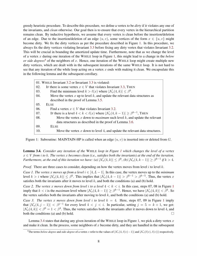
greedy heuristic procedure. To describe this procedure, we define a vertex to be dirty if it violates any one ofthe invariants, and clean otherwise. Our goal then is to ensure that every vertex in the hierarchical partitionremains clean. By inductive hypothesis, we assume that every vertex is clean before the insertion/deletionof an edge. Due to the insertion/deletion of an edge (u, v), some vertices of the form x ∈ u, v mightbecome dirty. We fix the dirty vertices as per the procedure described in Figure 11. In this procedure, wealways fix the dirty vertices violating Invariant 3.33.3 before fixing any dirty vertex that violates Invariant 3.23.2.This will be crucial in bounding the amortized update time. Furthermore, note that as we change the levelof a vertex x during one iteration of the WHILE loop in Figure 11, this might lead to a change in the belowor side degrees44 of the neighbors of x. Hence, one iteration of the WHILE loop might create multiple newdirty vertices, which are dealt with in the subsequent iterations of the same WHILE loop. It is not hard tosee that any iteration of the while loop acting on a vertex x ends with making it clean. We encapsulate thisin the following lemma and the subsequent corollary.

01. WHILE Invariant 3.23.2 or Invariant 3.33.3 is violated:02. IF there is some vertex x ∈ V that violates Invariant 3.33.3, THEN

03. Find the minimum level k > `(x) where |Nx(4, k)| ≤ βk.04. Move the vertex x up to level k, and update the relevant data structures as

described in the proof of Lemma 3.53.5.05. ELSE

06. Find a vertex x ∈ V that violates Invariant 3.23.2.07. IF there is a level 4 < k < `(x) where |Nx(4, k − 1)| ≥ βk−1, THEN

08. Move the vertex x down to maximum such level k, and update the relevantdata structures as described in the proof of Lemma 3.63.6.

09. ELSE

10. Move the vertex x down to level 4, and update the relevant data structures.

Figure 1: Subroutine: MAINTAIN-HP is called when an edge (u, v) is inserted into or deleted from G.

Lemma 3.4. Consider any iteration of the WHILE loop in Figure 11 which changes the level of a vertexx ∈ V from i to k. The vertex x becomes clean (i.e., satisfies both the invariants) at the end of the iteration.Furthermore, at the end of this iteration we have: (a) |Nx(4, k)| ≤ βk, (b) |Nx(4, k − 1)| ≥ βk−1 if k > 4.

Proof. There are three cases to consider, depending on how the vertex moves from level i to level k.

Case 1. The vertex x moves up from a level i ∈ [4, L− 1]. In this case, the vertex moves up to the minimumlevel k > i where |Nx(4, k)| ≤ βk. This implies that |Nx(4, k − 1)| > βk−1 > βk−5. Thus, the vertex xsatisfies both the invariants after it moves to level k, and both the conditions (a) and (b) hold.

Case 2. The vertex x moves down from level i to a level 4 < k < i. In this case, steps 07, 08 in Figure 11imply that k < i is the maximum level where |Nx(4, k − 1)| ≥ βk−1. Hence, we have |Nx(4, k)| < βk. Sothe vertex satisfies both the invariants after moving to level k, and both the conditions (a) and (b) hold.

Case 3. The vertex x moves down from level i to level k = 4. Here, steps 07, 09 in Figure 11 implythat |Nx(4, j − 1)| < βj−1 for every level 4 < j < i. In particular, setting j = 5 = k + 1, we get:|Nx(4, k)| < β0 = 1 < β4. Thus, the vertex satisfies both the invariants after it moves down to level 4, andboth the conditions (a) and (b) hold.

Lemma 3.43.4 states that during any given iteration of the WHILE loop in Figure 11, we pick a dirty vertex xand make it clean. In the process, some neighbors of x become dirty, and they are handled in the subsequent

4The terms below-degree and side-degree of a vertex v refer to the values of |Nv(4, `(v)−1)| and |Nv(`(v), `(v))| respectively.

8

iterations of the same WHILE loop. When the WHILE loop terminates, every vertex is clean by definition.It now remains to analyze the time spent on implementing this WHILE loop after an edge insertion/deletionin the input graph. Lemma 3.43.4 will be crucial in this analysis. The intuition is as follows. The lemmaguarantees that whenever a vertex x moves to a level k > 4, its below-degree is at least βk−1. In contrast,Invariant 3.23.2 and Figure 11 ensure that whenever the vertex moves down from the same level k, its below-degree is less than βk−5. Thus, the vertex loses at least βk−1− βk−5 in below-degree before it moves downfrom level k. This slack of βk−1 − βk−5 help us bound the amortized update time. We next bound the timespent on a single iteration of the WHILE loop in Figure 11.

Lemma 3.5. Consider any iteration of the WHILE loop in Figure 11 where a vertex x moves up to a level kfrom a level i < k (steps 2 – 4). It takes Θ(βk) time to implement such an iteration.

Proof. First, we claim that the value of k (the level where the vertex x will move up to) can be identifiedin Θ(k − i) time. This is because we explicitly store the sizes of the lists Nx(4, i − 1) and Nx(j, j) for allj ≥ i. Next, we update the lists C+

v , Cv and the counters µ+v (c) for x and its neighbors as follows. FOR

every level j ∈ i, . . . , k and every vertex y ∈ Nx(j, j):

• C+y ← C+

y ∪ χ(x), Cy ← Cy \ χ(x) and µ+y (χ(x))← µ+

y (χ(x)) + 1.

• IF j < k, THEN

– µ+x (χ(y))← µ+

x (χ(y))− 1.

– If µ+x (χ(y)) = 0, then C+

x ← C+x \ χ(y) and Cx ← Cx ∪ χ(y).

The time spent on the above operations is bounded by the number of vertices in Nx(4, k).Since the vertex x is moving up from level i to level k > i, we have to update the position of x in the

neighborhood lists of the vertices u ∈ Nx(4, k). We also need to merge the lists Nx(4, i− 1) and Nx(j, j)for i ≤ j < k into a single list Nx(4, k − 1). In the process if some vertices u ∈ Nx(4, k) becomes dirty,then we need to put them in the correct dirty queue. This takes Θ(|Nx(4, k)|) time.

By Lemma 3.43.4, we have |Nx(4, k)| ≤ βk, and |Nx(4, k)| ≥ |Nx(4, k − 1)| ≥ βk−1. Since β is aconstant, we conclude that it takes Θ(βk) time to implement this iteration of the WHILE loop in Figure 11.

Lemma 3.6. Consider any iteration of the WHILE loop in Figure 11 where a vertex x moves down to a levelk from a level i > k (steps 5 – 10). It takes O(βi) time to implement such an iteration.

Proof. We first bound the time spent on identifying the level k < i the vertex x will move down to. Sincethe vertex x violates Invariant 3.23.2, we know that |Nx(4, i− 1)| < βi−5 = O(βi). Therefore, the algorithmcan scan through the list Nx(4, i− 1) and find the required level k in Θ(i+ |Nx(4, i− 1)|) time. Next, weupdate the lists C+

v , Cv and the counters µ+v (c) for x and its neighbors as follows.

FOR every vertex y ∈ Nx(4, i− 1) ∪Nx(i, i):

• IF i ≥ `(y) > k, THEN

– µ+y (χ(x))← µ+

y (χ(x))− 1.

– If µ+y (χ(x)) = 0, then C+

y ← C+y \ χ(x) and Cy ← Cy ∪ χ(x).

• IF i > `(y) ≥ k, THEN

– C+x ← C+

x ∪ χ(y), Cx ← Cx \ χ(y) and µ+x (χ(y))← µ+

x (χ(y)) + 1.

9

The time spent on the above operations is bounded by the number of vertices in Nx(4, i).Since the vertex x is moving down from level i to level k < i, we have to update the position of x in

the neighborhood lists of the vertices u ∈ Nx(4, i). We also need to split the list Nx(4, i − 1) into the listsNx(4, k − 1) and Nx(j, j) for k ≤ j < i. In the process if some vertices u ∈ Nx(4, i) become dirty, thenwe need to put them in the correct dirty queue. This takes Θ(|Nx(4, i)|) time.

Figure 11 ensures that x satisfies Invariant 3.33.3 at level i before it moves down to a lower level. Thus,we have |Nx(4, i)| ≤ βi, and we spend Θ(1 + |Nx(4, i)|) = O(βi) time on this iteration of the WHILE

loop.

Corollary 3.7. It takes Ω(βk) time for a vertex x to move from a level i to a different level k.

Proof. If 4 ≤ i < k, then the corollary follows immediately from Lemma 3.53.5. For the rest of the proof,suppose that i > k. In this case, as per the proof of Lemma 3.63.6, the time spent is at least the size of the listNx(4, k − 1), and Lemma 3.43.4 implies that |Nx(4, k − 1)| ≥ βk−1. Hence, the total time spent is Ω(βk−1),which is also Ω(βk) since β is a constant. Note that we ignored the scenarios where k = 4 since in thatevent βk is a constant anyway.

In Theorem 3.83.8, we bound the amortized update time for maintaining a hierarchical partition.

Theorem 3.8. We can maintain a hierarchical partition of the vertex set V that satisfies Invariants 3.23.2and 3.33.3 in O(log ∆) amortized update time.

We devote the rest of Section 3.23.2 to the proof of the above theorem using a token based scheme. Thebasic framework is as follows. For every edge insertion/deletion in the input graph we create at most O(L)tokens, and we use one token to perform O(β2) units of computation. This implies an amortized updatetime of O(β2 · L) = O(β2 · logβ ∆), which is O(log ∆) since β is a constant.

Specifically, we associate θ(v) many tokens with every vertex v ∈ V and θ(u, v) many tokens with everyedge (u, v) ∈ E in the input graph. The values of these tokens are determined by the following equalities.

θ(u, v) = L−max(`(u), `(v)). (3.1)

θ(v) =max

(0, β`(v)−1 − |Nv(4, `(v)− 1)|

)2β

if `(v) > 4; (3.2)

= 0 otherwise.

Initially, the input graph G is empty, every vertex is at level 4, and θ(v) = 0 for all v ∈ V . Due to theinsertion of an edge (u, v) in G, the total number of tokens increases by at most L−max(`(u), `(v)) < L,where `(u) and `(v) are the levels of the endpoints of the edge just before the insertion. On the other hand,due to the deletion of an edge (u, v) in the input graph, the value of θ(x) for x ∈ u, v increases by atmost 1/(2β), and the tokens associated with the edge (u, v) disappears. Overall, the total number of tokensincreases by at most 1/(2β) + 1/(2β) ≤ O(L) due to the deletion of an edge. We now show that the workdone during one iteration of the WHILE loop in Figure 11 is proportional to O(β2) times the net decreasein the total number of tokens during the same iteration. Accordingly, we focus on any single iteration ofthe WHILE loop in Figure 11 where a vertex x (say) moves from level i to level k. We consider two cases,depending on whether x moves to a higher or a lower level.

Case 1: The vertex x moves up from level i to level k > i. Immediately after the vertex x moves upto level k, we have Nx(4, k − 1) ≥ βk−1 and hence θ(x) = 0. This follows from (3.23.2) and Lemma 3.43.4.Since θ(x) is always nonnegative, the value of θ(x) does not increase as x moves up to level k. We nowfocus on bounding the change in the total number of tokens associated with the neighbors of x. Note

10

that the event of x moving up from level i to level k affects only the tokens associated with the verticesu ∈ Nx(4, k). Specifically, from (3.23.2) we infer that for every vertex u ∈ Nx(4, k), the value of θ(u)increases by at most 1/(2β). On the other hand, for every vertex u ∈ Nx(k + 1, L), the value of θ(u)remains unchanged. Thus, the total number of tokens associated with the neighbors of x increases by atmost (2β)−1 · |Nx(4, k)| ≤ (2β)−1 ·βk = βk−1/2. The inequality follows from Lemma 3.43.4. To summarize,the total number of tokens associated with all the vertices increases by at most βk−1/2.

We now focus on bounding the change in the total number of tokens associated with the edges incidenton x. From (3.13.1) we infer that for every edge (x, u) with u ∈ Nx(4, k − 1), the value of θ(x, u) dropsby at least one as the vertex x moves up from level i < k to level k. For every other edge (x, u) withu ∈ Nx(k, L), the value of θ(x, u) remains unchanged. Overall, this means that the total number of tokensassociated with the edges drops by at least |Nx(4, k− 1)| ≥ βk−1. The inequality follows from Lemma 3.43.4.To summarize, the total number of tokens associated with the edges decreases by at least βk−1.

From the discussion in the preceding two paragraphs, we reach the following conclusion: As the vertexx moves up from level i < k to level k, the total number of tokens associated with all the vertices and edgesdecreases by at least βk−1 − βk−1/2 ≥ βk−1/2. In contrast, Lemma 3.53.5 states that it takes O(βk) timetaken to implement this iteration of the WHILE loop in Figure 11. Hence, we derive that the time spent onupdating the relevant data structures is at most O(2β) = O(β2) times the net decrease in the total numberof tokens. This concludes the proof of Theorem 3.83.8 for Case 1.

Case 2: The vertex x moves down from level i to level k < i. As in Case 1, we begin by observing thatimmediately after the vertex x moves down to level k, we have |Nx(4, k − 1)| ≥ βk−1 if k > 4, and henceθ(x) = 0. This follows from Lemma 3.43.4. The vertex x violates Invariant 3.23.2 just before moving from leveli to level k (see step 6 in Figure 11). In particular, just before the vertex moves down from level i to level k,we have |Nx(4, i − 1)| < βi−5 and θ(x) ≥ (2β)−1 ·

(βi−1 − βi−5

)= βi−2/2 − βi−6/2 ≥ βi−2/3. The

last inequality holds since β is a sufficiently large constant. So the number of tokens associated with x dropsby at least βi−2/3 as it moves down from level i to level k. Also, from (3.23.2) we infer that the value of θ(u)does not increase for any u ∈ Nx as x moves down to a lower level. Hence, we conclude that:

The total number of tokens associated with all the vertices drops by at least βi−2/3. (3.3)

We now focus on bounding the change in the number of tokens associated with the edges incident on x.From (3.13.1) we infer that the number of tokens associated with an edge (u, x) ∈ Nx(4, i − 1) increases by(i − max(k, `(u))) as x moves down from level i to level k. In contrast, the number of tokens associatedwith any other edge (u, x) ∈ Nx(i, L) does not change as the vertex x moves down from level i to a lowerlevel. Let Γ be the increase in the total number of tokens associated with all the edges. Thus, we have:

Γ =∑

(u,x)∈Nx(4,i−1)

(i−max(k, `(u))) =i−1∑j=k

|Nx(4, j)|, (3.4)

where the last equality follows by rearrangement. Next, recall that the vertex x moves down from level i tolevel k during the concerned iteration of the WHILE loop in Figure 11. Accordingly, steps 7 – 10 in Figure 11implies that |Nx(4, j − 1)| < βj−1 for all levels i > j > k. This is equivalent to the following statement:

|Nx(4, j)| < βj for all levels i− 1 > j ≥ k. (3.5)

Next, step 6 in Figure 11 implies that the vertex x violates Invariant 3.23.2 at level i. Thus, we get: |Nx(4, i −1)| < βi−5. Note that for all levels j < i, we haveNx(4, j) ⊆ Nx(4, i−1) and |Nx(4, j)| ≤ |Nx(4, i−1)|.Hence, we get: |Nx(4, j)| < βi−5 for all levels j < i. Combining this observation with (3.53.5), we get:

|Nx(4, j)| < min(βi−5, βj) for all levels i− 1 ≥ j ≥ k. (3.6)

11

Plugging (3.63.6) into (3.43.4), we get:

Γ < 5βi−5 +i−6∑j=k

βj < βi−3. (3.7)

In the above derivation, the last inequality holds since β is a sufficiently large constant.From (3.33.3) and (3.73.7), we reach the following conclusion: As the vertex x moves down from level i to

a level k < i, the total number of tokens associated with all the vertices and edges decreases by at leastβi−2/3−Γ > βi−2/3− βi−3 = Ω(βi−2). In contrast, by Lemma 3.63.6 it takes O(βi) time to implement thisiteration of the WHILE loop in Figure 11. Hence, we derive that the time spent on updating the relevant datastructures is at most O(β2) times the net decrease in the total number of tokens. This concludes the proof ofTheorem 3.83.8 for Case 2.

3.3 The recoloring subroutine.

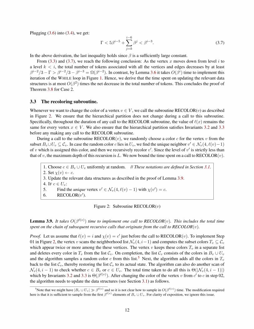
Whenever we want to change the color of a vertex v ∈ V , we call the subroutine RECOLOR(v) as describedin Figure 22. We ensure that the hierarchical partition does not change during a call to this subroutine.Specifically, throughout the duration of any call to the RECOLOR subroutine, the value of `(x) remains thesame for every vertex x ∈ V . We also ensure that the hierarchical partition satisfies Invariants 3.23.2 and 3.33.3before any making any call to the RECOLOR subroutine.

During a call to the subroutine RECOLOR(v), we randomly choose a color c for the vertex v from thesubsetBv∪Uv ⊆ Cv. In case the random color c lies in Uv, we find the unique neighbor v′ ∈ Nv(4, `(v)−1)of v which is assigned this color, and then we recursively recolor v′. Since the level of v′ is strictly less thanthat of v, the maximum depth of this recursion isL. We now bound the time spent on a call to RECOLOR(v).

1. Choose c ∈ Bv ∪ Uv uniformly at random. // These notations are defined in Section 3.13.1.2. Set χ(v)← c.3. Update the relevant data structures as described in the proof of Lemma 3.93.9.4. IF c ∈ Uv:5. Find the unique vertex v′ ∈ Nv(4, `(v)− 1) with χ(v′) = c.6. RECOLOR(v′).

Figure 2: Subroutine RECOLOR(v)

Lemma 3.9. It takes O(β`(v)) time to implement one call to RECOLOR(v). This includes the total timespent on the chain of subsequent recursive calls that originate from the call to RECOLOR(v).

Proof. Let us assume that `(v) = i and χ(v) = c′ just before the call to RECOLOR(v). To implement Step01 in Figure 22, the vertex v scans the neighborhood listNv(4, i−1) and computes the subset colors Tv ⊆ Cvwhich appear twice or more among the these vertices. The vertex v keeps these colors Tv in a separate listand deletes every color in Tv from the list Cv. On completion, the list Cv consists of the colors in Bv ∪ Uvand the algorithm samples a random color c from this list.55 Next, the algorithm adds all the colors in Tvback to the list Cv, thereby restoring the list Cv to its actual state. The algorithm can also do another scan ofNv(4, i − 1) to check whether c ∈ Bv or c ∈ Uv. The total time taken to do all this is Θ(|Nv(4, i − 1)|)which by Invariants 3.23.2 and 3.33.3 is Θ(β`(v)). After changing the color of the vertex v from c′ to c in step 02,the algorithm needs to update the data structures (see Section 3.13.1) as follows.

5Note that we might have |Bv ∪ Uv| β`(v) and so it is not clear how to sample in O(β`(v)) time. The modification requiredhere is that it is sufficient to sample from the first β`(v) elements of Bv ∪ Uv . For clarity of exposition, we ignore this issue.

12

• FOR every vertex w ∈ Nv(4, i):

– µ+w(c′)← µ+

w(c′)− 1.

– IF µ+w(c′) = 0, THEN C+

w ← C+w \ c′ and Cw ← Cw ∪ c′.

– C+w ← C+

w ∪ c, Cw ← Cw \ c and µ+w(c)← µ+

w(c) + 1.

The above operations also take Θ(|Nv(4, i)|) = Θ(β`(v)) time, as per Invariants 3.23.2 and 3.33.3.Finally, in the subsequent recursive calls suppose we recolor the vertices y1, y2, . . .. Note that `(x) >

`(y1) > `(y2) > · · · . Therefore the total time taken can be bounded by Θ(β`(x) +β`(y1) + · · · ) = Θ(β`(x))since it is a geometric series sum. This completes the proof.

3.4 The complete algorithm and analysis.

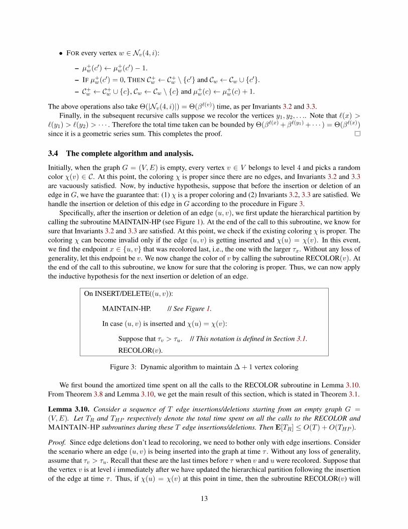
Initially, when the graph G = (V,E) is empty, every vertex v ∈ V belongs to level 4 and picks a randomcolor χ(v) ∈ C. At this point, the coloring χ is proper since there are no edges, and Invariants 3.23.2 and 3.33.3are vacuously satisfied. Now, by inductive hypothesis, suppose that before the insertion or deletion of anedge in G, we have the guarantee that: (1) χ is a proper coloring and (2) Invariants 3.23.2, 3.33.3 are satisfied. Wehandle the insertion or deletion of this edge in G according to the procedure in Figure 33.

Specifically, after the insertion or deletion of an edge (u, v), we first update the hierarchical partition bycalling the subroutine MAINTAIN-HP (see Figure 11). At the end of the call to this subroutine, we know forsure that Invariants 3.23.2 and 3.33.3 are satisfied. At this point, we check if the existing coloring χ is proper. Thecoloring χ can become invalid only if the edge (u, v) is getting inserted and χ(u) = χ(v). In this event,we find the endpoint x ∈ u, v that was recolored last, i.e., the one with the larger τx. Without any loss ofgenerality, let this endpoint be v. We now change the color of v by calling the subroutine RECOLOR(v). Atthe end of the call to this subroutine, we know for sure that the coloring is proper. Thus, we can now applythe inductive hypothesis for the next insertion or deletion of an edge.

On INSERT/DELETE((u, v)):

MAINTAIN-HP. // See Figure 11.

In case (u, v) is inserted and χ(u) = χ(v):

Suppose that τv > τu. // This notation is defined in Section 3.13.1.

RECOLOR(v).

Figure 3: Dynamic algorithm to maintain ∆ + 1 vertex coloring

We first bound the amortized time spent on all the calls to the RECOLOR subroutine in Lemma 3.103.10.From Theorem 3.83.8 and Lemma 3.103.10, we get the main result of this section, which is stated in Theorem 3.13.1.

Lemma 3.10. Consider a sequence of T edge insertions/deletions starting from an empty graph G =(V,E). Let TR and THP respectively denote the total time spent on all the calls to the RECOLOR andMAINTAIN-HP subroutines during these T edge insertions/deletions. Then E[TR] ≤ O(T ) +O(THP ).

Proof. Since edge deletions don’t lead to recoloring, we need to bother only with edge insertions. Considerthe scenario where an edge (u, v) is being inserted into the graph at time τ . Without any loss of generality,assume that τv > τu. Recall that these are the last times before τ when v and uwere recolored. Suppose thatthe vertex v is at level i immediately after we have updated the hierarchical partition following the insertionof the edge at time τ . Thus, if χ(u) = χ(v) at this point in time, then the subroutine RECOLOR(v) will

13

be called to change the color of the endpoint v. On the other hand, if χ(u) 6= χ(v) at this point in time,then no vertex will be recolored. Furthermore, suppose that the vertex v was at level j during the call toRECOLOR(v) at time τv. The analysis is done via three cases.

Case 1: i > j. In this case, at some point in time during the interval [τv, τ ], the subroutine MAINTAIN-HPraised the level of the vertex v to i. Corollary 3.73.7 implies that this takes Ω(βi) time. On the other hand, evenif the subroutine RECOLOR(v) is called at time τ , by Lemma 3.93.9 it takes O(βi) time to implement thatcall. So the total time spent on all such calls to the RECOLOR subroutine is at most O(THP ).

Case 2: 4 < i ≤ j. In this case, we use the fact that the vertex v picks a random color at time τv. In particular,by Lemma 3.93.9 the expected time spent on recoloring the vertex v at time τ is at most O(βi) · Pr[Eτ ], whereEτ is the event that χ(u) = χ(v) just before the insertion at time τ . We wish to bound this probabilityPr[Eτ ], which is evaluated over the past random choices of the algorithm which the adversary fixing theorder of edge insertions is oblivious to.66 We do this by using the principle of deferred decision.

Let cu and cv respectively denote the colors assigned to the vertices u and v during the calls to thesubroutines RECOLOR(u) and RECOLOR(v) at times τu and τv. Note that the event Eτ occurs iff cu = cv.Condition on all the random choices made by the algorithm till just before the time τv. Since τu < τv, thisfixes the color cu. At time τv, the vertex v picks the color cv uniformly at random from the subset of colorsBv ∪ Uv. Let λ denote the size of this subset Bv ∪ Uv at time τv. Clearly, the event cv = cu occurs withprobability 1/λ, i.e., we have Pr[Eτ ] = 1/λ. It now remains to lower bound λ. Since 4 < i ≤ j, Claim 3.13.1and Invariant 3.23.2 imply that when the vertex v gets recolored at time τv, we have: λ = |Bv ∪ Uv| ≥1 + |Nv(4, j − 1)|/2 ≥ 1 + βj−5/2 = Ω(βj−5) = Ω(βi−5). To summarize, the expected time spent onthe possible call to RECOLOR(v) at time τ is at most O(βi) · Pr[Eτ ] = O(βi) · (1/λ) = O(β5) = O(1).Hence, the total time spent on all such calls to the RECOLOR subroutine is at most O(T ).

Case 3. i = 4. Even if RECOLOR(v) is called at time τ , by Lemma 3.93.9 at most O(β4) = O(1) time isspent on that call. So the total time spent on all such calls to the RECOLOR subroutine is O(T ).

Proof of Theorem 3.13.1. The theorem holds since E[TR]+THP ≤ O(T )+O(THP ) ≤ O(T )+O(T log ∆) =O(T log ∆). The first and the second inequalities respectively follow from Lemma 3.103.10 and Theorem 3.83.8.

4 A Deterministic Dynamic Algorithm for (1 + o(1))∆ Vertex Coloring

Let G = (V,E) denote the input graph that is changing dynamically, and let ∆ be an upper bound on themaximum degree of any vertex in G. For now we assume that the value of ∆ does not change with time. InSection 66, we explain how to relax this assumption. Our main result is stated in the theorem below.

Theorem 4.1. We can maintain a (1 + o(1))∆ vertex coloring in a dynamic graph deterministically inO(lg5+o(1) ∆/ lg lg2 ∆) amortized update time.

4.1 Notations and preliminaries.

Throughout Section 44, we define three parameters η, L, λ as follows.

η = e16/ lg lg ∆, L =

⌊lg(η∆)

lg lg ∆

⌋and λ =

⌈2

lg(η∆)L

⌉. (4.1)

We will use λL colors. From (4.14.1) and Lemma 4.24.2, it follows that λL ≤ η∆ = (1 + o(1))∆ when∆ = ω(1). In Lemma 4.24.2, we establish a couple of useful bounds on the parameters η, L and λ.

6In case 1, we used the trivial upper bound Pr[Eτ ] ≤ 1.

14

Lemma 4.2. We have:

1. lg ∆ ≤ λ ≤ 2 lg1+o(1) ∆, and

2. λL ≤ η∆ ≤ (λ+ 1)L.

Proof. From (4.14.1) we infer that:

λ ≥ 2lg(η∆)L ≥ 2

lg(η∆)lg(η∆)/ lg lg ∆ = lg ∆.

From (4.14.1) we also infer that:

λ ≤ 2 · 2lg(η∆)L

≤ 2 · 2lg(η∆)

lg(η∆)/ lg lg ∆−1

= 2 · 2lg(η∆)

lg(η∆)−lg lg ∆·lg lg ∆

= 2 · 2(1+o(1))·lg lg ∆ = 2 lg1+o(1) ∆.

The proves part (1) of the lemma. Next, note that:

λL ≤(

2lg(η∆)L

)L= η∆ ≤

⌈2

lg(η∆)L

⌉L= (λ+ 1)L.

This proves part (2) of the lemma.

We let C = 1, . . . , λL denote the palette of all colors. Note that |C| = λL = (1 + o(1))∆. Indeed,we view the colors available to us as L-tupled vectors where each coordinate takes one of the values from1, . . . , λ. In particular, the color assigned to any vertex v is denotes as χ(v) = (χ1(v), . . . , χL(v)), whereχi(v) ∈ [λ] for each i ∈ [L]. Given such a coloring χ : V → C, for every index i ∈ [L] we define χ∗i (v) :=(χ1(v), . . . , χi(v)) to be the i-tuple denoting the first i coordinates of χ(v). For notational convenience, wedefine χ∗0(v) := ⊥ for all v. For all i ∈ [L] and α ∈ [λ], we let χ∗i→α(v) = (χ1(v), . . . , χi−1(v), α) denotethe i-tuple whose first (i− 1) coordinates are the same as that of χ but whose ith coordinate is α.

For all i ∈ [L] and α ∈ [λ], we define the subsets N∗i (v) = u ∈ V : (u, v) ∈ E and χ∗i (u) = χ∗i (v)and N∗i→α(v) = u ∈ V : (u, v) ∈ E and χ∗i (u) = χ∗i→α(v). In other words, the set N∗i (v) consists ofall the neighbors of a vertex v ∈ V whose colors have the same first i coordinates as the color of v. On theother hand, the set N∗i→α(v) denotes the status of the set N∗i in the event that the vertex v decides to changethe ith coordinate of its color to α. In particular, if χi(v) 6= α, then N∗i (v) ∩N∗i→α(v) = ∅. Going over allpossible choices of χi(v) we get the following

N∗i−1(v) =⋃α∈[λ]

N∗i→α(v)

Also note that N∗0 (v) is the full neighborhood of v. Define D∗i (v) = |N∗i (v)| and D∗i→α(v) = |N∗i→α(v)|.The above observations is encapsulated in the following corollary.

Corollary 4.3. For every vertex v ∈ V , and every index j ∈ 1, . . . , L, the set N∗j−1(v) is partitioned intothe subsets N∗j→α(v) for α ∈ 1, . . . , λ. In particular, we have: D∗j−1(v) =

∑α∈[λ]D

∗j→α(v).

We maintain the following invariant.

Invariant 4.4. For all v ∈ V , i ∈ [0, L], we have D∗i (v) ≤ (∆/λi) · f(i), where f(i) = ((λ+ 1)/(λ−1))i.

15

For every j, we have f(j) > 1 and f(j − 1) ≤ f(j). We now give a brief intuitive explanation forthe above invariant. Associate a rooted λ-ary tree Tv of depth L with every vertex v ∈ V . We shall referto the vertices of this tree Tv as meta-vertices, to distinguish them from the vertices of the input graphG = (V,E). The total number of leaves in this tree is λL, which is the same as the total number availablecolors. Thus, we can ensure that each root to leaf path in this tree corresponds to a color in a natural way,and any internal meta-vertex at depth i corresponds to the ith coordinate of a color. The quantity D∗i (v) cannow be interpreted as follows. Consider the meta-vertex (say) xi at depth i on the unique root to leaf pathcorresponding to the color of v. Let µi denote the number of all neighbors of v in G such that this meta-vertex xi also belongs to the root to leaf paths for their corresponding colors. Then we have D∗i (v) = µi.Note that if i = 0, then the meta-vertex xi is the root of the tree, which is at depth zero. It follows that ifi = 0, then µi equals the degree of the vertex v in the input graph G, which is at most ∆. Thus, we haveµ0 ≤ ∆. Now, let y1, . . . , yλ denote the children of the root x0 in this λ-ary tree Tv. A simple countingargument implies that there exists an index j ∈ 1, . . . , λ with the following property: At most a 1/λfraction of the neighbors of v in G have colors whose corresponding root to leaf paths contain the meta-vertex yj . Thus, if it were the case that the root to leaf path corresponding to the color of v also passesthrough such a meta-vertex yj , then we would have D∗i (v) = µi ≤ ∆/λ for i = 1. Invariant 4.44.4, on theother hand, gives a slack of f(1) and requires that D∗i (v) ≤ (∆/λ) · f(1) for i = 1. We can interpretthe invariant in this fashion for every subsequent index i ∈ 2, . . . , L by iteratively applying the sameprinciple. The reader might find it helpful to keep this interpretation in mind while going through the formaldescription of the algorithm and its analysis.

Lemma 4.5. If Invariant 4.44.4 holds then χ is a proper vertex coloring.

Proof. Claim 4.14.1 implies that for i = L, the invariant reduces to: D∗L(v) < 1. Since D∗L(v) is a nonnegativeinteger, we get D∗L(v) = 0. Since D∗L(v) is the number of neighbors of v who are assigned the color χ(v),no two adjacent vertices can get the same color. The invariant thus ensures a proper vertex coloring.

Claim 4.1. We have: (∆/λL) · f(L) < 1.

In order to prove Claim 4.14.1, we derive that:

(∆/λL)f(L)

≤ (((λ+ 1)L/η)/λL) · f(L) (4.2)

= (1/η) · (1 + 1/λ)L · (1 + 2/(λ− 1))L

≤ (1/η) · (1 + 1/λ)L · (1 + 4/λ)L (4.3)

≤ (1/η) · (1 + 7/λ)L (4.4)

≤ (1/η) · e7L/λ

≤ (1/η) · e7 lg(η∆)/(λ lg lg ∆) (4.5)

≤ (1/η) · e7 lg(∆2)/(lg ∆ lg lg ∆) (4.6)

≤ (1/η) · e14/ lg lg ∆

< 1. (4.7)

Step (4.24.2) follows from part (2) of Lemma 4.24.2. Steps (4.34.3), (4.44.4) hold as long as λ ≥ 2.77 Step (4.54.5) followsfrom (4.14.1). Step (4.64.6) follows from (4.14.1) and part (1) of Lemma (4.24.2). Step (4.74.7) follows from (4.14.1).

Data structures. For every vertex v ∈ V , our dynamic algorithm maintains the following data structures.7When λ < 2, we have ∆ = O(1) and so we can trivially maintain a (∆ + 1)-vertex coloring in O(∆) = O(1) update time.

16

• For all i ∈ [0, L], the set N∗i (v) as a doubly linked list and the counter D∗i (v). It will be the re-sponsibility of the neighbors of v to update the list N∗i (v) when they change their own colors. Usingappropriate pointers, we will ensure that any given node x can be inserted into or deleted from anygiven list N∗i (y) in O(1) time. Note that each vertex figures out if it satisfies the Invariant 4.44.4 or not.

• The color χ(v) = (χ1(v), . . . , χL(v)) assigned to the vertex v.

4.2 The algorithm.

Initially, since the edge-set of the input graph is empty, we can assign each vertex an arbitrary color. Forconcreteness, we set χi(v) = 1 for all i ∈ [L] and v ∈ V . Since there are no edges, D∗i (v) = 0 for all i, vand so Invariant 4.44.4 vacuously holds at this point. We show how to ensure that the invariant continues toremain satisfied even after any edge insertion or deletion, and bound the amortized update time.

Deletion of an edge. Suppose that an edge (u, v) gets deleted from G. No vertex changes its color due tothis deletion. We only need to update the relevant data structures. Without any loss of generality, supposethat i ∈ [0, L] is the largest index for which we have χ∗i (v) = χ∗i (u). Then for every vertex x ∈ u, vand every j ∈ [0, i], we delete the vertex y ∈ u, v \ x from the set N∗i (x) and decrement the valueof the counter D∗j (x) by one. This takes O(L) time. To summarize, deletion of an edge can be handled inO(L) worst case update time. If Invariant 4.44.4 was satisfied just before the edge deletion, then the invariantcontinues to remain satisfied after the edge deletion since the LHS of the invariant can only decrease.

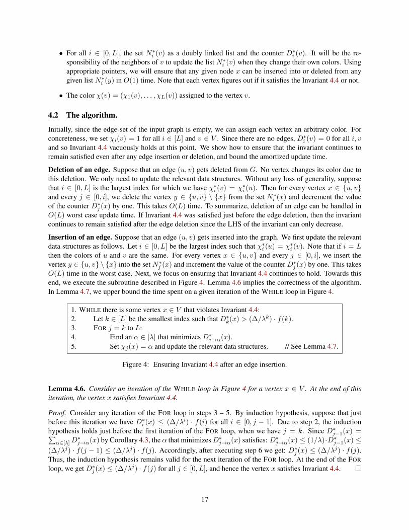
Insertion of an edge. Suppose that an edge (u, v) gets inserted into the graph. We first update the relevantdata structures as follows. Let i ∈ [0, L] be the largest index such that χ∗i (u) = χ∗i (v). Note that if i = Lthen the colors of u and v are the same. For every vertex x ∈ u, v and every j ∈ [0, i], we insert thevertex y ∈ u, v \ x into the set N∗j (x) and increment the value of the counter D∗j (x) by one. This takesO(L) time in the worst case. Next, we focus on ensuring that Invariant 4.44.4 continues to hold. Towards thisend, we execute the subroutine described in Figure 44. Lemma 4.64.6 implies the correctness of the algorithm.In Lemma 4.74.7, we upper bound the time spent on a given iteration of the WHILE loop in Figure 44.

1. WHILE there is some vertex x ∈ V that violates Invariant 4.44.4:2. Let k ∈ [L] be the smallest index such that D∗k(x) > (∆/λk) · f(k).3. FOR j = k to L:4. Find an α ∈ [λ] that minimizes D∗j→α(x).5. Set χj(x) = α and update the relevant data structures. // See Lemma 4.74.7.

Figure 4: Ensuring Invariant 4.44.4 after an edge insertion.

Lemma 4.6. Consider an iteration of the WHILE loop in Figure 44 for a vertex x ∈ V . At the end of thisiteration, the vertex x satisfies Invariant 4.44.4.

Proof. Consider any iteration of the FOR loop in steps 3 – 5. By induction hypothesis, suppose that justbefore this iteration we have D∗i (x) ≤ (∆/λi) · f(i) for all i ∈ [0, j − 1]. Due to step 2, the inductionhypothesis holds just before the first iteration of the FOR loop, when we have j = k. Since D∗j−1(x) =∑

α∈[λ]D∗j→α(x) by Corollary 4.34.3, the α that minimizesD∗j→α(x) satisfies: D∗j→α(x) ≤ (1/λ)·D∗j−1(x) ≤

(∆/λj) · f(j − 1) ≤ (∆/λj) · f(j). Accordingly, after executing step 6 we get: D∗j (x) ≤ (∆/λj) · f(j).Thus, the induction hypothesis remains valid for the next iteration of the FOR loop. At the end of the FOR

loop, we get D∗j (x) ≤ (∆/λj) · f(j) for all j ∈ [0, L], and hence the vertex x satisfies Invariant 4.44.4.

17

Lemma 4.7. It takes O(L · λ+ L · ∆λk−1 · f(k − 1)) time for one iteration of the WHILE loop in Figure 44,

where k is defined as per Step 2 in Figure 44.

Proof. Consider any iteration of the WHILE loop that changes the color of a vertex x ∈ V . Since we storethe value of D∗j (x) for every j ∈ [0, L], it takes O(L) time to find the index k ∈ [0, L] as defined in step 2 ofFigure 44. Next, for every index j ∈ [k, L] and every vertex u ∈ N∗j (x), we set N∗j (u) = N∗j (u) \ x andD∗j (u) = D∗j (u)− 1. Since the vertex x is going to change the kth coordinate of its color, the previous stepis necessary to ensure that no vertex u mistakenly continues to include x in the set N∗j (u) for j ∈ [k, L].This takes O(

∑Lj=k |N∗j (x)|) time. Since N∗j (x) ⊆ N∗j−1(x) for all j ∈ [k, L], the time taken is actually

O((L−k−1) · |N∗k−1(x)|) = O(L · (∆/λk−1) ·f(k−1)). The last equality follows from step 2 in Figure 44.At this point, we also set N∗j (x) = ∅ and D∗j (x) = 0 for all j ∈ [k, L]. We shall rebuild the sets N∗j (x)during the FOR loop in steps 3 - 5. Applying a similar argument as before, we conclude that this also takesO(L · (∆/λk−1) · f(k − 1)) time. It now remains to bound the time spent on the FOR loop.

Consider any iteration of the FOR loop as described by steps 3 - 5 in Figure 44. By inductive hypothesis,suppose that for every index i ∈ [0, j − 1] and every vertex v ∈ V , the list N∗i (v) is now consistentwith the changes we have made to the color of x in the earlier iterations of the FOR loop. Our first goalis to compute the index α ∈ [λ], which we do by scanning the vertices u ∈ N∗j−1(x). In the beginningof this scan, we initialize a counter Zα = 0 for every α ∈ [λ]. Subsequently, while considering anyvertex u ∈ N∗j−1(x) during the scan, we set Zcj(u) = Zcj(u) + 1. At the end of the scan, we returnthe index α ∈ [λ] that minimizes the value of Zα. Thus, overall it takes O(λ + |N∗j−1(x)|) time to findthe index α. Next, for every vertex u ∈ N∗j−1(x) with cj(u) = α, we set N∗j (u) = N∗j (u) ∪ x,N∗j (x) = N∗j (x) ∪ u, D∗j (u) = D∗j (u) + 1 and D∗j (x) = D∗j (x) + 1. It takes O(|N∗j−1(x)|) timeto implement this step. Now, we set cj(x) = α in O(1) time. At this stage, we have updated all therelevant data structures for the index j and changed the jth coordinate of the color of x. This concludes theconcerned iteration of the FOR loop. Since N∗j−1(x) ⊆ N∗k−1(x), the total time spent on this iteration isO(λ+ |N∗j−1(x)|) = O(λ+ |N∗k−1(x)|) = O(λ+ (∆/λk−1) · f(k − 1)), as per step 2 in Figure 44.

Since the FOR loop runs for at most L iterations, the total time spent on the FOR loop is at most O(L ·λ+L · ∆

λk−1 ·f(k−1)). Combining this with the discussion in the first paragraph of the proof of this lemma,we infer that the total time spent on one iteration of the WHILE loop is alsoO(L ·λ+L · ∆

λk−1 ·f(k−1)).

4.3 Bounding the amortized update time.

In this section, we prove Theorem 4.14.1 by bounding the amortized update time of the algorithm described inSection 4.24.2. Recall that handling the deletion of an edge takes O(L) time in the worst case. Furthermore,ignoring the time spent on the WHILE loop in Figure 44, handling the insertion of an edge also takes O(L)time in the worst case. From Lemma 4.24.2 we have L = O(lg ∆/ lg lg ∆). Thus, it remains to bound the timespent on the WHILE loop in Figure 44. We focus on this task for the remainder of this section.

The main idea is the following: by Lemma 4.74.7 the WHILE loop processing vertex x takes a long timewhen k is small which in turn impliesD∗k(x) is large. However, in the FOR loop we choose the colors whichminimize precisely the values of D∗j→α(x). Therefore these quantities cannot be large too often.

Consider any iteration of the WHILE loop in Figure 44, which changes the color of a vertex x ∈ V . LetS+x (resp. S−x ) be the set of all ordered pairs (i, v) such that the value of D∗i (v) increases (resp. decreases)

due to this iteration. The following lemma precisely bounds the increases and decreases of these D∗ values.

Lemma 4.8. During any single iteration of the WHILE loop in Figure 44, we have:

|S−x | > (∆/λk) · f(k) and |S+x | < (∆/λk) · f(k − 1) · λ/(λ− 1).

18

Proof. Throughout the proof, we let t− and t+ respectively denote the time-instant just before and justafter the concerned iteration of the WHILE loop. Let k ∈ [L] be the smallest index such that D∗k(x) >(∆/λk) · f(k) at time t−. For every index j ∈ [0, L] and every vertex v ∈ V , let N∗j (v, t−) and N∗j (v, t+)respectively denote the set of vertices in N∗j (v) at time t− and at time t+.

Consider any vertex u ∈ N∗k (x, t−). At time t−, we had χ∗k(u) = χ∗k(x). The concerned iteration ofthe WHILE loop changes the kth coordinate of the color of x, but the vertex u does not change its colorduring this iteration. Thus, we have χ∗k(u) 6= χ∗k(x) at time t+. We therefore infer that x ∈ N∗k (u, t−)and x /∈ N∗k (u, t+). Hence, for every vertex u ∈ N∗k (x, t−), the value of D∗k(u) drops by one due tothe concerned iteration of the WHILE loop. It follows that (k, u)|u ∈ N∗k (x, t−) ⊆ S−x , and we get:|S−x | ≥ |N∗k (x, t−)| > (∆/λk) · f(k). The last inequality follows from step 2 in Figure 44. This gives us thedesired lower bound on the size of the set S−x . It now remains to upper bound the size of the set S+

x .Consider any ordered pair (j, u) ∈ S+

x . Since the concerned iteration of the WHILE loop increases thevalue of D∗j (u) and does not change the color of any vertex other than x, we infer that:

x /∈ N∗j (u, t−) and x ∈ N∗j (u, t+). (4.8)

The concerned iteration of the WHILE loop does not change the ith coordinate of the color of x for anyi < k. Thus, the i-tuple χ∗i (x) does not change from time t− to time t+. Furthermore, the vertex u does notchange its color during the time-interval [t−, t+]. It follows that if x /∈ N∗i (u, t−) for some i < k, then wealso have x /∈ N∗i (u, t+). From (4.84.8) we therefore get j ∈ [k, L]. Next, note that since x ∈ N∗j (u, t+), wehave χ∗j (x) = χ∗j (u) at time t+, and accordingly we also have u ∈ N∗j (x, t+). To summarize, if an orderedpair (j, u) belongs to the set S+

x , then we must have j ∈ [k, L] and u ∈ N∗j (x, t+). Thus, we get:

|S+x | ≤

L∑j=k

|N∗j (x, t+)| (4.9)

Note that step 4 in Figure 44 picks an α ∈ [λ] that minimizesD∗j→α(x). This gives us the following guarantee.

|N∗k (x, t+)| ≤ |N∗k−1(x, t−)|/λ. (4.10)

|N∗j (x, t+)| ≤ |N∗j−1(x, t+)|/λ for all j ∈ [k + 1, L]. (4.11)

Using (4.94.9), (4.104.10) and (4.114.11), we can upper bound |S+x | by the sum of a geometric series, and get:

|S+x | ≤

L∑j=k

|N∗j (x, t+)|

≤ |N∗k−1(x, t−)| ·(

1

λ+ · · ·+ 1

λL−k+1

)≤ |N∗k−1(x, t−)| · 1

(λ− 1)

≤ ∆

λk−1· f(k − 1) · 1

(λ− 1)

The last inequality holds due to step 2 in Figure 44. This gives us the desired upper bound on |S+x |.

We now use a potential function based argument to prove Theorem 4.14.1, where the potential associatedwith the graph at any point in time is given by Φ =

∑v∈V,i∈[0,L]D

∗i (v). Note that the potential Φ is always

nonnegative. The bound on the amortized update now follows from the three observations stated below.

19

Observation 4.9. Due to the insertion or deletion of an edge inG, the potential Φ changes by at mostO(L).

Proof. Consider the insertion or deletion of an edge (u, v) in the input graph G = (V,E). For all x ∈V \ u, v and i ∈ [0, L], the value of D∗i (x) remains unchanged. Furthermore, for all x ∈ u, v andi ∈ [0, L], the value ofD∗i (x) changes by at most one. Hence, the potential changes by at most 2(L+1).

Observation 4.10. Due to one iteration of the WHILE loop in Figure 44, the potential Φ decreases by at leastΓ = (∆/λk) · f(k − 1)/(λ− 1), where k is defined as per Step 2 in Figure 44.

Proof. Note that the concerned iteration of the WHILE loop does not change the color of any vertex v 6= x.Thus, for every vertex v ∈ V and every index i ∈ [0, L], the value of D∗i (v) changes by at most one. As inLemma 4.84.8, let S+

x (resp. S−x ) denote the set of all ordered pairs (i, v) such that the value ofD∗i (v) increases(resp. decreases) due to this iteration. We therefore infer that the net decrease in Φ is equal to |S−x | − |S+

x |,and we have:

|S−x | − |S+x | ≥ (∆/λk) · f(k)− (∆/λk) · f(k − 1) · λ/(λ− 1)

= (∆/λk) · f(k − 1) · ((λ+ 1)/(λ− 1)− λ/(λ− 1))

= (∆/λk) · f(k − 1)/(λ− 1).

The first step in the above derivation follows from Lemma 4.84.8, and the second step follows from Invari-ant 4.44.4.

Observation 4.11. The time taken to implement one iteration of the WHILE loop in Figure 44 is O((λ− 1) ·λ2 · L · Γ), where Γ is the net decrease in the potential due to the same iteration of the WHILE loop.

Proof. This follows from Observation 4.104.10 and Lemma 4.74.7.

Proof of Theorem 4.14.1. In the beginning when the edge set is empty we have Φ = 0. After T edge insertionsand deletions, the total time taken by the algorithm is O(LT ) +W , where W is the total time taken by theWHILE loops. From Observation 4.114.11 we know that W = O(λ3L ·

∑t Γt), where Γt is the decrease in the

potential due to the tth WHILE loop. On the other hand, from Observation 4.94.9 we get∑

t Γt = O(TL).Putting it all together, we get that the total time taken by the algorithm is O(λ3L2T ). This proves thetheorem since λ = O(log1+o(1) ∆) and L = O(log ∆/ log log ∆) as per (4.14.1) and part (1) of Lemma 4.24.2.

5 A Deterministic Dynamic Algorithm for (2∆− 1) Edge Coloring

Let G = (V,E) be the input graph that is changing dynamically, and let ∆ be an upper bound on themaximum degree of any vertex in G. For now we assume that the value of ∆ does not change with time. InSection 66, we explain how to relax this assumption. We present a simple, deterministic dynamic algorithmfor maintaining a 2∆− 1 edge coloring algorithm in G.

Data Structures. For every vertex v ∈ V , we maintain the following data structures.

1. An array Cv of length 2∆ − 1. Each entry in this array corresponds to a color. For each color c, theentry Cv[c] is either null or points to the unique edge incident on v which is colored c.

2. A bit vector Av of length 2∆− 1, where Av[c] = 0 iff Cv[c] is null, and Av[c] = 1 otherwise.

3. A balanced binary search tree Tv with 2∆ − 1 leaves. We refer to the vertices in the tree as meta-nodes, to distinguish them from the vertices in the input graph G. We maintain a counter val(Tv, x)at every meta-node x in the tree Tv. The value of this counter at the cth leaf of Tv is given by Av[c].Furthermore, the value of this counter at any internal meta-node x of Tv is given by: val(Tv, x) =∑

c:c is a leaf in the subtree rooted at x val(Tv, c).

20

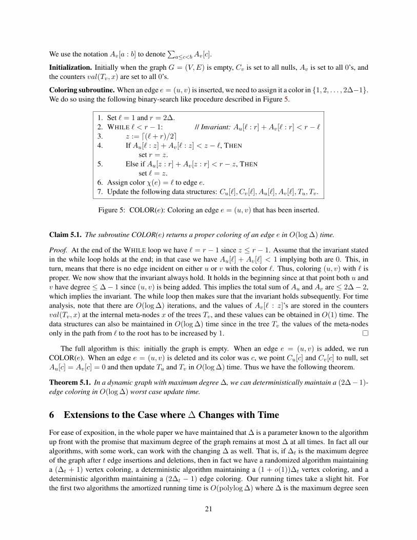
We use the notation Av[a : b] to denote∑

a≤c<bAv[c].

Initialization. Initially when the graph G = (V,E) is empty, Cv is set to all nulls, Av is set to all 0’s, andthe counters val(Tv, x) are set to all 0’s.

Coloring subroutine. When an edge e = (u, v) is inserted, we need to assign it a color in 1, 2, . . . , 2∆−1.We do so using the following binary-search like procedure described in Figure 55.

1. Set ` = 1 and r = 2∆.2. WHILE ` < r − 1: // Invariant: Au[` : r] +Av[` : r] < r − `3. z := d(`+ r)/2e4. If Au[` : z] +Av[` : z] < z − `, THEN

set r = z.5. Else if Au[z : r] +Av[z : r] < r − z, THEN

set ` = z.6. Assign color χ(e) = ` to edge e.7. Update the following data structures: Cu[`], Cv[`], Au[`], Av[`], Tu, Tv.

Figure 5: COLOR(e): Coloring an edge e = (u, v) that has been inserted.

Claim 5.1. The subroutine COLOR(e) returns a proper coloring of an edge e in O(log ∆) time.

Proof. At the end of the WHILE loop we have ` = r − 1 since z ≤ r − 1. Assume that the invariant statedin the while loop holds at the end; in that case we have Au[`] + Av[`] < 1 implying both are 0. This, inturn, means that there is no edge incident on either u or v with the color `. Thus, coloring (u, v) with ` isproper. We now show that the invariant always hold. It holds in the beginning since at that point both u andv have degree ≤ ∆− 1 since (u, v) is being added. This implies the total sum of Au and Av are ≤ 2∆− 2,which implies the invariant. The while loop then makes sure that the invariant holds subsequently. For timeanalysis, note that there are O(log ∆) iterations, and the values of Av[` : z]’s are stored in the countersval(Tv, x) at the internal meta-nodes x of the trees Tv, and these values can be obtained in O(1) time. Thedata structures can also be maintained in O(log ∆) time since in the tree Tv the values of the meta-nodesonly in the path from ` to the root has to be increased by 1.

The full algorithm is this: initially the graph is empty. When an edge e = (u, v) is added, we runCOLOR(e). When an edge e = (u, v) is deleted and its color was c, we point Cu[c] and Cv[c] to null, setAu[c] = Av[c] = 0 and then update Tu and Tv in O(log ∆) time. Thus we have the following theorem.

Theorem 5.1. In a dynamic graph with maximum degree ∆, we can deterministically maintain a (2∆− 1)-edge coloring in O(log ∆) worst case update time.

6 Extensions to the Case where ∆ Changes with Time

For ease of exposition, in the whole paper we have maintained that ∆ is a parameter known to the algorithmup front with the promise that maximum degree of the graph remains at most ∆ at all times. In fact all ouralgorithms, with some work, can work with the changing ∆ as well. That is, if ∆t is the maximum degreeof the graph after t edge insertions and deletions, then in fact we have a randomized algorithm maintaininga (∆t + 1) vertex coloring, a deterministic algorithm maintaining a (1 + o(1))∆t vertex coloring, and adeterministic algorithm maintaining a (2∆t − 1) edge coloring. Our running times take a slight hit. Forthe first two algorithms the amortized running time is O(polylog ∆) where ∆ is the maximum degree seen

21

so far (till time t); for the edge coloring the worst case update time becomes O(log ∆t). In the followingthree subsections we give a brief sketch of the differences in the algorithm and how the analysis needs to bemodified. In all cases, we achieve this by making the requirement on the algorithm stronger.

6.1 Randomized (∆t + 1) vertex coloring.

Let Dv = |Nv(4, L)| be the degree of a vertex v ∈ V in the current input graph. To extend our dynamicalgorithm in Section 33 to the scenario where ∆ changes with time, we simply ensure that the followingproperty holds.

Property 6.1. Every vertex v to have a color χ(v) ∈ 1, . . . , Dv + 1.

To see why it is easy to ensure Property 6.16.1, we only need to make the following two observations.

1. The algorithm that maintains the hierarchical partition in Section 3.23.2 is oblivious to the value of ∆.

2. For every vertex v ∈ V , change the definition of the subset of colors Cv ⊆ C as follows. Now, thesubset Cv ⊆ C consists of all the colors in 1, . . . , Dv+1 that are not assigned to any neighbor u of vwith `(u) ≥ `(v). We can maintain these modified sets Cv by incurring only a O(1) factor cost in theupdate time. Finally, note that even with this modified definition, Claim 3.13.1 continues to hold. Hence,the RECOLOR subroutine in Figure 22 in particular and our randomized dynamic coloring algorithmin general continue to remain valid.

6.2 Deterministic (1 + o(1))∆t vertex coloring.

Whenever degt(v) is less than a (very) large constant, whenever we need to change its color we do thegreedy step taking degt(v) = O(1) time to find a free color. Henceforth assume degt(v) = ω(1). Insteadof having a fixed λ, L and η, for every vertex v we have separate parameters which depend on the degree ofv at time t. Note these can be maintained at each insertion and deletion with O(1) time per update.

ηt(v) := e16

lg lg degt(v) , Lt(v) :=

⌊lg(ηt(v) · degt(v))

lg lg degt(v)

⌋and λt(v) :=

⌈2

lg(ηt(v)·degt(v))Lt(v)

⌉.

At time t, each vertex is assigned a color from 1, 2, . . . , λt(v)Lt(v). As before, this color χ(v) isassumed to be a Lt(v)-dimensional tuple where each entry takes positive integer values in [λt(v)]. Note thatthe dimension of tuple and the range of each dimension of the tuple can change with time and we need to becareful about that. The definitions of N∗i (v) and D∗i (v) remains the same, except that the range of i is nowonly till Lt(v).

The invariant that we maintain for every vertex is similar to Invariant 4.44.4 changed appropriately and weadd the condition that at time t each coordinate is in [λt(v)].

Invariant 6.2. For all t, for all v ∈ V , i ∈ [0, Lt(v)], we have (1) D∗i (v) ≤ (degt(v)/λt(v)i) · ft,v(i),where ft,v(i) = ((λt(v) + 1)/(λt(v)− 1))i, and (2) χ(t)

i (v) ∈ 1, 2, . . . , λt(v).

Let us take care of situations when part (2) of the above invariant is violated because the other part issimilar to as done in Section 44. To do so, for a positive integer p, define dp to be the largest value of degt(v)for which λt(v) evaluates to p. By the definition of the parameters (since λt(v) = Θ(lg degt(v))) we getdp+1 − dp = Θ(dp). To take care of part (2) of Invariant 6.26.2, the algorithm given in Figure 44 needs to bechanged in Step 4 as follows: if degt(v) ∈ [dp, dp+1] (and therefore λt(v) = p + 1), we search for α in[λt(v)] if degt(v) > dp + (dp+1 − dp)/2, otherwise we search for α in [λt(v)− 1].

22

Whenever part (2) of Invariant 6.26.2 is violated by vertex v at time t, we perform the following changes.We take Θ(degt(v)) time to find a color for v such that χi(v) ∈ [λt(v)] for all i ∈ [Lt(v)] satisfyingInvariant 6.26.2. We now show that this time can be charged to edge deletions incident on v that has happenedin the past, and furthermore these edge deletions will not be charged to again.

Firstly note that v violated part (2) on Invariant 6.26.2 only because we delete an edge (u, v) and degt(v)

and therefore λt(v) has gone down. Note that it must be the case χ(t)i (v) = λt(v) + 1 = λt−(v), where

the third term is the value of λt(v) just before the edge deletion. Suppose λt(v) = p. Note that degt(v)must be dp since at time degt−(v) = degt(v) + 1 and λt−(v) = p + 1. Look at the last time t′ before tat which χ(t′)

i (v) was set to p + 1. At that time, because of the modification made above to the algorithm,we must have had degt′(v) > dp + (dp+1 − dp)/2. Therefore between t′ and t we must have had at least(dp+1 − dp)/2 = Θ(dp) = Θ(degt(v)) edge deletions incident on v. We charge the Θ(degt(v)) time takento recolor v due to violation of part (2) of invariant to these deletions. Note that since we choose t′ to be thelast time before t, we won’t charge to these edge deletions again.

To maintain part (1) of the invariant, the algorithm is similar as in the previous section with two changes:(1) firstly, the WHILE loop checks the new invariant, and (2) is the technical change described above.Observe that even when we delete an edge we run the risk of the invariant getting violated since the RHSof the invariant also goes down. For the analysis, the one line argument why everything generalizes isthat our analysis is in fact vertex -by-vertex. More precisely, we have a version of Lemma 4.74.7 where the∆, L, λ, f are replaced by degt(v), Lt(v), λt(v), ft,v. Similar changes are in all the other claims and lemmasand for brevity we don’t mention the subscripts below. For instance, time analysis of Lemma 4.74.7 for theWHILE loop taking care of vertex x generalizes with Lt(x), λt(x), ft,x and degt(x) replacing L, λ, f and∆. Similarly, in Lemma 4.84.8 we have exactly the same changes which reflects in Observation 4.104.10. That is,the decrease in potential in a single while loop is charged to the running time of that while loop. The rest ofthe analysis as in Section 44. There is an extra change in Lemma 4.84.8 where because of the technical changewe made, we only get |S+

x | < (∆/λk) · f(k − 1) · λ/(λ − 2) since we could be searching over a range of[λ− 1]. This only increases the update time by an extra factor which is O(1) if λ ≥ 2.

6.3 Deterministic (2∆t − 1) edge coloring.

We assert the invariant that every edge (u, v) gets a color from the palette 1, . . . , 2 max(degt(u), degt(v))−1. In the subroutine COLOR(e), the upper bound u is then set to u = degt(u) + degt(v), and the rest ofthe algorithm remains the same. The trees Tu and Tv now need to be dynamically balanced; but this can bedone in O(log ∆t) time using say red-black trees. The other place where the algorithm needs to change isthat when an edge e = (u, v) is deleted, the degree of both u and v go down. That may lead to at most fouredges (two incident on u and two incident on v) violating the invariant. They need to be re-colored usingCOLOR() procedure again. But this takes O(log ∆t) time in all.

7 Open Problems

One obvious open question left from this work is whether we can maintain a (∆ + 1)-vertex coloringin polylogarithmic time using a deterministic algorithm. We believe that this is an important question,since it may help in understanding how to develop deterministic dynamic algorithms in general. It is verychallenging and interesting to design deterministic dynamic algorithms with performances similar to therandomized ones for many dynamic graph problems such as maximal matching [BGS11BGS11; BHI15bBHI15b; BHI15aBHI15a;BHN16BHN16; BCH17BCH17; BHN17BHN17], connectivity [KKM13KKM13; NSW17NSW17; Wul17Wul17; NS17NS17], and shortest paths [Ber17Ber17;BC17BC17; BC16BC16; HKN14HKN14; HKN16HKN16].

23

Another obvious question is whether our deterministic update time for (1+o(∆))∆-vertex coloring canbe improved. We did not try to optimize the polylog factors hidden inside Theorem 4.14.1 and believe that itcan be improved; however, getting an O(log ∆) deterministic update time seems challenging. It will also beinteresting to get O(poly log ∆) worst-case update time for dynamic vertex coloring.

Finally, one other direction is to study the classes of locally-fixable problems and SLOCAL [GKM17GKM17].Does every locally-fixable problem admit polylogarithmic update time? How about problems in SLOCALsuch as maximal independent set and minimal dominating set?

8 Acknowledgements

We thank an anonymous reviewer for the proofs of Lemma 4.24.2 and Claim 4.14.1.This project has received funding from the European Research Council (ERC) under the European

Unions Horizon 2020 research and innovation programme under grant agreement No 715672. DanuponNanongkai was also partially supported by the Swedish Research Council (Reg. No. 2015-04659). The re-search leading to these results has received funding from the European Research Council under the EuropeanUnion’s Seventh Framework Programme (FP/2007-2013) / ERC Grant Agreement no. 340506.

References

[AW14] Amir Abboud and Virginia Vassilevska Williams. “Popular Conjectures Imply StrongLower Bounds for Dynamic Problems”. In: FOCS. IEEE Computer Society, 2014, pp. 434–443 (cit. on p. 22).

[BC16] Aaron Bernstein and Shiri Chechik. “Deterministic decremental single source shortestpaths: beyond the o(mn) bound”. In: STOC. ACM, 2016, pp. 389–397 (cit. on p. 2323).

[BC17] Aaron Bernstein and Shiri Chechik. “Deterministic Partially Dynamic Single Source Short-est Paths for Sparse Graphs”. In: SODA. SIAM, 2017, pp. 453–469 (cit. on p. 2323).

[BCH17] Sayan Bhattacharya, Deeparnab Chakrabarty, and Monika Henzinger. “Deterministic FullyDynamic Approximate Vertex Cover and Fractional Matching in O(1) Amortized UpdateTime”. In: IPCO. Vol. 10328. Lecture Notes in Computer Science. Springer, 2017, pp. 86–98 (cit. on p. 2323).

[BCKLRRV17] Luis Barba, Jean Cardinal, Matias Korman, Stefan Langerman, Andre van Renssen, Mar-cel Roeloffzen, and Sander Verdonschot. “Dynamic Graph Coloring”. In: WADS. 2017(cit. on p. 22).

[BE13] Leonid Barenboim and Michael Elkin. Distributed Graph Coloring: Fundamentals andRecent Developments. Synthesis Lectures on Distributed Computing Theory. Morgan &Claypool Publishers, 2013. ISBN: 9781627050180 (cit. on p. 22).

[BGS11] Surender Baswana, Manoj Gupta, and Sandeep Sen. “Fully Dynamic Maximal Matchingin O (log n) Update Time”. In: IEEE 52nd Annual Symposium on Foundations of Com-puter Science, FOCS 2011, Palm Springs, CA, USA, October 22-25, 2011. Ed. by RafailOstrovsky. IEEE Computer Society, 2011, pp. 383–392 (cit. on p. 2323).

[BHI15a] S. Bhattacharya, M. Henzinger, and G. F. Italiano. “Design of Dynamic Algorithms viaPrimal-Dual Method”. In: ICALP. 2015 (cit. on p. 2323).

[BHI15b] S. Bhattacharya, M. Henzinger, and G. F. Italiano. “Deterministic Fully Dynamic DataStructures for Vertex Cover and Matching”. In: SODA. 2015 (cit. on p. 2323).

24

[BHN16] S. Bhattacharya, M. Henzinger, and D. Nanongkai. “New deterministic approximationalgorithms for fully dynamic matching”. In: STOC. 2016 (cit. on p. 2323).

[BHN17] Sayan Bhattacharya, Monika Henzinger, and Danupon Nanongkai. “Fully Dynamic Ap-proximate Maximum Matching and Minimum Vertex Cover in O(log3 n) Worst CaseUpdate Time”. In: Proceedings of the Twenty-Eighth Annual ACM-SIAM Symposium onDiscrete Algorithms, SODA 2017, Barcelona, Spain, Hotel Porta Fira, January 16-19.Ed. by Philip N. Klein. SIAM, 2017, pp. 470–489 (cit. on p. 2323).

[BM17] Leonid Barenboim and Tzalik Maimon. “Fully-Dynamic Graph Algorithms with Sublin-ear Time Inspired by Distributed Computing”. In: International Conference on Computa-tional Science, ICCS 2017, 12-14 June 2017, Zurich, Switzerland. Ed. by Petros Koumout-sakos, Michael Lees, Valeria V. Krzhizhanovskaya, Jack J. Dongarra, and Peter M. A.Sloot. Vol. 108. Procedia Computer Science. Elsevier, 2017, pp. 89–98 (cit. on pp. ii, 11, 22).

[Ber17] Aaron Bernstein. “Deterministic Partially Dynamic Single Source Shortest Paths in WeightedGraphs”. In: ICALP. Vol. 80. LIPIcs. Schloss Dagstuhl - Leibniz-Zentrum fuer Informatik,2017, 44:1–44:14 (cit. on p. 2323).

[DGOP07] Antoine Dutot, Frederic Guinand, Damien Olivier, and Yoann Pign. “On the Decen-tralized Dynamic Graph-Coloring Problem.” In: COSSOM: Complex Systems and Self-Organization Modelling. Satellite workshop within European Simulation and ModellingConference (ESM’2007). Pages 259-261. 2007 (cit. on p. 22).

[Dah16] Søren Dahlgaard. “On the Hardness of Partially Dynamic Graph Problems and Connec-tions to Diameter”. In: ICALP. Vol. 55. LIPIcs. Schloss Dagstuhl - Leibniz-Zentrum fuerInformatik, 2016, 48:1–48:14 (cit. on p. 22).

[FGK17] Manuela Fischer, Mohsen Ghaffari, and Fabian Kuhn. “Deterministic Distributed Edge-Coloring via Hypergraph Maximal Matchings”. In: FOCS. IEEE, 2017 (cit. on p. 22).

[FK98] Uriel Feige and Joe Kilian. “Zero Knowledge and the Chromatic Number”. In: J. Comput.Syst. Sci. 57.2 (1998). announced at CCC’96, pp. 187–199 (cit. on p. 11).

[GKM17] Mohsen Ghaffari, Fabian Kuhn, and Yannic Maus. “On the complexity of local distributedgraph problems”. In: STOC. ACM, 2017, pp. 784–797 (cit. on pp. 22, 2424, 2626, 2727).

[HKN14] Monika Henzinger, Sebastian Krinninger, and Danupon Nanongkai. “Decremental Single-Source Shortest Paths on Undirected Graphs in Near-Linear Total Update Time”. In:FOCS. IEEE Computer Society, 2014, pp. 146–155 (cit. on p. 2323).

[HKN16] Monika Henzinger, Sebastian Krinninger, and Danupon Nanongkai. “Dynamic Approx-imate All-Pairs Shortest Paths: Breaking the O(mn) Barrier and Derandomization”. In:SIAM J. Comput. 45.3 (2016), pp. 947–1006 (cit. on p. 2323).

[HKNS15] Monika Henzinger, Sebastian Krinninger, Danupon Nanongkai, and Thatchaphol Saranu-rak. “Unifying and Strengthening Hardness for Dynamic Problems via the Online Matrix-Vector Multiplication Conjecture”. In: STOC. ACM, 2015, pp. 21–30 (cit. on p. 22).

[HLT17] Bradley Hardy, Rhyd Lewis, and Jonathan Thompson. “Tackling the edge dynamic graphcolouring problem with and without future adjacency information”. In: Journal of Heuris-tics (2017), pp. 1–23 (cit. on p. 22).

[Hal93] Magnus M. Halldorsson. “A Still Better Performance Guarantee for Approximate GraphColoring”. In: Inf. Process. Lett. 45.1 (1993), pp. 19–23 (cit. on p. 22).

[KKM13] Bruce M. Kapron, Valerie King, and Ben Mountjoy. “Dynamic graph connectivity in poly-logarithmic worst case time”. In: SODA. SIAM, 2013, pp. 1131–1142 (cit. on p. 2323).

25

[KP06] Subhash Khot and Ashok Kumar Ponnuswami. “Better Inapproximability Results forMaxClique, Chromatic Number and Min-3Lin-Deletion”. In: Automata, Languages andProgramming, 33rd International Colloquium, ICALP 2006, Venice, Italy, July 10-14,2006, Proceedings, Part I. Ed. by Michele Bugliesi, Bart Preneel, Vladimiro Sassone, andIngo Wegener. Vol. 4051. Lecture Notes in Computer Science. Springer, 2006, pp. 226–237 (cit. on p. 11).

[KPP16] Tsvi Kopelowitz, Seth Pettie, and Ely Porat. “Higher Lower Bounds from the 3SUMConjecture”. In: SODA. SIAM, 2016, pp. 1272–1287 (cit. on p. 22).

[NS17] Danupon Nanongkai and Thatchaphol Saranurak. “Dynamic spanning forest with worst-case update time: adaptive, Las Vegas, and O(n1/2 - ε)-time”. In: STOC. ACM, 2017,pp. 1122–1129 (cit. on p. 2323).

[NSW17] Danupon Nanongkai, Thatchaphol Saranurak, and Christian Wulff-Nilsen. “Dynamic Min-imum Spanning Forest with Subpolynomial Worst-case Update Time”. In: FOCS. IEEEComputer Society, 2017 (cit. on p. 2323).

[OB11] Linda Ouerfelli and Hend Bouziri. “Greedy algorithms for dynamic graph coloring”. In:Communications, Computing and Control Applications (CCCA), 2011 International Con-ference on. IEEE. 2011, pp. 1–5 (cit. on p. 22).

[Pat10] Mihai Patrascu. “Towards polynomial lower bounds for dynamic problems”. In: STOC.ACM, 2010, pp. 603–610 (cit. on p. 22).

[SIPGRP16] Scott Sallinen, Keita Iwabuchi, Suraj Poudel, Maya Gokhale, Matei Ripeanu, and RogerA. Pearce. “Graph colouring as a challenge problem for dynamic graph processing on dis-tributed systems”. In: Proceedings of the International Conference for High PerformanceComputing, Networking, Storage and Analysis, SC 2016, Salt Lake City, UT, USA, Novem-ber 13-18, 2016. Ed. by John West and Cherri M. Pancake. IEEE Computer Society, 2016,pp. 347–358 (cit. on p. 22).

[Wul17] Christian Wulff-Nilsen. “Fully-dynamic minimum spanning forest with improved worst-case update time”. In: STOC. ACM, 2017, pp. 1130–1143 (cit. on p. 2323).

[Zuc07] David Zuckerman. “Linear Degree Extractors and the Inapproximability of Max Cliqueand Chromatic Number”. In: Theory of Computing 3.1 (2007). Announced at STOC’06,pp. 103–128 (cit. on p. 11).

A Locally-Fixable Problems

We consider graph problems in a way similar to [GKM17GKM17], where there is a set of states Sv associated witheach node v, and each node v has to pick a state s(v) ∈ Sv. For a locally-fixable problem, once every nodepicks its own state, there is a function fv that determines whether any given node v ∈ V is valid or invalid.Crucially, the function fv satisfies the two properties stated below. The goal in a locally-fixable problem isto assign a state to each node in such a way that all the nodes become valid.

Property A.1. The output of the function fv depends only on the states of v and its neighbors. (In otherwords, fv is a constraint that is local to a node v in that it is defined on the states of v and its neighbors.)

Property A.2. Consider any assignment of states to v and its neighbors where v is invalid. Then, withoutmodifying the states of v’s neighbors, there is a way to change the state of v that (a) makes v valid, and (b)does not make any erstwhile valid neighbor of v invalid.

26

We present two examples of locally-fixable problems. Note again that all graph problems below areviewed as assigning states to nodes, and their definitions below are standard. Our main task is to define afunction fv for each node v such that Properties A.1A.1 and A.2A.2 are satisfied.

(∆ + 1)-vertex coloring. In this problem, the set of states Sv associated with a node v is the set of (∆ + 1)colors, and a feasible coloring is when every node has different color from its neighbors. To show thatthis problem is locally-fixable, consider the function fv which determines that v is valid iff it none of itsneighbors have the same state as v. This satisfies Properties A.1A.1 and A.2A.2, since a node v has at most ∆neighbors and there are (∆ + 1) possible states.

(2∆− 1)-edge coloring. The problem is as follows. Let C denote the palette of 2∆− 1 colors. Let n = |V |denote the number of nodes. We identify these nodes as V = 1, . . . , n. The state s(v) of a node v is ann-tuple s(v) = (s1(v), . . . , sn(v)), where si(v) ∈ C ∪ ⊥ for each i ∈ [n]. The set Sv consists of all suchpossible n-tuples. The element su(v) is supposed to be the color of edge (u, v), which should be ⊥ if edge(u, v) does not exist. Thus, the feasible solution is the one where

(1) for every nodes u 6= v, su(v) 6= ⊥ iff there is an edge (u, v) (i.e. each node only assign colors to itsincident edges), (2) for every edge (u, v), su(v) = sv(u) (i.e. u and v agree on the color of (u, v)), and (3)for every edges (u, v) 6= (u′, v), su(v) 6= su′(v) (i.e. adjacent edges should have different colors).

To show that this problem is locally-fixable, consider the function fv which determines that v is valid iff thefollowing three conditions hold.

(1) si(v) = ⊥ for every i ∈ [n] that is not a neighbor of v. (2) si(v) = sv(i) 6= ⊥ for every neighbor i ∈ [n]of v. (3) si(v) 6= sj(v) for every two neighbors i, j ∈ [n] of v with i 6= j.

This satisfies Properties A.1A.1 and A.2A.2.

Lemma A.3. In the dynamic setting, we can update a valid solution to a locally-fixable problem by makingat most two changes after an insertion or deletion of an edge. Furthermore, the changes occur only at theendpoints of the edge being inserted or deleted.

Proof. Consider a locally fixable problem on a dynamic graph G = (V,E). Suppose that every node isvalid just before the insertion or deletion of an edge (u, v). By Property A.1A.1, due to the insertion/deletionof the edge, only the endpoints u and v can potentially become invalid. By Property A.2A.2, we can consider uand v one at a time in any order and make them valid again without making any new node invalid.

Locally-fixable problems constitute a subclass of SLOCAL problems. Roughly speaking, the complexityclass SLOCAL(1) [GKM17GKM17] is as follows (the description closely follows [GKM17GKM17]). In the SLOCAL(1)model, nodes are processed in an arbitrary order. When a node v is processed, it can see the current stateof its neighbors and compute its output as an arbitrary function of this. In addition, v can locally store anarbitrary amount of information, which can be read by later nodes as part of v’s state.

Lemma A.4. Any locally-fixable problem is in SLOCAL(1).

Proof. We initially assign an arbitrary state s(v) ∈ Sv to every node v ∈ V . Then we scan the nodes in Vin any arbitrary order. While considering a node v during the scan, using Property A.2A.2 we change the stateof v in such a way which ensures that (1) the node v becomes valid and (2) no previously scanned neighborof v becomes invalid. Thus, at the end of the scan, we are guaranteed that every node is valid.

The maximal independent set (MIS) problem is not locally fixable. Recall the standard definition of MISwhere the state s(v) of a node v is either 0 or 1, and a feasible solution is such that (i) no two adjacent nodesare both 1, and (ii) no node whose neighbors are all 0 is in state 0. We claim that MIS under this standard

27

definition is not locally-fixable; i.e. we cannot define function fv for every node v such that Properties A.1A.1and A.2A.2 are satisfied.

To see this, consider the following graph instance G = (V,E), where the node-set is defined as V =u, v, u1, . . . , u∆−1, v1, . . . , v∆−1. The edge-set E is defined as follows. For every i ∈ [∆ − 1], thereare two edges (u, ui) and (v, vi). Now consider the following MIS solution for the graph G. We haves(u) = s(v) = 1 and s(x) = 0 for all x ∈ V \ u, v. Now, if the edge (u, v) gets inserted, we have tochange either s(u) or s(v) to 0. Without any loss of generality, suppose that we set s(u)← 0. Then we alsoneed to set s(ui) ← 1 for every i ∈ [∆ − 1]. In other words, insertion or deletion of an edge can lead toΩ(∆) many changes in a valid solution. By a contrapositive of Lemma A.3A.3, MIS is not locally-fixable.

28