Dynamic Agency and the q Theory of Investment

Dynamic Agency and the q Theory of Investment�

Peter DeMarzoy Michael Fishmanz Zhiguo Hex Neng Wang{

March 7, 2009

Abstract

We introduce dynamic agency into the neoclassical q theory of investment. Costly exter-nal �nancing arises endogenously from dynamic agency, and a¤ects �rm value and invest-ment. Agency con�icts drive a history-dependent wedge between average q and marginal q,and make the �rm�s investment dependent on realized pro�ts. Higher pro�ts lead to higherinvestment, though there is always underinvestment relative to the �rst best. Also, optimalinvestment is decreasing in �rm-speci�c risk and positively serially correlated over time. Theagent�s optimal compensation is deferred when past pro�ts are low, whereas cash compen-sation is optimal when past pro�ts are high. Moreover, the higher the �rm-speci�c risk, themore the optimal contract relies on deferred compensation. In deriving the optimal contract,the key state variable is the agent�s continuation payo¤, which depends (positively) on the�rm�s pro�t history. We show how this state variable can be interpreted as a measure of�nancial slack, allowing us to relate the results to the �rm�s �nancial slack. To study thee¤ect of persistent shocks on investment, we extend our model to allow the �rm�s outputprice to be stochastic. In contrast to static agency models, the agent�s compensation inthe optimal dynamic contract depends not only on the �rm�s past performance, but also onthe output price, even though the output price is observable, contractible, and beyond theagent�s control. Agent compensation increases (decreases) when the output price increases(decreases). Moreover, the optimal contract may call for the agent to be �red in the eventof an output price decrease. In this context of persistent shocks, we also show that holdingaverage q �xed, investment is increasing in �nancial slack.

�We thank Patrick Bolton, Ron Giammarino, Chris Hennessy, Narayana Kocherlakota, Guido Lorenzoni,Gustavo Manso, Stewart Myers, Jean-Charles Rochet, Ajay Subramanian, Toni Whited, Mike Woodford, andseminar participants at UBC, Columbia, Minnesota, MIT, Texas, Vienna, Washington University, Gerzensee, theNBER, the Risk Foundation Workshop on Dynamic Risk Sharing (University of Paris, Dauphine), the Society forEconomic Dynamics (Boston), Stanford SITE conference, Toulouse, the European Winter Finance Conference,the Western Finance Association and the American Economic Association for helpful comments.

yGraduate School of Business, Stanford University.zKellogg School of Management, Northwestern University.xBooth School of Business, University of Chicago.{Columbia Business School.

1

1 Introduction

This paper integrates dynamic agency theory into the neoclassical q theory of investment. Doing

so allows us to endogenize the cost of external �nancing and explore the e¤ect of these costs

on the relation between investment decisions and Tobin�s q. With optimal contracts, we show

that in contrast to the neoclassical model, investment is sensitive to the �rm�s past pro�tability

even after controlling for Tobin�s q. Moreover, we link this result to the dynamics of the �rm�s

�nancial slack and management compensation.

Following the classic investment literature, e.g. Hayashi (1982), we endow the �rm with

a constant-returns-to-scale production technology; output is proportional to the �rm�s capital

stock but is subject to productivity shocks. The �rm can invest/disinvest to alter its capital

stock, but this investment entails a convex adjustment cost which is homogenous of degree one

in investment and capital stock. With no agency problem, we have the standard predictions

that average q equals marginal q, and with quadratic adjustment costs, the investment-capital

ratio is linear in average q (Hayashi (1982)).1

To the neoclassical setting we add a dynamic agency problem. At each point in time, the

agent chooses an action which together with the (unobservable) productivity shock determines

output. Our agency model matches a standard principal-agent setting in which the agent�s action

is unobserved costly e¤ort, and this e¤ort a¤ects the mean rate of production. Alternatively,

we can interpret the agency problem as one in which the agent can divert output for his private

bene�t. The agency side of our model builds on the discrete-time models of DeMarzo and

Fishman (2007a, b) and the continuous-time formulation of DeMarzo and Sannikov (2006).

The optimal contract speci�es, as a function of the history of the �rm�s pro�ts, (i) the

agent�s compensation; (ii) the level of investment in the �rm; and (iii) whether the contract is

terminated. Termination could involve the replacement of the agent or the liquidation of the

1Abel and Eberly (1994) extend neoclassical investment theory to allow for �xed adjustment costs as well asa wedge between the purchase and sale prices of capital.

1

�rm. Going forward we will use the terms termination and liquidation interchangeably. Through

the contract, the �rm�s pro�t history determines the agent�s current discounted expected payo¤,

which we refer to as the agent�s "continuation payo¤," W , and current investment which in

turn determines the current capital stock, K. These two state variables, W and K, completely

summarize the contract-relevant history of the �rm. Moreover, because of the size-homogeneity

of our model, the analysis simpli�es further and the agent�s continuation payo¤ per unit of

capital, w =W=K, becomes su¢ cient for the contract-relevant history of the �rm.2

Because of the agency problem, investment is below the �rst-best level. The degree of

underinvestment depends on the �rm�s realized past pro�tability, or equivalently, through the

contract, the agent�s continuation payo¤ (per unit of capital), w. In particular, investment is

increasing in w. To understand this linkage, note that in a dynamic agency setting, the agent

is rewarded for high pro�ts, and penalized for low pro�ts, in order to provide incentives. As a

result, the agent�s continuation payo¤, w, is increasing with past pro�tability. In turn, a higher

continuation payo¤ for the agent relaxes the agent�s incentive-compatibility (IC) constraints

since the agent now has a greater stake in the �rm (in the extreme, if the agent owned the entire

�rm there would be no agency problem). Finally, relaxing the IC constraints raises the value of

investing in more capital.

In the analysis here, the gain from relaxing the IC constraints comes by reducing the proba-

bility, within any given amount of time, of termination. If pro�ts are low the agent�s continuation

payo¤ w falls (for incentive reasons) and if w hits a lower threshold, the contract is terminated.

We assume termination entails costs associated with hiring a new manager or liquidating assets,

and show that even if these costs appear small they can have a large impact on the optimal

contract and investment.2We solve for the optimal contract using a recursive dynamic programming approach. Early contributions that

developed recursive formulations of the contracting problem include Green (1987), Spear and Srivastava (1987),Phelan and Townsend (1991), and Atkeson (1991), among others. Ljungqvist and Sargent (2004) provide in-depthcoverage of these models in discrete-time settings.

2

We also show that in an optimal contract the agent�s payo¤ depends on persistent shocks

to the �rm�s output price even though the output price is observable, contractible, and beyond

the agent�s control. When the output price increases the contract gives the agent a higher

continuation payo¤. The intuition is that the marginal cost of compensating the agent is lower

when the output price is high because relaxing the agency problem is more valuable when the

output price is high. This result may help to explain the empirical importance of absolute, rather

than relative, performance measures for executive compensation. This result also implies that

the agency problem generates an ampli�cation of output price shocks. An increase in output

price has a direct e¤ect on investment since the higher output price makes investment more

pro�table. There is also an indirect e¤ect. With a higher output price, it is optimal to o¤er the

agent a higher continuation payo¤ which, as discussed above, leads to further investment. This

is in contrast to models with exogenous costs of external �nancing, where �nancing costs would

tend to dampen the impact of price shocks on investment.

As in DeMarzo and Fishman (2007a, b) and DeMarzo and Sannikov (2006), we show that

the state variable, w, which represents the agent�s continuation payo¤, can also be interpreted

as a measure of the �rm�s �nancial slack. More precisely, w is proportional to the size of the

current cash �ow shock that the �rm can sustain without liquidating, and so can be interpreted

as a measure of the �rm�s liquid reserves and available credit. The �rm accumulates reserves

when pro�ts are high, and depletes its reserves when pro�ts are low. Thus, our model predicts

an increasing relation between the �rm�s �nancial slack and the level of investment.

The agency perspective leads to important departures from standard q theory. First, we

demonstrate that both average and marginal q are increasing with the agent�s continuation

payo¤, w, and therefore with the �rm�s �nancial slack and past pro�tability. This e¤ect is driven

by the nature of optimal contracts, as opposed to changes in the �rm�s investment opportunities.

Second, we show that despite the homogeneity of the �rm�s production technology (including

3

agency costs), average q and marginal q are no longer equal. Marginal q is below average q

because an increase in the �rm�s capital stock reduces the �rm�s �nancial slack (the agent�s

continuation payo¤) per unit of capital, w, and thus tightens the IC constraints and raises

agency costs. The wedge between marginal and average q is largest for �rms with intermediate

pro�t histories. Very pro�table �rms have su¢ cient �nancial slack that agency costs are small,

whereas �rms with very poor pro�ts are more likely to be liquidated (in which case average and

marginal q coincide). These results imply that in the presence of agency concerns, standard

linear models of investment on average q are misspeci�ed, and variables such as managerial

compensation, �nancial slack, past pro�tability, and past investment will be useful predictors of

current investment.

Our paper builds on DeMarzo and Fishman (2007a). The current paper provides a closer

link to the theoretical and empirical macro investment literature. Our analysis is also directly

related to other analyses of agency, dynamic contracting and investment, e.g., Albuquerque

and Hopenhayn (2004), Quadrini (2004) and Clementi and Hopenhayn (2006). We use the

continuous-time recursive contracting methodology developed in DeMarzo and Sannikov (2006)

to derive the optimal contract. Philippon and Sannikov (2007) analyze the optimal exercise

of a growth option in a continuous-time dynamic agency environment. The continuous-time

methodology allows us to derive a closed-form characterization of the investment Euler equation,

optimal investment dynamics, and compensation policies.3

Lorenzoni and Walentin (2007) and Schmid (2008) develop discrete-time models of the rela-

tion between investment and q in the presence of agency problems. In these models the agent

must be given incentives to not default and abscond with the assets, and whether he complies is

observable. In our analysis, whether the agent takes appropriate actions is unobservable, hence

the termination threat is invoked in equilibrium.

3 In addition, our analysis owes much to the recent dynamic contracting literature, e.g., Gromb (1999), Biais etal. (2007), DeMarzo and Fishman (2007b), Tchistyi (2005), Sannikov (2006), He (2007), and Piskorski and Tchistyi(2007) as well as the earlier optimal contracting literature, e.g., Diamond (1984) and Bolton and Scharfstein (1990).

4

A growing literature in macro and �nance introduces more realistic characterizations for

�rms�investment and �nancing decisions. These papers often integrate �nancing frictions such

as transaction costs of raising funds, �nancial distress costs, and tax bene�ts of debt, with a

more realistic speci�cation for the production technology such as decreasing returns to scale. See

Gomes (2001), Cooper and Ejarque (2003), Cooper and Haltiwanger (2006), Abel and Eberly

(2005), and Hennessy and Whited (2006), among others, for recent contributions. For a survey

of earlier contributions, see Caballero (1999).

We proceed as follows. In Section 2, we specify our continuous-time model of investment

in the presence of agency costs. In Section 3, we solve for the optimal contract using dynamic

programming. Section 4 analyzes the implications of this optimal contract for investment and

�rm value. Section 5 provides an implementation of the optimal contract using standard secu-

rities and explores the link between �nancial slack and investment. In Section 6, we consider

the impact of output price variability on investment, �rm value, and the agent�s compensation.

Section 7 concludes. All proofs appear in the Appendix.

2 The Model

We formulate an optimal dynamic investment problem for a �rm facing an agency problem.

First, we present the �rm�s production technology. Second, we introduce the agency problem

between investors and the agent. Finally, we formulate the optimal contracting problem.

2.1 Firm�s Production Technology

Our model is based on a neoclassical investment setting. The �rm employs capital to produce

output, whose price is normalized to 1 (Section 6 considers a stochastic output price). Let K

and I denote the level of capital stock and gross investment rate, respectively. As is standard

in capital accumulation models, the �rm�s capital stock K evolves according to

dKt = (It � �Kt) dt; t � 0; (1)

5

where � � 0 is the rate of depreciation.

Investment entails adjustment costs. Following the neoclassical investment with adjustment

costs literature, we assume that the adjustment cost G(I;K) satis�es G(0;K) = 0, is smooth

and convex in investment I, and is homogeneous of degree one in I and the capital stock K.

Given the homogeneity of the adjustment costs, we can write

I +G(I;K) � c(i)K; (2)

where the convex function c represents the total cost per unit of capital required for the �rm to

grow at rate i = I=K (before depreciation).

We assume that the incremental gross output over time interval dt is proportional to the

capital stock, and so can be represented as KtdAt, where A is the cumulative productivity

process.4 We model the instantaneous productivity dAt in the next subsection, where we intro-

duce the agency problem. Given the �rm�s linear production technology, after accounting for

investment and adjustment costs we may write the dynamics for the �rm�s cumulative (gross of

agent compensation) cash �ow process Yt for t � 0 as follows:

dYt = Kt (dAt � c(it)dt) ; (3)

where KtdAt is the incremental gross output and Ktc(it)dt is the total cost of investment.

The contract with the agent can be terminated at any time, in which case investors recover

a value lKt, where l � 0 is a constant. We assume that termination is ine¢ cient and generates

deadweight losses. We can interpret termination as the liquidation of the �rm; alternatively,

in Section 3, we show how l can be endogenously determined to correspond to the value that

shareholders can obtain by replacing the incumbent management (see DeMarzo and Fishman

(2007b) for additional interpretations). Since the �rm could always liquidate by disinvesting it

is natural to specify l � c0(�1).4We can interpret this linear production function as a reduced form for a setting with constant returns to scale

involving other �exible factors of production; i.e. because maxN �tK�tt N

1��t�!tN��tKt = Kt f(�t; �t; !t; �t);the productivity shock dAt can be thought of as �uctuations in the underlying parameters �t; �t; !t; or �t:

6

2.2 The Agency Problem

We now introduce an agency con�ict induced by the separation of ownership and control. The

�rm�s investors hire an agent to operate the �rm. In contrast to the neoclassical model where the

productivity process A is exogenously speci�ed, the productivity process in our model is a¤ected

by the agent�s unobservable action. Speci�cally, the agent�s action at 2 [0; 1] determines the

expected rate of output per unit of capital, so that

dAt = at�dt+ �dZt; t � 0; (4)

where Z = fZt;Ft; 0 � t <1g is a standard Brownian motion on a complete probability space,

and � > 0 is the constant volatility of the cumulative productivity process A. The agent controls

the drift, but not the volatility of the process A.

When the agent takes the action at, he enjoys private bene�ts at rate � (1� at)�dt per unit

of the capital stock, where 0 � � � 1. The action can be interpreted as an e¤ort choice; due

to the linearity of private bene�ts, our framework is also equivalent to the binary e¤ort setup

where the agent can shirk, a = 0, or work, a = 1. Alternatively, we can interpret 1 � at as the

fraction of cash �ow that the agent diverts for his private bene�t, with � equal to the agent�s net

consumption per dollar diverted. In either case, � represents the severity of the agency problem

and, as we show later, captures the minimum level of incentives required to motivate the agent.

Investors are risk-neutral with discount rate r > 0, and the agent is also risk-neutral, but

with a higher discount rate > r. That is, the agent is impatient relative to investors. This

impatience could be preference based or may derive indirectly because the agent has other attrac-

tive investment opportunities. This assumption avoids the scenario where investors inde�nitely

postpone payments to the agent. The agent has no initial wealth and has limited liability, so

investors cannot pay negative wages to the agent. If the contract is terminated, the agent�s

reservation value, associated with his next best employment opportunity, is normalized to zero.

7

2.3 Formulating the Optimal Contracting Problem

We assume that the �rm�s capital stock,Kt, and its (cumulative) cash �ow, Yt, are observable and

contractible. Therefore investment It and productivity At are also contractible.5 To maximize

�rm value, investors o¤er a contract that speci�es the �rm�s investment policy It, the agent�s

cumulative compensation Ut, and a termination time � , all of which depend on the history of the

agent�s performance, which is given by the productivity process At.6 The agent�s limited liability

requires the compensation process Ut to be non-decreasing. We let � = (I; U; �) represent the

contract and leave further regularity conditions on � to the appendix.

Given the contract �, the agent chooses an action process fat 2 [0; 1] : 0 � t < �g to solve:

W (�) = maxfat2[0;1]:0�t<�g

Ea�Z �

0e� t (dUt + � (1� at)�Ktdt)

�; (5)

where Ea ( � ) is the expectation operator under the probability measure that is induced by

the action process. The agent�s objective function includes the present discounted value of

compensation (the �rst term in (5)) and the potential private bene�ts from taking action at < 1

(the second term in (5)).

We focus on the case where it is optimal for investors to implement the e¢ cient action

at = 1 all the time and provide a su¢ cient condition for the optimality of implementing this

action in the appendix. Henceforth the expectation operator E ( � ) is under the measure induced

by fat = 1 : 0 � t < �g, unless otherwise stated. We call a contract � incentive compatible if it

implements the e¢ cient action.

At the time the contract is initiated, the �rm has K0 in capital. Given an initial payo¤ of

5Based on the growth of the �rm�s capital stock, the �rm�s investment process can be deduced from (1), andhence the �rm�s productivity process At can be deduced from (3) using It and Yt.

6As we will discuss further in Section 5, the �rm�s access to capital is implicitly determined given the investment,compensation, and liquidation policies. Note also that given A and the investment policy, the variables K and Yare redundant and so we do not need to contract on them directly. In principle, the contract could also depend onpublic randomization. But as we will verify later, the optimal contract with commitment does not entail publicrandomization. The optimal contract without commitment (i.e., the optimal renegotiation-proof contract) mayrely on public randomization; see Appendix C.

8

W0 for the agent, the investors�optimization problem is

P (K0;W0) = max�

E�Z �

0e�rtdYt + e

�r� lK� �Z �

0e�rtdUt

�(6)

s:t: � is incentive-compatible and W (�) =W0:

The investors�objective is the expected present value of the �rm�s gross cash �ow plus termina-

tion value less the agent�s compensation. The agent�s expected payo¤, W0, will be determined

by the relative bargaining power of the agent and investors when the contract is initiated. For

example, if investors have all the bargaining power, then W0 = argmaxW�0

P (K0;W ), whereas if

the agent has all the bargaining power, then W0 = maxfW : P (K0;W ) � 0g. More generally,

by varying W0 we can determine the entire feasible contract curve.

3 Model Solution

We begin by determining optimal investment in the standard neoclassical setting without an

agency problem. We then characterize the optimal contract with agency concerns.

3.1 A Neoclassical Benchmark

With no agency con�icts �corresponding to � = 0 in which case there is no bene�t from shirking

and/or � = 0 in which case there is no noise to hide the agent�s action �our model specializes to

the neoclassical setting of Hayashi (1982), a widely used benchmark in the investment literature.

Given the stationarity of the economic environment and the homogeneity of the production

technology, there is an optimal investment-capital ratio that maximizes the present value of the

�rm�s cash �ows. Because of the homogeneity assumption, we can equivalently maximize the

present value of the cash �ows per unit of capital. In other words, we have the Hayashi (1982)

result that the marginal value of capital (marginal q) equals the average value of capital (average

or Tobin�s q), and both are given by

qFB = maxi

�� c(i)r + � � i (7)

9

That is, a unit of capital is worth the perpetuity value of its expected free cash �ow (expected

output less investment and adjustment costs) given the �rm�s net growth rate i � �. So that

the �rst-best value of the �rm is well-de�ned, we impose the parameter restriction

� < c(r + �): (8)

Inequality (8) implies that the �rm cannot pro�tably grow faster than the discount rate. We also

assume throughout the paper that the �rm is su¢ ciently productive so termination/liquidation

is not e¢ cient, i.e., qFB > l.

From the �rst-order condition for (7), �rst-best investment is characterized by

c0(iFB) = qFB =�� c(iFB)r + � � iFB (9)

Because adjustment costs are convex, (9) implies that �rst-best investment is increasing with

q. Adjustment costs create a wedge between the value of installed capital and newly purchased

capital, in that qFB 6= 1 in general. Intuitively, when the �rm is su¢ ciently productive so that

investment has positive NPV, i.e. � > (r + �)c0(0), investment is positive and qFB > 1. In the

special case of quadratic adjustment costs,

c(i) = i+1

2�i2; (10)

we have the explicit solution:

qFB = 1 + �iFB and iFB = r + � �r(r + �)2 � 2�� (r + �)

�:

Note that qFB represents the value of the �rm�s cash �ows (per unit of capital) prior to

compensating the agent. If investors promise the agent a payo¤ W in present value, then

absent an agency problem the agent�s relative impatience ( > r) implies that it is optimal to

pay the agent W in cash immediately. Thus, the investors�payo¤ is given by

PFB(K;W ) = qFBK �W:

10

Equivalently, we can express the agent�s and investors�payo¤ on a per unit of capital basis, with

w =W=K and

pFB(w) = PFB(K;W )=K = qFB � w:

In the neoclassical setting, the time-invariance of the �rm�s technology implies that the �rst-

best investment is constant over time, and independent of the �rm�s history or the volatility of

its cash �ows. As we will explore next, agency concerns signi�cantly alter these conclusions.

3.2 The Optimal Contract with Agency

We now solve for the optimal contract when there is an agency problem, that is, when �� > 0.

Recall that the contract speci�es the �rm�s investment policy I, payments to the agent U , and a

termination date � , all as functions of the �rm�s pro�t history. The contract must be incentive

compatible (i.e., induce the agent to choose at = 1 for all t) and maximize the investors�value

function P (K;W ). Here we outline the intuition for the derivation of the optimal contract,

leaving formal details to the appendix.

Given an incentive compatible contract �, and the history up to time t, the discounted

expected value of the agent�s future compensation is given by:

Wt (�) � Et�Z �

te� (s�t)dUs

�: (11)

We call Wt the agent�s continuation payo¤ as of date t.

The agent�s incremental compensation at date t is composed of a cash payment dUt and a

change in the value of his promised future payments, captured by dWt. To compensate for the

agent�s time preference, this incremental compensation must equal Wtdt on average. Thus,

Et (dWt + dUt) = Wtdt: (12)

While (12) re�ects the agent�s average compensation, in order to maintain incentive compati-

bility, his compensation must be su¢ ciently sensitive to the �rm�s incremental output KtdAt.

11

Adjusting output by its mean and using the martingale representation theorem (details in the

appendix), we can express this sensitivity for any incentive compatible contract as follows:7

dWt + dUt = Wtdt+ �tKt (dAt � �dt) = Wtdt+ �tKt�dZt: (13)

To understand the determinants of the incentive coe¢ cient �t, suppose the agent deviates

and chooses at < 1. The instantaneous cost to the agent is the expected reduction of his com-

pensation, given by �t (1� at)�Ktdt, and the instantaneous private bene�t is � (1� at)�Ktdt.

Thus, to induce the agent to choose at = 1, incentive compatibility is equivalent to:

�t � � for all t:

Intuitively, incentive compatibility requires that the agent have a su¢ cient exposure to the

�rm�s realized output. We will further show that this incentive compatibility constraint binds.

To see why, note that the agent has limited liability, Wt � 0. As a result, termination must

occur when Wt = 0, as incentive compatibility cannot be maintained if the �rm continues

with Wt = 0 (the agent has no downside). The agent�s exposure to dZt in (13) then implies

that termination will occur with positive probability. An optimal contract will therefore set

the agent�s sensitivity to �t = � to reduce the cost of liquidation while maintaining incentive

compatibility. Intuitively, incentive provision is necessary, but costly due to the reliance on

the threat of ex post ine¢ cient liquidation. Hence, the optimal contract requires the minimal

necessary level of incentive provision.

Whatever the history of the �rm up to date t, the only relevant state variables going forward

are the �rm�s capital stock Kt and the agent�s continuation payo¤Wt. Therefore the payo¤ to

investors in an optimal contract after such a history is given by the value function P (Kt;Wt),

which we can solve for using dynamic programming techniques. As in the earlier analysis of the

7 Intuitively, the linear form of the contract�s sensitivity can be understood in terms of a binomial tree, whereany function admits a state-by-state linear representation. Note also that this representation does not allow foradditional public randomization, which we show in the proof would not be optimal.

12

�rst-best setting, we use the scale invariance of the �rm�s technology to write P (K;W ) = p(w)K

and reduce the problem to one with a single state variable w =W=K.

We begin with a number of key properties of the value function p(w). Clearly, the value

function cannot exceed the �rst best, so p(w) � pFB(w). Also, as noted above, to deliver a

payo¤ to the agent equal to his outside opportunity (normalized to 0), we must terminate the

contract immediately as otherwise the agent could consume private bene�ts. Therefore,

p(0) = l: (14)

Next, because investors can always compensate the agent with cash, it will cost investors at most

$1 to increase w by $1. Therefore, p0(w) � �1, which implies that the total value of the �rm,

p(w) + w, is weakly increasing with w. In fact, when w is low, �rm value will strictly increase

with w. Intuitively, a higher w �which amounts to a higher level of deferred compensation

for the agent �reduces the probability of termination (within any given amount of time). This

bene�t declines as w increases and the probability of termination becomes small, suggesting that

p(w) is concave, a property we will assume for now and verify shortly.

Because there is a bene�t of deferring the agent�s compensation, the optimal contract will

set cash compensation dut = dUt=Kt to zero when wt is small, so that (from Eq. (13)) wt will

rise as quickly as possible. However, because the agent has a higher discount rate than investors,

> r, there is a cost of deferring the agent�s compensation. This tradeo¤ implies that there is a

compensation level w such that it is optimal to pay the agent with cash if wt > w and to defer

compensation otherwise. Thus we can set

dut = maxfwt � w; 0g; (15)

which implies that for wt > w, p(wt) = p(w) � (wt � w); and the compensation level w is the

smallest agent continuation payo¤ with

p0(w) = �1: (16)

13

When wt 2 [0; w], the agent�s compensation is deferred (dut = 0). The evolution of w =

W=K follows directly from the evolutions of W (see (13)) and K (see (1)), noting that dUt = 0

and �t = �:

dwt = ( � (it � �))wtdt+ �(dAt � �dt) = ( � (it � �))wtdt+ ��dZt: (17)

Equation (17) implies the following dynamics for the optimal contract. Based on the agent�s

and investors�relative bargaining power, the contract is initiated with some promised payo¤ per

unit of capital, w0, for the agent. This promise grows on average at rate less the net growth

rate (it� �) of the �rm. When the �rm experiences a positive productivity shock, the promised

payo¤ increases until it reaches the level w, at which point the agent receives cash compensation.

When the �rm has a negative productivity shock, the promised payo¤ declines, and the contract

is terminated when wt falls to zero.

Having determined the dynamics of the agent�s payo¤, we can now use the Hamilton-Jacobi-

Bellman (HJB) equation to characterize p(w) for w 2 [0; w]:

rp(w) = supi(�� c(i)) + (i� �) p(w) + ( � (i� �))wp0(w) + 1

2�2�2p00(w): (18)

Intuitively, the right side is given by the sum of instantaneous expected cash �ows (the �rst term

in brackets), plus the expected change in the value of the �rm due to capital accumulation (the

second term), and the expected change in the value of the �rm due to the drift and volatility

(using Ito�s lemma) of the agent�s continuation payo¤ w (the remaining terms). Investment i

is chosen to maximize investors�total expected cash �ow plus �capital gains,�which given risk

neutrality must equal the expected return rp(w).

Using the HJB equation (18), we have that the optimal investment-capital ratio i(w) satis�es

the following Euler equation:

c0(i(w)) = p(w)� wp0(w): (19)

The above equation states that the marginal cost of investing equals the marginal value of

investing from the investors�perspective. The marginal value of investing equals the current per

14

unit value of the �rm to investors, p(w), plus the marginal e¤ect of decreasing the agent�s per

unit payo¤ w as the �rm grows.

Equations (18) and (19) jointly determine a second-order ODE for p(w) in the region

wt 2 [0; w]. We also have the condition (14) for the liquidation boundary as well as the �smooth

pasting�condition (16) for the endogenous payout boundary w. To complete our characteriza-

tion, we need a third condition to determine the optimal level of w. The condition for optimality

is given by the �super contact�condition:8

p00 (w) = 0. (20)

We can provide some economic intuition for the super contact condition (20) by noting that,

using (18) and (16), (20) is equivalent to

p(w) + w = maxi

�� c(i)� ( � r)wr + � � i : (21)

Eq. (21) can be interpreted as a steady-state valuation constraint. The left side represents the

total value of the �rm at w = w while the right side is the discounted value of the �rm�s cash

�ows given the cost of maintaining the agent�s continuation payo¤ at w (because > r, there is

a cost to deferring the agent�s compensation w).

We now summarize our main results on the optimal contract in the following proposition.9

Proposition 1 The investors� value function P (K;W ) is proportional to capital stock K, in

that P (K;W ) = p(w)K, where p (w) is the investors� scaled value function. For wt 2 [0; w],

p (w) is strictly concave and uniquely solves the ODE (18) with boundary conditions (14), (16),

and (20). For w > w , p(w) = p(w)� (w � w). The agent�s scaled continuation payo¤ w evolves

according to (17), for wt 2 [0; w]. Cash payments dut = dUt=Kt re�ect wt back to w, and the

8The super contact condition essentially requires that the second derivatives match at the boundary. See Dixit(1993).

9We provide necessary technical conditions and present a formal veri�cation argument for the optimal policyin the appendix.

15

contract is terminated at the �rst time � such that w� = 0. Optimal investment is given by

It = i (wt)Kt, where i (w) is de�ned in (19).

The termination value l could be exogenous, for example the capital�s salvage value in liqui-

dation. Alternatively l could be endogenous. For example, suppose termination involves �ring

and replacing the agent with a new (identical) agent. Then the investors�termination payo¤

equals the value obtained from hiring a new agent at an optimal initial continuation payo¤ w0.

That is,

l = maxw0(1� �)p(w0); (22)

where � 2 [0; 1) re�ects a cost of lost productivity if the agent is replaced.

4 Model Implications and Analysis

Having characterized the solution of the optimal contract, we �rst study some additional proper-

ties of p(w) and then analyze the model�s predictions on average q, marginal q, and investment.

4.1 Investors�Scaled Value Function

Using the optimal contract in Section 3, we plot the investors� scaled value function p (w) in

Figure 1 for two di¤erent termination values. The gap between p(w) and the �rst-best value

function re�ects the loss due to agency con�icts. From Figure 1, we see that this loss is higher

when the agent�s payo¤ w is lower or when the termination value l is lower. Also, when the

termination value is lower, the cash compensation boundary w is higher as it is optimal to defer

compensation longer in order to reduce the probability of costly termination.

The concavity of p(w) reveals the investor�s induced aversion to �uctuations in the agent�s

payo¤. Intuitively, a mean-preserving spread in w is costly because the increased risk of ter-

mination from a reduction in w outweighs the bene�t from an increase in w. Thus, although

investors are risk neutral, they behave in a risk-averse manner toward idiosyncratic risk due

to the agency friction. This property fundamentally di¤erentiates our agency model from the

16

Agent's Scaled Continuation Payoff w

Investors' Scaled Value Function p(w)

high liquidation value l1

low liquidation value l0

f irstbest line p(w )=qFBw

l0

l1

qFB

_w

0w1

_

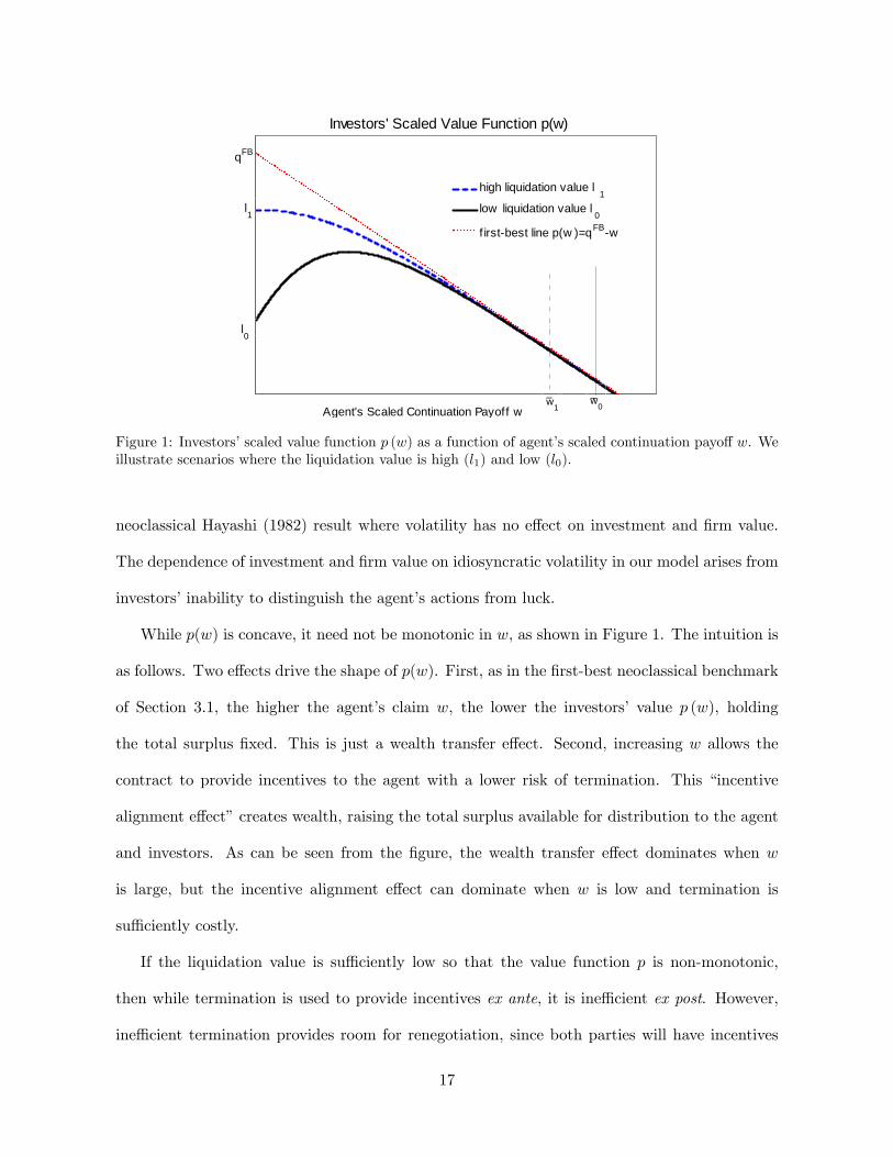
Figure 1: Investors�scaled value function p (w) as a function of agent�s scaled continuation payo¤ w. Weillustrate scenarios where the liquidation value is high (l1) and low (l0).

neoclassical Hayashi (1982) result where volatility has no e¤ect on investment and �rm value.

The dependence of investment and �rm value on idiosyncratic volatility in our model arises from

investors�inability to distinguish the agent�s actions from luck.

While p(w) is concave, it need not be monotonic in w, as shown in Figure 1. The intuition is

as follows. Two e¤ects drive the shape of p(w). First, as in the �rst-best neoclassical benchmark

of Section 3.1, the higher the agent�s claim w, the lower the investors� value p (w), holding

the total surplus �xed. This is just a wealth transfer e¤ect. Second, increasing w allows the

contract to provide incentives to the agent with a lower risk of termination. This �incentive

alignment e¤ect�creates wealth, raising the total surplus available for distribution to the agent

and investors. As can be seen from the �gure, the wealth transfer e¤ect dominates when w

is large, but the incentive alignment e¤ect can dominate when w is low and termination is

su¢ ciently costly.

If the liquidation value is su¢ ciently low so that the value function p is non-monotonic,

then while termination is used to provide incentives ex ante, it is ine¢ cient ex post. However,

ine¢ cient termination provides room for renegotiation, since both parties will have incentives

17

to renegotiate to a Pareto-improving allocation. Thus, with liquidation value l0; the optimal

contract depicted in Figure 1 is not renegotiation-proof (while the contract is renegotiation-proof

with liquidation value l1). In Appendix C, we show that the main qualitative implications of

our model are unchanged when contracts are constrained to be renegotiation-proof. Intuitively,

renegotiation weakens incentives and has the same e¤ect as increasing the agent�s outside option

(which reduces the investors�payo¤).

Alternatively, if the agent can be �red and costlessly replaced, so that the liquidation value

is endogenously determined as in Eq. (22) with � = 0, then p0(0) = 0 and the optimal contract

will be renegotiation-proof. We can also interpret the case with l1 in Figure 1 in this way.

4.2 Average and Marginal q

Now we use the properties of p(w) to derive implications for q. Total �rm value, including the

claim held by the agent, is P (K;W ) +W . Therefore, average q, de�ned as the ratio between

�rm value and capital stock, is denoted by qa and given by10

qa (w) =P (K;W ) +W

K= p (w) + w. (23)

Marginal q measures the incremental impact of a unit of capital on �rm value. We denote

marginal q as qm and calculate it as:

qm (w) =@ (P (K;W ) +W )

@K= PK(K;W ) = p(w)� wp0(w). (24)

While average q is often used in empirical studies due to the simplicity of its measurement,

marginal q determines the �rm�s investment via the standard Euler equations.

One of the most important and well-known results in Hayashi (1982) is that marginal q

equals average q when the �rm�s production and investment technologies exhibit homogeneity

as shown in our neoclassical benchmark case. While our model also features these homogeneity

10Note that excluding the agent�s future compensation w in the de�nition of q does not give the prediction thatTobin�s q equals marginal q even in the neoclassical benchmark (Hayashi (1982)) setting (see Section 3.1). Thus,empirical measures of q that ignore managers�claims may be misspeci�ed.

18

properties, agency costs cause the marginal value of investing, qm, to di¤er from the average

value of capital stock, qa. In particular, comparing (7), (23) and (24) and using the fact that

p0(w) � �1, we have the following inequality:

qFB > qa (w) � qm (w) : (25)

The �rst inequality follows by comparing (21) and the calculation of qFB in (7). Average q

is above marginal q because, for a given level of W , an increase in capital stock K lowers the

agent�s scaled continuation payo¤ w, which lowers the agent�s e¤ective claim on the �rm, and

hence induces a more severe agency problem. The wedge between average and marginal q is

non-monotonic. Average and marginal q are equal when w = 0 and the contract is terminated.

Then qa > qm for w > 0 until the cash payment region is reached, w = w. At that point, the

incentive bene�ts of w are outweighed by the agent�s impatience, so that p0(w) = �1 and again

qa = qm.

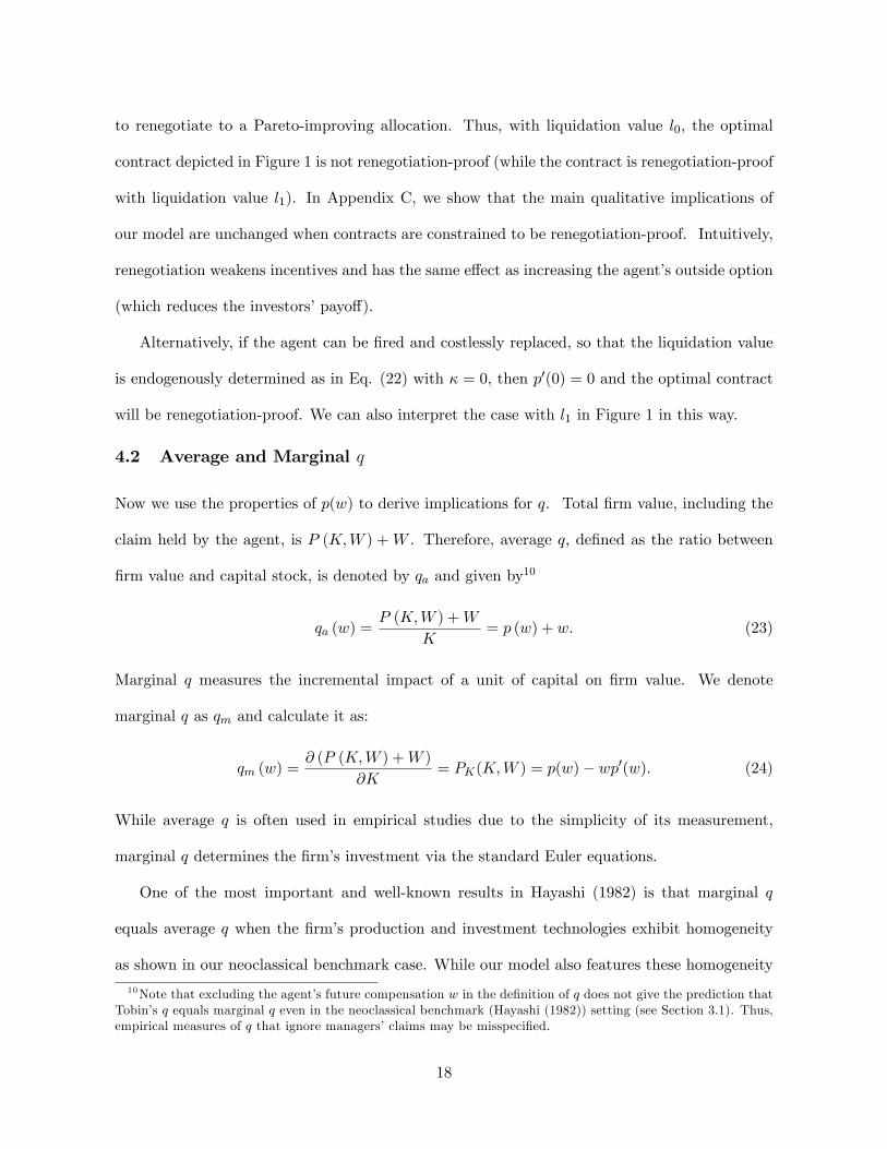
Both average q and marginal q are functions of the agent�s scaled continuation payo¤ w.

Because p0(w) � �1, average q is increasing in w (re�ecting the incentive alignment e¤ect noted

earlier). In addition, the concavity of p(w) implies that marginal q is also increasing in w. In

Figure 2, we plot qa, qm, and the �rst-best average (also marginal) qFB.

It is well understood that marginal and average q are forward looking measures and capture

future investment opportunities. In the presence of agency costs, it is also the case that both

marginal and average q are positively related to the �rm�s pro�t history. Recall that the value

of the agent�s claim w evolves according to (17), and so is increasing with the past pro�ts of the

�rm, and that both marginal and average q increase with w for incentive reasons. Unlike the

neoclassical setting in which q is independent of the �rm�s history, both marginal and average q

in our setting are history dependent.

19

Graphical illustration of qa and q

m

Agent's Scaled Continuation Pay of f w

Average q a versus Marginal q m

Average qa

Marginal qm

firstbest q

w_

qa

qa=qm=l

qa=q

m

qm

p(w)

Agent's Scaled Continuation Pay of f w

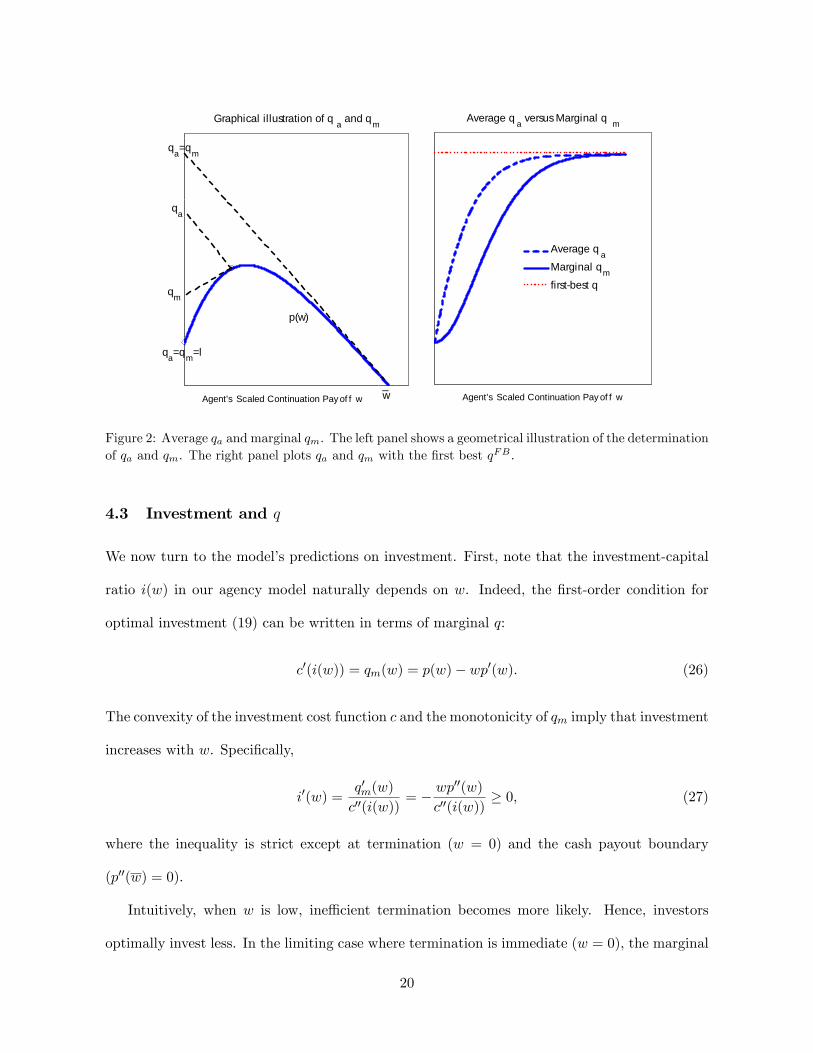
Figure 2: Average qa and marginal qm. The left panel shows a geometrical illustration of the determinationof qa and qm. The right panel plots qa and qm with the �rst best qFB .

4.3 Investment and q

We now turn to the model�s predictions on investment. First, note that the investment-capital

ratio i(w) in our agency model naturally depends on w. Indeed, the �rst-order condition for

optimal investment (19) can be written in terms of marginal q:

c0(i(w)) = qm(w) = p(w)� wp0(w): (26)

The convexity of the investment cost function c and the monotonicity of qm imply that investment

increases with w. Speci�cally,

i0(w) =q0m(w)

c00(i(w))= � wp00(w)

c00(i(w))� 0; (27)

where the inequality is strict except at termination (w = 0) and the cash payout boundary

(p00(w) = 0).

Intuitively, when w is low, ine¢ cient termination becomes more likely. Hence, investors

optimally invest less. In the limiting case where termination is immediate (w = 0), the marginal

20

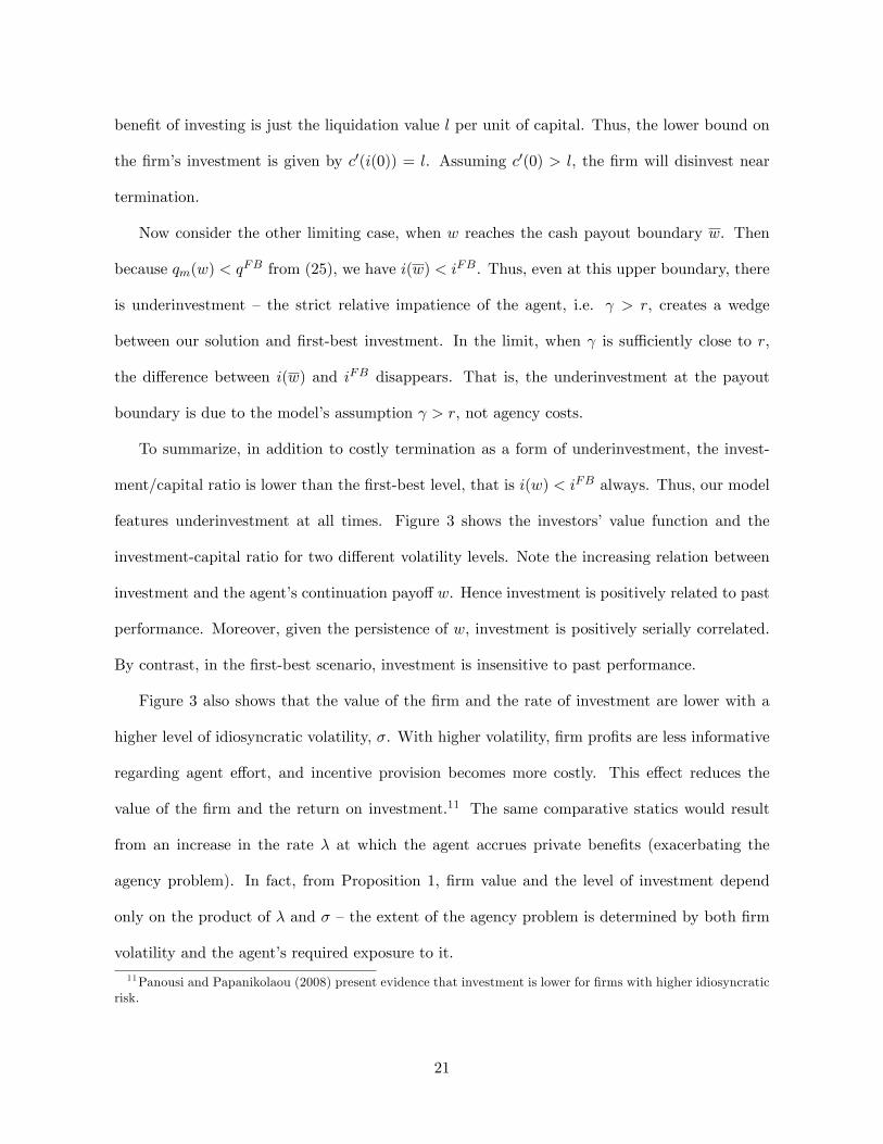
bene�t of investing is just the liquidation value l per unit of capital. Thus, the lower bound on

the �rm�s investment is given by c0(i(0)) = l. Assuming c0(0) > l, the �rm will disinvest near

termination.

Now consider the other limiting case, when w reaches the cash payout boundary w. Then

because qm(w) < qFB from (25), we have i(w) < iFB. Thus, even at this upper boundary, there

is underinvestment � the strict relative impatience of the agent, i.e. > r, creates a wedge

between our solution and �rst-best investment. In the limit, when is su¢ ciently close to r,

the di¤erence between i(w) and iFB disappears. That is, the underinvestment at the payout

boundary is due to the model�s assumption > r, not agency costs.

To summarize, in addition to costly termination as a form of underinvestment, the invest-

ment/capital ratio is lower than the �rst-best level, that is i(w) < iFB always. Thus, our model

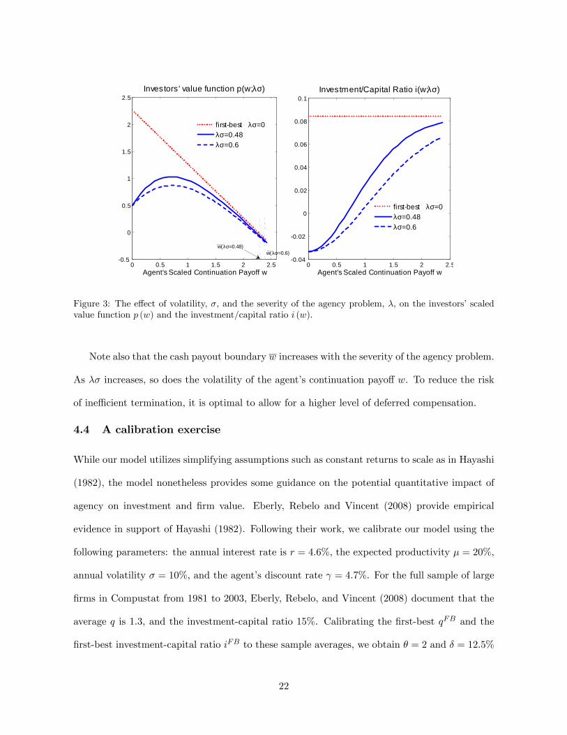
features underinvestment at all times. Figure 3 shows the investors� value function and the

investment-capital ratio for two di¤erent volatility levels. Note the increasing relation between

investment and the agent�s continuation payo¤w. Hence investment is positively related to past

performance. Moreover, given the persistence of w, investment is positively serially correlated.

By contrast, in the �rst-best scenario, investment is insensitive to past performance.

Figure 3 also shows that the value of the �rm and the rate of investment are lower with a

higher level of idiosyncratic volatility, �. With higher volatility, �rm pro�ts are less informative

regarding agent e¤ort, and incentive provision becomes more costly. This e¤ect reduces the

value of the �rm and the return on investment.11 The same comparative statics would result

from an increase in the rate � at which the agent accrues private bene�ts (exacerbating the

agency problem). In fact, from Proposition 1, �rm value and the level of investment depend

only on the product of � and � �the extent of the agency problem is determined by both �rm

volatility and the agent�s required exposure to it.

11Panousi and Papanikolaou (2008) present evidence that investment is lower for �rms with higher idiosyncraticrisk.

21

0 0.5 1 1.5 2 2.50.5

0

0.5

1

1.5

2

2.5


Investors' value function p(w;λσ)

firstbest λσ=0λσ=0.48λσ=0.6

0 0.5 1 1.5 2 2.50.04

0.02

0

0.02

0.04

0.06

0.08

0.1


Investment/Capital Ratio i(w;λσ)

firstbest λσ=0λσ=0.48λσ=0.6

w(λσ=0.48)w(λσ=0.6)

Figure 3: The e¤ect of volatility, �, and the severity of the agency problem, �, on the investors�scaledvalue function p (w) and the investment/capital ratio i (w).

Note also that the cash payout boundary w increases with the severity of the agency problem.

As �� increases, so does the volatility of the agent�s continuation payo¤ w. To reduce the risk

of ine¢ cient termination, it is optimal to allow for a higher level of deferred compensation.

4.4 A calibration exercise

While our model utilizes simplifying assumptions such as constant returns to scale as in Hayashi

(1982), the model nonetheless provides some guidance on the potential quantitative impact of

agency on investment and �rm value. Eberly, Rebelo and Vincent (2008) provide empirical

evidence in support of Hayashi (1982). Following their work, we calibrate our model using the

following parameters: the annual interest rate is r = 4:6%, the expected productivity � = 20%,

annual volatility � = 10%, and the agent�s discount rate = 4:7%. For the full sample of large

�rms in Compustat from 1981 to 2003, Eberly, Rebelo, and Vincent (2008) document that the

average q is 1:3, and the investment-capital ratio 15%. Calibrating the �rst-best qFB and the

�rst-best investment-capital ratio iFB to these sample averages, we obtain � = 2 and � = 12:5%

22

for our model. We choose per unit capital liquidation value l = 0:9 (Henessy and Whited (2005))

and � = 0:75 as baseline parameters.

We then simulate our model at monthly frequency, generating a sample path with 200 years.

We compute the sample average of q and investment-capital ratio i(w). We then repeat the

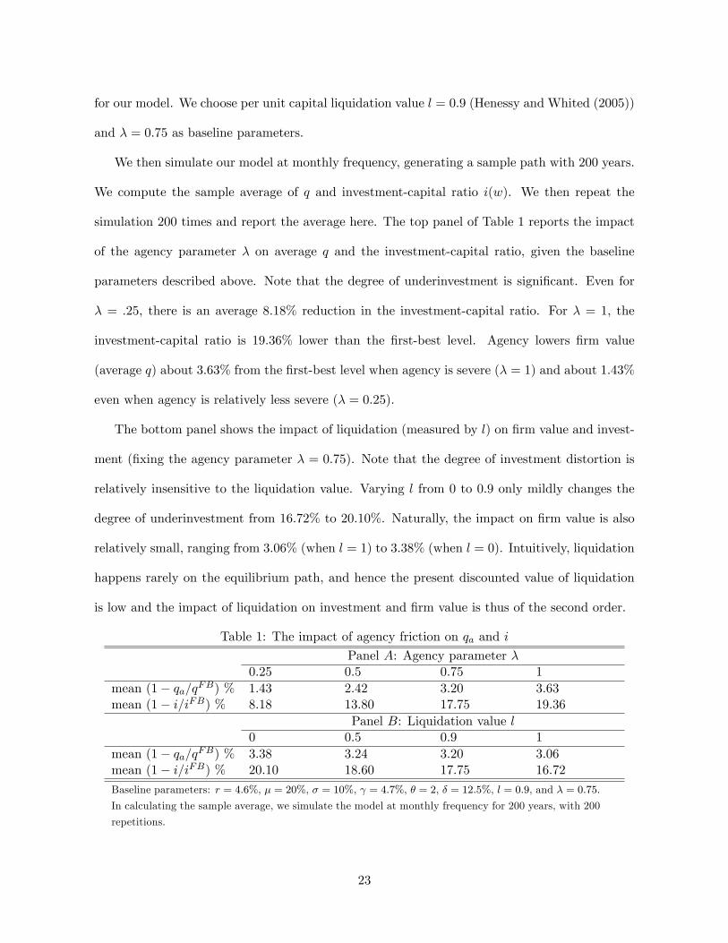
simulation 200 times and report the average here. The top panel of Table 1 reports the impact

of the agency parameter � on average q and the investment-capital ratio, given the baseline

parameters described above. Note that the degree of underinvestment is signi�cant. Even for

� = :25, there is an average 8:18% reduction in the investment-capital ratio. For � = 1, the

investment-capital ratio is 19:36% lower than the �rst-best level. Agency lowers �rm value

(average q) about 3:63% from the �rst-best level when agency is severe (� = 1) and about 1:43%

even when agency is relatively less severe (� = 0:25).

The bottom panel shows the impact of liquidation (measured by l) on �rm value and invest-

ment (�xing the agency parameter � = 0:75). Note that the degree of investment distortion is

relatively insensitive to the liquidation value. Varying l from 0 to 0:9 only mildly changes the

degree of underinvestment from 16:72% to 20:10%. Naturally, the impact on �rm value is also

relatively small, ranging from 3:06% (when l = 1) to 3:38% (when l = 0). Intuitively, liquidation

happens rarely on the equilibrium path, and hence the present discounted value of liquidation

is low and the impact of liquidation on investment and �rm value is thus of the second order.

Table 1: The impact of agency friction on qa and i

Panel A: Agency parameter �0.25 0.5 0.75 1

mean (1� qa=qFB) % 1.43 2.42 3.20 3.63mean (1� i=iFB) % 8.18 13.80 17.75 19.36

Panel B: Liquidation value l0 0.5 0.9 1

mean (1� qa=qFB) % 3.38 3.24 3.20 3.06mean (1� i=iFB) % 20.10 18.60 17.75 16.72

Baseline parameters: r = 4:6%, � = 20%, � = 10%, = 4:7%, � = 2, � = 12:5%, l = 0:9, and � = 0:75.

In calculating the sample average, we simulate the model at monthly frequency for 200 years, with 200

repetitions.

23

5 Implementing the Optimal Contract

In Section 3, we characterized the optimal contract in terms of an optimal mechanism. In this

section, we consider implications of the optimal mechanism for the �rm�s �nancial slack, and

explore the link between �nancial slack and investment.

Recall that the dynamics of the optimal contract are determined by the evolution of the

agent�s continuation payo¤ wt. Because termination occurs when wt = 0, we can interpret wt

as a measure of the �rm�s �distance� to termination. Indeed, from (17), the largest short-run

shock dAt to the �rm�s cash �ows that can occur without termination is given by wt=�. This

suggests that we can interpret mt = wt=� as the �rm�s available �nancial slack, i.e. the largest

short-run loss the �rm can sustain before the agent is terminated and a change of control occurs.

We can formalize this idea in a variety of ways. Financial slack may correspond to the �rm�s

cash reserves (as in Biais et al. (2007)), or a line of credit (as in DeMarzo and Sannikov (2006)

and DeMarzo and Fishman (2007b)), or be a combination of the �rm�s cash and available credit.

Payments to investors may correspond to payouts on debt, equity, or other securities. Rather

than attempt to describe all possibilities, we�ll describe one simple way to implement the optimal

contract, and then discuss which of its features are robust.

Speci�cally, suppose the �rm meets its short-term �nancing needs by maintaining a cash

reserve. (Recall that the �rm will potentially generate operating losses, and so needs access to

cash or credit to operate.) Let Mt denote the level of cash reserves at date t. These reserves

earn interest rate r, and once they are exhausted, the �rm cannot operate and the contract is

terminated.

The �rm is �nanced with equity. Equity holders require a minimum payout rate of12

dDt = [Kt (�� c(it))� ( � r)Mt] dt:

12 If dDt < 0 we interpret this as the maximum rate that the �rm can raise new capital, e.g, by issuing equity.We can show, however, that if � = 1; then dDt > 0.

24

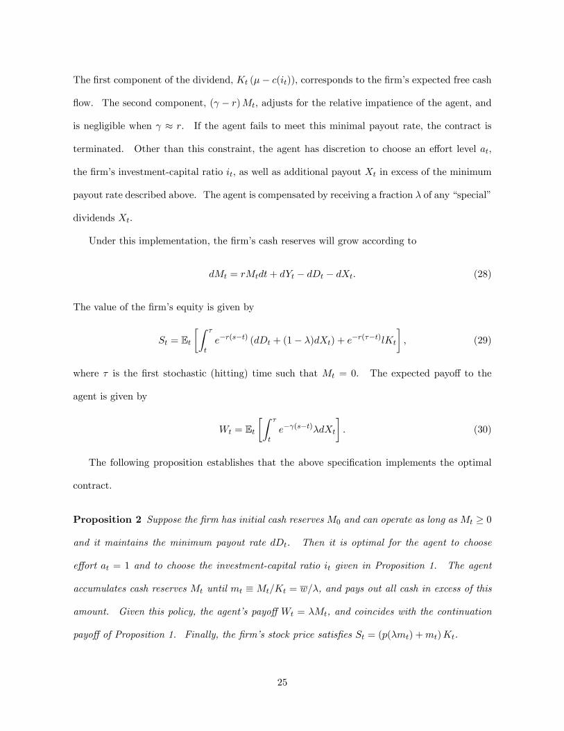
The �rst component of the dividend, Kt (�� c(it)), corresponds to the �rm�s expected free cash

�ow. The second component, ( � r)Mt, adjusts for the relative impatience of the agent, and

is negligible when � r. If the agent fails to meet this minimal payout rate, the contract is

terminated. Other than this constraint, the agent has discretion to choose an e¤ort level at,

the �rm�s investment-capital ratio it, as well as additional payout Xt in excess of the minimum

payout rate described above. The agent is compensated by receiving a fraction � of any �special�

dividends Xt.

Under this implementation, the �rm�s cash reserves will grow according to

dMt = rMtdt+ dYt � dDt � dXt: (28)

The value of the �rm�s equity is given by

St = Et�Z �

te�r(s�t) (dDt + (1� �)dXt) + e�r(��t)lKt

�; (29)

where � is the �rst stochastic (hitting) time such that Mt = 0. The expected payo¤ to the

agent is given by

Wt = Et�Z �

te� (s�t)�dXt

�: (30)

The following proposition establishes that the above speci�cation implements the optimal

contract.

Proposition 2 Suppose the �rm has initial cash reserves M0 and can operate as long as Mt � 0

and it maintains the minimum payout rate dDt. Then it is optimal for the agent to choose

e¤ort at = 1 and to choose the investment-capital ratio it given in Proposition 1. The agent

accumulates cash reserves Mt until mt � Mt=Kt = w=�, and pays out all cash in excess of this

amount. Given this policy, the agent�s payo¤ Wt = �Mt, and coincides with the continuation

payo¤ of Proposition 1. Finally, the �rm�s stock price satis�es St = (p(�mt) +mt)Kt.

25

In this implementation, regular dividends are relatively �smooth� and approximately cor-

respond to the �rm�s expected rate of free cash �ow. The cash �ow �uctuations induced by

the �rm�s productivity shocks are absorbed by the �rm�s cash reserves until the maximal level

of reserves is achieved or the �rm runs out of cash. Also, because the above �nancial policy

implements the optimal contract, there is no ex ante change to the policy (such as issuance of

alternative securities) that will make shareholders better o¤.13

The above implementation is not unique. For example, the minimum dividend payouts

could be equivalently implemented as required coupon payments on long-term debt or preferred

stock. (In fact, such an implementation may be more natural if termination is interpreted as

liquidating the �rm, as opposed to �ring the manager.) Also, rather than solely use cash reserves,

the �rm may maintain its �nancial slack through a combination of cash and credit. In that

case the measure Mt of �nancial slack will correspond to the �rm�s cash and available credit,

and the contract will terminate once these are exhausted.14 Again, �nancial slack Mt will be

proportional to the manager�s continuation payo¤Wt in the optimal contract. In fact because

Wt is a measure of the �rm�s �distance to termination�in the optimal contract, its relation to

the �rm�s �nancial slack is a robust feature of any implementation.

In our implementation, �nancial slack per unit of capital is given by m = w=�. Therefore,

we can reinterpret some earlier results in terms of this measure of �nancial slack. Speci�cally,

we have the following results:

� Financial slack is positively related to past performance.

� Average q (corresponding to enterprise value plus agent rents) and marginal q increase

with �nancial slack.13 If the optimal contract is not renegotiation-proof, then not surprisingly there may be ex post improvements

available to shareholders. See the appendix for further discussion.14The implementation developed here using cash reserves is similar to that in Biais et. al (2007). In DeMarzo

and Fishman (2007b) and DeMarzo and Sannikov (2006), the �rm�s �nancial slack is in the form of a credit line.With a credit line, the minimum dividend payout rate would be reduced by the interest due on the credit lineand the risk-free interest rate on the �rm�s unused credit.

26

� Investment increases with �nancial slack.

� Expected agent cash compensation (over any time interval) increases with �nancial slack.

� The maximal level of �nancial slack is higher for �rm�s with more volatile cash �ows and

�rms with lower liquidation values.15

The investment literature often focuses on the positive relation between �rms�cash �ow and

investment; see for example, Fazzari, Hubbard, and Petersen (1988), Hubbard (1998) and Stein

(2003). While our results are consistent with this e¤ect, our analysis suggests that �nancial

slack (a stock, rather than �ow measure) has a more direct in�uence on investment. It is also

worth noting that our dynamic agency model does not yield a sharp prediction on the sensitivity

of di=dm with respect to �nancial slack. That is, as shown by Kaplan and Zingales (1997) it is

di¢ cult to sign d2i=dm2 without imposing strong restrictions on the cost of investment. Their

result can be understood in the context of our model from Eq. (27), where it is clear that

i0(w), and therefore di=dm, depends on the convexity of the investment cost function c00. Thus,

d2i=dm2 will depend on the third-order derivatives of the cost function.

6 Persistent Price Shocks

The only shocks in our model thus far are the �rm�s idiosyncratic, temporary productivity

shocks. While these shocks have no e¤ect in the neoclassical setting, they obscure the agent�s

actions to create an agency problem. The optimal incentive contract then implies that these

temporary, idiosyncratic shocks have a persistent impact on the �rm�s investment, growth, and

value.

In this section, we extend the model to allow for persistent observable shocks to the �rm�s

pro�tability. As an example, we consider �uctuations in the price of the �rm�s output. These15Unlike our earlier results, this result for volatility does not extend to the level of private bene�ts �:While the

optimal contract (in terms of payo¤s and net cash �ows) only depends on ��, in this implementation the maximallevel of �nancial slack is given by m = w=�, so that although w increases with �; the maximal level of �nancialslack m will tend to decrease with the level of private bene�ts.

27

price shocks di¤er in two important ways from the �rm�s temporary productivity shocks. First,

it is natural to assume that these price shocks are observable and can be contracted on. Second,

because these price shocks are persistent they will a¤ect the �rm�s optimal rate of investment

even in the neoclassical setting.

Our goal is to explore the interaction of public, persistent shocks with the agency problem

and the consequences for investment, �nancial slack, and managerial compensation. As a

benchmark, if the price shocks were purely transitory, they would have no e¤ect on the �rm�s

investment or the agent�s compensation, with or without an agency problem. Investors would

simply absorb the price shocks, insulating the �rm and the agent. As we will show, however, if

the price shocks are persistent they will a¤ect both the optimal level of investment and the agent�s

compensation, with the latter e¤ect having an additional feedback on the �rm�s investment.

We extend our baseline model with i.i.d. productivity shocks to a setting where output price

is stochastic in Section 6.1. Then, we analyze the interaction e¤ects in Section 6.2. Finally,

in Section 6.3 we examine the relation between investment and �nancial slack controlling for

average q.

6.1 The Model and Solution Method

We extend the basic model by introducing a stochastic price �t for the �rm�s output. To keep

the analysis simple, we model �t as a two-state Markov regime-switching process.16 Speci�cally,

�t 2��L; �H

with 0 < �L < �H . Let �n be the transition intensity out of regime n = L or

H to the other regime. Thus, for example, given a current price of �L at date t, the output

price changes to �H with probability �Ldt in the time interval (t; t + dt): The output price �t

is observable to investors and the agent and is contractible. The �rm�s operating pro�t is then

16Piskorski and Tchistyi (2007) consider a model of mortgage design in which they use a Markov switchingprocess to describe interest rates. They were the �rst to incorporate such a process in a continuous-time contractingmodel, and our analysis follows their approach.

28

given by the following modi�cation of Eq. (3):

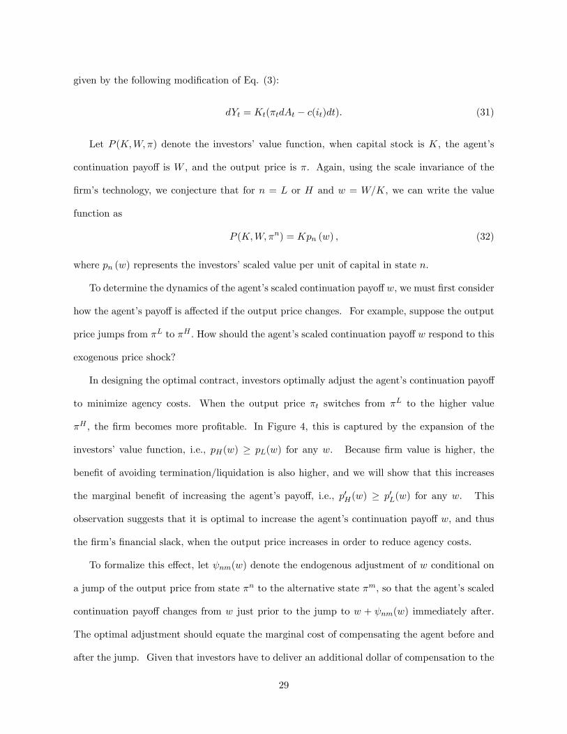
dYt = Kt(�tdAt � c(it)dt). (31)

Let P (K;W; �) denote the investors�value function, when capital stock is K, the agent�s

continuation payo¤ is W , and the output price is �. Again, using the scale invariance of the

�rm�s technology, we conjecture that for n = L or H and w = W=K, we can write the value

function as

P (K;W; �n) = Kpn (w) ; (32)

where pn (w) represents the investors�scaled value per unit of capital in state n.

To determine the dynamics of the agent�s scaled continuation payo¤w; we must �rst consider

how the agent�s payo¤ is a¤ected if the output price changes. For example, suppose the output

price jumps from �L to �H : How should the agent�s scaled continuation payo¤w respond to this

exogenous price shock?

In designing the optimal contract, investors optimally adjust the agent�s continuation payo¤

to minimize agency costs. When the output price �t switches from �L to the higher value

�H , the �rm becomes more pro�table. In Figure 4, this is captured by the expansion of the

investors� value function, i.e., pH(w) � pL(w) for any w. Because �rm value is higher, the

bene�t of avoiding termination/liquidation is also higher, and we will show that this increases

the marginal bene�t of increasing the agent�s payo¤, i.e., p0H(w) � p0L(w) for any w. This

observation suggests that it is optimal to increase the agent�s continuation payo¤ w, and thus

the �rm�s �nancial slack, when the output price increases in order to reduce agency costs.

To formalize this e¤ect, let nm(w) denote the endogenous adjustment of w conditional on

a jump of the output price from state �n to the alternative state �m, so that the agent�s scaled

continuation payo¤ changes from w just prior to the jump to w + nm(w) immediately after.

The optimal adjustment should equate the marginal cost of compensating the agent before and

after the jump. Given that investors have to deliver an additional dollar of compensation to the

29

agent, what is their marginal cost of doing so in each state? The marginal cost is captured by the

marginal impact of w on the investors�value function, i.e., p0n(w). Therefore, the compensation

adjustment nm is given by

p0n(w) = p0m(w + nm(w)) (33)

which is feasible as long as p0n(w) � p0m(0). If p0n(w) > p0m(0), the agent�s payo¤ jumps to zero

( nm(w) = �w) and the contract terminates in order to minimize the di¤erence in the marginal

cost of compensation. See Figure 4; there, if the output price is high and w < wc, where wc is

determined by

p0H(wc) = p0L(0);

a drop in the output price triggers termination.

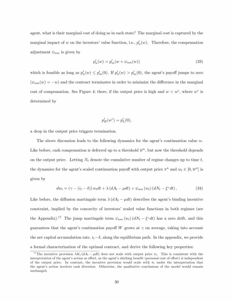
The above discussion leads to the following dynamics for the agent�s continuation value w:

Like before, cash compensation is deferred up to a threshold wn; but now the threshold depends

on the output price. Letting Nt denote the cumulative number of regime changes up to time t,

the dynamics for the agent�s scaled continuation payo¤ with output price �n and wt 2 [0; wn] is

given by

dwt = ( � (it � �))wtdt+ � (dAt � �dt) + nm (wt) (dNt � �ndt) ; (34)

Like before, the di¤usion martingale term � (dAt � �dt) describes the agent�s binding incentive

constraint, implied by the concavity of investors� scaled value functions in both regimes (see

the Appendix).17 The jump martingale term nm (wt) (dNt � �ndt) has a zero drift, and this

guarantees that the agent�s continuation payo¤W grows at on average, taking into account

the net capital accumulation rate, it��, along the equilibrium path. In the appendix, we provide

a formal characterization of the optimal contract, and derive the following key properties:17The incentive provision �Kt (dAt � �dt) does not scale with output price �t. This is consistent with the

interpretation of the agent�s action as e¤ort, as the agent�s shirking bene�t (personal cost of e¤ort) is independentof the output price. In contrast, the incentive provision would scale with �t under the interpretation thatthe agent�s action involves cash diversion. Otherwise, the qualitative conclusions of the model would remainunchanged.

30

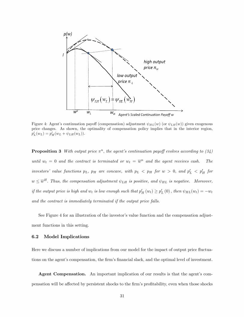
Figure 4: Agent�s continuation payo¤ (compensation) adjustment HL(w) (or LH(w)) given exogenousprice changes. As shown, the optimality of compensation policy implies that in the interior region,p0L(wL) = p0H(wL + LH(wL)).

Proposition 3 With output price �n; the agent�s continuation payo¤ evolves according to (34)

until wt = 0 and the contract is terminated or wt = wn and the agent receives cash. The

investors� value functions pL; pH are concave, with pL < pH for w > 0; and p0L < p0H for

w � wH : Thus, the compensation adjustment LH is positive, and HL is negative. Moreover,

if the output price is high and wt is low enough such that p0H (wt) � p0L (0) ; then HL(wt) = �wt

and the contract is immediately terminated if the output price falls.

See Figure 4 for an illustration of the investor�s value function and the compensation adjust-

ment functions in this setting.

6.2 Model Implications

Here we discuss a number of implications from our model for the impact of output price �uctua-

tions on the agent�s compensation, the �rm�s �nancial slack, and the optimal level of investment.

Agent Compensation. An important implication of our results is that the agent�s com-

pensation will be a¤ected by persistent shocks to the �rm�s pro�tability, even when those shocks

31

are publicly observable and unrelated to the agency problem. Speci�cally, the agent is rewarded

when the output price increases, LH > 0, and is penalized �and possibly immediately termi-

nated �when the output price declines, HL < 0. This result is in contrast with conventional

wisdom that optimal contracts should insulate managers from exogenous shocks and compensate

them based solely on relative performance measures. Rather, in our dynamic model managerial

compensation will optimally be sensitive to the absolute performance of the �rm.

The intuition for this result is that an increase in the �rm�s pro�tability makes it e¢ cient to

reduce the likelihood of termination by increasing the level of the agent�s compensation. Thus,

the optimal contract shifts the agent�s compensation from low price states to high price states.

More generally, in a dynamic agency context, the optimal contract smoothes the marginal cost of

compensation. Unlike static models, in a dynamic setting the marginal cost of compensation is

generally state dependent, as it is cheaper to increase the agent�s rents (and thus align incentives)

in states where the incentive problem is more costly.

We assumed here that the liquidation/termination value of the �rm is independent of the

current output price, thus making termination relatively more costly in the high price state. If

termination corresponds to �ring and replacing the agent, then although lH > lL (�rm value

upon replacement is higher when the output price is high), the qualitative results discussed

above remain unchanged. Indeed, as long as it is costly to replace the agent (� > 0 in (22)),

then wc > 0 and the agent may be �red and replaced if the output price falls.

However, if lH and lL are speci�ed in some alternative manner, it is possible that termination

would be su¢ ciently less costly when the output price were high so that it would be optimal to

reduce the agent�s compensation (and thereby increase the risk of termination) when the output

price increased. But while these speci�c results could change depending on such assumptions,

the more important qualitative result �that the agent�s compensation is a¤ected by persistent

observable shocks �would remain.

32

Hedging and Financial Slack. We can also interpret these results in the context of the

�rm�s �nancial slack. Because LH > 0; it is optimal to increase the �rm�s available slack when

the output price rises, and decrease slack when the output price decreases. This sensitivity could

be implemented, for example, by having the �rm hold a �nancial derivative that pays o¤ when

the output price increases. A similar adjustment to �nancial slack might be implemented with

convertible debt �when the output price and �rm value increases, bondholders convert their

securities, and �nancial slack increases. Whatever the speci�c implementation, it is optimal for

the �rm to increase the sensitivity of its cash position to the output price. Notably, it is not

optimal for the �rm to hedge its output price. Rather, the �rm�s hedging policy should smooth

the changes in the marginal value of �nancial slack.18

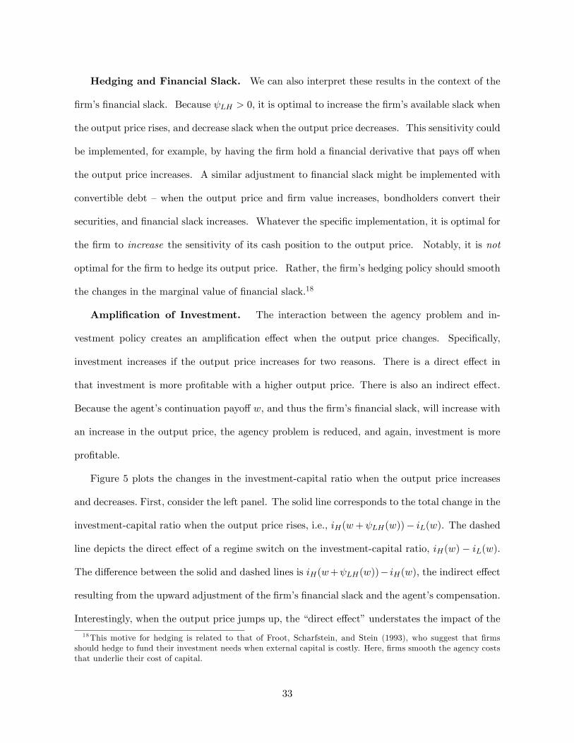
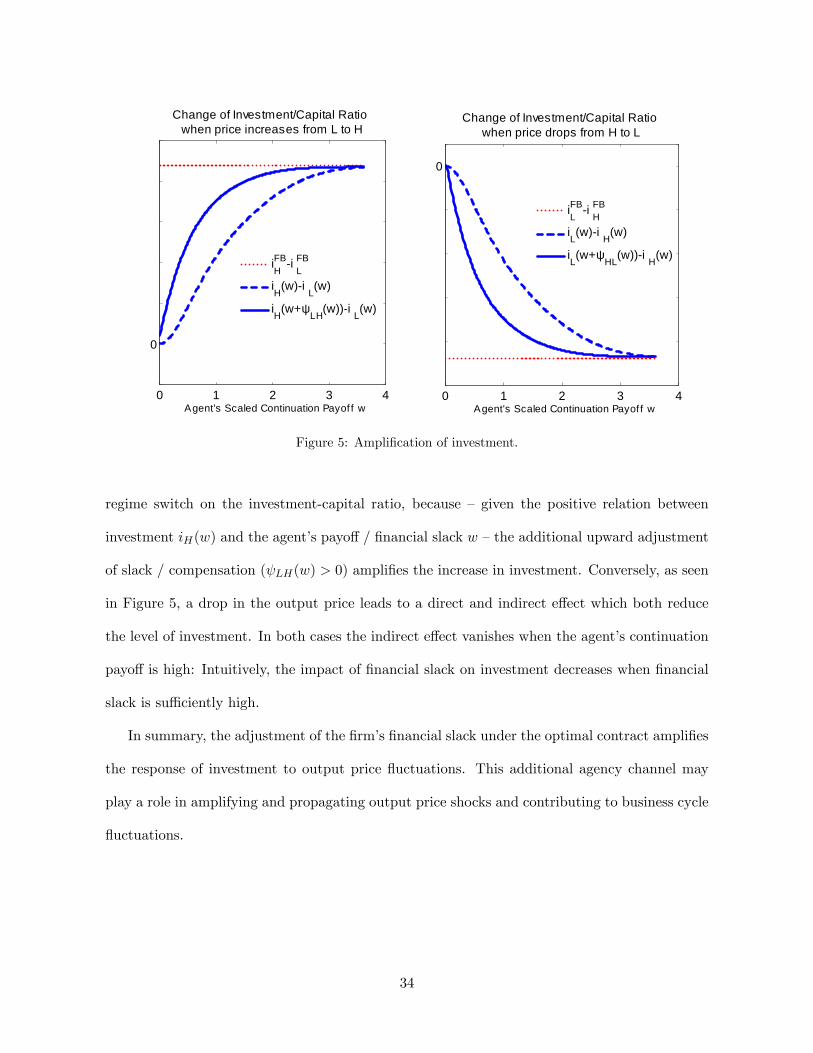
Ampli�cation of Investment. The interaction between the agency problem and in-

vestment policy creates an ampli�cation e¤ect when the output price changes. Speci�cally,

investment increases if the output price increases for two reasons. There is a direct e¤ect in

that investment is more pro�table with a higher output price. There is also an indirect e¤ect.

Because the agent�s continuation payo¤w, and thus the �rm�s �nancial slack, will increase with

an increase in the output price, the agency problem is reduced, and again, investment is more

pro�table.

Figure 5 plots the changes in the investment-capital ratio when the output price increases

and decreases. First, consider the left panel. The solid line corresponds to the total change in the

investment-capital ratio when the output price rises, i.e., iH(w+ LH(w))� iL(w). The dashed

line depicts the direct e¤ect of a regime switch on the investment-capital ratio, iH(w)� iL(w).

The di¤erence between the solid and dashed lines is iH(w+ LH(w))� iH(w); the indirect e¤ect

resulting from the upward adjustment of the �rm�s �nancial slack and the agent�s compensation.

Interestingly, when the output price jumps up, the �direct e¤ect�understates the impact of the

18This motive for hedging is related to that of Froot, Scharfstein, and Stein (1993), who suggest that �rmsshould hedge to fund their investment needs when external capital is costly. Here, �rms smooth the agency coststhat underlie their cost of capital.

33

0 1 2 3 4

0

Agent's Scaled Continuation Payof f w

Change of Investment/Capital Ratiowhen price drops from H to L

iLFBi

HFB

iL(w)i

H(w)

iL(w+ψ

HL(w))i

H(w)

0 1 2 3 4

0

Agent's Scaled Continuation Payof f w

Change of Investment/Capital Ratiowhen price increases from L to H

iHFBi

LFB

iH

(w)iL(w)

iH

(w+ψLH

(w))iL(w)

Figure 5: Ampli�cation of investment.

regime switch on the investment-capital ratio, because � given the positive relation between

investment iH(w) and the agent�s payo¤ / �nancial slack w �the additional upward adjustment

of slack / compensation ( LH(w) > 0) ampli�es the increase in investment. Conversely, as seen

in Figure 5, a drop in the output price leads to a direct and indirect e¤ect which both reduce

the level of investment. In both cases the indirect e¤ect vanishes when the agent�s continuation

payo¤ is high: Intuitively, the impact of �nancial slack on investment decreases when �nancial

slack is su¢ ciently high.

In summary, the adjustment of the �rm�s �nancial slack under the optimal contract ampli�es

the response of investment to output price �uctuations. This additional agency channel may

play a role in amplifying and propagating output price shocks and contributing to business cycle

�uctuations.

34

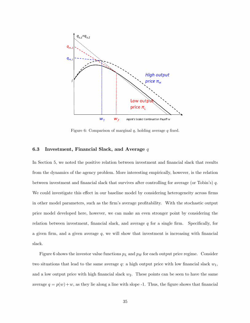
Figure 6: Comparison of marginal q, holding average q �xed.

6.3 Investment, Financial Slack, and Average q

In Section 5, we noted the positive relation between investment and �nancial slack that results

from the dynamics of the agency problem. More interesting empirically, however, is the relation

between investment and �nancial slack that survives after controlling for average (or Tobin�s) q:

We could investigate this e¤ect in our baseline model by considering heterogeneity across �rms

in other model parameters, such as the �rm�s average pro�tability. With the stochastic output

price model developed here, however, we can make an even stronger point by considering the

relation between investment, �nancial slack, and average q for a single �rm. Speci�cally, for

a given �rm, and a given average q, we will show that investment is increasing with �nancial

slack.

Figure 6 shows the investor value functions pL and pH for each output price regime. Consider

two situations that lead to the same average q: a high output price with low �nancial slack w1;

and a low output price with high �nancial slack w2: These points can be seen to have the same

average q = p(w)+w, as they lie along a line with slope -1. Thus, the �gure shows that �nancial

35

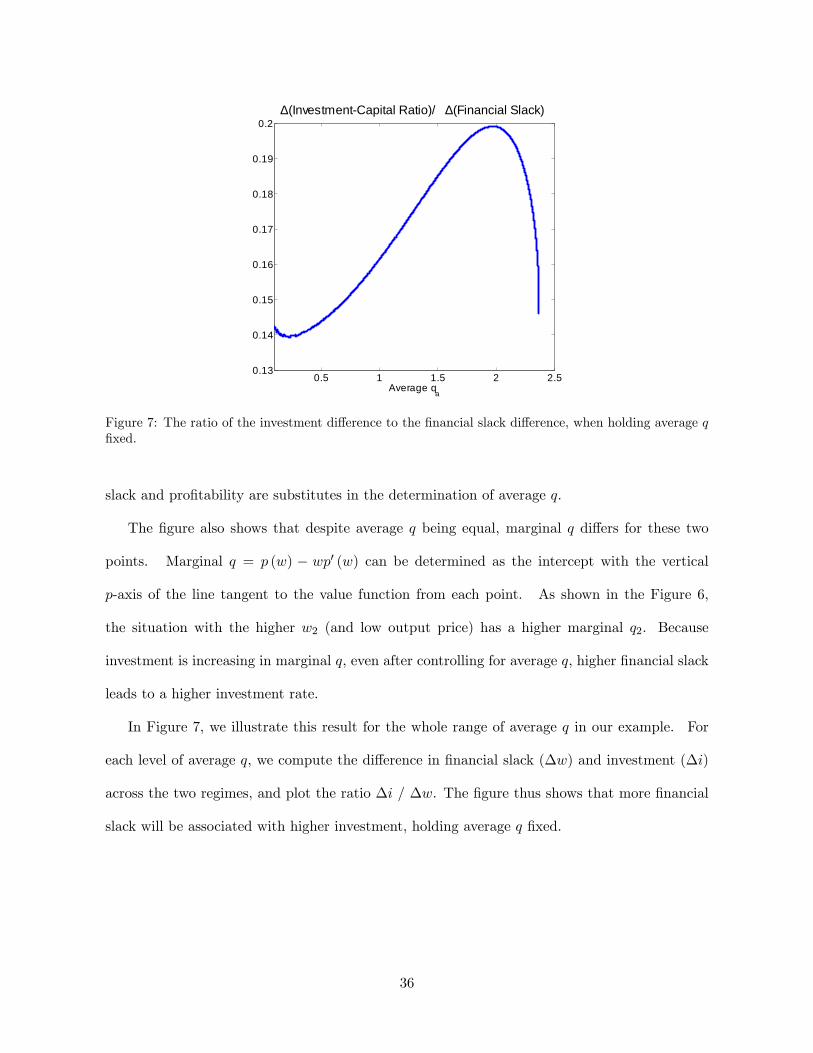
0.5 1 1.5 2 2.50.13

0.14

0.15

0.16

0.17

0.18

0.19

0.2∆(InvestmentCapital Ratio)/ ∆(Financial Slack)

Average qa

Figure 7: The ratio of the investment di¤erence to the �nancial slack di¤erence, when holding average q�xed.

slack and pro�tability are substitutes in the determination of average q:

The �gure also shows that despite average q being equal, marginal q di¤ers for these two

points. Marginal q = p (w) � wp0 (w) can be determined as the intercept with the vertical

p-axis of the line tangent to the value function from each point. As shown in the Figure 6,

the situation with the higher w2 (and low output price) has a higher marginal q2. Because

investment is increasing in marginal q, even after controlling for average q; higher �nancial slack

leads to a higher investment rate.

In Figure 7, we illustrate this result for the whole range of average q in our example. For

each level of average q, we compute the di¤erence in �nancial slack (�w) and investment (�i)

across the two regimes, and plot the ratio �i / �w. The �gure thus shows that more �nancial

slack will be associated with higher investment, holding average q �xed.

36

7 Concluding Remarks

This paper integrates dynamic agency into a neoclassical model of investment. Using a continuous-

time recursive contracting methodology, we characterize the impact of dynamic agency on �rm

value and optimal investment dynamics. Agency costs introduce a history-dependent wedge

between marginal q and average q. Even under the assumptions which imply homogeneity (e.g.

constant returns to scale and quadratic adjustment costs as in Hayashi (1982)), investment is

no longer linearly related to average q. Because of the agency problem, investment is increasing

in past pro�tability. The key state variable in the analysis is the agent�s continuation payo¤.

We show how this state variable can be interpreted as a measure of �nancial slack, allowing us

to relate the results to the �rm�s �nancial slack.

To understand the potential importance of productivity shocks on �rm value and investment

dynamics in the presence of agency con�icts, we extend our model to allow the �rm�s output

price to vary stochastically over time. Here we �nd that investment increases with �nancial slack

after controlling for average q. In addition, the agent�s compensation will depend not only on

the �rm�s realized productivity, but also on realized output prices, even though output prices are

beyond the agent�s control. This result may help to explain the empirical relevance of absolute

performance evaluation. Moreover, this result on compensation also suggests that the agency

problem provides a channel through which the response of investment to output price shocks is

ampli�ed and propagated. A higher output price encourages investment for two reasons. First,

investment becomes more pro�table. Second, the optimal compensation contract rewards the

agent with a higher continuation payo¤, which in turn relaxes the agent�s incentive constraints

and hence further raises investment. In ongoing research, we continue to explore the sensitivity

of managerial compensation to external shocks in a range of dynamic agency contexts.

Our model has a constant returns to scale technology and the wedge between qa and qm

results from the agency problem. Decreasing returns to scale would also lead to qa > qm.

37

Incorporating an agency problem into a model with decreasing returns to scale should lead to

investment dynamics that are similar to those obtained here. A di¤erence, though, is that as

the �rm grows, qm declines and so we would expect investment to be increasing with �nancial

slack but decreasing with �rm size.

38

Appendices

A Proof of Proposition 1

We impose the usual regularity condition on the payment policy

E�Z �

0

e� sdUs

�2<1. (A.1)

And, we require that

E

"Z T

0

�e�rtKt

�2dt

#<1 for all T > 0. (A.2)

and

limT!1

E�e�rTKT

�= 0. (A.3)

Both regularity conditions place certain restrictions on the investment policies. Since the project is

terminated at � , throughout we take the convention that HT1fT>�g = H� for any stochastic process H.

Throughout the proof, we take the adjustment cost c (i) as the commonly used quadratic form.

Lemma 1 For any contract � = fU; �g, there exists a progressively measurable process f�t : 0 � t < �gsuch that the agent�s continuation value Wt evolves according to

dWt = Wtdt� dUt + �tKt (dAt � �dt) (A.4)

under at = 1 all the time. The contract � is incentive-compatible, if and only if �t � � for t 2 [0; �).

In the optimal contract, �t = �, so the above dynamics in (A.4) is the one in (13). The proof is

similar to DeMarzo and Sannikov (2006); we omit the proof here.

Now we verify that the contract and the associated investment policy derived from the Hamilton-

Jacobi-Bellman equation are indeed optimal. The evolution of w = WK follows easily from the evolutions

of W and K. The key ODE (18), under the quadratic adjustment cost and the associated optimal

investment policy, is

(r + �) p(w) = �+(p(w)� wp0(w)� 1)2

2�+ p0(w) ( + �)w +

�2�2

2p00(w): (A.5)

Lemma 2 The scaled investors�value function p(w) is concave on [0; w).

Proof. By di¤erentiating (A.5) we obtain

(r + �) p0 = � (p� wp0 � 1)wp00�

+ ( + �)wp00 + ( + �) p0 +�2�2

2p000. (A.6)

Evaluating (A.6) at the upper-boundary w, and using p0 (w) = �1 and p00 (w) = 0, we �nd

�2�2

2p000(w) = � r > 0;

therefore p00(w � �) < 0. Now let q (w) = p (w)� wp0 (w), and we have

(r + �) q(w) = �+(q(w)� 1)2

2�+ ( � r)wp0 (w) + �2�2

2p00:

39

Suppose that there exists some ew < w such that p00 ( ew) = 0. Choose the largest ew s.t. p00(w + �) < 0.

Evaluating the above equation at ew, we have(r + �) q( ew) = �+

(q( ew)� 1)22�

+ ( � r) ewp0 ( ew) .Since q( ew) < qFB , and (r + �) qFB = � +

(qFB�1)2

2� , we have p0 ( ew) < 0. Therefore evaluating (A.6) at

point ew, we obtain(r + �) p0( ew) = p0( ew) ( + �) + �2�2

2p000( ew),

which implies that p000( ew) = 2(r� )�2�2 p

0( ew) > 0. It is inconsistent with the choice of ew where p00 ( ew) = 0

but p00( ew + �) < 0. Therefore p (�) is strictly concave over the whole domain [0; w). Q.E.D.Take any incentive-compatible contract � = (I; U; �). For any t � � , de�ne its auxiliary gain process

fGg as

Gt (�) =

Z t

0

e�rs (dYs � dUs) + e�rtP (Kt;Wt) (A.7)

=

Z t

0

e�rs�KsdAs � Isds�

�I2s2Ks

� dUs�+ e�rtP (Kt;Wt) ;

where the agent�s continuation payo¤Wt evolves according to (13). Under the optimal contract ��, the

associated optimal continuation payo¤W �t has a volatility ��Kt, and fU�g re�ects W �

t at W�t = wKt.

Recall that wt =Wt=Kt and P (Kt;Wt) = Ktp (wt). Ito�s lemma implies that, for t < � ,

ertdGt = Kt

8>>>>><>>>>>:

264 �rp (wt) + �� It=Kt � �2 (It=Kt)

2+ (It=Kt � �) (p (wt)� wtp0 (wt))

+ wtp0 (wt) +

�2t �2

2 p00 (wt)

375 dt+ [�1� p0 (wt)] dUt=Kt + � [1 + �tp

0 (wt)] dZt

9>>>>>=>>>>>;:

Under the optimal investment policy I�t =Kt and optimal incentive policy �t = �, the �rst piece in

the bracket� which is just our (18)� stays at zero always; and other investment policies and incentives

provision will make this term nonpositive (here we use the concavity of p). The second piece captures

the optimality of the cash payment policy. It is nonpositive since p0 (wt) � �1, but equals zero under theoptimal contract.

Therefore, for the auxiliary gain process we have

dGt (�) = �G (t) dt+ e�rtKt� [1 + �tp

0 (wt)] dZt;

where �G (t) � 0. Let 't � e�rtKt� [1 + �tp0 (wt)]. The condition (A.1) and the condition A.2 imply

that EhR T0'tdZt

i= 0 for 8T > 0 (note that p0 is bounded). And, under � the investors�expected payo¤

is eG (�) � E �Z �

0

e�rsdYs �Z �

0

e�rsdUs + e�r� lK�

�:

40

Then, given any t <1,

eG (�) = E [G� (�)]= E

�Gt^�

�e��+ 1t�� Z �

t

e�rsdYs � e�rsdUs�+ e�r� lK� � e�rtP (Kt;Wt)

�= E

hGt^�

�e��i+ e�rtE��Z �

t

e�r(s�t) (dYs � dUs) + e�r(��t)lK� � P (Kt;Wt)

�1t��

�� G0 +

�qFB � l

�E�e�rtKt

�:

The �rst term of third inequality follows from the negative drift of dGt (�) and martingale property ofR t^�0

'sdZs. The second term is due to the fact that

Et�Z �

t

e�r(s�t) (dYs � dUs) + e�r(��t)lK�

�� qFBKt � wtKt

which is the �rst-best result, and

qFBKt � wtKt � P (Kt;Wt) <�qFB � l

�Kt

as w + p (w) is increasing (p0 � �1). But due to (A.3), we have eG � G0 for all incentive-compatible

contract. On the other hand, under the optimal contract �� the investors�payo¤ eG (��) achieves G0because the above weak inequality holds in equality when t!1.

Finally, we require that the agent�s shirking bene�t � � �� be su¢ ciently small to ensure the

optimality of a = 1 all the time. Similar to DeMarzo and Sannikov (2007) and He (2007), there is a

su¢ cient condition for the optimality of a = f�g against at = 0 for some t. Let bw = argwmax p (w), and

we require that

(p (w)� wp0 (w)� 1)2

2�� (r + �) p (w)� p0 (w) [( + �)w � �] for all w

Since the left side is increasing in w, and right side dominates p�

� +�

�� r

r+�

�p ( bw)� p� �

+�

��(see the

proof in DeMarzo and Sannikov (2006)), a su¢ cient condition is

(p (w) + w � 1)2

2�� p

��

+ �

�� rr + �

�p ( bw)� p� �

+ �

��:

B Proof for Proposition 2

We need to verify that under the proposed scheme, the agent�s value function given the relevant state

(M;K) is V (M;K) = �M , and his optimal policy is the one we obtained in Proposition 1. We take the

�guess and verify�approach. Under the proposed implementation, the evolution of the cash reserve M is

dMt = rMtdt+ dYt � dDt � dXt

= rMtdt+KtdAt �Ktc (it) dt� [Kt�dt�Ktc (it) dt� ( � r)Mtdt]� dXt

= Mtdt+Kt (dAt � �dt)� dXt;

41

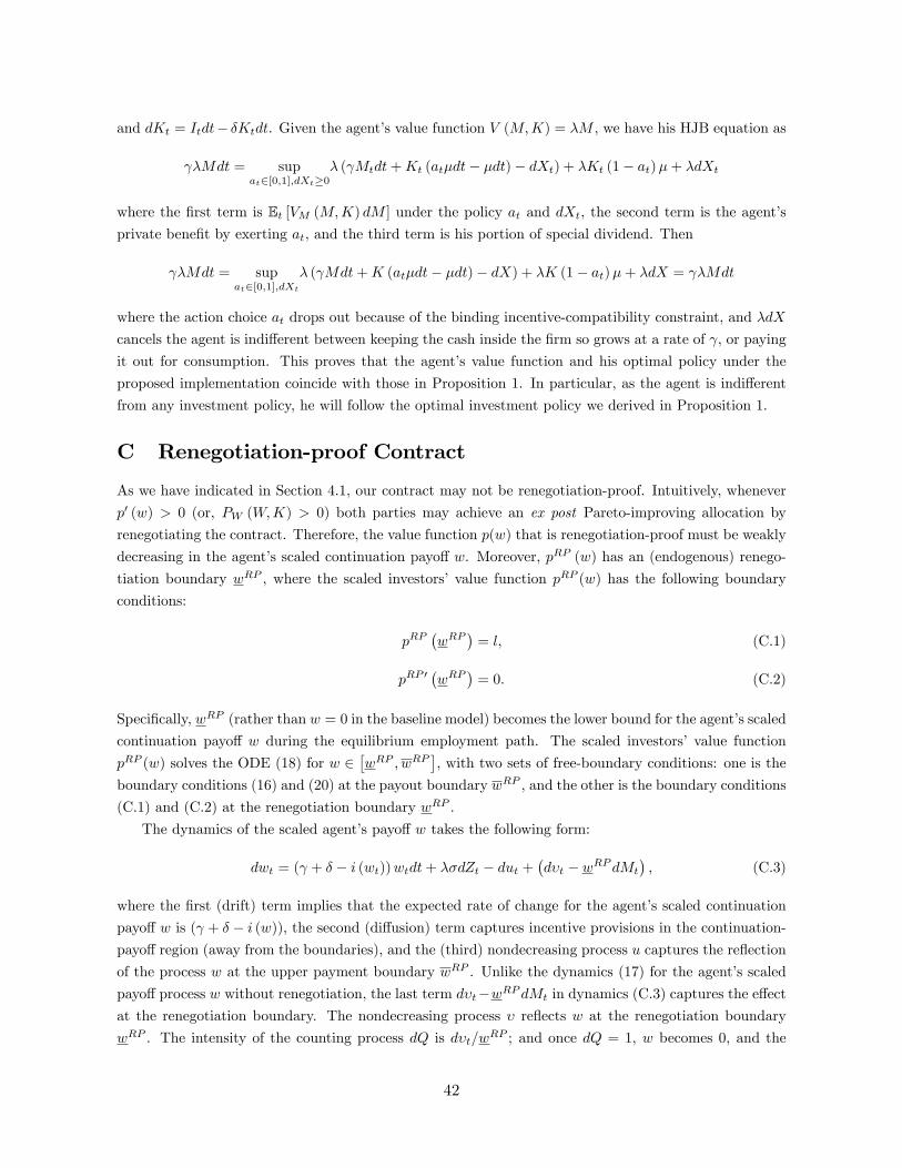
and dKt = Itdt� �Ktdt. Given the agent�s value function V (M;K) = �M , we have his HJB equation as

�Mdt = supat2[0;1];dXt�0

� ( Mtdt+Kt (at�dt� �dt)� dXt) + �Kt (1� at)�+ �dXt

where the �rst term is Et [VM (M;K) dM ] under the policy at and dXt, the second term is the agent�s

private bene�t by exerting at, and the third term is his portion of special dividend. Then

�Mdt = supat2[0;1];dXt

� ( Mdt+K (at�dt� �dt)� dX) + �K (1� at)�+ �dX = �Mdt

where the action choice at drops out because of the binding incentive-compatibility constraint, and �dX

cancels the agent is indi¤erent between keeping the cash inside the �rm so grows at a rate of , or paying

it out for consumption. This proves that the agent�s value function and his optimal policy under the

proposed implementation coincide with those in Proposition 1. In particular, as the agent is indi¤erent

from any investment policy, he will follow the optimal investment policy we derived in Proposition 1.

C Renegotiation-proof Contract

As we have indicated in Section 4.1, our contract may not be renegotiation-proof. Intuitively, whenever

p0 (w) > 0 (or, PW (W;K) > 0) both parties may achieve an ex post Pareto-improving allocation by

renegotiating the contract. Therefore, the value function p(w) that is renegotiation-proof must be weakly

decreasing in the agent�s scaled continuation payo¤ w. Moreover, pRP (w) has an (endogenous) renego-

tiation boundary wRP , where the scaled investors�value function pRP (w) has the following boundary

conditions:

pRP�wRP

�= l; (C.1)

pRP 0�wRP

�= 0: (C.2)

Speci�cally, wRP (rather than w = 0 in the baseline model) becomes the lower bound for the agent�s scaled

continuation payo¤ w during the equilibrium employment path. The scaled investors� value function

pRP (w) solves the ODE (18) for w 2�wRP ; wRP

�, with two sets of free-boundary conditions: one is the

boundary conditions (16) and (20) at the payout boundary wRP , and the other is the boundary conditions

(C.1) and (C.2) at the renegotiation boundary wRP .

The dynamics of the scaled agent�s payo¤ w takes the following form:

dwt = ( + � � i (wt))wtdt+ ��dZt � dut +�d�t � wRP dMt

�; (C.3)

where the �rst (drift) term implies that the expected rate of change for the agent�s scaled continuation

payo¤ w is ( + � � i (w)), the second (di¤usion) term captures incentive provisions in the continuation-

payo¤ region (away from the boundaries), and the (third) nondecreasing process u captures the re�ection

of the process w at the upper payment boundary wRP . Unlike the dynamics (17) for the agent�s scaled

payo¤ process w without renegotiation, the last term d�t�wRP dMt in dynamics (C.3) captures the e¤ect

at the renegotiation boundary. The nondecreasing process � re�ects w at the renegotiation boundary

wRP . The intensity of the counting process dQ is d�t=wRP ; and once dQ = 1, w becomes 0, and the

42

0 0.5 1 1.5 2 2.5 3 3.5 42

1.5

1

0.5

0

0.5

1

1.5

2

2.5


Investors' Scaled Value Function

0 0.5 1 1.5 2 2.5 3 3.5 40.04

0.02

0

0.02

0.04

0.06

0.08

0.1


Investment/Captial Ratio

Firstbest p FB(w)=q FBwp(w)pRP(w) under Rene.proof

Firstbest i FB

i(w)iRP(w) under Rene.proof

wRP w wRP_ _

wRP_ _

Figure 8: Renegotiation proofness. The original scaled value function p (w) is not renegotiation-proof,because p0 (0) > 0. For the renegotiation-proof contract, wRP is the lower bound for the agent�s scaledcontinuation payo¤ w, with the following properties: p

�wRP

�= p (0) = l, and p0

�wRP

�= 0. The value

function pRP (w) solves the ODE (18) subject to the boundary conditions (16)-(20) and the above statedconditions at wRP .

�rm is liquidated.19 Note that the additional term d�t�wRP dQt is a compensated Poisson process, andhence a martingale increment.

We illustrate the contracting behavior at the renegotiation boundary through the following intuitive

way. When the agent�s poor performance drives w down to wRP , the two parties run a lottery. With a

probability of d�t=wRP , the �rm is liquidated. If the �rm is not liquidated, the agent stays at the rene-

gotiation boundary wRP . Here, the stochastic termination is to achieve the �promise-keeping�constraint

so that w is indeed the scaled continuation payo¤ with expected growth rate + � � i (w) as speci�ed inProposition 1. To see this, by running this lottery, the agent could potentially lose

�d�t=w

RP��wRP = dvt,

which just compensates the re�ection gain d�t if the �rm is not liquidated.

Since renegotiation further worsens the agency con�ict, we expect not only a greater value reduction

for investors, but also a stronger underinvestment distortion. Figure 8 shows this result.

19Technically speaking, the counting process has a survival probability Pr (Qt = 0) = exp��t=wRP

�.

43

D Appendix for Section 6

D.1 Characterization of Optimal Contracting with Stochastic Prices

Fix regime L as the current regime (similar results hold for regime H upon necessary relabelling.) Based

on (31) and (34) in Section 6, the following Bellman equation holds for P (K;W; �L):

rP (K;W; �L) = supI,

��LK � I �G(I;K)

�+ (I � �K)PK +

� W �LH(K;W )�L

�PW

+�2�2K2

2PWW + �L

�P (K;W +LH(K;W ); �

H)� P (K;W; �L)�; (D.1)

where the investment I and compensation adjustmentLH(K;W ) (both are unscaled) are state-dependent

controls.

The investment policy I (K;W;n), by taking a FOC condition, is similar to the baseline case. The

�rst-order condition (FOC) for optimal LH(K;W ), given that the solution takes an interior solution,

yields that

PW (K;W; �L) = PW (K;W +LH(K;W ); �

H); (D.2)

As discussed in the main text, the optimal contract equates the marginal cost of delivering compensation,

i.e., �PW , across di¤erent Markov states at any time. However, in general, the solution of nm(K;W )might be binding (corner solution), as the agent�s continuation payo¤ after the regime change has to be

positive. Therefore, along the equilibrium path the optimal nm(K;W ) might bind, i.e., nm(K;W ) +

W � 0 holds with equality.The scale invariance remains: with w =W=K, we let pn(w) = P (K;W; �n)=K, in(w) = I(K;W; �n)=K,

nm (w) = nm(K;W;n)=K, and upper payment boundary wn =W (K;�n)=K. Similar to equation (19),

in(w) =PK(K;W;n)� 1

�=pn(w)� wp0n(w)� 1

�. (D.3)

Combining this result with the above analysis regarding nm (w)�s (notice that PW (K;W; �n) = p0n(w)),

the following proposition characterizes the ODE system fpng when the output price is stochastic.

Proposition 4 For 0 � w � wn (the continuation-payo¤ region for regime n), the scaled investor�s value

function pn (w) and the optimal payment threshold wn solve the following coupled ODEs:

(r + �) pL(w) = ��L +(pL(w)� wp0L(w)� 1)

2

2�+ p0L(w)

�( + �)w � �L LH (w)

�+�2�2

2p00L(w)

+ �L (pH(w + LH (w))� pL(w)) ; 0 � w � wL,

(r + �) pH(w) = ��H +(pH(w)� wp0H(w)� 1)

2

2�+ p0H(w)

�( + �)w � �H HL (w)

�+�2�2

2p00H(w)

+ �H (pL(w + HL (w))� pH(w)) ; 0 � w � wH , (D.4)

subject to the following boundary conditions at the upper boundary wn:

p0n(wn) = �1; (D.5)

p00n(wn) = 0; (D.6)

44

and the left boundary conditions at liquidation:

pn(0) = ln; n = 1; 2:

The scaled endogenous compensation adjustment functions nm (w) satisfy:

p0n(w) = p0m(w + nm (w))

if w + nm (w) > 0 (interior solution); otherwise nm (w) = �w. For w > wn (cash-payment regions),

pn(w) = pn(wn)� (w � wn).Proof. See Section D.2.

In solving the coupled ODEs in Proposition 4 with the optimal payment threshold wn and the

endogenous compensation adjustment functions nm (w), we take the following numerical iteration steps:

1. Solve for p(0)L and p(0)H without price changes (i.e., setting ��s to zero.) This is essentially solving a

nonlinear ODE with a free-boundary condition about w(0)n .

2. Given p(0)L and p(0)H , obtain the compensation adjustment function (0)HL (w) based on Proposition

4.

3. Given (0)HL (w) and p(0)L , calculate p(1)H by solving the high-state one-dimensional nonlinear ODE

(i.e., the second equation) in Eq. (D.4). The resulting solution is p(1)H with the free boundary w(1)H .

4. Obtain (0)LH (w) based on p

(1)H and p

(0)L , and then calculate p(1)L by solving the low-state one-

dimensional nonlinear ODE (i.e., the �rst equation) in (D.4). The resulting solution is p(1)L with

the free boundary w(1)L .

5. Given p(1)L and p(1)H , update (1)HL (w).

6. Then repeat the procedures after step 3, until converge. The convergence is criteria is

max

�supw

�p(j+1)L � p(j)L

�; supw

�p(j+1)H � p(j)H

��< 10�5:

D.2 Proof for Proposition 3

Lemma 3 Both pn�s are strictly concave for 0 � w < wn.

Proof. Denote two states as n;m. By di¤erentiating (D.4) we obtain

(r + �) p0n = �(pn � wp0n � 1)wp00n

�+ p00n � [( + �)w � �n nm (w)] + p0n ( + � � �n 0nm (w)) +

�2�2

2p000n

+ �n (p0m(w + nm (w)) (1 + 0nm (w))� p0n) .

Notice that when nm (w) takes an interior solution, p0m(w+ nm (w)) = p0n(w); and otherwise 0nm (w) =

�1. Either condition implies that

(r + �) p0n = �(pn � wp0n � 1)wp00n

�+ p00n � [( + �)w � �n nm (w)] + p0n ( + �) +

�2�2

2p000n , (D.7)

45

which takes a similar form as in (A.6). Similar to the argument in the proof of Proposition 2 we can

show that p00n(wn � �) < 0 and p00m(wm � �) < 0.Denote �n = ��n. Let qn (w) = pn (w) � wp0n (w), i.e., the marginal q that captures the investment

bene�t. We have

(r + � + �n) qn(w) = �n +(qn(w)� 1)2

2�+ �mqm (w + nm (w)) + ( � r)wp0n (w) +

�2�2

2p00n

(r + � + �m) qm(w + nm (w)) = �m +(qm(w + nm (w))� 1)2

2�+ �nqn (w)

+ ( � r) (w + nm (w)) p0m (w + nm (w)) +�2�2

2p00m (w + nm (w))

(D.8)

Recall that the �rst-best pair�qFBn ; qFBm

�solves the system8><>: (r + � + �n) qFBn = �n +

(qFBn �1)2

2� + �nqFBm

(r + � + �m) qFBm = �m +(qFBm �1)

2

2� + �mqFBn

:

It is understood throughout the proof that as in the Hayashi (1982) with quadratic adjustment cost,

(qn; qm) in Eq. (D.8) and�qFBn ; qFBm

�all take the smaller root in solving the quadratic equations.

Suppose that there exists some points so that pn is convex. Pick the largest ew such that p00n ( ew) = 0but p00n ( ew + ") < 0, and p00n(w) � 0 for w 2 ( ew;wn). If nm ( ew) is interior, then let

k = p0n ( ew) = p0m ( ew + nm ( ew)) ; p00n ( ew) = p00m ( ew + nm ( ew)) (1 + 0nm ( ew)) = 0;Clearly, if p00m ( ew + nm ( ew)) = 0, then

(r + � + �n) qn( ew) = �n +(qn( ew)� 1)2

2�+ �mqm ( ew + nm ( ew)) + ( � r) ewk

(r + � + �m) qm( ew + nm ( ew)) = �m +(qm( ew + nm ( ew))� 1)2

2�+ �nqn ( ew) + ( � r) ( ew + nm ( ew)) k

Since a positive k in the above system will imply that qn > qFBn and qm > qFBm , we must have k < 0.

Then evaluating (A.6) at the point ew, we obtain�2�2

2p000n ( ew) = (r � ) p0n ( ew) = (r � ) k > 0.

This is inconsistent with the choice of ew where p00n ( ew) = 0 but p00n( ew + ") < 0. Notice that the above

argument applies to the case p00m ( ew + nm ( ew)) > 0.Now we consider the case 1+ 0nm ( ew) = 0 but p00m (w + nm (w)) < 0. We must have p0n ( ew) > 0 and

p000n ( ew) < 0 according to the above argument. In the neighborhood of ew �nd two points ew�� < ew < ew+��where �; � are positive, such that p00n ( ew � �) > p00n ( ew) = 0 > p00n ( ew + ��), but ( ew � �) p0n ( ew � �) =( ew + ��) p0n ( ew + ��) = k > 0. Therefore,

(r + � + �n) qn( ew � �) = �n +(qn( ew � �)� 1)2

2�+ �nqm ( ew � �+ nm ( ew � �)) + ( � r) k + �2�2

2p00n ( ew � �)

(r + � + �n) qn( ew + ��) = �n +(qn( ew + ��)� 1)2

2�+ �nqm ( ew + ��+ nm ( ew + ��)) + ( � r) k + �2�2

2p00n ( ew + ��)

46

Because 1 + 0nm ( ew) = 0, the di¤erence in qm will be dominated (since it is in a lower order) by the

di¤erence in p00n�s. Now since p00n ( ew � �) > p00n ( ew + ��), it implies that qn( ew��) > qn( ew+��). But because

qn( ew��)�qn( ew+��) = pn ( ew � �)�pn( ew+��) < 0 according to ( ew � �) p0n ( ew � �) = ( ew + ��) p0n ( ew + ��),contradiction.

Finally consider the case where nm ( ew) is binding at �w. Take the same approach; notice that inthis case the points after regime switching are exactly 0. Therefore the same argument applies, and pn (�)is strictly concave over the whole domain [0; wn). Q.E.D.

Once the concavity of pn�s is established, the veri�cation argument is similar to the baseline case in

Appendix A.

Now we show the properties of compensation adjustment functions. For simplicity take �n = �m = �.

We focus on HL (w). Once HL (w) < 0 is shown, it immediately follows that LH (w) > 0.

Because pH (w) > pL (w) while pL (0) = pH (0) = l, we know p0H (0) > p0L (0), and HL (w) = �wwhen w is small. Then the claim that HL (w) = �w for w lower than a threshold wc such that

p0H (wc) = p0L (0) follows from the concavity of both p�s. From then on, we focus on the area where the

jump functions take interior solutions.

Consider �q (w) = qH (w) � qL (w + HL (w)), which is the di¤erence between marginal q�s across

the two points before and after jump. It starts at zero (both q = l), and must be positive in the payment

boundary, as eventually qL = pL (w) + w < pH (w) + w = qH . Notice that

�q0 (w) = �wp00H (w) + (w + HL (w)) (1 + 0HL (w)) p00L (w + HL (w)) ;

and the slope becomes zero on the upper boundary wH . Focus on w�s that are below the payment region.

When takes interior solutions, p0H (w) = p0L (w + HL (w)), and p00H (w) = p00L (w + HL (w)) (1 +

0HL (w)) :

Therefore �q0 (w) = p00H (w) HL (w), and HL (w) = 0 if and only if �q0 (w) = 0. Moreover, �q (w) is

decreasing if and only if HL (w) is positive.

The following lemma shows that HL (wH) = wL � wH � 0 on the upper payment boundary; lateron we will show HL (wH) < 0 strictly.

Lemma 4 The upper payment boundary wH � wL so that HL (wH) = wL � wH � 0.

Proof. We prove by contradiction. Suppose that HL (wH) = wL �wH > 0. According to (D.8), at

the upper boundary, we have (r + � + �) qn = �n +(qn�1)2

2� + �qm � ( � r)wn, therefore

(r + � + 2�) (qH � qL) = �H � �L +(qH � qL) (qH + qL + 2)

2�+ ( � r) (wL � wH) : (D.9)

Moreover, HL (wH) > 0 implies that �q (w) is decreasing for w < wH around its vicinity. Take bw,which is the largest w such that HL ( bw) = 0 and �q0 ( bw) = 0. (The existence of such bw follows from

the fact HL (0+) < 0.) This implies that �q ( bw) reaches its local maximum and �q ( bw) > qH � qL;

and 0HL ( bw) � 0. However, denoting qL( bw) = bqL and qH( bw) = bqH , (D.8) implies that (r + � + �) bqn =�n +

(bqn�1)22� + �bqm + ( � r) bwp0n ( bw) + �2�2

2 p00n ( bw), which says that(r + � + 2�)�q ( bw) = �H � �L +

�q ( bw) (bqL + bqH + 2)2�

+�2�2

2[p00H ( bw)� p00L ( bw)] : (D.10)

Comparing to (D.9), since bqL + bqH < qL + qH as q is increasing with w, in order for �q ( bw) > qH � qL

we must have the last term in (D.10) to be strictly positive, or p00H ( bw) > p00L ( bw). But recall that

p00H ( bw) = p00L ( bw) (1 + 0HL ( bw)); concavity of pn�s and 0HL ( bw) � 0 yields a contradiction.47

Now we proceed to show that HL (w) � 0 always. Since HL (wH) � 0 and HL (0+) < 0, for

any w such that HL (w) > 0, we always can �nd two points bw < ew closest to w such that HL ( bw) = HL ( ew) = 0, �q0 ( bw) = �q0 ( ew) = 0, �q ( bw) > �q ( ew), and 0HL ( bw) > 0, 0HL ( ew) < 0. We have

(r + � + 2�)�q ( bw) = �H � �L +�q ( bw) (bqL + bqH + 2)

2�+�2�2

2p00L ( bw) 0HL ( bw)

< �H � �L +�q ( bw) (bqL + bqH + 2)

2�

and (r + � + 2�)�q ( ew) = �H ��L+ �q( ew)(eqL+eqH+2)2� + �2�2

2 p00L ( ew) 0HL ( ew) > �H ��L+ �q( ew)(eqL+eqH+2)2� .

Finally, because bqL + bqH < eqL + eqH , �q ( bw) < �q ( ew), contradiction.A similar argument rules out the case that there 9 bw, s.t. HL ( bw) = 0HL ( bw) = 0, while HL (w) � 0

for all w. Suppose not, then �q0 ( bw) = 0, and(r + � + 2�)�q ( bw) = �H � �L +

�q ( bw) (bqL + bqH + 2)2�

:

For w = bw+ �, after neglecting some terms with an order higher than �2 (note that HL ( bw + �) is in theorder of �2)

(r + � + 2�)�q ( bw + �) = �H � �L +�q ( bw + �) (qL ( bw + �) + bqH ( bw + �) + 2)

2�

+ ( � r) HL ( bw + �) p0H ( bw + �) + �2�2

2p00L ( bw + �) 0HL ( bw + �)

The �rst term in the second line is in a lower order than �, as HL ( bw) = 0HL ( bw) = 0. The second termin fact is positive. Because qL ( bw + �) + bqH ( bw + �)� (bqL + bqH) is in the order of �, this contradicts with�q0 ( bw) = 0.

Finally we rule out the case of wH = wL so HL (w) = 0. At w, we have 0HL (w) = 0. It is because

p000H (w) = p000L (w) (1 + 0HL (w)), and p

000L (w) = p000H (w) =

2( �r)�2�2 . Now consider the point w � �:

(r + � + 2�)�q (w � �) = �H � �L +�q (w � �) (qL (w � �) + qH (w � �) + 2)

2�+

( � r) HL (w � �) p0H (w � �) +�2�2

2p00L (w � �) 0HL (w � �) :

One can show that, compared to the value at w, qL (w � �) + qH (w � �) is �2 order smaller. Again, the�rst term in the second line is in lower order, and the second term is negative. Therefore, �q (w � �)should be in �2 order smaller. However,

�q00 (w) = p000H (w) HL (w) + p00H (w)

0HL (w) = 0;

contradiction. Q.E.D.

48

References

[1] Abel, A. B., and J. C. Eberly, 1994, �A Uni�ed Model of Investment Under Uncertainty�, American

Economic Review 84, 1369-1384.

[2] Abel, A. B., and J. C. Eberly, 2005, �Investment, Valuation, and Growth Options�, Working paper,

Wharton School, University of Pennsylvania, and Kellogg School of Management, Northwestern

University.

[3] Albuquerque, R., and H. Hopenhayn, 2004, �Optimal Lending Contracts and Firm Dynamics�,

Review of Economic Studies 71, 285-315.

[4] Atkeson, A., 1991, International Lending with Moral Hazard and Risk of Repudiation, Econometrica

59, 1069�1089.

[5] Biais, B., T. Mariotti, G. Plantin, and J. Rochet, 2007, �Dynamic Security Design: Convergence to

Continuous Time and Asset Pricing Implications�, Review of Economic Studies 74, 345-390.

[6] Bolton, P., and D. Scharfstein, 1990, �A Theory of Predation Based on Agency Problems in Financial

Contracting �, American Economic Review 80, 93-106.

[7] Caballero, R., 1999, �Aggregate Investment�, in J. B. Taylor, and M. Woodford (eds.) Handbook of

Macroeconomics (North Holland: Amsterdam), 813-62.

[8] Clementi, G. L., and H. A. Hopenhayn, 2006, �A Theory of Financing Constraints and Firm Dy-

namics�, Quarterly Journal of Economics 121, 229�265.

[9] Cooper, R. and J. Ejarque, 2003, Financial Frictions and Investment: Requiem in q, Review of

Economic Dynamics 6, 710-28.

[10] Cooper, R. and J. Haltiwanger, 2006, �On the Nature of Capital Adjustment Costs�, Review of

Economic Studies 73, 3, 611-633

[11] DeMarzo, P. and M. Fishman, 2007a, �Agency and Optimal Investment Dynamics�, Review of

Financial Studies 20, 151-188.

[12] DeMarzo, P. and M. Fishman, 2007b, �Optimal Long-Term Financial Contracting�, Review of Fi-

nancial Studies 20, 2079-2128.

[13] DeMarzo, P. and Y. Sannikov, 2006, �A Continuous-Time Agency Model of Optimal Contracting

and Capital Structure�, Journal of Finance 61, 2681-2724.

[14] Diamond, D. W., 1984, �Financial Intermediation and Delegated Monitoring�, Review of Economic

Studies 51, 393�414.

[15] Dixit, A.,1993, The Art of Smooth Pasting, Vol. 55 in Fundamentals of Pure and Applied Economics,

Harwood Academic Publishers.

49

[16] Eberly, J. C., S. Rebelo, and N. Vincent, 2008, �Investment and Value: A Neoclassical Benchmark�,

Working Paper, Northwestern University.

[17] Fazzari, S., G. Hubbard, and B. Petersen, 1988, �Financing constraints and corporate investment,�

Brooking Papers on Economic Activity 1, 141-195.

[18] Froot, K. A., D. Scharfstein, and J. Stein, 1993, �Risk Management: Coordinating Corporate In-

vestment and Financing Policies�, Journal of Finance 48, 1629-1658.

[19] Green, E., 1987, �Lending and the Smoothing of Uninsurable Income�, in E. Prescott and N. Wallace

(eds.) Contractual Arrangements for Intertemporal Trade. Minneapolis: University of Minnesota

Press.

[20] Gomes, J. F., 2001, Financing Investment, American Economic Review 91, 1263-85.

[21] Gromb, D., 1999, �Renegotiation in Debt Contracts�, Working Paper, MIT.

[22] Hayashi, F., 1982, �Tobin�s q, and Average q: A Neoclassical interpretation�, Econometrica 50,

215-224.

[23] He, Z., 2007, �Optimal Executive Compensation when Firm Size Follows Geometric Brownian Mo-

tion�, forthcoming in Review of Financial Studies.

[24] Hennessy, C. A., and T. M. Whited, 2006, �How Costly is External Financing? Evidence from a

Structural Estimation�, Journal of Finance 62, 1705-1745.

[25] Hubbard, G., 1998, �Capital Markets Imperfections and Investment�, Journal of Economic Litera-

ture 36, 193-225.

[26] Kaplan, S. and L. Zingales, 1997, �Do Investment-Cash Flow Sensitivities Provide Useful Measure

of Finance Constraints?�, Quarterly Journal of Economics 112, 169-215.

[27] Ljungqvist, L. and T. J. Sargent, 2004, Recursive Macroeconomic Theory, Cambridge Massachusetts:

MIT Press.

[28] Lorenzoni, G., and K. Walentin, 2007, �Financial Frictions, Investment and Tobin�s q�, Working

Paper, MIT.

[29] Panousi, V., and D. Papanikolaou, 2008, �Investment, Idiosyncratic Risk, and Ownership�, Working

Paper, Northwestern University.

[30] Phelan, C., and R. Townsend, 1991, �Computing Multi-period, Information Constrained Optima�,

Review of Economic Studies 58, 853�881.

[31] Philippon, T., and Y. Sannikov, 2007, Real Options in a Dynamic Agency Model, with Applications

to Financial Development, IPOs, and Business risk, Working Paper, NYU Stern School.

[32] Piskorski, T., and A. Tchistyi, 2007, �Optimal Mortgage Design�, Working paper, Columbia Uni-

versity and NYU.

50

[33] Quadrini, V., 2004, �Investment and Liquidation in Renegotiation-Proof Contracts with Moral Haz-

ard�, Journal of Monetary Economics 51, 713-751.

[34] Sannikov, Y., 2006, �Agency Problems, Screening, and Increasing Credit Lines�, Working Paper,

UC Berkeley.

[35] Schmid, L., 2008, �A Quantitative Dynamic Agency Model of Financing Constraints�, Working

Paper, Duke University.

[36] Spear, S. and S. Srivastava, 1987, �On Repeated Moral Hazard with Discounting,�Review of Eco-

nomic Studies 54, 599-607.

[37] Stein, J., 2003, �Agency, Investment and Corporate Investment,� in G. Constantinides, M. Harris,

and R. Stulz (eds.) Handbook of the Economics of Finance (North Holland: Amsterdam)

[38] Tchistyi, A., 2005, �Security Design with Correlated Hidden Cash Flows: The Optimality of Perfor-

mance Pricing�, Working paper, NYU.

51

Documents

Dynamic Agency and the q Theory of Investment