Embed Size (px)
Citation preview

Defence Research andDevelopment Canada
Recherche et developpementpour la defense Canada
CAN UNCLASSIFIED
Dwell Time Minimization for UnambiguousRadar Range and Doppler Measurements
Alexander Michael DanielDRDC – Ottawa Research Centre
Defence Research and Development CanadaScientific ReportDRDC-RDDC-2019-R006July 2019
CAN UNCLASSIFIED

CAN UNCLASSIFIED
IMPORTANT INFORMATIVE STATEMENTS
This document was reviewed for Controlled Goods by DRDC using the Schedule to the Defence Production Act.
Disclaimer: This publication was prepared by Defence Research and Development Canada an agency of the Department ofNational Defence. The information contained in this publication has been derived and determined through best practice andadherence to the highest standards of responsible conduct of scientific research. This information is intended for the use of theDepartment of National Defence, the Canadian Armed Forces (“Canada") and Public Safety partners and, as permitted, may beshared with academia, industry, Canada’s allies, and the public (“Third Parties"). Any use by, or any reliance on or decisionsmade based on this publication by Third Parties, are done at their own risk and responsibility. Canada does not assume anyliability for any damages or losses which may arise from any use of, or reliance on, the publication.
Endorsement statement: This publication has been peer-reviewed and published by the Editorial Office of Defence Research andDevelopment Canada, an agency of the Department of National Defence of Canada. Inquiries can be sent to:[email protected].
c© Her Majesty the Queen in Right of Canada, Department of National Defence, 2019
c© Sa Majesté la Reine en droit du Canada, Ministère de la Défense nationale, 2019
CAN UNCLASSIFIED
Abstract
With the advent of modern phased-array radar systems, the classic problem of disambiguat-ing radar range and velocity measurements can be recast in the context of radar resourcemanagement as being a problem about achieving some desired unambiguous range andvelocity while using a minimal amount of time. This paper develops a method for unam-biguous range and velocity extension that combines features of traditional multiple-pulse-repetition-frequency and waveform-diverse approaches in order to mitigate their respectiveshortcomings. This scheme is paired with an optimization framework that minimizes thetotal dwell time subject to constraints fixing minimum detection performance. Analysis ofthe optimization problem reveals a hidden convexity that forms the basis of a branch-and-bound solution, which is evaluated numerically to generate insight into the relationshipbetween the parameters and performance of the system. Simulation is then used both tovalidate the scheme generally and to identify some practical shortcomings. Future researchdirections are identified to mitigate these shortcomings and to make the scheme a plausiblecandidate for real-time use in a practical radar resource management framework, includingthe use of more sophisticated waveforms, the development of a real-time solution heuristic,and the incorporation of clutter into the system model.
Significance for defence and security
This paper is ultimately about minimizing the time it takes to detect high-speed targets,while extending the ranges at which these targets can be detected. When hostile inboundtargets are detected at greater distances than they would otherwise normally be, more timeis available to deploy adequate countermeasures.
DRDC-RDDC-2019-R006 i
Résumé
L’arrivée des radars à éléments en phase a permis de redéfinir le problème classique de ladésambiguïsation des mesures radar de distance et de vélocité ; dans le contexte de la gestiondes ressources radar, ce problème devient comment déterminer la distance et la vélocité avecune précision adéquate dans un délai le plus court possible. Le présent document décrit uneméthode de mesure non ambigüe de la portée et de la vélocité qui combine certains aspectsdes méthodes habituelles (fréquences de répétition d’impulsions multiples et formes d’ondediverses) qui vise à atténuer leurs inconvénients respectifs. Cette démarche hybride estdoublée d’un cadre d’optimisation qui minimise le temps de calcul total en fonction decontraintes, ce qui établit un rendement de détection minimal. Une analyse du problèmed’optimisation a révélé une convexité qui a formé la base d’une solution de séparation etd’évaluation, solution évaluée numériquement afin de mieux comprendre les liens entre lesparamètres et le rendement du système. Des simulations ont ensuite servi tant à validerle principe général qu’à identifier certaines lacunes en pratique. Le document relève desavenues de recherche possibles afin de combler ces lacunes et créer un candidat plausiblepour des applications en temps réel dans un cadre pratique de gestion des ressources radar,notamment l’utilisation de formes d’ondes plus avancées, le développement d’un algorithmeheuristique de recherche d’une solution en temps réel, et l’intégration du fouillis dans lemodèle du système.
Importance pour la défense et la sécurité
En gros, le document traite de la minimisation du temps consacré à la détection des ciblesse déplaçant à grande vitesse tout en élargissant la portée de détection de ces mêmes cibles.Détecter l’approche de cibles hostiles à partir d’une plus grande distance qu’on le peutnormalement laisserait plus de temps pour déployer des contre-mesures adéquates.
ii DRDC-RDDC-2019-R006
Table of contents
Abstract . . . . . . . . . . . . . . . . . . . . . . . . . . . . . . . . . . . . . . . . . . . i
Significance for defence and security . . . . . . . . . . . . . . . . . . . . . . . . . . . i
Résumé . . . . . . . . . . . . . . . . . . . . . . . . . . . . . . . . . . . . . . . . . . . ii
Importance pour la défense et la sécurité . . . . . . . . . . . . . . . . . . . . . . . . ii
Table of contents . . . . . . . . . . . . . . . . . . . . . . . . . . . . . . . . . . . . . . iii
List of figures . . . . . . . . . . . . . . . . . . . . . . . . . . . . . . . . . . . . . . . . iv
List of tables . . . . . . . . . . . . . . . . . . . . . . . . . . . . . . . . . . . . . . . . v
Acknowledgements . . . . . . . . . . . . . . . . . . . . . . . . . . . . . . . . . . . . . vi
1 Introduction . . . . . . . . . . . . . . . . . . . . . . . . . . . . . . . . . . . . . . . 1
1.1 Background . . . . . . . . . . . . . . . . . . . . . . . . . . . . . . . . . . . 1
1.2 Previous Work . . . . . . . . . . . . . . . . . . . . . . . . . . . . . . . . . . 2
1.2.1 Multiple Pulse Repetition Frequency Approaches . . . . . . . . . . 2
1.2.2 Waveform Diversity Approaches . . . . . . . . . . . . . . . . . . . 5
1.3 Paper Contribution and Organization . . . . . . . . . . . . . . . . . . . . . 7
2 Problem Formulation . . . . . . . . . . . . . . . . . . . . . . . . . . . . . . . . . . 8
2.1 System Model . . . . . . . . . . . . . . . . . . . . . . . . . . . . . . . . . . 8
2.2 Disambiguation Scheme . . . . . . . . . . . . . . . . . . . . . . . . . . . . . 9
2.3 Performance Considerations . . . . . . . . . . . . . . . . . . . . . . . . . . 10
2.3.1 Dwell Time . . . . . . . . . . . . . . . . . . . . . . . . . . . . . . . 12
2.3.2 Computer Clock Considerations . . . . . . . . . . . . . . . . . . . 12
2.3.3 Bandwidth Limitations . . . . . . . . . . . . . . . . . . . . . . . . 13
2.3.4 Radar Visibility . . . . . . . . . . . . . . . . . . . . . . . . . . . . 14
2.3.5 Maximum Duty Cycle . . . . . . . . . . . . . . . . . . . . . . . . . 16
DRDC-RDDC-2019-R006 iii

2.3.6 Target Detection . . . . . . . . . . . . . . . . . . . . . . . . . . . . 17
2.3.7 Velocity Decodability . . . . . . . . . . . . . . . . . . . . . . . . . 21
2.3.8 Range Migration . . . . . . . . . . . . . . . . . . . . . . . . . . . . 21
2.4 Inner Problem Statement . . . . . . . . . . . . . . . . . . . . . . . . . . . . 22
3 Problem Analysis . . . . . . . . . . . . . . . . . . . . . . . . . . . . . . . . . . . . 22
3.1 A Convex Subproblem . . . . . . . . . . . . . . . . . . . . . . . . . . . . . 22
3.2 A Second Convex Subproblem . . . . . . . . . . . . . . . . . . . . . . . . . 25
3.3 A Heuristic Solution Algorithm . . . . . . . . . . . . . . . . . . . . . . . . 28
4 Towards Practical Implementation . . . . . . . . . . . . . . . . . . . . . . . . . . 30
4.1 Chaotic Phase Codes . . . . . . . . . . . . . . . . . . . . . . . . . . . . . . 31
4.2 A Hybrid Detector . . . . . . . . . . . . . . . . . . . . . . . . . . . . . . . 33
4.3 Frequency Compensation . . . . . . . . . . . . . . . . . . . . . . . . . . . . 37
4.4 Clustering Algorithm . . . . . . . . . . . . . . . . . . . . . . . . . . . . . . 39
5 Numerical Evaluation and Simulation . . . . . . . . . . . . . . . . . . . . . . . . 40
5.1 Optimization Problem Solution . . . . . . . . . . . . . . . . . . . . . . . . 40
5.2 System Simulation . . . . . . . . . . . . . . . . . . . . . . . . . . . . . . . 46
6 Discussion . . . . . . . . . . . . . . . . . . . . . . . . . . . . . . . . . . . . . . . . 54
6.1 Additional Optimization Constraints . . . . . . . . . . . . . . . . . . . . . 56
6.2 Real-Time Solution of the Optimization Problem . . . . . . . . . . . . . . 58
6.3 Masking and Other Waveform Considerations . . . . . . . . . . . . . . . . 60
6.4 Clutter . . . . . . . . . . . . . . . . . . . . . . . . . . . . . . . . . . . . . . 63
6.5 Other Practical Considerations . . . . . . . . . . . . . . . . . . . . . . . . . 63
7 Summary . . . . . . . . . . . . . . . . . . . . . . . . . . . . . . . . . . . . . . . . 65
References . . . . . . . . . . . . . . . . . . . . . . . . . . . . . . . . . . . . . . . . . . 68
Annex A: Computation of Frequency Compensation-Induced Artefacts . . . . . . . 76
iv DRDC-RDDC-2019-R006
List of figures
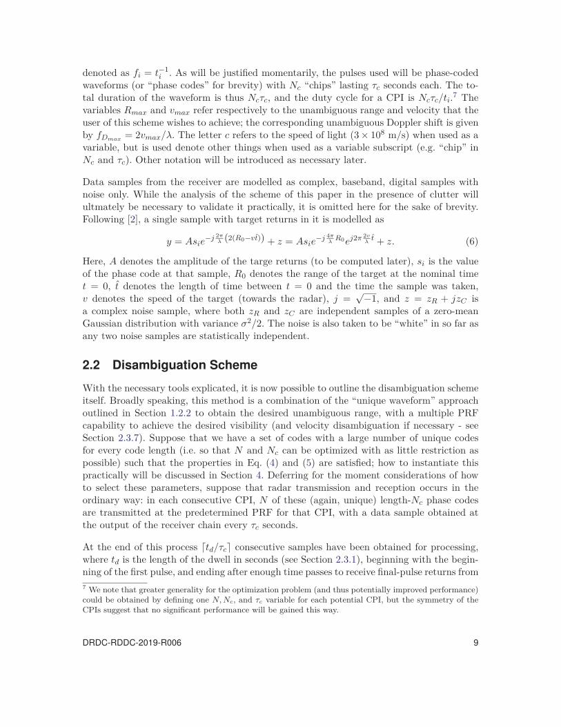
Figure 1: A visual representation of time in the final CPI of the scheme. Forconvenience, tM and 2Rmax/c are assumed to be multiples of Ncτc. . . . 13
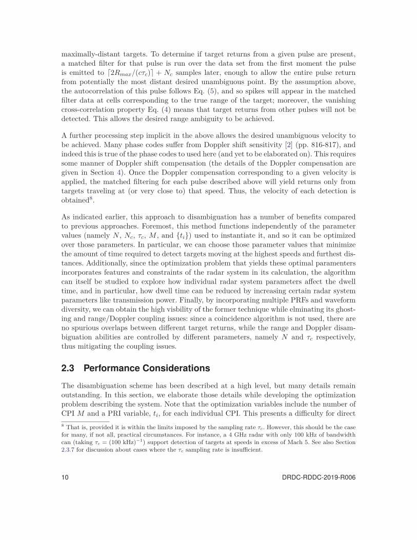
Figure 2: The per-pulse, per-CPI visibility for a system with M = 3, N = 20,Nc = 10, {t1, t2, t3} = {70τc, 75τc, 80τc}, and Rmax = 500cτc/2. Rowscorrespond to individual pulse visibility and columns correspond torange cells, while black cells are eclipsed and white cells are not. . . . . 15
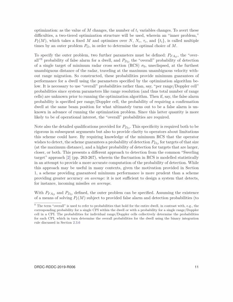
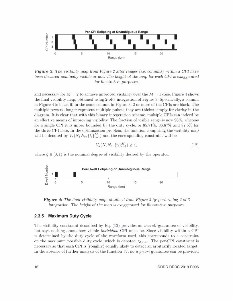
Figure 3: The visibility map from Figure 2 after ranges (i.e. columns) within aCPI have been declared nominally visible or not. The height of the mapfor each CPI is exaggerated for illustrative purposes. . . . . . . . . . . . 16
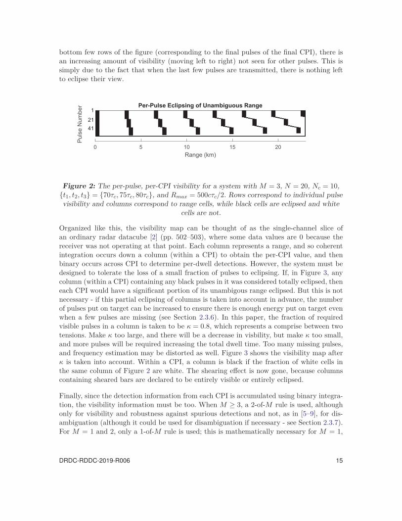
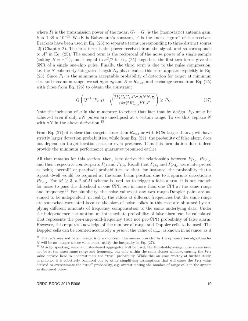
Figure 4: The final visibility map, obtained from Figure 3 by performing 2-of-3integration. The height of the map is exaggerated for illustrative purposes. 16
Figure 5: The dwell time of the system as a function of the nominal visibilityparameter ζ. . . . . . . . . . . . . . . . . . . . . . . . . . . . . . . . . . 42
Figure 6: The dwell time of the system as a function of the radar quality, whichhere is varied by varying the transmission power Pt. . . . . . . . . . . . 43
Figure 7: The dwell time of the system as a function of the available bandwidth. . 44
Figure 8: The dwell time of the system as a function of the maximum duty cycleof the radar. . . . . . . . . . . . . . . . . . . . . . . . . . . . . . . . . . . 46
Figure 9: The range response with thresholds for a maximally-distant, fast, andminimally-sized target. The range resolution is 9 m. . . . . . . . . . . . 47
Figure 10: The frequency response in cell 2557 of CPI 1 with thresholds for amaximally-distant, fast, and minimally-sized target. . . . . . . . . . . . 49
Figure 11: The frequency response in cell 2557 of CPI 2 with thresholds for amaximally-distant, fast, and minimally-sized target. . . . . . . . . . . . 49
Figure 12: The frequency response in cell 2557 of CPI 3 with thresholds for amaximally-distant, fast, and minimally-sized target. . . . . . . . . . . . 50
Figure 13: The range response with thresholds for a close target. The rangeresolution is 9 m. . . . . . . . . . . . . . . . . . . . . . . . . . . . . . . . 51
Figure 14: A magnified view of Figure 13 showing how some sidelobes pass the NPthreshold. . . . . . . . . . . . . . . . . . . . . . . . . . . . . . . . . . . . 51
DRDC-RDDC-2019-R006 v
Figure 15: The frequency response in cell 426 of CPI 1 with thresholds for a closetarget. . . . . . . . . . . . . . . . . . . . . . . . . . . . . . . . . . . . . . 52
Figure 16: The frequency response in cell 426 of CPI 3 with thresholds for a closetarget. . . . . . . . . . . . . . . . . . . . . . . . . . . . . . . . . . . . . . 52
Figure 17: The detector response to cross-correlations for a target at 3824 m. . . . 53
Figure 18: The detector response to cross-correlations for a target at 8927 m. . . . 54
Figure 19: A spurious sidelobe detection from a target at 6371 m. The rangeresolution is 9 m, so this false detection appears to be due to a target at10 km, but the absence of similar detections in other CPI prevents thealgorithm from making this decision. . . . . . . . . . . . . . . . . . . . . 55
Figure 20: A comparison of the naive bound (Eq. (1)) and a bound for theproposed scheme (Eq. (63)) for M = 3 at 3 GHz and for the defaultparameters of Table 1. . . . . . . . . . . . . . . . . . . . . . . . . . . . . 67
Figure A.1: A typical frequency-domain response for the first CPI, withN = 129, Nc = 20, τc = 6 · 10−8, and t1 = 200τc. . . . . . . . . . . . . . 77
Figure A.2: A typical frequency-domain response for the second CPI, withN = 129, Nc = 20, τc = 6 · 10−8, and t2 = 203τc. . . . . . . . . . . . . . 78
vi DRDC-RDDC-2019-R006

List of tables
Table 1: Default System Parameters. . . . . . . . . . . . . . . . . . . . . . . . . . 41
Table 2: The Almost-Linear Relationship Between Radar Quality and Dwell Time. 43
Table 3: Energy-on-Target Variation with Bandwidth. . . . . . . . . . . . . . . . 44
Table 4: Optimal Values for Default System Parameters. . . . . . . . . . . . . . . 47
DRDC-RDDC-2019-R006 vii

Acknowledgements
The author would like to thank Peter Moo for his guidance and support thoughout theprocess of conducting this research.
viii DRDC-RDDC-2019-R006
1 Introduction1.1 Background
Ambiguity in range and velocity measurement is a fundamental problem for pulse-Dopplerradar systems. Consider a pulse-Doppler radar operating at a fixed p ulse r epetition fre-quency (PRF), illuminating a target with multiple identical pulses. If the target is so faraway that the reflection o f o ne p ulse d oes n ot r eturn t o t he r adar b efore t he n ext pulseis transmitted,1 the receiver cannot determine which receptions are due to which pulses,and so cannot unambiguously determine the return time of a pulse, rendering unambiguousrange estimation of a target impossible. Radar operators wishing to extend the range atwhich targets can be unambiguously detected (henceforth, the “unambiguous range”) musttherefore reduce the PRF of the radar. Conversely, each pulse provides a sample of theDoppler shift induced by the target’s motion, and so by the Nyquist sampling theorem [1],the fixed PRF causes aliasing of all frequencies greater than half its value in magnitude, andconsequently prevents unambiguous estimation of target velocity. Radar operators wishingto extend the maximum unambiguous velocity of the radar system must therefore
the PRF of the radar.
These two basic desiderata are in direct opposition; it is straightforward to show [2] that forthe system described above to have a maximum unambiguous range Rmax and a maximumunambiguous velocity vmax (i.e. can detect objects moving radially toward or away fromthe radar at vmax), it must be the case that
Rmaxvmax ≤ cλ
8, (1)
where λ is the wavelength of the carrier frequency used in the system.
The consequences of this limitation in practice are readily demonstrated. Consider an S-band naval radar performing a horizon search for missiles. If the radar is located 23 metersabove sea level, the approximate radar horizon (including refraction effects) is just under20 kilometers. If the radar wishes to comfortably detect missiles traveling at Mach 2, i.e. tohave an unambiguous velocity of roughly 700 m/s, then, operating at 2 GHz, Eq. (1) limitsunambiguous detection to missiles to roughly 8 km away. If instead the missile could bedetected at the effective radar horizon of 20 km, the time to deploy countermeasures wouldincrease by a factor of 2.5. While existing disambiguation schemes could allow the radar toachieve and unambiguous range and Doppler of 20 km and 700 m/s respectively, the factthat radar is required to search a large swath of the horizon for such missiles (in additionto completing other tasks) demands that this operation be completed in a minimal amountof time - a requirement that no work to date addresses adequately.
More generally, while decades of study have been dedicated to the design of systems thatcan avoid the limitation of (1) (see Section 1.2), the more recent study of radar resource1 In other words, within one pulse repetition interval (PRI).
DRDC-RDDC-2019-R006 1

management (RRM) [3] allows the problem to be viewed in a new light. A primary concernin radar resource management is the scheduling of the various tasks that a modern multi-function radar must perform, e.g. surveillance, tracking, identification, etc., in the limitedamount of time that the radar has. In a complementary way, this also motivates the devel-opment of methods that complete these tasks in a minimum amount of time. It is with thismotivation that the problem of disambiguating radar range and velocity measurements isconsidered in this paper.
1.2 Previous Work
Previous work on ambiguity reduction2 can broadly be separated into two categories: thoseusing multiple pulse repetition frequencies (PRFs), and those using waveform diversity.Each will be explained in turn, with discussion of individual benefits and drawbacks aspertinent, and a discussion of the literature surrounding their further development.
1.2.1 Multiple Pulse Repetition Frequency Approaches
Following the explanation in [2] (pp. 660–664), a basic multiple-PRF approach works asfollows. At a single PRF, the Doppler shift3 induced by motion of the target is sampledat a rate equal to the PRF; from basic signal processing, if the magnitude of the Dopplershift exceeds half the PRF, then the measured Doppler shift will be vm, where for anunambiguous velocity vu, we have
v = vm + k1vu (2)
for some integer k1. Likewise, if the true range of the target R exceeds the unambious rangeRu, then the measured range will be Rm, where
R = Rm + k2Ru, (3)
for some integer k2. The use of multiple PRFs thus allows multiple equations of the forms(2) and (3) to be obtained, from which the values of vu and Ru can be obtained. While thiscan be done using the Chinese Remainder Theorem (CRT), an ancient method for resolving“congruences modulo relatively prime integers” [4] (pp.265–267), a more common approachis to use a “coincidence algorithm” (CA), i.e. to compare multiples of measured values fromdifferent PRFs to find overlaps, as the following example illustrates.
Example 1. Consider a radar using two PRFs with unambiguous ranges of 3 and 4 (innominal units) respectively, detecting a target a distance of 11 from the radar. From (3), thefirst PRF will measure a range of 11−3(3) = 2, while the second PRF will measure a range2 Here we refer broadly to techniques tasked with the removal of range ambiguities or Doppler ambiguities,or both at simultaneously.3 Throughout the paper, target Doppler and velocity will be referred to interchangeably, with the conversionfrom the velocity towards the radar v and Doppler shift fD given by fD = 2v/λ, assuming that v is muchsmaller than the speed of light.
2 DRDC-RDDC-2019-R006
of 11−2(4) = 3. The coincidence algorithm takes these measurements and produces copies atshifts of the unambiguous range: for the first PRF, it produces {2, 2+3, 2+2(3), 2+3(3)} ={2, 5, 8, 11} as the candidate unambiguous ranges of the target,4 while the the second PRF,it produces {3, 3+4, 3+2(4)} = {3, 7, 11}. Noting that 11 is the only value to appear in bothsets, the algorithm concludes that the true range of the target is 11. An analogous procedurecan be used to determine unambiguous velocity.
A notable concern in the literature on multiple PRF approaches is the optimal selection ofthe values of the PRFs themselves when using the CRT, a CA, or some variant thereof (seebelow). In [5–9], a heuristic evolutionary algorithm is used to optimize the N PRFs used inan “M -of-N” (binary integration) scheme5, where the optimization problem is designed tomaximize the range and Doppler visibility of the radar. This illustrates one of the primarystrengths of the multiple PRF approach. When a monostatic radar is transmitting a pulse,it cannot also receive target returns, and so any reflected waves from targets arriving at thattime are “eclipsed.” An analogous problem holds for Doppler visibility: low velocity cluttercan make detection of low velocity target difficult. These two problems are compoundedsince, due to the aliasing described in Eqs. (2) and (3), the radar is also blind at all integershifts of the unambiguous range and Doppler values. By using multiple PRFs, however,range and Doppler values that are not visible at one PRF may be visible at another; then,paired with an M -of-N detection scheme, the total visibility of the radar becomes the setof range and Doppler values that are visible for at least M PRFs. A combinatorial analysisof the relationship between PRF set selection and both radar visibility and ghosting (seebelow) is developed in [10], while [11], following [5–9], also takes an optimization perspectiveon the problem, using an efficient “simulated annealing” heuristic algorithm to maximizevisibility. A more novel approach is given in [12], where rather than selecting a set of PRFs,the PRFs are selected sequentially, with the next PRF being selected based on informationprovided by the previous one, and with the goal of maximizing the “mutual information”(a proxy metric for detection probability) obtained during the use of next PRF. Here, thenumber of PRFs used is not fixed in advance; rather, the procedure is stopped only whenthe system, with sufficient probability, can determine the presence or absence of a target ateach range/Doppler value under consideration. Although rendered somewhat obsolete bymodern computational capacities, the early works [13,14], which develop analytic techniquesfor PRF set selection with respect to Doppler visibility, are noteworthy for our purposesbecause of the explicit concern for the minimization of the dwell time, i.e. the time spentsurveilling a single beam position. In that respect, the work in this paper can be considereda generalization (and modernization) of the work in [13,14].
4 Although the details are omitted here, it is possible to compute the new unambigous range a priori, sothe algorithm does not have to produce an arbitrarily long list of shifted measurements. The unambiguousrange in the example is 12, so the list stops with the largest value less than 12. In fact, if the list yieldsvalues longer than the (new) unambigous range, additional ambiguity may be introduced.5 In an M-of-N detection scheme, only those detections occuring in at least M of the N PRFs are declaredto be due to a legitimate target (see [2], pp. 109–111).
DRDC-RDDC-2019-R006 3

Another primary focus of research on this topic addressing limitations of the CRT and CAapproaches. Both, for instance, are sensitive to noise: In Example 1, if, due to noise, themeasurement for the first PRF had been 1.99, and the second PRF had yielded 3.01, thenthe two lists become {1.99, 4.99, 7.99, 10.99} and {3.01, 7.01, 11.01}, and a basic coincidencealgorithm will fail to declare a detection because no values on the lists overlap exactly. Onepopular approach to combating this sensitivity is to look for clusters of detections, ratherthan exact overlaps. An early attempt [15] involves ordering measurements from all M PRFsand then searching for the cluster of M measurements with the minimum mean-squarederror (MSE); if the ratio of the smallest such MSE to the second-smallest MSE isthan some threshold, a detection is declared. This work was extended to the multiple-target case in [16]. Here, the number of targets NT is assumed to be known a priori, andthe choice of NT clusters of measurements that maximizes a likelihood function is used todetermine target ranges. A more modern approach is [17], which uses the “Density-BasedSpatial Clustering of Applications with Noise” (DBSCAN) algorithm to form clusters ofmeasurements of probable targets in the range-Doppler plane. The DBSCAN algorithmuses a fixed window to generate c lusters in the following way: i f two p oints fit in the samewindow, they are “linked”, and any continuous chain of linked points (even if two points inthe chain are not themselves linked) consititutes a cluster. Attempts to make the ChineseRemainder Theorem more amenable to practical application have also been made [18, 19].Although clustering is used heuristically in the above, a more righorous statistical argumentjustifies it as being a near-optimal estimator in many instances of practical interest [20].
Another issue common to many multiple PRF schemes is that of “ghosting,” as illustratedby the following example.
Example 2. Consider again the situation described in Example 1, but with a second targetlocated at a nominal distance of 1 from the radar. Being within the unambiguous ranges ofboth PRFs, the target distance will be accurately measured in both PRFs as 1. However, thecoincidence algorithm still produces a list of detections and their shifted versions for bothPRFs, in particular, {1, 2, 4, 5, 7, 8, 10, 11} for the first and {1, 3, 5, 7, 9, 11} f or t he second.There are now four values appearing on both lists (1, 5, 7, and 11), despite the fact thatthere are only two targets in the field o f v ision o f t he radar. T he t wo i ncorrect detections(at distances of 5 and 7) are called "ghosts."
While a multiple PRF scheme can accomodate N targets without ghosts by using N +1 PRFs [2] (pp. 663), ghosts can also be generated if a noise- or clutter-induced falsealarm appears during one PRF, or if a target is eclipsed during one or more of the PRFs.Thus ghosting is still a concern for practical ambiguity reduction algorithms and thus hasgarnered some attention in the concordant literature, e.g. [21]. It should also be notedthat some of the aforementioned work not primarily focused on studying noise sensitivityor ghosting may nonetheless address them partially, e.g. in [9], whose primary concern isPRF selection for range/Doppler visibility, heuristic clustering and anti-ghosting strategiesare developed. The clustering algorithm uses a fixed r ange/Doppler “ window” t o defineclusters: a cluster is a set of points within a single window (with different window sizes
4 DRDC-RDDC-2019-R006

tested across experiments). Under the assumption that real targets are more likely to havemore detections in a cluster (see also discussion in [22]), a list of all clusters is formed,ordered by decreasing number of detections in the cluster. The largest cluster is declaredas a target, and then the detections comprising that cluster are removed from all otherclusters to prevent ghosting. The remaining clusters are then reassesed by the same criterion,with the process terminating when no clusters remain. Since noise-induced false alarms arehighly unlikely to occur in a clustered fashion (although the same may not be true forclutter-induced false alarms), this method can be an effective way of preventing both falsedetections and ghosts.
Still other work focuses on developing alternatives to the CRT and CA approaches alto-gether. In the Doppler ambiguity resolution algorithm of [23], PRFs are chosen such thatthe time between pulses satisfies a specific mathematical relationship that later allows the“reduced frequency” (i.e. 2vm/λ, with vm from Eq. (2)) to be estimated using the “circu-lar mean” and the ambiguity order (i.e. k1 in Eq. (2)) from a “quasi-maximum likelihoodcriterion.” The question of optimal PRF choice for such an extended version of this schemeis considered in [24]. Other works, both classic and modern, either studying multiple PRFsor simply using multiple PRFs to some end include [25–36].
1.2.2 Waveform Diversity Approaches
The second approach to ambiguity reduction is, broadly speaking, to use waveform diversity.Understood generously, this could refer to the use of mutliple different waveforms in thesame dwell, the use of a waveform that has been optimized or designed adaptively for thescenario in which it is used, the use of ordinary radar waveforms with novel signal processingmethods, or other techniques; approaches discussed in this section may otherwise be verydifferent from one another.
One general strategy is to use unique waveforms for each pulse so that the range ambiguitydescribed in the introduction can be avoided, since the pulses are no longer indistinguish-able. But it is not enough that they merely be different, indeed, they must further bedistinguishable to a degree that a filter for processing one wave does not trigger a detectionwhen processing another. The most straightforward version of this is to use a set of wavesthat are (nearly) uncorrelated, in the sense that for any two (digital) waveforms z1(n) andz2(n), have an almost vanishing cross-correlation, namely
Rz1z2(n) =+∞∑
k=−∞z1(n)z∗
2(n + k) ≈ 0 (4)
for all n ∈ Z, and
Rzz(n) ≈ δ(n) ={
1 if n = 00 otherwise
(5)
for all waveforms z(n), as the correlation operation is effectively the operation performed bythe traditional matched filter receiver. This is, however, not the only possibility. One earlier
DRDC-RDDC-2019-R006 5
attempt [37] employs N different phase coded waveforms to extend the unambiguous rangeby a factor of N , and a nonlinear “hole-puncher” function to supress cross-correlations.This scheme is further developed in [38], and a greedy optimization method for finding theN phase codes with minimal target “profile” estimation error is devloped in [39]. In [40],circularly shifted Barker codes of length 4 are used to achieve the property in Eq. (4), whilein [41], hybrid phase codes consisting of a constant-phase part and a random phase part areused to obtain unambiguous Doppler and range estimates respectively. An overview of thetypes of waveforms that might be used to obtain the property in Eq. (4) is given in [42]. Analternative to using uncorrelated waves to obtain the necessary “distinguishable” is to usewaveforms centered at different frequencies, as is done in one form or another in [43–47].
While intra-pulse coding has already been seen to be useful in designing waveforms thatachieve low cross-correlation, inter-pulse coding has also found application in other ways.Using the family of so-called “Ipatov codes”, the unambiguous range of a radar can beextended by a factor equal to the length of the particular Ipatov code selected [48]. Byconstruction, each Ipatov code is really a pair of length-N sequences, one of unit amplitudeand the other of varied amplitude, that together have a periodic cross-correlation equalto a delta function. By using each term of the unit amplitude sequence to successivelymodulate N outgoing pulses, and then using the second sequence as a mismatched filterfor the N pulses upon receive6, the “ideal” periodic cross-correlation property can be usedto generate a single peak at the location of a target (instead of N aliased peaks for thattarget), effectively extending the range of the radar by a factor of N . Other interpulsecoding approaches include [49,50].
Some approaches blur the line between the two categories of disambiguation approachesdiscussed thus far. This occurs when the PRFs play a significant role in the disambiguationscheme, but are not used in the typical way discussed in the previous section. For instance,a scheme using random times between pulses is analysed in [51], while schemes using (deter-ministically) increasing pulse repetition intervals is developed in [52] and [53]. These kindsof approaches typically cannot use the Fourier Transform (FT) to compute target Dopplershifts because it requires uniform sampling, and so, if Doppler measurements are in theirperview, alternative methods must be developed. Pulse interleaving can also be used to getboth range and Doppler measurements simultaneously. In [54], two waveforms satisfyingEq. (4) are interleaved, with one waveform being transmitted at a high PRF to get the de-sired unambiguous Doppler, while the other is transmitted at a low PRF (simultanesouly)to achieve the desired unambiguous range; (see e.g. [55] and references therein for discussionon pulse interleaving in general).
Other approaches defy categorization in the above terms entirely. For instance, several worksstudy the application on the use of compressive sensing in ambiguity reduction [56–58].Emblematic of these approaches, [56] uses PRIs that are randomly lengthened or shortenedfrom pulse to pulse, giving the appearance of a high sampling frequency (high enough6 This causes a small but tolerable drop in signal-to-noise ratio (SNR) compared to the performance of amatched filter.
6 DRDC-RDDC-2019-R006
to have the desired unambiguous velocity) used sparsely, which in turn permits the use ofcompressive sensing techniques. It is also noteworthy for the claim that this approach yieldsa drastic decrease in dwell time, although no direct evidence is provided.
As a final comment, it should be noted that while the review here focuses primarily ondetection for pulse-Doppler radar, ambiguity resolution has been studied in other con-texts, including weather radar [59–62], continuous wave (CW) radar [63,64], multiple-input-multiple-output (MIMO) radar [65], tracking [66–68], synthetic aperture radar (SAR) andinverse SAR [69–72], moving target detection (MTD) [73,74], and moving target indication(MTI) and ground MTI [75–77].
1.3 Paper Contribution and Organization
With a high-level discussion of the previous work on ambiguity reduction, it is possible toidentify some broad gaps in the literature with respect to the radar resource managementdiscussion held in the introduction:
First and foremost, with the exceptions noted above, very little attention has beenpaid to the notion of time management or reduction in the development of the schemesthemselves. With the motivation in Section 1.1, the relationship between dismabigua-tion and time consumption ought to be explored: while a given algorithm may makeit possible (from a signal processing standpoint) to achieve a large unambiguousrange/Doppler, it still may not be practical (from a radar resource management per-spective).
Related to the above, there is typically little consideration of the overall radar systemperformance itself. For instance, if the unambiguous range is doubled, then the powerrequired to maintain a constant probability of detection for a given target at the edgeof the unambiguous range increases by a factor of 4. While this could be achieved, say,by using four times as many pulses, this may not be possible if the given disambigua-tion algorithm fixes the number of pulses used (e.g. as in [40], which uses specifically4 pulse-coded waveforms). Likewise, if unambiguous velocity is increased without anycompensatory change in range resolution, range migration of high-speed targets maybecome a performance-limiting issue. For a disambiguation algorithm to be practical,these kinds of considerations must be taken into account.
In addition to the limitation of the multiple-PRF approaches discussed above, theseapproaches tend to avoid discussion of waveform choice (as it does not directly pertainto the development of the disambiguation algorithm). But given the advantages of thediverse waveform approaches, the possibility of using one or more carefully-designedwaveforms should be explored. Multiple-PRF generally have the limitation that MPRFs can only disambiguate − 1 targets without ghosts, which could require a largernumber of CPI if the number of targets is unknown in advance, and therefore a longerdwell time; diverse waveform approaches generally do not have this limitation.Moreover, multiple PRF approaches typically require the selection of PRFs that satisfy
DRDC-RDDC-2019-R006 7

the unambiguous range and Doppler requirements simultaneously, i.e. the two arecoupled. If one requirement is more stringent than the other, then the performancecapability for the second may far exceed what is strictly required, which in turn couldpresent an inefficiency in time resources used.
4. Although waveform diversity approaches vary greatly in detail, many suffer from acommon drawback. Any schemes involving range disambiguation involve target re-turns obtained after one or more other pulses have been transmitted and thus sufferfrom the eclipsing problem described above: a range with a duty cycle of τd ∈ (0, 1) willbe blind in range for at least that same fraction of time. Conversely, if one wishes toelminate the range ambiguity by using a low PRF and a velocity ambiguity reductionscheme instead, the rate at which energy will be put on potential targets decreases [48],and so overall dwell time will likely increase. This provides another motivation for ex-ploring techniques that explicitly combine features of waveform diversity and mutliplePRFs, since multiple PRF approaches readily achieve high visibility.
In this paper, we demonstrate a proof-of-concept for a range and Doppler disambiguationscheme that addresses these shortcomings. At a high-level, the disambiguation scheme usesa joint waveform diversity/mulitple PRF approach that combines the positive aspects ofboth approaches while mitigating their respective shortcomings, reducing noise sensitivity,eliminating ghosting concerns, decoupling range and Doppler disambiguation, and allowingfor high visibility. This scheme is paired with an optimization problem that minimizes thetime required to achieve a specified unambiguous range and Doppler subject to constraintsconcerning visibility, probabilities of detection and false alarm, and other radar modellingparameters. Although outstanding practical issues remain, this work both lays the theoret-ical groundwork and identifies various avenues of future research towards the deploymentof such an algorithm in a real radar.
The paper is organized as follows. Section 2 elaborates on the disambiguation scheme anddevelops the optimization problem that characterizes it. In Section 3, this problem is ana-lyzed, and an algorithm for solving it is proposed. Section 4 presents practical issues relatedto implementation of the system, while Section 5 explores numerical solutions of the al-gorithm and simulations of the system itself. The paper is rounded out with discussionof practical limitations and strategies for their mitigation in Section 6, with a summaryprovided in Section 7.
2 Problem Formulation2.1 System Model
We begin with a discussion of some conventions and assumptions that will be used through-out the paper. Consider a pulse-Doppler radar transmitting N pulses per coherent process-ing interval (CPI) with M ≥ 1 consecutive CPIs per dwell. Here, a CPI refers to thetransmission of the N pulses at a fixed PRI, ti, for the i-th CPI; the corresponding PRF is
8 DRDC-RDDC-2019-R006
denoted as fi = t−1i . As will be justified momentarily, the pulses used will be phase-coded
waveforms (or “phase codes” for brevity) with Nc “chips” lasting τc seconds each. The to-tal duration of the waveform is thus Ncτc, and the duty cycle for a CPI is Ncτc/ti.7 Thevariables Rmax and vmax refer respectively to the unambiguous range and velocity that theuser of this scheme wishes to achieve; the corresponding unambiguous Doppler shift is givenby fDmax = 2vmax/λ. The letter c refers to the speed of light (3 × 10⁸ m/s) when used as avariable, but is used denote other things when used as a variable subscript (e.g. “chip” inNc and τc). Other notation will be introduced as necessary later.
Data samples from the receiver are modelled as complex, baseband, digital samples withnoise only. While the analysis of the scheme of this paper in the presence of clutter willultmately be necessary to validate it practically, it is omitted here for the sake of brevity.Following [2], a single sample with target returns in it is modelled as
y = Asie−j 2π
λ (2(R0−vt)) + z = Asie−j 4π
λR0ej2π 2v
λt + z. (6)
Here, A denotes the amplitude of the targe returns (to be computed later), si is the valueof the phase code at that sample, R0 denotes the range of the target at the nominal timet = 0, t denotes the length of time between t = 0 and the time the sample was taken,v denotes the speed of the target (towards the radar), j =
√−1, and z = zR + jzC isa complex noise sample, where both zR and zC are independent samples of a zero-meanGaussian distribution with variance σ2/2. The noise is also taken to be “white” in so far asany two noise samples are statistically independent.
2.2 Disambiguation Scheme
With the necessary tools explicated, it is now possible to outline the disambiguation schemeitself. Broadly speaking, this method is a combination of the “unique waveform” approachoutlined in Section 1.2.2 to obtain the desired unambiguous range, with a multiple PRFcapability to achieve the desired visibility (and velocity disambiguation if necessary - seeSection 2.3.7). Suppose that we have a set of codes with a large number of unique codesfor every code length (i.e. so that N and Nc can be optimized with as little restriction aspossible) such that the properties in Eq. (4) and (5) are satisfied; how to instantiate thispractically will be discussed in Section 4. Deferring for the moment considerations of howto select these parameters, suppose that radar transmission and reception occurs in theordinary way: in each consecutive CPI, N of these (again, unique) length-Nc phase codesare transmitted at the predetermined PRF for that CPI, with a data sample obtained atthe output of the receiver chain every τc seconds.
At the end of this process �td/τc� consecutive samples have been obtained for processing,where td is the length of the dwell in seconds (see Section 2.3.1), beginning with the begin-ning of the first pulse, and ending after enough time passes to receive final-pulse returns from7 We note that greater generality for the optimization problem (and thus potentially improved performance)could be obtained by defining one N, Nc, and τc variable for each potential CPI, but the symmetry of theCPIs suggest that no significant performance will be gained this way.
DRDC-RDDC-2019-R006 9
maximally-distant targets. To determine if target returns from a given pulse are present,a matched filter for that pulse is run over the data set from the first moment the pulseis emitted to �2Rmax/(cτc)� + Nc samples later, enough to allow the entire pulse returnfrom potentially the most distant desired unambiguous point. By the assumption above,the autocorrelation of this pulse follows Eq. (5), and so spikes will appear in the matchedfilter data at cells corresponding to the true range of the target; moreover, the vanishingcross-correlation property Eq. (4) means that target returns from other pulses will not bedetected. This allows the desired range ambiguity to be achieved.
A further processing step implicit in the above allows the desired unambiguous velocity tobe achieved. Many phase codes suffer from Doppler shift sensitivity [2] (pp. 816-817), andindeed this is true of the phase codes to used here (and yet to be elaborated on). This requiressome manner of Doppler shift compensation (the details of the Doppler compensation aregiven in Section 4). Once the Doppler compensation corresponding to a given velocity isapplied, the matched filtering for each pulse described above will yield returns only fromtargets traveling at (or very close to) that speed. Thus, the velocity of each detection isobtained8.
As indicated earlier, this approach to disambiguation has a number of benefits comparedto previous approaches. Foremost, this method functions independently of the parametervalues (namely N , Nc, τc, M , and {ti}) used to instantiate it, and so it can be optimizedover those parameters. In particular, we can choose those parameter values that minimizethe amount of time required to detect targets moving at the highest speeds and furthest dis-tances. Additionally, since the optimization problem that yields these optimal paramentersincorporates features and constraints of the radar system in its calculation, the algorithmcan itself be studied to explore how individual radar system parameters affect the dwelltime, and in particular, how dwell time can be reduced by increasing certain radar systemparameters like transmission power. Finally, by incorporating multiple PRFs and waveformdiversity, we can obtain the high visbility of the former technique while elminating its ghost-ing and range/Doppler coupling issues: since a coincidence algorithm is not used, there areno spurious overlaps between different target returns, while the range and Doppler disam-biguation abilities are controlled by different parameters, namely N and τc respectively,thus mitigating the coupling issues.
2.3 Performance Considerations
The disambiguation scheme has been described at a high level, but many details remainoutstanding. In this section, we elaborate those details while developing the optimizationproblem describing the system. Note that the optimization variables include the number ofCPI M and a PRI variable, ti, for each individual CPI. This presents a difficulty for direct8 That is, provided it is within the limits imposed by the sampling rate τc. However, this should be the casefor many, if not all, practical circumstances. For instance, a 4 GHz radar with only 100 kHz of bandwidthcan (taking τc = (100 kHz)−1) support detection of targets at speeds in excess of Mach 5. See also Section2.3.7 for discussion about cases where the τc sampling rate is insufficient.
10 DRDC-RDDC-2019-R006
optimization: as the value of M changes, the number of ti variables changes. To avert thesedifficulties, a two-tiered optimization structure will be used, wherein an “inner problem,”PI(M), which takes a fixed M and optimizes over N , Nc, τc, and {ti}, is called multipletimes by an outer problem PO, in order to determine the optimal choice of M .
To specify the outer problem, two further parameters must be defined: PF AO, the “over-
all”9 probability of false alarm for a dwell, and PDOthe “overall” probability of detection
of a single target of minimum radar cross section (RCS) σ0, uneclispsed, at the furthestunambiguous distance of the radar, traveling at the maximum unambiguous velocity with-out range migration. So constructed, these probabilities provide minimum guarantees ofperformance for a dwell using the parameters specified by the optimization algorithm be-low. It is necessary to use “overall” probabilities rather than, say, “per range/Doppler cell”probabilities since system parameters like range resolution (and thus total number of rangecells) are unknown prior to running the optimization algorithm. Then if, say, the false alarmprobability is specified per range/Doppler cell, the probability of requiring a confirmationdwell at the same beam position for what ultimately turns out to be a false alarm is un-known in advance of running the optimization problem. Since this latter quantity is morelikely to be of operational interest, the “overall” probabilities are required.
Note also the detailed qualifications provided for PDO. This specificity is required both to be
rigorous in subsequent arguments but also to provide clarity to operators about limitationsthis scheme could have. By requiring knowledge of the minimum RCS that the operatorwishes to detect, the scheme guarantees a probability of detection PDO
for targets of that size(at the maximum distance), and a higher probability of detection for targets that are larger,closer, or both. This presents a different approach to detection from the common “Swerlingtarget” approach [2] (pp. 263-267), wherein the fluctuation in RCS is modelled statisticallyin an attempt to provide a more accurate computation of the probability of detection. Whilethis approach may be useful in many contexts, given the motivation provided in Section1, a scheme providing guaranteed minimum performance is more prudent than a schemeproviding greater accuracy on average: it is not sufficient to design a system that detects,for instance, incoming missiles on average.
With PF AOand PDO
defined, the outer problem can be specified. Assuming the existenceof a means of solving PI(M) subject to provided false alarm and detection probabilities (to9 The term “overall” is used to refer to probabilities that hold for the entire dwell, in contrast with, e.g., thecorresponding probability for a single CPI within the dwell or with a probability for a single range/Dopplercell in a CPI. The probabilities for individual range/Doppler cells collectively determine the probabilitiesfor each CPI, which in turn determine the overall probabilities for the dwell using the binary integrationrule discussed in Section 2.3.6
DRDC-RDDC-2019-R006 11

be outlined below), the outer problem can be specified conceptually as
PO = minM
PI(M) (7a)
s.t. fPD(PI(M)) ≥ PDO
, (7b)fPF A
(PI(M)) ≥ PF AO, (7c)
M ∈ Z+, (7d)
where fPDand fPF A
are nominal functions converting the respective probabilities of detec-tion and false alarm of PI to their equivalent overall probabilites (see Section 2.3.6). Notethat the structure of PO recommends an obvious means of obtaining a solution, namely,solving PI for every value of M until the optimum is found. Strictly speaking, Eq. (7d) onlylimits M to the (infinitely large) set of positive integers, but in practice, only a few smallvalues need to be checked. The rest of this section is about specifying PI(M).
2.3.1 Dwell Time
The objective of the optimization problem PI(M) is to minimize the dwell time of the radarat the given beam position. As previously mentioned, the total dwell time begins at thefirst instant of the transmission of the first pulse, and only ends when the final pulse hashad sufficient time to return in its entirety from a target at the desired unambiguous range.This is expressed mathematically as
tD =M∑
i=1Nti − tM + Ncτc +
2Rmax
c. (8)
The inclusion of∑M
i=1 Nti is obvious: this is the sum of the lengths of time of each CPI.However, one PRI is subtracted from the last CPI, because this is the last pulse of the dwell.Instead of adding tM seconds for it, the length of the pulse Ncτc is added, followed by theamount of time it takes for the last instant of that pulse to return from a distance of Rmax,namely 2Rmax/c. Thus after tD seconds, the entirety of all MN pulses have returned fromany targets within the maximum unambiguous range. Figure 1 provides a representation oftime in the final CPI. When the sum at the bottom of the figure is added to
∑M−1i=1 Nti,
i.e. the cumulative total time of the previous M − 1 CPI, (8) is obtained.
2.3.2 Computer Clock Considerations
Following [6] and in an effort to use a more realistic model, the intrinsic discrete timeof computers will be modelled in this system. Specifically, we assume that the smallestdifference between any two possible τc values is given by some fundamental computer clockperiod δ, i.e.
τc = bδ, (9)
12 DRDC-RDDC-2019-R006

Pulse 1 Pulse 2 Pulse N − 1 Pulse N
Ncτc
tM
(N − 1)tM
Ncτc
2Rmax/c
(N − 1)tM + Ncτc + 2Rmax/ctime
Figure 1: A visual representation of time in the final CPI of the scheme. For convenience,tM and 2Rmax/c are assumed to be multiples of Ncτc.
for some integer b. We also take the minimum value of τc to be limited by that samefundamental clock time, i.e. τc ≥ δ. Note that together with Eq (9), this entails b ≥ 110.
The PRI values must similarly be constrained as positive integer multiples of the chip time:
ti = aiτc, ∀i = 1, . . . , M. (10)
This is required to allow for integration across pulses within a CPI. If the ti were insteadmultiples of δ, the samples taken at multiples of τc would result in range cells having andistance offset from one another from pulse to pulse. In a such a case, the best that couldbe done is to develop some ad-hoc, case-by-case rule for selecting range cell returns tointegrate for detection purposes. The comparatively minor reduction in feasible domain ofthe optimization problem obtained by using multiples of τc instead of δ is an acceptablesacrifice to avoid such a substantial complication.
As a final note, while it is true that τc and ti could now be eliminated from future discussionin favour of b and ai as per Eqs. (9) and (10), it is more convenient for the sake of expositionto continue to use only τc and ti with the understanding that these are merely convenientconversational replacements for b and ai.
2.3.3 Bandwidth Limitations
The chip time τc is also limited below by the bandwidth B that the radar has available totransmit in. In this paper, τc ≥ 1/B is used [2] (pp. 809).11 Altogether, we have a constraint10 Also, given that τc is also the rate at which the receiver is sampled, an analog-to-digital converter (ADC)is required that samples as fast as the fundamental computer period. While it is not of much significancefor this paper, it may not strictly be realistic for present technology. A more realistic model might insteadinclude the constraint τc ≥ c1δ, where c1 is an integer (much) larger than one, e.g. in [5–9], where c1 = 50.See Section 6.1.11 As above, a more stringent requirement can easily be formulated as τc ≥ c2/B, for some real numberc2 > 1, if desired. See Section 6.1.
DRDC-RDDC-2019-R006 13

on the highest possible sampling rate achievable:
τc ≥ max{δ, 1/B}. (11)
2.3.4 Radar Visibility
The radar visibility metric used here can be thought of as the one-dimensional, range-only version of the two-dimensional range/Doppler “blind zone map” in [5–9]. In short,this function computes which range cells in the desired unambiguous range are eclipsedon a per-pulse and per-CPI basis, and then aggregates that information into a per-dwellvisibility map. From this final map, the fraction of the unambiguous range that is visiblecan be computed; this is the metric that will be used in the optimization problem.
A more detailed description of the function is given in the following example. Consider thecase of M = 3 CPI, N = 20 pulses per CPI, Nc = 10 chips per pulse, PRIs of 70τc, 75τc, and80τc, with an unambiguous range of Rmax = 500cτc/2 (the value of τc itself is not needed).Figure 2 shows the corresponding initial visibility map. Each pixel represents a range cell,with black representing an eclipsed range cell, and white representing a visibile range cell;a black border is also included to delimit the figure from the rest of the page. Each row(one pixel high) represents the unambiguous range as seen from the perspective of a singlepulse. Since there are 20 pulses per CPI, the first CPI is contained in the first 20 rows, thesecond CPI in the second 20 rows, and the third CPI in the final 20 rows. In the first row,eclipsing occurs due to the transmission of the first pulse of the first CPI from columns 1to 10 (since Nc = 10). Then, every 70 pixels thereafter (t1 = 70τc), the radar is eclipsedby the second pulse (columns 71-80), the third pulse (columns 141-150), and so on, untilthe unambiguous range is reached. Given the unambiguous range defined above, the mapis 500 pixels wide, and so a total of 8 pulses cause eclipsing in the first row. The secondrow then contains eclipsing due to the second pulse of the first CPI (columns 1-10), thethird pulse (columns 71-80), and so on as before.12 Note also that at the end of a CPI, thethe thick black bars tend to undergo a shearing effect. This is caused by the fact that PRIschange between CPI. In this example, the 19th row is eclipsed from columns 1 to 10 by thenineteenth pulse of the first CPI, from columns 71 to 80 the twentieth pulse, and then fromcolumns 141 to 150 by the first pulse of the second CPI (and so on). The next row, however,is eclipsed in columns 1 to 10 and 71 to 80 by the last pulse of the first CPI and the firstpulse of the second CPI respectively, but then in columns 146 to 155 by the second pulseof the second CPI, because t2 = 75τc. Thus the black bars appear to shear, and indeed willappear to do so untill each pulse in the row is from the second CPI. This shearing beginsagain when pulses from the third CPI start to appear in a row.13 In cases where N is largeand the desired unambiguous range is only a small multiple of the unambiguous ranges ofthe individual CPIs, there will be very little shearing, and vice versa. Note also that in the12 Note that this means time samples may be repeated many times on the map.13 Note that this shearing is not addressed in [5–9], where it is assumed that the visibility within a CPIis the same for all pulses. This is a reasonable assumption to make if so-called “clutter fill” pulses [2] (pp.664) are used at the beginning of each CPI to eliminate transient effects (i.e. the shearing). In the contextof time minimization, however, these pulses cannot be ignored.
14 DRDC-RDDC-2019-R006
bottom few rows of the figure (corresponding to the final pulses of the final CPI), there isan increasing amount of visibility (moving left to right) not seen for other pulses. This issimply due to the fact that when the last few pulses are transmitted, there is nothing leftto eclipse their view.
Per-Pulse Eclipsing of Unambiguous Range
Pul
se N
umbe
r
0 5 10 15 20Range (km)
2141
1
Figure 2: The per-pulse, per-CPI visibility for a system with M = 3, N = 20, Nc = 10,{t1, t2, t3} = {70τc, 75τc, 80τc}, and Rmax = 500cτc/2. Rows correspond to individual pulsevisibility and columns correspond to range cells, while black cells are eclipsed and white
cells are not.
Organized like this, the visibility map can be thought of as the single-channel slice ofan ordinary radar datacube [2] (pp. 502–503), where some data values are 0 because thereceiver was not operating at that point. Each column represents a range, and so coherentintegration occurs down a column (within a CPI) to obtain the per-CPI value, and thenbinary occurs across CPI to determine per-dwell detections. However, the system must bedesigned to tolerate the loss of a small fraction of pulses to eclipsing. If, in Figure 3, anycolumn (within a CPI) containing any black pulses in it was considered totally eclipsed, theneach CPI would have a significant portion of its unambigous range eclipsed. But this is notnecessary - if this partial eclipsing of columns is taken into account in advance, the numberof pulses put on target can be increased to ensure there is enough energy put on target evenwhen a few pulses are missing (see Section 2.3.6). In this paper, the fraction of requiredvisible pulses in a column is taken to be κ = 0.8, which represents a comprise between twotensions. Make κ too large, and there will be a decrease in visbility, but make κ too small,and more pulses will be required increasing the total dwell time. Too many missing pulses,and frequency estimation may be distorted as well. Figure 3 shows the visibility map afterκ is taken into account. Within a CPI, a column is black if the fraction of white cells inthe same column of Figure 2 are white. The shearing effect is now gone, because columnscontaining sheared bars are declared to be entirely visible or entirely eclipsed.
Finally, since the detection information from each CPI is accumulated using binary integra-tion, the visibility information must be too. When M ≥ 3, a 2-of-M rule is used, althoughonly for visibility and robustness against spurious detections and not, as in [5–9], for dis-ambiguation (although it could be used for disambiguation if necessary - see Section 2.3.7).For M = 1 and 2, only a 1-of-M rule is used; this is mathematically necessary for M = 1,
DRDC-RDDC-2019-R006 15
Per-CPI Eclipsing of Unambiguous Range
CP
I Num
ber
0 5 10 15 20Range (km)
23
1
Figure 3: The visibility map from Figure 2 after ranges (i.e. columns) within a CPI havebeen declared nominally visible or not. The height of the map for each CPI is exaggerated
for illustrative purposes.
and necessary for M = 2 to achieve improved visibility over the M = 1 case. Figure 4 showsthe final visibility map, obtained using 2-of-3 integration of Figure 3. Specifically, a columnin Figure 4 is black if, in the same column in Figure 3, 2 or more of the CPIs are black. Themultiple rows no longer represent multiple pulses; they are thicker simply for clarity in thediagram. It is clear that with this binary integeration scheme, multiple CPIs can indeed bean effective means of improving visibility. The fraction of visible range is now 96%, whereasfor a single CPI it is upper bounded by the duty cycle, or 85.71%, 86.67% and 87.5% forthe three CPI here. In the optimization problem, the function computing the visibility mapwill be denoted by Vκ(N, Nc, {ti}M
i=1) and the corresponding constraint will be
Vκ(N, Nc, {ti}Mi=1) ≥ ζ, (12)
where ζ ∈ [0, 1) is the nominal degree of visibility desired by the operator.
Per-Dwell Eclipsing of Unambiguous Range
Dw
ell N
umbe
r
0 5 10 15 20Range (km)
1
Figure 4: The final visibility map, obtained from Figure 3 by performing 2-of-3integration. The height of the map is exaggerated for illustrative purposes.
2.3.5 Maximum Duty Cycle
The visibility constraint described by Eq. (12) provides an overall guarantee of visibility,but says nothing about how visible individual CPI must be. Since visibility within a CPIis determined by the duty cycle of the waveform used, this corresponds to a constrainton the maximum possible duty cycle, which is denoted τd,max. The per-CPI constraint isnecessary so that each CPI is (roughly) equally likely to detect an arbitrarily located target.In the absence of further analysis of the function Vκ, no a priori guarantee can be provided
16 DRDC-RDDC-2019-R006

against the existence of degenerate solutions wherein, for instance, two highly visibile CPIsstill fall short of the required value ζ, and so a third CPI is added with almost no visibilityindividually, but enough so that taken together, the three CPIs exceed ζ. Moreover, otherfactors may require a limitation on the duty cycle, e.g. hardware considerations [2] (pp. 350–351); these matters are beyond the scope of this work, but nevertheless it is useful to havea means of addressing them should they be pertinent in the future.
By definition, the duty cycle for the i-th CPI is Ncτc/ti, so to limit the duty cycle for allCPI to less than τd,max, the constraint
Ncτc ≤ τd,max mini
{ti} (13)
is imposed.
2.3.6 Target Detection
Given that this paper considers the noise-limited (and not clutter-limited) scenario, a con-stant false-alarm rate can be achieved with a Neyman-Pearson (NP) threshold detector(see [2] pp. 552–557). Moreover, it will be shown that such a scheme can achieve the afore-mentioned (Section 2.3) desiderata of providing a probability of detection in the “worstcase,” i.e. when a target of minimum RCS σ0 is at a distance of Rmax, with strictly betterprobabilities of detection for larger and/or closer targets. Here, the target is assumed to bestationary, as the as-yet-unspecified Doppler compensation procedure will (almost entirely)remove Doppler shifts between samples. 14 Additionally, it is assumed that the target re-mains a single range cell for the duration of the CPI (see Section 2.3.8). Finally, we initiallyassume the existence of values for the probability of false alarm PF A and detection PD fora single cell, in a single CPI, at a specific value of frequency compensation. The discussionof how to obtain these values from PF AO
and PDOis relegated to the end of this section.
For the signal model discussed in Eq. (6), the competing hypotheses for the NP hypothesistest are
H0 : y = z (14)H1 : y = As + z, (15)
(16)
where z is a length-NNc circularly symmetric jointly-Gaussian random vector with co-variance σ2I (where the value of σ2 is assumed to be known at the transmitter), s is thelength-NNc vector obtained by concatenating the N length-Nc phase codes used, and Ais a factor describing the attenuation of the signal. The resulting conditional probability14 For simplicity, the target phase is assumed to be known, although the case of unknown phase is structurallysimilar, with slightly varying details (see [2] pp. 566–570). The crucial point for the optimization problem isthat both can be represented as a NNcτc ≥ T for some constant threshold T .
DRDC-RDDC-2019-R006 17

density functions are:
p(y|H0) =1
πNNc det (σ2I)e−yHy/σ2
(17)
p(y|H1) =1
πNNc det (σ2I)e−(y−As)H(y−As)/σ2
. (18)
It is then a standard exercise to use the likelihood ratio test to obtain the test statisticw = Re{sHy}, i.e. the real part of the matched filter of the received signal. It can then beshown that the conditional distributions of the test statistic are
p(w|H0) =1√
πσ2||s||2 e−w2/(σ2||s||2) (19)
p(w|H1) =1√
πσ2||s||2 e−(w−A||s||2)2/(σ2||s||2). (20)
Note that since s is a biphase code, i.e. its entries are either 1 or -1, ||s||2 = NNc.
Using the familiar “Q” function as
Q(x) =∫ ∞
x
1√2π
e−u2/2du, (21)
the threshold T can be obtained from the solution to
PF A =∫ ∞
Tp(w|H0)dw = Q
(√2
NNcσ2 T
), (22)
namely
T =
√NNcσ2
2Q−1 (PF A) . (23)
Then, given the threshold, the probability of detection is computed as
PD =∫ ∞
Tp(w|H1)dw = Q
⎛⎝Q−1(PF A) − A
√2NNc
σ2
⎞⎠ . (24)
Note that the SNR in this case is
SNR =Signal PowerNoise Power
=(ANNC)2
σ2NNc2
=
⎛⎝A
√2NNc
σ2
⎞⎠
2
. (25)
But from the radar range equation for this case [2] (pp. 74-75), the SNR of a target withan RCS of δ0 that is R meters away can also be expressed as
SNR =(
PtGtGrλ2δ0(4π)3R4
) ( 2τc
kT0F
)(NNc) , (26)
18 DRDC-RDDC-2019-R006
where Pt is the transmission power of the radar, Gt = Gr is the (monostatic) antenna gain,k ≈ 1.38 × 10⁻²³ Ws/K is Boltzmann’s constant, F is the “noise figure” of the receiver.Brackets have been used in Eq. (26) to separate terms corresponding to three distinct soures[2] (Chapter 2). The first term is the power received from the signal, and so correspondsto A2 in Eq. (25). The second term is the reciprocal of the noise power of a single sample(taking B = τ−1
c ), and is equal to σ2/2 in Eq. (25); together, the first two terms give theSNR of a single one-chip pulse. Finally, the third term is due to the pulse compression,i.e. the N coherently-integrated length-Nc phase codes; this term appears explicitly in Eq.(25). Since PD is the minimum acceptable probability of detection for target at minimumsize and maximum range, we set δ0 = σ0 and R = Rmax, and exchange terms from Eq. (25)with those from Eq. (26) to obtain the constraint
Q
(Q−1 (PF A) −
√2PtGtGrλ2σ0κNNcτc
(4π)3R4maxkT0F
)≥ PD. (27)
Note the inclusion of κ in the numerator to reflect that fact that by design, PD must beachieved even if only κN pulses are uneclipsed at a certain range. To see this, replace Nwith κN in the above derivation.15
From Eq. (27), it is clear that targets closer than Rmax or with RCSs larger than σ0 will havestrictly larger detection probabilities, while from Eq. (22), the probaility of false alarm doesnot depend on target location, size, or even presence. Thus this formulation does indeedprovide the minimum performance guarantee promised earlier.
All that remains for this section, then, is to derive the relationship between PDO, PF AO
,and their respective counterparts PD and PF A. Recall that PDO
and PF AOwere interpreted
as being “overall” or per-dwell probabilities, so that, for instance, the probability that arepeat dwell would be required at the same beam position due to a spurious detection isPF AO
. For M ≥ 3, a 2-of-M scheme is used, so to trigger a false alarm, it is not enoughfor noise to pass the threshold in one CPI, but in more than one CPI at the same rangeand frequency.16 For simplicity, the noise values at any two range/Doppler pairs are as-sumed to be independent; in reality, the values at different frequencies but the same rangeare somewhat correlated because the sizes of noise spikes in this case are obtained by ap-plying different amounts of frequency compensation to the same underlying data. Underthe independence assumption, an intermediate probability of false alarm can be calculatedthat represents the per-range-and-frequency (but not per-CPI) probability of false alarm.However, this requires knowledge of the number of range and Doppler cells to be used. TheDoppler cells can be counted accurately a priori: the value of vmax is known in advance, as it15 That κN may not be an integer is of no concern. The answer provided by the optimization algorithm forN will be an integer whose value must satisfy the inequality in Eq. (27).16 Strictly speaking, since a cluster-based aggregator will be used, the threshold-passing noise spikes neednot be at the exact same range and frequency, but only within the same cluster window, causing the PF A
value derived here to underestimate the “true” probability. While this an issue worthy of further study,in practice it is effectively balanced out by other simplifying assumptions that will cause the PF A valuederived to overestimate the “true” probability, e.g. overestimating the number of range cells in the systemas discussed below.
DRDC-RDDC-2019-R006 19
the resolution of the frequency compensation scheme, fres, so the number of frequency binscan be computed as nfreq = �fDmax/fres� = �2vmax/(λfres)�. The number of range bins,however, requires the range resolution, and so requires knowledge of τc and thus the outputof the optimization program. While in principle, this influence by τc could be included inthe optimization problem itself, a far more tractable solution is to simply use the maximumnumber of range bins, obtained when τc = min{δ, 1/B}. Then the number of range bins isgiven by nrange = �Rmax/(cτc/2)�, and the intermediate probability of false alarm is givenby
P [No false alarms at all] = P [No false alarms per cell](total number of cells) (28)
(1 − PF AO) = (1 − PF Ai)
(nrangenfreq), (29)
giving PF Ai = 1 − (1 − PF AO)( 1
nrangenfreq)
(30)
The final step is to determine how PF A relates to PF Ai . For a given range/Doppler cell,a detection is declared if 2 or more CPI have a noise spike passing the threshold, which,by definition, occurs with probability PF A. Assuming independence of the noise betweenCPI, the probability of a false detection is then a binomial distribution with PF A as theprobability of “success,” and M the number of trials; given PF Ai , then, PF A is obtained asthe solution to
PF Ai =M∑
j=2
(M
j
)(PF A)j(1 − PF A)M−j (31)
which in general must be obtained numerically.
For M ≤ 2, the situation is simpler. Here, a 1-of-M rule is used, so a false alarm is declaredwhenever a noise spike passes the threshold in any individual cell. Thus PF AO
can be relatedto PF A directly by replacing PF Ai and nrangenfreq in Eq. (30) with PF A and Mnrangencells
respectively.
The situation for probability of detection is even more simple since the probability is con-ditional on the presence of the target. For M ≥ 3, all that is needed is detection in twoor more CPI, so PD is obtained by solving Eq. (32) for PD once PF Ai and PF A have beenreplaced by PDO
and PD respectively. For M = 1, a detection is declared if the targetreturns pass the threshold in any cell, so PDO
= PD. For M = 2, a detection is declared ifthe target returns pass the threshold in either CPI 1 or CPI 2, so the following binomialform relates PDO
and PD:
PDO=
2∑j=1
(2j
)(PD)j(1 − PD)2−j . (32)
These procedures are connected to the solution of the outer problem PO discussed in Section2.3 by noting that for each M , the value of PD and PF A can be determined from PDO
andPF AO
, which can then be used to solve PI(M) for that value of M .
20 DRDC-RDDC-2019-R006

2.3.7 Velocity Decodability
As mentioned earlier, the interval of unambiguous velocity is increased significantly bysampling the waveform with a sample period of τc instead of (one of) the PRF(s). The as-yet-unspecified Doppler compensation method, paired with the Doppler sensitivity of theas-yet-unspecified phase codes, will allow the Doppler shift to be decoded unambiguouslyif, per the Nyquist criterion, the sample frequency τ−1
c is more than double the maximumexpected Doppler shift fD,max = 2vmax/λ, or
τc ≤ λ
4vmax(33)
If other considerations (e.g. constraints above) force τc to be larger than what is neededfor the desired unambiguous velocity, there remain other possibilities without deviating farfrom this framework. For instance, by limiting M ≥ 3 and using a different τc for each CPI,multiple PRFs could be used to achieve a very high unambiguous velocity using methodsdescribed in Section 1.2.1. This would introduce some additional complexity, especially incomputing the visibility map, and is beyond the scope of this paper, but remains a plausiblemeans of further increasing the unambiguous velocity. Nevertheless, as Footnote 8 pointsout, the constraint of Eq. (33) should be sufficient for most practical purposes.
2.3.8 Range Migration
Another concern affecting the size of τc is range migration. Since the range resolution of aradar using phase-coded waveforms is cτc/2 [2] (pp. 808), decreasing τc increases the oddsof range migration occuring, which in turn decreases the odds of detecting targets in a CPI.However, if detection within a CPI is reliable, then using a cluster algorithm of the kinddescribed in Section 1.2.1 when M ≥ 3 will allow for the detection of targets that migrateover the course of a dwell while relaxing the constraint on τc. The maximum distance atarget can travel in a single CPI is given by the length of the longest CPI, N maxi{ti},when it is traveling at the maximum speed, vmax, so this suggests the constraint
vmaxN maxi
{ti} ≥ cτc
2. (34)
Note that this doesn’t guarantee that range migration will not occur. On the contrary,all this constraint does is prevent range migration from occuring automatically for targetstraveling at vmax.17
17 Once again, this condition can be strengthened by multiplying the left hand side of Eq. (34) by a real factorc3 > 1. However, in contrast to Footnotes 10 and 11, the value of c3 may not need to be set heuristically.It may be possible to use the classic mathematical problem of Buffon’s needle to connect the probability ofrange migration (which is non-zero for any finite range resolution) to the value of γ rigorously. See Section6.1 for details.
DRDC-RDDC-2019-R006 21

2.4 Inner Problem Statement
Finally, the entire “inner” problem PI(M) can now be stated formally as follows:
P1(M) = min{ai},b,N,Nc
tD =M∑
i=1Nti − tM + Ncτc + 2Rmax/c (35a)
s.t. τc ≥ max{1/B, δ}, (35b)Ncτc ≤ τd,max min
i{ti}. (35c)
τc ≤ λ
4vmax(35d)
Vκ(N, Nc, {ti}Mi=1) ≥ ζ, (35e)
Q
(Q−1 (PF A) −
√2PtGtGrλ2σ0κNNcτc
(4π)3R4maxkT0F
)≥ PD, (35f)
vmax maxi
{ti}N ≤ cτc
2, (35g)
τc = bδ, (35h)ti = aiτc, ∀i ∈ {1, . . . , M}, (35i)ai, b, N, Nc ∈ Z
+ (35j)
Note that the “naive” approach is contained in this feasible space (for at least some valuesof system parameters): take M = 1, set t1 large enough so that there is no range ambiguity,i.e. t1 ≥ 2Rmax/c, set Ncτc small enough such that Eqs. (35c) and (35e) are satsified, withτc small enough to be able to sample the desired unambiguous velocity, but not so small asto violate Eq. (35g), where N is determined by Eq. (35f) for the given NNc. This, of course,may not be the most efficient way of satisfying all the contraints, but it is worth notingthat the “simple” solution to the problem of disambiguation is still a possible answer.
3 Problem Analysis
The optimization problem PI(M), as stated in Eqs. (35a)–(35j), contains M + 3 integervariables, several non-differentiable functions, and several non-convex functions of the op-timization variables. However, analysis in this section will reveal some hidden convexity inthe τc and ti variables that will ultimately form the basis of a branch-and-bound algorithmover the N and Nc variables to solve PI(M).
3.1 A Convex Subproblem
Consider first the case where N and Nc have fixed values. Further, relax the integer con-straints on τc and the ti so that they are real variables. Finally, remove the non-convex,
22 DRDC-RDDC-2019-R006

of τc it is convex. Finally, since mini{xi} = − maxi{−xi}, Eq. (36e) can be rewritten asτc+(τd,max/Nc) max{−ti} ≤ 0, so it is a non-negative linear combination of convex functionsand thus convex.
Thus Problem (36a)-(36f), being convex and having only a small number of optimizationvariables, is easily solved using modern optimization techniques [78]. However, Theorem 1shows that no numerical algorithm is required: the problem can be solved exactly.
non-differentiable constraint Eq. (35e). With some algebra, the subproblem can be rewrittenas
PS1 = min{ti},τc
tD =M∑
i=1Nti − tM + Ncτc + 2Rmax/c (36a)
s.t. τc ≥ max{1/B, δ}, (36b)
τc ≥ ΛNNc
, (36c)
τc ≥ 2Nvmax
cmax
i{ti}, (36d)
τc ≤ τd,max
Ncmin
i{ti}, (36e)
τc ≤ λ
4vmax(36f)
Here, Λ represents all the constants in Eq. (35f):
Λ =(Q−1 (PF A) − Q−1 (PD)
)2 (4π)3R4maxkT0F
2PtGtGrλ2σ0κ. (37)
As the following proposition shows, this new subproblem has much better structure thanPI(M).
Proposition 1. Problem PS1 is convex.
Proof. To be convex, an optimization problem must have a convex objective function, withany inequality constraints convex and any equality constraints affine [78] (pp. 136–137). Theobjective function Eq. (36a) is linear and the constraints in Eqs. (36b), (36c), and (36f) areaffine, and thus are convex [78] (pp. 71). The maximum function is a convex function whenits arguments are convex [78] (pp. 94), so Eq. (36d) is a non-negative linear combinationof convex functions of the optimization variables and therefore is convex [78]. Specifically,it can be rewritten as 2Nvmax
c maxi{ti} + (−τc) ≤ 0, and since −τc is a linear function
Theorem 1. The optimal solution to Problem PS1 is τ∗c = max{Λ/(NNc), δ, 1/B}, t∗
i =Ncτ
∗c /τd,max for all values of i if and only if
2Nvmax
c≤ τd,max
Nc(38)
DRDC-RDDC-2019-R006 23

andλ
4vmax≥ max
{ ΛNNc
, δ,1B
}. (39)
The problem is infeasible otherwise.
Proof. There are two things to prove: first, that Eqs. (38) and (39) are jointly necessary andsufficient for the feasibility of the problem, and second, that when the problem is feasible, ithas the solution listed above. That Eq. (39) is necessary for the feasibility is obvious: by Eq.(36f) the left hand side of Eq. (39) must be bigger than τc, while by Eqs. (36b) and (36c),the right hand side of Eq. (39) must be smaller. Thus if Eq. (39) does not hold, no feasibleτc can be found. The other condition, Eq. (38) comes from considering the conditions inEqs. (36d) and (36e). Suppose Eq. (38) does not hold, then
τc ≥ 2Nvmax
cmax
i{ti} ≥ 2Nvmax
cmin
i{ti} >
τd,max
Ncmin
i{ti} ≥ τc, (40)
a contradiction.
To see that Eqs. (38) and (39) are jointly sufficient, we assume their validity and demonstratea feasible solution. In particular, if Eq. (39) holds, then there is “space” for a feasible τc; evenin the worst case, where the condition is met with equality, τc = max{Λ/(NNc), δ, 1/B} =λ/(4vmax) is feasible. Then, setting ti = Ncτc/τd,max for all values of i so that Eq. (36e) issatisfied, we see that Eq. (36d) is satisfied because
2Nvmax
cmax
i{ti} =
2Nvmax
c
Nc
τd,maxτc ≤ τc (41)
by virtue of the fact that ((2Nvmax)/c)(Nc/τd,max) ≤ 1; this is just Eq. (38) with the termsrearranged.
The final step of the proof involves exhibiting the minimum value of the problem itself byshowing that the feasible solution described above is in fact the minimizing feasible solution.Note that objective function is strictly decreasing in the optimization variables18, and so theoptimal value is obtained if and when the minimum feasible values of each variable can beobtained simultaneously. But this is exactly the feasible solution specified above: τc cannotbe smaller than the lower bound provided by the constant τc = max{Λ/(NNc), δ, 1/B}, andeach ti cannot be smaller than Ncτc/τd,max, regardless of what τc is. Since these values canbe obtained simultaneously, they must be the optimal values of the problem; this concludesthe proof.
18 Do not be deterred by the presence of the −tM term in tD: if the summation was expanded explicitly,the tM variable would have a coefficient of N − 1.
24 DRDC-RDDC-2019-R006
The convex subproblem above contains some important insight for PI(M). First and fore-most, it rigorously confirms a significant intuition that one might have about PI(M): theoptimal solution is obtained by decreasing both τc and ti as much as possible. It also be-comes clear from Eqs. (36b) and (36c) that increasing NNc in PI(M) can yield a reducedτc, but only to a point: once Λ/(NNc) ≤ max{1/B, δ}, increasing NNc further will striclyincrease the objective function of PI(M), Eq. (35a). The message here is that in order todetect the target in the first place, a certain quantity of energy is required, but beyond thatamount, time is being wasted. The condition in Eq. (39) also shows the relationship betweenthe maximum unambiguous velocity, the energy on target, and the highest possible sam-pling rate. If too few pulses or chips per pulse are used, then τc needs to be large, preventinga sufficiently high sampling rate from being achieved. Likewise, if the maximum velocityis too high, it may exceed our capacity to sample it unambiguously. However, the productNNc cannot be too high either, as then Eq. (38) will be violated. Most important for ourpurposes though, is the idea that this problem, for given values of N and Nc, immediatelyyields the optimal values of τc and the ti; this property will eventually form the basis forour heuristic solution to PI(M).
3.2 A Second Convex Subproblem
For all its insight, there is also one significant drawback to the formulation of PS1 . Specifi-cally, the optimal values for ti are all the same. In PI(M), though, the ti values will needto be different, in order to generate the required visibility, or, mathematically, to satisfythe visibility map constraint in Eq. (35e). To account for this, a new subproblem can beformed in which ti are separated by a pre-determined amount represented by the εi vari-ables. Although somewhat artificial, this new subproblem will reveal important informationabout how PI(M) will behave when the visibility map constraint is active. To obtain thenew subproblem from the old one, M − 1 linear constraints are added to PS1 :
PS2 = min{ti},τc
tD =M∑
i=1Nti − tM + Ncτc + 2Rmax/c (42a)
s.t. τc ≥ max{1/B, δ}, (42b)
τc ≥ ΛNNc
, (42c)
τc ≥ 2Nvmax
cmax
i{ti}, (42d)
τc ≤ τd,max
Ncmin
i{ti}, (42e)
τc ≤ λ
4vmax(42f)
ti+1 ≥ ti + εi, ∀i = 1, . . . , M − 1 (42g)
where the εi in Eq. (42g) are positive, real-valued parameters fixed in advance. Note that
DRDC-RDDC-2019-R006 25

we can impose the order t1 < t2 < · · · < tM−1 without loss of generality; the only conditionthat needs to hold in an ordering is that tM > ti for any i ≤ M − 1, since tM has thesmallest coefficient in the objective function (N − 1), while all other terms have the samecoefficient, N .
This new problem is convex by virtue of the fact that it is the same problem as PS1 but withM − 1 additional affine (and therefore convex) inequality constraints. Thus the proof forthe following proposition is nearly identical to the proof for Proposition 1 and is thereforeomitted.
Proposition 2. Problem PS2 is convex.
The next theorem also provides a complete characterization of the solutions of PS2 .
Theorem 2. 1. Problem PS2 is feasible if and only if the following three conditions hold:(a)
2Nvmax
c≤ τd,max
Nc(43)
(b)λ
4vmax≥ max
{ ΛNNc
, δ,1B
}(44)
(c)M−1∑i=1
εi ≤ cλ
8Nv2max
(1 − 2NNcvmax
cτd.max
)(45)
2. Suppose the problem is feasible. IfM−1∑i=1
εi ≤ c max{Λ/(NNc), δ, 1/B}2Nvmax
(1 − 2NNcvmax
cτd.max
), (46)
then the optimal solution is
τ∗c = max{ Λ
NNc, δ,
1B
}, t∗1 =
Nc
τd,maxτ∗
c , t∗i = t∗
1 +i−1∑j=1
ε, ∀i = 2, . . . , M, (47)
otherwise the solution is
τ∗c =
(2Nτd,maxvmax
cτd,max − 2NNcvmax
)M−1∑i=1
εi, (48)
t∗1 =
(2NNcvmax
cτd,max − 2NNcvmax
)M−1∑j=1
εj , (49)
t∗i = t∗
1 +i−1∑j=1
εj , ∀i = 2, . . . , M − 1, (50)
tM = t∗1 +
M−1∑j=1
εj =(
cτd,max
cτd,max − 2NNcvmax
)M−1∑j=1
εj . (51)
26 DRDC-RDDC-2019-R006

Proof. We begin with the first part of the theorem. Eqs. (43) and (44) express the samecondition as Eqs. (38) and (39). They are necessary conditions here for the same reasonas they are necessary in Theorem 1, and so the reader is referred to that proof. However,an additional necessary condition now exists due to the separation of ti. Informally, if thesum of εi is too large, then max{ti} will push the value of τc up via Eq. (42d), and if thisvalue is too large, Eq. (42f) will be violated. To derive the condition itself, we first derivethe second part of the theorem (noting for convenience that max{ti} = tM ).
As before, the objective function Eq. (42a) is a non-negative weighted combination of theoptimization variables, and so the function is minimized if all the variables can take ontheir smallest possible values simultaneously, which are given in Eq. (47). Of course thisimplicitly assumes that Eqs. (43) and (44) hold, or else no feasible τc can be found andnow feasible ti can be found (independent of the values of the εi) respectively. But it alsorequires that the lower bound in Eq. (42d) be less than the larger of the two bounds inEqs. (42b) and (42c), otherwise τc cannot achieve the value described in Eq. (47). In otherwords, this requires
2Nvmax
cmax{ti} ≤ max
{ ΛNNc
, δ,1B
}
⇒ 2Nvmax
ctM ≤ max
{ ΛNNc
, δ,1B
}
⇒ 2Nvmax
c
(t1 +
M−1∑i=1
εi
)≤ max
{ ΛNNc
, δ,1B
}
⇒ 2Nvmax
c
(Nc max {Λ/(NNc), δ, 1/B}
τd,max+
M−1∑i=1
εi
)≤ max
{ ΛNNc
, δ,1B
},
which yields Eq. (46) when the summation is isolated on one side of the inequality.
If, however, Eq. (46) does not hold, τc = 2NvmaxtM /c is the smallest possible value. Thesmallest possible values for the ti variables are still t1 = Ncτc/τd,max for the first andti = ti−1 + εi for the rest. Thus τc depends on tM , which depends on t1, which in turndepends on τc. Taken together, this implies
tM = t1 +M−1∑i=1
εi =Ncτc
td,max+
M−1∑i=1
εi =2NNcvmaxtM
ctd,max+
M−1∑i=1
εi. (52)
Taking the far left and right sides of the equation and isolating tM yields the result inEq.(51). From that result, substitution yields the reminaining values in Eqs. (48)–(50).
Now that the value of τc has been explicated, the necessity of Eq. (45) can be proven. FromEq. (42f) and the newly-obtained value of τc,(
2Nvmaxτd,max
cτd,max − 2NNcvmax
)M−1∑i=1
εi ≤ λ
4vmax(53)
DRDC-RDDC-2019-R006 27
is required for feasibility. But this yields Eq. (45) when the summation is isolated, whichis therefore a necessary condition19. Finally, the joint sufficiency of Eqs. (43)–(45) for thefeasibility follows immediately from the fact that once those conditions were assumed, asolution could always be constructed. This concludes the proof 20.
The significance of this result (over and above that of Theorem 1) is that we now havefurther insight into how the constraints of the optimization problem will interact when aalgorithm to solve the problem attemps to satisfy the visibility map condition. It was clearfrom PS1 that an ideal solution (in terms of dwell time) will have identical ti variable values- but this will not satisfy the visibility constrain condition unless a single ti variable coulddo it alone, which would obviate the need for additional CPI. Thus a solution algorithmmust achieve visibility by separating out the various PRI values (if M > 1). Then Theorem2 reveals the dynamics of this separation: as the PRI become increasingly separated, τc
can maintain its minimizing value until some threshold (namely, Eq. (46)) is reached, afterwhich everytime the maximum PRI is increased, so too must τc. This understanding of theproblem will be put to use in the next section, wherein a complete algorithm for solvingPI(M) will be developed.
As a final comment for this section, it is worth noting that one could, in principle, continuethe analysis of PI(M) along this path with a third convex subproblem in which the εi
values are themselves optimization variables. This would reflect the fact that in PI(M),even though there are no explicit εi variables, the separation of the ti is something thatis implicitly designed. Nevertheless, it would be of limited marginal value. The lessons ofTheorems 1 and 2 suggest that these new variables would simply be made as small as possibleto permit minimal values of the PRIs; even if εi is bounded below, with an additional lowerbound on their sum, it is easy to see that these constraints would be as tight as possible,and so any additional insight could only be gained through prescient selection of the boundsthemselves. But the insight gained from Theorem 2 is not from the values of εi themselves,but rather from understanding how the mere presence of non-negative εi values affects thedynamics of the optimization problem. The most important lesson is already clear: theprimary causes of increased dwell time are, first, obtaining the necessary energy on target(through the choice of N, Nc, and τc), and second, obtaining the required visibility (throughthe choice of the ti variables).
3.3 A Heuristic Solution Algorithm
In this section, algorithms to solve both PI(M) and PO will be specified explicitly usinginsights from the previous sections. An algorithm for the latter problem has already been19 As an aside, we note that Eq. (45) is still a necessary condition for the problem in the case where thestronger condition Eq. (46) holds. To see this, suppose Eq.(46) held but Eq. (45) did not. Comparing theright hand sides of these two equation, it is clear that this would entail λ/(4vmax) < max{Λ/(NNc), δ, 1/B},a direct contradiction of Eq. (44).20 It is also worth mentioning as a final addendum that when the condition in Eq. (46) is met with equality,both the solution in Eq. (47) and Eqs. (48)-(51) will yield the same answer, as one would expect.
28 DRDC-RDDC-2019-R006
sketched out, so the primary focus will be on solving the former problem.
The broad appproach (for both problems) uses a branch-and-bound algorithm over M, N,and Nc. Specifically, the algorithm would search (i.e. “branch”) over the space of (M, N, Nc)-tuples, using the information from PS1 and PS2 with some additional processing to obtainvalues for τc and ti that satisfy the visibility contraint and which are quanitized to thenearest integer multiple as per Eqs. (35h)–(35j). While initially many tuples would yieldinfeasible quanitites, once a feasible solution is obtained, it becomes the standard by whichall other feasible solutions are compared, with better-performing solutions replacing it.For a given (M, N, Nc)-tuple, the solution to PS1 gives a lower bound (i.e. the namesake“bound” of “branch-and-bound”) on any solution that has quanitized times and satisfies thevisibility constraints; in particular, if the lower bound for a given (M, N, Nc) is larger thanthe best feasible solution yet, then that tuple can be “pruned,” i.e. excluded from furtherconsideration. Once the space has been fully explored, the best feasible solution found sofar is then simply the best feasible solution found and is thus the output of the algorithm.
To determine the values of the PRIs such that the visibility constraint is satisfied, thefollowing procedure is used. Let the notation [x]γ denote the function that rounds x tothe nearest integer multiple of the quantity γ, with �x�γ and �x�γ being the correspondingceiling and floor functions. For a fixed (M, N, Nc), an initial attempt at a solution for thetime variables is taken to be τc = �max{Λ/(NNc), δ, 1/B}�δ, t1 = �Nc/τd,max�τc, t2 =�Nc/τd,max + 1�τc, . . . , tM = �Nc/τd,max + M − 1�τc. This is the smallest possible solutionfor (M, N, Nc) that is compliant with the sampling, duty cycle, SNR, and integer constraintsin Eqs. (35b), (35c), (35f), (35h)–(35j) respectively; it must, however, still be checked forcompliance with the remaining constraints. If Eq. (35g) is not satisfied, i.e. tM is too large,then that equation is used to set a new value of τc, with the ti variables reset in terms of τc asabove. Then Eq. (35g) is checked again, and the process repeats, with τc and the ti gettinglarger and larger, terminating either when Eq. (35g) is satisfied or Eq. (35d) is violated.21 Ifthe latter occurs, the process terminates and the algorithm moves on to another (M, N, Nc)-tuple; if the former occurs, the algorithm continues on to check the time variables against thevisibility constraint Eq. (35e) check. Failure against this constraint triggers an increase inthe separation of the PRIs: t1 = �Nc/τd,max�τc still, but t2 = �Nc/τd,max + ns�τc, . . . , tM =�Nc/τd,max + ns(M − 1)�τc, with ns doubling after each subsequent failure. This continuesuntil tM violates Eq. (35g) for the given value of τc,22 at which point the algorithm proceedsto the next (M, N, Nc)-tuple, or until the visibility constraint is satisfied. If Eq. (35e) issatisfied, then at this point in the algorithm, all constraints are satisfied and the currentsolution is feasible. One final step is performed, that preserves the constraint-satisfactionbut strictly reduces the objective function value: the ns value representing the separation21 As with many sub-algorithms in this scheme, this is not the only possible approach to generating feasiblesolutions. However, there is a broad tradeoff between performance and complexity: the more values of thetime variables checked, the better the performance, but the greater the cost in terms of complexity. Wheneverthis challenged was faced in the design of this algorithm, the general strategy was to strike what appearedto be a reasonable balance between the two extremes.22 As discussed in the previous footnote, one could then modify τc and repeat all of the above procedureagain, but this seems too computationally burdensome for the expected benefit.
DRDC-RDDC-2019-R006 29

between the PRIs is decreased by one iteratively until just before the visibility map isviolated.23 This process thus yields either a feasible solution in the time variables for thegiven (M, N, Nc), or declares failure. If a feasible solution has already been obtained foran earlier (M, N, Nc), then all of the constraint checks described above also include checksagainst the existing best solution, with the algorithm moving to the next (M, N, Nc) if thecheck fails.
Algorithm 1 A Solution Algorithm for PO
1: procedure SolveOuterProblem(PDO, PF AO
)2: t∗
D ← ∞3: Initialize M∗, N∗, N∗
c , τ∗c , {t∗
i }Mmaxi=1
4: for M = 1 to Mmax do5: PD ← f−1
PD(PDO
, M) � See Section 2.3.66: PF A ← f−1
PF A(PF AO
, M) � See Section 2.3.67: [tD, N, Nc, τc, {ti}M
i=1] ← SolveInnerProblem(PD, PF A, M)8: if tD < t∗
D then9: t∗
D tD
10: M∗ M11: N∗ N12: N∗
c Nc
13: τ∗c τc
14: {t∗i }Mmax
i=1 ← {{ti}Mi=1, 0, . . . , 0}
15: end if16: end for17: return t∗
D, M∗N∗, N∗c , τ∗
c , {t∗i }Mmax
i=118: end procedure
The complete solution algorithm for PO is summarized in Algorithms 1–3. It should be notedthat, for the sake of brevity, the system parameters (i.e. non-variable) values are used liber-ally throughout without concern for the details of when they are defined in the algorithm.Moreover, when an algorithm “returns” one or more variable values, the rest of the algo-rithm is not completed. The algorithms do refer to the quanitites Mmax, Nmin, Nmax, Ncmin ,and Ncmax , some of which have previously been discussed indirectly, but all of which willbe discussed in greater depth below.
4 Towards Practical Implementation
Thus far we have assumed the existence of a set of phase codes satisfying Eqs. (4) and (5),and of the existence of a frequency compensation scheme that will allow all targets to be23 A minor change is required for M = 1. For M ≥ 2, t1 does not change value in this procedure, but sincet1 is the only PRI variable when M = 1, there is no choice but to modify it. In this case, to satisfy thevisibility constraint, the ai in ti = aiτc is increased (somewhat arbitrarily) as �1.1a� after every failure, andto minimize the feasible solution, it is decreased as �0.99�.
30 DRDC-RDDC-2019-R006
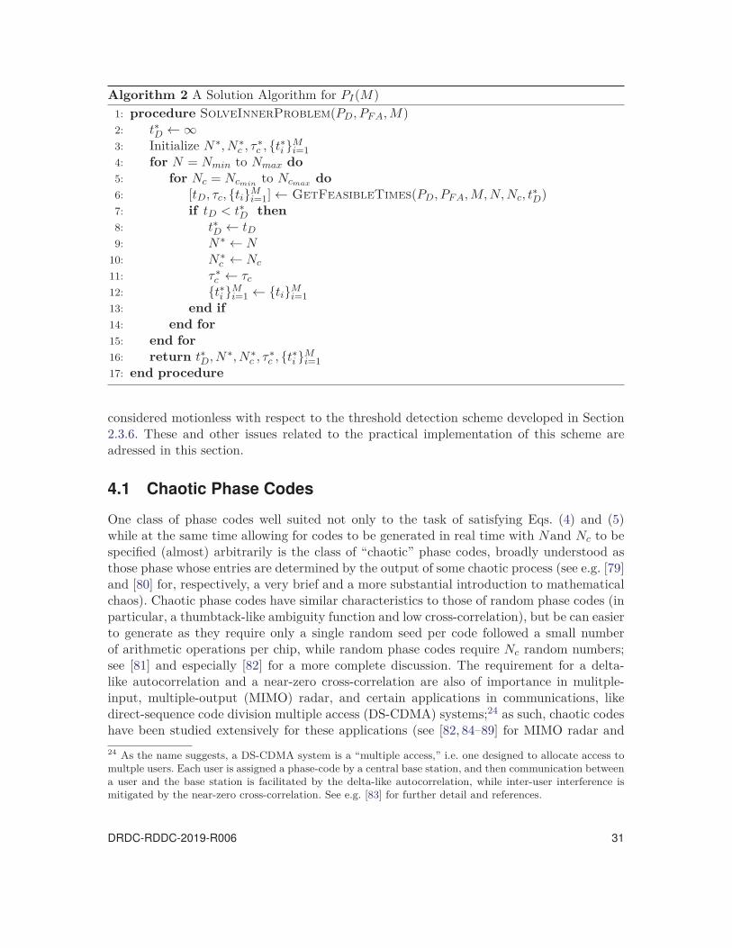
Algorithm 2 A Solution Algorithm for PI(M)1: procedure SolveInnerProblem(PD, PF A, M)2: t∗
D ← ∞3: Initialize N∗, N∗
c , τ∗c , {t∗
i }Mi=1
4: for N = Nmin to Nmax do5: for Nc = Ncmin to Ncmax do6: [tD, τc, {ti}M
i=1] ← GetFeasibleTimes(PD, PF A, M, N, Nc, t∗D)
7: if tD < t∗D then
8: t∗D ← tD
9: N∗ ← N10: N∗
c ← Nc
11: τ∗c ← τc
12: {t∗i }M
i=1 ← {ti}Mi=1
13: end if14: end for15: end for16: return t∗
D, N∗, N∗c , τ∗
c , {t∗i }M
i=117: end procedure
considered motionless with respect to the threshold detection scheme developed in Section2.3.6. These and other issues related to the practical implementation of this scheme areadressed in this section.
4.1 Chaotic Phase Codes
One class of phase codes well suited not only to the task of satisfying Eqs. (4) and (5)while at the same time allowing for codes to be generated in real time with Nand Nc to bespecified (almost) arbitrarily is the class of “chaotic” phase codes, broadly understood asthose phase whose entries are determined by the output of some chaotic process (see e.g. [79]and [80] for, respectively, a very brief and a more substantial introduction to mathematicalchaos). Chaotic phase codes have similar characteristics to those of random phase codes (inparticular, a thumbtack-like ambiguity function and low cross-correlation), but be can easierto generate as they require only a single random seed per code followed a small numberof arithmetic operations per chip, while random phase codes require Nc random numbers;see [81] and especially [82] for a more complete discussion. The requirement for a delta-like autocorrelation and a near-zero cross-correlation are also of importance in mulitple-input, multiple-output (MIMO) radar, and certain applications in communications, likedirect-sequence code division multiple access (DS-CDMA) systems;24 as such, chaotic codeshave been studied extensively for these applications (see [82, 84–89] for MIMO radar and24 As the name suggests, a DS-CDMA system is a “multiple access,” i.e. one designed to allocate access tomultple users. Each user is assigned a phase-code by a central base station, and then communication betweena user and the base station is facilitated by the delta-like autocorrelation, while inter-user interference ismitigated by the near-zero cross-correlation. See e.g. [83] for further detail and references.
DRDC-RDDC-2019-R006 31
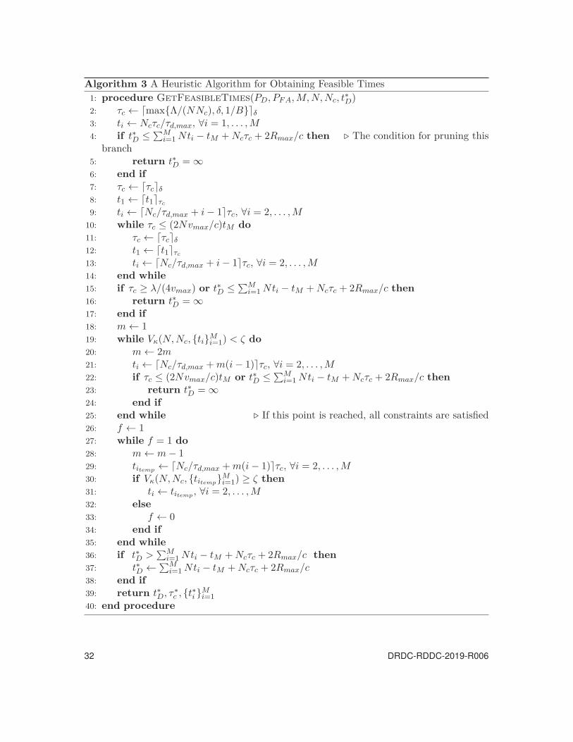
Algorithm 3 A Heuristic Algorithm for Obtaining Feasible Times1: procedure GetFeasibleTimes(PD, PF A, M, N, Nc, t∗
D)2: τc ← �max{Λ/(NNc), δ, 1/B}�δ
3: ti ← Ncτc/τd,max, ∀i = 1, . . . , M4: if t∗
D ≤ ∑Mi=1 Nti − tM + Ncτc + 2Rmax/c then � The condition for pruning this
branch5: return t∗
D = ∞6: end if7: τc ← �τc�δ
8: t1 ← �t1�τc
9: ti ← �Nc/τd,max + i − 1�τc, ∀i = 2, . . . , M10: while τc ≤ (2Nvmax/c)tM do11: τc ← �τc�δ
12: t1 ← �t1�τc
13: ti ← �Nc/τd,max + i − 1�τc, ∀i = 2, . . . , M14: end while15: if τc ≥ λ/(4vmax) or t∗
D ≤ ∑Mi=1 Nti − tM + Ncτc + 2Rmax/c then
16: return t∗D = ∞
17: end if18: m ← 119: while Vκ(N, Nc, {ti}M
i=1) < ζ do20: m ← 2m21: ti ← �Nc/τd,max + m(i − 1)�τc, ∀i = 2, . . . , M22: if τc ≤ (2Nvmax/c)tM or t∗
D ≤ ∑Mi=1 Nti − tM + Ncτc + 2Rmax/c then
23: return t∗D = ∞
24: end if25: end while � If this point is reached, all constraints are satisfied26: f ← 127: while f = 1 do28: m ← m − 129: titemp ← �Nc/τd,max + m(i − 1)�τc, ∀i = 2, . . . , M30: if Vκ(N, Nc, {titemp}M
i=1) ≥ ζ then31: ti ← titemp , ∀i = 2, . . . , M32: else33: f ← 034: end if35: end while36: if t∗
D >∑M
i=1 Nti − tM + Ncτc + 2Rmax/c then37: t∗
D ← ∑Mi=1 Nti − tM + Ncτc + 2Rmax/c
38: end if39: return t∗
D, τ∗c , {t∗
i }Mi=1
40: end procedure
32 DRDC-RDDC-2019-R006

[83,90–93] for DS-CDMA)
Of the above, [84, 85, 94] are particularly good candidates for use here, both in terms ofhaving good auto- and cross-correlation properties, but also in terms of being amenable toreal-time generation.25 However, for simplicity of implementation here, we follow [81] anduse a simple code generated by quantizing the so-called “logistic” map:
xn+1 = rxn(1 − xn) (54)
When the parameter r is set in the appropriate range (3.569945 · · · < r ≤ 4 [84]), theresulting sequence of xn values is chaotic; a value of r = 4 is used in this paper. A chaotic(biphase) code s = [s0, s1, . . . , sNc−1] is then generated by setting x0 to some random valuein (0, 1), computing x1, x2, . . . , xNc−1, and then setting si = 1 if xi ≤ 0.5 and xi = −1otherwise, for all indices i. While the size of the sidelobes obtained from such codes ingeneral decreases with the length of the code, in the numerical investigations conducted insupport of this paper (many of which are described below), typical peak sidelobe26 levelswere in the -26 dB to -32 dB neighbourhood for the parameters obtained from PO. Thismay be too large for practical instantiation, but it nevertheless suffices to establish a proof-of-concept for the scheme developed in this paper for the single target case; discussion onthis is otherwise deferred to Section 6.3.
4.2 A Hybrid Detector
Since the auto- and cross-correlation of the waves used in this scheme do not perfectly in-stantiate the properties in Eqs. (4) and (5), the threshold detector describe in Section 2.3.6is vulnerable to false alarms from the sidelobes of large target returns. In this section, ahybrid threshold/pseudo-CFAR27 detector is proposed that preserves the desired propertiesof the detector described in Section 2.3.6 (namely, the false alarm rate, the minimum guar-anteed probability of detection for maximally distant and small targets, and the strictlyimproved probability of detection for closer and smaller targets), while still preventing thisnew type of spurious detection.
Roughly, the hybrid detector uses the NP threshold of Section 2.3.6 in “noise-only” situa-tions, and a “pseudo-CFAR” detector if a pattern is detected that suggests large sidelobesmay trigger a false alarm. The term “pseudo-CFAR” is used because the detector has the25 Recall that this latter condition is important because the number of waveforms needed is not known inadvance, and optimizing a set waveforms once N is known is prohibitively complex for real-time operation;see [82] for further discussion. The alternative to the real-time condition is to have a large library of goodcodes of (nearly) every length computed in advance; although this can be difficult if N and Nc may be large,Section 6.3 discusses how this may be possible in practice.26 The word “sidelobe” will be used to refer any undesirable signal processing artefact that isn’t the mainspike of an autocorrelation, Rzz(0). This will include both range and frequency sidelobes of the returns ofa legitimate target and sidelobes due to cross-correlation of target returns due to two different pulses, theuse occurring in the latter case despite the fact that there is no feature of interest for the sidelobes to bebeside, except other sidelobes.27 Where “CFAR” denotes “constant false-alarm rate.”
DRDC-RDDC-2019-R006 33

same structure as that of an order-statistic CFAR detector, but does not contain the actualstatistical guarantee of a constant false-alarm rate. In principle, an actual (non-hybrid)CFAR detector could be used instead of this hybrid scheme, and indeed likely should in or-der to accommodate clutter in a practical scenario, but the hybrid scheme is valuable here tohighlight certain conceptual features of the problem that the use of a CFAR detector alonewould otherwise obscure. Note that there are two somewhat separate goals to consider here:the first is to understand the problem of minimizing dwell time while achieving specifiedunambiguous ranges and velocity measurements, while the second is to take steps towardsdeveloping a practically realizable scheme that can acomplish this. The threshold detectionapproach is useful for the former goal, as it allows for a more transparent understanding ofthe tensions between various parameters and variables in determining the dwell time, and,in allowing the problem to be studied under more “sterile” conditions, provides a standardby which future, more practical implementations can be measured against. Moreover, thesuccessful implementation of the pseudo-CFAR is contingent on an understanding of therole that realistic phase codes (i.e. ones that doesn’t satisfy Eqs. (4) and (5) exactly) playin the scheme. With a greater understanding of the problem abstractly, future work canfocus on practical implementation in a more intelligent and productive manner than wouldhave otherwise been possible.
The hybrid scheme functions specifically as follows. Suppose range cell i is the cell-under-test (CUT) for the presence of a target. Since the code of length Nc has an autocorrelation oflength 2Nc−1, an initial window consisting of the 2Nc−1 nearest28 lagging cells and 2Nc−1nearest leading cells is used in order to guarantee that, if the CUT contains target returns,then the rest of the associated returns will be in the window. Since the noise is assumed tobe Gaussian with a known variance, the sample variance s2 can be used to determine if thecontents of the window are likely to have been generated by noise alone. If they are unlikelyto have been noise-generated, then the pseudo-CFAR threshold is used instead of the NPthreshold. Details of the formal hypothesis test used in such a scenario (often referred to a“chi-squared” test of the (sample) variance) are readily found in textbooks of probabilityand statistics, see e.g. [95] (pp. 454–455). Letting yj denote the value of the j-th range cell,the corresponding test statistic
T =2(2Nc − 1)
NNcσ22
s2 =2
NNcσ
∑j
(yj − 1
4Nc − 2∑
k
yk
)2
(55)
has a χ2 (chi-squared) distribution with 4Nc − 3 degrees of freedom. The probability thatnoise alone would generate a value of T or less is given by the integral of the correspondingχ2 probability density function from 0 to T . In the traditional formal hypothesis test, ifthis integrated value is sufficiently large (i.e. greater than 1-α for the test significance levelα, usually 0.01, 0.05, or 0.10), then the “null” hypothesis that the sample data is generatedfrom a process with variance NNcσ/2 is rejected.28 Note that since only point targets are considered here, and since the phase codes used here have narrowmainlobes, no guard cells are used; nevertheless the use of guard cells in practical scenarios is a topic worthyof further study.
34 DRDC-RDDC-2019-R006

A slightly modified approach is used here which was found to be slightly more useful aftersome initial testing. Note that the window above does not include the CUT itself in per-forming the variance test. When the CUT is included in the test window, and either targetreturns or large sidleobes are in the CUT, the null hypothesis is almost always rejected,which would trigger the pseudo-CFAR threshold. While this is good for avoiding detectionof spurious sidelobes for closer targets and sufficient for detecting legitimate returns of closetargets, it is bad for detecting legitimate returns from distant targets which, despite beingabove the NP threshold, are only slightly above the noise level and are inevitably obscuredby the pseudo-CFAR threshold. Fortunately, cases where this happens are easy to identify,as their test statistic are comparatively small: the autocorrelation sidelobes surrounding thelegitimate spike are small relative to noise for distant targets, and so the sidelobes plus thenoise are essentially indistinguishable from noise. After some initial experiments, it was de-termined that a value of 0.02 worked well: if the test statistic yielded an integral below thisvalue, the CUT should not be included in the test window, but otherwise it should. Withthe test window determined, the formal hypothesis test above is conducted with significancelevel α = 0.95. The full procedure is summarized in Algorithm 4.
Algorithm 4 The Hybrid NP/Pseudo-CFAR Detector Threshold Selection Scheme1: procedure HybridDetectorThreshold(y, i)2: � Let y denote the frequency-compensated and match-filtered
data and i denote the index of the CUT. The NP threshold, TNP , CFAR multiple forthe CPI, αCF AR, and other system parameters are assumed to be already known.
3: WT est ← [yi−2Nc+1, . . . , yi−1, yi+1, . . . , yi+2Nc−1]4: l ← 4Nc − 25: s2 ← 1
l−1∑
j∈WT est
(yj − 1
l
∑k∈WT est
yk
)2
6: T ← lNNcσ2
2s2
7: ω ← ∫ T0
x(l−1)/2−1e−x/2
2(l−1)/2Γ((l−1)/2)dx � Γ(x) is the standard gamma function (see [95], pp 170)8: if ω > 0.02 then � The mainlobe is included in the test window9: WT est ← [yi−2Nc+1, . . . , yi−1, yi, yi+1, . . . , yi+2Nc−1]
10: l ← 4Nc − 211: s2 ← 1
l−1∑
j∈WT est
(yj − 1
l
∑k∈WT est
yk
)2
12: T ← lNNcσ2
2s2
13: ω ← ∫ T0
x(l−1)/2−1e−x/2
2(l−1)/2Γ((l−1)/2)dx
14: end if15: if ω > 0.95 then16: WCF AR ← [yi−Nc+1, . . . , yi−1, yi+1, . . . , yi+Nc−1]17: T0 ← max{αCF AR max{WCF AR}, TNP }18: else19: T0 ← TNP
20: end if21: end procedure
DRDC-RDDC-2019-R006 35

Algorithm 4 also shows explicitly how the pseudo-CFAR threshold value is determined. Aspreviously mentioned, it mimics an order-statistic CFAR detector, insofar as the thresholdis set as some multiple of the k-th largest value in the CFAR test window. Since only singlepoint targets are considered in this paper, k = 1 suffices, but for practical multiple-targetscenarios, a larger k, e.g. k = �Nc/4� [2], in order to minimize the likelihood of maskingother targets. In a true order-statistic CFAR detector, the multiple is chosen to maintainthe desired false-alarm rate, whereas here, a more heuristic calculation is used. Prior totransmission of the first phase code of a CPI, all N phase codes for a CPI are generated;their respective autocorrelations are then calculated, and the autocorrelations are addedup, as if integrating the returns of a target. The ratio of the mainlobe to the peak sidelobeof the resulting form can then be calculated, and then a fraction of this value (60% is usedbelow) is used as the CFAR multiple for that CPI. This method guarantees detection oflegitimate returns if the sidelobes of the wave are larger than the noise and if the pseudo-CFAR threshold is activated as per Algorithm 4 because the sidelobes are fixed and knowna priori, whereas typical clutter is only characterized statistically. This property of thepseudo-CFAR is crucial to allow the hybrid detection scheme to maintain the desirableproperty of the NP-detection (only) scheme. But before this is discussed, we note that the60% is somewhat arbitrary and discuss the factors determining its choice. Anything below100% will suffice for the detection of legitimate targets for the situation discussed above, butlarger values hedge against the spurious detection of sidelobes, while lower values decreasethe severity of masking of multiple targets. The value 60% was sufficient for the experimentsconducted here, but for a practical scheme, more robust simulation and validation beyondthe scope of this paper would have to be performed. Note also that the CFAR windowincludes only the Nc − 1 leading and Nc − 1 lagging cells, compared to the 2Nc − 1 usedfor both in the hypothesis testing. The latter size is used to ensure that if the CUT isany sidelobe in some auto- or cross- correlation returns, then all other sidelobes (and themainlobe if applicable) are included in the test, but a window of this size is not neededwhen actually computing the CFAR threshold.
In Section 2.3.6, the NP threshold detection scheme was presented as having three desirablefeatures: a constant false alarm probability PF A, a minimum probability of detection PD
for maximally distant and small targets (provided no eclipsing and range migration occurs),and a strictly better probability of detection for closer and/or larger targets (again, providedno eclipsing or migration). It is desirable to maintain these properties despite the use ofnon-ideal phase codes and a hybrid detection scheme. This can be done if the following istrue of the (or any other) hybrid detector:
1. When a sidelobe in the CUT passes the NP threshold, the detector always uses thepseudo-CFAR threshold.
2. The pseudo-CFAR multiple is large enough so that a sidelobe in the CUT is alwaysless than the pseudo-CFAR threshold when a sidelobe is used as the CFAR test value(i.e. the largest value in the test window in this case, or the k-th largest value in thetest window for a k-th order order-statistic CFAR is used).
36 DRDC-RDDC-2019-R006

3. The pseudo-CFAR multiple is small enough to guarantee that a legitimate autocor-relation mainlobe is always greater than the pseudo-CFAR threshold when a sidelobeis used as the CFAR test value.
4. When (and only when) a legitimate target is very small or far away such that its auto-correlation sidelobes are much smaller than (i.e. “below”) the noise, the NP thresholdis always used.
It is straightforward to see how these four characteristics maintain the desired properties.First, the initial two items ensure that pseudo-CFAR portion of the hybrid detector isguaranteed to prevent the detection of sidelobes, so the false alarm rate does not increase.Next, the probability of detection for maximally distant and small targets does not decreasefrom PD as the fourth item guarantees that the hybrid scheme uses the NP threshold inthat circumstance. Finally, the probability of detection for closer/larger targets is better:when the sidelobes are much smaller than the noise, the fourth item dictates that the NPthreshold is used, so detection occurs in the ordinary way, while in the case where the targetsidelobes are sufficiently large, the pseudo-CFAR threshold is guaranteed to be able to detectthe target above its sidelobes by the third item. While the hybrid detector proposed here isthe right kind of detector to satisfy these four criteria, the problem remains to determinethe degree to which it actually does. Sections 6.3 and 6.4 contain further discussion onwaveforms and detectors in practical contexts.
4.3 Frequency Compensation
It was assumed in Section 2.3.6 that some form of frequency (i.e. velocity) compensationwould be performed at the receiver such that detection could safely be assumed to beperformed on motionless targets. This section details the method for performing frequencycompensation at a single given frequency. Target detection for targets at all velocities canthen be done as detection of targets at a single velocity, for all velocities of interest. Anadvantage of this approach is that, assuming sufficient computational resources, these single-velocity computations can be performed in parallel. The velocities of interest are determinedby the Doppler-tolerance ( [2] pp. 816–817) of the chaotic phase codes, a characteristic whosedetailed study is beyond the scope of this paper but should be addressed in future work tofacilitate practical implementation.
Recall Eq. (6), reprinted below, which describes the form a sample containing returns of atarget located at R0 at t = 0 and travelling at a speed v towards the radar:
y = Asie−j 2π
λ (2(R0−vt)) + z = Asie−j 4π
λR0ej2π 2v
λt + z
Consider the second exponential term on the right hand side of the second equality sign.The time t at which the sample is taken is necessarily an integer multiple of the sample timeτc, and so it is clear that with each successive sample, the phase of the returns increases by4πvτc/λ. This constant change of phase is the Doppler shift. A simple method of Dopplercompensation is thus to “undo” the multiplication of these phase shifting exponentials by
DRDC-RDDC-2019-R006 37

multiplying each successive sample by their complex conjugates. Specifically, to compensatefor a velocity v, the vector of baseband samples y should be multiplied elementwise as
[y0, y1, y2, . . . , y�2Rmax/(cτc)�] ⊗ [1, e−j2π 2vλ
τc , e−j2π 2vλ
2τc , . . . , e−j2π 2vλ
� 2Rmaxcτc
�τc ], (56)
where ⊗ denotes elementwise multiplication. The resulting form of the hypothetical samplein Eq. (6) is then
y = Asie−j 4π
λR0 + ze−j2π 2v
λt,
where there is no longer a Doppler shift in the signal. Note that, while the noise samplez has been multiplied by a complex exponential, this does not change the statistics of thenoise, as this operation corresponds to the rotation of a circularly-symmetric probabilitydensity function in the complex plane.
This approach is desirable for its computational simplicity, but has a drawback. Once fre-quency compensation has occurred, pulses are integrated within a CPI via matched filteringof individual pulses, followed by the addition of the matched filtered pulses and the takingof the real part of the resulting sum. Although this is done digitally, the mathematics ofanalog signals is more straightforward and equally illuminating; this integration can thusbe represented as
Re{∫ ∞
−∞|y(t)|2dt
}, (57)
i.e. the real part of the zero-delay, zero-frequency value of the ambiguity function χ(τ, ν)(see [96] Ch. 3) of the (baseband) of the transmitted waveform y(t). Now since y(t) iscomposed of a train of phase-coded pulses, |y(t)|2 is a simple train of square pulses and thecomputation in Eq. (57) is straightforwardly found to be sinc pulse with periodic repetition.When the frequency compensation method described above is used, however, each CPI canno longer be considered as starting at its own relative t = 0. Instead, time information isencoded in the multiple of τc used in the complex exponent, which indentifies how muchtime-shifting each CPI undergoes relative to the beginning of the first CPI. That a timeshifting of tshift introduces frequency artefacts is evident from the zero-delay cut of theambiguity function:
χtshift(0, ν) =
∫ ∞
−∞|y(t − tshift)|2ej2πνtdt
=∫ ∞
−∞|y(t′)|2ej2πν(t′+tshift)dt′, letting t′ = t − tshift,
= ej2πνtshift
∫ ∞
−∞|y(t′)|2ej2πνt′
dt, (58)
= ej2πνtshiftχ0(0, ν) (59)
Explicitly, Eq. (59) shows that the time-shifted version of the zero-delay ambiguity functionis equal to the ordinary (non-shifted) zero-delay ambiguity function multiplied by a complexexponential. When the real part of the signal is taken, that complex exponential becomescos(2πνtshift), and so it is clear that the sinc-shaped ambiguity function of the ordinary
38 DRDC-RDDC-2019-R006
signal will be modulated in frequency by this cosine. At the correct frequency (ν = 0, sincefrequency compensation has already occurred), the mainlobe of the sinc does not have it’sheight reduced since cos(0) = 1, so this won’t affect detection of legitimate targets. It does,however, cause the presence of large sidelobes in other frequency bins, and this modulationbecomes more severe for later CPI as tshift is larger for each successive CPI. It is thuspossible that these sidelobes generate spurious detections at the same range but differentfrequencies as a legitimate target if the receiver does not account for these artefacts. In thissimulations performed for this work, since only single targets are considered, these sidelobes(whose specific location relative to a target’s velocity can be known thanks to calculationslike Eq. (59)) - see Annex A for an example) are zeroed-out. In practice, this would run therisk of masking other legitimate targets at different speeds but the same range, so a moresophisticated approach would subtract out the effect of sidelobes, but the development ofsuch an algorithm is beyond the scope of this paper.
4.4 Clustering Algorithm
The use of a clustering algorithm has been discussed several times previously. It has beennoted that the benefits of a clustering algorithm include improved robustness to measure-ment error and ghosting (Section 1.2.1) and the tolerance of range migration between CPI(Section 2.3.8), while a drawback is the possibility of slightly increased vulnerability to falsealarms (Section 2.3.6). The simple clustering algorithm used here, following [9], uses a fixed-window approach. Specifically, if within a fixed window of range/velocity cells centered at adetection (i.e. a range/velocity cell with a value exceeding the threshold for that cell), thereare other detections from at least one other CPI,29 then that window contains a legitimatecluster corresponding to a possible target. By iterating over all detections to determine therespective clusters for each, a list of potential targets is formed, from which the presence ofreal targets must be determined.
Two principles guide this latter process: first, that the detection with the largest magnitudeis more likely to be due to a legitimate target than to a spurious noise or sidelobe detection,and second, that legitimate targets tend to have more detections in a cluster (see Section1.2.1). The cluster selection scheme then proceeds as follows. The detection with the largestmagnitude is determined, and any other detections with heights within, say, 5% are iden-tified as well. Among these detections, the detection having the greatest total number ofdetections in its cluster is declared to be a legitimate target.30 The range and velocity ofthe target is then taken as the arithmetic average of the ranges and velocities of the respec-tive values in the cluster. The detections in the cluster, along with detections potentiallycorresponding to frequency artefacts of the detection (see Section 4.3), are removed from29 Although this is true only for M ≥ 3. For M < 3, only one CPI is needed; see Section 2.3.6.30 This implicitly makes the judgement that, say, a detection with nominal magnitude 1 and two otherdetections in its cluster is less likely to be the location of a legitimate target than a detection with nominalheight 0.98 and three other detections in its cluster. In the experiments conducted below for the singletarget case, it was found that there is almost never a second detection with a height within 5% of the largestdetection, so in that context the point is largely moot.
DRDC-RDDC-2019-R006 39
the global list of detections, and the above process is repeated until there are no legitimateclusters left.
The window used in the simulation below had a size of ±3 range cells and ±�1/(Nt1fsep)�velocity cells, where fsep is the maximum frequency resolution allowed in the receiver. Theformer value is used because a target can migrate at most 3 range cells in 3 CPI, andnearly all the simulations below all had M ≤ 3; a more sophisticated choice is to usethe optimal value of M obtained from the optimization problem. The latter value is thenumber of cells in the widest frequency-domain mainlobe of all CPI (see Section 4.3). Thesechoices are heuristic, but the development of more sophisticated approaches (e.g. based offof techniques discussed in Section 1.2.1) are beyond the scope of this paper.
5 Numerical Evaluation and Simulation5.1 Optimization Problem Solution
In this section, the solution algorithm developed in Section 3 is implemented and used toexplore the optimization problem in Eqs.(7a)–(7d) numerically. The baseline parametersused are listed in Table 1, i.e. unless otherwise stated, the parameter listed in the tableis the one used for the problem. Note the inclusion of a term, “radar quality,” which is acertain ratio of the previous six parameters. This value is of greater significance than the sixparameters in isolation, as, mathematically, it will not matter if an increase in “quality” isdue to an increase in antenna gains, a decrease in system losses, or whatever else, in termsof how the dwell time is affected.
First, Figure 5 shows how variation in the nominal visibility ζ affects total dwell time. Notethat data points are not evenly spaced, as areas of greater interest warrant more data points,and each point is annotated with the optimal M value for that solution. For ζ = 0.85, itis easy for the solution algorithm to satisfy the visibility constraint with M = 1 since themaximum duty cycle is td,max = 0.1. As the value of ζ increases, however, the duty cycle ofthe wave used in the M = 1 case becomes increasingly small. The value of td,max and theconstraint Eq. (35c) require that the smallest possible value for a1 in t1 = a1τc is 10Nc. Forζ = 0.90, it turns out that a1 = 10. ¯1188Nc, and for ζ = 0.925, a1 = 13.36Nc. With Ncτc
essentially fixed by the required energy-on-target (NNcτc = 3.6865·10−4 for the former caseand NNcτc = 3.696 · 10−4 for the latter), this means that the PRIs simply become longer inorder to accommodate the visibilty constraint, lengthening the dwell time. By ζ = 0.9375,it simply becomes more efficient to use 3 CPI. Even though there are more CPI, each oneis more time-efficient (a1 = 10Nc, a2 = 10.125Nc, a3 = 10.25Nc) and has a less stringentenergy-on-target requirement (NNcτc = 1.74 · 10−4) than the only CPI for the M = 1 case(a1 ≈ 16.2Nc and NNcτc = 3.6894 ·10−4 respectively), and so on balance, the multiple-PRFapproach yields a smaller dwell time in this case. As the visibility condition becomes morestrict (ζ ≥ 0.9375), the three CPI solution accommodates the change with only a minorincrease in dwell time: the dwell time increase from ζ = 0.9375 to ζ = 0.975 is only 0.8% .Only a small change in the relative sizes of the ai values is needed to get a few extra percent
40 DRDC-RDDC-2019-R006
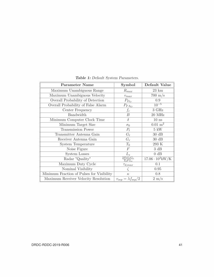
Table 1: Default System Parameters.
Parameter Name Symbol Default ValueMaximum Unambiguous Range Rmax 23 km
Maximum Unambiguous Velocity vmax 700 m/sOverall Probability of Detection PDO
0.9Overall Probability of False Alarm PF AO
10−5
Center Frequency fc 3 GHzBandwidth B 20 MHz
Minimum Computer Clock Time δ 10 nsMinimum Target Size σ0 0.01 m2
Transmission Power Pt 5 kWTransmitter Antenna Gain Gt 30 dB
Receiver Antenna Gain Gr 30 dBSystem Temperature T0 293 K
Noise Figure F 3 dBSystem Losses Ls 0 dB
Radar "Quality" 2PtGtGrT0F Ls
17.06 · 103kW/KMaximum Duty Cycle τd,max 0.1
Nominal Visibility ζ 0.95Minimum Fraction of Pulses for Visibility κ 0.8Maximum Receiver Velocity Resolution vsep = λfsep/2 2 m/s
DRDC-RDDC-2019-R006 41
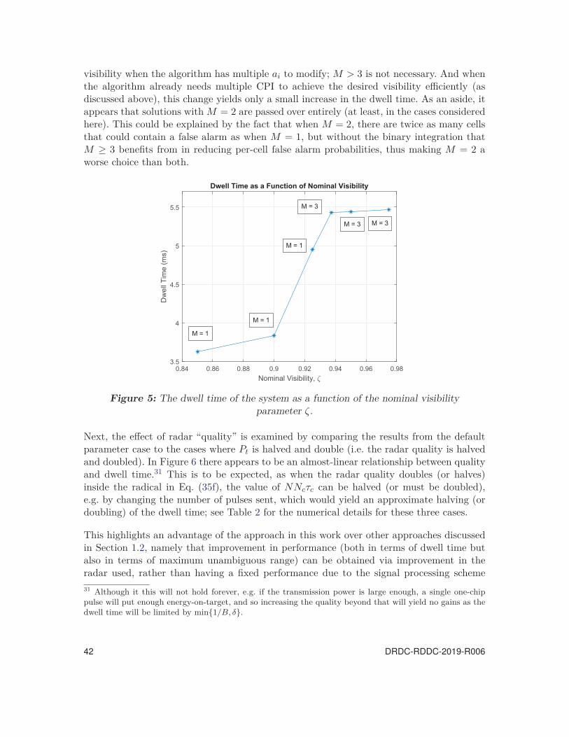
visibility when the algorithm has multiple ai to modify; M > 3 is not necessary. And whenthe algorithm already needs multiple CPI to achieve the desired visibility efficiently (asdiscussed above), this change yields only a small increase in the dwell time. As an aside, itappears that solutions with M = 2 are passed over entirely (at least, in the cases consideredhere). This could be explained by the fact that when M = 2, there are twice as many cellsthat could contain a false alarm as when M = 1, but without the binary integration thatM ≥ 3 benefits from in reducing per-cell false alarm probabilities, thus making M = 2 aworse choice than both.
0.84 0.86 0.88 0.9 0.92 0.94 0.96 0.98Nominal Visibility,
3.5
4
4.5
5
5.5
Dw
ell T
ime
(ms)
Dwell Time as a Function of Nominal Visibility
M = 1
M = 1
M = 3
M = 3 M = 3
M = 1
Figure 5: The dwell time of the system as a function of the nominal visibilityparameter ζ.
Next, the effect of radar “quality” is examined by comparing the results from the defaultparameter case to the cases where Pt is halved and double (i.e. the radar quality is halvedand doubled). In Figure 6 there appears to be an almost-linear relationship between qualityand dwell time.31 This is to be expected, as when the radar quality doubles (or halves)inside the radical in Eq. (35f), the value of NNcτc can be halved (or must be doubled),e.g. by changing the number of pulses sent, which would yield an approximate halving (ordoubling) of the dwell time; see Table 2 for the numerical details for these three cases.
This highlights an advantage of the approach in this work over other approaches discussedin Section 1.2, namely that improvement in performance (both in terms of dwell time butalso in terms of maximum unambiguous range) can be obtained via improvement in theradar used, rather than having a fixed performance due to the signal processing scheme31 Although it this will not hold forever, e.g. if the transmission power is large enough, a single one-chippulse will put enough energy-on-target, and so increasing the quality beyond that will yield no gains as thedwell time will be limited by min{1/B, δ}.
42 DRDC-RDDC-2019-R006

2 3 4 5 6 7 8 9 10 11 12Transmission Power, Pt (kW)
2
3
4
5
6
7
8
9
10
11
12
Dw
ell T
ime
(ms)
Dwell Time as a Function of Radar "Quality"
Figure 6: The dwell time of the system as a function of the radar quality, which here isvaried by varying the transmission power Pt.
Table 2: The Almost-Linear Relationship Between Radar Quality and Dwell Time.
Pt (kW) tD (ms) N Nc τc (ns) NNcτc · 104
2.5 10.732533 303 23 50 3.48455 5.4404733 145 20 60 1.740010 2.792833 58 30 50 0.8700
DRDC-RDDC-2019-R006 43

Table 3: Energy-on-Target Variation with Bandwidth.
B (Hz) tD (ms) N Nc τc (ns) NNcτc · 104
2 5.28433 32 10 500 1.6005 5.24733 69 10 240 1.65610 5.321733 106 16 100 1.69620 5.4404733 145 20 60 1.740
used. Figure 6 shows the improvement of dwell time, but the improvement in unambiguousrange (for a fixed dwell time) can be seen using the same reasoning. By increasing Rmax
by some factor, if radar quality is improved by that factor raised to the fourth power, thenthe dwell time will stay approximately constant;32 see Section 6.5 for further detail.
The next parameter variable of interest is bandwidth. A priori, one could imagine that forlarge bandwidths, variation in bandwidth will not result in a significant change in dwelltime, since a change in τc can be accomodated by a changes in N and Nc such that NNcτc
is relatively constant. Indeed, Figure 7 shows that there is not much significant change overlarge ranges of bandwidth, although this statement has important qualifications.
106 107
Bandwidth, Hz
3
3.5
4
4.5
5
5.5
6
6.5
Dw
ell T
ime
(ms)
Dwell Time as a Function of Bandwidth
Figure 7: The dwell time of the system as a function of the available bandwidth.
First, note that when bandwidth is increased indefinitely, no effect is had on dwell timebecause the limiting factor on a small τc becomes δ. More importantly, however, we notethat reducing the bandwidth from 20 MHz to 2 MHz actually (slightly) improved theperformance. This highlights a shortcoming of the particular solution algorithm used in32 The 2Rmax/c term will necessarily increase, but since that typically small relative to the total dwell time(e.g. 0.1533 ms at 23 km), this will not result in a significant increase in dwell time.
44 DRDC-RDDC-2019-R006
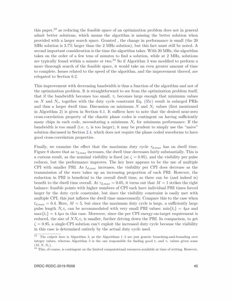
this paper,33 as reducing the feasible space of an optimization problem does not in generaladmit better solutions, which means the algorithm is missing the better solution whenprovided with a larger search space. Granted , the change in performance is small (the 20MHz solution is 3.7% larger than the 2 MHz solution), but this fact must still be noted. Asecond important consideration is the time the algorithm takes. With 20 MHz, the algorithmtakes on the order of a few tens of minutes to find a solution, while at 2 MHz, solutionsare typically found within a minute or two.34 So if Algorithm 3 was modified to perform amore thorough search of the feasible space, it would take an even greater amount of timeto complete. Issues related to the speed of the algorithm, and the improvement thereof, arerelegated to Section 6.2.
This improvement with decreasing bandwidth is thus a function of the algorithm and not ofthe optimization problem. It is straightforward to see from the optimization problem itself,that if the bandwidth becomes too small, τc becomes large enough that minimum valueson N and Nc, together with the duty cycle constraint Eq. (35c) result in enlarged PRIsand thus a larger dwell time. Discussion on minimum N and Nc values (first mentionedin Algorithm 2) is given in Section 6.1. It suffices here to note that the desired near-zerocross-correlation property of the chaotic phase codes is contingent on having sufficientlymany chips in each code, necessitating a minimum Nc for minimum performance. If thebandwidth is too small (i.e. τc is too larger), it may be prudent to simply use the “naive”solution discussed in Section 2.4, which does not require the phase coded waveforms to havegood cross-correlation properties.
Finally, we examine the effect that the maximum duty cycle τd,max has on dwell time.Figure 8 shows that as τd,max increases, the dwell time decreases fairly substantially. This isa curious result, as the nominal visibility is fixed (at ζ = 0.95), and the visibility per pulsereduces, but the performance improves. The key here appears to be the use of multipleCPI with smaller PRI. As td,max increases, the visibility per CPI does decrease as thetransmission of the wave takes up an increasing proportion of each PRI. However, thereduction in PRI is beneficial to the overall dwell time, so there can be (and indeed is)benefit to the dwell time overall. At τd,max = 0.05, it turns out that M = 1 strikes the rightbalance: feasible points with higher numbers of CPI each have individual PRI times forcedlarger by the duty cycle constraint, but since the visibility constraint is easily met withmultiple CPI, this just inflates the dwell time unnecessarily. Compare this to the case whentd,max = 0.4. Here, M = 5, but since the maximum duty cycle is large, a sufficiently largepulse length Ncτc can be accommodated with very small PRI values: min{ti} = 4μs andmax{ti} = 4.4μs in this case. Moreover, since the per CPI energy-on-target requirement isreduced, the size of NNcτc is smaller, further driving down the PRI. In comparison, to getζ = 0.95, a single-CPI solution can’t exploit the increased duty cycle because the visibilityin this case is determined entirely by the actual duty cycle used.33 The culprit here is Algorithm 3, as the Algorithms 1–2 are just generic branching-and-bounding overinteger values, whereas Algorithm 3 is the one responsible for finding good ti and τc values given some(M, N, Nc).34 This, of course, is contingent on the limited computational resources available at time of writing. However,
DRDC-RDDC-2019-R006 45
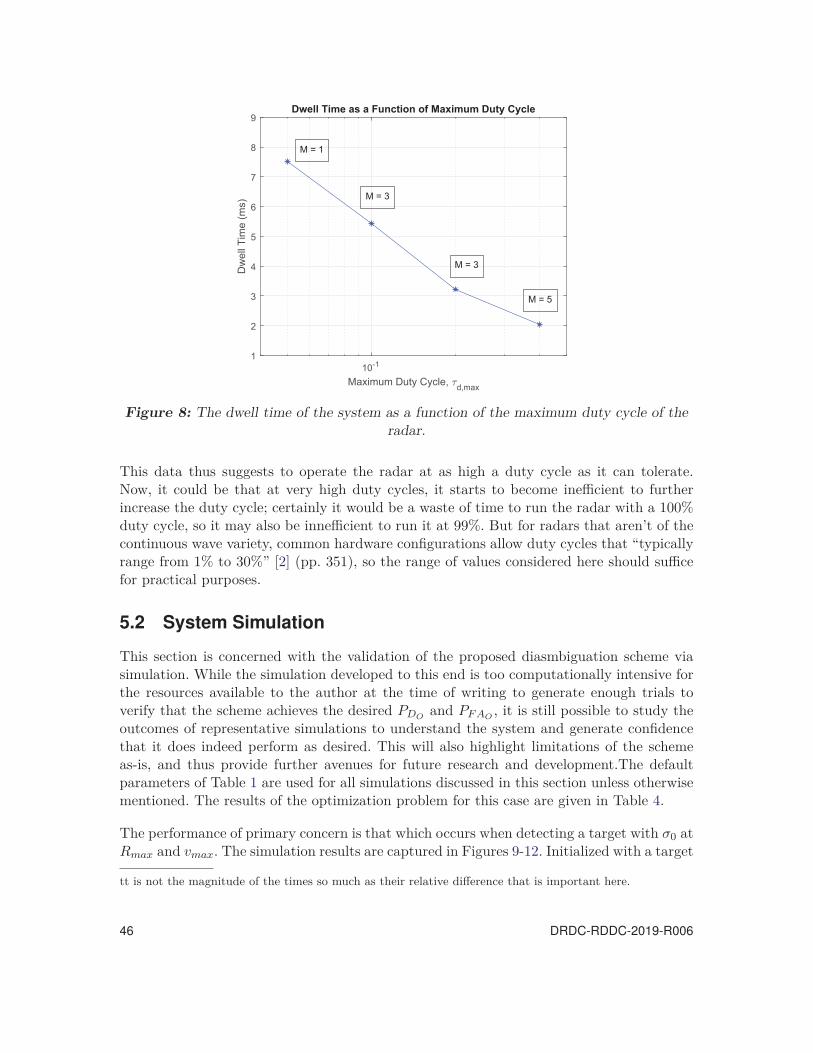
10-1
Maximum Duty Cycle, d,max
1
2
3
4
5
6
7
8
9
Dw
ell T
ime
(ms)
Dwell Time as a Function of Maximum Duty Cycle
M = 1
M = 3
M = 3
M = 5
Figure 8: The dwell time of the system as a function of the maximum duty cycle of theradar.
This data thus suggests to operate the radar at as high a duty cycle as it can tolerate.Now, it could be that at very high duty cycles, it starts to become inefficient to furtherincrease the duty cycle; certainly it would be a waste of time to run the radar with a 100%duty cycle, so it may also be innefficient to run it at 99%. But for radars that aren’t of thecontinuous wave variety, common hardware configurations allow duty cycles that “typicallyrange from 1% to 30%” [2] (pp. 351), so the range of values considered here should sufficefor practical purposes.
5.2 System Simulation
This section is concerned with the validation of the proposed diasmbiguation scheme viasimulation. While the simulation developed to this end is too computationally intensive forthe resources available to the author at the time of writing to generate enough trials toverify that the scheme achieves the desired PDO
and PF AO, it is still possible to study the
outcomes of representative simulations to understand the system and generate confidencethat it does indeed perform as desired. This will also highlight limitations of the schemeas-is, and thus provide further avenues for future research and development.The defaultparameters of Table 1 are used for all simulations discussed in this section unless otherwisementioned. The results of the optimization problem for this case are given in Table 4.
The performance of primary concern is that which occurs when detecting a target with σ0 atRmax and vmax. The simulation results are captured in Figures 9-12. Initialized with a target
tt is not the magnitude of the times so much as their relative difference that is important here.
46 DRDC-RDDC-2019-R006
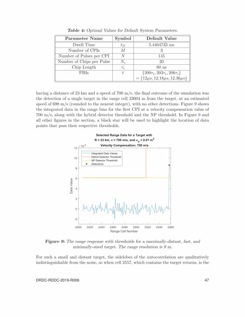
Table 4: Optimal Values for Default System Parameters.
Parameter Name Symbol Default ValueDwell Time tD 5.4404733 ms
Number of CPIs M 3Number of Pulses per CPI N 145Number of Chips per Pulse Nc 20
Chip Length τc 60 nsPRIs t {200τc, 203τc, 206τc}
= {12μs, 12.18μs, 12.36μs}
having a distance of 23 km and a speed of 700 m/s, the final outcome of the simulation wasthe detection of a single target in the range cell 23004 m from the target, at an estimatedspeed of 698 m/s (rounded to the nearest integer), with no other detections. Figure 9 showsthe integrated data in the range bins for the first CPI at a velocity compensation value of700 m/s, along with the hybrid detector threshold and the NP threshold. In Figure 9 andall other figures in the section, a black star will be used to highlight the location of datapoints that pass their respective thresholds.
2400 2420 2440 2460 2480 2500 2520 2540 2560Range Cell Number
-2
0
2
4
6
8
10
12
Dat
a V
alue
10-5
Selected Range Data for a Target with R = 23 km, v = 700 m/s, and 0 = 0.01 m2
Velocity Compensation: 700 m/s
Integrated Data ValuesHybrid Detector ThresholdNP Detector ThresholdDetections
Figure 9: The range response with thresholds for a maximally-distant, fast, andminimally-sized target. The range resolution is 9 m.
For such a small and distant target, the sidelobes of the autocorrelation are qualitativelyindistinguishable from the noise, so when cell 2557, which contains the target returns, is the
DRDC-RDDC-2019-R006 47

CUT, the hybrid detector uses the NP threshold, which the returns easily exceed. However,from cells 2556 to just below cell 2520, the target returns cause the hybrid detector todeclare that sidelobes are present, and so the pseudo-CFAR threshold detector is used. TheCFAR factor, much greater than unity, is multiplied by the target returns, thus causingthe pseudo-CFAR to be so large it is outside of the figure. Given that this masked distancecorresponds to about 40 ∗ 9 m = 360 m of real space (on both sides of the target if it isfurther in the interior of the unambiguous range) motivates the use of a more advancedCFAR structure like the k-th order order-statistic CFAR detector discussed in Section 4.2.While in the single-target case it is tolerable, in a practical scenario, multiple targets ofinterest may be close by and thus a more discriminating detector would be required.
Figures 10–12 show the frequency response at the 2557-th range cell for the three CPIsrespectively along with the threshold values in that range/velocity bin. In Figure 9, thewide mainlobe of the sinc-shaped response in the first CPI is shown to result in detectionsat four consecutive velocity values below the correct one. With the additional modulationin the second CPI, shown in Figure 11, the mainlobe is thinner and thus results only inone additional detection. However, the modulation in the third CPI (Figure 12) causes anadditional detection not immediately next to the correct one, but at a frequency sidelobe10 m/s down. As discussed in Sections 4.3 and 4.4 these sidelobes and additional detectionscan be accounted for without the reciever considering them false alarms and to any mitigatepotential masking. The clustering algorithm considers the detections of the mainlobe to bea part of the cluster of the legitimate target, while the sidelobe detection in the third CPIis suppressed once the real target is correctly located at the 700 m/s velocity bin. In thissimulation, of the nine total detections prior to clustering and supression, none remainedoutstanding after clustering and supression. This is the ideal outcome, as outstanding indi-vidual detections either are false alarms (if M < 3) or make the system more vulnerable tofalse alarms (if M ≥ 3). The arithmetic average of the detections in the cluster yields anestimate just under 698 m/s, which is lower than the true value of 700 m/s, but when tar-gets are further into the interior of the unambiguous velocity set, the additional detectionsare symmetric about the correct value and so the estimate and correct value end up nearlyidentical.
Now we consider the same exercise for a target at a distance of 3824 m from the radar35
and with a speed of 650 m/s. The closer distance will allow for a more careful examinationof the effects of sidelobes, both autocorrelation and cross-correlation, while the lower speedallows the symmetry of the frequency response to be more easily observed. Figure 13 showsthe range response centered at the range cell containing the target. Here, the sidelobes ofthe autocorrelation are qualitatively distinct from the noise, and trigger the pseudo-CFARthreshold of the hybrid detector. It is quite clear that the existing pseudo-CFAR approachwould be unnacceptable in the multiple-target case due to the degree to which a single targetwould mask other nearby targets; however, the variation in the hybrid detector thresholdheight suggests that a k-th order order-statistic CFAR structure with a k value of 3 or 435 This distance, and other considered below, are chosen in part because they will not result in any rangemigration of the target during the dwell.
48 DRDC-RDDC-2019-R006
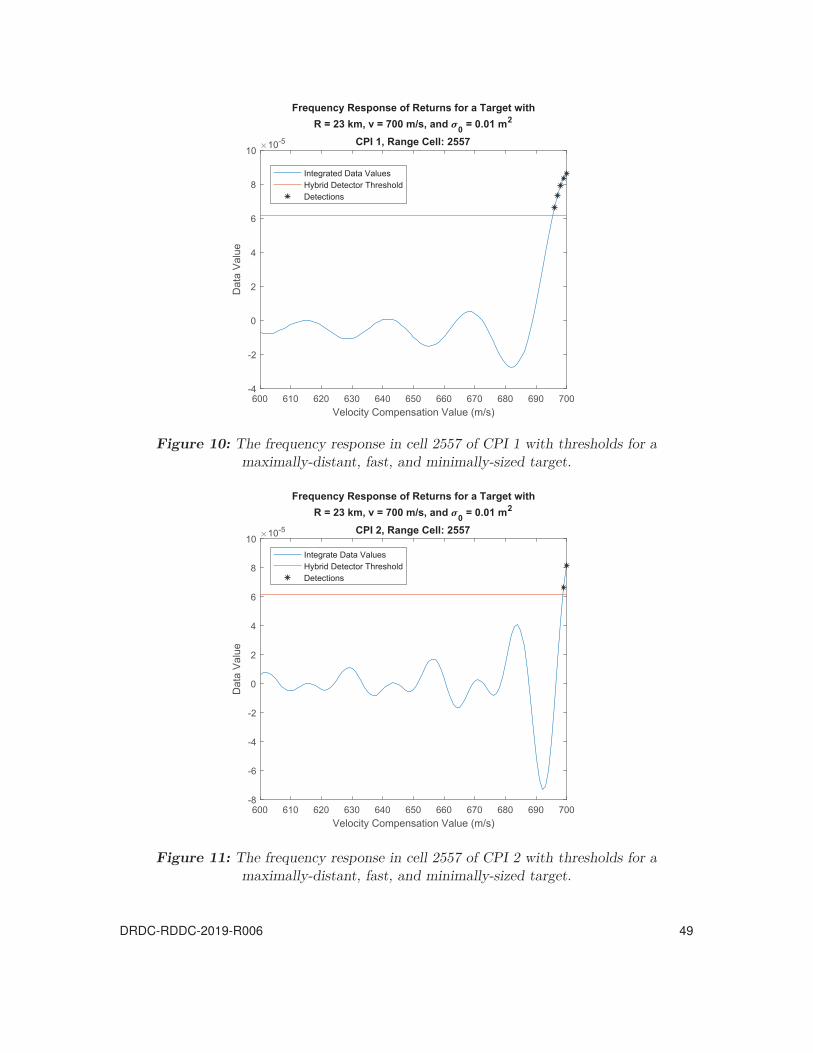
600 610 620 630 640 650 660 670 680 690 700Velocity Compensation Value (m/s)
-4
-2
0
2
4
6
8
10
Dat
a V
alue
10-5
Frequency Response of Returns for a Target withR = 23 km, v = 700 m/s, and 0 = 0.01 m2
CPI 1, Range Cell: 2557
Integrated Data ValuesHybrid Detector ThresholdDetections
Figure 10: The frequency response in cell 2557 of CPI 1 with thresholds for amaximally-distant, fast, and minimally-sized target.
600 610 620 630 640 650 660 670 680 690 700Velocity Compensation Value (m/s)
-8
-6
-4
-2
0
2
4
6
8
10
Dat
a V
alue
10-5
Frequency Response of Returns for a Target withR = 23 km, v = 700 m/s, and 0 = 0.01 m2
CPI 2, Range Cell: 2557
Integrate Data ValuesHybrid Detector ThresholdDetections
Figure 11: The frequency response in cell 2557 of CPI 2 with thresholds for amaximally-distant, fast, and minimally-sized target.
DRDC-RDDC-2019-R006 49

600 610 620 630 640 650 660 670 680 690 700Velocity Compensation Value (m/s)
-8
-6
-4
-2
0
2
4
6
8
Dat
a V
alue
s
10-5
Frequency Response of Returns for a Target withR = 23 km, v = 700 m/s, and 0 = 0.01 m2
CPI 3, Range Cell: 2557
Integrated Data ValuesHybrid Detector ThresholdDetections
Figure 12: The frequency response in cell 2557 of CPI 3 with thresholds for amaximally-distant, fast, and minimally-sized target.
and the same CFAR multiple would allow targets several decibels below the current oneto be detected. But the inclusion of the NP detection threshold highlights the need for anadaptive threshold. Figure 14 shows a magnified view: several sidelobes pass the threshold.A more detailed discussion of the issues surrounding an appropriate detector, the waveformsidelobes, and how the development of a practical algorithm should proceed is given inSections 6.3 and 6.4.
Viewing the frequency response, the necessity of the clustering and suppression approachis made clear. Clustering helps account for multiple detections on the same mainlobe, asexemplified by the first CPI (Figure 15), while supression of prevents false detection offreqeuncy sidelobes, as exemplified by the third CPI (Figure 16). Of the 44 total detectionsmade for this simulation, none remained outstanding after the clustering and supression wascompleted. Note the difference in thresholds appearing in Figures 15 and 16 compared toFigures 10–12. In the later figures, the threshold used is the NP threshold and so is constantfor all values, while the pseudo-CFAR threshold is being used in the former figures, andthus is prone to rapid variation.
Also of interest is the behaviour of the detector with respect to the cross-correlations of thephase codes. Figure 17 shows selected range data and thresholds for the target at 3824 m.Here, the peak autocorrelation sidelobes is -29.07 dB relative to the mainlobe, and the cross-correlation sidelobes have a similar size. The hybrid detector readily detects the sidelobes,and using the large multiple of the pseudo-CFAR threshold, the threshold lies well above
50 DRDC-RDDC-2019-R006

380 390 400 410 420 430 440 450 460 470Range Cell Number
-1
-0.5
0
0.5
1
1.5
2
2.5
3
3.5
4
Dat
a V
alue
10-3
Selected Range Data for a Target with R = 3824 m, v = 650 m/s, and 0 = 0.01 m2
Velocity Compensation: 650 m/s
Integrated Data ValuesHybrid Detector ThresholdNP Detector ThresholdDetection
Figure 13: The range response with thresholds for a close target. The range resolution is9 m.
410 415 420 425 430 435 440Range Cell Number
-3
-2
-1
0
1
2
3
Dat
a V
alue
10-4
Selected Range Data (Magnified) for a Target with R = 3824 m, v = 650 m/s, and 0 = 0.01 m2
Velocity Compensation: 650 m/s
Integrated Data ValuesHybrid Detector ThresholdNP Detector ThresholdFalse DetectionFalse Detection
Figure 14: A magnified view of Figure 13 showing how some sidelobes pass the NPthreshold.
DRDC-RDDC-2019-R006 51
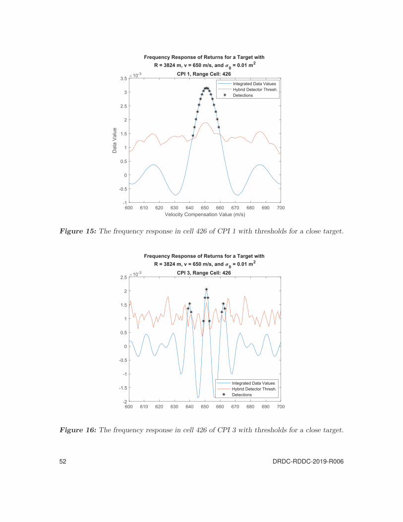
600 610 620 630 640 650 660 670 680 690 700Velocity Compensation Value (m/s)
-1
-0.5
0
0.5
1
1.5
2
2.5
3
3.5
Dat
a V
alue
10-3
Frequency Response of Returns for a Target with R = 3824 m, v = 650 m/s, and 0 = 0.01 m2
CPI 1, Range Cell: 426
Integrated Data ValuesHybrid Detector Thresh.Detections
Figure 15: The frequency response in cell 426 of CPI 1 with thresholds for a close target.
600 610 620 630 640 650 660 670 680 690 700-2
-1.5
-1
-0.5
0
0.5
1
1.5
2
2.5 10-3
Frequency Response of Returns for a Target with R = 3824 m, v = 650 m/s, and 0 = 0.01 m2
CPI 3, Range Cell: 426
Integrated Data ValuesHybrid Detector Thresh.Detections
Figure 16: The frequency response in cell 426 of CPI 3 with thresholds for a close target.
52 DRDC-RDDC-2019-R006

the highest sidelobes. The downside, of course, is that much of the range is now masked toother targets. Compare this with Figure 18, where the same target is located at a distance of8927 m from the radar. Here the sidelobes are already small enough to be indistinguishablefrom noise, so other targets (sufficiently far from the current target) would not be maskedby the pseudo-CFAR detector. In simulations with targets further than 8927, the detectionbehaviour was similar (see below).
Figure 17: The detector response to cross-correlations for a target at 3824 m.
The reason such a large multiple is needed is due to the occasional pathological cross-correlation having a large spike. Figure 19 shows the range returns in which a cross-correlation sidelobe has yielded a spurious detection. The target itself has a distance of6371 m and a speed of 650 m/s, but the figure shows the range returns for the secondCPI in the the neighbourhood of 1000 m, at a frequency compensation value of 578 m/s(a second similar spike was recorded at the same range for 577 m/s). Here, the hybrid de-tector has not detected that sidelobes are present, and so uses the NP threshold. However,a pathological spike in the cross-correlations crosses the threshold. Had the pseudo-CFARdetector been used, the large mutliple would have yielded a threshold much higher thanthe spike, but note that the spike is more than three times larger than nearby sidelobes, sothe multiple for any pseudo-CFAR detector will not only have to be larger than unity, butlarger than unity by a fair margin. When M ≥ 3, these spikes do not lead to the declarationof a “true” target detection unless there is a nearby false alarm in another CPI, althoughit does therefore degrade the actual probability of false alarm; when M < 3 however, eachsuch spurious detection is declared to be a due to a target and so it is imperative thatthey occur no more frequently than the specified probability of false alarm allows for. Thus
DRDC-RDDC-2019-R006 53
0 200 400 600 800 1000Range Cell Number
0
0.5
1
1.5
2
2.5
3
3.5
Dat
a V
alue
10-3
Selected Range Data for a Target withR = 3824 m, v = 650 m/s, and = 0.01 m2
Velocity Compensation: 650 m/s
Integrated Data ValuesHybrid Data Thresh.Detections
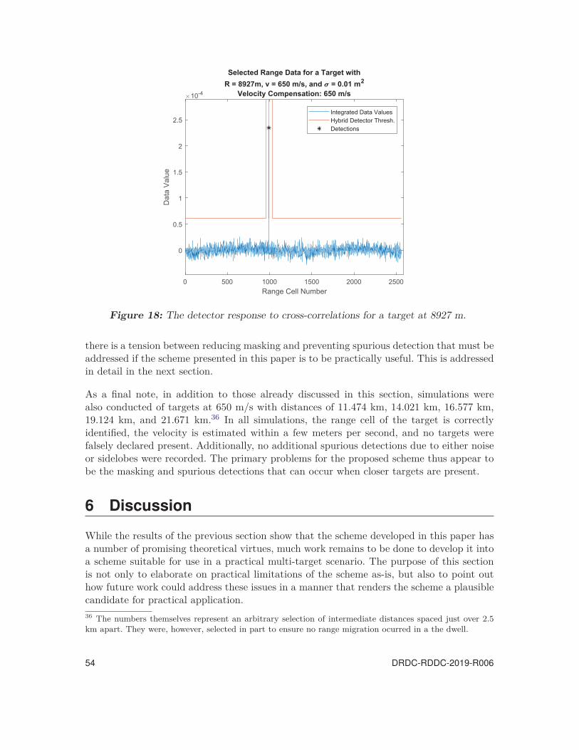
Figure 18: The detector response to cross-correlations for a target at 8927 m.
there is a tension between reducing masking and preventing spurious detection that must beaddressed if the scheme presented in this paper is to be practically useful. This is addressedin detail in the next section.
As a final note, in addition to those already discussed in this section, simulations werealso conducted of targets at 650 m/s with distances of 11.474 km, 14.021 km, 16.577 km,19.124 km, and 21.671 km.36 In all simulations, the range cell of the target is correctlyidentified, the velocity is estimated within a few meters per second, and no targets werefalsely declared present. Additionally, no additional spurious detections due to either noiseor sidelobes were recorded. The primary problems for the proposed scheme thus appear tobe the masking and spurious detections that can occur when closer targets are present.
6 Discussion
While the results of the previous section show that the scheme developed in this paper hasa number of promising theoretical virtues, much work remains to be done to develop it intoa scheme suitable for use in a practical multi-target scenario. The purpose of this sectionis not only to elaborate on practical limitations of the scheme as-is, but also to point outhow future work could address these issues in a manner that renders the scheme a plausiblecandidate for practical application.36 The numbers themselves represent an arbitrary selection of intermediate distances spaced just over 2.5km apart. They were, however, selected in part to ensure no range migration ocurred in a the dwell.
54 DRDC-RDDC-2019-R006
0 500 2000 25001000 1500Range Cell Number
0
0.5
1
1.5
2
2.5
Dat
a V
alue
10-4
Selected Range Data for a Target withR = 8927m, v = 650 m/s, and = 0.01 m2
Velocity Compensation: 650 m/s
Integrated Data ValuesHybrid Detector Thresh.Detections
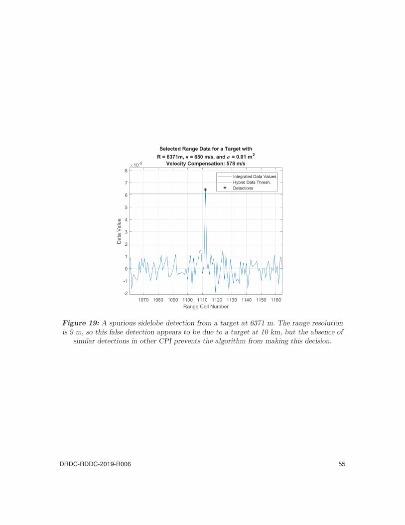
1070 1080 1090 1100 1110 1120 1130 1140 1150 1160Range Cell Number
-2
-1
0
1
2
3
4
5
6
7
8
Dat
a V
alue
10-5
Selected Range Data for a Target withR = 6371m, v = 650 m/s, and = 0.01 m2
Velocity Compensation: 578 m/s
Integrated Data ValuesHybrid Data Thresh.Detections
Figure 19: A spurious sidelobe detection from a target at 6371 m. The range resolutionis 9 m, so this false detection appears to be due to a target at 10 km, but the absence of
similar detections in other CPI prevents the algorithm from making this decision.
DRDC-RDDC-2019-R006 55

6.1 Additional Optimization Constraints
There are number of practical limitations, some of which have been mentioned above, thatare not explicitly included in the optimization problem Eqs. (35a)–(35j), but either are usedimplicitly, or could be included in the problem with neglible change to the structure of theproblem and its solution algorithm:
• Nc ≥ Ncmin . There are two reasons for imposing a minimum Nc value. First, aspreviously discussed, the desired auto- and cross-correlation properties of the phasecodes (Eqs. (4) and (5)) are contingent on them having sufficiently many chips. Second,there must be enough chips for there to be N distinct phase codes, where N is notknown in advance. As an example, one particular experiment (the details are otherwiseunimportant) with the solution algorithm above and Ncmin = 5 yielded N = 31 pulsesper CPI. But there are only 25 = 32 phase codes of length 5, and so a radar usingthese results would run the risk of making false detections due to the repetition ofwaveforms. This constraint does not appear explicitly in the optimization problem,but is used in Algorithm 2 with a value of 10 for all experiments conducted in Section5.
• N ≥ Nmin. This has less operational significance than the lower bound on Nc, anda value of Nmin = 1 does not appear to have any particular issues in principle. Thisconstraint is not explicitly stated in the optimization problem, but is included inAlgorithm 2.
• Nc ≤ Ncmax and N ≤ Nmax. These constraints are in principle necessary only forcomputational purposes. The branch-and-bound algorithm checks “all” pairs (N, Nc),and so needs some finite limit on the total number of such pairs if it is to finish in finitetime. However, a different approach can be taken. For a fixed N one can compute thelargest Nc beyond which no more energy-on-target is needed (for a minimal τc value).So if, for a given N , Ncmin and the smallest τc possible, NNcminτc > Λ by a sufficientlylarge margin, that (N, Nc) pair is putting more energy on target than is needed tosatisfy the constraint Eq. (35f) compared to a (N, Nc) pair with a smaller N , so thebigger N can be pruned. Altough this is not explicitly shown in Algorithm 2, there isan indirect reference to it through the use of Nmax. Proceeding in this fashion rendersreference to Ncmax formally unneccessary: its value is determined indirectly as the Nc
value used when attempting to find a feasible solution with N = 1 and the smallestpossible τc.
• τc ≥ max{c1δ, c2/B}. The parameter δ is defined as the minimum resolution of thecomputer, i.e. the smallest possible difference in τc. We assume for simplicity that thesmallest possible τc is also δ, but it may instead be the case that the minimum samplingrate of the analog-to-digital converter in the radar is much larger, e.g. in [5–9], c1 = 50is used. Similarly, that the chip time can be as small as the inverse of the bandwidthis an at-best condition; a model with more strict spectral cutoff requirements mightuse c2 > 1 to prevent spectral leakage. The good news is that, as seen in Section 5.1,
56 DRDC-RDDC-2019-R006
for large bandwidths, the optimization problem is relatively insensitive to changes inB. Since the form of this constraint is “τc ≥ a constant,” changing the value of theconstant (via c1 or c2) does not change the structure of the problem.
• vmaxN max ti ≤ c3cτc/2. The current range migration constraint only prevents rangemigration from occurring necessarily when targets are travelling at vmax, but saysnothing about how likely it is to occur in other cases. By increasing the value of c3,range migration is made less likely to occur. There may be a way to modify c3 on aprincipled basis, however. The classic mathematical problem of “Buffon’s Needle”37
bears a certain structural similarity to the problem of computing probabilities of rangemigration. “Buffon’s needle” refers to the problem of calculating the probability thata needle of a given length will, when thrown randomly on to the ground, intersectthe boundaries of long rectangular floorboards with a certain fixed separation. Byanalogy, a target travelling at a fixed speed v in the i-th CPI is like a needle of lengthvNti, while the range cells are like the floorboards, and the probability of intersectionis the probability of range migration occurring. In fact, targets undergoing arbitrarymotion can have their probabilities modelled this way: one result related to Buffon’sneedle is that the expected number of intersections of a needle depends only on itslength, but not its shape,38 thus allowing target acceleration and manouevring to bemodelled as well. A brief search of IEEE Xplore for “Buffon’s needle” yields someresults, but, at time of writing, none related to radar range migration, so this maypresent an opportunity for future work to explore.
• rres,min ≤ cτc/2 ≤ rres,max. It may be desirable to place some maximum or minimumcondition on the range resolution of the radar system in use. In particular, limitingthe size of the range resolution may be an important part of limitting the effects ofclutter (by limiting the clutter power per sample) when that is included in the systemmodel in future work. Although no such constraints were considered here (explicitlyor implicitly), the addition of constraints bounding τc does not affect the structureof the problem because there already exist constraints of the same form, just withdifferent values of the constants.
• Pr = . . . /(. . . Ls . . . ). The radar modelled in this paper was ideal in the sense thatit had no losses of any kind in the “back-end.” But a real radar may have mulitplesources of losses, and other practical effects, like attentuation due to atmosphericabsorptivity or phased-array antenna beamforming losses, may be significant enoughto require inclusion in the model. This is easy enough to do by adding terms in thenumerator (for gains) or denominator (for losses) to the ratio under the radical in Eq.(35f), i.e. the term from the radar range equation. This has no effect on the structureof the problem.
• max{ti} ≤ λ/(4vmax). As elaborated on, in Annex A, non-negligible recurrent lobescan appear at multiples of ti, as expressed by the ratio of sinusoids in the ambiguity
37 See, for instance, the Wikipedia page for “Buffon’s Needle,"https://en.wikipedia.org/wiki/Buffon%27s_needle. Accessed 19 October 2018.38 See “Buffon’s Noodle," https://en.wikipedia.org/wiki/Buffon%27s_noodle. Accessed 19 October 2018.
DRDC-RDDC-2019-R006 57
function. This constraint could replace (35d) in order to prevent these lobes fromappearing in the unambiguous range-Doppler map of interest, although it was notnecessary in this paper.
6.2 Real-Time Solution of the Optimization Problem
As mentioned earlier, the length of time taken to complete the algorithm can vary dras-tically: running the solution algorithm for B = 2 MHz and τd,max = 0.1 will take a fewminutes, while a few hours is required for the case when B = 20 MHz and τd,max = 0.4.Now the ideal application for the approach developed in this paper would be as part ofan adaptive (or even cognitive) resource management algorithm that, based on its missionprofile, can specify certain parameters for the optimization problem and then get the re-sulting waveform parameters in real time; an even lofiter goal would involve running theproblem several times for different scenarios and then selected its preferred one in real time(if such comparison could not be facillitated by analysis a priori). This obviously requiresan algorithm capable of running in real time regardless of system parameters, a quality thatcannot be ascribed to the algorithm developed in this paper, even if it were afforded greatercomputational resources than were available at time of writing.
There are two obvious avenues for reducing the computation time: check fewer (M, N, Nc)-tuples, and spend less time checking per tuple. The latter condition explains why reducingthe bandwidth parameter speeds up the algorithm run time, but the former may turn outto be the way to reduce run time in a more systematic way. First, note that, for mostexperiments conducted, all (N, Nc) pairs for M ≥ 5 were pruned, and indeed most forM = 4 were too. So despite the fact that the maximum M checked in the algorithm iscurrently 12, checking 4 ≤ M ≤ Mmax contributes very little to the algorithm run time.The majority of time is spent checking cases when 1 ≤ M ≤ 3. Indeed, even when a feasiblesolution has been found, very few branches in that range of M values are pruned, and so apotentially large number of (N, Nc) pairs (potentially in the thousands to tens of thousands)are checked. It may, however, be possible to obtain a solution with performance close towhat is obtained currently by checking a much smaller number of (N, Nc).
Consider the optimal objective function value of the convex relaxation subproblem in Eqs.(36a)-(36f). If N and Nc have values such that Λ/(NNc) > max{δ, 1/B}, then the solutionfrom Theorem 1 gives τ∗
c = Λ/(NNc) and ti = Ncτ∗c /τd,max for all i, for a total dwell time
of
t∗D =
M∑i=1
N
(Nc
τd,max
( ΛNNc
))−
(Nc
τd,max
( ΛNNc
))+ Nc
( ΛNNc
)+
2Rmax
c
=MΛ
τd,max+
ΛN
(1 − 1
τd,max
)+
2Rmax
c. (60)
Crucially, Eq. (60) does not have Nc appear in the optimal value. For a fixed N (and ifτc is a real variable), then whenever τc is limited below by the energy-on-target constraint
58 DRDC-RDDC-2019-R006

Eq. (35f), change in the value of Nc does not change the value of tD. Specifically, whenthe aforementioned conditions hold, variation in Nc is exactly matched by a change in τc
such that Ncτc is fixed: Ncτ∗c = Nc(Λ/(NNc)) = Λ/N . Now, this doesn’t exactly hold for
Eqs.(35a)-(35j) because τc is an integer multiple of δ, but the insight is still useful, as Nc
only ever appears explicitly in the problem (namely in Eqs. (35a), (35c), and (35f)) in aproduct with τc. Because τc is an integer multiple of δ there are instances where variationNc is not sufficient to warrant a change of τc to the next nearest multiple of δ, so this new(Nc, τc) pair may be strictly larger or smaller than the previous pair. However, satisfactionof other constraints notwithstanding, this change in size is still bounded insofar as δ issmall.
Suppose that, by chance, Ncτc value for a given N and a real τc variable should happento be expressible as the product of an integer and an integer multiple of δ, i.e. so that theNcτc value is achievable in the real problem Eqs. (35a)–(35j). Suppose further that Nc ifincreased by small amounts, this change is not larger enough to warrant a decrease in τc, i.e.(Nc + n)(τc − δ) < Ncτc and thus infeasible. How large can (Nc + n)τc get before τc − δ canfeasibly be used? Recalling that τc = bδ by definition, it is straightforward to show that thecondition (Nc +n)(τc −δ) ≥ Ncτc yields n ≥ Nc/(b−1) as the condition for τc −δ = (b−1)δbeing feasible. This suggests that dwell time as a function of Nc will have a sort of sawtoothshape with an increasing amplitude. Each subsequent Nc value increases the dwell time untilit is large enough for τc to be decreased, and the dwell time drops precipitously (comparing(Nc + n − 1)bδ to (Nc + n)(b − 1)δ gives a drop of Nc + n − b).39 When the pulse lengthdecreases, the PRIs can decrease via the maximum duty cycle constraint Eq. REF, so thedwell time as a whole is reduced.
The significant message is this: although for a given N there may be only one minimizing(Nc, τc) pair, there are likely many such pairs that yield very close values. How the twovariables are related in the full problem has been explored above, and with further work, itmay be possible to develop a method that checks only a small number of Nc values per N- perhaps only one.
Is a similar argument possible for N itself? While Eq. (60) does suggest a small N , this maybe somewhat misleading. This equation was used to characterize variation in Nc and τc fora fixed N , but by varying over N as well, the net variation in the dwell time becomes lesspredictable: the objective function Eq. (36a) explicitly decreases in N , but as N decreases,Ncτc must increase, so the ti variables increase, and the net effect on the product Nti isunclear. Nevertheless, there is still good reason to believe in the possibility of checking onlya small number of N values before settling on a solution that yields results close to the onespresented in this paper.
In Section 5.1, much discussion referred to changes in the value of NNcτc without regardto the individual values of the variables themselves. Indeed, in the discussion of Figure39 To see that this is positive, note that n is defined as the smallest integer such that (Nc +n)(τc −δ) ≥ Ncτc
holds. Working through the algebra, this yields an equivalent condition: nb ≥ Nc + n. For larger Nc, n > 1,so b < Nc + n.
DRDC-RDDC-2019-R006 59
(7) and Table 3 it was noted that despite large changes in bandwidth (and thus τc), thetotal dwell time remained approximately constant because variation in N and Nc keptNNcτc approximately constant. It thus seems plausible that a large number of (N, Nc, τc)-tuples (namely those with a value approximately equal to Λ) result in approximately similardwell times. This in turn means that one may be able to choose their values with relativefreedom, provided the other constraints are met. Using the insights developed in this paper,an efficient but high-performing algorithm could thus have the following heuristic form:
1. Based on the nominal visibility parameter and the insight of Figures 5 and 8, selectan appropriate M (e.g. M = 1 for lower visibility, M = 3 for high visibility).
2. Select a desirable N .
3. Having computed Λ, compute the necessary Ncτc required for τc ∈ R (the resultingvalue of Ncτc may influence which N values are desirable).
4. Using the analysis in this section, choose good values for Nc and τc based both onhow close the resulting product is to the minimum Ncτc, but also potentially on otherdesiderata.
5. With (N, Nc, τc) specified, Eq. (35c) can be used to compute the minimum allowableti, while Eq. (35g) can be used to calculate the maximum allowable ti. With a set ofti values maximally spread out in that interval, satsifaction of the visibility constraintcan be determined. If it satsified, shrink the spacing of the ti down unitl just beforeit isn’t, otherwise, a new (N, Nc, τc) set will be required (further providing conditionson what desireable N and Nc values look like).
Further work is required to develop not only the algorithm described above, but also tobetter understand the relevant insights and desiderata on which it is based. For instance,Eq. (35g) suggests a smaller N for a larger maximum ti, while a larger Nc may be desirableto reduce the size of the waveform sidelobes. And with sufficient study, it may be possible todevelop the algorithm to the point where, reliably, only one (M, N, Nc, τc) is checked, dras-tically reducing the algorithm time compared to the one in this paper, without significantloss of performance.
Thus this appears to be a promising line of future research. While such an algorithm wouldbe desirable for its efficiency alone, the next section highlights how the freedom to choosecertain parameters could provide another significant improvement over and above the de-velopments of this paper.
6.3 Masking and Other Waveform Considerations
At the outset of this paper, it was assumed that there were a set of almost arbitrarily manycodes of nearly any length that had a delta-like autocorrelation and a near-vanishing cross-correlation between any two codes. As the paper progressed, practical limitations to suchan assumption became readily apparent. The chaotic phase codes had typical peak sidelobe
60 DRDC-RDDC-2019-R006

levels in the range of -26 dB to -32 dB, which may still be too high for practical applica-tion; while the simulations for targets at medium and large distances showed the schemeworking as desired, the presence of close targets resulted in severe masking throughout theunambiguous range and spurious detections of sidelobes, which, though rare, was not asrare as the desired PF A required it to be. In this section, future research directions thatseek to mitigate these issues are addressed.
The first point to be made has already been stated earlier in the text. Because only singletargets were under consideration in this work, the pseudo-CFAR detector had the formof a product between some constant and the largest value in the test window. By usingthe k-th largest value instead, up to k − 1 targets could potentially be identified in closeproximity. But this does not address the issues with pathological cross-correlations. A moregeneral approach to both masking and these cross-correlations is to use better waveforms.Two points must be made to this end. First, the logistic phase codes used here sufficed toillustrate a proof-of-concept, but other more promising approaches do exist. As discussedin Section 4.1, the development of chaotic phase codes with more suitable sidelobe levelsis an active area of research, with some promising candidates for real-time generation ofwaves already available in [84,85,94]. The second point relates to the choice of chaotic phasecodes in the first place. They were chosen for their capacity to generate distinct waves in realtime without knwoing in advance how many would be required. But there is an alternative.Only a compartively small number of waves are ever in the air at the same time: for theparameters in Table 1 (i.e. the solution in Table 4), 145*3 = 435 codes are needed, butbecause the unambigous range round trip time is 2Rmax/c = 0.1533ms and, for example,the PRI in the first CPI is 12 μs, the number of waves in the air at any one time is givenby �153.33/12� = 12. Thus a given wave only needs to have a good cross-correlation withthe 12 waves in front of and behind it.40 And while this number is not known in advance,it is much smaller than “arbitrarily many,” so the prospect of developing a library of usefulwaves in advance (as opposed to generating them in real time) becomes more plausible.
Moreover, since there appears to be some flexibility in the choice of N (Section 6.2), andan additional constraint could be added to the optimization problem without affecting itsstructure or results drastically: add min{ti} ≥ 4Rmax/(cNunique)), where Nunique is themaximum number of pulses compatible pulses available.41 This is a convex constraint (andequivalent to M linear constraints of the form ti ≥ 4Rmax/(cNunique) and so does notmake the optimization problem much harder in general, but if Nunique is large enough that40 In contrast to the strategies discussed below, a more real-time-oriented approach would be to computethe number of waves in the air at any one time (say, 12) before running the system, and then checking eachnew phase code for compatibility with the previous 12. If it is incompatible, e.g. generates a spike of unduesize, search for another phase code, and so on. The drawback is that this process takes an unknown lengthof time, but for large enough Nc it is unlikely to take long.41 This constraint forces ti to be large enough so that the maximum number of required compatible wavesnever exceeds 2Nunique. To see this note that the number of pulses in the air at any during CPI i is given by�2Rmax/(cti)�; the transitions between CPI is more complex, but this expression can be maximized acrosstimes by using min{ti} instead of ti. Thus 2�2Rmax/(c min{ti})� ≤ Nunique is the “true” constraint. Butthis is not convex, so, noting that �x� ≤ x, we remove the floor function (and rearrange variables) to obtainthe slightly more stringent, but convex, constraint listed above.
DRDC-RDDC-2019-R006 61

4Rmax/(cNunique) ≤ Ncmin max{δ, 1/B}, then this new constraint can never be active, andthus literally does not change the structure of the problem at all.
At this point it is fair to compare the concern here as being essentially similar to waveformdesign in MIMO radar (see also the discussion and references in Section 4.1). One broadstrategy for MIMO radar is to have one waveform for each antenna, such that each waveformhas a delta-like autocorrelation and the set of waveforms has pairwise near-zero cross-correlation. If, as discussed above, the number of waveforms of the scheme in this paper canbe fixed in advance, then the problem of finding suitable waveforms is equivalent to the sameproblem for a MIMO radar with a fixed number of antennas.42 Thus future work related tothis paper should be able to leverage the large volume of literature related to MIMO radar.However, given the results of Section 6.2, we may have an additional advantage.
If the efficient approach of Section 6.2 is fleshed out, and it turns out that N can indeedbe chosen (more or less) arbitrarily, then one approach to choosing N could simply be toselect N to be number of waveforms in some fixed-number-of-waveform approach discussedin Section 1.2.2,. These were originally dismissed (in part) for not being amenable to op-timization because either N is fixed, or there are multiple possible N values but not onefor each positive integer. But if N is now (more or less) free, that possibility is open again.Consider, for example, the Ipatov code-based approach of [48]. This uses N pulses mod-ulated by a length-N Ipatov code, which have a perfect correlation response when usingthe appropriate mis-matched filter, i.e. there are, in theory, no sidelobes at all. This wouldcompletely eliminate issues related to both the pathological cross-correlations and masking.Other approaches may not offer nominally perfect correlations, but would likewise offersubstantial improvement.
To summarize, although masking of and pathological cross-correlations by close targetspresent an obstacle to practical use for the scheme in this paper, there exist promisingavenues of future research that could mitigate these effects. The outcome of research in Sec-tion 6.2 notwithstanding, the possibility of using a relatively small number of pre-computedcompatible waves, whether chaotic phase codes, MIMO radar waves, or otherwise, is plausi-ble. Moreover, if the research in Section 6.2 does indeed prove fruitful, further improvement(potentially up to and including the complete elimination of sidelobes) could be had byincorporating one of the schemes discussed in Section 1.2.2.42 Of course, another broad strategy for MIMO radar is to transmit waves on orthognal frequency bandsto gain the necessary “separation” between different waves, an idea that has been otherwise ignored here.Given that our scheme is tolerant to large variations in bandwidth, a multiple-frequency strategy may infact be prudent. For example, if 6 MHz of bandwidth is available, then since the scheme does just as well atwith 2 MHz of bandwidth, further speed gains could be obtained by transmitting each CPI on separate 2MHz sections of bandwidth. The question of optimality in this case would of course need to be addressed bya separate optimization problem, which is beyond the scope of this work, but may be a profitable directionfor future work.
62 DRDC-RDDC-2019-R006
6.4 Clutter
Although it is not a subject of focus in this paper, several references to clutter and themitigation of its effects have been made throughout, as any practically useful version of thisscheme must be capable of tolerating those effects. In particular, it has been noted thatimposing an upper limit on the size of a range cell would limit the amount reflected powerdue to clutter in each cell, while the use of a (non-hybrid) CFAR detector is undoubtedly anecessity in a practical scenario. The primary difficulties to this end will be first, determininghow to maintain the desired performance guarantees (i.e. in terms of PF AO
and PDO) with
the new, less mathematically transparent CFAR structure,43 and second, determining howto reflect this change in the optimization problem. Possibilities for this latter goal range fromthe simple (and structure preserving), like including a constant “CFAR loss” term (see [2],pp. 601–603) in the denominator of the SNR expression in Eq. (35f), to the complicated(and structure modifying), like replacing Eq. (35f) entirely with the (likely nonconvex)expressions for the probabilities of false alarm and detection of the given CFAR detectorstructure. Other practical issues will follow, like the modification of the visibility mapconstraint Eq. (35e) to include the velocity dimension in addition to the range dimension.Compared to the previous few sections in Section 6, this has not been explored in muchdepth, but the practical necessity of it demands further research.
6.5 Other Practical Considerations
Here we discuss at varying lengths different practical considerations not covered by theabove, presented in no particular order.
• First, some notes on “visibility” as used in this paper. The value of ζ is often referredto as “nominal” visibility, because there are a few qualifications that prevent it frombeing the “true” visibility, whatever that should turn out to mean. First, although arange cell may be nominally visible, it may still be the case that a target is harderto detect there than in some other nominally visible cell of comparable distance.Consider a target close to a series of eclipsed cells. If several of the chips in the phasecode returned from the target are eclipsed, the peak of the autocorrelation will notbe as high as it would have been had all chips remained uneclipsed. A more completecharacterization of visibility would include this kind of distinction, i.e. the differencebetween visible, eclipsed, and partially visible. As a related example, [9] notes thedifference between range/Doppler cells which are visible in the minimum number ofCPI and in more than the minimum number of CPI. They also model the time ittakes for the radar to switch from transmission to reception, something which is notconsidered here. Finally, more work must be done to characterize the effect of theparameter κ. The value used in this paper (κ = 0.8) was chosen heuristically. It seemspossible, however, that by increasing κ, less energy-on-target is required and thusdwell time could be reduced; on the other hand, increasing κ reduces visibility andthus could result in increased dwell time by forcing larger PRI values.
43 An alternative and less optimistic approach is to instead determine what gurantees, if any, can be made.
DRDC-RDDC-2019-R006 63

• The frequency compensation method used in this paper was adopted heuristically,and other choices could exist. Indeed, given the frequency artefacts that result inlater CPI, alternative method may be prefereable. This is, however, a less urgent needthan other concerns discussed in this paper: masking in the frequency domain onlyoccurs to targets with nearby frequencies and the same range bin, whereas the rangedomain masking of the pseudo-CFAR detector poses a more serious problem.
• On the topic of frequency compensation, more work needs to be done to characterizethe Doppler tolerance of whatever waveforms are ultimately used (whether the chaoticphase codes of this paper or some other kind as per Section 6.3). While the frequencycompensation method used in this paper is amenable to parallelization, if too manyparallel computations are required, it may still be infeasible. The velocity resolutionused in all simulations here was 2 m/s (at a frequency of 3 GHz), which for an unam-biguous velocity of ±700 m/s, entails 701 different values for frequency compensation(rounding up). If the waveforms ultimately used can tolerate an even greater sepa-ration, then that value could drop even further, making real-time operation all themore feasible.
• Eq. (1) describes the upper bound on the product of the unambiguous range andvelocity for ordinary radar operation: Rmaxvmax ≤ cλ/8. The technique presented inthis paper was implemented for Rmax = 23 km and vmax = 700 m/s, whose respectivecounterparts from Eq. (1) are vmax ≈ 163 m/s and Rmax ≈ 5.36 km, and so the newtechnique (in this case) yielded an improvement by a factor of approximately 4.3.But no statement about the general capability of the scheme has yet given, so here weattempt to derive a bound similar to that of Eq. (1) (but in a more qualified sense) forthis scheme to explore what unambiguous range and velocity pairs are theoreticallypossible. As range increases, the NNcτc value required increases, and for maximumrange, they will each need to be at their largest. Now τc = λ/(4vmax) is the largestpossible chip time (Eq. (35d)), which in turn places bounds on the other variables asN = cτc/(2vmax max{ti}) (Eq. (35g)) and Nc = (τd,max/τc) min{ti} (Eq. (35c)). Thisyields
NNcτc =(
cτc
2vmax max{ti}) (
τd,max
τcmin{ti}
) (λ
4vmax
)
=(
cλτd,max
8v2max
) min{ti}max{ti} (61)
≤ cλτd,max
8v2max
(62)
Now if M = 1, then min{ti} = max{ti} exactly, but even for other M , the values ofthe PRI are going to be large and the variation in ti comparitively small (althoughthis depends on ζ), so the bound in Eq. (62) is not strictly tight but could be very
64 DRDC-RDDC-2019-R006
close. Then, rearranging Eq. (35f), we get
(Q−1(PF A) − Q−1(PD)
)2 ≤ 2PtGtGtλ2σ0NNcτc
(4π)3R4maxkT0F
≤ 2PtGtGtλ2σ0
(4π)3R4maxkT0F
(cλτd,max
8v2max
)
Which is then rearranged to obtain the bound
R2maxvmax ≤
√2PtGtGtλ3σ0cτd,max
(8π)3(Q−1(PF A) − Q−1(PD))2kT0F. (63)
Some qualification is required, however. First, note that is depends on PF A and PD.The bound must therefore be evaluated with respect to a single M value; for a givenset of radar system parameters, the full bound will be given by the minimum amongthe individual bounds for all plausible M . Because τc is known, the number of rangecells is known, and so PD and PF A can be computed exactly. For low ζ values, i.e.such that M = 1 is optimal, this bound is thus tight. For other M (as previouslymentioned), min{ti} < max{ti} but it will also be the case that min{ti}/ max{ti} ≈ 1,so the bound will not be tight but will not be far off. Most important, however, isthis: Eq. (63) represents the mathematical possibility of finding a feasible point in theoptimization problem Eq. (35a)–(35j). Even if a feasible solution is found for at, say,Rmax = 100 km and vmax = 3000 m/s, the resulting dwell time may be prohibitivelylarge. So, in a loose sense, Eq. (63) bounds what is “possible” for the scheme presentedin this paper, but not necessarily what is useful or practical.Figure 20 compares this bound for the parameters of Table 1 to the baseline bound ofEq. (1) at the same wavelength. This new bound (calculated with respect to M = 3for the default parameters) improves upon the old one by as much as two ordersof magnitude in some instances. Crucially, this improvement can be increased bychanging aspects of the radar itself, e.g. increasing transmission power, antenna gain,etc., and is not just a fixed amount.
7 Summary
The disambiguation of pulse-Doppler radar range and velocity measurements is a problemthat has garnered attention for decades, and in military contexts, the motivation is obvious:detecting faster hostile targets from further away provides more time to prepare an adequateresponse. And yet very little attention has been paid in the literature to two importantconsiderations: first, the dwell time required to perform the necessary measurments, andsecond, the detection performance of the radar under the new unambigusous range/Doppler.These concerns notwithstanding, common approaches to disambiguation have additionalproblems: approaches using multiple PRFs have ghosts and result in a coupling of theachievable unambiguous range and Doppler, while approaches using waveform diversity
DRDC-RDDC-2019-R006 65

often struggle with eclipsing of potential target returns, and few approaches of either kindare amenable to the kind of variation in parameter values that is necessary to permitoptimization over those values.
The disambiguation scheme presented in this paper addresses these shortcomings by using ajoint multiple-PRF/diverse waveform approach. A greater unambiguous range is achieved byusing distinct phase-coded waveforms with delta-like autocorrelations (for good detectionperformance) and near-zero cross-correlation (to prevent spurious detection). A greaterunambiguous velocity is achieved using a frequency compensation method that exploits therelatively small chip times of the phase codes rather than relative large pulse repetitionintervals. The fact that the function of the scheme is not dependent on the specific values ofits parameters allows those parameters to be optimized with respect to the minimization ofdwell time. The constraints of this optimization problem ensure, among other things, certainnominal visiblity, a fixed overall probability of false alarm, and a minimum probability ofdetection for all targets in the unambiguous range.
This optimization problem was studied and found to have a hidden convex character. Indeed,the study and exact characterization of two convex subproblems formed the basis of thebranch-and-bound algorithm used to solve the original problem. This solution algorithmwas then used to study how the performance of the scheme (in terms of dwell time) isimpacted by variation in different system parameters. It was found that while increasedradar “quality” and duty cycle can help reduce dwell time, increasing the nominal visibilityrequires a greater dwell time. The scheme was also noted for its relative insensitivity to largevariation in bandwidth: even though the minimum chip time changes drastically, variationin the number of chips per pulse and the number of pulses copmensates with little changein overall performance.
The performance of the scheme itself was also studied via simulation. As advertised, thescheme can detect a minimally-sized target at the maximum range and speed, and handlesmedium- and long-distance targets well. However, when dealing with targets close to theradar, the non-ideal performance of the chaotic phase codes resulted in behaviour thathas the potential to mask other legitimate targets and result in spurious false alarms.While this behaviour would prevent the scheme from being practically viable in its currentform, a number of research avenues have been identified that could make the scheme viablein the future. In particular, the bandwidth insensitivity property described above mayprovide a path to the development of a time-efficient solution algorithm that achieves aperformance nearly as good as the one presented in this paper. By allowing the almostarbitrary selection of certain waveform parameters, this new algorithm would allow the useof high-quality waveforms, like those used in MIMO radar or in other waveform diversedisambiguation schemes, could completely mitigate the pathologies of the current system.With the theoretical groundwork laid, and future avenues of research identified, the workpresented in this paper provides a plasuible basis for a practical approach to disambiguation.
66 DRDC-RDDC-2019-R006
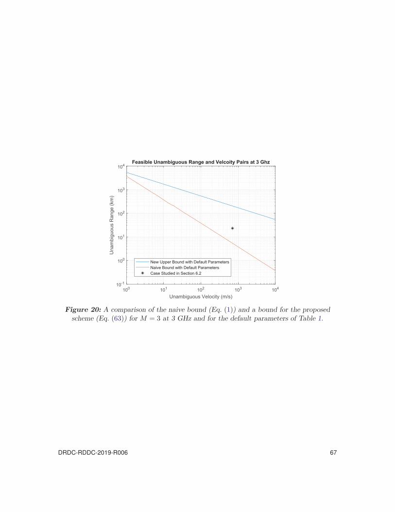
100 101 102 103 104
Unambiguous Velocity (m/s)
10-1
100
101
102
103
104
Una
mbi
guou
s R
ange
(km
)
Feasible Unambiguous Range and Velcoity Pairs at 3 Ghz
New Upper Bound with Default ParametersNaive Bound with Default ParametersCase Studied in Section 6.2
Figure 20: A comparison of the naive bound (Eq. (1)) and a bound for the proposedscheme (Eq. (63)) for M = 3 at 3 GHz and for the default parameters of Table 1.
DRDC-RDDC-2019-R006 67

References
[1] Proakis, J. G. and Manolakis, D. G. (2007), Digital Signal Processing (4th Ed.):Principles, Algorithms, and Applications, Upper Saddle River, NJ, USA:Prentice-Hall, Inc.
[2] Richards, M. A., (Ed.) (2010), Principles of Modern Radar: Basic Principles, Radar,Sonar, and Navigation, Institution of Engineering and Technology.
[3] Moo, P. and Ding, Z. (2016), Adaptive Radar Resource Management, ElsevierScience and Technology Books.
[4] Dummit, D. and Foote, R. (2004), Abstract Algebra (3rd Ed.), Wiley.
[5] Davies, P. G. and Hughes, E. J. (2002), Medium PRF set selection using evolutionaryalgorithms, IEEE Transactions on Aerospace and Electronic Systems, 38(3), pp.933–939.
[6] Hughes, E. J. and Alabaster, C. M. (2003), Medium PRF radar PRF optimisationusing evolutionary algorithms, IEEE Radar Conference, pp. 192–197.
[7] Hughes, E. J. and Alabaster, C. M. (2003), Novel PRF schedules for medium PRFradar, IEEE International Conference on Radar, pp. 678–683.
[8] Alabaster, C. M., Hughes, E. J., and Matthew, J. H. (2003), Medium PRF radarPRF selection using evolutionary algorithms, IEEE Transactions on Aerospace andElectronic Systems, 39(3), pp. 990–1001.
[9] Wiley, D., Parry, S., Alabaster, C., and Hughes, E. (2006), Performance comparisonof PRF schedules for medium PRF radar, IEEE Transactions on Aerospace andElectronic Systems, 42(2), pp. 601–611.
[10] Thomas, A. G. and Berg, M. C. (1994), Medium PRF set selection: an approachthrough combinatorics, IEE Proceedings - Radar, Sonar and Navigation, 141(6), pp.307–311.
[11] Ahn, S., Lee, H., and Jung, B. (2011), Medium PRF set selection for pulsed Dopplerradars using simulated annealing, IEEE Radar Conference, pp. 90–94.
[12] Kenyon, C. M. and Goodman, N. A. (2010), Range-Doppler ambiguity mitigation viaclosed-loop, adaptive PRF selection, International Conference on Electromagnetics inAdvanced Applications, pp. 608–611.
[13] Rihaczek, A. W. (1973), A systematic approach to blind-speed elimination, IEEETransactions on Aerospace and Electronic Systems, 9(6), pp. 940–947.
[14] Rihaczek, A. W. (1973), Choice of burst number for blind-speed avoidance, IEEETransactions on Aerospace and Electronic Systems, 9(5), pp. 778–781.
68 DRDC-RDDC-2019-R006
[15] Trunk, G. and Brockett, S. (1993), Range and velocity ambiguity resolution, IEEENational Radar Conference, pp. 146–149.
[16] Trunk, G. V. and Kim, M. W. (1994), Ambiguity resolution of multiple targets usingpulse-Doppler waveforms, IEEE Transactions on Aerospace and Electronic Systems,30(4), pp. 1130–1137.
[17] Tuinstra, T. R. (2016), Range and velocity disambiguation in medium PRF radarwith the DBSCAN clustering algorithm, IEEE National Aerospace and ElectronicsConference and Ohio Innovation Summit, pp. 396–400.
[18] Li, X., Xia, X. G., and Liang, H. (2010), A robust Chinese remainder theorem withits applications in moving target Doppler estimation, IEEE Radar Conference,pp. 1289–1294.
[19] Zhen-xing, H. and Zheng, W. (1987), Range ambiguity resolution in multiple PRFpulse Doppler radars, IEEE International Conference on Acoustics, Speech, andSignal Processing, pp. pp. 1786–1789.
[20] Crouse, D. (2014), Maximum likelihood postdetection radar ambiguity resolution,IEEE Transactions on Aerospace and Electronic Systems, 50(3), pp. 1876–1883.
[21] Cai, F., Fan, H., Lu, Z., and Fu, Q. (2015), Bernoulli filter for range and Dopplerambiguous radar, IET Signal Processing, 9(9), pp. 647–654.
[22] Gerlach, K. and Andrews, G. A. (1990), Cascaded detector for multiple high-PRFpulse Doppler radars, IEEE Transactions on Aerospace and Electronic Systems,26(5), pp. 754–767.
[23] Ferrari, A., Bérenguer, C., and Alengrin, G. (1997), Doppler ambiguity resolutionusing multiple PRF, IEEE Transactions on Aerospace and Electronic Systems, 33(3),pp. 738–751.
[24] Xia, X.-G. (1999), Doppler ambiguity resolution using optimal multiple pulserepetition frequencies, IEEE Transactions on Aerospace and Electronic Systems,35(1), pp. 371–379.
[25] Hovanessian, S. A. (1976), An algorithm for calculation of range in a multiple PRFradar, IEEE Transactions on Aerospace and Electronic Systems, 12(2), pp. 287–290.
[26] Immediata, S., Petrucci, R., Timmoneri, L., and Vigilante, D. (2008), New approachto 2D medium PRF ambiguity resolution with application to air surveillance radar,IEEE Radar Conference, pp. 1–4.
[27] Militiev, R. and Arnaudov, R. (2004), Adaptive algorithm for Doppler ambiguityresolution in multiple target situations, IEEE International Conference on IntelligentSystems, 3, pp. 98–101.
DRDC-RDDC-2019-R006 69
[28] Lei, W., Long, T., and Han, Y. (2000), Resolution of range and velocity ambiguity fora medium pulse Doppler radar, IEEE International Radar Conference, pp. 560–564.
[29] Reddy, N. and Swamy, M. (1984), Resolution of range and Doppler ambiguities inmedium PRF radars in multiple-target environment, IEEE International Conferenceon Acoustics, Speech, and Signal Processing, pp. 514–517.
[30] Li, Y., Xu, C., Yan, X., and Liu, Q. (2017), An improved algorithm for Dopplerambiguity resolution using multiple pulse repetition frequencies, InternationalConference on Wireless Communications and Signal Processing, pp. 1–5.
[31] Sun, J., Tian, J., Wang, G., and Mao, S. (2010), Doppler ambiguity resolution formultiple PRF radar using iterative adaptive approach, Electronics Letters, 46(23),pp. 1562–1563.
[32] Bérenguer, C. and Alengrin, G. (1996), Performance indicators of the correlationprocess for non ambiguous doppler frequency estimation in multiple PRF radars,European Signal Processing Conference, pp. 1–4.
[33] van Genderen, P. and Meijer, W. J. H. (1995), Non coherent integration in a mediumPRF radar, IEEE International Radar Conference, pp. 91–94.
[34] Wang, C. J. and Wu, C. H. (1993), Analog neural networks solve ambiguity problemsin medium PRF radar systems, IEEE International Conference on Neural Networks,pp. 120–125.
[35] Long, W. H. and Harriger, K. A. (1985), Medium PRF for the AN/APG-66 radar,Proceedings of the IEEE, 73(2), pp. 301–311.
[36] Nagel, D. and Hommel, H. (2001), A new HPRF mode with highly accurate rangingcapability for future airborne radars, CIE International Conference on Radar,pp. 275–280.
[37] Anderson, J. M., Temple, M. A., Brown, W. M., and Crossley, B. L. (2001), Anonlinear suppression technique for range ambiguity resolution in pulse Dopplerradars, IEEE Radar Conference, pp. 141–146.
[38] Kurian, J., Temple, M. A., Papaphotis, M. J., and Brown, W. M. (2003), Mutuallydispersive pulse coding to enhance non-linear ambiguity suppression, IEEEInternational Conference on Radar, pp. 694–699.
[39] Jenshak, J. D. and Stiles, J. M. (2009), Transmit coding with a range ambiguity,International Waveform Diversity and Design Conference, pp. 98–102.
[40] Omar, S. M., Kassem, F., Mitri, R., Hijazi, H., and Saleh, M. (2015), A novel barkercode algorithm for resolving range ambiguity in high PRF radars, European RadarConference, pp. 81–84.
70 DRDC-RDDC-2019-R006
[41] Lin, F. and Steiner, M. (2001), New techniques for radar coherent range ambiguityresolution, IEEE Radar Conference, pp. 99–104.
[42] Keel, B. M., Baden, J. M., and Heath, T. H. (2007), A comprehensive review ofquasi-orthogonal waveforms, IEEE Radar Conference, pp. 122–127.
[43] Hu, J., Lu, D., Liao, Z., Liu, S., and Zhang, J. (2016), Range ambiguity resolution forhigh PRF radar with random frequency hopping waveforms, IEEE InternationalConference on Digital Signal Processing, pp. 70–73.
[44] Feixing, W., Yongfeng, Z., Hongzhong, Z., and Qiang, F. (2006), Method of resolvingthe range ambiguity for high PRF stepped-frequency radar, CIE InternationalConference on Radar, pp. 1–4.
[45] Chen, Y., Peng, W., Wu, Q., Hao, W., and Liu, C. (2010), A novel method ofresolving velocity ambiguity in the pulse doppler radar, International Congress onImage and Signal Processing, pp. 4321–4323.
[46] Tigrek, R. F., Heij, W. J. A. D., and Genderen, P. V. (2012), OFDM signals as theradar waveform to solve doppler ambiguity, IEEE Transactions on Aerospace andElectronic Systems, 48(1), pp. 130–143.
[47] Duan, J., He, Z., and Han, C. (2006), A novel doppler radar using only two pulses,CIE International Conference on Radar, pp. 1–4.
[48] Levanon, N. (2009), Mitigating range ambiguity in high PRF Radar using inter-pulsebinary coding, IEEE Transactions on Aerospace and Electronic Systems, 45(2), pp.687–697.
[49] Rouffet, T., Grivel, E., Vallet, P., Enderli, C., and Kemkemian, S. (2015), Combiningtwo phase codes to extend the radar unambiguous range and get a trade-off in termsof performance for any clutter, In IEEE International Conference on Acoustics,Speech and Signal Processing, pp. 1822–1826.
[50] Akhtar, J. (2009), Cancellation of range ambiguities with block coding techniques,IEEE Radar Conference, pp. 1–6.
[51] Zhu, J., Zhao, T., Huang, T., and Zhang, D. (2016), Analysis of random pulserepetition interval radar, IEEE Radar Conference, pp. 1–5.
[52] Rasool, S. B. and Bell, M. R. (2010), Efficient pulse-Doppler processing andambiguity functions of nonuniform coherent pulse trains, IEEE Radar Conference,pp. 1150–1155.
[53] Duan, J. Q., He, Z. S., and Qin, L. (2008), A new approach for simultaneous rangemeasurement and Doppler estimation, IEEE Geoscience and Remote Sensing Letters,5(3), pp. 492–496.
DRDC-RDDC-2019-R006 71

[54] Deng, H., Himed, B., and Wicks, M. C. (2007), Concurrent extraction of target rangeand doppler information by using orthogonal coding waveforms, IEEE Transactionson Signal Processing, 55(7), pp. 3294–3301.
[55] Jang, D. S. and Choi, H. L. (2012), Heuristic pulse interleaving algorithms formulti-target tracking on pulse Doppler phased array radars, IEEE Radar Conference,pp. 558–563.
[56] Zhang, Y., Deng, Z., Shi, J., Ye, L., Fu, M., and Zhao, C. (2015), Doppler ambiguityresolution based on random sparse probing pulses, Journal of Electrical andComputer Engineering.
[57] Quan, Y. H., Zhang, L., Xing, M. D., and Bao, Z. (2011), Velocity ambiguityresolving for moving target indication by compressed sensing, Electronics Letters,47(22), pp. 1249–1251.
[58] Shaban, F. and Richards, M. A. (2013), Application of L1 reconstruction of sparsesignals to ambiguity resolution in radar, IEEE Radar Conference, pp. 1–6.
[59] Sachidananda, M. and Zrnic, D. S. (1999), Systematic phase codes for resolving rangeoverlaid signals in a doppler weather radar, Journal of Atmospheric and OceanicTechnology, 16(10), pp. 1351–1363.
[60] Sachidananda, M. and Zrnic, D. S. (2003), Unambiguous range extension by overlayresolution in staggered PRT technique, Journal of Atmospheric and OceanicTechnology, 20(5), pp. 673–684.
[61] Bharadwaj, N. and Chandrasekar, V. (2007), Phase coding for range ambiguitymitigation in dual-polarized doppler weather radars, Journal of Atmospheric andOceanic Technology, 24(8), pp. 1351–1363.
[62] Ruzanski, E., Hubbert, J. C., and Chandrasekar, V. (2008), Evaluation of thesimultaneous multiple pulse repetition frequency algorithm for weather radar,Journal of Atmospheric and Oceanic Technology, 25(7), pp. 1166–1181.
[63] Paepolshiri, N., Pace, P. E., and Jenn, D. C. (2012), Extending the unambiguousrange of polyphase P4 CW radar using the robust symmetrical number system, IETRadar, Sonar Navigation, 6(7), pp. 659–667.
[64] Kronauge, M., Schroeder, C., and Rohling, H. (2010), Radar target detection andDoppler ambiguity resolution, International Radar Symposium, pp. 1–4.
[65] Aittomäki, T. and Koivunen, V. (2012), Target velocity estimation with distributedMIMO radar using multiple pulse repetition frequencies, IEEE InternationalConference on Acoustics, Speech and Signal Processing, pp. 5201–5204.
[66] Li, K., Habtemariam, B., Tharmarasa, R., Pelletier, M., and Kirubarjan, T. (2013),Multitarget tracking with Doppler ambiguity, IEEE Transactions on Aerospace andElectronic Systems, 49(4), pp. 2640–2656.
72 DRDC-RDDC-2019-R006

[67] Yi, J. W. and Byun, Y. J. (2007), Real-time PRF selection for medium PRF airbornepulsed-doppler radars in tracking phase, International Waveform Diversity andDesign Conference, pp. 116–121.
[68] Tan, S., Wang, G., Guan, C., and Wang, N. (2013), Particle filter for HPRF radarrange ambiguity resolving in clutters, IET International Radar Conference, pp. 1–5.
[69] Riché, V., Méric, S., Baudais, J. Y., and Pottier, E. (2014), Investigations on OFDMsignal for range ambiguity suppression in SAR configuration, IEEE Transactions onGeoscience and Remote Sensing, 52(7), pp. 4194–4197.
[70] Wang, W. Q. (2013), Mitigating range ambiguities in high-PRF SAR with OFDMwaveform diversity, IEEE Geoscience and Remote Sensing Letters, 10(1), pp. 101–105.
[71] Mendelson, H. and Zulch, P. (2009), Mitigation of radar range ambiguities viawaveform diversity, International Waveform Diversity and Design Conference,pp. 218–223.
[72] Huang, D., Zhang, L., Xing, M., and Bao, Z. (2016), Doppler ambiguity removal andISAR imaging of group targets with sparse decomposition, IET Radar, SonarNavigation, 10(9), pp. 1711–1719.
[73] Brenner, T. W., Modrzewski, A. P., Pietrasinski, J. F., and Rapacki, T. (2000),Problems of improvement of unambiguous radial velocity measurement in low PRFradar, IEEE International Radar Conference, pp. 140–145.
[74] Ludloff, A. and Minker, M. (1985), Reliability of velocity measurement by MTDradar, IEEE Transactions on Aerospace and Electronic Systems, 21(4), pp. 522–528.
[75] Arbabian, M. A., Bastani, M. H., and Tabesh, M. (2005), Optimization of PRFstaggering in MTI radar, IEEE International Radar Conference, pp. 602–607.
[76] Deudon, F., Bidon, S., Besson, O., and Tourneret, J. Y. (2013), Velocity dealiasedspectral estimators of range migrating targets using a single low-PRF widebandwaveform, IEEE Transactions on Aerospace and Electronic Systems, 49(1), pp.244–265.
[77] Mertens, M. and Nickel, U. (2011), GMTI tracking in the presence of Doppler andrange ambiguities, International Conference on Information Fusion, pp. 1–8.
[78] Boyd, S. and Vandenberghe, L. (2004), Convex Optimization, New York, NY, USA:Cambridge University Press.
[79] Silva, C. P. (1996), A survey of chaos and its applications, IEEE MTT-SInternational Microwave Symposium Digest, 3, pp. 1871–1874.
[80] Strogatz, S. (2001), Nonlinear Dynamics And Chaos: With Applications To Physics,Biology, Chemistry, And Engineering (Studies in Nonlinearity), Westview Press.
DRDC-RDDC-2019-R006 73

[81] Wu, X., Liu, W., Zhao, L., and Fu, J. S. (2001), Chaotic phase code for radar pulsecompression, IEEE Radar Conference, pp. 279–283.
[82] Hong, S., Zhou, F., Dong, Y., Zhao, Z., Wang, Y., and Yan, M. (2018), Chaoticphase-coded waveforms with space-time complementary coding for MIMO radarapplications, IEEE Access, 6, pp. 42066–42083.
[83] Setti, G., Mazzini, G., Rovatti, R., and Callegari, S. (2002), Statistical modeling ofdiscrete-time chaotic processes-basic finite-dimensional tools and applications,Proceedings of the IEEE, 90(5), pp. 662–690.
[84] Yang, Q., Zhang, Y., and Gu, X. (2015), Design of ultralow sidelobe chaotic radarsignal by modulating group delay method, IEEE Transactions on Aerospace andElectronic Systems, 51(4), pp. 3023–3035.
[85] Willsey, M. S., Cuomo, K. M., and Oppenheim, A. V. (2011), Quasi-orthogonalwideband radar waveforms based on chaotic systems, IEEE Transactions onAerospace and Electronic Systems, 47(3), pp. 1974–1984.
[86] Shen, D., Zhou, Y., Liu, X., and Zhang, L. (2014), Chaotic discrete frequency codingwaveform design for MIMO radar, IEEE International Conference on Computer andInformation Technology, pp. 111–117.
[87] Jemaa, Z. B. and Belghith, S. (2016), Chaotic sequences with good correlationproperties for MIMO radar application, International Conference on Software,Telecommunications and Computer Networks, pp. 1–5.
[88] Esmaeili-Najafabadi, H., Ataei, M., and Sabahi, M. F. (2017), Designing sequencewith minimum PSL using chebyshev distance and its application for chaotic MIMOradar waveform design, IEEE Transactions on Signal Processing, 65(3), pp. 690–704.
[89] Esmaeili-Najafabadi, H., Ataei, M., and Sabahi, M. F. (2017), Chebyshev chaoticpolynomials for MIMO radar waveform generation, IET Radar, Sonar Navigation,11(2), pp. 330–340.
[90] Mazzini, G., Rovatti, R., and Setti, G. (1999), Interference minimisation byautocorrelation shaping in asynchronous DS-CDMA systems: chaos-based spreadingis nearly optimal, Electronics Letters, 35(13), pp. 1054–1055.
[91] Mazzini, G., Setti, G., and Rovatti, R. (1997), Chaotic complex spreading sequencesfor asynchronous DS-CDMA. I. System modeling and results, IEEE Transactions onCircuits and Systems I: Fundamental Theory and Applications, 44(10), pp. 937–947.
[92] Rovatti, R., Setti, G., and Mazzini, G. (1998), Chaotic complex spreading sequencesfor asynchronous DS-CDMA. Part II. Some theoretical performance bounds, IEEETransactions on Circuits and Systems I: Fundamental Theory and Applications,45(4), pp. 496–506.
74 DRDC-RDDC-2019-R006
[93] Jovic, B. and Unsworth, C. P. (2007), Performance comparison of multi-userchaos-based DS-CDMA synchronisation unit within AWGN and Rayleigh fadingchannel, Electronics Letters, 43(18), pp. 988–989.
[94] Jin, Y., Zhao-kun, Q., Lei, N., and Zhao-wen, Z. (2010), Frequency modulated radarsignals based on high dimensional chaotic maps, IEEE International Conference onSignal Processing, pp. 1923–1926.
[95] Leon-Garcia, A. (2008), Probability, Statistics, and Random Processes for ElectricalEngineering (3rd Ed.), Upper Saddle River, NJ, USA: Pearson/Prentice Hall.
[96] Levanon, N. and Mozeson, E. (2004), Radar Signals, Hoboken, NJ, USA: Wiley.
DRDC-RDDC-2019-R006 75
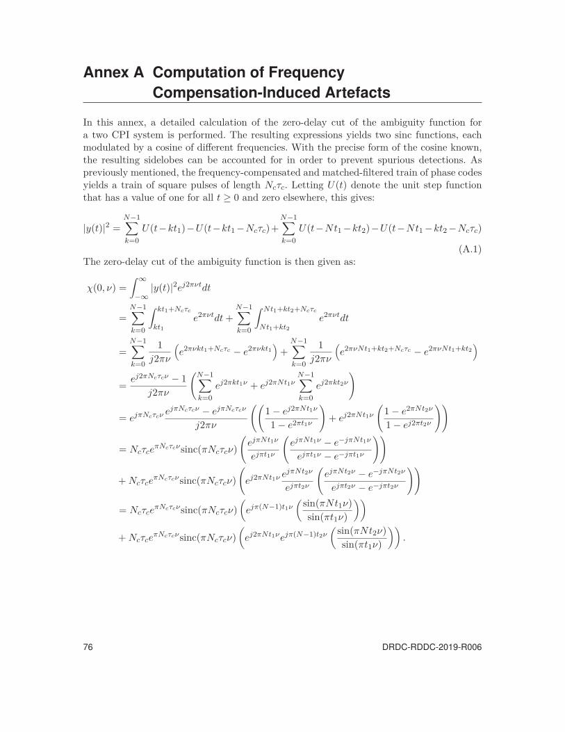
Annex A Computation of FrequencyCompensation-Induced Artefacts
In this annex, a detailed calculation of the zero-delay cut of the ambiguity function fora two CPI system is performed. The resulting expressions yields two sinc functions, eachmodulated by a cosine of different frequencies. With the precise form of the cosine known,the resulting sidelobes can be accounted for in order to prevent spurious detections. Aspreviously mentioned, the frequency-compensated and matched-filtered train of phase codesyields a train of square pulses of length Ncτc. Letting U(t) denote the unit step functionthat has a value of one for all t ≥ 0 and zero elsewhere, this gives:
|y(t)|2 =N−1∑k=0
U(t−kt1)−U(t−kt1 −Ncτc)+N−1∑k=0
U(t−Nt1 −kt2)−U(t−Nt1 −kt2 −Ncτc)
(A.1)The zero-delay cut of the ambiguity function is then given as:
χ(0, ν) =∫ ∞
−∞|y(t)|2ej2πνtdt
=N−1∑k=0
∫ kt1+Ncτc
kt1e2πνtdt +
N−1∑k=0
∫ Nt1+kt2+Ncτc
Nt1+kt2e2πνtdt
=N−1∑k=0
1j2πν
(e2πνkt1+Ncτc − e2πνkt1
)+
N−1∑k=0
1j2πν
(e2πνNt1+kt2+Ncτc − e2πνNt1+kt2
)
=ej2πNcτcν − 1
j2πν
(N−1∑k=0
ej2πkt1ν + ej2πNt1νN−1∑k=0
ej2πkt2ν
)
= ejπNcτcν ejπNcτcν − ejπNcτcν
j2πν
((1 − ej2πNt1ν
1 − e2πt1ν
)+ ej2πNt1ν
(1 − e2πNt2ν
1 − ej2πt2ν
))
= NcτceπNcτcνsinc(πNcτcν)
(ejπNt1ν
ejπt1ν
(ejπNt1ν − e−jπNt1ν
ejπt1ν − e−jπt1ν
))
+ NcτceπNcτcνsinc(πNcτcν)
(ej2πNt1ν ejπNt2ν
ejπt2ν
(ejπNt2ν − e−jπNt2ν
ejπt2ν − e−jπt2ν
))
= NcτceπNcτcνsinc(πNcτcν)
(ejπ(N−1)t1ν
(sin(πNt1ν)sin(πt1ν)
))
+ NcτceπNcτcνsinc(πNcτcν)
(ej2πNt1νejπ(N−1)t2ν
(sin(πNt2ν)sin(πt1ν)
)).
76 DRDC-RDDC-2019-R006

Finally,
Re{χ(0, ν)} = Ncτcsinc(πNcτcν)(
cos(π((N − 1)t1 + Ncτc)ν)(sin(πNt1ν)
sin(πt1ν)
))
+ Ncτcsinc(πNcτcν)(
cos(π(2Nt1 + (N − 1)t2 + Ncτc)ν)(sin(πNt2ν)
sin(πt2ν)
)).
(A.2)
Figures A.1 and A.2 shows the two summands of Eq. (A.2) evaluated for N = 129, Nc =20, τc = 6 · 10−8, t1 = 200τc, and t2 = 203τc for CPI 1 and 2 on identical axes respectively.Note that, although the first term in Eq. (A.2) has a modulating cosine, the frequency(f0 = ((N −1)t1+Ncτc)/2) is too low for it to have a noticeable effect on the mainlobe of thesinc function. On the other hand, the cosine of the second term has a high enough frequencyfor the mainlobe of the sinc term to be noticeably modulated. Terms for subsequent CPIwould show even greater degrees of modulation. Finally, for the sake of completeness, wenote that the sin(Nπtν)/ sin(πtν) terms cause periodic repetitions of the shape shown inFigure A.1 at intervals determined by the sinusoid in the denominator: see [96] (pp. 42–46)for details.
-2500 -2000 -1500 -1000 -500 0 500 1000 1500 2000 2500Frequency, Hz
-2
-1
0
1
2
Zero
-Del
ay C
ut A
mbi
guity
Fun
ctio
n R
espo
nse
10-4 Frequency Response, CPI 1
Figure A.1: A typical frequency-domain response for the first CPI, withN = 129, Nc = 20, τc = 6 · 10−8, and t1 = 200τc.
DRDC-RDDC-2019-R006 77

-2500 -2000 -1500 -1000 -500 0 500 1000 1500 2000 2500Frequency, Hz
-2
-1
0
1
2
Zero
-Del
ay C
ut A
mbi
guity
Fun
ctio
n H
eigh
t
10-4 Frequency Response, CPI 2
Figure A.2: A typical frequency-domain response for the second CPI, withN = 129, Nc = 20, τc = 6 · 10−8, and t2 = 203τc.
78 DRDC-RDDC-2019-R006

DOCUMENT CONTROL DATA*Security markings for the title, authors, abstract and keywords must be entered when the document is sensitive
1. ORIGINATOR (Name and address of the organization preparing thedocument. A DRDC Centre sponsoring a contractor’s report, or atasking agency, is entered in Section 8.)
DRDC – Ottawa Research Centre3701 Carling Avenue, Ottawa ON K1A 0Z4,Canada
2a. SECURITY MARKING (Overall security marking ofthe document, including supplemental markings ifapplicable.)
CAN UNCLASSIFIED
2b. CONTROLLED GOODS
NON-CONTROLLED GOODSDMC A
3. TITLE (The document title and sub-title as indicated on the title page.)
Dwell Time Minimization for Unambiguous Radar Range and Doppler Measurements
4. AUTHORS (Last name, followed by initials – ranks, titles, etc. not to be used. Use semi-colon as delimiter)
Daniel, A. M.
5. DATE OF PUBLICATION (Month and year of publication ofdocument.)
July 2019
6a. NO. OF PAGES (Totalpages, including Annexes,excluding DCD, coveringand verso pages.)
86
6b. NO. OF REFS (Totalcited in document.)
96
7. DOCUMENT CATEGORY (e.g., Scientific Report, Contract Report, Scientific Letter)
Scientific Report
8. SPONSORING CENTRE (The name and address of the department project or laboratory sponsoring the research anddevelopment.)
DRDC – Ottawa Research Centre3701 Carling Avenue, Ottawa ON K1A 0Z4, Canada
9a. PROJECT OR GRANT NO. (If appropriate, the applicableresearch and development project or grant number underwhich the document was written. Please specify whetherproject or grant.)
01bd
9b. CONTRACT NO. (If appropriate, the applicable contractnumber under which the document was written.)
10a. DRDC DOCUMENT NUMBER
DRDC-RDDC-2019-R00610b. OTHER DOCUMENT NO(s). (Any other numbers which may
be assigned this document either by the originator or by thesponsor.)
11a. FUTURE DISTRIBUTION WITHIN CANADA (Approval for further dissemination of the document. Security classification must alsobe considered.)
Public release
11b. FUTURE DISTRIBUTION OUTSIDE CANADA (Approval for further dissemination of the document. Security classification must alsobe considered.)
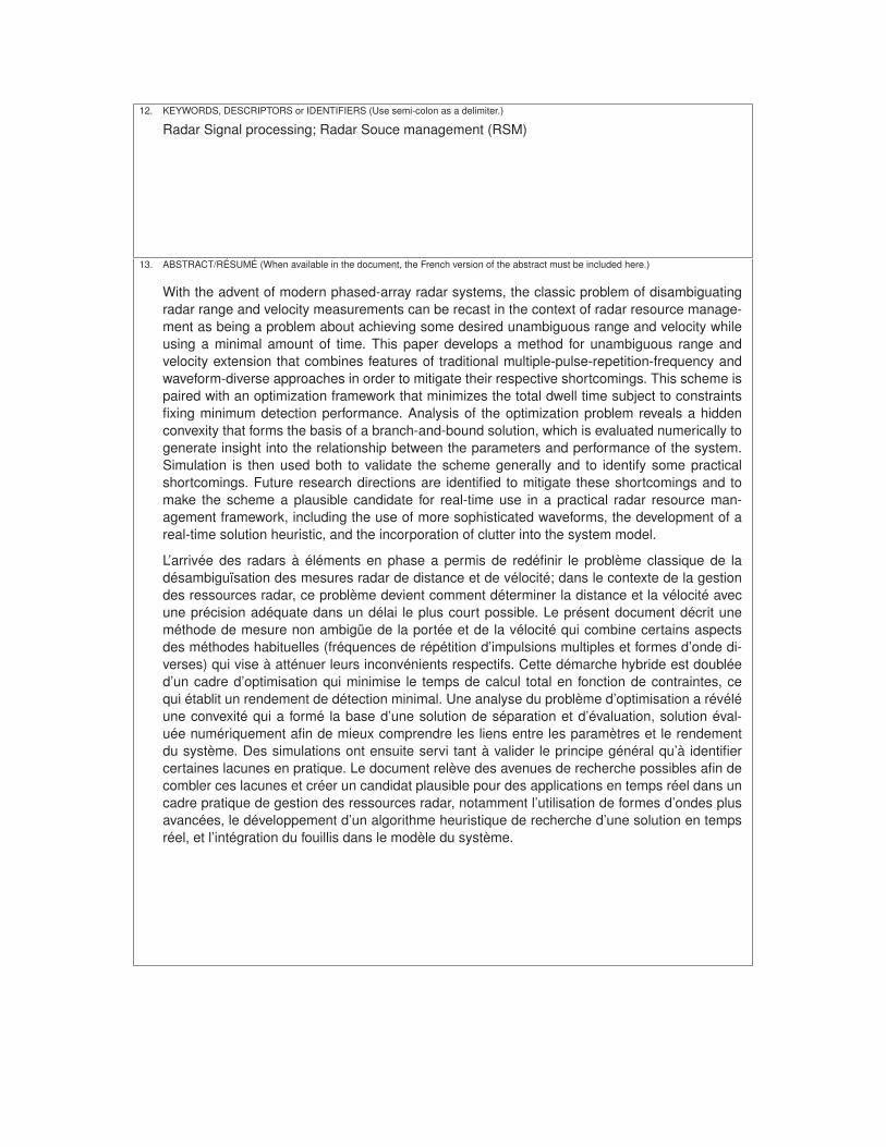
12. KEYWORDS, DESCRIPTORS or IDENTIFIERS (Use semi-colon as a delimiter.)
Radar Signal processing; Radar Souce management (RSM)
13. ABSTRACT/RÉSUMÉ (When available in the document, the French version of the abstract must be included here.)
With the advent of modern phased-array radar systems, the classic problem of disambiguatingradar range and velocity measurements can be recast in the context of radar resource manage-ment as being a problem about achieving some desired unambiguous range and velocity whileusing a minimal amount of time. This paper develops a method for unambiguous range andvelocity extension that combines features of traditional multiple-pulse-repetition-frequency andwaveform-diverse approaches in order to mitigate their respective shortcomings. This scheme ispaired with an optimization framework that minimizes the total dwell time subject to constraintsfixing minimum detection performance. Analysis of the optimization problem reveals a hiddenconvexity that forms the basis of a branch-and-bound solution, which is evaluated numerically togenerate insight into the relationship between the parameters and performance of the system.Simulation is then used both to validate the scheme generally and to identify some practicalshortcomings. Future research directions are identified to mitigate these shortcomings and tomake the scheme a plausible candidate for real-time use in a practical radar resource man-agement framework, including the use of more sophisticated waveforms, the development of areal-time solution heuristic, and the incorporation of clutter into the system model.
L’arrivée des radars à éléments en phase a permis de redéfinir le problème classique de ladésambiguïsation des mesures radar de distance et de vélocité; dans le contexte de la gestiondes ressources radar, ce problème devient comment déterminer la distance et la vélocité avecune précision adéquate dans un délai le plus court possible. Le présent document décrit uneméthode de mesure non ambigüe de la portée et de la vélocité qui combine certains aspectsdes méthodes habituelles (fréquences de répétition d’impulsions multiples et formes d’onde di-verses) qui vise à atténuer leurs inconvénients respectifs. Cette démarche hybride est doubléed’un cadre d’optimisation qui minimise le temps de calcul total en fonction de contraintes, cequi établit un rendement de détection minimal. Une analyse du problème d’optimisation a révéléune convexité qui a formé la base d’une solution de séparation et d’évaluation, solution éval-uée numériquement afin de mieux comprendre les liens entre les paramètres et le rendementdu système. Des simulations ont ensuite servi tant à valider le principe général qu’à identifiercertaines lacunes en pratique. Le document relève des avenues de recherche possibles afin decombler ces lacunes et créer un candidat plausible pour des applications en temps réel dans uncadre pratique de gestion des ressources radar, notamment l’utilisation de formes d’ondes plusavancées, le développement d’un algorithme heuristique de recherche d’une solution en tempsréel, et l’intégration du fouillis dans le modèle du système.