Embed Size (px)
Citation preview
DVRPC Travel Demand Model Upgrade - Travel Improvement Model (TIM) 1.0
January 2011

DVRPC Travel Demand Model Upgrade -Travel Improvement Model (TIM) 1.0
January 2011
190 N Independence Mall West ACP Building, 8th Floor Philadelphia, PA 19106-1520 Phone: 215-592-1800 Fax: 215-592-9125 Website: www.dvrpc.org
rait (3B) Template
The Delaware Valley Regional Planning Commission is dedicated to uniting the region’s elected officials, planning professionals, and the public with a common vision of making a great region even greater. Shaping the way we live, work, and play, DVRPC builds consensus on improving transportation, promoting smart growth, protecting the environment, and enhancing the economy. We serve a diverse region of nine counties: Bucks, Chester, Delaware, Montgomery, and Philadelphia in Pennsylvania; and Burlington, Camden, Gloucester, and Mercer in New Jersey. DVRPC is the federally designated Metropolitan Planning Organization for the Greater Philadelphia Region - leading the way to a better future.
The symbol in our logo is adapted from the official DVRPC seal and is designed as a stylized image of the Delaware Valley. The outer ring symbolizes the region as a whole while the diagonal bar signifies the Delaware River. The two adjoining crescents represent the Commonwealth of Pennsylvania and the State of New Jersey.
DVRPC is funded by a variety of funding sources including federal grants from the U.S. Department of Transportation’s Federal Highway Administration (FHWA) and Federal Transit Administration (FTA), the Pennsylvania and New Jersey Departments of Transportation, as well as by DVRPC’s state and local member governments. An original version of this report was authored by Thomas Rossi of Cambridge Systematics, Inc. (CSI) and Wolfgang Scherr of PTV America, Inc. (now with DVRPC) under contract with DVRPC. The report has been revised by DVRPC staff and CSI staff to reflect the current version of the model. The authors, however, are solely responsible for the findings and conclusions herein, which may not represent the official views or policies of the funding agencies.
DVRPC fully complies with Title VI of the Civil Rights Act of 1964 and related statutes and regulations in all programs and activities. DVRPC’s website (www.dvrpc.org) may be translated into multiple languages. Publications and other public documents can be made available in alternative languages and formats, if requested. For more information, please call (215) 238-2871.
D V R P C T r a v e l D e m a n d M o d e l U p g r a d e - T r a v e l I m p r o v e m e n t M o d e l ( T I M ) 1 . 0 i
Table of Contents
Executive Summary......................................................................................... 1
C H A P T E R 1 Introduction...................................................................................................... 3
C H A P T E R 2 Network and Zone Data................................................................................... 5 � 2.1 Zone Data ........................................................................................... 5 � 2.2 Network Translation from TRANPLAN to VISUM............................... 6 � 2.3 General Definitions of the VISUM Network....................................... 11 � 2.4 Highway and Transit Networks in Overview ..................................... 15 � 2.5 Integration of Complementary GIS Data........................................... 18
C H A P T E R 3 Trip Generation.............................................................................................. 19 � 3.1 Internal Non-Motorized Trips ............................................................ 20 � 3.2 Internal Person Trips......................................................................... 20 � 3.3 Internal Vehicle Trips ........................................................................ 20 � 3.4 External Trips.................................................................................... 20 � 3.5 Time of Day....................................................................................... 26 � 3.6 Implementation ................................................................................. 27
C H A P T E R 4 Trip Distribution ............................................................................................. 29 � 4.1. Impedance ....................................................................................... 29 � 4.2. Gravity Model................................................................................... 30 � 4.3. Adjustment to Trip Distribution for Transit Service
Quality ..................................................................................................... 32
C H A P T E R 5 Mode Choice ................................................................................................. 35 � 5.1 Supply Characteristics in Mode Choice ............................................ 36 � 5.2 Mode Captives and Auto Ownership ................................................ 37 � 5.3 Binary-Nested Mode Choice............................................................. 38 � 5.4 Vehicle Occupancy ........................................................................... 43
C H A P T E R 6 Assignment Models ....................................................................................... 45 � 6.1 Transit Assignment ........................................................................... 45 � 6.2 Transit Skimming .............................................................................. 47

D V R P C T r a v e l D e m a n d M o d e l U p g r a d e - T r a v e l I m p r o v e m e n t M o d e l ( T I M ) 1 . 0
i i
6.3 Highway Assignment ........................................................................ 47
6.4 Highway Skimming ........................................................................... 55
C H A P T E R 7
Combined Equilibrium ................................................................................... 57
7.1 Averaging of the Highway Impedance Matrix ................................... 57
7.2 Organization of the Feedback Loop.................................................. 58
7.3 Predefined Averaging Weights ......................................................... 58
7.4 Convergence Monitoring and Loop Termination .............................. 58
7.5 Different Averaging Methods ............................................................ 59
7.6 Final Feedback Parameters.............................................................. 63
C H A P T E R 8
Model Validation ............................................................................................ 67
8.1 Trip Distribution Validation................................................................ 67
8.2 Mode Choice Validation .................................................................... 70
8.3 Highway Assignment Validation ....................................................... 73
8.4 Transit Assignment Validation .......................................................... 74
C H A P T E R 9
Model Run Organization................................................................................ 79
9.1 Computer Requirements................................................................... 79
9.2 The Full Model Run with the Master Script....................................... 79
9.3 Model Procedure in Individual Steps ................................................ 82
9.4 Results, Reports, and Protocols of the Model Run........................... 86
9.5 Trip Purposes and Demand Stratification ......................................... 86
Figures and Tables Figure 1. Transit Network Import in VISUM.........................................................................9 Figure 2. VISUM Highway Network ...................................................................................15 Figure 3. VISUM Transit Network......................................................................................16 Figure 4. DVRPC Mode Choice Model as Flow Chart.......................................................35 Figure 5. Structure of the Nested Mode Choice ................................................................39 Figure 6. Transit Assignment Impedance Settings............................................................46 Figure 7. User Settings of the Path-Based Highway Assignment......................................50 Figure 8. Toll Plaza Volume-Delay Function .....................................................................53 Figure 9. Flow Chart of the Feedback Loop ......................................................................59 Figure 10. Relative Gap with Different Averaging Methods...............................................60 Figure 11. %RMSE-Demand with Different Averaging Methods .......................................61 Figure 12. %RMSE-Impedance with Different Averaging Methods ...................................61

D V R P C T r a v e l D e m a n d M o d e l U p g r a d e - T r a v e l I m p r o v e m e n t M o d e l ( T I M ) 1 . 0 i i i
Figure 13. Recommended Settings for Model Run Termination........................................64 Figure 14. Relative Gap with CW = 0.5 for All Three Time Periods...................................65 Figure 15. %RMSE-Demand with CW = 0.5 for All Three Time Periods ...........................65 Figure 16. %RMSE-Impedance with CW = 0.5 for All Three Time Periods.......................66 Figure 17. The Customized GUI for the DVRPC Model Run.............................................81 Table 1. Generalized Travel Modes in VISUM ..................................................................11 Table 2. Detailed Modes in VISUM (Transport Systems) ..................................................12 Table 3. Transit Operators in VISUM ................................................................................13 Table 4. Stop Types ..........................................................................................................13 Table 5. Link Types in VISUM...........................................................................................14 Table 6. Number of Lines, Line Routes, and Time Profiles in the Transit Network ...........17 Table 7. Area Types ..........................................................................................................19 Table 8. Internal Non-Motorized Trip Rates ......................................................................21 Table 9. Internal Motorized Person Trip Rates..................................................................22 Table 10. Non-Institutional Group Quarters Motorized Trip Rates ....................................23 Table 11. Trip Generation Rates for Truck and Taxi Trips ................................................24 Table 12. Temporal Factors to Disaggregate Daily Person Trip Generation Results ........26 Table 13. Temporal Factors to Disaggregate Vehicle Trip Generation Results.................26 Table 14. Trip Distribution Penalty Matrix..........................................................................30 Table 15. Gravity Model Parameters.................................................................................31 Table 16. Criteria and Percentage of Captive Travelers....................................................38 Table 17. Nested LOGIT Model Parameters for all Periods ..............................................40 Table 18. Nested LOGIT Model Constants for all Periods.................................................41 Table 19. Mode Choice Correction Variable "Impedance Factor" .....................................42 Table 20. Mode Choice Penalty Matrix..............................................................................42 Table 21. Coefficients of the Vehicle Occupancy Model ...................................................43 Table 22. Composition of the Total Highway Demand as Vehicle Trips ............................48 Table 23. Toll Plaza VDF Parameters in DVRPC's VISUM Model ....................................53 Table 24. Comparison of Different Averaging Methods.....................................................62 Table 25. Effective Feedback Parameters ........................................................................64 Table 26. Average Trip Length Comparison by Time Period.............................................68 Table 27. Average Daily Trip Length Comparison.............................................................69 Table 28. Transit Share Comparison by County ...............................................................70 Table 29. Mode Choice Comparison by Time Period........................................................71 Table 30. Vehicle Occupancy Rate Comparison...............................................................72 Table 31. VMT Comparison on All Links by County ..........................................................73 Table 32. Percentage Root Mean Square Estimates ........................................................74 Table 33. Screenline Summary .........................................................................................75 Table 34. Transit Assignment Validation Summary...........................................................76

D V R P C T r a v e l D e m a n d M o d e l U p g r a d e - T r a v e l I m p r o v e m e n t M o d e l ( T I M ) 1 . 0
i v
Table 35. Average Transit in Vehicle Trip Length Validation.............................................78 Table 36. Operations Procedure in Parameter File TripGen .............................................82 Table 37. Operations in Parameter File "Init" ....................................................................83 Table 38. Operations in Parameter File "Middle"...............................................................84 Table 39. Operations in Parameter File "End"...................................................................85 Table 40. Differences in the PAR Files Between Time Periods.........................................85 Table 41. Time of Day as "Persons Groups" in VISUM.....................................................87 Table 42. Trip Purposes as "Activity Pairs" in VISUM .......................................................88 Table 43. Demand Strata in VISUM for Trip Distribution and Mode Choice ......................89 Table 44. Demand Matrices and Skim Matrices................................................................89
Appendix Fare System Documentation.......................................................................A–1
Appendix Figures
Figure A-1.Adding Fare Points to Links to Mode Fare Zones.......................................... A-2 Figure A-2.Defining Tsys Supplements ........................................................................... A-3 Figure A-3.Connecting Put Tickets with Demand Segments........................................... A-4 Figure A-4.Instructing VISUM to Calulate Fare Separately for each Path Leg (transfer) A-5 Figure A-5.Defining Extra Boarding Charge by Tsys....................................................... A-6 Figure A-6.Setting up Extended Impedance so that Extra Charge for Boarding is Added .......................................................................................................................... A-7 Figure A-7.Defining Impedance Related Attributes on Drive to Transit Links.................. A-8

D V R P C T r a v e l D e m a n d M o d e l U p g r a d e - T r a v e l I m p r o v e m e n t M o d e l ( T I M ) 1 . 0 1
Executive Summary
The Delaware Valley Regional Planning Commission (DVRPC) is undertaking a multi-year project to upgrade the travel demand models that are used to forecast highway traffic and transit ridership in the region. The first result of this upgrade project is the migration of the model from the TRANPLAN software to the VISUM software package. This work has been undertaken by Cambridge Systematics, Inc. (CS) and PTV America, Inc. under contract to DVRPC. DVRPC staff contributed the future year networks and the socio-demographic forecasts.
This report documents the resulting model in VISUM. This model is called the Travel Improvement Model Version 1.0 (TIM 1.0). TIM 1.0 is based on DVRPC’s current system of 2068 traffic analysis zones. Many model components of TIM 1.0 remain unchanged from the legacy TRANPLAN model, in particular trip generation and trip distribution. Other model components, including mode choice, highway assignment and transit assignment went through significant changes and upgrades, which was necessary to accommodate the model under the new software platform. Major benefits from the migration to VISUM include better graphics and mapping, automated QA/QC and convergence of the highway travel times which is beneficial in the comparison of network scenarios.
TIM 1.0 has been used for all new transportation projects that started after April 2010. TIM 1.0 will continue to be used through all of 2011 until the next model upgrade which is expected in the second half of 2011.

D V R P C T r a v e l D e m a n d M o d e l U p g r a d e - T r a v e l I m p r o v e m e n t M o d e l ( T I M ) 1 . 0 3
C H A P T E R 1
Introduction
The Delaware Valley Regional Planning Commission (DVRPC) is undertaking a project to upgrade the Commission’s travel demand models. The first step in this process is the conversion of the modeling software from TRANPLAN to the VISUM software package. This work has been undertaken by Cambridge Systematics, Inc. (CS) and PTV America, Inc. under contract to DVRPC.
Travel modeling is performed by DVRPC for a number of different purposes. The main purposes are the development of long- and short-range plans and programs, highway traffic studies, air quality conformity demonstrations, Federal Transit Administration (FTA) New Starts programs, and member government transportation studies. The travel forecasting models are guided by Federal Highway Administration (FHWA), Environmental Protection Agency (EPA), and Federal Transit Administration (FTA) guidelines. The travel forecasting models are mostly run by DVRPC staff. The models are also used by outside consultants with DVRPC assistance.
This report documents the converted VISUM model called the Travel Improvement Model (TIM), version 1.0. The report is organized by model function. Chapter 2 describes the network and zonal data used in the model. Chapters 3 through 6 document the four steps in the modeling process: trip generation, trip distribution, mode choice, and trip assignment, respectively. Chapter 7 discusses the combined equilibrium (feedback) approach for iteration of the model. Chapter 8 discusses the validation of the converted model, while Chapter 9 presents the mechanics of running the model.
Since most of the modeling processes in TIM 1.0 remain unchanged from those used in TRANPLAN, the report does not duplicate the complete documentation previously prepared by DVRPC1. Rather, the focus is on the differences in the modeling procedures that were made when the model was implemented in VISUM. Changes were made either when the two software package’s differing features required a change, or when VISUM had functionality that enabled a significant improvement in model performance at little cost.
The numbers in this report, such as parameters and validation results, reflect the 4/13/2010 release version of the model. The next major release of the model is expected in Summer 2011.
1 Delaware Valley Regional Planning Commission. 2000 and 2005 Validation of
the DVRPC Regional Simulation Models. July 2008.

D V R P C T r a v e l D e m a n d M o d e l U p g r a d e - T r a v e l I m p r o v e m e n t M o d e l ( T I M ) 1 . 0 5
C H A P T E R 2
Network and Zone Data
2.1 Zone Data
The zonal level data used in the VISUM implementation of the DVRPC model is the same as the data used in the TRANPLAN implementation. The zone data are stored in the “zones” object in VISUM. The following user-defined attributes (UDAs) were defined for the zone object in the DVRPC VISUM model:
� DISTRICT – County Planning Area (75 = external) � POPULATION – Total population � GROUPQUARTERS – Group quarters population � HOUSEHOLDS – Number of households � VEHICLES – Total number of vehicles in all households � AGRICULTURE, MINING, CONSTRUCTION, MANUFACTURING,
TRANSPORTATION, WHOLESALE, RETAIL, FIRE, SERVICE, GOVERNMENT, MILITARY – Total employment for each type working in zone
� AREA_TYPE – Per DVRPC definition (see Section III.D of the DVRPC documentation report)
� AUTO_0_HH – Number of households with zero autos � AUTO_1_HH – Number of households with one auto � AUTO_2_HH – Number of households with two autos � AUTO_3P_HH – Number of households with three or more autos � EMPLOYED_PERSONS – Number of employed persons living in zone � TOTAL_EMP – Total employment working in zone � VOL1 – External station volume (through traffic) � VOL2 – External station volume (external-internal traffic) � E_TYPE – External station type (1 = freeway, 2 = arterial, 3 = local, 4 =
turnpike) � TPK_STA – Nearest turnpike external station number to zone � TPK_DIST – Distance from centroid to TPK_STA � FWY_STA – Nearest freeway external station number to zone � FWY_DIST – Distance from centroid to FWY_STA � ART_STA – Nearest arterial external station number to zone � ART_DIST – Distance from centroid to ART_STA � LOC_STA – Nearest local external station number to zone � LOC_DIST – Distance from centroid to LOC_STA � HH0CAR_HBW – Share of 0-car households for trip purpose HBW
6 D V R P C T r a v e l D e m a n d M o d e l U p g r a d e - T r a v e l I m p r o v e m e n t M o d e l ( T I M ) 1 . 0
� HH0CAR_HBNW – Share of 0-car households for trip purpose HBNW � HH0CAR_NHB – Share of 0-car households for trip purpose NHB � STATE – (42 = Pennsylvania, 34 = New Jersey) � COUNTY – County code � EXT_PEAK – Percentage of volume occurring in peak period for external
zone � EXT_MD – Percentage of volume occurring in mid-day period for
external zone � EXT_NT – Percentage of volume occurring in evening period for external
zone � PARKINGCOST – Parking cost per day in dollars � LATF – Local external attraction factor applied to traffic zones less than 6
miles from the cordon station (see Appendix VII-5 of the DVRPC documentation report and Section 3.2 of this report)
2.2 Network Translation from TRANPLAN to VISUM
The complexity of the DVRPC model went to the edge of TRANPLAN’s software capabilities and sometimes beyond, so that DVRPC’s modelers had to add customized tools to complement the TRANPLAN package.
The most important benefit from the software platform change is VISUM’s network data management: VISUM integrates all network objects and layers for highway and transit over all time periods into one single file. All objects are interconnected within the Version (VER) file using VISUM’s internal database. As a result, edits to one object, for example on links or nodes, are instantly translated into updates of related linked objects, for example transit time profiles.
In TRANPLAN, highway and transit are not integrated and there is no ability to store data for several times of day in parallel. As a result, nine separate TRANPLAN network files had to be matched and integrated into one single VISUM data model: three highway network files (peak, midday, evening), three “normal” transit networks, and three “shadow” transit networks.
The process of building a VISUM network that integrates the TRANPLAN highway network with multiple transit networks is highly complex. While the highway translation is straightforward and was largely automated, the transit integration involved many steps. The step-by-step translation processes for the highway and transit networks are described below.
Translation of Highway Networks Step-by-Step
1. Translate highway nodes and links provided as TRANPLAN text files using VISUM’s CUBE importer, which creates a VISUM network with nodes, zones, links, and connectors.

D V R P C T r a v e l D e m a n d M o d e l U p g r a d e - T r a v e l I m p r o v e m e n t M o d e l ( T I M ) 1 . 0 7
2. Determine link and connector attributes using an Excel spreadsheet, which for 2005 was prepared by PTV America during the translation of the 2005 case and can be applied to any other DVRPC network.
a. Set the most important VISUM link attributes: TypeNo, CAP_24H, v0 (free flow speed), Length, Toll, NumLanes
b. In addition, set some secondary, informative attributes such as DVRPC_FClass, Fed_FClass, and DVRPC_AreaType
c. For toll plaza links, translate a separate TRANPLAN data file to determine the VISUM attributes: TypeNo, CAP_24H, v0
d. Translate attributes for VISUM connectors, which are a subset of the TRANPLAN links, mainly length and t0 (free flow time)
e. From the Excel spreadsheet, copy the attribute listings into VISUM over the Windows Clipboard
f. Use VISUM GIS to calculate true link length and replace link length imported from TRANPLAN for all links except ramps
3. Test the translated network by running a highway assignment in VISUM as follows:
a. Import highway trip matrices, which correspond to the translated network, from TRANPLAN text files, using a VBS script provided by PTV
b. Read assignment parameters with a PAR file
c. Determine the capacity that is used for assignment as a percentage of CAP_24H
d. Run assignments with fixed trip table for all three time periods (PK, MD, EV)
e. Compare the resulting link volumes with the TRANPLAN volumes
f. Identify and correct eventual translation errors
Translation of Transit Networks Step-by-Step
1. Create a VISUM network with all highway nodes plus all complementary transit nodes (rail stations and rail shape nodes). For the 2005 case, there were 18,177 highway nodes and 1,938 complementary transit nodes.
2. Develop connectors and access links:
a. Open connectors for one or both of the PuTWalk transport systems (Walk-Access for transit-walk or “limited Auto-Access” for transit-auto).
8 D V R P C T r a v e l D e m a n d M o d e l U p g r a d e - T r a v e l I m p r o v e m e n t M o d e l ( T I M ) 1 . 0
b. Open access links mainly for PuTWalk, except for the case of the long auto access links, which are opened for the PuTAux system “Auto Approach”.
3. For six TRANPLAN transit networks (for the three time periods times two subnetworks, normal and shadow), the following steps need to be performed:
a. Using VISUM’s CUBE importer, import the CUBE/VIPER transit route file into this network which consists only of nodes. The importer will create all necessary links and set the VISUM link type to 99. The necessary VISUM settings are shown in Figure 1.
b. As a result, there will be transit routes in VISUM, including stop sequence, headway, TRANPLAN mode ID, TRANPLAN route name, and route number. Carefully read all error messages and take care of routes that were not imported because of missing nodes.
c. Delete stops that have been created by the importer but are not used by any line.
d. Import TRANPLAN hudnet.lnk file as VISUM TimeProfileItems with segment run times and segment distances for 15 TRANPLAN modes. This can be done with the help of a spreadsheet.
e. Create temporary UDA’s.
� From = LineRouteItem/NodeNo
� To = LineRouteItem/Next Route Point/NodeNo
� Tranpl_RunTime
� Tranpl_Length
f. Merge transit routes and TimeProfile run times in Excel to obtain complete LineRoutes and TimeProfiles in VISUM. In VISUM, update TimeProfileItem run-time from import variable Tranpl_RunTime.
g. Make sure that in the Peak network, all VISUM TimeProfiles have the name “AM” (and “Mid” and “Eve” in the other two time period networks).
4. As a result, there will be six VISUM VER files for the six transit network cases, which are kept separate at this time. These transit networks should be error-checked and tested as follows:
a. Compare total route run-time and total route length between TRANPLAN and VISUM. Differences result mainly on individual route segments that were not matched correctly. In case of major differences, parts of the import steps need to be revised and repeated or the data can be corrected with manual editing in VISUM.

D V R P C T r a v e l D e m a n d M o d e l U p g r a d e - T r a v e l I m p r o v e m e n t M o d e l ( T I M ) 1 . 0 9
Figure 1. Transit Network Import in VISUM
VISUM settings to read LineRoutes additionally into the highway network: links of type 99 are created in case no path through the network is found.
Finally, routes are created with time profiles for each time of day where the route has been used. In this example, the route has three time profiles: AM, MD, and EV.
Source: DVRPC January 2011
1 0 D V R P C T r a v e l D e m a n d M o d e l U p g r a d e - T r a v e l I m p r o v e m e n t M o d e l ( T I M ) 1 . 0
b. Perform a transit assignment in VISUM to check for errors in network connectivity:
� Import transit trip matrices from TRANPLAN text files, both for auto-access and walk-access, using a VISUAL BASIC script provided by PTV America
� Run the assignment
� Detect and correct network translation errors by focusing on nonassigned trips or differences between the TRANPLAN and VISUM assignment results
Integration of Highway and Transit Networks for All Three Time Periods
The imported highway and transit networks for all three time periods are integrated into one VISUM network model following these steps:
1. For each of the time periods, integrate highway and transit as follows:
a. Start with highway network as the basis
b. Add transit TSys and operators
c. Read complementary transit nodes as NET file
d. Read all stops, stop-areas, and stop-points as NET file
e. Auto and walk access links, connectors
f. Read Lines, LineRoutes, TimeProfiles, LineRouteItems, and TimeProfileItems as NET file. Choose VISUM option that links are created on the fly in case that no path for the line is found
g. Create and import user-defined attributes for the LineRoutes with the TRANPLAN information such as mode, ID, headway
h. Rename and group TRANPLAN routes to VISUM Lines:
� Develop matching table for TRANPLAN route ID to comprehensive line and route names in VISUM. Then rename
� Assign TRANPLAN mode to VISUM TSys
2. Merge all line routes from all three time periods into one network so that routes can have different time profiles for different times of day.
3. For error checking, mainly a comparison of total run-time per route was performed between TRANPLAN and VISUM.

D V R P C T r a v e l D e m a n d M o d e l U p g r a d e - T r a v e l I m p r o v e m e n t M o d e l ( T I M ) 1 . 0 1 1
Refinement of the TRANPLAN Network Data After Import
The following items were not performed for the 2005 network translation but may be done to enhance networks in the future:
1. Links can be shaped to represent the true topological form of streets. At the time of this report, this has been performed to a limited extent.
2. TRANPLAN shape nodes (two-arm nodes, which do not represent an intersection) can be deleted in VISUM by an automated procedure which converts them into link shape points.
3. Almost all VISUM objects, like zones, stops, and links can have names. It is recommended to add names to the network, which will increase the comprehensiveness of the model.
2.3 General Definitions of the VISUM Network
In the design of a VISUM network model, two important definitions are Modes and Transport Systems (TSys). The “mode” in VISUM mainly defines classes in the assignment models. For DVRPC, three modes have been defined, as shown in Table 1.
Table 1. Generalized Travel Modes in VISUM
Code Name
TW Transit Walk
TA Transit Auto
TX Transit External
Hwy Highway Car
Source: DVRPC January 2011 VISUM uses TSys to define differences in network conditions among different means of transportation. These differences include highway speeds, highway restrictions, transit run-times, transit restrictions on links, turns, nodes, and stops. Also, in the current VISUM version, TSys are used to define fare system classes, as shown in Table 2.
1 2 D V R P C T r a v e l D e m a n d M o d e l U p g r a d e - T r a v e l I m p r o v e m e n t M o d e l ( T I M ) 1 . 0
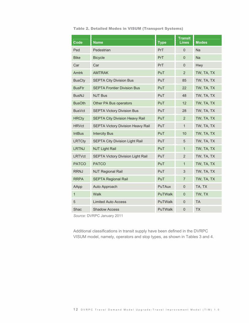
Table 2. Detailed Modes in VISUM (Transport Systems)
Source: DVRPC January 2011
Additional classifications in transit supply have been defined in the DVRPC VISUM model, namely, operators and stop types, as shown in Tables 3 and 4.
Code Name Type Transit Lines Modes
Ped Pedestrian PrT 0 Na
Bike Bicycle PrT 0 Na
Car Car PrT 0 Hwy
Amtrk AMTRAK PuT 2 TW, TA, TX
BusCty SEPTA City Division Bus PuT 85 TW, TA, TX
BusFtr SEPTA Frontier Division Bus PuT 22 TW, TA, TX
BusNJ NJT Bus PuT 48 TW, TA, TX
BusOth Other PA Bus operators PuT 12 TW, TA, TX
BusVct SEPTA Victory Division Bus PuT 28 TW, TA, TX
HRCty SEPTA City Division Heavy Rail PuT 2 TW, TA, TX
HRVct SEPTA Victory Division Heavy Rail PuT 1 TW, TA, TX
IntBus Intercity Bus PuT 10 TW, TA, TX
LRTCty SEPTA City Division Light Rail PuT 5 TW, TA, TX
LRTNJ NJT Light Rail PuT 1 TW, TA, TX
LRTVct SEPTA Victory Division Light Rail PuT 2 TW, TA, TX
PATCO PATCO PuT 1 TW, TA, TX
RRNJ NJT Regional Rail PuT 3 TW, TA, TX
RRPA SEPTA Regional Rail PuT 7 TW, TA, TX
AApp Auto Approach PuTAux 0 TA, TX
1 Walk PuTWalk 0 TW, TX
5 Limited Auto Access PuTWalk 0 TA
Shac Shadow Access PuTWalk 0 TX
D V R P C T r a v e l D e m a n d M o d e l U p g r a d e - T r a v e l I m p r o v e m e n t M o d e l ( T I M ) 1 . 0 1 3
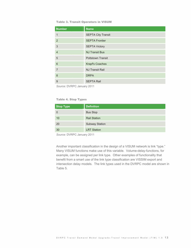
Table 3. Transit Operators in VISUM
Number Name
1 SEPTA City Transit
2 SEPTA Frontier
3 SEPTA Victory
4 NJ Transit Bus
5 Pottstown Transit
6 Krapf's Coaches
7 NJ Transit Rail
8 DRPA
9 SEPTA Rail
Source: DVRPC January 2011
Table 4. Stop Types
Stop Type Definition
0 Bus Stop
10 Rail Station
20 Subway Station
30 LRT Station
Source: DVRPC January 2011
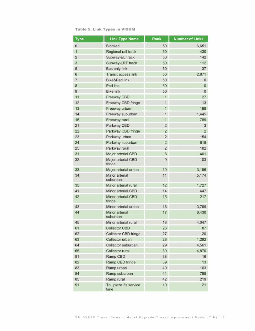
Another important classification in the design of a VISUM network is link “type.” Many VISUM functions make use of this variable. Volume-delay-functions, for example, can be assigned per link type. Other examples of functionality that benefit from a smart use of the link type classification are VISSIM export and intersection delay models. The link types used in the DVRPC model are shown in Table 5.
1 4 D V R P C T r a v e l D e m a n d M o d e l U p g r a d e - T r a v e l I m p r o v e m e n t M o d e l ( T I M ) 1 . 0
Table 5. Link Types in VISUM
Type Link Type Name Rank Number of Links
0 Blocked 50 6,6511 Regional rail track 50 4302 Subway-EL track 50 1423 Subway-LRT track 50 1125 Bus only link 50 376 Transit access link 50 2,8717 Bike&Ped link 50 08 Ped link 50 09 Bike link 50 011 Freeway CBD 1 2712 Freeway CBD fringe 1 1313 Freeway urban 1 19814 Freeway suburban 1 1,44515 Freeway rural 1 78921 Parkway CBD 2 322 Parkway CBD fringe 2 223 Parkway urban 2 15424 Parkway suburban 2 81825 Parkway rural 2 18231 Major arterial CBD 8 40132 Major arterial CBD
fringe 9 103
33 Major arterial urban 10 3,15634 Major arterial
suburban 11 5,174
35 Major arterial rural 12 1,72741 Minor arterial CBD 14 44742 Minor arterial CBD
fringe 15 217
43 Minor arterial urban 16 3,76944 Minor arterial
suburban 17 6,430
45 Minor arterial rural 18 4,04761 Collector CBD 26 8762 Collector CBD fringe 27 2063 Collector urban 28 1,29264 Collector suburban 29 4,56165 Collector rural 30 4,87081 Ramp CBD 38 1682 Ramp CBD fringe 39 1383 Ramp urban 40 16384 Ramp suburban 41 78585 Ramp rural 42 21991 Toll plaza 3s service
time 10 21
D V R P C T r a v e l D e m a n d M o d e l U p g r a d e - T r a v e l I m p r o v e m e n t M o d e l ( T I M ) 1 . 0 1 5
Source: DVRPC January 2011
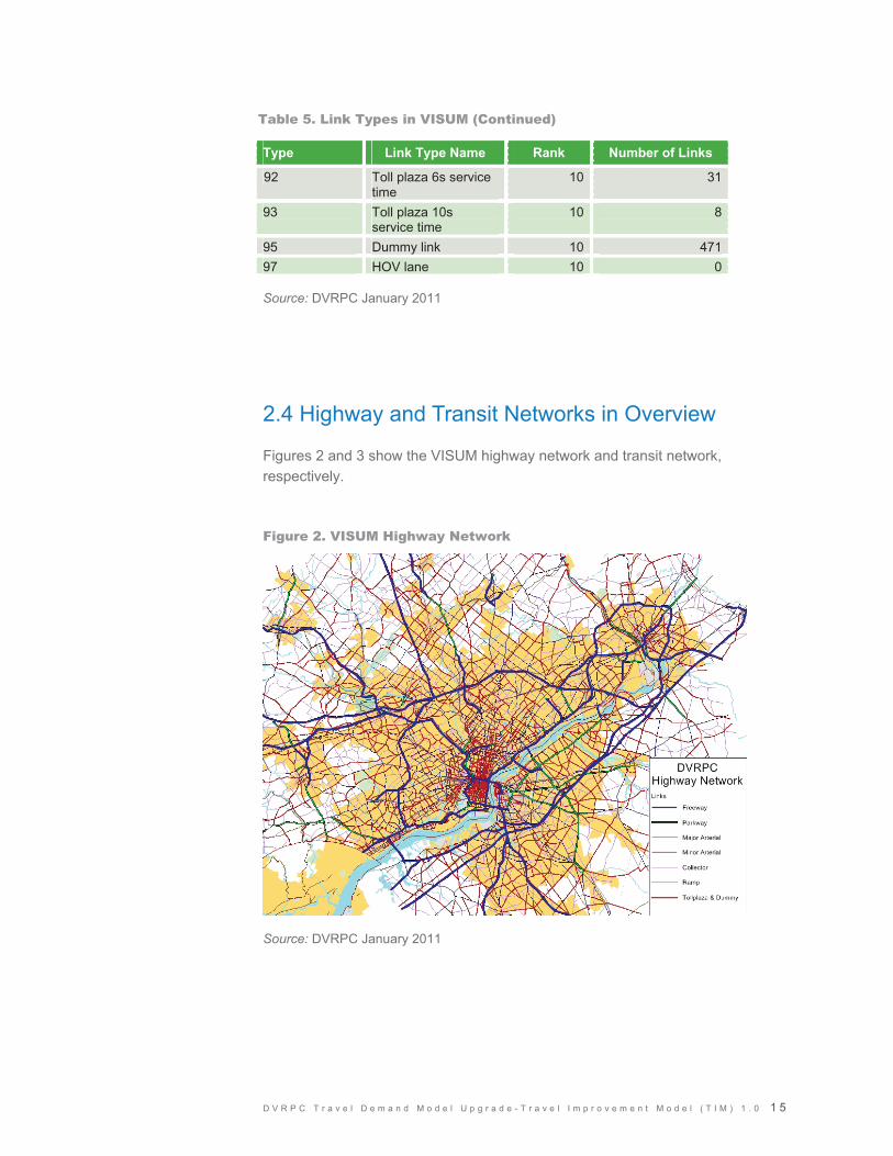
2.4 Highway and Transit Networks in Overview
Figures 2 and 3 show the VISUM highway network and transit network, respectively.
Figure 2. VISUM Highway Network
Source: DVRPC January 2011
Type Link Type Name Rank Number of Links
92 Toll plaza 6s service time
10 31
93 Toll plaza 10s service time
10 8
95 Dummy link 10 47197 HOV lane 10 0
Table 5. Link Types in VISUM (Continued)

1 6 D V R P C T r a v e l D e m a n d M o d e l U p g r a d e - T r a v e l I m p r o v e m e n t M o d e l ( T I M ) 1 . 0
Figure 3. VISUM Transit Network
Source: DVRPC January 2011
The VISUM transit network has 229 lines, 978 line routes, and 1,675 time profiles. The original TRANPLAN data has only one level of data, called “routes,” which corresponds to the VISUM line route. If several TRANPLAN routes belong to the same service, they were grouped under the same line in VISUM. If a route occurred in TRANPLAN for several times of day, time profiles were created that differentiate the route in terms of run-times and service headway.
Table 6 summarizes the number of lines, line routes, and time profiles in the VISUM transit network. Details on the coding of transit fares in TIM 1.0 are presented in the Appendix.

Tsys
Ts
ys N
ame
Num
ber o
f Li
nes
Line
Net
wor
k Le
ngth
, U
ndire
cted
(Mile
s)
Num
ber o
f R
oute
s N
umbe
r of
Tim
e Pr
ofile
s
Am
trk
AM
TRA
K
214
4.3
1720
RR
NJ
NJT
Reg
iona
l Rai
l 3
49.3
1020
RR
PA
S
EP
TA R
egio
nal R
ail
728
6.5
7088
HR
Cty
S
EP
TA C
ity D
ivis
ion
Hea
vy R
ail
223
.814
26
HR
Vct
S
EP
TA V
icto
ry D
ivis
ion
Hea
vy R
ail
112
.810
14
PA
TCO
P
ATC
O
113
.47
9
LRTC
ty
SE
PTA
City
Div
isio
n Li
ght R
ail
530
.425
37
LRTN
J N
JT L
ight
Rai
l 1
32.7
26
LRTV
ct
SE
PTA
Vic
tory
Div
isio
n Li
ght R
ail
213
.58
16
IntB
us
Inte
rcity
Bus
10
1147
.740
72
Bus
Cty
S
EP
TA C
ity D
ivis
ion
Bus
85
969.
337
067
2
Bus
Ftr
SE
PTA
Fro
ntie
r Div
isio
n B
us
2240
4.8
8314
4
Bus
Vct
S
EP
TA V
icto
ry D
ivis
ion
Bus
28
395.
010
318
1
Bus
NJ
NJT
Bus
48
1293
.118
431
3
Bus
Oth
P
A B
us O
pera
tors
12
107.
835
57
�Sou
rce:
DV
RP
C �
����
���
��
Tab
le 6
. Num
ber
of L
ines
, Lin
e R
oute
s, a
nd T
ime
Pro
file
s in
the
Tra
nsit
Net
wor
k
�
� � � � � � � � � � � � � � � � � � � � � � � � � � � � � � � � � � � � � � � � � � � � � � � � � � � � � � � � � � � � � � � � ! � � " �
�
�������������������������������� �

1 8 D V R P C T r a v e l D e m a n d M o d e l U p g r a d e - T r a v e l I m p r o v e m e n t M o d e l ( T I M ) 1 . 0
2.5 Integration of Complementary GIS Data
The translation of DVRPC’s network models to VISUM allows for geographically accurate representation and also for attractive mapping, which is equivalent to commercial GIS software. Also, VISUM allows the user to complement the network with GIS layers which do not necessarily influence the model results but help to make the network more comprehensive.
All data in the VISUM files have been translated into one coordinate system, which has been identified by DVRPC as the most suitable to store planning data for the DVRPC region:
� UTM 18N, Unit = Meter, NAD 1983
� Network length units are the typical U.S. units: Miles and miles per hour
� The VISUM “scale factor” is set to 0.621371, which converts the coordinate unit meter to length unit mile
Several complementary GIS layers have been added to the VISUM network:
� Traffic Analysis Zones (TAZ) boundaries (VISUM zone layer)
� District boundaries for “County Planning Areas” (VISUM territories and main zones)
� District boundaries for Counties and Municipalities (VISUM territories)
� NAVTEQ background layers (VISUM POI) for multiple layers such as rivers, creeks, lakes, canals, parks, cemeteries, golf clubs, airports, hospitals, shopping centers, sport courts, industrial areas, and urbanized areas
To enable quick and comprehensive mapping with the new DVRPC model, several VISUM graphic parameter files (GPA) have been developed to display the DVRPC network, assignment results, geography, land use data, etc. These GPA files are part of the model data set.
D V R P C T r a v e l D e m a n d M o d e l U p g r a d e - T r a v e l I m p r o v e m e n t M o d e l ( T I M ) 1 . 0 1 9
C H A P T E R 3
Trip Generation
In the DVRPC model, trip generation has two parts: motorized and non-motorized trips. The non-motorized trips are not differentiated by time of day. They are stored as zonal results and do not get translated into Origin destination matrices. Only the motorized trips continue through trip distribution and mode choice. Motorized trips are generated as either person trips or vehicle trips, depending on trip purpose. The person trip purposes are home-based work (HBW), home-based non-work (HBNW), non-home-based (NHB), and external transit trips. The vehicle trip types are light truck, heavy truck, and taxi trips, as well as the four external-internal vehicle trip types. These are turnpike external-internal vehicle trips, freeway/expressway external-internal vehicle trips, arterial external-internal vehicle trips, and local street external-internal vehicle trips.
Trip ends are estimated for each trip purpose. These trip ends take two forms depending on the trip purpose—productions and attractions or origins and destinations. Home-based trips are generated in production-attraction format where the home always produces the trip (even the trip to home), and the non-home end attracts the trip. Other types of trips are produced in origin-destination format. For external-internal trips all productions occur on the nine-county cordon line at external zones, and all corresponding attractions are allocated to internal traffic zones. Trip rates are typically differentiated according to six area types, which are shown in Table 7.
Table 7. Area Types
Area Type Explanation
1 Central Business District (CBD)
2 CBD fringe
3 Urban
4 Suburban
5 Rural
6 Open rural
Source: DVRPC January 2011
2 0 D V R P C T r a v e l D e m a n d M o d e l U p g r a d e - T r a v e l I m p r o v e m e n t M o d e l ( T I M ) 1 . 0
Chapter VII of the DVRPC report on the 2000 and 2005 VALIDATION of the DVRPC REGIONAL SIMULATION MODELS provides more information on the trip generation model, including how the trip rates were estimated, how the area types are defined as a function of density, and the use of special generators.
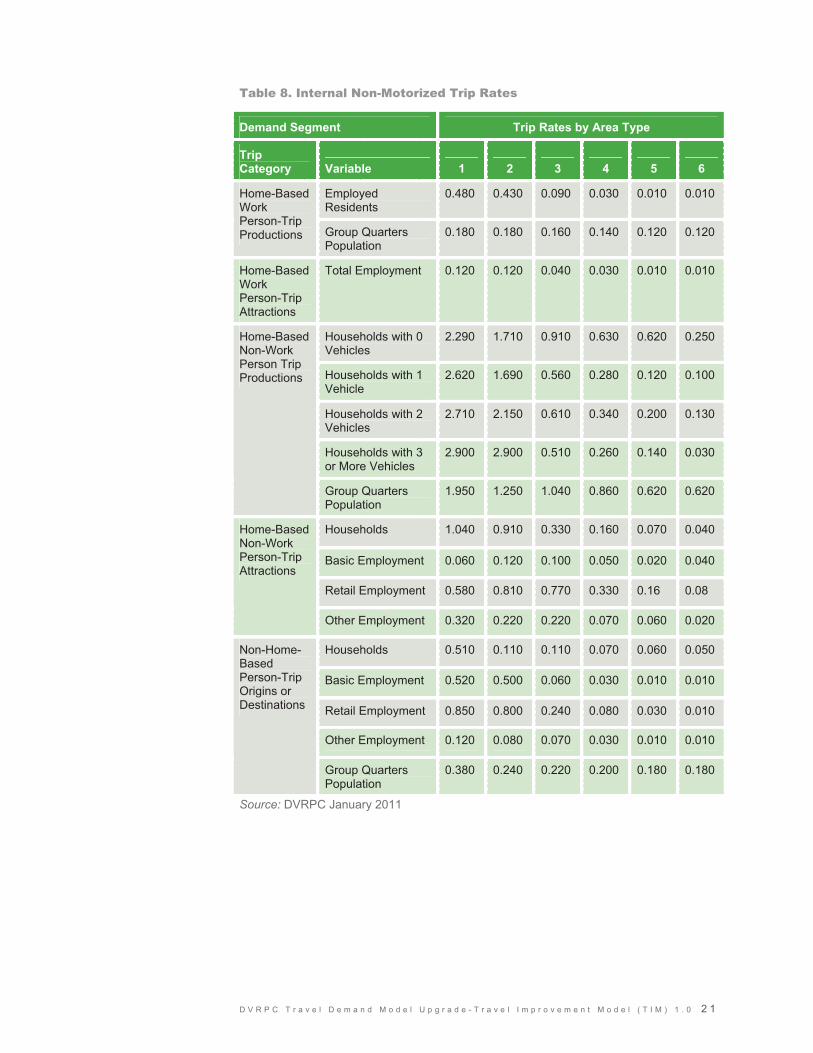
3.1 Internal Non-Motorized Trips
Table 8 presents the person trip generation rates for non-motorized trips of the three-person trip purposes.
3.2 Internal Person Trips
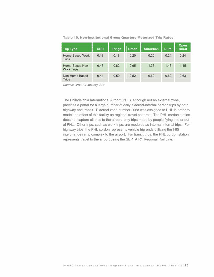
Table 9, which reproduces Table VII-2 from the DVRPC report, presents the person trip generation rates for internal motorized trips of the three-person trip purposes. Internal person trips are also generated for group quarters population; these rates are shown in Table 10 (reproduced from Table VII-3 in the DVRPC report).
Notes: For home-based, non-work attractions, total employment excludes military employment; for home-based non-work attractions, basic employment includes agricultural, mining, construction, manufacturing, and wholesale employment; for non-home-based trips, basic employment includes the same employment categories as for home-based, non-work attractions, except for mining, which is included in other employment.
3.3 Internal Vehicle Trips
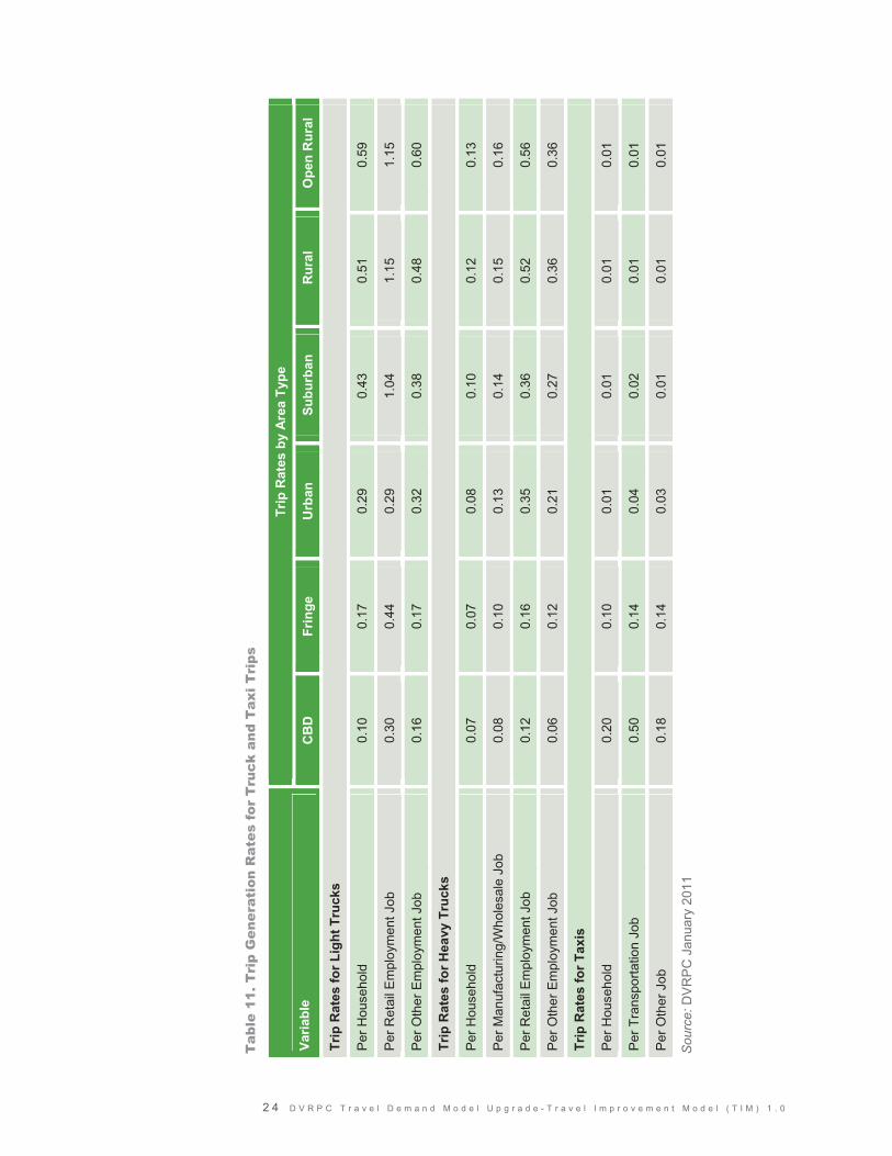
Table 11 shows the trip generation rates for truck and taxi trips (reproduced from Table VII-7 in the DVRPC report).
3.4 External Trips
External-internal highway trips are produced at the external zone and attracted to the internal zone. The internal trip ends are estimated based on trip rates tied to socio-economic variables. External trip ends at the cordon stations are determined directly by counts and surveys. External-internal highway trips are modeled as vehicle trips.
D V R P C T r a v e l D e m a n d M o d e l U p g r a d e - T r a v e l I m p r o v e m e n t M o d e l ( T I M ) 1 . 0 2 1
Table 8. Internal Non-Motorized Trip Rates
Demand Segment Trip Rates by Area Type
Trip Category Variable 1 2 3 4 5 6
Employed Residents
0.480 0.430 0.090 0.030 0.010 0.010 Home-Based Work Person-Trip Productions Group Quarters
Population 0.180 0.180 0.160 0.140 0.120 0.120
Home-Based Work Person-Trip Attractions
Total Employment 0.120 0.120 0.040 0.030 0.010 0.010
Households with 0 Vehicles
2.290 1.710 0.910 0.630 0.620 0.250
Households with 1 Vehicle
2.620 1.690 0.560 0.280 0.120 0.100
Households with 2 Vehicles
2.710 2.150 0.610 0.340 0.200 0.130
Households with 3 or More Vehicles
2.900 2.900 0.510 0.260 0.140 0.030
Home-Based Non-Work Person Trip Productions
Group Quarters Population
1.950 1.250 1.040 0.860 0.620 0.620
Households 1.040 0.910 0.330 0.160 0.070 0.040
Basic Employment 0.060 0.120 0.100 0.050 0.020 0.040
Retail Employment 0.580 0.810 0.770 0.330 0.16 0.08
Home-Based Non-Work Person-Trip Attractions
Other Employment 0.320 0.220 0.220 0.070 0.060 0.020
Households 0.510 0.110 0.110 0.070 0.060 0.050
Basic Employment 0.520 0.500 0.060 0.030 0.010 0.010
Retail Employment 0.850 0.800 0.240 0.080 0.030 0.010
Other Employment 0.120 0.080 0.070 0.030 0.010 0.010
Non-Home-Based Person-Trip Origins or Destinations
Group Quarters Population
0.380 0.240 0.220 0.200 0.180 0.180
Source: DVRPC January 2011

2 2 D V R P C T r a v e l D e m a n d M o d e l U p g r a d e - T r a v e l I m p r o v e m e n t M o d e l ( T I M ) 1 . 0
Table 9. Internal Motorized Person Trip Rates
Demand Segment Trip Rates by Area Type
Trip Category Variable 1 2 3 4 5 6
Home-Based Work Person-Trip Productions
Employed Residents
0.850 0.910 1.390 1.670 1.690 1.710
Home-Based Work Person-Trip Attractions
Total Employment 1.360 1.300 1.320 1.550 1.550 1.550
Households with 0 Vehicles
0.710 1.320 2.130 1.880 2.020 2.250
Households with 1 Vehicle
1.430 2.330 3.990 4.190 4.470 4.660
Households with 2 Vehicles
2.370 2.360 4.960 6.610 7.700 7.800
Home-Based Non-Work Person Trip Productions
Households with 3 or More Vehicles
3.660 3.780 6.390 7.030 7.960 8.120
Households 0.662 0.772 0.882 1.544 1.544 1.654
Basic Employment 0.221 0.276 0.386 0.772 0.772 0.772
Retail Employment 2.206 2.541 4.175 9.066 11.60 12.72
Home-Based Non-Work Person-Trip Attractions
Other Employment 0.662 0.882 1.103 3.750 3.750 4.963
Households 0.870 0.970 1.020 1.140 1.150 1.160
Basic Employment 0.400 0.380 0.600 0.620 0.620 0.640
Retail Employment 1.130 1.260 1.570 2.130 3.160 3.220
Non-Home-Based Person-Trip Origins or Destinations
Other Employment 0.140 0.230 0.550 0.710 0.940 0.970
Source: DVRPC January 2011
D V R P C T r a v e l D e m a n d M o d e l U p g r a d e - T r a v e l I m p r o v e m e n t M o d e l ( T I M ) 1 . 0 2 3
Table 10. Non-Institutional Group Quarters Motorized Trip Rates
Source: DVRPC January 2011
The Philadelphia International Airport (PHL), although not an external zone, provides a portal for a large number of daily external-internal person trips by both highway and transit. External zone number 2068 was assigned to PHL in order to model the effect of this facility on regional travel patterns. The PHL cordon station does not capture all trips to the airport, only trips made by people flying into or out of PHL. Other trips, such as work trips, are modeled as internal-internal trips. For highway trips, the PHL cordon represents vehicle trip ends utilizing the I-95 interchange ramp complex to the airport. For transit trips, the PHL cordon station represents travel to the airport using the SEPTA R1 Regional Rail Line.
Trip Type CBD Fringe Urban Suburban Rural Open Rural
Home-Based Work Trips
0.18 0.18 0.20 0.20 0.24 0.24
Home-Based Non-Work Trips
0.48 0.82 0.95 1.33 1.45 1.45
Non-Home Based Trips
0.44 0.50 0.52 0.60 0.60 0.63
�
4 � � � � � � � � � � � � � � � � � � � � � � � � � � � � � � � � � � � � � � � � � � � � � � � � � � � � � � � � � � � � � � � � � ! �
�
Trip
Rat
es b
y A
rea
Type
Varia
ble
CB
D
Frin
ge
Urb
an
Subu
rban
R
ural
O
pen
Rur
al
Trip
Rat
es fo
r Lig
ht T
ruck
s
Per H
ouse
hold
0.
10
0.17
0.
29
0.43
0.
51
0.59
Per
Ret
ail E
mpl
oym
ent J
ob
0.30
0.
44
0.29
1.
04
1.15
1.
15
Per
Oth
er E
mpl
oym
ent J
ob
0.16
0.
17
0.32
0.
38
0.48
0.
60
Trip
Rat
es fo
r Hea
vy T
ruck
s
Per H
ouse
hold
0.
07
0.07
0.
08
0.10
0.
12
0.13
Per
Man
ufac
turin
g/W
hole
sale
Job
0.
08
0.10
0.
13
0.14
0.
15
0.16
Per
Ret
ail E
mpl
oym
ent J
ob
0.12
0.
16
0.35
0.
36
0.52
0.
56
Per
Oth
er E
mpl
oym
ent J
ob
0.06
0.
12
0.21
0.
27
0.36
0.
36
Trip
Rat
es fo
r Tax
is
Per H
ouse
hold
0.
20
0.10
0.
01
0.01
0.
01
0.01
Per T
rans
porta
tion
Job
0.50
0.
14
0.04
0.
02
0.01
0.
01
Per
Oth
er J
ob
0.18
0.
14
0.03
0.
01
0.01
0.
01
Tab
le 1
1. T
rip
Gen
erat
ion
Rat
es f
or T
ruck
and
Tax
i Tri
ps
Sou
rce:
DV
RP
C �
����
���
��
D V R P C T r a v e l D e m a n d M o d e l U p g r a d e - T r a v e l I m p r o v e m e n t M o d e l ( T I M ) 1 . 0 2 5
The number of external-internal auto driver trip attractions is computed according to the following formulas:
Freeway: ELADTA = 0.3370 TIPA / DIST1.39
Arterial: ELADTA = 0.3430 TIPA / DIST2.09
Local: ELADTA = 0.4160 TIPA / DIST3.82
Turnpike: ELADTA = TIPA
where:
ELADTA = the preliminary number of external-internal auto driver trip attractions to a zone.
TlPA = the total number of internal person-trip productions and attractions in that zone (all trip purposes - home-based work, home-based non-work, non-home based).
LATF = local external attraction factor applied to traffic zones less than 6 miles from the cordon station.
DIST = highway distance from the centroid of the zone to the closest external station in miles.
The TRANPLAN model uses airline distance for computing external-internal attractions. The VISUM model, however, uses uncongested, shortest-path distances along the highway network. This change was made for ease of programming in VISUM, although highway distance is felt to be a more accurate measure to use in this model.
The local attraction model includes an additional attraction factor (LATF) to compensate for the lack of person trip ends in the immediate vicinity of the cordon station in the regional distribution of person trip ends. The double constraint of trip attractions in the trip distribution model produced excessive local station average trip lengths because there were not sufficient trip attractions in the regional trip generation output in the immediate vicinity of the cordon station. The LATF factor varies by local cordon depending on the availability of nearby trip attractions. Appendix VII-4 of the DVRPC documentation report presents the LATF utilized in the 2000 travel simulation model validation for each local cordon station.
After the attractions are calculated with the formulas given above, the regional totals of external-internal trip attractions are normalized to the traffic counted totals of productions. These factors vary by time period.
External-external (through) trip tables and external transit trip tables are determined externally to the trip generation and distribution modeling process, as described in Chapter VII of the DVRPC documentation report.
2 6 D V R P C T r a v e l D e m a n d M o d e l U p g r a d e - T r a v e l I m p r o v e m e n t M o d e l ( T I M ) 1 . 0
3.5 Time of Day
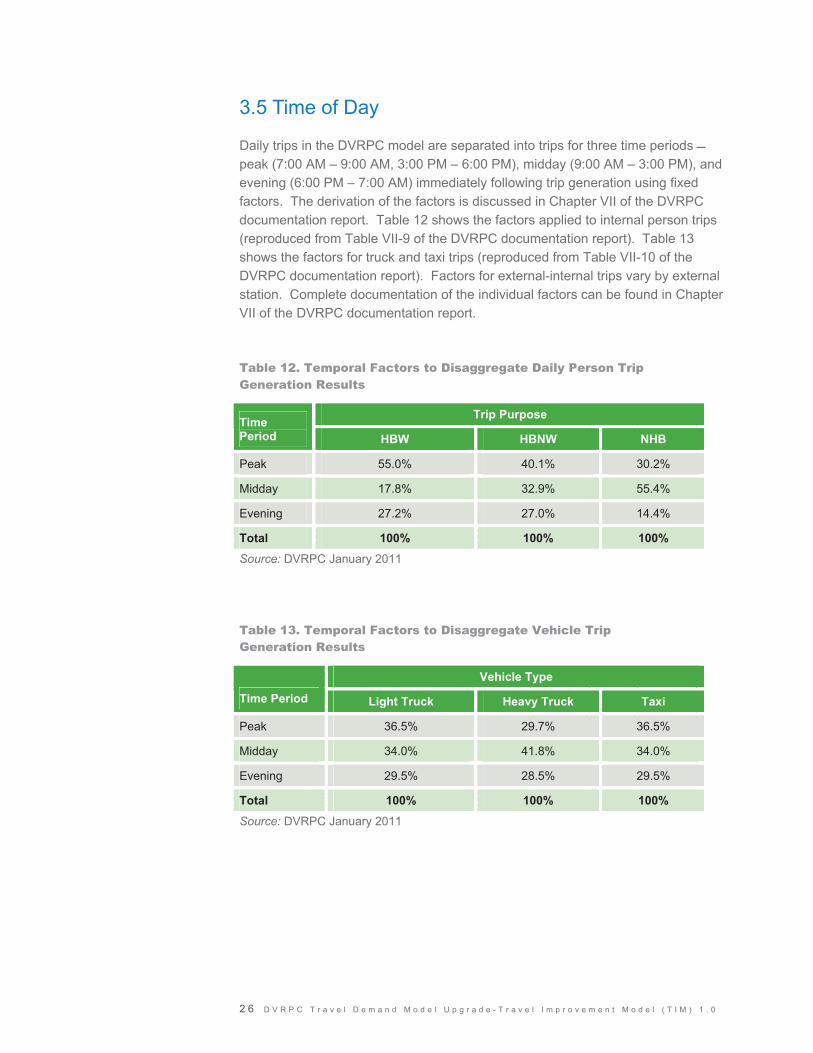
Daily trips in the DVRPC model are separated into trips for three time periods � peak (7:00 AM – 9:00 AM, 3:00 PM – 6:00 PM), midday (9:00 AM – 3:00 PM), and evening (6:00 PM – 7:00 AM) immediately following trip generation using fixed factors. The derivation of the factors is discussed in Chapter VII of the DVRPC documentation report. Table 12 shows the factors applied to internal person trips (reproduced from Table VII-9 of the DVRPC documentation report). Table 13 shows the factors for truck and taxi trips (reproduced from Table VII-10 of the DVRPC documentation report). Factors for external-internal trips vary by external station. Complete documentation of the individual factors can be found in Chapter VII of the DVRPC documentation report.
Table 12. Temporal Factors to Disaggregate Daily Person Trip Generation Results
Trip Purpose Time Period HBW HBNW NHB
Peak 55.0% 40.1% 30.2%
Midday 17.8% 32.9% 55.4%
Evening 27.2% 27.0% 14.4%
Total 100% 100% 100%
Source: DVRPC January 2011
Table 13. Temporal Factors to Disaggregate Vehicle Trip Generation Results
Vehicle Type
Time Period Light Truck Heavy Truck Taxi
Peak 36.5% 29.7% 36.5%
Midday 34.0% 41.8% 34.0%
Evening 29.5% 28.5% 29.5%
Total 100% 100% 100%
Source: DVRPC January 2011

D V R P C T r a v e l D e m a n d M o d e l U p g r a d e - T r a v e l I m p r o v e m e n t M o d e l ( T I M ) 1 . 0 2 7
3.6 Implementation
The trip generation process described above is implemented in VISUM through the use of a Python script. Trip generation is performed as part of the initial steps in the model and is not part of the feedback loop described in Chapter 7. The trip generation script is called by the master script for the VISUM model.
The mathematics of the Python script exactly match those used in the FORTRAN programs. The only difference is that the input for the four external-internal trip types is the highway distance in the VISUM model, rather than the airline distance used in the TRANPLAN model. For the internal person and vehicle trip purposes, the VISUM results exactly match those from the TRANPLAN model, except for miniscule rounding differences. For the external trip purposes, the results differ because of the different input variables, but the total number of trips for each purpose is the same, due to the normalizing of trips to the external station traffic count volumes.


D V R P C T r a v e l D e m a n d M o d e l U p g r a d e - T r a v e l I m p r o v e m e n t M o d e l ( T I M ) 1 . 0 2 9
C H A P T E R 4
Trip Distribution
DVRPC uses a gravity model formulation for trip distribution. The DVRPC model uses generalized highway cost as the impedance measure in the model. The impedance to travel from zone i to zone j is a combination of all the direct time and monetary elements encountered by trip makers. For travel by highway it includes in-vehicle travel time, out of vehicle time, parking charges, tolls, and direct vehicle operating costs.
4.1. Impedance
The impedance of travel from one zone to another by highway is determined by finding minimum impedance paths through the highway network (“skimming”), which is explained in a later section of this report. The impedance to travel by auto is defined for the DVRPC model as:
Imp_Hwy = 3.654 * OVT + 2.436 * IVT + 2.0 * Toll + 4.156 * Dist
where:
IVT = in-vehicle time (including network access time) in minutes
OVT = out-of-vehicle time (here: non-network terminal time) in minutes
Toll = auto toll in dollars
Dist = auto distance in miles
The impedance function used in trip distribution, however, is derived from the highway impedance above, but it uses a different scale. This different scale was used in TRANPLAN and has been replicated exactly in VISUM as follows:
ImpTD = 1.0*OVT + 0.666*IVT + 0.547*Toll + 1.137*Dist + 1.0*Penalty.
This rescaling is implemented in VISUM by multiplication of the impedance with a coefficient of 0.2736 in the trip distribution step of the VISUM model.
The variable penalty in the impedance formula is used as a kind of “k-factor” to adjust trip distribution on certain screen lines. Already in the TRANPLAN model, this type of penalty was used to represent the barrier of crossing the Delaware River, which is a state boundary, and to obtain reasonable crossing volumes. A

3 0 D V R P C T r a v e l D e m a n d M o d e l U p g r a d e - T r a v e l I m p r o v e m e n t M o d e l ( T I M ) 1 . 0
similar penalty was used to calibrate the amount of travel across the borders of the City of Philadelphia. Table 14 shows the trip distribution penalties as a county-to-county matrix.
Table 14. Trip Distribution Penalty Matrix
Destination County
Origin County B
ucks
Che
ster
t
Del
awar
e
Mon
tgom
ery
Phila
delp
hia
Bur
lingt
on
Cam
den
Glo
uces
ter
Mer
cer
Ber
ks
Exte
rnal
Bucks 2 2 2 2 2
Chester 2 2 2 2 2
Delaware 2 2 2 2 2
Montgomery 2 2 2 2 2
Philadelphia 2 2 2 2 1 1 1 1 2
Burlington 2 2 2 2 1 2
Camden 2 2 2 2 1 2
Gloucester 2 2 2 2 1 2
Mercer 2 2 2 2 1 2
Berks 2 2 2 2 2
External Source: DVRPC January 2011
The cost of travel by transit is included by the transit bias adjustment shown later in this section.
4.2. Gravity Model
The original TRANPLAN model used friction factors, based on the travel impedances, which were calibrated for each of the 10 internal and external person and vehicle trip purposes. These factors were not computed based on a continuous function, but instead used a piece-wise or “bin” function. VISUM requires that friction factors be computed based on one of several available functions, and so it was not possible to recreate the TRANPLAN friction factors. In VISUM the Box-Cox LOGIT functions were selected because they provided the closest fit to the average trip lengths from the TRANPLAN model, while also matching the overall travel patterns (e.g., county-to-county trips) reasonably close. In the case of some of the External-Internal demand strata, a flat LOGIT function
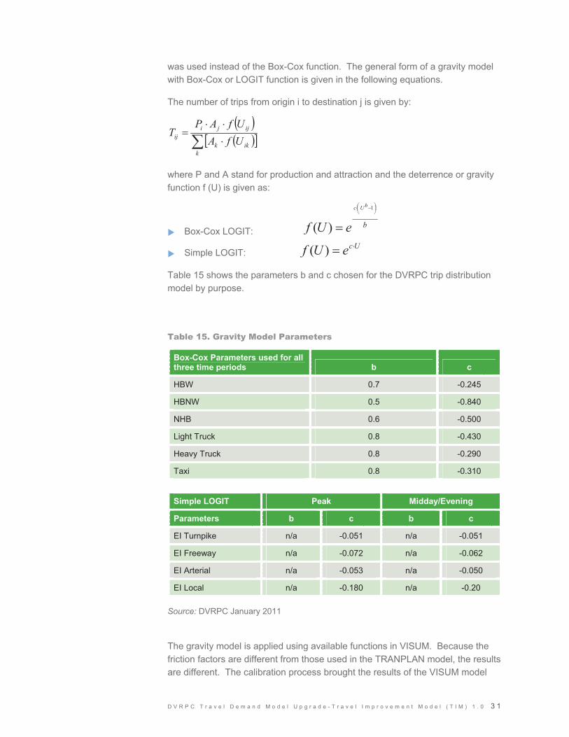
D V R P C T r a v e l D e m a n d M o d e l U p g r a d e - T r a v e l I m p r o v e m e n t M o d e l ( T I M ) 1 . 0 3 1
was used instead of the Box-Cox function. The general form of a gravity model with Box-Cox or LOGIT function is given in the following equations.
The number of trips from origin i to destination j is given by:
� �� �� �� �
��
kikk
ijjiij UfA
UfAPT
where P and A stand for production and attraction and the deterrence or gravity function f (U) is given as:
� Box-Cox LOGIT:
� Simple LOGIT:
Table 15 shows the parameters b and c chosen for the DVRPC trip distribution model by purpose.
Table 15. Gravity Model Parameters
Box-Cox Parameters used for all three time periods b c
HBW 0.7 -0.245
HBNW 0.5 -0.840
NHB 0.6 -0.500
Light Truck 0.8 -0.430
Heavy Truck 0.8 -0.290
Taxi 0.8 -0.310
Simple LOGIT Peak Midday/Evening
Parameters b c b c
EI Turnpike n/a -0.051 n/a -0.051
EI Freeway n/a -0.072 n/a -0.062
EI Arterial n/a -0.053 n/a -0.050
EI Local n/a -0.180 n/a -0.20
Source: DVRPC January 2011
The gravity model is applied using available functions in VISUM. Because the friction factors are different from those used in the TRANPLAN model, the results are different. The calibration process brought the results of the VISUM model
b
bUc
eUf��
�� ��
1
)(UceUf �)(

3 2 D V R P C T r a v e l D e m a n d M o d e l U p g r a d e - T r a v e l I m p r o v e m e n t M o d e l ( T I M ) 1 . 0
closer to those of the TRANPLAN model, but it was impossible to achieve a near-exact match. The results of the VISUM model, compared to those of the TRANPLAN model and observed survey data, are presented in Section 8.1.
4.3. Adjustment to Trip Distribution for Transit Service Quality
In the original TRANPLAN model, a correction procedure was used to adjust the trip distribution results for zone interchanges with good transit service since the trip distribution model does not consider the trip-inducing effect of transit mobility. Zone-to-zone pairs with good transit service have their number of trips increased, while zone-to-zone pairs with poor or no transit service have their number of trips decreased. This procedure, programmed in FORTAN in the TRANPLAN model, was coded into VISUM using a Python script.
The first step in adjusting the trip distribution results to account for the transit bias is to calculate the impedance difference between the highway and transit impedances, defined as:
ID[i,j] = Imp_Transit[i,j] / 2.43 – Imp_Hwy[i,j].
Imp_Hwy = highway impedance in minutes and is defined as:
Imp_Hwy = 1.0 * OVT + 2.436 * IVT + 2.0 * Toll + 4.156 * Dist
where:
IVT = highway in-vehicle time (including network access time) in minutes
Toll = auto toll in dollars
Dist = auto distance in miles
and Imp_Transit = transit impedance in minutes, and is defined as:
Imp_Transit = 7.31 * OVT + 2.436 * IVT + 14.6 * Fare + 29.23 * NT
where:
IVT = transit in-vehicle time in minutes
OVT = transit out of vehicle time in minutes
Fare = transit fare in dollars
NT = number of transit transfers
As the above formulas show, in computing the impedance difference (ID), the impedance scaling is not in line with other places in the model. In particular, transit impedance is divided by 2.43 to maintain consistency in units with the formula in the TRANPLAN version of the model. Also, in highway impedance, out
D V R P C T r a v e l D e m a n d M o d e l U p g r a d e - T r a v e l I m p r o v e m e n t M o d e l ( T I M ) 1 . 0 3 3
of vehicle time (OVT) does not use the same coefficient as in the rest of the model. This model was imported from the TRANPLAN model with few changes, but will be revisited by the use of logsum impedances for trip distribution in the next version of the model.
A positive impedance difference means that there is poor transit service, while a negative impedance difference means that the transit service between i and j is good. The impedance difference is used in the following equation to compute an adjustment factor (y):
y = 1.15 � 0.001(ID) 0.80 � y � 1.2.
The adjustment factor is held to a maximum value of 1.2 and a minimum value of 0.80. This factor shows the compensation needed to the trip interchange to account for the quality of transit service. The number of trips for each i -> j interchange and trip purpose as determined from the highway gravity model is multiplied by the adjustment factor to compensate for the impedance of travel by transit.


D V R P C T r a v e l D e m a n d M o d e l U p g r a d e - T r a v e l I m p r o v e m e n t M o d e l ( T I M ) 1 . 0 3 5
C H A P T E R 5
Mode Choice
The DVRPC mode choice process splits person trip tables for HBW, HBNW, and NHB into auto and transit trips. The mode choice process consists of several steps:
� Split mode captives from the total demand
� Split non-captive demand into 0-car households and 1+ car households
� Nested mode choice for six demand strata: HBW 0-car, HBNW 0-car, NHB 0-car, HBW 1+ car, HBNW 1+ car, NHB 1+ car
� Vehicle occupancy computation
Figure 4 illustrates DVRPC’s mode choice model and the individual steps.
Figure 4. DVRPC Mode Choice Model as Flow Chart
Demand Segment
Transit Captives
Highway Captives
“Choice Riders”
0 Car HH
1+ Car HH
Transit
Hwy Pers. Trips
Transit-Walk
Transit-Drive
Transit
Hwy Pers. Trips
Transit-Walk
Transit-Drive
Veh. Trips
Veh. Trips
Source: DVRPC January 2011
All four steps above are replications of the mode choice model in the previous TRANPLAN model. The most important difference from the TRANPLAN implementation occurs in the core choice model (step 3). In TRANPLAN, two flat binary LOGIT choice models were computed: highway vs. transit-walk-access and highway vs. transit-auto-access. Then the results of both choice models were averaged to obtain the final share of all three modes. The VISUM implementation performs only one nested logit mode choice model which computes the shares for all three modes. The parameters were deduced from corresponding TRANPLAN parameters and then adjusted during model calibration.
3 6 D V R P C T r a v e l D e m a n d M o d e l U p g r a d e - T r a v e l I m p r o v e m e n t M o d e l ( T I M ) 1 . 0
5.1 Supply Characteristics in Mode Choice
Several explanatory variables are included in the mode choice calculation. They can be divided into three groups: network-dependent supply characteristics, constant supply characteristics, and other constant inputs. The explanatory variables are listed below. Later in the chapter, when the individual components of DVRPC’s mode choice are described, references to these explanatory variables are made to explain how they impact the results.
Network-Dependent Variables - VISUM Skims
VISUM computes skims by averaging the travel conditions along multiple paths and averaging them for each origin-destination pair. The results are skim matrices, which are generated separately for highway, transit-walk, and transit-auto. The following skims are used in mode choice:
Imp_Hwy[i,j] = highway impedance, and defined as:
3.654 * OVT + 2.436 * IVT + 2.0 * Toll + 4.156 * Distance
where:
IVT = auto in-vehicle time (including network access time) in minutes
OVT = auto out of vehicle time in minutes2
Toll = auto toll in dollars
Distance = auto distance in miles
Imp_Transit[i,j] = transit impedance, and defined as:
7.31 * OVT + 2.436 * IVT + 14.6 * Fare + 29.23 * NT
where:
IVT = transit in-vehicle time in minutes
OVT = transit out of vehicle time in minutes
Fare = transit fare in dollars
NT = number of transit transfers
The average portion used by each transit submode for an origin-destination pair, measured as the portion of the in-vehicle distance traveled with the particular sub-mode and given as a number between 0.0 and 1.0:
2Auto OVT is not used in network skimming.
D V R P C T r a v e l D e m a n d M o d e l U p g r a d e - T r a v e l I m p r o v e m e n t M o d e l ( T I M ) 1 . 0 3 7
� CommuRail[i,j] – the average portion of total transit in-vehicle distance traveled on the regional rail transport systems (RRNJ and RRPA)
� HeavyRail[i,j] – the average portion of total transit in-vehicle distance traveled on the heavy rail transport systems (HRCty, HRVct)
� PATCORail[i,j] – the average portion of total vehicle distance traveled on the transport system PATCO
Constant Supply Characteristics
Two supply characteristics are not determined by network skimming. Instead they are defined outside of VISUM:
� TermTime[i,j] = highway terminal time in minutes, given as a matrix
� ParkingCost[i] in dollars
The derivation of these variables can be found in the DVRPC documentation report.
Other Constant Explanatory Variables
Finally, some variables that influence mode choice are not considered as transportation supply. Instead they represent other explanatory factors:
� CPA[i] = county planning area, the traffic analysis zone belongs to (used in the captivity model)
� AreaType[i] = DVRPC area type per traffic analysis zone (affects LU_Impfactor below)
� ModeChoicePenalty[i,j] = a penalty for certain OD pairs, included in nested mode choice
� “Impedance factor”, LU_ImpFactor[i,j] = a transit discount or penalty, in the TRANPLAN model referred to as the “impedance factor“; it simulates the impact of land use on transit demand and is a function of the area types of origin and destination zone. The impedance factor is directly included in the nested mode choice.
5.2 Mode Captives and Auto Ownership
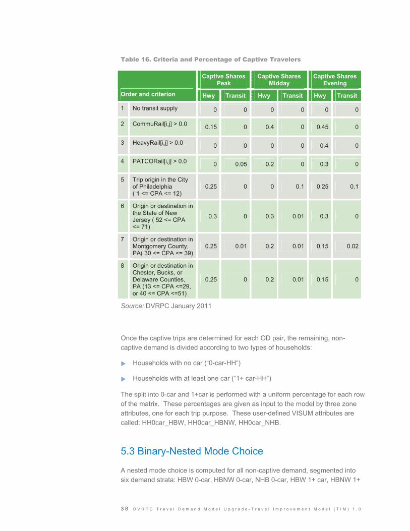
Captive travelers are split from the entire demand and stored in separate matrices for highway and transit. The captive shares, shown in Table 16, are differentiated by time of day, but are applied uniformly over all trip purposes. The resulting captive matrices “bypass” the mode choice and are added directly to the demand that is fed into the assignment.
3 8 D V R P C T r a v e l D e m a n d M o d e l U p g r a d e - T r a v e l I m p r o v e m e n t M o d e l ( T I M ) 1 . 0
Table 16. Criteria and Percentage of Captive Travelers
Source: DVRPC January 2011
Once the captive trips are determined for each OD pair, the remaining, non-captive demand is divided according to two types of households:
� Households with no car (“0-car-HH“)
� Households with at least one car (“1+ car-HH“)
The split into 0-car and 1+car is performed with a uniform percentage for each row of the matrix. These percentages are given as input to the model by three zone attributes, one for each trip purpose. These user-defined VISUM attributes are called: HH0car_HBW, HH0car_HBNW, HH0car_NHB.
5.3 Binary-Nested Mode Choice
A nested mode choice is computed for all non-captive demand, segmented into six demand strata: HBW 0-car, HBNW 0-car, NHB 0-car, HBW 1+ car, HBNW 1+
Captive Shares Peak
Captive Shares Midday
Captive Shares Evening
Order and criterion Hwy Transit Hwy Transit Hwy Transit
1 No transit supply 0 0 0 0 0 0
2 CommuRail[i,j] > 0.0 0.15 0 0.4 0 0.45 0
3 HeavyRail[i,j] > 0.0 0 0 0 0 0.4 0
4 PATCORail[i,j] > 0.0 0 0.05 0.2 0 0.3 0
5 Trip origin in the City of Philadelphia ( 1 <= CPA <= 12)
0.25 0 0 0.1 0.25 0.1
6 Origin or destination in the State of New Jersey ( 52 <= CPA <= 71)
0.3 0 0.3 0.01 0.3 0
7 Origin or destination in Montgomery County, PA( 30 <= CPA <= 39)
0.25 0.01 0.2 0.01 0.15 0.02
8 Origin or destination in Chester, Bucks, or Delaware Counties, PA (13 <= CPA <=29, or 40 <= CPA <=51)
0.25 0 0.2 0.01 0.15 0
D V R P C T r a v e l D e m a n d M o d e l U p g r a d e - T r a v e l I m p r o v e m e n t M o d e l ( T I M ) 1 . 0 3 9
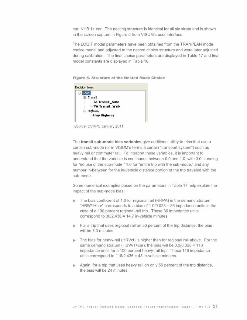
car, NHB 1+ car. The nesting structure is identical for all six strata and is shown in the screen capture in Figure 5 from VISUM’s user interface.
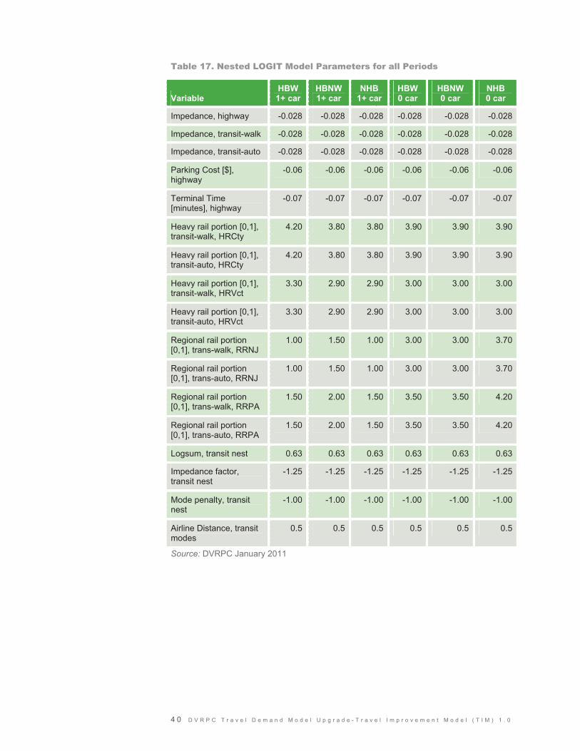
The LOGIT model parameters have been obtained from the TRANPLAN mode choice model and adjusted to the nested choice structure and were later adjusted during calibration. The final choice parameters are displayed in Table 17 and final model constants are displayed in Table 18.
Figure 5. Structure of the Nested Mode Choice
The transit sub-mode bias variables give additional utility to trips that use a certain sub-mode (or in VISUM’s terms a certain “transport system”) such as heavy rail or commuter rail. To interpret these variables, it is important to understand that the variable is continuous between 0.0 and 1.0, with 0.0 standing for “no use of the sub-mode,” 1.0 for “entire trip with the sub-mode,” and any number in-between for the in-vehicle distance portion of the trip traveled with the sub-mode.
Some numerical examples based on the parameters in Table 17 help explain the impact of the sub-mode bias:
� The bias coefficient of 1.0 for regional rail (RRPA) in the demand stratum “HBW/1+car” corresponds to a bias of 1.0/0.028 = 36 impedance units in the case of a 100 percent regional-rail trip. These 36 impedance units correspond to 36/2.436 = 14.7 in-vehicle minutes.
� For a trip that uses regional rail on 50 percent of the trip distance, the bias will be 7.3 minutes.
� The bias for heavy-rail (HRVct) is higher than for regional rail above. For the same demand stratum (HBW/1+car), the bias will be 3.3/0.028 = 118 impedance units for a 100 percent heavy-rail trip. These 118 impedance units correspond to 118/2.436 = 48 in-vehicle minutes.
� Again, for a trip that uses heavy rail on only 50 percent of the trip distance, the bias will be 24 minutes.
Source: DVRPC January 2011
4 0 D V R P C T r a v e l D e m a n d M o d e l U p g r a d e - T r a v e l I m p r o v e m e n t M o d e l ( T I M ) 1 . 0
Table 17. Nested LOGIT Model Parameters for all Periods
Variable HBW1+ car
HBNW1+ car
NHB 1+ car
HBW 0 car
HBNW 0 car
NHB 0 car
Impedance, highway -0.028 -0.028 -0.028 -0.028 -0.028 -0.028
Impedance, transit-walk -0.028 -0.028 -0.028 -0.028 -0.028 -0.028
Impedance, transit-auto -0.028 -0.028 -0.028 -0.028 -0.028 -0.028
Parking Cost [$], highway
-0.06 -0.06 -0.06 -0.06 -0.06 -0.06
Terminal Time [minutes], highway
-0.07 -0.07 -0.07 -0.07 -0.07 -0.07
Heavy rail portion [0,1], transit-walk, HRCty
4.20 3.80 3.80 3.90 3.90 3.90
Heavy rail portion [0,1], transit-auto, HRCty
4.20 3.80 3.80 3.90 3.90 3.90
Heavy rail portion [0,1], transit-walk, HRVct
3.30 2.90 2.90 3.00 3.00 3.00
Heavy rail portion [0,1], transit-auto, HRVct
3.30 2.90 2.90 3.00 3.00 3.00
Regional rail portion [0,1], trans-walk, RRNJ
1.00 1.50 1.00 3.00 3.00 3.70
Regional rail portion [0,1], trans-auto, RRNJ
1.00 1.50 1.00 3.00 3.00 3.70
Regional rail portion [0,1], trans-walk, RRPA
1.50 2.00 1.50 3.50 3.50 4.20
Regional rail portion [0,1], trans-auto, RRPA
1.50 2.00 1.50 3.50 3.50 4.20
Logsum, transit nest 0.63 0.63 0.63 0.63 0.63 0.63
Impedance factor, transit nest
-1.25 -1.25 -1.25 -1.25 -1.25 -1.25
Mode penalty, transit nest
-1.00 -1.00 -1.00 -1.00 -1.00 -1.00
Airline Distance, transit modes
0.5 0.5 0.5 0.5 0.5 0.5
Source: DVRPC January 2011

D V R P C T r a v e l D e m a n d M o d e l U p g r a d e - T r a v e l I m p r o v e m e n t M o d e l ( T I M ) 1 . 0 4 1
Table 18. Nested LOGIT Model Constants for all Periods
Variable HBW1+ car
HBNW1+ car
NHB1+ car
HBW 0 car
HBNW0 car
NHB 0 car
Constant, highway
(all periods)
0.00 0.00 0.00 0.00 0.00 0.00
Constant, transit-walk, PK -9.0 -10.5 -12.5 -7.5 -9.0 -12.5
Constant, transit-walk, MD -8.8 -10.4 -12.4 -7.4 -9.4 -12.4
Constant, transit-walk, EV -9.2 -10.7 -12.7 -7.7 -9.7 -12.7
Constant, transit-auto, PK -7.7 -7.7 -7.7 -6.1 -6.8 -6.2
Constant, transit-auto, MD -7.5 -7.5 -7.7 -4.7 -6.5 -6.9
Constant, transit-auto, EV -7.4 -7.4 -7.6 -5.9 -6.7 -7.0
Source: DVRPC January 2011
As previously mentioned, there are two correction variables in the mode choice model, “impedance factor” and “mode penalty.” Both are constant in the sense that they do not depend on supply changes modeled in the network. “Impedance factor” has been replicated exactly as used in the TRANPLAN model. “Mode penalty” is a result of model calibration but has been used to a lesser extent than in the TRANPLAN model. For both parameters, positive values bias the results towards the highway mode. Tables 19 and 20 display the values used in the VISUM model for both correction variables.
Another variable in the transit utility is the airline distance of the trip. This variable increases utility of transit the longer the trip is. It was added to the model since the original mode choice had produced transit trips that were too short across all transit submodes.
While the very first VISUM translation of the model used different scales for highway and transit impedance, this discrepancy has been fixed so that the model is consistent in terms of in-vehicle time units:
Imp_tran = 7.31 * OVT + 2.436 * IVT + 14.6 * Fare + 29.23 * NT
Imp_hwy = 3.654 * OVT + 2.436 * IVT + 2.0 * Toll + 4.156 *Distance

4 2 D V R P C T r a v e l D e m a n d M o d e l U p g r a d e - T r a v e l I m p r o v e m e n t M o d e l ( T I M ) 1 . 0
Table 19. Mode Choice Correction Variable "Impedance Factor"
Area type of the destination zone
Region Type 1 –
CBD 2 – CBD Fringe
3 – Urban
4 – Suburban
5 – Rural
6 – Open Rural
1 – CBD 0.0 0.0 -4.5 0.0 0.0 0.0
2 – CBD Fringe 0.0 0.0 -1.5 0.0 0.0 0.0
3 – Urban -5.0 -5.0 -1.5 3.0 3.0 3.0
4 – Suburban -4.0 -4.0 0.5 10.0 10.0 10.0
5 – Rural -4.0 -4.0 0.5 10.0 10.0 10.0
Area type of the origin zone
6 – Open Rural -4.0 -4.0 0.5 10.0 10.0 10.0
Source: DVRPC January 2011
Table 20. Mode Choice Penalty Matrix
Destination County
Origin County B
ucks
Che
ster
Del
awar
e
Mon
tgom
ery
Phila
delp
hia
Bur
lingt
on
Cam
den
Glo
uces
ter
Mer
cer
Ber
ks
Exte
rnal
Bucks 2 2 4
Chester 2 4 2
Delaware 2 4 4
Montgomery 4 4
Philadelphia
Burlington 4 2 2
Camden 4 2
Gloucester 2 4
Mercer 4 4 4 4 3
Berks
External Source: DVRPC January 2011

D V R P C T r a v e l D e m a n d M o d e l U p g r a d e - T r a v e l I m p r o v e m e n t M o d e l ( T I M ) 1 . 0 4 3
5.4 Vehicle Occupancy
The vehicle occupancy rate is defined as the number of persons per car and is computed according to the following formula:
Occupancy rate = minimum (A + B * Imp_Hwy; C)
Vehicle trips = person trips/occupancy
In the occupancy model, neither terminal time nor parking cost is included in the highway impedance.
The parameters A, B, and C are very similar to the ones used in the TRANPLAN model, except that the parameter B has been scaled to impedance units. This is a slight change from the TRANPLAN model which used only highway in-vehicle time in the vehicle occupancy model. The parameters are shown in Table 21. The resulting occupancy rates per OD pair are applied to both captive and non-captive highway person trips. As a result, vehicle trips are obtained and are input to highway assignment.
Table 21. Coefficients of the Vehicle Occupancy Model
Time Period Purpose A B C
HBW 1.012 0.0010 n/a
HBNW 1.539 0.0033 2.5
Peak
NHB 1.290 0.0000 n/a
HBW 1.000 0.0012 n/a
HBNW 1.210 0.0035 2.5
Midday
NHB 1.230 0.0000 n/a
HBW 1.012 0.0012 n/a
HBNW 1.430 0.0045 2.5
Evening
NHB 1.350 0.0000 n/a
Source: DVRPC January 2011

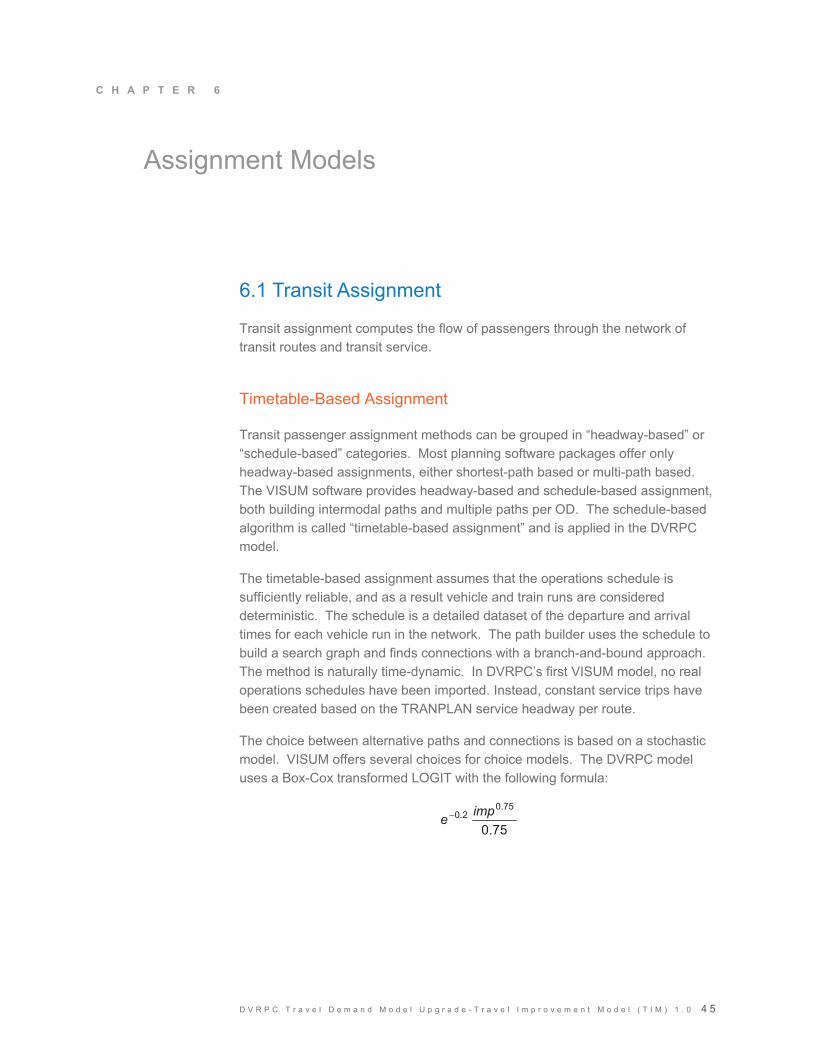
D V R P C T r a v e l D e m a n d M o d e l U p g r a d e - T r a v e l I m p r o v e m e n t M o d e l ( T I M ) 1 . 0 4 5
C H A P T E R 6
Assignment Models
6.1 Transit Assignment
Transit assignment computes the flow of passengers through the network of transit routes and transit service.
Timetable-Based Assignment
Transit passenger assignment methods can be grouped in “headway-based” or “schedule-based” categories. Most planning software packages offer only headway-based assignments, either shortest-path based or multi-path based. The VISUM software provides headway-based and schedule-based assignment, both building intermodal paths and multiple paths per OD. The schedule-based algorithm is called “timetable-based assignment” and is applied in the DVRPC model.
The timetable-based assignment assumes that the operations schedule is sufficiently reliable, and as a result vehicle and train runs are considered deterministic. The schedule is a detailed dataset of the departure and arrival times for each vehicle run in the network. The path builder uses the schedule to build a search graph and finds connections with a branch-and-bound approach. The method is naturally time-dynamic. In DVRPC’s first VISUM model, no real operations schedules have been imported. Instead, constant service trips have been created based on the TRANPLAN service headway per route.
The choice between alternative paths and connections is based on a stochastic model. VISUM offers several choices for choice models. The DVRPC model uses a Box-Cox transformed LOGIT with the following formula:
75.0
75.02.0 impe �

4 6 D V R P C T r a v e l D e m a n d M o d e l U p g r a d e - T r a v e l I m p r o v e m e n t M o d e l ( T I M ) 1 . 0
Impedance
In VISUM’s transit assignment and skimming procedures, the impedance function
has been rescaled to minutes of in-vehicle time as follows:
Imp_tran = 3.0 * OVT + 1.0 * IVT + 6.0 * Fare + 12.0 * NT.
The OVT (out-of-vehicle time) includes:
Access/egress time;
Walk time at transfer; and
Wait time, computed as 50 percent of the service headway at boarding
VISUM Transit Assignment Impedance settings are shown in Figure 6 below.
Figure 6. Transit Assignment Impedance Settings
Source: DVRPC January 2011
D V R P C T r a v e l D e m a n d M o d e l U p g r a d e - T r a v e l I m p r o v e m e n t M o d e l ( T I M ) 1 . 0 4 7
6.2 Transit Skimming
Level-of-service matrices for transit are computed only once at the very beginning of the model run, as they do not depend on network volumes. An extension of the model for future forecasts includes an update of the skims during the feedback loop.
In VISUM, the value for one OD pair in all skim matrices does represent the average over all paths used for the particular OD pair.
It should be noted that the transit runtime does not depend on highway link speeds for the 2005 case. For future networks, an automated adjustment routine has been set up which recomputes transit runtimes as a function of changes in highway link speeds.
All level of service indicators represent the weighted average conditions over all paths of a particular OD pair. The following transit level-of-service indicators are skimmed for use in mode choice:
� Impedance (according to the above formula)
� Percent In-vehicle distance for HRCty � [0,1]
� Percent In-vehicle distance for HRVct � [0,1]
� Percent In-vehicle distance for PATCO � [0,1]
� Percent In-vehicle distance for RRNJ � [0,1]
� Percent In-vehicle distance for RRPA � [0,1]
6.3 Highway Assignment
The highway assignment step computes vehicle flow over all the street network. In the following section all the components of the highway assignment are explained. The applied algorithm is VISUM's path-based equilibrium assignment method, set up as a single-class assignment, i.e., with one single matrix representing all vehicle trips. Other inputs are the highway network model, which was explained earlier and the impedance and delay models.
Vehicle Trip Matrix for Assignment
The OD demand matrix, which is used in highway assignment, is composed of several components, mainly results of trip distribution, mode choice, or the vehicle occupancy model. The total demand is made symmetric before assignment. Table 22 shows all the components that are summed up in each time period and the total number of vehicle trips that each component contributes.

�
# 8 � � � � � � � � � � � � � � � � � � � � � � � � � � � � � � � � � � � � � � � � � � � � � � � � � � � � � � � � � � � � � � � � � ! �
�������������������������������������������
�
Mat
rix N
umbe
r M
atrix
Nam
e PK
M
D
EV
24-H
%
of t
otal
1002
hb
w_1
+car
_hw
_veh
1,
404,
715
443,
213
637,
203
2,48
5,13
113
.0%
1022
hb
w_0
car_
hw_v
eh
92,8
7628
,835
36
,952
158,
663
0.8%
1032
hb
w_c
apt_
hw_v
eh
470,
081
164,
961
284,
837
919,
879
4.8%
1042
hb
nw_1
+car
_hw
_veh
1,
943,
854
1,99
6,83
9 1,
311,
673
5,25
2,36
627
.4%
1062
hb
nw_0
car_
hw_v
eh
66,5
2667
,816
38
,176
172,
518
0.9%
1072
hb
nw_c
apt_
hw_v
eh
642,
005
607,
264
453,
739
1,70
3.00
88.
9%
1082
nh
b_1+
car_
hw_v
eh
834,
359
1,56
3,12
1 37
3,88
72,
771,
367
14.5
%
1102
nh
b_0c
ar_h
w_v
eh
43,7
9582
,179
19
,659
145,
633
0.8%
1112
nh
b_ca
pt_h
w_v
eh
262,
745
481,
679
141,
284
885,
708
4.6%
1510
L_
Truc
k 77
6,00
372
1,45
3 63
0,36
32,
127,
819
11.1
%
1520
H
_Tru
ck
355,
826
492,
419
341,
061
1,18
9,30
66.
2%
1530
Ta
xi
47,0
1243
,792
37
,996
128,
800
0.7%
1551
E
I_tp
k 45
,083
44,7
44
54,9
6614
4,79
30.
8%
1552
E
I_fre
e 90
,935
82,9
09
85,8
4325
9,68
71.
4%
1553
E
I_ar
t 19
1,51
616
9,42
0 15
8,82
551
9,76
12.
7%
1554
E
I_lo
c 46
,764
36,3
33
35,6
6911
8,76
60.
6%
1600
E
E H
wy
60,2
2262
,037
60
,222
182,
481
1.0%
2000
To
tal V
ehic
le T
rips
7,37
4,31
77,
089,
014
4,70
2,35
519
,165
,686
100%
Tab
le 2
2. C
ompo
siti
on o
f th
e T
otal
Hig
hway
Dem
and
as V
ehic
le T
rips
Sou
rce:
DV
RP
C �
����
���
��
D V R P C T r a v e l D e m a n d M o d e l U p g r a d e - T r a v e l I m p r o v e m e n t M o d e l ( T I M ) 1 . 0 4 9
Path-Based User-Equilibrium Assignment Method
VISUM’s path-based assignment is organized in an outer loop and an inner loop. The outer loop computes a shortest path search for all OD pairs, adds the found shortest paths to the path set, and then performs several rounds of inner loops. The inner loop, also referred to as “balancing steps,” goes over all OD pairs and shifts demand between the alternative paths until every path of the OD pairs enjoys the same travel time. Travel times for all links are updated immediately after each shift of demand. The algorithm terminates when the user equilibrium is given for all OD pairs. Two different measures are used to define equilibrium – relative gap, a measure of closeness to the optimal cost solution which the assignment algorithm is trying to maximize, or when a maximal deviation of impedances between alternate paths for the same OD pair is not exceeded. The algorithm can also terminate when a maximum number of iterations of the inner and the outer loops is reached. The algorithm terminates when the first of these three criteria are met (max. impedance difference for alternate paths for an OD pair, max. relative gap, max. number of iterations).
The user parameters of the algorithm, as shown in Figure 7, have been chosen for the DVRPC model with the goal to obtain fast convergence in the context of a combined equilibrium:
� Acceptable gaps:
� The acceptable impedance difference between alternate paths at the OD level (“permitted deviation”) is set to zero difference between alternative paths, which means that this criterion will not be effective with the exception of a perfect equilibrium with zero gap everywhere.
� System level gap (“max. rel. gap”) is set to 0.0001 = 1.0E-4
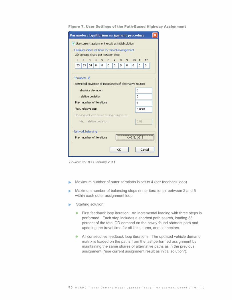
5 0 D V R P C T r a v e l D e m a n d M o d e l U p g r a d e - T r a v e l I m p r o v e m e n t M o d e l ( T I M ) 1 . 0
Figure 7. User Settings of the Path-Based Highway Assignment
� Maximum number of outer iterations is set to 4 (per feedback loop)
� Maximum number of balancing steps (inner iterations): between 2 and 5 within each outer assignment loop
� Starting solution:
� First feedback loop iteration: An incremental loading with three steps is performed. Each step includes a shortest path search, loading 33 percent of the total OD demand on the newly found shortest path and updating the travel time for all links, turns, and connectors.
� All consecutive feedback loop iterations: The updated vehicle demand matrix is loaded on the paths from the last performed assignment by maintaining the same shares of alternative paths as in the previous assignment (“use current assignment result as initial solution”).
Source: DVRPC January 2011

D V R P C T r a v e l D e m a n d M o d e l U p g r a d e - T r a v e l I m p r o v e m e n t M o d e l ( T I M ) 1 . 0 5 1
Network Objects with Constraints and Delays to Highway Travel
VISUM allows links, turns, and connectors to contribute to path choice and travel time with attributes such as free-flow speed or time, capacity, and prohibitions for certain transport systems. In the current DVRPC model, these three network object classes contribute as follows to the travel conditions:
� Links: capacity-constraint travel speed
� Turns: no restrictions no delays
� Connectors: constant travel times, not dependent of volume
Link Capacity Model
Following the same approach as the TRANPLAN model, base capacity is given as a daily capacity in the user-defined link attribute “CAP_24H”. The time-of-day capacities are derived as percentages of daily capacity. The percentage represents the duration of the assignment period and the degree of “peaking” during the period. The following factors are applied:
� Peak period (duration 3+2 hours): capacity = 30% x CAP_24H
� Midday period (duration 6 hours): capacity = 34% x CAP_24H
� Evening period (duration 13 hours): capacity = 48% x CAP_24H
Impedance Function
The DVRPC highway impedance function is defined as:
Imp_hwy = 3.654 * OVT + 2.436 * IVT + 2.0 * Toll + 4.156 * Dist
With units: minutes, dollar, miles
During the actual highway skimming step, the impedance function is scaled up. This is to account for internal rounding in the VISUM software as not all units are stored to true floating point precision. This helps to account for different units and ensures best convergence behavior with high impedance values:
100.0 IVT + 4926.0 Toll + 10.236 Dist
With units: seconds and 1/1000 miles
The impedance is factored back down to the previously displayed version shown above with coefficient 2.436 for IVT, which is compliant with DVRPC’s model documentation. The scale factor is 0.000406 = 2.436 / (100 * 60).

5 2 D V R P C T r a v e l D e m a n d M o d e l U p g r a d e - T r a v e l I m p r o v e m e n t M o d e l ( T I M ) 1 . 0
Volume-Delay Functions
Three different volume-delay functions are applied as follows:
� For most links, a BPR function is used with the following parameters: t = t0 * (1 + 0.15 * (v/c)7)
� Constant travel time for so called dummy links (link types 90, 94--99)
� Toll plaza function with three different parameter sets for link types 91, 92, and 93
The Toll Plaza Delay Function
DVRPC uses a hyperbolic delay function for toll plazas, which models three kinds of delays: deceleration in approach to the plaza, queuing, and acceleration after the plaza. The original “Florida Turnpike VDF” in TRANPLAN has been mathematically transformed and streamlined for VISUM.
The VISUM function has the following form:
���
�
���
�
�
����
� �
� ���
��
�
��
SatCritcapvol
capvoldSatCritd
Satcritb
SatCritcapvol
capvol
b
av
av
tcur
1
1
1
'00
where several parameters of the function can be set in VISUM:
a = acceleration rate (mph/sec), example a = 2.5
a‘ = deceleration rate (mph/sec), example a‘= 5.5
b = service time (sec/car), example b = 6s
SatCrit = critical vol/cap ratio, example = 0.95
d = slope of linear extension, example d = 900 sec per 100% v/c
v0 = free flow speed
The new toll plaza function is implemented as a DLL file which needs to be included in the VISUM file set before starting the software.
In the DVRPC model, three VISUM link types, 91, 92, and 93 have been introduced for toll plazas with three specific parameter sets for the toll plaza volume delay function (VDF), as shown in Table 23 and Figure 8.
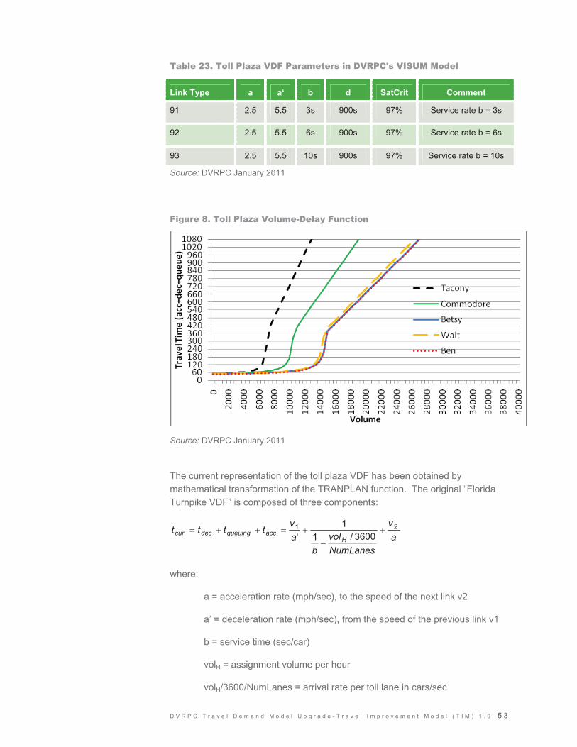
D V R P C T r a v e l D e m a n d M o d e l U p g r a d e - T r a v e l I m p r o v e m e n t M o d e l ( T I M ) 1 . 0 5 3
Table 23. Toll Plaza VDF Parameters in DVRPC's VISUM Model
Link Type a a‘ b d SatCrit Comment
91 2.5 5.5 3s 900s 97% Service rate b = 3s
92 2.5 5.5 6s 900s 97% Service rate b = 6s
93 2.5 5.5 10s 900s 97% Service rate b = 10s
Source: DVRPC January 2011
Figure 8. Toll Plaza Volume-Delay Function
Source: DVRPC January 2011
The current representation of the toll plaza VDF has been obtained by mathematical transformation of the TRANPLAN function. The original “Florida Turnpike VDF” is composed of three components:
av
NumLanesvol
bav
ttttH
accqueuingdeccur21
3600/11
'�
����
where:
a = acceleration rate (mph/sec), to the speed of the next link v2
a’ = deceleration rate (mph/sec), from the speed of the previous link v1
b = service time (sec/car)
volH = assignment volume per hour
volH/3600/NumLanes = arrival rate per toll lane in cars/sec
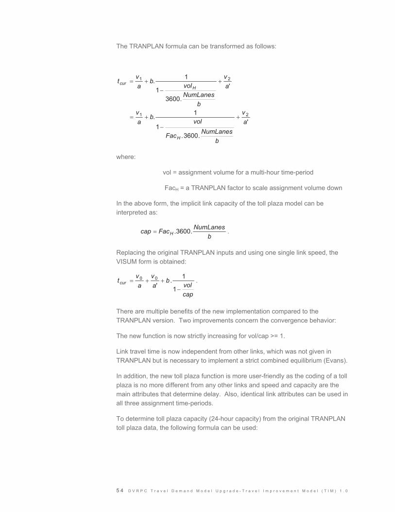
5 4 D V R P C T r a v e l D e m a n d M o d e l U p g r a d e - T r a v e l I m p r o v e m e n t M o d e l ( T I M ) 1 . 0
The TRANPLAN formula can be transformed as follows:
'
.3600.1
1.
'
.36001
1.
21
21
av
bNumLanesFac
volb
av
av
bNumLanesvol
bav
t
H
Hcur
�
�
�
��
�
where:
vol = assignment volume for a multi-hour time-period
FacH = a TRANPLAN factor to scale assignment volume down
In the above form, the implicit link capacity of the toll plaza model can be interpreted as:
b
NumLanesFaccap H .3600. .
Replacing the original TRANPLAN inputs and using one single link speed, the VISUM form is obtained:
capvol
bav
av
tcur�
��1
1.'00 .
There are multiple benefits of the new implementation compared to the TRANPLAN version. Two improvements concern the convergence behavior:
The new function is now strictly increasing for vol/cap >= 1.
Link travel time is now independent from other links, which was not given in TRANPLAN but is necessary to implement a strict combined equilibrium (Evans).
In addition, the new toll plaza function is more user-friendly as the coding of a toll plaza is no more different from any other links and speed and capacity are the main attributes that determine delay. Also, identical link attributes can be used in all three assignment time-periods.
To determine toll plaza capacity (24-hour capacity) from the original TRANPLAN toll plaza data, the following formula can be used:

D V R P C T r a v e l D e m a n d M o d e l U p g r a d e - T r a v e l I m p r o v e m e n t M o d e l ( T I M ) 1 . 0 5 5
lH
lll Fac
bNumLanesCONFACHCap
,
/360024_
��
where:
b = service rate
l = toll plaza link
CONFAC = TRANPLAN factor from period to 24H
6.4 Highway Skimming
In each feedback loop iteration, VISUM computes four matrices with level-of-service indicators:
� Composite impedance for use in trip distribution and mode choice
� Travel time in minutes, toll in dollars, and distance in miles
Notable details:
� In VISUM, the value for one OD pair in all skim matrices does represent the average overall paths used for the particular OD pair.
� The impedance is scaled down before it gets used in trip distribution and mode choice with a factor of 0.000406. This factor is derived as 2.436/(100 * 60) and takes into account that during assignment, the impedance is inflated by 100 and also that the time unit is in seconds. As a result, after scaling, the impedance numbers in the highway impedance matrix exactly match the DVRPC formula:
Imp_hwy = 3.654 * OVT + 2.436 * IVT + 2.0 * Toll + 4.156 * Dist
where:
IVT = auto in-vehicle time in minutes
OVT = auto out-of-vehicle time (terminal time) in minutes
Toll = auto toll in dollars
Distance = auto distance in miles

D V R P C T r a v e l D e m a n d M o d e l U p g r a d e - T r a v e l I m p r o v e m e n t M o d e l ( T I M ) 1 . 0 5 7
C H A P T E R 7
Combined Equilibrium
The objective of a combined equilibrium model is to obtain user optimal travel time and travel cost for the entire model system including distribution, mode choice, and assignment. One example for a combined equilibrium approach is the Evans approach. It is mathematically difficult to implement Evans for a complex metropolitan planning model. In particular, the exact Evans method can not be implemented with fast-converging contemporary highway assignment methods, such as VISUM’s path-based equilibrium method or VISUM’s origin-based LUCE algorithm.
In this context, the new DVRPC model has been set up with a feedback approach, which averages the impedance matrix between consecutive model iterations. The goal of the feedback and averaging is that the entire model converges quickly to a solution, where the travel impedance obtained as an output of the assignment is equal to the impedance which had been used as input for trip distribution and model choice.
7.1 Averaging of the Highway Impedance Matrix
From a model design point-of-view, there are three choices in terms of what to average in the feedback loop:
� Highway link volumes: Averaging of link volumes is common practice among U.S. MPOs. While it is easy to implement as an extension of Frank-Wolfe assignments, it is less intuitive with path- and origin-based assignment methods. Also, there are theoretical objections in the case of a multi-class assignment. Under the VISUM platform, link flow averaging has the disadvantage that some functionality for assignment evaluation would not be supported for averaged link volumes.
� Trip tables: While averaging of trip matrices is convenient for simple models, it is not for complex models because of extensive storage of matrices for each mode in each demand stratum. For the current TIM 1.0 model, more than 30 additional matrices would have to be managed for this method.

5 8 D V R P C T r a v e l D e m a n d M o d e l U p g r a d e - T r a v e l I m p r o v e m e n t M o d e l ( T I M ) 1 . 0
� Impedance matrices: A final method is the averaging of impedance matrices. It was decided to use this method for theoretical and practical reasons. For the 2005 model, only one matrix, highway impedance, is averaged and stored between iterations. For future model improvements, additional matrices might have to be averaged: transit impedance that depends on highway congestion or highway impedance separated for different modes, such as SOV, HOV, and truck.
7.2 Organization of the Feedback Loop
Figure 9 shows the organization of the model steps with feedback and averaging of impedance matrix. Note that the “warmstart” is not typically part of a normal model run. It can, however, be included for quick tests of scenarios, as it can significantly reduce the total computation time.
7.3 Predefined Averaging Weights
The impedance matrix is recomputed in each feedback iteration as an average of the newly skimmed impedance and the averaged impedance of the last iteration. The averaging method itself is based on predefined weights. The model scripts are set up to allow for two averaging methods to be used:
� Constant weights(CW): one given weight is applied in all iterations as follows:
AvgImp(n) = AvgImp(n-1) x weight + SkimImp(n) x (1 - weight)
� Method of successive averages (MSA), where the weights depend as follows:
AvgImp(n) = AvgImp(n-1) * (n-1)/n + SkimImp(n) * (1/n)
7.4 Convergence Monitoring and Loop Termination
Three statistics have been used to monitor model convergence. Also, the model run is set up so that these same three statistics can be used to terminate the model run, once sufficient convergence has been achieved:
� Relative Gap – to measure convergence of the highway assignment
� %RMSE impedance, comparing AvgImp(n) versus AvgImp(n-1) over all OD pairs – to measure convergence of the impedance matrix
� %RMSE trip matrix, comparing VehTrips(n) versus VehTrips(n-1) over all OD pairs – to measure convergence of the travel demand model
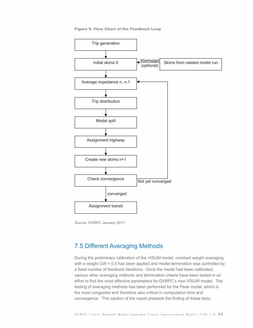
D V R P C T r a v e l D e m a n d M o d e l U p g r a d e - T r a v e l I m p r o v e m e n t M o d e l ( T I M ) 1 . 0 5 9
Figure 9. Flow Chart of the Feedback Loop
Source: DVRPC January 2011
7.5 Different Averaging Methods
During the preliminary calibration of the VISUM model, constant weight averaging with a weight CW = 0.5 has been applied and model termination was controlled by a fixed number of feedback iterations. Once the model had been calibrated, various other averaging methods and termination criteria have been tested in an effort to find the most effective parameters for DVRPC’s new VISUM model. The testing of averaging methods has been performed for the Peak model, which is the most congested and therefore also critical in computation time and convergence. This section of the report presents the finding of these tests.
Trip generation
Initial skims 0 Skims from related model run
Average impedance n, n-1
Modal split
Trip distribution
Assignment highway
Create new skims n+1
Check convergence
Assignment transit
Warmstart (optional)
Not yet converged
converged
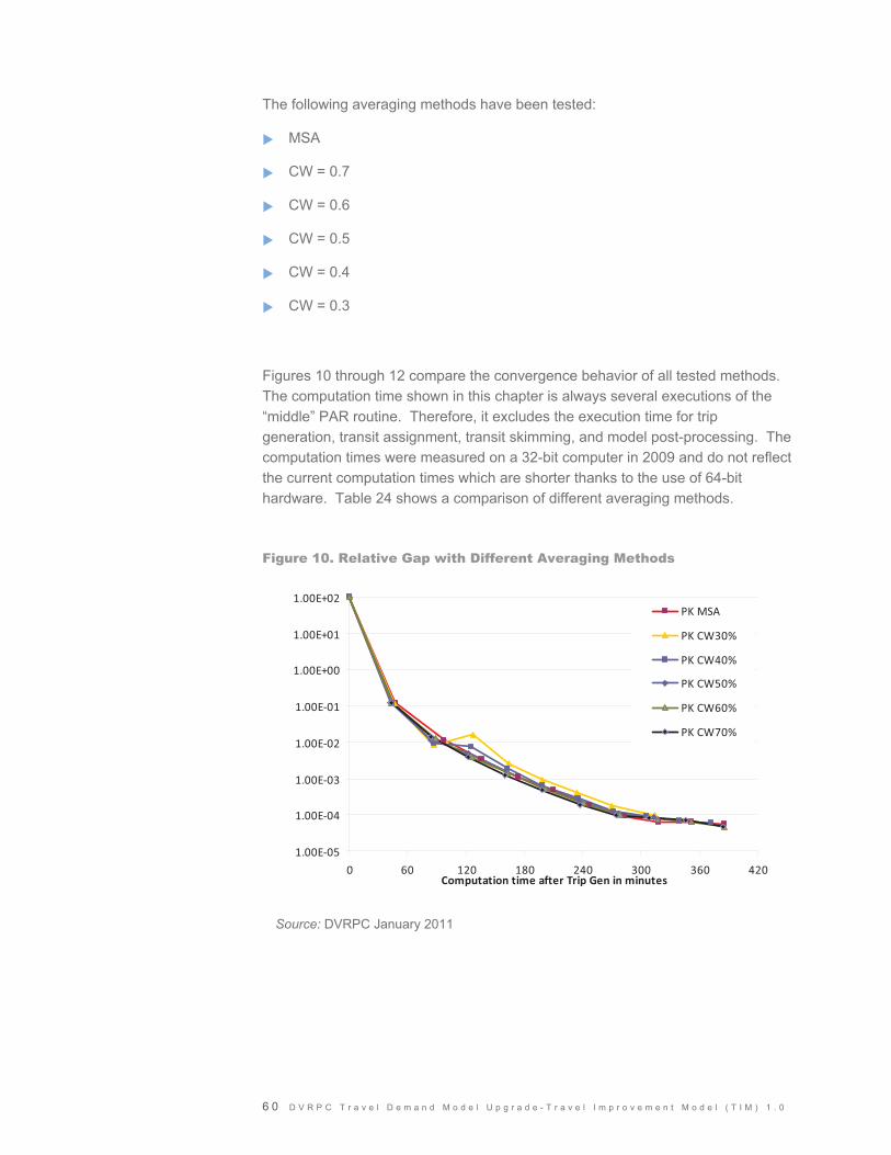
6 0 D V R P C T r a v e l D e m a n d M o d e l U p g r a d e - T r a v e l I m p r o v e m e n t M o d e l ( T I M ) 1 . 0
The following averaging methods have been tested:
� MSA
� CW = 0.7
� CW = 0.6
� CW = 0.5
� CW = 0.4
� CW = 0.3
Figures 10 through 12 compare the convergence behavior of all tested methods. The computation time shown in this chapter is always several executions of the “middle” PAR routine. Therefore, it excludes the execution time for trip generation, transit assignment, transit skimming, and model post-processing. The computation times were measured on a 32-bit computer in 2009 and do not reflect the current computation times which are shorter thanks to the use of 64-bit hardware. Table 24 shows a comparison of different averaging methods.
Figure 10. Relative Gap with Different Averaging Methods
1.00E�05
1.00E�04
1.00E�03
1.00E�02
1.00E�01
1.00E+00
1.00E+01
1.00E+02
0 60 120 180 240 300 360 420Computation�time�after�Trip�Gen�in�minutes
PK�MSA
PK�CW30%
PK�CW40%
PK�CW50%
PK�CW60%
PK�CW70%
Source: DVRPC January 2011

D V R P C T r a v e l D e m a n d M o d e l U p g r a d e - T r a v e l I m p r o v e m e n t M o d e l ( T I M ) 1 . 0 6 1
Figure 11. %RMSE-Demand with Different Averaging Methods
1.00E�01
1.00E+00
1.00E+01
1.00E+02
1.00E+03
1.00E+04
0 60 120 180 240 300 360 420Computation�time�after�Trip�Gen�in�minutes
PK�MSA
PK�CW30%
PK�CW40%
PK�CW50%
PK�CW60%
PK�CW70%
Source: DVRPC January 2011
Figure 12. %RMSE-Impedance with Different Averaging Methods
1.00E�02
1.00E�01
1.00E+00
1.00E+01
1.00E+02
1.00E+03
1.00E+04
0 60 120 180 240 300 360 420Computation�time�after�Trip�Gen�in�minutes
PK�MSA
PK�CW30%
PK�CW40%
PK�CW50%
PK�CW60%
PK�CW70%
Source: DVRPC January 2011
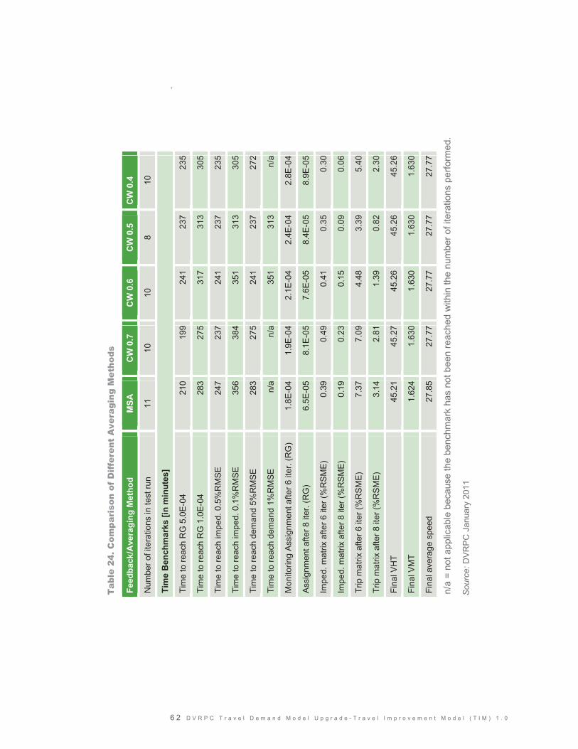
�
$ 2 � � � � � � � � � � � � � � � � � � � � � � � � � � � � � � � � � � � � � � � � � � � � � � � � � � � � � � � � � � � � � � � � � ! � � � � � � � � � �
!�
� � � �
Fe
edba
ck/A
vera
ging
Met
hod
MSA
C
W 0
.7
CW
0.6
C
W 0
.5
CW
0.4
Num
ber o
f ite
ratio
ns in
test
run
11
10
10
8 10
Tim
e B
ench
mar
ks [i
n m
inut
es]
Tim
e to
reac
h R
G 5
.0E
-04
210
199
241
237
235
Tim
e to
reac
h R
G 1
.0E
-04
283
275
317
313
305
Tim
e to
reac
h im
ped.
0.5
%R
MS
E
247
237
241
237
235
Tim
e to
reac
h im
ped.
0.1
%R
MS
E
356
384
351
313
305
Tim
e to
reac
h de
man
d 5%
RM
SE
28
327
524
123
727
2
Tim
e to
reac
h de
man
d 1%
RM
SE
n/
an/
a35
131
3n/
a
Mon
itorin
g A
ssig
nmen
t afte
r 6 it
er. (
RG
) 1.
8E-0
41.
9E-0
42.
1E-0
42.
4E-0
42.
8E-0
4
Ass
ignm
ent a
fter 8
iter
. (R
G)
6.5E
-05
8.1E
-05
7.6E
-05
8.4E
-05
8.9E
-05
Impe
d. m
atrix
afte
r 6 it
er (%
RS
ME
) 0.
390.
490.
410.
350.
30
Impe
d. m
atrix
afte
r 8 it
er (%
RS
ME
) 0.
190.
230.
150.
090.
06
Trip
mat
rix a
fter 6
iter
(%R
SM
E)
7.37
7.09
4.48
3.39
5.40
Trip
mat
rix a
fter 8
iter
(%R
SM
E)
3.14
2.81
1.39
0.82
2.30
Fina
l VH
T 45
.21
45.2
745
.26
45.2
645
.26
Fina
l VM
T 1.
624
1.63
01.
630
1.63
01.
630
Fina
l ave
rage
spe
ed
27.8
527
.77
27.7
727
.77
27.7
7
Tab
le 2
4. C
ompa
riso
n of
Dif
fere
nt A
vera
ging
Met
hods
n/a
= no
t app
licab
le b
ecau
se th
e be
nchm
ark
has
not b
een
reac
hed
with
in th
e nu
mbe
r of i
tera
tions
per
form
ed.
Sou
rce:
DV
RP
C �
����
���
��
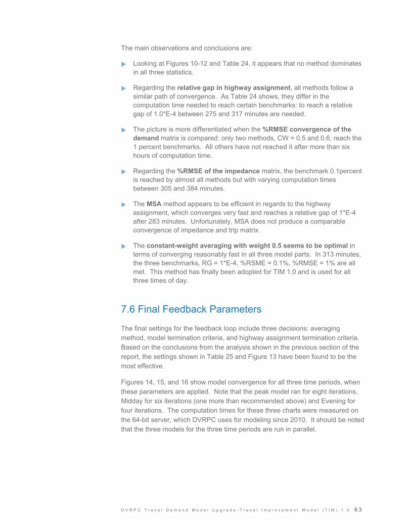
D V R P C T r a v e l D e m a n d M o d e l U p g r a d e - T r a v e l I m p r o v e m e n t M o d e l ( T I M ) 1 . 0 6 3
The main observations and conclusions are:
� Looking at Figures 10-12 and Table 24, it appears that no method dominates in all three statistics.
� Regarding the relative gap in highway assignment, all methods follow a similar path of convergence. As Table 24 shows, they differ in the computation time needed to reach certain benchmarks: to reach a relative gap of 1.0*E-4 between 275 and 317 minutes are needed.
� The picture is more differentiated when the %RMSE convergence of the demand matrix is compared: only two methods, CW = 0.5 and 0.6, reach the 1 percent benchmarks. All others have not reached it after more than six hours of computation time.
� Regarding the %RMSE of the impedance matrix, the benchmark 0.1percent is reached by almost all methods but with varying computation times between 305 and 384 minutes.
� The MSA method appears to be efficient in regards to the highway assignment, which converges very fast and reaches a relative gap of 1*E-4 after 283 minutes. Unfortunately, MSA does not produce a comparable convergence of impedance and trip matrix.
� The constant-weight averaging with weight 0.5 seems to be optimal in terms of converging reasonably fast in all three model parts. In 313 minutes, the three benchmarks, RG = 1*E-4, %RSME = 0.1%, %RMSE = 1% are all met. This method has finally been adopted for TIM 1.0 and is used for all three times of day.
7.6 Final Feedback Parameters
The final settings for the feedback loop include three decisions: averaging method, model termination criteria, and highway assignment termination criteria. Based on the conclusions from the analysis shown in the previous section of the report, the settings shown in Table 25 and Figure 13 have been found to be the most effective.
Figures 14, 15, and 16 show model convergence for all three time periods, when these parameters are applied. Note that the peak model ran for eight iterations, Midday for six iterations (one more than recommended above) and Evening for four iterations. The computation times for these three charts were measured on the 64-bit server, which DVRPC uses for modeling since 2010. It should be noted that the three models for the three time periods are run in parallel.

6 4 D V R P C T r a v e l D e m a n d M o d e l U p g r a d e - T r a v e l I m p r o v e m e n t M o d e l ( T I M ) 1 . 0
Table 25. Effective Feedback Parameters
Parameter Most effective setting
Averaging method Constant weight of 0.5 (50%)
max. iterations = 4 Assignment termination
Relative Gap = 1.0*E-4
Relative Gap = 1.0*E-4
%RMSE impedance matrix = 0.1
%RMSE trip matrix = 1.0
Max. iterations, Peak = 8
Max. iterations, Midday = 6
Feedback loop termination
Max. iterations, Evening = 4
Source: DVRPC January 2011
Figure 13. Recommended Settings for Model Run Termination
Source: DVRPC January 2011
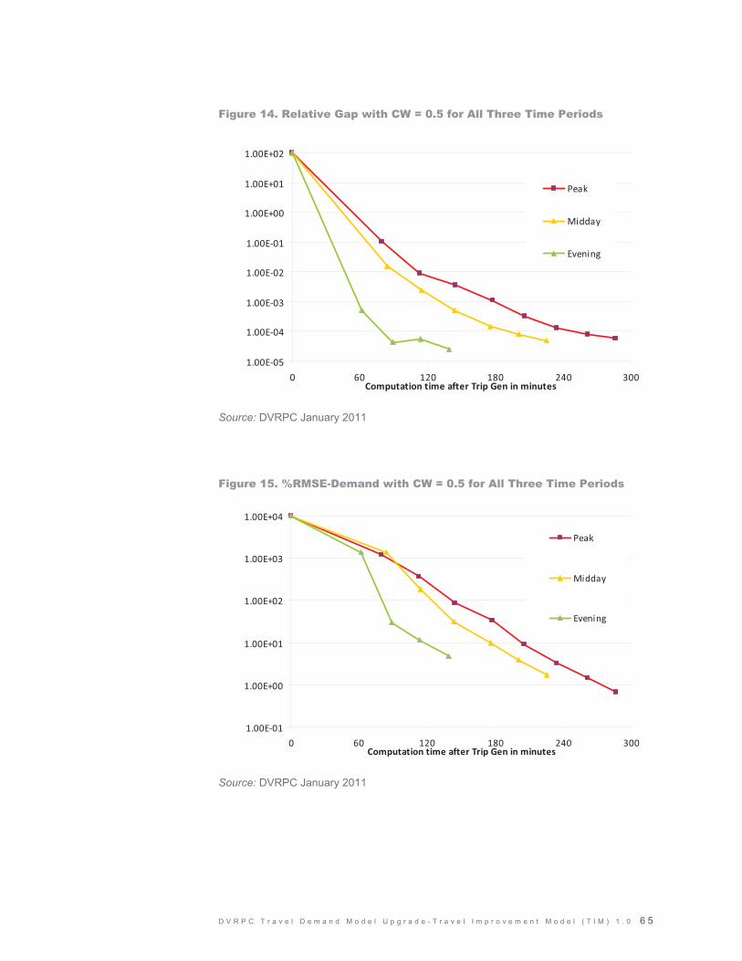
D V R P C T r a v e l D e m a n d M o d e l U p g r a d e - T r a v e l I m p r o v e m e n t M o d e l ( T I M ) 1 . 0 6 5
Figure 14. Relative Gap with CW = 0.5 for All Three Time Periods
1.00E�05
1.00E�04
1.00E�03
1.00E�02
1.00E�01
1.00E+00
1.00E+01
1.00E+02
0 60 120 180 240 300Computation�time�after�Trip�Gen�in�minutes
Peak
Midday
Evening
Source: DVRPC January 2011
Figure 15. %RMSE-Demand with CW = 0.5 for All Three Time Periods
1.00E�01
1.00E+00
1.00E+01
1.00E+02
1.00E+03
1.00E+04
0 60 120 180 240 300Computation�time�after�Trip�Gen�in�minutes
Peak
Midday
Evening
Source: DVRPC January 2011
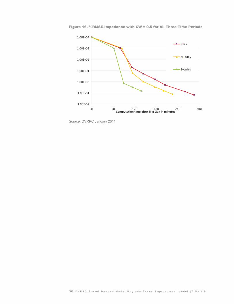
6 6 D V R P C T r a v e l D e m a n d M o d e l U p g r a d e - T r a v e l I m p r o v e m e n t M o d e l ( T I M ) 1 . 0
Figure 16. %RMSE-Impedance with CW = 0.5 for All Three Time Periods
1.00E�02
1.00E�01
1.00E+00
1.00E+01
1.00E+02
1.00E+03
1.00E+04
0 60 120 180 240 300Computation�time�after�Trip�Gen�in�minutes
Peak
Midday
Evening
Source: DVRPC January 2011
D V R P C T r a v e l D e m a n d M o d e l U p g r a d e - T r a v e l I m p r o v e m e n t M o d e l ( T I M ) 1 . 0 6 7
C H A P T E R 8
Model Validation
Since the objective of this task was to convert the already validated DVRPC TRANPLAN model to the VISUM software, the validation effort consisted mainly of ensuring that, to the extent possible, the validation results were at least as good as those for the TRANPLAN model. The checks performed included comparisons of the VISUM results to the corresponding TRANPLAN results and, where data were available, comparisons of the VISUM results to the same observed data used in the validation of the TRANPLAN model. This section presents the results of these validation checks.
There are no validation results for trip generation, including trips by time of day, since as discussed previously, the VISUM results for the internal person and vehicle trips matched the TRANPLAN results. For the external-internal trips, the results did differ, as discussed in Sections 3.2 and 3.4, but there was no observed data set available for comparison.
8.1 Trip Distribution Validation
Two main checks of trip distribution results were performed:
� Comparison of average trip lengths and trip length frequency distributions from the VISUM model to those of the TRANPLAN model, as well as to observed data from the DVRPC 2000 household travel survey (for average trip lengths)
� Comparison of county-to-county trip patterns from the VISUM model to those from the TRANPLAN model
These comparisons were performed separately for the three time periods in the model.
Table 26 compares the average trip lengths by purpose and time period. Table 27 compares the average daily trip lengths between the two models and also compares the model results to observed average trip lengths from the survey data.
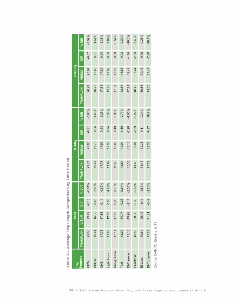
�
$ % � � � � � � � � � � � � � � � � � � � � � � � � � � � � � � � � � � � � � � � � � � � � � � � � � � � � � � � � � � � � � � � � � ! � �
��������������������������� �
Peak
M
idda
y Ev
enin
g
Trip
Pu
rpos
e TR
AN
PLA
N
VISU
M
Diff
%
Diff
TR
AN
PLA
N
VISU
M
Diff
%
Diff
TR
AN
PLA
N
VISU
M
Diff
%
Diff
HB
W
29.6
0 29
.42
-0.1
8-0
.61%
29.7
128
.80
-0.9
1 -3
.06%
28.9
128
.04
-0.8
7-3
.02%
HB
NW
16
.44
16.9
2 0.
482.
89%
16.4
716
.73
0.26
1.
59%
16.2
316
.50
0.27
1.67
%
NH
B
17.7
5 17
.86
0.11
0.62
%17
.76
17.9
90.
23
1.27
%17
.65
17.8
90.
241.
35%
Ligh
t Tru
ck
11.6
8 12
.18
0.50
4.29
%11
.62
12.3
60.
74
6.38
%12
.23
12.5
80.
352.
87%
Hea
vy T
ruck
17
.11
17.1
5 0.
030.
20%
16.6
017
.09
0.49
2.
96%
17.3
117
.22
-0.0
9-0
.54%
Taxi
13
.99
14.0
7 0.
080.
54%
13.9
414
.04
0.10
0.
71%
13.8
513
.88
0.03
0.22
%
EI-F
reew
ay
45.1
3 43
.99
-1.1
4-2
.53%
45.3
543
.15
-2.2
0 -4
.85%
47.2
142
.47
-4.7
4-1
0.0%
EI-A
rteria
l 40
.89
38.6
0 -2
.30
-5.6
2%41
.60
39.0
1-2
.59
-6.2
2%40
.43
37.4
4-2
.99
-7.4
0%
EI-L
ocal
30
.84
29.4
2 -1
.41
-4.5
9%31
.47
31.3
6-0
.11
-0.3
4%30
.56
30.4
8-0
.08
-0.2
6%
EI-T
urnp
ike
77.7
3 71
.31
-6.4
2-8
.26%
77.7
269
.35
-8.3
7 10
.8%
75.0
067
.41
-7.6
0-1
0.1%
Tab
le 2
6. A
vera
ge T
rip
Leng
th C
ompa
riso
n by
Tim
e P
erio
d
Sou
rce:
DV
RP
C �
����
���
��

�
� � � � � � � � � � � � � � � � � � � � � � � � � � � � � � � � � � � � � � � � � � � � � � � � � � � � � � � � � � � � � � � � ! � $ & ��
�
� � � ����� �������������������������� ����� ���� � �
VISU
M
TRA
NPL
AN
Trip
Typ
e
Obs
erve
d Tr
ip
Leng
th S
urve
yed
(Min
utes
)
Trip
Len
gth
Sim
ulat
ed
(Min
utes
) Pe
rcen
t D
iffer
ence
Trip
Len
gth
Sim
ulat
ed
(Min
utes
) Pe
rcen
t D
iffer
ence
Inte
rnal
-Inte
rnal
Trip
Pro
duct
ions
Hom
e-B
ased
Wor
k 26
.128
.9
10.9
%29
.412
.8%
Hom
e-B
ased
Non
-Wor
k 16
.716
.7
0.3%
16.4
-1.8
%
Non
-Hom
e-B
ased
17
.817
.9
0.8%
17.7
-0.3
%
Ext
erna
l-Trip
Attr
actio
ns
Turn
pike
s 70
.169
.2
-1.2
%76
.79.
4%
Free
way
s 41
.643
.2
3.9%
46.0
10.6
%
Arte
rials
35
.038
.4
9.6%
41.0
17.1
%
Loca
l Stre
ets
27.9
30.3
8.
7%30
.910
.9%
Truc
k Tr
ip O
rigin
s
Ligh
t Tru
ck
17.4
12.4
-2
9.0%
11.8
-32.
1%
Hea
vy T
ruck
23
.617
.1
-27.
4%17
.0-2
8.1%
Taxi
Trip
Orig
ins
15.2
14.0
-7
.9%
13.9
-8.3
%
Tab
le 2
7. A
vera
ge D
aily
Tri
p Le
ngth
Com
pari
son
Sou
rce:
DV
RP
C �
����
���
��
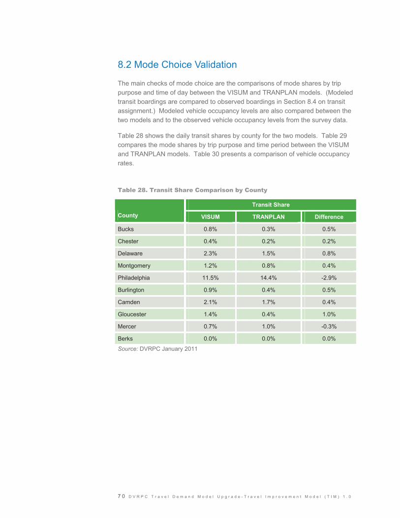
7 0 D V R P C T r a v e l D e m a n d M o d e l U p g r a d e - T r a v e l I m p r o v e m e n t M o d e l ( T I M ) 1 . 0
8.2 Mode Choice Validation
The main checks of mode choice are the comparisons of mode shares by trip purpose and time of day between the VISUM and TRANPLAN models. (Modeled transit boardings are compared to observed boardings in Section 8.4 on transit assignment.) Modeled vehicle occupancy levels are also compared between the two models and to the observed vehicle occupancy levels from the survey data.
Table 28 shows the daily transit shares by county for the two models. Table 29 compares the mode shares by trip purpose and time period between the VISUM and TRANPLAN models. Table 30 presents a comparison of vehicle occupancy rates.
Table 28. Transit Share Comparison by County
Transit Share
County VISUM TRANPLAN Difference
Bucks 0.8% 0.3% 0.5%
Chester 0.4% 0.2% 0.2%
Delaware 2.3% 1.5% 0.8%
Montgomery 1.2% 0.8% 0.4%
Philadelphia 11.5% 14.4% -2.9%
Burlington 0.9% 0.4% 0.5%
Camden 2.1% 1.7% 0.4%
Gloucester 1.4% 0.4% 1.0%
Mercer 0.7% 1.0% -0.3%
Berks 0.0% 0.0% 0.0%
Source: DVRPC January 2011
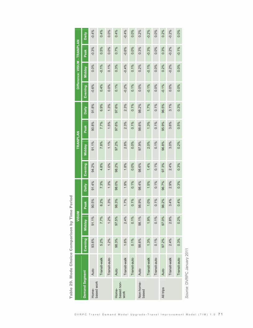
�
� � � � � � � � � � � � � � � � � � � � � � � � � � � � � � � � � � � � � � � � � � � � � � � � � � � � � � � � � � � � � � � � ! � " � �
�
VISU
M
TRA
NPL
AN
D
iffer
ence
: VIS
UM
- TR
AN
PLA
N
Dem
and
Segm
ent
Even
ing
Mid
day
Peak
D
aily
Ev
enin
g M
idda
y Pe
ak
Dai
ly
Even
ing
Mid
day
Peak
D
aily
Aut
o 93
.6%
91
.1%
90.5
%91
.4%
94.2
%91
.1%
90.8
%91
.8%
-0.6
%0.
0%-0
.3%
-0.4
%
Tran
sit-w
alk
5.2%
7.
7%8.
2%7.
3%4.
8%7.
8%7.
7%6.
9%0.
4%-0
.1%
0.5%
0.4%
Hom
e-
base
d w
ork
Tran
sit-a
uto
1.2%
1.
2%1.
3%1.
3%1.
0%1.
1%1.
5%1.
3%0.
0%0.
1%0.
0%0.
0%
Aut
o 98
.3%
97
.5%
98.3
%98
.0%
98.2
%97
.2%
97.6
%97
.6%
0.1%
0.3%
0.7%
0.4%
Tran
sit-w
alk
1.6%
2.
4%1.
7%1.
9%1.
8%2.
8%2.
3%2.
3%-0
.2%
-0.4
%-0
.6%
-0.4
%
Hom
e-ba
sed
non-
wor
k
Tran
sit-a
uto
0.1%
0.
1%0.
1%0.
1%0.
0%0.
0%0.
1%0.
1%0.
1%0.
1%0.
0%0.
0%
Aut
o 98
.6%
98
.1%
98.9
%98
.4%
98.6
%97
.9%
98.6
%98
.2%
0.0%
0.2%
0.3%
0.2%
Tran
sit-w
alk
1.3%
1.
9%1.
0%1.
5%1.
4%2.
0%1.
3%1.
7%-0
.1%
-0.1
%-0
.3%
-0.2
%
Non
-hom
e-
base
d
Tran
sit-a
uto
0.1%
0.
1%0.
1%0.
1%0.
1%0.
1%0.
1%0.
1%0.
0%0.
0%0.
0%0.
0%
Aut
o 97
.2%
97
.0%
96.2
%96
.7%
97.3
%96
.8%
95.9
%96
.5%
-0.1
%0.
2%0.
3%0.
2%
Tran
sit-w
alk
2.4%
2.
8%3.
4%2.
9%2.
4%3.
0%3.
6%3.
1%0.
0%-0
.2%
-0.2
%-0
.2%
All
trips
Tran
sit-a
uto
0.3%
0.
2%0.
4%0.
3%0.
3%0.
2%0.
5%0.
3%0.
0%0.
0%-0
.1%
0.0%
Tab
le 2
9. M
ode
Cho
ice
Com
pari
son
by T
ime
Per
iod
Sou
rce:
DV
RP
C �
����
���
��
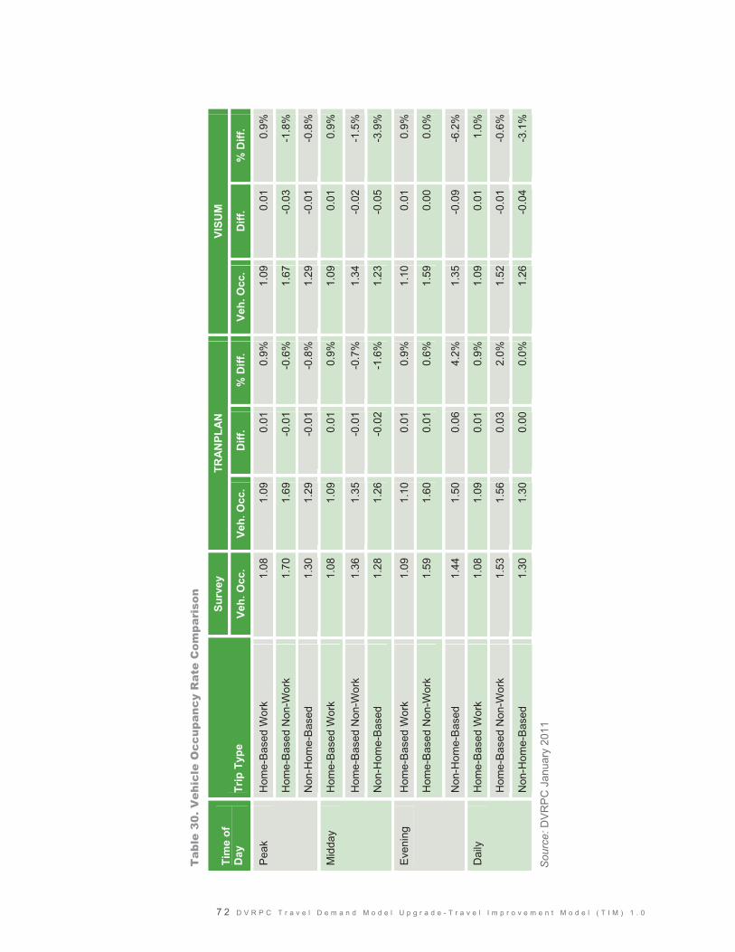
Surv
ey
TRA
NPL
AN
VI
SUM
Ti
me
of
Day
Tr
ip T
ype
Veh.
Occ
. Ve
h. O
cc.
Diff
. %
Diff
. Ve
h. O
cc.
Diff
. %
Diff
.
Hom
e-B
ased
Wor
k 1.
081.
090.
010.
9%1.
090.
010.
9%
Hom
e-B
ased
Non
-Wor
k 1.
701.
69-0
.01
-0.6
%1.
67-0
.03
-1.8
%
Pea
k
Non
-Hom
e-B
ased
1.
301.
29-0
.01
-0.8
%1.
29-0
.01
-0.8
%
Hom
e-B
ased
Wor
k 1.
081.
090.
010.
9%1.
090.
010.
9%
Hom
e-B
ased
Non
-Wor
k 1.
361.
35-0
.01
-0.7
%1.
34-0
.02
-1.5
%
Mid
day
Non
-Hom
e-B
ased
1.
281.
26-0
.02
-1.6
%1.
23-0
.05
-3.9
%
Hom
e-B
ased
Wor
k 1.
091.
100.
010.
9%1.
100.
010.
9%
Hom
e-B
ased
Non
-Wor
k 1.
591.
600.
010.
6%1.
590.
000.
0%
Even
ing
Non
-Hom
e-B
ased
1.
441.
500.
064.
2%1.
35-0
.09
-6.2
%
Hom
e-B
ased
Wor
k 1.
081.
090.
010.
9%1.
090.
011.
0%
Hom
e-B
ased
Non
-Wor
k 1.
531.
560.
032.
0%1.
52-0
.01
-0.6
%
Dai
ly
Non
-Hom
e-B
ased
1.
301.
300.
000.
0%1.
26-0
.04
-3.1
%
Tab
le 3
0. V
ehic
le O
ccup
ancy
Rat
e C
ompa
riso
n
Sou
rce:
DV
RP
C �
����
���
��
�
" � � � � � � � � � � � � � � � � � � � � � � � � � � � � � � � � � � � � � � � � � � � � � � � � � � � � � � � � � � � � � � � � � ! �
�

D V R P C T r a v e l D e m a n d M o d e l U p g r a d e - T r a v e l I m p r o v e m e n t M o d e l ( T I M ) 1 . 0 7 3
8.3 Highway Assignment Validation
Three main checks of highway assignment results were performed:
� Vehicle miles of Travel (VMT) was also compared for all highway network links between the two models and compared to VMT estimates from the Highway Performance Monitoring System (HPMS). This requires adjustments to expand the modeled VMT to VMT for all roadways; these adjustments, by county, were previously computed by DVRPC for the TRANPLAN model validation.
� Computation of percentage root mean square error between modeled and observed volumes for links with traffic counts
� Comparison of screenline volumes between the two models and observed volumes from traffic counts
Table 31 displays the VMT comparison by county for all links to the HPMS estimate. The percentage root mean square estimates between modeled volumes and counts are shown in Table 32. Table 33 presents the screenline summaries.
Table 31. VMT Comparison on All Links by County
VISUM TRANPLAN
County
HPMS VMT VMT % Diff VMT % Diff
Burlington 13,365,500 12,531,776 -6.2% 12,825,500 -4.0%
Camden 10,855,200 11,266,906 3.8% 10,661,700 -1.8%
Gloucester 7,430,700 7,853,133 5.7% 7,716,700 3.8%
Bucks 13,696,100 12,181,361 -11.1% 13,221,900 -3.5%
Mercer 9,488,200 9,918,667 4.5% 9,590,200 1.1%
Chester 11,832,000 13,024,557 10.1% 13,865,500 17.2%
Delaware 10,180,600 10,191,914 0.1% 10,061,700 -1.2%
Montgomery 19,109,500 19,024,104 -0.4% 18,915,300 -1.0%
Philadelphia 16,316,400 16,716,956 2.5% 15,538,400 -4.8%
Total 112,274,200 112,709,373 0.4% 112,396,900 0.1%
Source: DVRPC January 2011
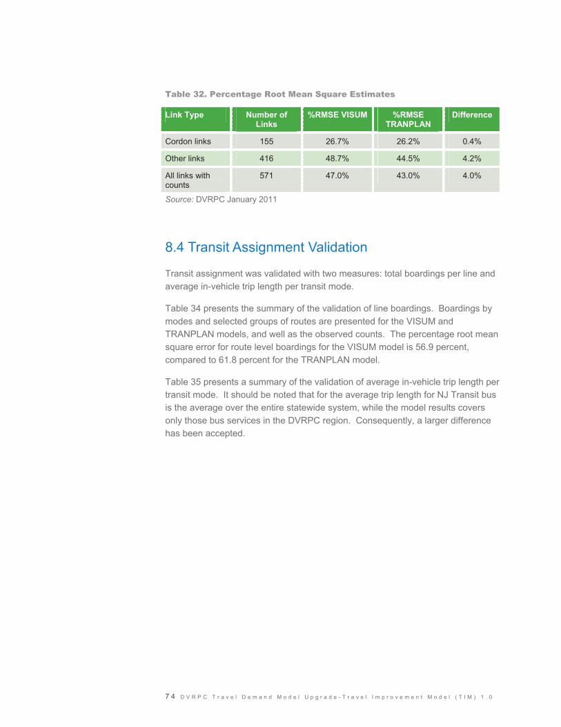
7 4 D V R P C T r a v e l D e m a n d M o d e l U p g r a d e - T r a v e l I m p r o v e m e n t M o d e l ( T I M ) 1 . 0
Table 32. Percentage Root Mean Square Estimates
Link Type Number of Links
%RMSE VISUM %RMSE TRANPLAN
Difference
Cordon links 155 26.7% 26.2% 0.4%
Other links 416 48.7% 44.5% 4.2%
All links with counts
571 47.0% 43.0% 4.0%
Source: DVRPC January 2011
8.4 Transit Assignment Validation
Transit assignment was validated with two measures: total boardings per line and average in-vehicle trip length per transit mode.
Table 34 presents the summary of the validation of line boardings. Boardings by modes and selected groups of routes are presented for the VISUM and TRANPLAN models, and well as the observed counts. The percentage root mean square error for route level boardings for the VISUM model is 56.9 percent, compared to 61.8 percent for the TRANPLAN model.
Table 35 presents a summary of the validation of average in-vehicle trip length per transit mode. It should be noted that for the average trip length for NJ Transit bus is the average over the entire statewide system, while the model results covers only those bus services in the DVRPC region. Consequently, a larger difference has been accepted.

VIS
UM
T
RA
NP
LA
N
Co
rdo
n/ S
cree
nlin
e
Co
un
t M
od
el
Dif
f %
M
od
el
Dif
f %
Buc
ks C
ount
y In
ner
Cor
don
296,
243
266,
774
-29,
469
-10%
267,
589
-28,
654
-10%
Mon
tgom
ery
Cou
nty
Inn
er C
ord
on
555,
991
504,
535
-51,
456
-9%
509,
863
-46,
128
-8%
Che
ster
Cou
nty
Inn
er C
ord
on
265,
506
234,
927
-30,
579
-12%
257,
106
-8,4
00-3
%
Del
aw
are
Cou
nty
Inn
er C
ord
on
251,
158
266,
720
15,5
62
6%27
7,7
9526
,63
711
%
Mer
cer
Co
unty
Inne
r C
ord
on
459,
013
456,
897
-2,1
16
0%42
5,8
73-3
3,14
0-7
%
Bur
lingt
on C
ount
y In
ner
Cor
don
38
5,2
2032
2,4
91-6
2,72
9 -1
6%34
7,5
39-3
7,68
1-1
0%
Cam
den
Co
unty
Inn
er C
ord
on
169,
734
158,
463
-11,
271
-7%
155,
133
-14,
601
-9%
Glo
uces
ter
Co
unty
Inne
r C
ordo
n 26
8,0
4425
8,3
93-9
,651
-4
%25
4,0
34-1
4,01
0-5
%
Su
bto
tal I
nn
er C
ord
on
2,
650,
909
2,46
9,2
00-1
81,7
09
-7%
2,49
4,9
32-1
55,9
77-6
%
Del
aw
are
Riv
er
Scr
eenl
ine
611,
134
540,
631
-70,
503
-12%
602,
531
-8,6
03-1
%
Sch
uyl
kill
Riv
er S
cree
nlin
e 1,
470,
424
1,52
0,8
9350
,46
9 3%
1,44
3,2
76-2
7,14
8-2
%
Buc
ks-M
ontg
om
ery
Cou
nty
Scr
een
line
264,
182
255,
355
-8,8
27
-3%
269,
586
5,40
42%
Cen
ter
City
Co
rdon
1,
090,
805
1,07
1,5
76-1
9,22
9 -2
%99
5,5
89-9
5,21
6-9
%
Nor
th P
hila
del
phia
Scr
eenl
ine
523,
359
540,
434
17,0
75
3%49
4,9
27-2
8,43
2-5
%
Cro
ssw
icks
Cre
ek S
cree
nlin
e 25
4,6
7225
2,3
19-2
,353
-1
%25
3,4
48-1
,224
0%
Pen
nsau
ken
Cre
ek
576,
615
602,
983
26,3
68
5%56
9,7
14-6
,901
-1%
Su
bto
tal O
ther
Scr
een
lines
4,
791,
191
4,78
4,1
91-7
,000
0
%4,
629,
071
-162
,120
-3%
9 C
ou
nty
Co
rdo
n
1,68
9,7
671,
699,
832
10,0
65
1%
1,67
2,8
04-1
6,96
3-1
%
Gra
nd
To
tal
9,13
1,8
678,
953,
223
-178
,644
-2
%8,
796,
807
-335
,060
-4%
Tab
le 3
3. S
cree
nlin
e S
umm
ary
Sou
rce:
DV
RP
C J
anua
ry 2
011
D V R P C T r a v e l D e m a n d M o d e l U p g r a d e - T r a v e l I m p r o v e m e n t M o d e l ( T I M ) 1 . 0 7 5

Mo
de
Bo
ard
ing
s C
ou
nt
Bo
ard
ing
s V
ISU
M
Dif
f. V
ISU
M
% D
iff.
VIS
UM
B
oar
din
gs
TR
AN
PL
AN
D
iff.
TR
AN
PL
AN
%
Dif
f.
TR
AN
PL
AN
Bu
s P
A
52
5,31
7
43
1,77
0
-93,
547
-1
8%
5
37,
854
1
2,5
37
2%
Bu
s N
J 5
6,5
92
81
,787
2
5,1
95
45
%
63
,543
6
,95
1
12
%
Exp
ress
bu
s P
A
55
0
90
-4
60
-84
%
96
-4
54
-83
%
Exp
ress
bu
s N
J 5
,05
2
5,0
78
2
6
1%
1,5
87
-3
,465
-6
9%
Su
bw
ay
LR
T
62
,595
8
9,0
80
26
,485
4
2%
1
16,
845
4
4,2
50
87
%
Su
bw
ay-
El
30
6,14
8
31
3,88
7
7,7
39
3%
3
07,
327
1
,17
9
0%
SE
PT
A R
eg
iona
l Ra
il 1
01,
203
1
09,
945
8
,74
2
9%
10
2,22
3
1,0
20
1%
PA
TC
O
33
,783
2
7,3
82
-6,4
01
-19
%
37
,058
3
,27
5
10
%
NJ
Re
gio
nal R
ail
10
,552
3
9,4
83
28
,931
2
74
%
13
,103
2
,55
1
24
%
To
tal c
ou
nte
d m
od
es
1
,10
1,7
91
1,0
98
,502
-3
,289
0
%
1,1
79
,636
7
7,6
76
7%
Sel
ecte
d L
ines
Ma
rke
t-F
rank
ford
1
80,
896
2
03,
786
2
2,8
90
13
%
19
6,15
4
15
,258
8%
Bro
ad
Str
eet
11
6,45
1
10
4,43
3
-12,
018
-1
0%
1
04,
804
-1
1,64
7
-10
%
RT
10
0
8,8
01
5
,66
8
-3,1
33
-36
%
6,3
69
-2
,432
-2
8%
All
Hea
vy R
ail
30
6,14
8
31
3,88
7
7,7
39
3%
3
07,
327
1
,17
9
0%
R1
4
,01
7
5,1
36
1
,11
9
28
%
4,6
44
6
27
1
6%
R2
1
3,8
42
14
,310
4
68
3%
1
5,4
34
1,5
92
1
2%
R3
1
8,2
10
18
,521
3
11
2%
1
6,6
94
-1,5
16
-8%
Sel
ecte
d L
ines
R5
3
3,4
62
24
,285
-9
,177
-2
7%
2
2,0
78
-11,
384
-3
4%
R6
7
,96
0
8,4
54
4
94
6%
1
0,0
28
2,0
68
2
6%
R7
1
3,8
50
27
,399
1
3,5
49
98
%
20
,803
6
,95
3
50
%
R8
9
,86
2
11
,840
1
,97
8
20
%
12
,542
2
,71
6
27
%
All
SE
PT
A R
eg
iona
l Ra
il 1
01,
203
1
09,
945
8
,74
2
9%
10
2,22
3
1,0
20
1%
Sou
rce:
DV
RP
C O
ctob
er 2
010
Tab
le 3
4. T
rans
it A
ssig
nmen
t V
alid
atio
n S
umm
ary
7 6 D V R P C T r a v e l D e m a n d M o d e l U p g r a d e - T r a v e l I m p r o v e m e n t M o d e l ( T I M ) 1 . 0
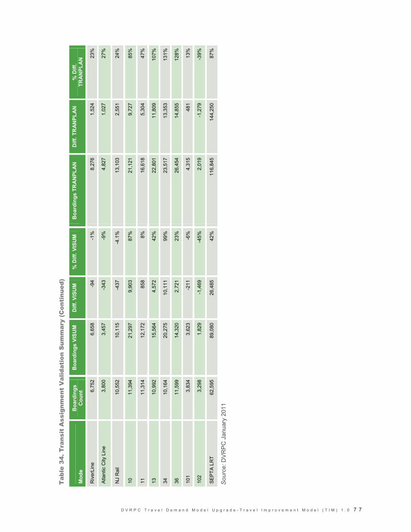
Mo
de
Bo
ard
ing
s C
ou
nt
Bo
ard
ing
s V
ISU
M
Dif
f. V
ISU
M
% D
iff.
VIS
UM
B
oar
din
gs
TR
AN
PL
AN
D
iff.
TR
AN
PL
AN
%
Dif
f.
TR
AN
PL
AN
Riv
erL
ine
6
,75
2
6,6
58
-9
4
-1%
8
,27
6
1,5
24
2
3%
Atla
ntic
City
Lin
e
3,8
00
3
,45
7
-343
-9
%
4,8
27
1
,02
7
27
%
NJ
Ra
il 1
0,5
52
10
,115
-4
37
-4.1
%
13
,103
2
,55
1
24
%
10
1
1,3
94
21
,297
9
,90
3
87
%
21
,121
9
,72
7
85
%
11
1
1,3
14
12
,172
8
58
8%
1
6,6
18
5,3
04
4
7%
13
1
0,9
92
15
,564
4
,57
2
42
%
22
,801
1
1,8
09
10
7%
34
1
0,1
64
20
,275
1
0,1
11
99
%
23
,517
1
3,3
53
13
1%
36
1
1,5
99
14
,320
2
,72
1
23
%
26
,454
1
4,8
55
12
8%
10
1
3,8
34
3
,62
3
-211
-6
%
4,3
15
4
81
1
3%
10
2
3,2
98
1
,82
9
-1,4
69
-45
%
2,0
19
-1
,279
-3
9%
SE
PT
A L
RT
6
2,5
95
89
,080
2
6,4
85
42
%
11
6,84
5
14
4,25
0
87
%
Sour
ce:
DV
RP
C J
anua
ry 2
011
Tab
le 3
4. T
rans
it A
ssig
nmen
t V
alid
atio
n S
umm
ary
(Con
tinu
ed)
D V R P C T r a v e l D e m a n d M o d e l U p g r a d e - T r a v e l I m p r o v e m e n t M o d e l ( T I M ) 1 . 0 7 7

7 8 D V R P C T r a v e l D e m a n d M o d e l U p g r a d e - T r a v e l I m p r o v e m e n t M o d e l ( T I M ) 1 . 0
Table 35. Average Transit in Vehicle Trip Length Validation
Transit on-Board Unlinked Trip Length
Transit Division 2005
Surveyed 2005
Model Diff % Diff.
SEPTA City Bus 2.61 2.35 -0.26 -10%
SEPTA Victory Bus 5.24 4.93 -0.31 -6%
SEPTA Frontier Bus 7.49 5.44 -2.05 -27%
SEPTA City Light Rail 2.26 2.28 0.02 1%
SEPTA 101, 102 3.24 3.27 0.03 1%
Market-Frankford Line 4.97 4.69 -0.28 -6%
Broad Street Line 3.73 3.19 -0.54 -15%
NHSL Line (100) 4.45 4.46 0.01 0%
SEPTA Regional Rail 14.07 12.08 -1.99 -14%
PATCO 8.62 7.46 -1.16 -13%
RiverLine 15.90 15.94 0.04 0%
NJ Transit Bus* 6.52 10.56 4.04 62%
*NJ Transit Bus 2005 Surveyed is results for entire state; model is results for just DVRPC region. Source: DVRPC January 2011

D V R P C T r a v e l D e m a n d M o d e l U p g r a d e - T r a v e l I m p r o v e m e n t M o d e l ( T I M ) 1 . 0 7 9
C H A P T E R 9
Model Run Organization
9.1 Computer Requirements
VISUM is available as a 32-bit or 64-bit executable. The VISUM model compatible with 32-bit technology for editing, but 64-bit computers are required for model runs. The computer used for model runs needs to meet the following minimal characteristics (July 2010):
� 64-bit Windows
� Multiple CPU cores, recommended
� 2 GB RAM per core, at least 4GB total
VISUM input and output files are fully compatible with either 32-bit or 64 bit, no matter how they had been created.
9.2 The Full Model Run with the Master Script
The master script DVRPCMasterBody.PY controls a sequential routine. The routine loads several PAR files in VISUM. Each PAR file contains a set of VISUM procedure steps that are then performed once or several times during a model run. If the computer has multiple cores or multiple CPUs, the process allows VISUM to run the models for the time periods in parallel.

8 0 D V R P C T r a v e l D e m a n d M o d e l U p g r a d e - T r a v e l I m p r o v e m e n t M o d e l ( T I M ) 1 . 0
To prepare the data for a full model run, the following steps need to be performed:
� Create a new folder, e.g., Run2005
� Copy into the new folder:
� VER file with all edits to network and zonal data
� 10 PAR files (DVTripGen.par, DVModelLoop*init/middle/end.par)
� All PY scripts needed for model run (currently 22 scripts)
� (Make sure the VISUMVDFDVRPCToll_V2.dll and VISUMVDFDVRPCToll_V2.bmp are in C:\Documents and Settings\***\Application Data\Visum\110\UserVDF-DLLs)
� Launch the masterscript:
� Open Masterscript\DVRPCMasterBody.PY with PythonWin and hit “run”
� When the GUI shown in Figure 17 appears, make the following interactive choices:
� Select a VER file as input for the model run
� Select the times of day to compute
Load VER file in VISUM Run trip generation (DVTripGen.par) Create a folder for each time period (PK, MD, EV) Clone the VER file
Consolidate and store data from all time periods in: *_results.VER
PK model: Run *PKInit.par n times: PKMiddle.par Run *PKEnd.par Store VER file with PK results
MD model: run *MDInit.par repeat: MDMiddle.par run *MDEnd.par Store VER file with MD results
EV model: run *EVInit.par n times: EVMiddle.par run *EVEnd.par Store VER file with EV results
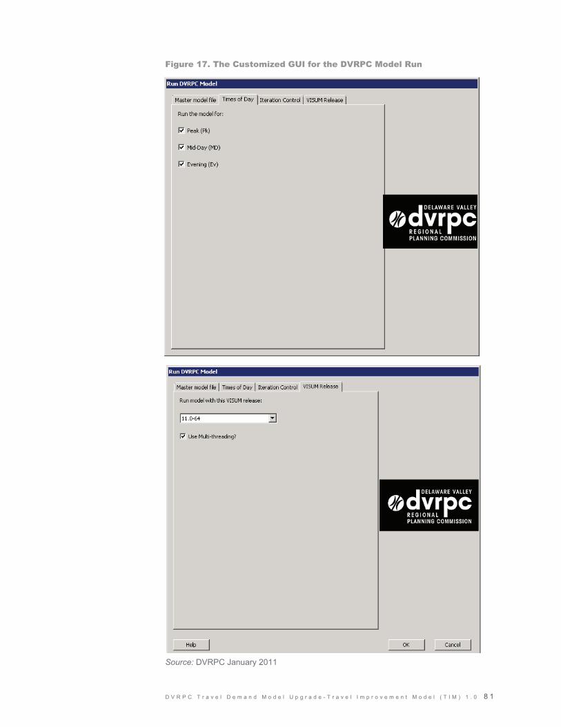
D V R P C T r a v e l D e m a n d M o d e l U p g r a d e - T r a v e l I m p r o v e m e n t M o d e l ( T I M ) 1 . 0 8 1
Figure 17. The Customized GUI for the DVRPC Model Run
�
Source: DVRPC January 2011

8 2 D V R P C T r a v e l D e m a n d M o d e l U p g r a d e - T r a v e l I m p r o v e m e n t M o d e l ( T I M ) 1 . 0
� Select convergence criteria
� Select 64 bit VISUM installation and select multi-threading if computer has multiple cores
9.3 Model Procedure in Individual Steps
This section explains all the steps of the VISUM model procedure as it is defined in the *.PAR files. As previously mentioned, there are 10 PAR files to control the entire model run:
� One PAR file for trip generation (DV_TripGen.PAR)
� Three PAR files with the initializing steps, which are executed once at the beginning of the procedure for each time period (DV_ModelLoop*INIT.PAR)
� Three PAR files with the main model steps that are repeated once in each feedback iterations (DV_ModelLoop*MIDDLE.PAR)
� Three PAR files with the final model steps that are performed one time at the very end of the procedure (DV_ModelLoop*END.PAR)
Tables 36 through 40 illustrate and comment on the content of each of the PAR files.
Table 36. Operations Procedure in Parameter File TripGen
Op. No. Name of Operation in VISUM Task Performed
How to Modify?
1 Group trip generation
2 Run script Set link cap, speed, length Python
3 Calculate skim matrix Compute hwy distance Menu
4 Run script Set distances per zone Python
5 Run script Trip generation Python
Source: DVRPC January 2011
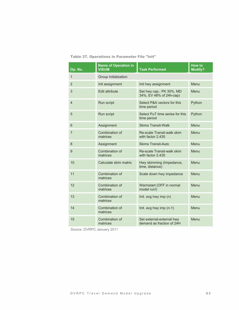
D V R P C T r a v e l D e m a n d M o d e l U p g r a d e 8 3
Table 37. Operations in Parameter File "Init"
Op. No. Name of Operation in VISUM Task Performed
How to Modify?
1 Group Initialization
2 Init assignment Init hwy assignment Menu
3 Edit attribute Set hwy cap.: PK 30%, MD 34%, EV 48% of 24h-cap)
Menu
4 Run script Select P&A vectors for this time period
Python
5 Run script Select PuT time series for this time period
Python
6 Assignment Skims Transit-Walk Menu
7 Combination of matrices
Re-scale Transit-walk skim with factor 2.435
Menu
8 Assignment Skims Transit-Auto Menu
9 Combination of matrices
Re-scale Transit-walk skim with factor 2.435
Menu
10 Calculate skim matrix Hwy skimming (Impedance, time, distance)
Menu
11 Combination of matrices
Scale down hwy impedance Menu
12 Combination of matrices
Warmstart (OFF in normal model run!)
Menu
13 Combination of matrices
Init. avg hwy imp (n) Menu
14 Combination of matrices
Init. avg hwy imp (n-1) Menu
15 Combination of matrices
Set external-external hwy demand as fraction of 24H
Menu
Source: DVRPC January 2011

8 4 D V R P C T r a v e l D e m a n d M o d e l U p g r a d e - T r a v e l I m p r o v e m e n t M o d e l ( T I M ) 1 . 0
Table 38. Operations in Parameter File "Middle"
Op. No.
Name of Operation in VISUM
Task Performed How to Modify?
1 Group Main Loop
2 Run script Average hwy impedance (core feature of feedback method)
Python
3 Trip distribution All person trips (HBW,HBNW, NHB) Menu
4 Run script TripDistributionAdjustment
Adjust trip distribution result with transit bias
Python
5 Trip distribution All vehicle trips (truck, taxi, E-I) Menu
6 Run script Captives and 0-car-HH Python
7 Mode choice HH with cars Menu
8 Mode choice HH with 0-car Menu
9 Run script Vehicle occupancy Python
10 Combination of matrices Store total highway demand from last iteration (n-1)
Menu
11 Combination of matrices Sum up highway vehicle trips for assignment
Menu
12 Combination of matrices Symmetricize hwy demand Menu
13 Combination of matrices Sum up transit-walk person trips for assignment
Menu
14 Combination of matrices Sum up transit-auto person trips for assignment
Menu
15 Combination of matrices Sum up transit-external person trips for assignment
Menu
16 Run script “GetRealZeros” Set very small numbers in trip table to 0.0
Python
17 Assignment Highway Menu
18 Calculate skim matrix Hwy skimming Menu
19 Combination of matrices Scale hwy impedance with factor 0.000406
Menu
20 Run Script “ReportConvergence”
Report convergence statistics to CSV file
Python
Source: DVRPC January 2011

D V R P C T r a v e l D e m a n d M o d e l U p g r a d e - T r a v e l I m p r o v e m e n t M o d e l ( T I M ) 1 . 0 8 5
Table 39. Operations in Parameter File "End"
Op. No. Name of Operation in VISUM Task Performed
How to Modify?
1 Group Post-Process
2 Init assignment Init transit assignment Menu
3 Assignment Transit-Auto Menu
4 Assignment Transit-Walk Menu
5 Assignment Transit-External Menu
6 Territory indicators District statistics Menu
7 Combination of matrices Sum up transit total demand
Menu
8 Run script Report matrix totals Python
9 Run script Report VMT, VHT Python
Source: DVRPC January 2011
Table 40. Differences in the PAR Files Between Time Periods
Source: DVRPC January 2011
Differences Which PAR
file Op./Step Number
Link Capacity-PrT for Hwy assignment (30% for PK, 34% for Midday and 48% for Evening)
INIT 3
P&A vectors, assigned to “Current” (a specific Python script for each time period)
INIT 4
Time series for transit demand INIT 5
Transit assignment parameters: Time interval in assignment settings
INIT 6, 8
Set the external-external demand (currently 33% for each of the three time periods)
INIT 15
Captivity in mode choice: ( a specific PY script for each time of day)
MIDDLE 6
Vehicle occupancy: (a specific PY script for each time of day)
MIDDLE 9
Transit assignment parameters: Time interval in assignment settings
END 3, 4, 5

8 6 D V R P C T r a v e l D e m a n d M o d e l U p g r a d e - T r a v e l I m p r o v e m e n t M o d e l ( T I M ) 1 . 0
All three Middle-PAR files are to a large part identical. The same applied to the three “end” and the three “init” files. There are only a few small differences between the time periods. Table 40 explains these small differences.
9.4 Results, Reports, and Protocols of the Model Run
The following listing shows where results and reports of the model run can be found:
Log, Trace, Error files
...\Run2005\log.txt
...\Run2005\PK\trace*.txt, error*.txt
...\Run2005\MD\trace*.txt, error*.txt
...\Run2005\EV\trace*.txt, error*.txt
Model Results
...\Run2005\PK\*_PK.VER - all matrices and assignment paths for peak
...\Run2005\MD\*_MD.VER - all matrices and assignment paths for midday
...\Run2005\EV\*_EV.VER - all matrices and assignment paths for evening
...\Run2005\ *_RESULTS.VER - selected 24H results of the model
Model Run Reports
...\Run2005\*.csv
...\Run2005\PK\*.csv
...\Run2005\MD\*.csv
...\Run2005\EV\*.csv
9.5 Trip Purposes and Demand Stratification
Table 41 presents the time periods, which are treated as “person groups” in VISUM. Table 42 presents the trip purposes, which are treated as “activity pairs” in VISUM.

D V R P C T r a v e l D e m a n d M o d e l U p g r a d e - T r a v e l I m p r o v e m e n t M o d e l ( T I M ) 1 . 0 8 7
Table 41. Time of Day as "Persons Groups" in VISUM
Code Name
Current Current Time of Day
Dly Daily
PK Peak Demand
MD Midday Demand
EV Evening Demand
Source: DVRPC January 2011 Note that “current” is the group that is used in trip distribution and mode choice steps. The three groups names after time of day periods (PK, MD, and EV) are only relevant for trip generation. The “daily” group is used for trip generation of non-motorized trips and to store trip tables of 24H.
In VISUM, “person groups” and “activity pairs” are combined to “demand strata”. As a result there could be a maximum of 5 times 22 = 110 demand strata in the model. The current model has 52 demand strata defined. Most of these 52 demand strata are only used for trip generation. Thirteen are used for either trip distribution and/or mode choice. Table 43 lists the 13 demand strata and the IDs of the OD matrices assigned to them for trip distribution and mode choice.
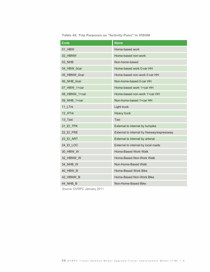
8 8 D V R P C T r a v e l D e m a n d M o d e l U p g r a d e - T r a v e l I m p r o v e m e n t M o d e l ( T I M ) 1 . 0
Table 42. Trip Purposes as "Activity Pairs" in VISUM
Code Name
01_HBW Home-based work
02_HBNW Home-based non-work
03_NHB Non-home-based
04_HBW_0car Home-based work 0-car HH
05_HBNW_0car Home-based non-work 0-car HH
06_NHB_0car Non-home-based 0-car HH
07_HBW_1+car Home-based work 1+car HH
08_HBNW_1+car Home-based non-work 1+car HH
09_NHB_1+car Non-home-based 1+car HH
11_LTrk Light truck
12_HTrk Heavy truck
13_Taxi Taxi
21_EI_TPK External to internal by turnpike
22_EI_FRE External to internal by freeway/expressway
23_EI_ART External to internal by arterial
24_EI_LOC External to internal by local roads
30_HBW_W Home-Based Work Walk
32_HBNW_W Home-Based Non-Work Walk
34_NHB_W Non-Home-Based Walk
40_HBW_B Home-Based Work Bike
42_HBNW_B Home-Based Non-Work Bike
44_NHB_B Non-Home-Based Bike
Source: DVRPC January 2011
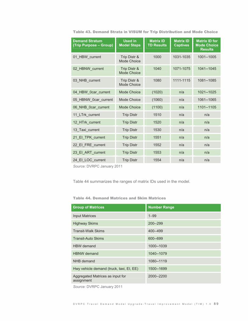
D V R P C T r a v e l D e m a n d M o d e l U p g r a d e - T r a v e l I m p r o v e m e n t M o d e l ( T I M ) 1 . 0 8 9
Table 43. Demand Strata in VISUM for Trip Distribution and Mode Choice
Demand Stratum (Trip Purpose – Group)
Used in Model Steps
Matrix ID TD Results
Matrix ID Captives
Matrix ID forMode Choice
Results
01_HBW_current Trip Distr & Mode Choice
1000 1031-1035 1001--1005
02_HBNW_current Trip Distr & Mode Choice
1040 1071-1075 1041--1045
03_NHB_current Trip Distr & Mode Choice
1080 1111-1115 1081--1085
04_HBW_0car_current Mode Choice (1020) n/a 1021--1025
05_HBNW_0car_current Mode Choice (1060) n/a 1061--1065
06_NHB_0car_current Mode Choice (1100) n/a 1101--1105
11_LTrk_current Trip Distr 1510 n/a n/a
12_HTrk_current Trip Distr 1520 n/a n/a
13_Taxi_current Trip Distr 1530 n/a n/a
21_EI_TPK_current Trip Distr 1551 n/a n/a
22_EI_FRE_current Trip Distr 1552 n/a n/a
23_EI_ART_current Trip Distr 1553 n/a n/a
24_EI_LOC_current Trip Distr 1554 n/a n/a
Source: DVRPC January 2011
Table 44 summarizes the ranges of matrix IDs used in the model.
Table 44. Demand Matrices and Skim Matrices
Group of Matrices Number Range
Input Matrices 1–99
Highway Skims 200--299
Transit-Walk Skims 400--499
Transit-Auto Skims 600--699
HBW demand 1000--1039
HBNW demand 1040--1079
NHB demand 1080--1119
Hwy vehicle demand (truck, taxi, EI, EE) 1500--1699
Aggregated Matrices as input for assignment
2000--2200
Source: DVRPC January 2011


A P P E N D I X
Fare System Documentation

D V R P C T r a v e l D e m a n d M o d e l U p g r a d e - T r a v e l I m p r o v e m e n t M o d e l ( T I M ) 1 . 0 A – 1
Fare System Documentation
Fare System
VISUM 11.0’s fare modeling system was built around European through ticketing systems, where the fare depends on the origin and destination. It was not built to handle the relatively more complicated American fare systems where transfer fares are dependant on both the mode transferred to, and transferred from. For example, the cost to transfer to the Market Frankford line at City Hall Station depends on which mode a passenger is transferring from – a transfer from the Broad Street Line is free, a transfer from a SEPTA bus is $0.75, and a transfer from the SEPTA Regional Rail system requires a full fare. VISUM 11.0 can not handle this complexity. For this reason, a few creative measures were implemented within TIM 1.0 in order to closely approximate the fare system present among the multiple modes and operators, in the Delaware Valley region. The process is similar to the fare system DVRPC used with their TRANPLAN model in the past. The next release of VISUM, 11.5, will address the complexity issues of the DVRPC region’s fare system.
The following steps describe how to maintain and update the fare structure in model:
1. Define the Transit System (Tsys) – All transit operations with distinct fare structures must be an independent Tsys. A new Tsys must be defined for any new transit service being modeled with a separate fare structure.
2. Define the fare zone boundaries – Similar to the TRANPLAN model, true matrix type zonal fare structures are not possible. Instead, average incremental fares are used. Average incremental zonal fares should be placed at links crossing zone boundaries. The fare points on the link should be equal to the fare increment in cents. See Figure A-1.
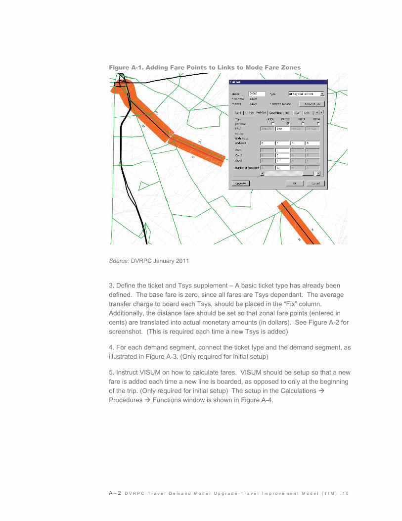
A – 2 D V R P C T r a v e l D e m a n d M o d e l U p g r a d e - T r a v e l I m p r o v e m e n t M o d e l ( T I M ) . 1 0
Figure A-1. Adding Fare Points to Links to Mode Fare Zones
Source: DVRPC January 2011
3. Define the ticket and Tsys supplement – A basic ticket type has already been defined. The base fare is zero, since all fares are Tsys dependant. The average transfer charge to board each Tsys, should be placed in the “Fix” column. Additionally, the distance fare should be set so that zonal fare points (entered in cents) are translated into actual monetary amounts (in dollars). See Figure A-2 for screenshot. (This is required each time a new Tsys is added)
4. For each demand segment, connect the ticket type and the demand segment, as illustrated in Figure A-3. (Only required for initial setup)
5. Instruct VISUM on how to calculate fares. VISUM should be setup so that a new fare is added each time a new line is boarded, as opposed to only at the beginning of the trip. (Only required for initial setup) The setup in the Calculations � Procedures � Functions window is shown in Figure A-4.

�
�
�
Figu
re A
-2. D
efin
ing
Tsy
s S
uppl
emen
ts
� � � � � � � � � � � � Sou
rce:
�� �
��
�(��
���
)���
��
Sou
rce:
�� �
��
����
����
��
��� �
�
� � � � � � � � � � � � � � � � � � � � � � � � � � � � � � � � � � � � � � � � � � � � � � � � � � � � � � � � � � � � � � � � ! � * + , �
������������
��
�

A – 4 D V R P C T r a v e l D e m a n d M o d e l U p g r a d e - T r a v e l I m p r o v e m e n t M o d e l ( T I M ) . 1 0
Figure A-3. Connecting PuT Tickets with Demand Segments
Figu
re A
-3. C
onne
ctin
g P
ut T
icke
ts w
ith
Dem
and
Seg
men
ts
Sou
rce:
DV
RP
C J
anu
ary
201
1

D V R P C T r a v e l D e m a n d M o d e l U p g r a d e - T r a v e l I m p r o v e m e n t M o d e l ( T I M ) 1 . 0 A – 5
Figure A-4. Instructing VISUM to Calculate Fare Separately for each Path Leg (transfer)
Source: DVRPC January 2011
6. The fare, setup via the Tsys supplements, charges the transfer fare at each boarding. However, we need to charge slightly more for the initial boarding. This is done using some creativity within the VISUM software. VISUM is setup to include a Tsys time attribute at the first boarding. The difference between boarding fare and transfer fare is first converted to a time element and stored as a Tsys User Defined Attribute (UDA). This should be done every time a new Tsys is created. For bookkeeping, both the extra fare in dollar amount, plus the extra fare converted to seconds and multiplied by the weight, is added as a UDA. The combined multiplier for both the conversion to time and the impedance weighting for fare in 360. The current charges are shown in Figure A-5.

A – 6 D V R P C T r a v e l D e m a n d M o d e l U p g r a d e - T r a v e l I m p r o v e m e n t M o d e l ( T I M ) . 1 0
Figure A-5. Defining Extra Boarding Charge by Tsys
Source: DVRPC January 2011
The Public Transit (PuT) impedance is then set to include this extra charge at the initial boarding. This is done via the Extended Impedance function, as illustrated in Figure A-6. (Only required for initial setup)
7. Two additional elements of cost need to be added onto the associated auto access link, when coding transit systems. The first, is the out of pocket cost to driving to a park and ride lot, and is added to the auto access link in cents. Rates of ~$0.49 are traditionally used in the DVRPC model as fare points. See illustration in Figure A-7. The second is the cost of parking, in terms of cents, and placed with a new UDA.
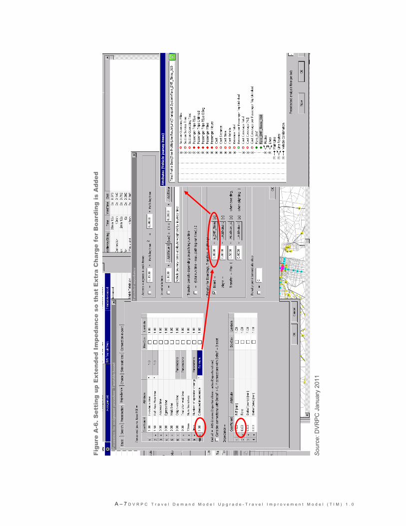
A – 7 D V R P C T r a v e l D e m a n d M o d e l U p g r a d e - T r a v e l I m p r o v e m e n t M o d e l ( T I M ) 1 . 0
Figure A-6. Setting up Extended Impedance so that Extra Charge for Boarding is added
Figu
re A
-6. S
etti
ng u
p E
xten
ded
Impe
danc
e so
tha
t E
xtra
Cha
rge
for
Boa
rdin
g is
Add
ed
Sou
rce:
DV
RP
C J
anu
ary
201
1
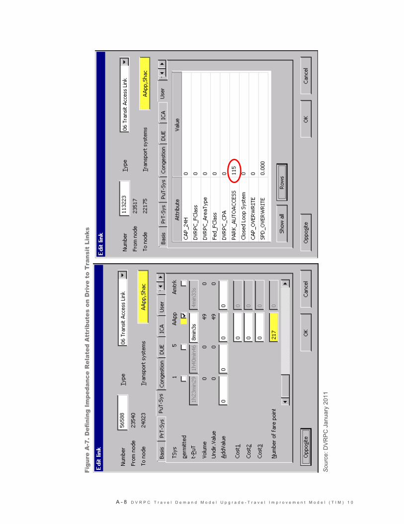
A - 8 D V R P C T r a v e l D e m a n d M o d e l U p g r a d e - T r a v e l I m p r o v e m e n t M o d e l ( T I M ) 1 0
Figure A- 7. Defining Impedance Related Attributes on Drive to Transit Links
Figu
re A
-7. D
efin
ing
Impe
danc
e R
elat
ed A
ttri
bute
s on
Dri
ve t
o T
rans
it L
inks
Sou
rce:
DV
RP
C J
anu
ary
201
1
VISUM, Python, travel demand model, TRANPLAN, Travel Forecasting Model,
FTA Compliant, Traffic Analysis Zones (TAZs) Trip Generation, Trip Distribution,
Highway Capacities and Travel and Transit Speeds, Highway Functional
Classification, Modal Split, Highway Assignment, Transit Assignment, Focused
Traffic Assignment, Transportation Improvement Model (TIM)
This report presents the results of the conversion of the Commission’s travel
demand model from TRANPLAN to the more modern VISUM software package.
This work has been undertaken by Cambridge Systematics, Inc. (CS) and PTV
America, Inc. under contract to DVRPC.
Wolfgang Scherr
Senior Transportation Engineer
(215) 238-2885
Christopher M. Puchalsky, Ph.D.
Manager, Office of Modeling and Analysis
(215) 238-2949
Delaware Valley Regional Planning Commission
190 N. Independence Mall West, 8th Floor
Philadelphia PA 19106-1520
Phone: (215) 592-1800
Fax: (215) 592-9125
Internet: www.dvrpc.org
Publication Title: DVRPC Travel Demand Model Upgrade -
Travel Improvement Model (TIM) 1.0
Publication Number: TR10006
Date Published: January 2011
Geographic Area Covered:
The Delaware Valley Region is comprised of five
counties in Pennsylvania (Bucks, Chester,
Delaware, Montgomery, and Philadelphia); and four
counties in New Jersey (Burlington, Camden,
Gloucester, and Mercer). Three municipalities in
Berks County, Pennsylvania are also included for
modeling purposes.
Key Words
Abstract
Staff Contact:
Staff Contact:

190 N Independence Mall West ACP Building, 8th Floor Philadelphia, PA 19106-1520 Phone: 215-592-1800 Fax: 215-592-9125 Website: www.dvrpc.org