SC IEN C E

13. F. Mansfeld, Corrosion 44(1988): p. 856.14. F. Mansfeld and C.H. Tsai, submitted to Corrosion.15. W. Siedlarek, W. Mader, and W. Fischer, Farbe und Lacke 90(1984): p. 824.

16. M. Ebert, Diplomarbeit Universitat Karisruhe 1986.17. G.H. Wagner, Pitture e vernici 7(1984): p. 105.18. M.W. Kendig, A.T. Allen, F. Mansfeld J. Electrochem. Soc. 131(1984): p. 935.19. F. Mansfeld, M.W. Kendig, and W.J. Lorenz, J. Electrochem. Soc. 132(1985): p.

290.20. K. Jüttner, K. Manandhar, U. Seifer-Kraus, W.J. Lorenz, and E. Schmidt, Werk-

stoffe und Korrosion 37(1986): p. 377.21. K. Jüttner, W.J. Lorenz, M.W. Kendig, and F. Mansfeld, J. Electrochem Soc.

135(1988): p. 335.22. M. Mitzlaff, H.N. Hoffmann, K. Jüttner, and W.J. Lorenz, Ber. Bunsenges. Phys.

Chem. 92(1988): p. 1234.23. W.J. Lorenz and H. Fischer, Electrochim. Acta 11(1966): p. 1597.

24. W.J. Lorenz, K. Sarropoulos, and H. Fischer, Electrochim. Acta 14(1969): p. 179.25. J. Hitzig, K. Jüttner, W.J. Lorenz, and W. Paatsch, J. Electrochem. Soc.

133(1986): p.887.26. W. Paatsch, W.J. Lorenz, and K. Jüttner, Metalloberflache 41(1987): p. 282.27. K. Jüttner and W.J. Lorenz, "Dynamic System Analysis in Corrosion Research

and Testing," in Proceedings of the 101h International Congress on Metallic Cor-rosion, vol. 1 (New Delhi, India: Oxford & IBH Publishing, 1987), p. 457.

28. K. Jüttner, W.J. Lorenz, and W. Paatsch, Corrosion Sci. 29(1989): p. 279.29. K. Jüttner and W.J. Lorenz, Materials Science Forum 44 and 45 (1989): p. 191.30. K. Jüttner and W.J. Lorenz, "Surface Inhomogeneity Characterized by EIS," in

Proceedings of the Symposium on Transient Techniques in Corrosion Scienceand Engineering, vol. 89-1 (Pennington, NJ: The Electrochemical Society Inc.,1989), p. 68.

31. J. Titz and G.H. Wagner, BASF Internal Research Report (Ludwigshafen, FRG:BASF, 1989).

Some Advantages and Pitfailsof Electrochemical Impedance Spectroscopy

D.D. Macdonald

ABSTRACT

The use of electrochemical impedance spectroscopy (EIS) in cor-rosion research is briefly reviewed with particular emphasis onthe advantages offered by this technique over other electrochemi-cal methods. These advantages include the fact that it is asteady-state technique, that it employs smalt signal analysis, andthat is capable of probing relaxations over a very wide frequencyrange (<1 mHz to >1 MHZ) using readily available istrumenta-tion. EIS also has the enormous advantage over classical tran-sient techniques in that the validity of the data is readily checkedusing the Kramers-Kronig transforms. The principal pitfall of themethod is the tendency of many workers to analyze their data interms of simple equivalent electrical circuits, and hence to ignorethe great power of EIS for deriving mechanistic and kinetic infor-mation for processes that occur at a corroding interface.

KEY WORDS: corrosion rate, electrochemical impedance spec-troscopy, reaction mechanisms.

INTRODUCTION

Electrochemical impedance spectroscopy (EIS) is now wellestablished 1-5 as a powerful technique for investigating electro-chemical and corrosion systems. The power of EIS lies in the factthat it is essentially a steady-state technique that is capable of ac-cessing relaxation phenomena whose relaxation times vary overmany orders of magnitude. The steady-state character permits theuse of signal averaging within a single experiment to gain the de-sired level of precision, and the wide frequency bandwidth (10 6 to10 -4 Hz) that is now available using transfer function analyzerspermits a wide range of interfacial processes to be investigated.These features generally surpass the equivalent performancecharacteristics for time domain experimental techniques, 4 so thatEIS has rapidly developed as one of the principal methods for in-vestigating interfacial reaction mechanisms.

Submitted for publication May 1989; in revised form, October 1989. Presented as

paper no. 30 at CORROSION/89 in New Orleans, Louisiana, April 1989.

SRI International, 333 Ravenswood Ave., Menlo Park, CA 94025.

In this paper, the foundations of EIS are briefly reviewed withparticular emphasis on corrosion science and engineering. Be-cause impedance spectroscopy is a relatively new technique, atleast in its application in corrosion science and electrochemistry,its theoretical basis has not been extensively treated in standardtexts. Accordingly, we begin this review by discussing, in very gen-eral terms, transfer-function analysis before progressing to themuch more specific task of illustrating the advantages and pitfallsof EIS as it is employed in the study of corrosion processes.

Unfortunately, there is no "easy" way of developing the skillsand expertize necessary to properly interpret impedance data. Ac-cordingly, it is essential that the reader follow the mathematicaldevelopments presented in this paper, as well as develop an ap-preciation for the electrochemistry involved in the various analyti-cal techniques. Because this paper is intended to be tutorial in na-ture and to illustrate some of the advantages and pitfalls of EIS,the essential mathematical arguments are developed in detail andin some length, rather than simply stating the problem and pre-senting the solution. While this renders the discussion somewhatverbose, it does allow the reader who is not familiar with EIS tograsp the mechanics of analyzing impedance data. Where appro-priate, the analytical methods are illustrated by reference to exper-imental studies that have been reported in the literature.

FUNDAMENTALS

The response of any linear system to a perturbation of arbi-trary form may be described by a transfer function

H(s) = V(s)/I(s) (1)

where s is the Laplace frequency, and V(s) and I(s) are the La-place transforms of the time-dependent voltage and current,respectively. 6 In terms of the steady-state sinusoidal frequencydomain, the transfer function becomes

0010-9312/90/000071 /$3.00/0

CORROSION -Vol. 46, No. 3 © 1990, National Association of Corrosion Engineers 229

SCIENCE

H(jw) = F{V(t)} / F{I(t)} = V(jw) / I(j) (2)

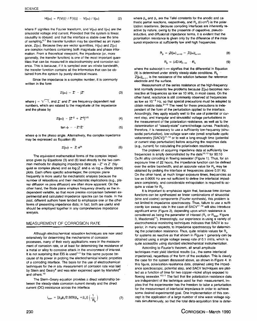
where F signifies the Fourier transform, and V(jw) and l(jw) are thesinusoidal voltage and current. Provided that the system is linear,causality is obeyed, and that the interface is stable over the timeof sampling,6 • 7 the transfer function may be identified as an inped-ance, Z(jw). Because they are vector quantities, H(jw) and Z(j )are complex numbers containing both magnitude and phase infor-mation. From a theoretical viewpoint, the impedance (or, moregenerally, the transfer function) is one of the most important quan-tities that can be measured in electrochemistry and corrosion sci-ence. This is because, if it is sampled over an infinite bandwidth,the transfer function contains all the information that can be ob-tained from the system by purely electrical means.

Since the impedance is a complex number, it is commonlywritten in the form

Z(j(0) = Z' - jZ' (3)

where j =, and Z' and Z" are frequency-dependent realnumbers, which are related to the magnitude of the impedanceand the phase by

ZGW)I = [Z,2 + Z,2] ,i2 (4)

tan 4) = -Z"/Z' (5)

where 4) is the phase angle. Alternatively, the complex inpedancemay be expressed as Equation (6)

Z(o) = I ZI e'^ (6)

The equivalent mathematical forms of the complex imped-ance given by Equations (3) and (6) lead directly to the two com-mon methods for displaying impedance data: as -Z" vs Z' (Ny-quist or complex plane) and as log IZE and 4) vs log o (Bode plane)plots. Each offers specific advantages; the complex planefrequently is more useful for mechanistic analysis because thenumber of relaxations and their mechanistic implications (e.g., pla-nar diffusion vs pore diffusion) are often more apparent. On theother hand, the Bode plane employs frequency directly as the in-dependent variable, so that more precise comparison between ex-perimental and calculated impedance spectra can be made. In thepast, different authors have tended to emphasize one or the otherforms of presenting impedance data; in fact, both are useful andshould be employed together in any comprehensive impedanceanalysis.

MEASUREMENT OF CORROS I ON RATE

Although electrochemical relaxation techniques are now usedextensively for determining the mechanisms of corrosionprocesses, many of their early applications were in the measure-ment of corrosion rate, or at least for determining the resistance ofa metal or alloy to corrosive attack in the environment of interest.It is not surprising that EIS is used 1-3 for this same purpose be-cause of its power in probing the electrochemical kinetic propetiesof a corroding interface. The basis for the use of electrochemicaltechniques for the in situ measurement of corrosion rate was laidby Stern and Geary8 and was later expanded upon by Mansfeldg

and others. 1°

The Stern-Geary equation provides a direct relationship be-tween the steady-state corrosion current density and the directcurrent (DC) resistance across the interface

1

icorr = [I3a1c/2 .303 (133 + I3c)] ( R ) (7)P

where j3a and P. are the Tafel constants for the anodic and ca-thodic partial reactions, respectively, and RP (St•cm2) is the polar-ization resistance. Because corroding interfaces are inherently re-active by nature, owing to the presence of capacitive, pseudo-inductive, and diffusional impedance terms, it is evident that thepolarization resistance is given only by the difference of the mea-sured impedance at sufficiently low and high frequencies.

RP = IZ(1-)Iw-•o - Z(jW)I,. (8)

RP = (aE1ai),. - Rs

(9)

where the subscript t-o signifies that the differential in Equation(9) is determined under strictly steady-state conditions. R. =Z(jw)Iw- is the resistance of the solution between the referenceelectrode and the surface.

Measurement of the series resistance at the high-frequencylimit normally presents few problems because Z(jo) becomes non-reactive at frequencies as low as 10 kHz, in most cases. On theother hand, reactance is still commonly observed at frequenciesas low as 10 -3 Hz, so that special precautions must be adopted toobtain reliable data. 2-10 The need for these precautions is inde-pendent of the form of the perturbation applied to the interface.Accordingly, they apply equally well to the use of potential or cur-rent step, and triangular and sinusoidal voltage perturbations inthe measurement of the polarization resistance, as well as to thedetermination of "steady-state" current/voltage curves. Practically,therefore, it is necessary to use a sufficiently low-frequency (sinu-soidal perturbation), low-voltage scan rate (small amplitude cyclicvoltammetry [SACV])"•' Z or to wait a long enough time (potentialor current step perturbation) before acquiring the response data(e.g., current) for calculating the polarization resistance.

The problem of acquiring impedance data at sufficiently lowfrequencies is amply demonstrated by the data 10 • 13 for 90:10Cu:Ni alloy corroding in flowing seawater (Figure 1). Thus, for anexposure time of 22 hours, the impedance function can be definedover the entire bandwidth, and an accurate value for R P may beobtained by probing the interface at frequencies above 0.01 Hz.On the other hand, at much longer exposure times, frequencies aslow as 0.0005 Hz are not sufficient to define the interfacial imped-ance completely, and considerable extrapolation is required to ac-quire a value for R.

It is important to emphasize again that, because time dornainfunctions can be synthesized as linear combinations of sinusoidal(sine and cosine) components (Fourier synthesis), this problem isnot limited to impedance spectroscopy. Thus, failure to use a suffi-ciently low sweep rate in the case of SACV112 will also introducesignificant error (Figure 2), depending upon which resistance isconsidered as being the parameter of interest (R d or Rapp, Figure3, Macdonald"). Interestingly, our experience in using a variety ofelectrochemical monitoring techniques indicates that SACV is su-perior, in many respects, to impedance spectroscopy for determin-ing the polarization resistance. Thus, quite reliable values for R P

for systems as reactive as that shown in Figure 1 generally can beobtained using a single voltage sweep rate of 0.1 mV/s, which isquite accessible using standard electrochemical instrumentation.

According to Fourier's theorem, all small amplitudetechniques must yield identical results (i.e., the same interfacialimpedance), regardless of the form of the excitation. This is clearlythe case for the system discussed above, as shown in Figure 4. Inthis figure, polarization resistance data, obtained using the imped-ance spectroscopic, potential step, and SACV techniques are plot-ted as a function of time for two copper-nickel alloys exposed toflowing seawater. 10•" The fact that the polarization resistance dataare independent of the technique used for their measurement, im-plies that the experimenter has the freedom to tailor a perturbationfor the measurement of interfacial impedance in order to achievesome desired experimental goal. One implementation of this con-cept is the application of a large number of sine wave voltage sig-nals simultaneously, so that the total data-acquisition time is deter-

230 CORROSION—March 1990

4.8Flow Rate = 1.62 m/s

4.0 ITemperature = 26°CSpecimen Area = 11.05 cm2 0.5

Oxygen Content = 0.85 mg/dm 3

y 3.2 0.4E

Y 2.4 I 0.3 _ó

1.6 90:10 ; 90:10End Of

0.2

1 Test0.8 i 0.1

70:3010

n70:30

0 40 40 80 120 160 200 240 0

TIME (hrs)

1/ROJ.0

2.0

E0

1/Rapp J

1.0

SCIENCE

qw

075Q 22 hours

200 0 5 n 0.050.25 0.15 0 1

0075 0025

2 t0 IZI 0.01500.0

200 400 600 800 1000 1200

1000 -0.05

0.025 72 hours

0.075 0.0

500 015 0100.01

05 0.25 IZI

N 5.00

1000 75 2000 300030 1 ,JC S 10hm1

100 103000 20164 hours

200 40 20

10 1200 1

1750 1 60500

2000 0 0 10 20 30 400.°°25 00015

5 0010.01

0.075 1 0 005 0.001 0.0005

0

1000 015 0.00750 O5 0.025

0^Z^

0.250 1.0

0 1000 2000 3000 4000 5000 6000

z' (St)JA-320522-31A

FIGURE 1. Complex plane-impedance diagrams for 90:10 Cu:Nialloy in flowing seawater as a function of exposure time. 13 Experi-mental conditions are the same as listed in Figure 3. Numbers nextto each point refer to frequency in Hz.

t (mV)JA-320522-33

FIGURE 3. Small amplitude cyclic voltammograms for 90:10 Cu:Nialloy in seawater:" flow velocity = 1.62 m/s; [021 = 0.045 mg/L;specimen area = 11.05 cm2; T = 26°C; exposure time = 50 h.

0 1 1 1 I 1 1 1 1 1 1 1 1

0 4 8 12 16 20 24

v(mV/s)JA-320522-32

90:10 70:30Linear Polarization • o

Potential Step • oAC Impedance n ❑

JA-320522-34

FIGURE 2. Plots of 1/Rd and 1/Rapp as measured using SACV for90:10 Cu:Ni in flowing seawater:" flow velocity = 1.62 m/s; [02] _0.045 mg/L; T = 26°C; exposure time = 50 h.

FIGURE 4. Corrosion rate (as liR,) vs time for 90:10 Cu:Ni in flowingseawater having an oxygen content of 0.85 mglcm370

CORROSION-Vol. 46, No. 3 231

0

Ezw

-100U

-200

-300

SCIENCE

mined only by the lowest frequency. These "structured noise"techniques are now being actively developed for corrosion moni-toring purposes. 14-" However, the advantage gained in aquisition 200time is offset by lower precision when compared with frequency-by-frequency techniques.

ANALYSIS OF CORROSION MECHANISMS

Over the past decade, considerable advances have beenmade in developing EIS as a powerful toot for the analysis of reac-tion mechanisms of corroding systems. 18-24 The power of EIS forthis purpose sterns from the wide frequency range (e.g., <1 mHzto >1 MHz) that can be probed using readily available instrumen-tation and from the simplified mathematica) structure obtained bylinearizing inherently nonlinear electrochemical systems. In ouropinion, the precision that can be gained using EIS for mechanis-tic analyses compared with other electrochemical techniques (e.g.,potentiodynamic polarization, DC polarization) is the most impor-tant advantage of impedance spectroscopy. Unfortunately, EIS isseldom used for this purpose, particularly in corrosion science.Accordingly, we describe this application in some depth below inorder that the reader can appreciate the enormous power of EISfor mechanistic analyses.

In order to illustrate the application of EIS in mechanistic andkinetic analysis, we have chosen to discuss our recent work onthe corrosion of aluminum in 4 M KOH at 25°C. 24 This study wascarried out as part of an extensive program to develop new anodealloys for alkaline aluminum/air batteries, which are being consid-ered for automotive propulsion.

Steady-state total, anodic, and cathodic current/voltagecurves for aluminum in 4 M KOH solution at 25°C are shown inFigure 5. The partial cathodic curve was determined by oxidizingthe evolved hydrogen downstream in a flowing system in a plati-nized porous nickel collector electrode and the partial anodic curvewas then calculated as the difference between the total and ca-thodic currents, as previously described. 25 The anodic curve dem-onstrates that aluminum is a passive metal for E < -1.65 V (vsHg/HgO, 4 M KOH), but at more positive potentials the metal dis-solves in the transpassive mode. Furthermore, hydrogen evolutionis the dominant charge-transfer process in the passive zonewhereas metal dissolution dominates at potentials more positivethan -- -1.65 V (vs Hg/HgO). Finally, the current vs voltage curvein the transpassive zone is quite linear at potentials more positivethan -- -1.3 V, and in this regard aluminum resembies zinc in itselectrochemical behavior in concentrated hydroxide solution. 26 Inthis latter system, the linear current/voltage characteristics are at-tributed to the existence of a surface Zn(OH) 2 (or ZnO) film whoseresistance remains essentially independent of applied voltage. Wehave proposed a similar explanation for aluminum, 27 and we notethat surface corrosion-product films on aluminum in hydroxide so-lutions have been detected experimentally. 28-3°

Experimental impedance spectra obtained at 30 to 80 mVincrements over the potential range of -1.96 to -1.35 V (vsHg/HgO, 4 M KOH) at 25°C are shown in Figures 6 to 8. In gen-eral, the impedance spectra display at least two capacitive relax-ations, with that at low frequencies becoming increasingly domi-nant as the potential is made more positive. However, acharacteristic feature of these spectra is the appearance of a loopat intermediate frequencies; this loop is also evident in the spectrafor aluminum in 1 mol/dm3 KOH for a single potential of -1.5 V(vs Hg/HgO) as recently published by Brown et al. 28 The loop ap-parently is associated with anodic processes that occur at the in-terface because it becomes more evident as the potentialtraverses the transpassive dissolution region. However, examina-tion of the partial current/voltage curves shown in Figure 5 revealsthat, over much of the potential range of interest, both the anodicand cathodic reactions make significant contributions to thecharge-transfer properties of the interface. Accordingly, an a prioriseparation of the anodic and cathodic partial reactions for the pur-pose of interpreting the experimental impedance data is not possi-ble.

100

/^

iH

ii—

_ _ _ Simulation

Experimental Data

-2.0 -1.5 -1.0 -0.5

POTENTIAL (V vs. Hg/Hg0)JA-7572-39A

FIGURE 5. Steady-state polarization curves for pure aluminum in a4 M KOH at 25°C showing the experimental and calculated totalcurrents (iT) and both anodic (iA) and cathodic (iH) partial currents.

A model that successfully accounts for the dissolution of alu-minum and its alloys must explain the various features in thesteady-state current/potential curves and in the impedance spec-tra. During the course of this study, several hypothetical dissoly-tion and corrosion mechanisms were identified and analyzed27 togenerate theoretical impedance spectra and steady-state polariza-tion curves. The simplest mechanism that appears to provide anadequate explanation of the major features of the experimentaldata is as follows:

k,

AI(ss) + OH -AI(OH)ads + e- (10)

k2

AI(OH)ads + OH - -+ AI(OH)2,ads + e- (11)

k3

AI(OH)Z,ads + OH - — AI(OH)3,ads + e - (12)

k4

Al(OH)3,ads + OH - -^ AI(OH + ss (13)

k5ss+ H2O +e - -*H+ OH - (14)

k6

H + H20 + e - -* H2 + OH - + ss (15)

232 CORROSION—March 1990

SCIENCE

Expaima - 1

2.5 KHz

N

0.8 Hz

Z. (S2) 6.7 S2

Simulated 9 KHz

(1

0

Z' (52)6.152

Exparimsntat

2 KHz

N 1 Hz

18.852Z' (S2)

Simubted2 KHz

2 Hz

Z'(12)20.3 í2

E . -1.95 VEe-1.68V

Experimental

2 KHz

N 1 Hz1

0

Z- (SE) 19.3 S2

Simulated

1 KHz

N 1 Hz

0

Z(fl)20.312

Expaimanul

2 KHz

N 1.6 Hz

020.852

Z' (52)

SimulaUd

2 KHz

2 Hz

0

Z' 152)20.112

E--1.88V

mantal

Simulabd

1.6 KHz 2 KHz

N 1 Hz

N 1 Hz

0Z' (n)

20.752

Z' (52)20.912

E.-1.74V

Exper n.nat Si ~ 2 KHzC 1.6 KHz

1 HZ N 2 HZ

Z' (St)21.452 (12) 20.752

E-1.70V

JA-7572-a9

FIGURE 6. Experimental and simulated impedance spectra foraluminum in 4 M KOH at 25°CV as a function of applied potentialbetween —1.95 V and —1.70 V vs Hg/HgO. Note the difference inScales for the experimental and simulated data.

where ss represents a bare surface site. The progressive increasein coordination of the Al(OH)„ (n < 3) species is envisaged to re-sult in the gradual removal of an aluminum atom from the surfaceplane, such that AI(OH) 3 is probably an independent molecularspecies. This species then reacts with a hydroxide ion in a purelychemical reaction to form an aluminate ion and regenerate a baresurface site. Additional features of this mechanism are:

(1) The anodic (aluminum corrosion) and cathodic (hydrogenevolution) partial reactions are "coupled" through theircompetition for surface sites (ss).

(2) Langmuir adsorption conditions are assumed.

(3) Charge-transfer reactions are assumed to obey the Tafelequation.

(4) Mass-transfer effects are assumed to be negligible.

Denoting V^ as the rate of reaction j (mol/cm 2•s), r ; as thesurface concentration of species i (mol/cm2), rb as the surfaceconcentration of bare aluminum, r H as the concentration of ad-sorbed hydrogen atoms, and rT as the concentration of all surfacesites, we may write

rT = F, + F2 + F3 + rH + rb (16)

= F(V, + V2 + V3 — V5 — V6) (17)

dr, = V, - V2 = jwor1 e-tdt

dF2 = V2 — V3 = jw.F2 e)wt

dt

dra= V3 — V4 = jWOr3 e,wt

dt

E=-1.64V

Experimentat Simulrtad

iti 2 KHz ^ ' V _2.5 Hz

tV ^ N

0 0Z ,

(ÇZ)21.3S2

E _ -1.60V

Experirnantal Simulated

2.5 KHz25Hz C 2Hz

4 KHz

fV jyy^ N

0 0

2022Z , (n) .6 f2Z' (fl)

.7 12

E..-1.SOVJA-7572-100

FIGURE 7. Experimental and simulated impedance spectra foraluminum in 4 M KOH at 25°C as a function of applied potentialbetween —1.68 V and —1.50 V vs Hg/HgO. Note the difference inscales for the experimental and simulated data.

Experimental

Simulated2 Hz

2 Hz

N yo rl( 4 KHz

Z' (52)22.3!? 0

4 KHz

z' (S2)20.6

E--1.46V

Experimental

Simulated 2 Hz

2 Hz

N 4 KHz, N 5 KHz

0

(St) 20.552 0

Z'(52) 20.952

E:-1.38V

Experimental

Simulated2 Hz

Ei 2 Hz

C_

N 5 KHz N5KHz

,o

z' (52) 23.0 52

0 22.752

Z . (S2)(18)

E.-1.35V

.u-7572-tol

(19) FIGURE 8. Experimental and simulated impedance spectra foraluminum in 4 M KOH at 25°C as a function of applied potentialbetween —1.46 V and —1.35 V vs Hg/HgO. Note the difference in

(20) scales for the experimental and simulated data.

CORROSION—VoI. 46, No. 3 233

SCIENCE

dFH =VS - Vs = j()AFH eivet (21)

dt

drb =V4 + v6 -v, -v5 = fwAFb eivet (22)

dt

Note that the surface concentrations also vary sinusoidally withtime, i.e., I' = AFexp(wt), and j = VÏ. Expanding the rates asfirst-order Taylor series, we obtain

V, = V, o + VE AE e^°' + Vrb AFb erwt (23)

VZ = V20 + VZ AE e"" + VZ' Ar, e^'°t(24)

V3 = V30 + V3 AE ei t + V32 OT2 d't (25)

V4 = V40 + V;3 AF3 ei-' (26)

V5 = VII + Vsb AF, e'w t + V5 AE e&-' (27)

V6 = V„ + Vs" AFH e'°' + Vs AE d (28)

where Vi and Vj represent the differentials (aV^/aE) and (aVj/aF),respectively. We now use Cramer's rule (Appendix A) to solve theset of linear simultaneous equations to yield the response currentas

' AC = F (V,E + V2 + V3 - V5 - Vs) AE&°'t + FV1b rb erwt

+ FV AF, ei`°` + FV3 2 AF2 e^°' - FVS b AFb eivet

- FVs " AFHe&w` (29)

Division by the alternating voltage (E„c = AEd ) therefore yieldsthe faradaic admittance as

Y= F(V E + VZ + V3 - VS - Vs )

+ F(V2' + VS b - Vl b) (A, /A)

+ F(V3 2 + VS b - V) (A2/0)

+ F(VS b — V) (03/A)

+ F(V b - V1 b - V6 ")(A H/A) (30)

where A l , A2 , A3, AH , and A are the determinants resulting fromthe solution of the simultaneous linear equations (see AppendixA). Accordingly, the interfacial impedance becomes

Z = 1/(Yf + jwC 01)

(31)

where Cd, is the double-layer capacitance for the AI/electrolyte in-terface.

In specifying the analytical forms of the rate expressions V )

(j= 1.....), we assume that Langmuir adsorption conditions applyand thgt the rates are exponential functions of the potential, E. Wealso assume that the reactions occur irreversibly as written. Thisassumption is reasonable because of the large differencesbetween the applied potentials and the equilibrium potentials forthe aluminum dissolution reaction and the hydrogen evolution re-action. Noting that the standard potentials for the Al/AI(OH) 4 andH2O/H2 reactions in 4 M KOH at 25°C are -2.30 and -0.82 V (vsHg/HgO), 12•" respectively, compared with the potential range(-1.95 to -1.35 V) over which the impedance data are acquired,this assumption appears to be quite justified.

Given these conditions, the rates for the various steps in bothmechanisms may be written as

V, = k ]mob COH (32)

V2 = k2 eb2(E- Eé h) F, CoH (33)

V3 = k3 e (E-E) r2 COH (34)

V4 = k' r3 COH (35)

VS = k s e -b5(E-Eé) rb (36)

Vs = k s e- b6(E-Eé) FH (37)

where EB and Eé are the equilibrum potentials for the aluminumdissolution and hydrogen evolution reactions, respectively; kj is

the standard rate constant for the j th step in the mechanism; andb, is aF/RT. The parameter a ) is the transfer coefficient for the jthstep. Finally, noting that AF b = -Ar, - AF2 - AF3 - DFH , andat steady state V, = V2 , V2 = V3, V3 = V4, V5 = Vs , and V, +VS = V4 + Vs , (or V, = V4), an expression for the concentrationof bare sites at the surface is found

rb = FT / [1 + (k10/k20) e(b1-b2)(E-Eéy

+ (kO/k ) e(b1-b3)(E -Eé') + (kt /k )e b'(E-E)

+ (ks°/k ) e-cb5-bs)(E-Ea)) (38)

Note that the rate constants chosen must be such that F b > 0.The parameter I'b is required to evaluate the determinants A, A l ,A2, A3 , and AH , and hence the impedance ZT .

A computer algorithm has been developed to calculate thecomplex impedance, ZT, as a function of frequency from thismodel. It is emphasized that the kinetic constants are chosensomewhat arbitrarily, with the intention of reproducing the majorfeatures of the experimental impedance data. Accordingly, the"best" set of rate constants is not necessarily unique, and othersets may provide equally good simulations of the experimentaldata at the present level of precision. However, the fact that a sin-gle set of kinetic parameters is able to reproduce the interfacialimpedance over wide ranges of frequency and potential suggeststhat they are close to the true values.

A successful model must reproduce the general features ofthe current/potential curve (Figure 5) including the active/passivetransition at potentials more negative than -1.65 V, transpassivedissolution, but with ohmic behavior at potentials more positivethan -1.3 V, and hydrogen evolution. The model must also repro-duce the observed impedance spectra, including the changes thatoccur as the potential traverses from the cathodic to the anodicregions.

Extensive analysis of the mechanism adopted in this studyyields a set of kinetic parameters (Table 1) that reproduce the es-sential features of the steady-state current/voltage curves (Figure5) and the impedance spectra (Figures 6 to 8). The simulatedsteady-state current/voltage curves are only in semi-quantitativeagreement with the experimental data with the major discrepancyarising in the partial cathodic current. The discrepancy can be cor-rected by assuming a Temkin isotherm, but this simply introducesan additional adjustable parameter without necessarily enhancingour understanding of the processes that occur at the interface.Furthermore, introduction of the Temkin isotherm greatly compli-cates the mathematica) analysis by introducing nonlinear terms inpotential.

The model developed in his work and the data listed in Table1 provide a good simulation of the impedance characteristics ofthe interface (Figures 6 to 8). The calculated data not only repro-duce the shapes of the impedance spectra in the complex plane,

234 CORROSION—March 1990

SCIENCE

TABLE 1Parameters Used in the Theoretical Model

to Simulate Pure Aluminum Dissolutionand Hydrogen Evolution in 4 M KOH at 25°C 24

Parameter Value Units

k° 3.0 E-2 m'/s-molkz 3.0 E-4 m3/s-molkf 2.5 E-4 m°/s-molk2 2.0 E-4 m°/s-molks (HO) - 2.5 E-4 s'kfi (H2O) - 1.0 E-6 s''

b, 3.0 V-'b2 4.0 V-'b3 3.0 V-'b5 4.5 V-'b6 6.7 V-'

F, (-1.35) 6.06 E-2 mol/m2I', (-1.38) 6.06 E-2 mol/m°F, (-1.46) 4.62 E-2 mol/m21 -, (-1.50) 3.87 E-2 mol/m'

Transpassive Region

F, (-1.60) 2.37 E-2 mol/m2T, (-1.64) 1.87 E-2 mol/m'

F, (-1.68) 1.15 E-2 mol/m2F, (-1.70) 1.05 E-2 mol/m2F, (-1.74) 0.95 E-2 mol/m°r, (-1.88) 0.37 E-2 mol/m2

Passive Zone

r, (-1.92) 1.87 E-2 mol/m2I', (-1.95) 1.90 E-2 mol/m°

C 0.20 F/m2E°lm -2.30 V vs Hg/HgO

EH -0.82 V vs Hg/HgO

(OH) 4.0 E+3 mol/m'

including the development of the loop at intermediate frequencieswith increasing voltage, but also accurately reproduce the low-fre-quency intercept on the real axis and the frequency distributions,as shewn by the frequencies indicated on the figures. The impor-tant feature is that the impedance spectra over a wide range ofvoltage (-1.96 to -1.35 V [vs Hg/HgO]) are accurately simulatedby using a single set of kinetic parameters (IP, b i) and the rela-tively simple Langmuir isotherm to describe the behaviors of theadsorbed intermediates.

While only a single set of kinetic parameters was required tosimulate accurately the impedance characteristics of aluminum in4 M KOH at 25°C, it was necessary to vary the total number ofreaction sites (I'T) with potential in order to achieve the indicatedsimulation. A potential-dependent concentration of active surfacesites (e.g., kink sites) has been proposed by Lorenz et al.31 andHeusler32 in the case of metals such as silver and iron, but thephysical viability this hypothesis is highly controversial. In the caseof aluminum in 4 M KOH, as studied in this work, the potential-dependence is attributed to the existence of a corrosion-productfilm on the metal surface. Indeed, examination of the data given inTable 1 shows that the potential dependence of the required 17 T

values parallels that of the partial anodic current. This is expected,assuming that the anodic current is determined by the extent ofcoverage of the surface by a porous corrosion-product film. Theexistence of the film may be included in the model by adding aresistance and capacitance in parallel with the impedance due toReactions (10) to (15). However, it appears that the contribution ofthe film admittance (12„ Im) to the total interfacial impedance isnegtigible and hence is not included in the reaction model devel-oped in this work.

A second notabie feature of the data listed in Table 1 is thelow values for the Tafel constants. For an elementary charge-transfer process, b (= a nF/RT) is 19.5 V - ' for a transfer coeffi-cient (a) of 0.5. Thus, the b i values obtained in this work indicatea values of the order of 0.1 or less. Similarly low values were ob-tained by Keddam et al. 20 in their analysis of impedance data foriron in sulfuric acid. While it is frequently assumed that a = 0.5for an elementary charge-transfer process, theory 33 . 34 predicts thatthis parameter can in tact have any value between 0 and 1, de-

pending upon the relative energies of the initial, transition, and fi-nal states. For strongly interacting species, such as Al and OH,the reaction coordinate is highiy assymetric and activated complextheory34 predicts that a should be small (i.e, ° 0.5), but insuffi-cient data are available for either the configuration or energetics ofthe initial, transition, or final states to derive a priori meaningfulvalues for a in this work. Nevertheless, the small values for a, andhence for the Tafel constant b, are not inconsistent with theory, sothat the mechanism proposed in Reactions (10) to (15) is consid-ered to be plausible. Alternatively, the small apparent values for amay reflect strong repulsive interactions between adsorbed hy-droxyl groups, as embodied in the Temkin isotherm. 34 In this case,the rate of reaction appears to be less potential dependent thanpredicted by a simple Butler-Volmer equation.

The kinetic parameters listed in Table 1 were selected by trialand error, which is an enormously laborious task for mechanismsthat contain multiple steps. However, one of the great advantagesof EIS is that as many simultaneous equations as are necessaryto solve for the kinetic parameters may be generated by measur-ing the impedance at the appropriate number of frequencies.Thus, with reference to the example discussed above, the modelcontains 14 kinetic parmeters for any given potential (6 (k ;° b i)

pairs, PT, and Cdl) so that 14 simultaneous equations are requiredto solve the problem unequivocally. These equations can be gen-erated from Equation (31) by measuring Z at 14 separate frequen-cies. The set of complex, nonlinear simultaneous equations canthen be solved (at least in principle) to yield the kinetic parametersidentified above. The problem may be simplified by consideringonly the real or imaginary components of Equation (31), in whichcase the equations are simply nonlinear. However, it does not ap-pear to be possible to reduce the number of frequencies to seven[(Z', Z") x 7 = 14 equations] because Z' and Z" are not indepen-dent as shown by the Kramers-Kronig transforms (see later).

To our knowledge, the rigorous mathematical technique out-lined above has not been completely developed for mechanisticanalysis, although we are currently working on this problem. How-ever, a similar (although much simpler) procedure has been de-vised by J. Ross Macdonald35 for deconvolving equivalent electri-cal circuits into their constitutive passive components. In ouropinion, development of the necessary nonlinear regression ana-lytical techniques for extracting kinetic parameters from impedancedata will represent a most important advance in electrochemicalimpedance spectroscopy.

Finally, it is important to note that the mechanism chosen torepresent the corrosion of aluminum in 4 M KOH may not beunique, and other mechanisms may explain the impedance dataequally well. Indeed, we36 have explored fourteen possible mecha-

nisms, including some that involve autocatalytic steps of the type

Al + AI(OH)2 ads 2AI(OH)ads (39)

but none appear to provide any significant advantages over thesimplest mechanism represented by Reactions (10) to (15). Never-theless, an unequivocal choice between many of these mecha-nisms can only be made by increasing the accuracy of the imped-ance data, thereby increasing the amount of information that canbe extracted from the system. This limitation, which is well knownfrom information theory, also applies to the assignment of electri-cal equivalent circuits to charge transfer processes, and claimsthat "only one circuit fits the data" merely reflects a lack of thor-ough analysis on the part of the investigator.

POROUS SYSTEMS

Because of the formation of corrosion-product films via disso-lution/precipitation processes, corroding interfaces frequently arecovered by porous films with thicknesses varying between a few

CORROSION -Vol. 46, No. 3 235

SCIENCE

nanometers to as much as several centimeters. These porous lay-ers may involve insulating, semiconducting, or even highiy con-ducting solid phases, and the solution within the pores may beconcentrated in two or more components due to electrical migra-tion and diffusion. Because these various complex phenomenarespond to electrical stimuli, they exert a strong influence over theimpedance characteristics of a corroding interface, and any com-prehensive analysis of EIS, as it is applied to corrosion science,must necessarily include a discussion of these effects. This sub-ject is particularly important in the context of the present paperbecause erroneous conclusions can be drawn from experimentalimpedance data if the effects of porous films are not properly rec-ognized, as demonstrated below.

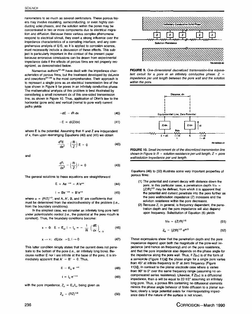
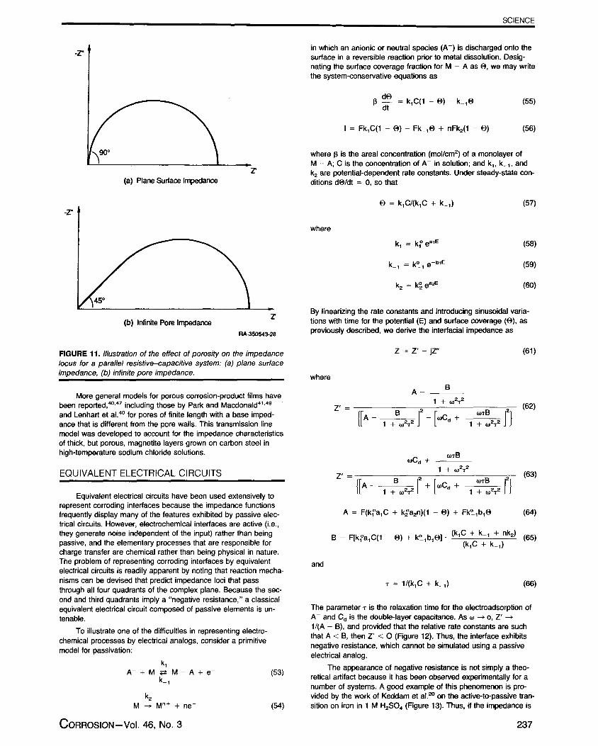
Numerous authors37-49 have dealt with the impedance char-acteristics of porous films, but the treatment developed by deLevieand coworkers37-39 is the most comprehensive. Their approach isto represent a single pore as an electrical transmission line of thetype shown in Figure 9 for pores in an infinitely conductive phase.The mathematica) analysis of this problem is best illustrated byconsidering a small increment dx of this one-sided transmissionline, as shown in Figure 10. Thus, application of Ohm's law to thehorizontal (pore axis) and vertical (nomal to pore wall) currentpaths yields

-dE = IR dx (40)

-E = di(Z/dx) (41)

where E is the potential. Assuming that R and Z are independentof x, then upon rearranging Equations (40) and (41) we obtain

2

d'E -(Z)E=0 (42)

and

- - (- )'=° (43)

The general solutions to these equations are straightforward

E = Ae-"x + A'e°x (44)

i = Be-«x + B'ex (45)

where a = (R/Z)'^, and A, A', B, and B' are coefficients thatmust be determined from the electrochemistry of the problem (i.e.,from the boundary conditions).

In the simplest case, we consider an infinitely long pore heldunder potentiostatic control (i.e., the potential at the pore mouth isconstant). Thus, the boundary conditions become:

x = 0: E = E0,i=1o= _ 1 (dE)

(46)R l dx o

x->x: dE/dx-0,i-0

(47)

This latter condition simply states that the current does not pene-trate to the bottom of the pore (i.e., an infinitely long bore). Be-cause neither E nor i are infinite at the base of the pore, it is im-mediately apparent that A' = B' = 0. Thus,

E = Eo e- °x (48)

i = 10 e'°° (49)

with the pore impedance, Zp = Eo/lo , being given as

Zp = (RZ)' 12 (50)

IMinitely Conductive Solid Phase

z z z z z

Solution Resistance

FIGURE 9. One-dimensional discretized transmission-line equiva-lent circuit for a pore in an infinitely conductive phase: Z =impedance per unit length between the pore walt and the solutionwithin the pore.

Distance, dx

1 I

Equipotential Line, Zero Potential

Z/dx Z/dx îdi

Rdx

E + dE —► E —►i i-di

RAa20522.41

FIGURE 10. Smalt increment dx of the discretized transmission lineshown in Figure 9: R = solution resistance per unit length, Z = porewall/solution impedance per unit length.

Equations (48) to (50) illustrate some very important properties ofporous films:

(1) The potential and current decay with distance down thepore. In this particular case, a penetration depth 1/« =(IZI/R)'^ may be defined, from which it is apparent thatthe potential and current penetrate into the pore further asthe pore walt/solution impedance (Z) increases and thesolution resistance within the pore decreases.

(2) Because Z, in general, is frequency dependent, the pene-tration depth and the pore impedance wilt also dependupon frequency. Substitution of Equation (6) yields

1/« _ (IZI/R) 12 (51)

Zp = (ZIR)1i2 e 2 (52)

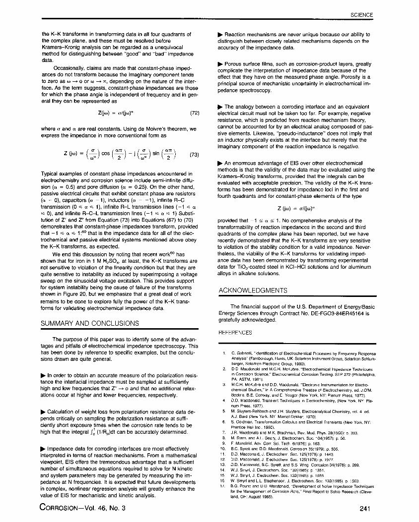
These expressions show that the penetration depth and the poreimpedance depend upon both the magnitude of the pore-walt im-pedance (and hence on frequency) and on the pore resistance,and that the pore impedance also depends on the phase angle forthe impedance along the pore wall. Thus, if Z(W) is of the form ofa semicircle (Figure 11 [a]) the phase angle for a single pore variesfrom 450 at infinite frequency to 0° at zero frequency (Figure11 [b]), in contrast to the planar electrode case where d, variesfrom 90° to 0° over the same frequency range (assuming no un-compensated series resistance). Likewise, if Z(w) is a diffusionalimpedance, then 4) will be equal to 22-1/2° assuming an infinitelylong pore. Thus, a porous film containing no diffusional elementsmimics the phase angle behavior of finite diffusion to a planar sur-face; clearly a large potential exists for misinterpretating imped-ance data if the nature of the surface is not known.

236 CORROSION—March 1990

SCIENCE

Z(a) Plane Surface lmpedance

Z(b) Infinite Pore Impedance

RA-350543-28

FIGURE 11. lllustration of the effect of porosity on the impedancelocus for a parallel resistive-capacitive system: (a) plane surfaceimpedance, (b) infinite pore impedance.

More general models for porous corrosion-product films havebeen reported, 40 •47 including those by Park and Macdonald41 .4°

and Lenhart et al. 40 for pores of finite length with a base imped-ance that is different from the pore walls. This transmission linemodel was developed to account for the impedance characteristicsof thick, but porous, magnetite layers grown on carbon steel inhigh-temperature sodium chloride solutions.

EQUIVALENT ELECTRICAL CIRCUITS

Equivalent electrical circuits have been used extensively torepresent corroding interfaces because the impedance functionsfrequently display many of the features exhibited by passive elec-trical circuits. However, electrochemical interfaces are active (i.e.,they generate noise independent of the input) rather than beingpassive, and the elementary processes that are responsible forcharge transfer are chemical rather than being physical in nature.The problem of representing corroding interfaces by equivalentelectrical circuits is readily apparent by noting that reaction mecha-nisms can be devised that predict impedance loci that passthrough all four quadrants of the complex plane. Because the sec-ond and third quadrants imply a "negative resistance," a classicalequivalent electrical circuit composed of passive elements is un-tenable.

To illustrate one of the difficulties in representing electro-chemical processes by electrical analogs, consider a primitivemodel for passivation:

k,A- +M F M-A+e -(53)

k2M -^ M" + + ne- (54)

in which an anionic or neutral species (A - ) is discharged onto thesurface in a reversible reaction prior to metal dissolution. Desig-nating the surface coverage fraction for M - A as 0, we may writethe system-conservative equations as

13 tl© = k,C(1 - 0) - k_,O (55)

1 = Fk,C(1 - 0) - Fk_,O + nFk2(1 - 0) (56)

where 13 is the area) concentration (mol/cm2) of a monolayer ofM - A; C is the concentration of A- in solution; and k,, k_,, andk2 are potential-dependent rate constants. Under steady-state con-ditions dO/dt = 0, so that

0 = k,C/(k,C + k_,) (57)

where

k, = k; e

k_, = k°, e-b' E (59)

k2 = k2 ea2E (60)

By linearizing the rate constants and introducing sinusoidal varia-tions with time for the potential (E) and surface coverage (0), aspreviously described, we derive the interfacial impedance as

Z = Z' - jZ" (61)

where

A- BZ w2T2

(62)

{[A_ 1 +B 2T2 ,2 — [

_Cd + 1 + W2T2 ]2I

1 +

wCd + wTB

1 + w2T2Z = (63)

lLA — 1 B W2^ J2 + [

.Cd + 1 + (2T2 J2}

A = F(k,a,C + k2a2n)(1 - O) + Fk° 1 b 1 0 (64)

B = F[k, a,C(1 - 0) + k° 1 b,0] • (k,C + k_, + nk2)

(65)(k,C + k_,)

and

T = 1/(k,C + k_,)

(66)

The parameter T is the relaxation time for the electroadsorption ofA- and Cd is the double-layer capacitance. As w -* o, Z' -^1/(A - B), and provided that the relative rate constants are suchthat A < B, then Z' < 0 (Figure 12). Thus, the interface exhibitsnegative resistance, which cannot be simulated using a passiveelectrical analog.

The appearance of negative resistance is not simply a theo-retical artifact because it has been observed experimentally for anumber of systems. A good example of this phenomenon is pro-vided by the work of Keddam et al. 2° on the active-to-passive tran-sition on iron in 1 M H2SO4 (Figure 13). Thus, if the impedance is

-Z"

-r

CORROSION—Vol. 46, No. 3 237

SCIENCE

b0 (Am) ------- 1.0

.3 0.9

02 e( Q i 0.7

0.6

-5 1 0.5

300 0 0.2 0.4 0.6

E (vols)

20010-3

10010.2

106 /,tod 103 \100 J0.110 1

-300 -200 -100 0 100 200 300

r (n.ern2)RA.350513-28

FIGURE 12. Impedance locus predicted by primitive passivationmodel at E = 0 V. Parameters: n = 2, [—Al = 10-6 mol/cm3, Cd =20 µF/cmz, k°, = 10 -70 mol/cm2•s, k' = 10 -8 mol/cm2 •s, a, = 10V- ', b, = 8 V- ', a2 = 5V, 13 = 10-8 mol/cme. Numbers on locusare frequencies (Hz). lnsert: Log 1 (current) and 0 (surface coverage)vs voltage.

200•00

51225

E 400

< 150

200n

0 '' 0-0.1 0 0.1 02 -200 0 200

E—VrsSSE z'—nam=

g 12k ca

i Ok

0 44 Sk 12t 0 8¼ 12. 18k

z . —nC 2

A- E . -0.050 V vs Mg!M0SO e . K2SOa hert

B: E = 0.150V w MdH12SO4 . K 25O4 1w)

C: E .0350V ,n Nl/H12SOa . K2504 1x11

RA-32052232

FIGURE 13. Steady-state polarization curve and complex planeimpedance dia grams at selected potentials through the active-to-passive transition for iron in 1 M H2SO4 as reported by Keddam,Lizee, Pallotta, and Takenouti:2O (A) E = —0.050 V vs Hg/Hg2SO4 ,K2SO4 (set.); (B) E = —0.150 V vs Hg/Hg2SO4, K2SO4 (sat.); (C) E= —0.250 V vs Hg/Hg 2SO4, K2SO4 (sat.). The arrows indicate thedirection of decreasing frequency.

measured at point A, which lies within the active-to-passive transi-tion, the impedance locus intersects the real axis at w --> o at anegative value, although at high frequencies much of the imped-ance locus lies within the first quadrant. At higher potentials, thecurrent becomes independent of potential and the low-frequencyresponse is adequately simulated as a capacitor (at least for pointB). However, at higher frequencies, a loop reminiscent of thatfound for aluminum in 4 M KOH appears in the impedance locus(Figures 7 and 8). This loop does not appear to be accountable forin terms of an equivalent electrical circuit.

White some interfacial corrosion processes undoubtedly maybe modeled as equivalent electrical analogs, in that the analogsmay reproduce the frequency dispersions of the impedances, theexamples given above clearly show that the analogy between acharge-transfer interface and a passive electrical circuit must notbe taken too far. The problem arises from the physical interpreta-tion of the passive elements contained in the equivalent circuit;thus fourth quadrant impedances do not imply "inductance" in thesense of a passive inductor, but rather that the imaginary compo-nent of the reaction impedance is negative. Clearly, in the first in-stance, impedance data should be interpreted in terms of reactionmechanisms because that is the principal source of reactance atlow frequencies (i.e., at frequencies lower than double-layer charg-ing).

KRAMERS—KRONIG TRANSFORMS

At this point it is fitting to ask the question: "How do 1 knowthat my impedance data are correct?" This question is particularlypertinent in view of the rapid expansion in the use of impedancespectroscopy over the past decade, and because more complexelectrochemical and corroding systems are being probed. Thesegive rise to a variety of impedance spectra in the complex plane,including those that exhibit pseudo-inductance and intersectingloops in the Nyquist domain. By merely inspecting the experimen-tal data, it is not possible to ascertain whether or not the data arevalid or have been distorted by some experimental artifact. How-ever, this problem can be addressed by using the Kramers—Kronig(K—K) transforms',55' as recently described by Macdonald andUrquidi-Macdonald50 and Urquidi-Macdonald, Real, andMacdonald.s'

The derivation of the Kramers—Kronig transforms 7 -50,51 •1 isbased on the fulfillment of three general conditions of the system:

Causality — The response of the system is due only to theperturbation applied and does not contain significant componentsfrom spurious sources.

Linearity — The perturbation/response of the system is de-scribed by a set of linear differential laws. Practically, this condi-tion requires that the impedance be independent of the magnitudeof the perturbation.

Stability — The system must be stable in the sense that itreturns to its original state after the perturbation is removed.

If the above conditions are satisfied, together with the trivialcondition that the integrals can be evaluated, the K—K transformsare purely a mathematica) result and do not reflect any other phys-ical property or condition of the system. These transforms havebeen used extensively in the analysis of electrical circuits(Bode54), but only rarely in the case of electrochemicalsystems. s2-57

The Kramers—Kronig transforms may be stated as follows:

Z'(w) — Z'Í^) _ (2 ` ^xx Z"(x) — wZ"(w)

dx (67)71'J O x — w2

Z (w) — Z (o) — 2w ' [( )Z„(x) Z"(w)] 1 dx (68)(-;-) a x x2 — w2

238 CORROSION—March 1990

JA-7759-7

SCIENC E

Z „(w) — —( 2w ) r^ Z ' (x) — wZ'(w) dx (69)

r Jo X2 — w2

4(w) _ 2w ^^ n x)h dx (70)

7r o x — w

where 4(w) is the phase angle, Z' and Z” are the real and imagi-nary components of the impedance, respectively, and w and x arefrequencies. Therefore, according to Equation (8), the polarizationresistance simply becomes

R = (2) i: [ z

,(X) ] dx - (2) i:m: [ Z(x) 1 dx (71)P

7r o X 7Txmin x

100

50N

0

0.58

t ti

tl10 K 1_ 1 1.0.01

50 100 150 200

Z' (2)

where xma„ and xm;,, are the maximum and minimum frequenciesselected such that the error introduced by evaluating the integralover a finite bandwidth, rather than over an infinite bandwidth, isnegligible.

To illustrate the application of the K-K transforms for validat-ing polarization-resistance measurements in particular, and for ver-ifying impedance data in general, we consider the case of Ti02-coated carbon steel corroding in HCI/KCI solution (pH = 2) at25°C. 58 The complex plane diagram for this case is shown inFigure 14, illustrating that at high frequencies the locus of points isIinear with a slope of =11/4, but that at low frequencies the locuscurls over to intersect the real axis. Application of Equation (71)predicts a polarization resistance of 158.2 ft compared with avalue of 157.1 fl calculated from the differente between the high-and low-frequency intercepts on the real axis. sx

By using the full set of transforms, as expressed by Equa-tions (67) to (70), it is possible to transform the real componentinto the imaginary component and vice versa. 51 .17 These trans-forms therefore represent powerful criteria for assessing the valid-ity of experimental impedance data. The application of these trans-forms to the case of Ti02-coated carbon steel is shown in Figures15 and 16. The accuracy of the transforms was assessed by firstanalyzing synthetic impedance data calculated from an equivalentelectrical circuit. An average error between the "experimental" and"transformed" data of less than 1% was obtained. In this case, theresidual error may be attributed to the algorithm used for evaluat-ing the integrals in Equations (67) and (69). A similar level of pre-cision was observed on transforming the extensive data set forTi02-coated carbon steel in HCI/KCI. 56 •57

Not all impedance data are found to transform as well asthose for the equivalent electrical circuit and the Ti0 2-coated car-bon steel system referred to above. For example, Urquidi-Mac-donald, Real, and Macdonald57 •59 have recently applied the K-Ktransforms to the case of an aluminum alloy corroding in 4 M KOHat temperatures between 25 and 60°C, and found that significanterrors occurred in the transforms that could be attributed to interfa-cial instability as reflected in the high corrosion rate.

As an illustration of the above, we show (Figure 17) the Ny-quist diagram for an aluminum alloy (no. 21: 0.1% In - 0.1% TI +0.2% Ga) in 4 M KOH solution at 25°C and under anodic polariza-tion conditions. 59 As shown in Figure 17, the impedance spectrumis dominated at intermediate frequencies by a large pseudo-induc-tive loop. Kramers-Kronig analysis (Figure 18) shows that, despiteconsiderable noise, both the real and imaginary components trans-form correctly, thereby validating the impedance data plotted inFigure 17. This is not the case, however, for the impedance datashown in Figure 19 for the same alloy in the same environmentbut a slightly more positive potential. In this case, the impedancespectrum was also "reproducible," but the data fail to transformcorrectly when subjected to Kramers-Kronig analysis (Figure 20).The cause of failure has been tentatively attributed59 to systemnstability. These studies indicate that the data are probably notaccdptable for mechanistic analyses, even though they were mea-sured under the same experimental conditions as those presentedin Figure 17. However, some questions exist as to the validity of

JA-7572-4

FIGURE 14. Complex plane impedance plot for Ti02-coated carbonsteel in HCIIKCI solution, pH = 2, at 25°C. 56 The parameter isfrequency in Hz.

120 (a)

80

40

0

(b)_ 40cl

N 20

0-1

log w (rad s- ' )JA-7759-6

FIGURE 15. Kramers-Kronig transforms of impedance data forTi02-coated carbon steel in HCIIKCI solution (pH = 2) at 25°C: 57

(a) real impedance component vs log w; (b) comparison of theexperimental imaginary impedance component (----) with Z'(w) data(—) obtained by K-K transformation of the real component.

40 (a)iÁ

20

0

120(b)

80

N40

0-1

Iogw (rad s')

FIGURE 16. Kramers-Kronig transforms of impedance data forTi02-coated carbon steel in HCI/KCI solution (pH = 2) at 25°C: 57

(a) imaginary impedance component vs log w; (b) comparison of theexperimental real impedance component (----) with Z'(w) dataobtained by K-K transformation of the imaginary component.

CORROSION—Vol. 46, No. 3 239

SCIENCE

w

5

É 0U

-5N

-40 -30 -20 0 10 20 30 40 -10 `✓

Z' (S2 • cm2)-15

5 0 5 10 15 20 25

JA-7572-44B Z' (S2 • cm)JA-7572-46A

FIGURE 17. Nyquist diagram for alloy no. 21 in 4 M KOH at 25°C andat E = -1430 mV vs Hg/HgO. 62 (The applied potential is corrected

FIGURE 19. Nyquist diagram for alloy 21 in 4 M KOH at 25°C andfor IR drop.)at E = -1404 mV vs Hg/Hg0. 57 (The applied potential value is

corrected for IR drop.)

20

10

NE 0U

c -10

-20

la!

^Experimental Values

Theoretical Values from KK

80

40

E00

N0

-40

0 1 2 3 4 5

LOG w (rad/s)

1

Experimental Values

/ Theoretical Values from KK

80

40

Eó 0

-40

-80

(a)

-1 0 1 2 3 4 5

LOG w (rad/s)

80

40

Eó 0

N

-40

_80

1 1

Theoretical Values from KK (b)

i/"Experimental Values40

E0 0

N

-40

-Rn

:ical Values from KK

Experimental Values

(b)

-1 0 1 2 3 4 5 -2 -1 0 1 2 3 4 5

LOG w (rad/s) LOG w (rad/s)JA-7572-45A

JA-7572-47

FIGURE 18. Comparison of experimental and K-K-transformed FIGURE 20. Comparison of experimental and K-K-transformedimpedance data for alloy 21 in 4 M KOH at 25°C and at E = 1437 impedance data for alloy 21 in 4 M KOH at 25°C and at E = -1404mV vs Hg/HgO: (a) real component, (b) imaginary compoent. 59 (The mV vs Hg/HgO: (a) real component, (b) imaginary component. 59

applied potential value is corrected for IR drop.) (The applied potential is corrected for IR drop).

240 CORROSION—March 1990

SCIENCE

the K-K transforms in transforming data in all four quadrants ofthe complex plane, and these must be resolved beforeKramers-Kronig analysis can be regarded as a unequivocalmethod for distinguishing between "good" and "bad" impedancedata.

Occasionally, claims are made that constant-phase imped-ances do not transform because the imaginary component tendsto zero as w -* o or w - -, depending on the nature of the inter-face. As the term suggests, constant-phase impedances are thosefor which the phase angle is independent of frequency and in gen-eral they can be represented as

Z(jw) = Q/(JW)" (72)

where or and a are real constants. Using de Moivre's theorem, weexpress the impedance in more conventional form as

-Z (jw)- \ w" ) cos ( 2 / j \ W / sin ( 2 / (73)

Typical examples of constant phase impedances encountered inelectrochemistry and corrosion science include semi-infinite diffu-sion (a = 0.5) and pore diffusion (a = 0.25). On the other hand,passive electrical circuits that exhibit constant phase are resistors(a = 0), capacitors (a =1), inductors (a = - 1), infinite R-Ctransmission (0 -- a -- 1), infinite R-L transmission lines (-1 -- a

0), and infinite R-C-L transmission lines (-1 -- a -- 1) Substi-tution of Z' and Z" from Equation (73) into Equations (67) to (70)demonstrates that constant-phase impedances transform, providedthat -1 __ a _ 1;60 that is the impedance data for all of the elec-trochemical and passive electrical systems mentioned above obeythe K-K transforms, as expected.

We end this discussion by noting that recent work60 hasshown that for iron in 1 M H 2SO4 , at least, the K-K transforms arenot sensitive to violation of the linearity condition but that they arequite sensitive to instability as induced by superimposing a voltagesweep on the sinusoidal voltage excitation. This provides supportfor system instability being the cause of failure of the transformsshown in Figure 20, but we emphasize that a great deal of workremains to be clone to explore fully the power of the K-K trans-forms for validating electrochemical impedance data.

SUMMARY AND CONCLUSIONS

The purpose of this paper was to identify some of the advan-tages and pitfalls of electrochemical impedance spectroscopy. Thishas been done by reference to specific examples, but the conclu-sions drawn are quite general.

In order to obtain an accurate measure of the polarization resis-tance the interfacial impedance must be sampled at sufficientlyhigh and low frequencies that Z" - o and that no additional relax-ations occur at higher and lower frequencies, respectively.

Calculation of weight loss from polarization resistance data de-pends critically on sampling the polarization resistance at suffi-ciently short exposure times when the corrosion rate tends to behigh that the integral fó (1/Rp)dt can be accurately determined.

Impedance data for corroding interfaces are most effectivelyinterpreted in terms of reaction mechanisms. From a mathematicalviewpoint, EIS offers the tremeondous advantage that a sufficientnumber of simultaneous equations required to solve for N kineticand system parameters may be generated by measuring the im-pedance at N frequencies. It is expected that future developmentsin complex, nonlinear regression analysis will greatly enhance thevalue of EIS for mechanistic and kinetic analysis.

Reaction mechanisms are never unique because our ability todistinguish between closely related mechanisms depends on theaccuracy of the impedance data.

Porous surface films, such as corrosion-product layers, greatlycomplicate the interpretation of impedance data because of theeffect that they have on the measured phase angle. Porosity is aprincipal source of mechanistic uncertainty in electrochemical im-pedance spectroscopy.

The analogy between a corroding interface and an equivalentelectrical circuit must not be taken too far. For example, negativeresistance, which is predicted from reaction mechanism theory,cannot be accounted for by an electrical analog composed of pas-sive elements. Likewise, "pseudo-inductance" does not imply thatan inductor physically exists at the interface but merely that theimaginary component of the reaction impedance is negative.

An enormous advantage of EIS over other electrochemicalmethods is that the validity of the data may be evaluated using theKramers-Kronig transforms, provided that the integrals can beevaluated with acceptable precision. The validity of the K-K trans-forms has been demonstrated for impedance loci in the first andfourth quadrants and for constant-phase elements of the type

Z (jw) = cr/(jw)"

provided that -1 <_ a <_ 1. No comprehensive analysis of thetransformability of reaction impedances in the second and thirdquadrants of the complex plane has been reported, but we haverecently demonstrated that the K-K transforms are very sensitiveto violation of the stability condition for a valid impedance. Never-theless, the viability of the K-K transforms for validating imped-ance data has been demonstrated by transforming experimentaldata for T'02-coated steel in KCI-HCI solutions and for aluminiumalloys in alkaline solutions.

ACKNOWLEDGMENTS

The financial support of the U.S. Department of Energy/BasicEnergy Sciences through Contract No. DE-FGO3-84ER45164 isgratefully acknowledged.

REFERENCES

1 C. Gabrielli, "Identification of Electrochemical Processes by Frequency ResponseAnalysis" (Farnborough, Hants, UK: Solartron Instrument Group, Solartron Schlum-berger, Solartron Electronic Group, 1980).

2. D.D. Macdonald and M.C.H. McKubre, "Electrochemical Impedance Techniquesin Corrosion Science," Electrochemical Corrosion Testing, STP 272 (Philadelphia,PA: ASTM, 1981).

3. M.C.H. McKubre and D.D. Macdonald, "Electronic Instrumentation for Electro-chemical Studies," in A Comprehensive Treatise of Electrochemistry, ed. J.O'M.Bockris, B.E. Conway, and E. Yeager (New York, NY: Plenum Press, 1977).

4. D.D. Macdonald, Transient Techniques in Electrochemistry, (New York, NY: Ple-num Press, 1977).

5. M. Sluyters-Rehbach and J.H. Sluyters, Electroanalytical Chemistry, vol. 4, ed.A.J. Bard (New York, NY: Marcel Dekker, 1970).

6. S. Goldman, Transformation Calculus and Electrical Transients (New York, NY:Prentice Hall Inc., 1950).

7. J.R. Macdonald and M.K. Brachman, Rev. Mod. Phys. 28(1956): p. 393.8. M. Stern, and A.L. Geary, J. Electrochem. Soc. 104(1957): p. 56.9. F. Mansfeld, Adv. Corr. Sci. Tech. 6(1976): p. 163.

10. B.C. Syrett and D.D. Macdonald, Corrosion 35(1979): p. 505.11. D.D. Macdonald, J. Electrochem. Soc. 125(1978): p. 1443.12. D.D. Macdonald, J. Electrochem. Soc. 125(1978): p. 1977.13. D.D. Macdonald, B.C. Syrett, and S.S. Wing, Corrosion 34(1978): p. 289.14. W.J. Smyrl, J. Electrochem. Soc. 132(1985): p. 1551.15. W.J. Smyrl, J. Electrochem. Soc. 132(1985): p. 1555.16. W. Smyrl and L.L. Stephenson, J. Electrochem. Soc. 132(1985): p. 1563.17. B.G. Pound and D.D. Macdonald, "Development of Noise Impedance Techniques

for the Management of Corrosion Rate," Final Report to Sohio Research (Cleve-land, OH: August 1985).

CORROSION -VoI. 46, No. 3 241

SCIENCE

18. C. Deslouis, 1. Epelboin, M. Keddam, and J.C. Lestrade, J. Electroanal. Chem.,28(1970): p. 57; J.M. Coueignoux and D. Schumann, J. Electroanal. Chem.17(1968): p. 245.

19. 1. Epelboin and R. Wiart, J. Electrochem. Soc. 118(1971): p. 1577.20. M. Keddam, O.R. Matto, and H. Takenouti, J. Electrochem. Soc. 128 (1981): pp.

257, 266; M. Keddam, J-F. Lizee, C. Pallotta, and H. Takenouti, J. Electrochem.Soc. 131(1984): p. 2016.

21. 1. Epelboin, C. Gabrielli, M. Keddam, J-C. Lestrade, and H. Takenouti, J. Electro-chem. Soc. 119(1972): p. 1632.

22. 1. Epelboin, C. Gabrielli, M. Keddam, and H. Takenouti, Electrochim. Acta20(1975): p. 913.

23. R.D. Armstrong and K. Edmondson, Electrochim. Acta 18(1973): p. 937.24. D.D. Macdonald, S. Real, S. Smedley, and M. Urquidi-Macdonald, J.

Electrochem. Soc., in press (1988).25. S. Real, M. Urquidi-Macdonald, and D.D. Macdonald, J. Electrochem. Soc.

135(1988): p.1633.26. M.C.H. McKubre and D.D. Macdonald, J. Electrochem. Soc. 128(1981): p. 524.27. D.D. Macdonald, S. Real, and M. Urquidi-Macdonald, "Development and Evalua-

tion of Anode Alloys tor Aluminum-Air Batteries," Final Report to Eltech Systems/DOE Subcontract 100484-MLM (Chardon, OH: Eltech Systems Corp., 1987).

28. O.R. Brown and J.S. Whitley, Electrochim. Acta 32(1987): p. 545.29. R. Dreef and C.F.W. Norman, J. Electrochem. Soc. 132(1985): p. 2362.30. K.E. Heusler and W. Allgaier, Werkst. Korros. 22(1971): p. 297.31. H. Schweickert, W.J. Lorenz, and H. Friedburg, J. Electrochem. Soc. 127(1980):

p. 1693.32. K.E. Heusler, "Recent Findings on Mechanism of Several Types of Corrosion,"

DECHEMA-Monogr. 198, 93 (1914-1931, Elektrochem. Met.-Gewinnung, Verab.Korros.), pp. 193-211.

33. M. Keddam, O.R. Mattos, and K. Takenouti, J. Electrochem. Soc. 128(1981): pp.257, 266.

34. B.E. Conway, Theory and Principles of Electrode Processes (New York, NY: Ro-land, 1965): E.J. Calvo, in Comprehensive Chemical Kinetics, vol. 26, ElectrodeKinetics: Principles and Methodology (New York, NY: Elsevier, 1986), Chapter 1.

35. J. Ross Macdonald, Impedance Spectroscopy, (New York, NY: John Wiley andSons, 1987).

36. D.D. Macdonald, S. Real, and M. Urquidi-Macdonald, Electrochim. Acta, in press(1990).

37. R. de Levie, Electrochim. Acta 9(1964): p. 1231.38. R. de Levie, Adv. Electrochem. and Electrochem. Eng. 6(1967): p. 329.39. R. de Levie, Electrochim. Acta 11(1965): p. 113.40. S.J. Lenhart, D.D. Macdonald, and B.G. Pound, Proc. l9th IECEC Conference

(1984), p. 875.41. J.R. Park, and D.D. Macdonald, Corros. Sci. 23(1983): p. 295.42. H. Kaiser, K.D. Beccu, and M.A. Gutjahr, Electrochim. Acta 21(1976): p. 539.43. J.P. Candy, P. Fouilloux, C. Gabrielli, M. Keddam, and H. Takenouti, Compt.

Rend. Acad. Sciences Paris 292C(1977): p. 463.44. K. Mund, Siemens Forsch u Entwicke 4(1975): p. 68.

45. J. McHardy, J.M. Baris, and P. Stonehart, J. Appl. Electrochem. 6(1976): p. 371.46. R.D. Armstrong, K. Edmondson, and J.A. Lee, J. Electronal. Chem. 63(1975): p.

287.47. S. Atlung and T. Jacobsen, Electrochim. Acta 21(1976): p. 575.48. J.R. Park, "The Mechanism of the Fast Growth of Magnetite on Carbon Steel Un-

der PWR Crevice Conditions," Ph.D. thesis (Columbus, OH: Ohio State Univer-sity, 1983).

49. D.D. Macdonald and J.R. Park, submitted to Corrosion (1988).50. H. Kramers, Phyzik. Z. 30(1929): p. 521.51. R. de L. Kronig, J. Opt. Soc. Am. 12(1926): p. 547.52. V.A. Tyagai, and G. Ya. Kolbasov, Elektrokhmiya 8(1972): p. 59.53. R.L. Van Meirhaeghe, E.C. Dutoit, F. Cardon, and W.P. Gomes, Electrochim.

Acta. 21(1976): p. 39.54. H.W. Bode, Network Analysis and Feedback Amplifier Design (New York, NY:

Van Nostrand, 1945), Ch. 14.55. M.M. Jaksic and J. Newman, J. Electrochem. Soc. 133(1986): p. 1097.56. D.D. Macdonald and M. Urquidi-Macdonald, J. Electrochem. Soc. 132(1985): p.

2316.57. M. Urquidi-Macdonald. S. Real, and D.D. Macdonald, J. Electrochem. Soc.

133(1986): p. 2018.58. M.C.H. McKubre, unpublished data (1985).59. D.D. Macdonald, S. Real, and M. Urquidi-Macdonald, submitted to J. Mat. Ed.

(1988).60. D.D. Macdonald and M. Urquidi-Macdonald, J. Electrochem. Soc., to be

published (1988).

APPENDIX A

At steady state, V, o = V20 , V30 = V40 , and V50 = V60 (notethat only at the open-circuit potential is V 40 = V50), and since

we obtain the following set of linear simultaneous equations:

UW + V2' +V I ) ar t +V1° DI 2 + V1b AF3 + V;b AI'R

_ (V 1 - V2) AE (A2)

-V2' AI , + (jW + V32 ) DI'2 = ( V2 - V3) AE (A3)

_V2 + (IW + Vá3 ) DI'3 = V3 AE (A4)

(V5b) AF 1 + (V) AI'2 + (Vs) DI' 3 + (jW + V5b + V) AI'H

(VS - V6) AE (A5)

Use of Cramer's ruie therefore yields

o=

()W +V2'+V1 b) V1b V1b

VZ' (jw +V32) 0

1 0 V32 (jW +V)

(V5 ° ) (V5b) (V)

o,

[(Vr V2) Vrb V bV1b

V2 - V3) (jW + V3 2 ) 0 0 AEV3 -V32 ()W+Vq3) 0

(V5 - V6) (V5b) (V5b) UW +V5b +V6")(A7)

A2

(f )+V2' +V1 b) (VE- V2) V1b y1b

- VZi (V2- V3) 0 0AE

0 V3 (1W +V) 0

(V5 b ) (V5- V6) (V56) UW+V5b +Vg")

(A8)

A3

[o+v1

+Vb) V1b (V V) V

V1 (jW +V2) (V2- V3) 0 12DE

V V3 0

V5 b) (V6) (VS- V6) jW+VSb)

(A9)

AH(fW +V2'+V1b )

V (VE- V2)

- Vul (jw + V32) 0 (V2- V3)AE

0 -V32 ()W+Vq3) V3

(V5 b) (V5b) (V5) (V- V6)

(Al 0)(Al)

VI-1

0 AE

0

(jW +VSb+Vs")(A6)

242 CORROSION-March 1990